HIDRA-D: deep-learning model for dense sea level forecasting using sparse altimetry and tide gauge data

This paper introduces HIDRA-D, a novel deep-learning model for basin scale dense (gridded) sea level prediction using sparse satellite altimetry and in situ tide gauge data. Accurate sea level prediction is crucial for coastal risk management, marine operations, and sustainable development. While traditional numerical ocean models are computationally expensive, especially for probabilistic forecasts over many ensemble members, HIDRA-D offers a faster, numerically cheaper, observation-driven alternative. Unlike previous HIDRA models (HIDRA1, HIDRA2 and HIDRA3) that focused on point predictions at tide gauges, HIDRA-D provides dense, two-dimensional, gridded sea level forecasts. The core innovation lies in a new algorithm that effectively leverages sparse and unevenly distributed satellite altimetry data in combination with tide gauge observations, to learn the complex basin-scale dynamics of sea level. HIDRA-D achieves this by integrating a HIDRA3 module for point predictions at tide gauges with a novel Dense decoder module, which generates low-frequency spatial components of the sea level field in the Fourier domain, whose Fourier inverse is an hourly sea level forecast over a 3 d horizon. When comparing 3 d forecasts against satellite absolute dynamic topography (ADT) data in the Adriatic, HIDRA-D achieves a 28.0 % reduction in mean absolute error relative to the NEMO general circulation model. However, while HIDRA-D performs well in open waters, leave-one-out cross-validation at tide gauges indicates limitations in areas with complex bathymetry, such as the Neretva estuary located in a narrow bay, and in regions with sparse satellite ADT data, like the northern Adriatic. Importantly, the model shows robustness to spatially-limited tide gauge coverage, maintaining acceptable performance even when trained using data from distant stations. This suggests its potential for broader applicability in areas with limited in situ observations.

1 Introduction

The ability to accurately predict sea levels has become increasingly vital for proactive planning and mitigation efforts across diverse sectors. Reliable forecasts are crucial for managing coastal risks, optimizing marine operations, and supporting sustainable development in the face of a changing climate. However, predicting sea levels is an inherently complex task. The ocean is a dynamic system influenced by a multitude of interacting factors, including atmospheric pressure, winds, tides, and currents, all operating across a wide range of spatial and temporal scales. Traditional numerical models (Umgiesser et al., 2022; Ferrarin et al., 2020; Madec and the NEMO System Team, 2024) provide an invaluable spatiotemporal insight into the state of the ocean, ranging from density fields to sea levels. This insight however comes at a high numerical price and even then the models often crucially depend on numerically-intensive data assimilation (Bajo et al., 2023) and local bias corrections to remain close to observations. This is especially true in coastal regions characterized by complex bathymetry and rapidly varying hydrodynamic conditions (Umgiesser et al., 2022).

The inherent uncertainties of the model initial conditions, boundary conditions, and even the representation of physical processes themselves necessitate a probabilistic approach when modeling complex geophysical systems (Ferrarin et al., 2023; Bernier and Thompson, 2015; Mel and Lionello, 2014). Instead of a single, deterministic prediction, numerical forecasting systems often employ ensemble modeling, generating multiple simulations with slightly varying initial conditions, forcings, or parameters to capture the envelope of possible sea level outcomes. While this approach improves robustness, it comes at a steep price. The computational cost increases with the number of ensemble members, making high-resolution, real-time forecasting computationally expensive. To overcome this computational barrier, our research has been focused on developing a family of fast deep learning algorithms for sea level predictions, collectively known as HIDRA (Rus et al., 2025d, 2023; Žust et al., 2021). These models are designed to drastically reduce the computational cost of sea level forecasting while maintaining or even exceeding the accuracy of traditional numerical models, a trend increasingly observed in geophysical fluid dynamics domains (Bi et al., 2023; Lam et al., 2023).

However, data-driven approaches face their own challenges, particularly regarding training stability, interpretability, and the preservation of physical conservation laws, which often require careful hybrid modeling strategies (Irrgang et al., 2021). Nevertheless, active research within the machine learning communities on explainable artificial intelligence (XAI) (Samek and Müller, 2019), together with growing efforts to adapt these methods in geoscience (Mamalakis et al., 2022; Chen et al., 2025), offers a promising outlook. We expect that emerging findings from these subfields will increasingly contribute to the interpretability of deep learning methods in geophysics.

The evolution of HIDRA parallels a broader paradigm shift in ocean forecasting, where data-driven models are increasingly outperforming traditional numerical solvers. Recent global initiatives, such as ORCA-DL (Guo et al., 2025), TianHai (Niu et al., 2025), and XiHe (Wang et al., 2024), have successfully employed deep learning to capture 3D ocean dynamics and eddy-resolving features with high physical consistency. At regional scales, architectures like OceanNet (Chattopadhyay et al., 2024) have introduced physics-inspired neural operators for sea-surface height emulation, while MedFormer (Epicoco et al., 2025) and SeaCast (Holmberg et al., 2025) have demonstrated superior forecasting skills specifically within the Mediterranean Sea. Within this rapidly advancing context, our work has focused on the specific challenge of coastal sea level prediction. The initial HIDRA1 model (Žust et al., 2021) established that deep learning could predict sea surface height (SSH) at a single tide gauge with improved accuracy and vastly reduced computational costs compared to operational numerical model NEMO GCM (Ličer et al., 2020). Subsequent iterations, HIDRA2 (Rus et al., 2023) and HIDRA3 (Rus et al., 2025d), addressed early limitations by improving accuracy and utilizing data from neighboring operational stations to handle sensor failures. However, these models remained fundamentally limited to specific sensor locations, lacking the capability to predict sea levels in open waters, a gap that gridded approaches in the wider field have begun to address.

To bridge the gap between coastal point observations and open-ocean dynamics, we introduce HIDRA-D. This model marks a fundamental shift from the sparse prediction capabilities to dense, gridded, two-dimensional sea level forecasts across the entire ocean basin. HIDRA-D incorporates satellite altimetry observations (absolute dynamic topography, or ADT) to learn the spatial patterns of sea level, which presents a unique challenge, as satellite ADT data, while valuable, is extremely sparse and unevenly distributed, both spatially and temporally (see Fig. 1). While advancements exist in interpolating irregularly sampled satellite data, often focusing on variables with greater coverage like sea surface temperature (Barth et al., 2020, 2022) or employing wide-swath altimetry (Fablet et al., 2021; Beauchamp et al., 2023), we specifically leverage along-track sea level altimetry for its extended historical availability.

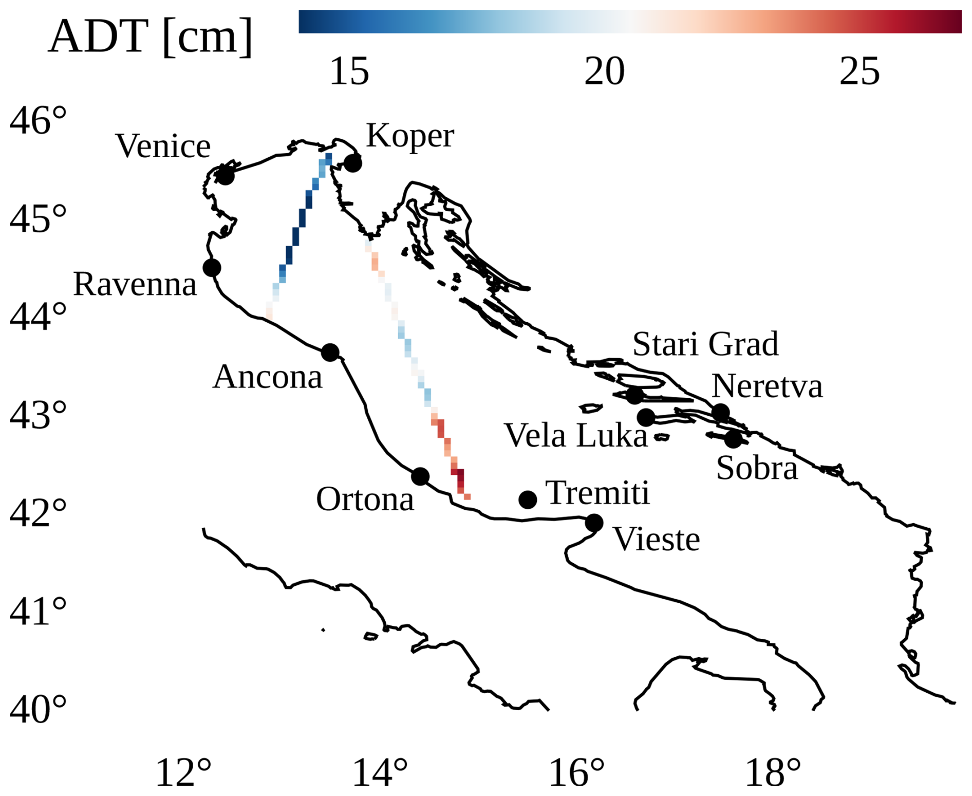
Figure 1 The region of our study, the Adriatic Sea, with 11 tide gauge locations depicted by black dots and along with two satellite absolute dynamic topography (ADT) ground tracks from 6 June 2019 shown.

In the text that follows, ADT (absolute dynamic topography) will be used to denote remote satellite altimetry observations. It is important to note that in this study, our ADT variable is computed as the sum of the sea level anomaly (SLA), mean dynamic topography (MDT), ocean tides, and dynamic atmospheric correction. SSH (sea surface height) will be used to denote local tide gauge observations.

ADT measurements from the satellite altimeter are not calibrated with the SSH measurements at different tide gauges and, furthermore, the tide gauges are often not calibrated between each other, each reporting the sea level values relative to their local vertical datum. In this paper we propose a novel formulation that casts tide gauge and ADT intercalibration as part of the learning problem. Specifically, the model estimates a vertical offset for each tide gauge, effectively aligning all stations to the common satellite-referenced ADT datum. This allows HIDRA-D to function in operational mode, where it generates dense, basin-scale ADT forecasts using only sparse tide gauge observations and atmospheric forcing.

The remainder of this paper is structured as follows. Section 2 details the training and testing datasets, the processing of satellite altimetry, the alignment of heterogeneous data sources, and the NEMO ocean model used for comparison. Section 3 formally defines the prediction problem and provides a detailed description of the HIDRA-D architecture. Section 4 presents an evaluation of HIDRA-D, comparing its dense sea level forecasts against satellite observations and the NEMO general circulation model, as well as analyzing its performance at coastal locations. Finally, Sect. 5 summarizes the main findings and discusses future directions.

2 Data and experimental setup

This section describes the observational data, the numerical models used for comparison, and the preprocessing steps required to align different data sources.

2.1 Training and testing datasets

Our objective is predicting the temporal evolution of sea level in the Adriatic basin on a two-dimensional grid (i.e., dense prediction) with a 3 d horizon at hourly resolution. The horizontal and vertical grid sizes are H=94 and W=115 respectively, spanning a geographical region bounded by latitudes 40.00 to 45.87° N and longitudes 12.20 to 18.85° E. The input to the prediction model consists of past 72 h of available SSH observations from N=11 Adriatic tide gauges together with their respective astronomic tides, as well as the past and future 72 h of gridded geophysical variables obtained by the atmospheric and ocean numerical models.

The training time window spans two intervals: from 2000 to May 2019 and from 2021 to 2022. The testing time window covers the period from June 2019 to the end of 2020. This specific testing interval was selected due to the occurrence of numerous high sea level and coastal flood events in the northern Adriatic and matches the period chosen in our previous work (Rus et al., 2025d).

The following tide gauges along the Adriatic coast are considered in this study for SSH measurements: Koper, Venice, Ancona, Ortona, Vieste, Neretva, Ravenna, Sobra, Stari Grad, Tremiti and Vela Luka (see Fig. 1). To characterize the inter-dependencies within this network, we analyzed the correlation between station records, observing strong clustering between neighboring stations (see Appendix A). Their SSH availability ranges from 15 % to 90 % during years 2000–2022 (Rus et al., 2025d), which has to be accounted for during training and testing, as the model is required to cast predictions also when data from some tide gauges is missing. The raw SSH data, originally recorded at 1 min or 10 min intervals (depending on the station), was filtered using the methods from Rus et al. (2025d) to eliminate three types of sensor errors: (i) sensor freeze, which results in a constant output value for an extended period of time, (ii) extreme outliers, and (iii) extreme jumps in the signals. Subsequently, the measurements were downsampled to hourly resolution. To prevent aliasing and reduce high-frequency noise, we applied a Gaussian smoothing kernel (σ=25 min) using a weighted moving average prior to subsampling. The Gaussian weighted averaging was implemented with dynamic weight normalization to robustly handle missing time-steps in the raw high-frequency series. For each location, the astronomical tides in 1 year intervals were computed using the UTIDE Tidal Analysis package for Python (Codiga, 2011).

Following Rus et al. (2025d), the sea level readings are classified as low if they fall below the 1st percentile and as high if they exceed the 99th percentile of the observed values at the given location (see Rus et al., 2025d, for exact thresholds). During evaluation (Sect. 4.3), several metrics are computed separately for all sea level values and for the aforementioned extreme classes. This enables assessing the model's ability to predict both tails of the sea level distribution: (i) high values, which are crucial for coastal flood warnings, as well as (ii) low values, which may restrict marine traffic in the shallow northern region of the Adriatic basin.

For geophysical variables, we employed ERA5 reanalysis data (Hersbach et al., 2023) for training and ECMWF Ensemble Prediction System (EPS) data (Leutbecher and Palmer, 2007) for evaluation. The reason for using the ERA5 data in training is that our prior research indicated improved performance in the multi-point (i.e., spatially sparse) prediction setup. However, the evaluation is carried out on the ECMWF EPS dataset to faithfully reflect the operational forecasting setup in which reanalysis is unavailable and ensemble forecasts are typically used. The following parameters from ERA5 reanalysis were used: (i) 10 m winds, (ii) mean sea level air pressure, (iii) sea surface temperature (SST), (iv) mean wave direction, (v) mean wave period and significant height of combined wind waves and (vi) the swell data. Following our previous work (Rus et al., 2025d), all input fields were spatially cropped to the Adriatic basin and subsampled to a 9×12 spatial grid.

For operational forecasting and evaluation, an ensemble of n_ens=50 atmospheric members is used. HIDRA-D processes each member separately, generating 50 dense sea level forecasts, which are then averaged to produce the final prediction.

2.2 Satellite altimetry data

To enable supervised training of the network on the entire basin, the along-track sea level anomalies (SLA) from altimeter satellites were acquired from the Copernicus marine service product SEALEVEL_EUR_PHY_L3_MY_008_061. The SLA variables are provided relative to a 20 year mean (1993–2012) with a 1 Hz (∼7 km) sampling resolution. This dataset incorporates data from all available altimeter missions, including Sentinel-6A, Jason-3, Sentinel-3A, Sentinel-3B, Saral/AltiKa, Cryosat-2, Jason-1, Jason-2, Topex/Poseidon, ERS-1, ERS-2, Envisat, Geosat Follow-On, HY-2A, HY-2B, and others. The ADT values used in this study are computed as the sum of the provided variables: SLA_filtered, ocean_tide, mean dynamic topography (MDT) and dynamic atmospheric correction (DAC). Note that ocean_tide (ocean tide correction, or OTC) and DAC are explicitly added back to the anomaly. This effectively reverses the standard altimetry corrections, restoring the high-frequency tidal and atmospheric surge signals that were filtered out, thereby reconstructing the instantaneous total water level observed by tide gauges. This is consistent with how ADT is treated in the CMEMS NEMO model for the purposes of data assimilation (Ali Aydogdu, CMCC, personal communication, 2023) and thus enables comparisons to the NEMO model (Clementi et al., 2021).

For comparisons with hourly measurements from our model or NEMO, the time of a satellite ADT measurement was not rounded to the nearest hour, recognizing that sea level can change rapidly. Instead, hourly time series from our model or NEMO were linearly interpolated to the exact time of each satellite ADT observation. The spatial locations of the satellite ADT measurements were binned into a grid with size 94×115 equal to the spatial output of our model. In cases where multiple satellite ADT measurements fall within the same grid cell, the average of those measurements is taken. For visualization purposes, ADT values are adjusted to have the mean equal to zero. This adjustment is consistent with the model training and evaluation setup, where mean removal is applied as a pre-processing step (see Sect. 2.3).

To validate the satellite altimetry data and assess its accuracy in coastal regions, it is crucial to compare it with independent, in situ measurements. Tide gauges provide reliable SSH observations at specific coastal locations. Therefore, to verify the correlation between satellite ADT and tide gauge SSH measurements, in Fig. 2 we present pairs of ADT and SSH measurements. A satellite ADT measurement is assigned to a tide gauge if it falls within 20 km of its location. If multiple ADT measurements from the same satellite track satisfy this condition, we retain only the closest one. To determine SSH at the time of satellite ADT measurement, we perform linear interpolation between the two nearest SSH observations. To remove bias and focus on the dynamic components, we subtract the mean values of SSH and ADT at each location. Although the measurements come from completely different sources, the visualizations indicate a strong correlation between ADT and SSH, with an average absolute difference of 4.0 cm.

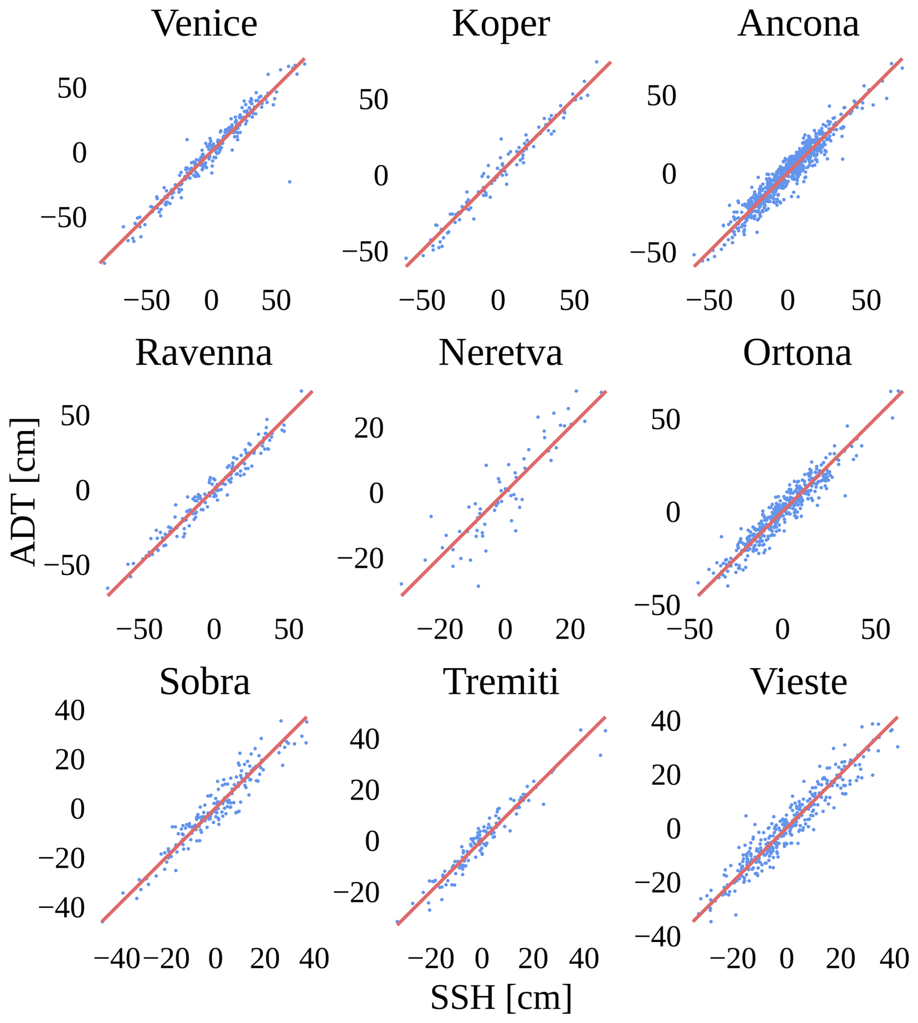
Figure 2 Correlations between satellite (ADT) and tide gauge (SSH) measurements at 9 locations. An ADT measurement is assigned to a tide gauge if it falls within 20 km of its location. The identity line is shown in red. Some degree of discrepancy between ADT and SSH measurements is observed, with an average absolute difference of 4.0 cm.

Despite the availability of ADT data from multiple satellites, its spatial and temporal coverage remains highly uneven. Due to the repetitive nature of satellite orbits, satellite ADT observations are concentrated along specific ground tracks rather than being uniformly distributed. Figure 3 visualizes the spatial distribution of satellite ADT measurements, showing that the majority of observations originate from a limited number of tracks, leaving vast regions with very few satellite ADT measurements.

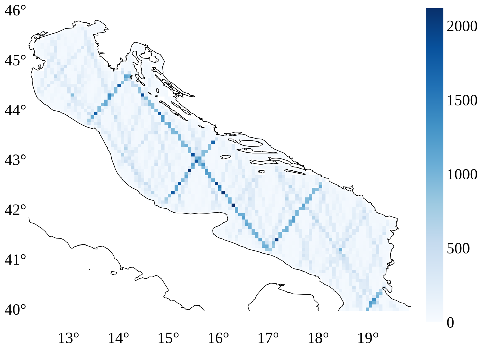
Figure 3 Spatial distribution of count of satellite ADT measurements, where values in the image represent the number of ADT measurements recorded between 2000 and 2020.

Figure 4 illustrates the frequency of tracks between the years 2000 and 2020. Given the high variability of sea level dynamics, satellite ADT data presents an extremely sparse source of ground truth. On average, 2.4 tracks per day are recorded, meaning that in 90 % of hourly intervals, no satellite ADT measurements are available beyond tide gauge measurements. In the remaining 10 % of cases, a single track is present, covering an average distance of 156 km, corresponding to approximately 25 grid points. In our setup, the Adriatic basin covers 3413 grid points, meaning that a single track typically covers less than 1 % of the total number of grid points.

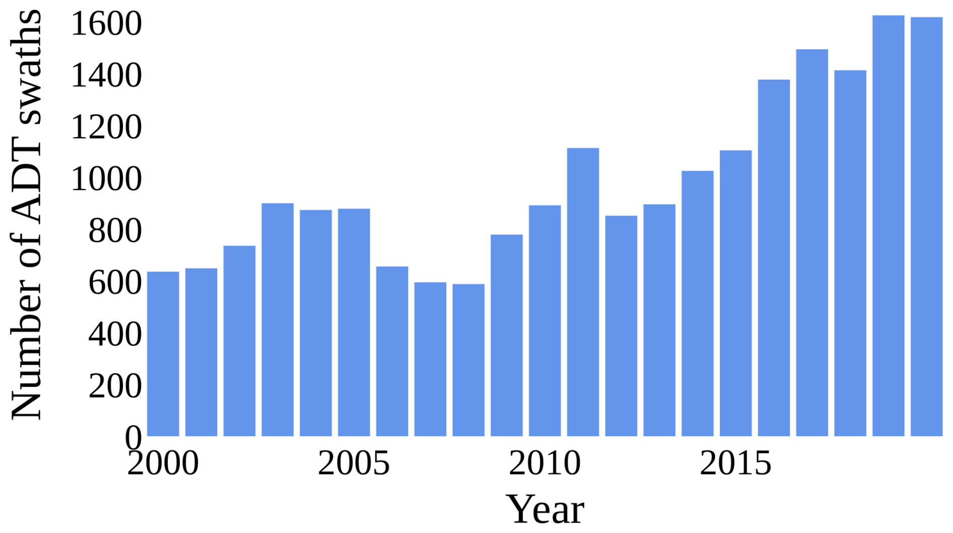
Figure 4 Number of satellite ADT tracks per year from 2000 to 2020. On average, only 2.4 tracks were recorded daily, which highlights the sparsity of the satellite ADT measurements.

2.3 Aligning ADT and tide gauges

A significant challenge in combining satellite altimetry (ADT) and tide gauge data is the lack of calibration between the two sensor types. As defined in Sect. 2.2, ADT represents the level relative to a reference geoid. In contrast, tide gauges measure SSH relative to a local vertical datum, often tied to a local reference ellipsoid. These local reference points are distinct for each tide gauge and their vertical offset from the geoid is generally not readily available. Consequently, without knowing the transformation between tide gauge SSH measurements and satellite ADT measurements, tide gauge data cannot be directly used for supervising the training of a model designed to predict ADT.

To address this discrepancy, we perform a bias correction for each tide gauge i, to convert it into ADT. The following model is used to transform the tide gauge measurements $y_i^{\text{gauge}}$ into ADT ($y_i^{\text{ADT}}$):

$$\begin{array}{}\text{(1)}& y_i^{\text{ADT}}=y_i^{\text{gauge}}+b_i,\end{array}$$

where $y_i^{\text{gauge}}$ is the raw measurement from tide gauge i, and b_i represents the unknown vertical bias for that specific tide gauge relative to the geoid. This displacement primarily represents the offset between the vertical datums, which we assume to be physically constant over the timescales of this study. While vertical land movements can induce slow temporal variations in this offset, these changes are not taken into account here; therefore, we approximate b_i as a constant.

Within our model framework, these unknown bias terms, b_i, are treated as learnable parameters and are estimated concurrently with the main model parameters during the training process. As a pre-processing step, both the satellite ADT dataset and each individual tide gauge time series are independently centered by removing their respective means. Consequently, the training process optimizes the bias parameters b_i to align the centered tide gauge observations with the satellite ADT measurements in their vicinity, effectively connecting the two data sources.

2.4 NEMO model description

The numerical ocean model used in this paper is the Copernicus Marine Environment Monitoring Service (CMEMS) product MEDSEA_ANALYSISFORECAST_PHY_006_013 (Clementi et al., 2021), based on the Nucleus for European Modelling of the Ocean (NEMO) v4.2 (Madec and the NEMO System Team, 2024). The Mediterranean Sea Physical Analysis and Forecasting model (MEDSEA_ANALYSISFORECAST_PHY_006_013) spans a regular grid with a $\mathrm{1}/\mathrm{24}$° (approximately 4 km) horizontal resolution and 141 vertical z*-levels with partial cells to accurately represent the model topography. It employs a staggered Arakawa C-grid with land area masking. Tidal forcing is represented by eight tidal constituents (M2, S2, N2, K2, K1, O1, P1, Q1). The model is forced at its Atlantic lateral boundary by the Global analysis and forecast product (GLOBAL_ANALYSISFORECAST_PHY_001_024) and by a combination of daily climatological fields from a Marmara Sea model and the global analysis product in the Dardanelles Strait. Atmospheric surface forcing is provided by the ECMWF deterministic model. The model was initialized from the World Ocean Atlas (WOA) 2013 V2 winter climatology on 1 January 2015. In situ vertical profiles of temperature and salinity from ARGO, Glider, and XBT, as well as SLA data from multiple satellites (including Jason 2 & 3, Saral-Altika, Cryosat, Sentinel-3A/3B, Sentinel6A, and HY-2A/B) are assimilated via the OceanVar (3DVAR) scheme. The hydrodynamic part of the model is coupled to the wave model WaveWatch-III. We refer the reader to Clementi et al. (2021) for further details.

NEMO computes sea level as a local deviation from the geoid, in theory making it directly comparable to satellite ADT measurements in our setup. However, when analyzing the mean difference between satellite ADT observations and NEMO forecasts (extracted at the satellite ADT measurement locations and linearly interpolated to the corresponding timestamps), we find that, on average, ADT observations are 34.61 cm higher than NEMO forecasts in the training set period. To correct this systematic bias, we apply an offset of 34.61 cm to the NEMO forecasts.

In the analysis of sea level forecasts produced by NEMO, we use the same region defined by HIDRA-D. The region is subsampled from a 141×185 grid to a 94×115 grid to match the resolution of HIDRA-D. This subsampled version is also used when comparing the model to satellite ADT data, ensuring that the metrics are computed on the same set of ADT measurements in the same spatial locations.

3 HIDRA-D: deep learning basin-scale sea level forecasting model

3.1 Formal problem definition of dense sea level prediction

The goal of this study is to predict the temporal evolution of the ADT field, denoted as Y, on a dense two-dimensional grid over the entire Adriatic basin. The target output is a sequence of hourly grid maps over a forecast horizon of T=72 h. The spatial domain is defined by a grid of size H×W (94×115), covering the latitudes 40.00 to 45.87° N and longitudes 12.20 to 18.85° E.

The model approximates the mapping function ℱ such that $\mathbf{Y}=\mathcal{F}({\mathbf{X}}_{\text{SSH}},{\mathbf{X}}_{\text{geo}})$. The inputs consist of sparse SSH (X_SSH), which encompasses the past 72 h of hourly SSH observations from N=11 tide gauges along with their astronomical tide components, and geophysical forcing (X_geo), a tensor containing the past 72 h and forecasted future 72 h of atmospheric and oceanic variables (e.g., wind, pressure, SST) derived from numerical models.

A fundamental challenge in this setting is that the ground truth for the dense output Y (satellite altimetry) is spatially sparse and temporally intermittent. Furthermore, the input tide gauge measurements (y^gauge) and the target satellite data (y^ADT) utilize different vertical datums. Therefore, the problem formulation includes the simultaneous estimation of a set of station-specific bias parameters, $\mathit{\{}{b}_i{\mathit{\}}}_{i=\mathrm{1}}^N$, to align the inputs with the prediction target.

3.2 HIDRA-D model architecture

The primary objective of the HIDRA-D model is to forecast dense sea levels across the basin. A key challenge here is that available inputs are limited to past SSH measurements, which are sparsely located at tide gauge positions, and can be supplemented with geophysical variables such as wind, air pressure, sea surface temperature (SST), and waves. To address the need for a comprehensive understanding of the sea basin's state from these sparse inputs, we leverage our previously developed multipoint SSH prediction model, HIDRA3 (Rus et al., 2025d), described in Sect. 3.2.1. HIDRA3 has proven to be effective in generating a rich latent representation of the sea basin's state, which can subsequently be decoded into accurate SSH predictions at multiple tide gauge locations, including those that were absent from the input. In HIDRA-D, we take this latent representation derived from HIDRA3, along with the aforementioned geophysical features, as the foundation to forecast dense sea level values (see Fig. 5 for architecture). For this purpose, we introduce the Dense decoder module (detailed in Sect. 3.2.2). However, a general challenge in directly forecasting dense sea level fields is the very large output dimensionality, which would typically necessitate a model with a large number of parameters. Furthermore, observed sea level variations are not characterized by an equal distribution of frequencies; rather, low-frequency components account for the majority of sea level fluctuations. Consequently, to make the prediction task more tractable and efficient, we design the Dense decoder module to forecast only these dominant low-frequency components along with their corresponding phases. This forecasting is performed in the 2D Fourier domain for each of the 72-hourly prediction points. The final dense predictions are then efficiently reconstructed by applying the inverse 2D discrete Fourier transform (2D IDFT) to these predicted Fourier coefficients.

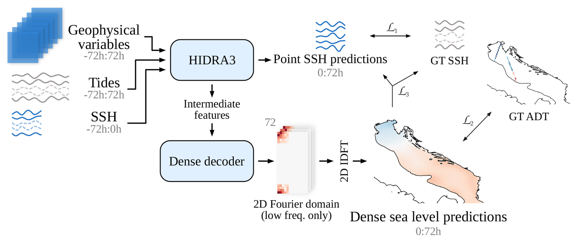
Figure 5 The HIDRA-D architecture. The model is trained end-to-end using a composite loss function: ℒ₁ supervises HIDRA3 point predictions using GT (ground truth) SSH; ℒ₂ supervises dense predictions using available satellite GT ADT; and ℒ₃ ensures consistency between the dense output and tide gauge data (using GT SSH where available, or HIDRA3 point predictions otherwise). Dashed curves in SSH data indicate potential unavailable tide gauge data. The notation a:b indicates hourly data points from the interval (a,b], while the prediction point is at the index 0.

3.2.1 HIDRA3 module

The first step in HIDRA-D’s architecture is the production of SSH point forecasts at all tide gauge locations. For this, we use the HIDRA3 model (Rus et al., 2025d). HIDRA3 takes as input the past 72 h of tide gauge measurements, past and future 72 h of tidal predictions, and past and forecasted 72 h of geophysical variables. Based on these inputs, it generates 72 h SSH forecasts at the tide gauge locations. We selected HIDRA3 due to its strong performance and its ability to handle missing past SSH measurements while consistently providing predictions for all locations. This is crucial for training, as tide gauge data availability varies (see Sect. 2).

While the HIDRA3 module yields predictions for specific tide gauge locations, obtaining dense predictions requires a different approach. Instead of directly using the SSH point predictions, we utilize the intermediate features generated by HIDRA3. Specifically, we extract two key sets of features.

First, we utilize the geophysical feature vector. This vector is produced by HIDRA3’s Geophysical Encoder module, which processes meteorological and oceanographic data fields (wind, air pressure, sea surface temperature, and waves) for the entire forecast region. The input data, covering a 144 h window, is processed through a series of 3D and 1D convolutions to capture both spatial and temporal patterns, ultimately producing a single, comprehensive feature vector s_geo of dimensionality 8192. This vector represents the overall geophysical state of the system.

Second, for each tide gauge i, we employ the per-tide gauge feature vector, denoted as ${\widehat{\mathit{x}}}_i$. These vectors, each with a dimensionality of 1024, are generated within HIDRA3's SSH regression module. Their function is to provide location-specific context for the final forecast. The generation of ${\widehat{\mathit{x}}}_i$ is robust to data availability. If recent SSH measurements for tide gauge i are available, its specific feature vector is computed from that data. However, if measurements are missing, the vector is instead approximated from a joint state vector that aggregates information from all other available tide gauges. This ensures that a unique and informative feature vector ${\widehat{\mathit{x}}}_i$ is available for every tide gauge, which is a key capability we leverage in HIDRA-D.

3.2.2 Dense decoder module

The architecture of the Dense decoder module is shown in Fig. 6. The module processes geophysical features s_geo of size 8192 and N station-specific feature vectors ${\widehat{\mathit{x}}}_i$ of size 1024 each (see Fig. 6). Here, N represents the number of tide gauge stations. These features are concatenated into a single vector of size $\mathrm{8192}+N\times \mathrm{1024}$, with a dimension of 19 456 in our configuration. To reduce dimensionality and computational load, a dense (fully connected) layer with 8192 output channels is applied.

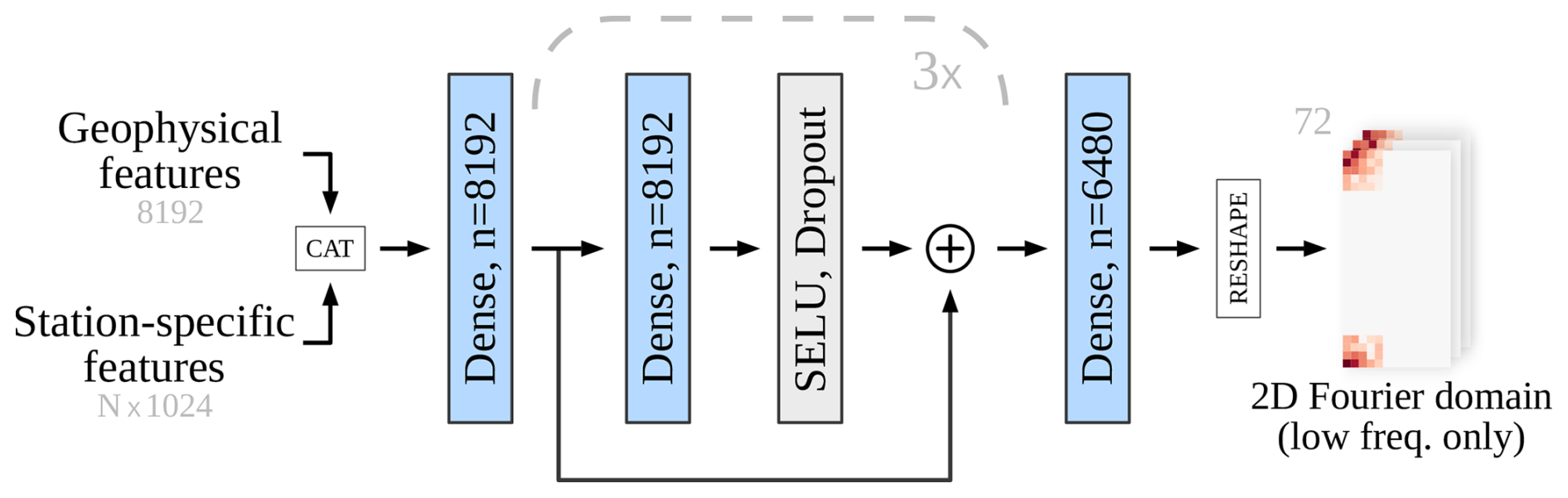
Figure 6 Structure of the Dense decoder module. Geophysical features and station-specific feature vectors are concatenated and processed through multiple dense layers that include SELU activation, dropout, and residual connections. The final output vector is reorganized (reshaped) into a tensor format, where the predicted values are assigned as coefficients to the low-frequency components in the 2D discrete Fourier domain (ready for the Inverse DFT shown in Fig. 5).

The output is passed through three additional dense layers, each with 8192 output channels. These layers incorporate Scaled exponential linear unit (SELU, Klambauer et al., 2017) activation, dropout, and residual connections, as depicted in Fig. 6. Residual connections help preserve input features by enabling the network to learn additive, nonlinearly transformed features. SELU is chosen over Rectified linear unit (ReLU, Nair and Hinton, 2010) for its superior gradient propagation characteristics, while dropout is employed as a standard regularization technique to prevent overfitting.

As discussed in Sect. 2.2, satellite ADT data is extremely sparse and concentrated along specific ground tracks (Fig. 3). This sparsity can negatively impact model performance by potentially introducing unrealistically sharp sea level gradients at spatial scales considerably smaller than the local barotropic Rossby radius. Recognizing that large-scale forcings drive low-frequency components that account for a significant portion of sea level variability, our modeling approach focuses exclusively on these components. The threshold for this frequency selection is determined by the barotropic Rossby radius. In the shallow northern Adriatic, with depths around 15 m, the Rossby radius is estimated to be approximately 120 km. Based on this, we set a spatial scale threshold of λ_R=150 km, thereby modeling only processes with spatial scales larger than this value. The threshold is ablated in Sect. 4.5.

In the 2D discrete Fourier domain, the complex Fourier transform matrix F has dimensions 94×115. An element F_ab of this matrix corresponds to a pair of spatial frequencies (k_x(a),k_y(b)). These spatial frequencies (inverse spatial scales, $k=\mathrm{2}\mathit{\pi }/\mathit{\lambda }$) are computed as follows:

$$\begin{array}{}\text{(2)}& {\displaystyle }{k}_x\left(a\right)=\left\{\begin{array}{ll}\frac{a}{W}{k}_x^s,& a=\mathrm{0},\mathrm{1},\mathrm{\dots },\lceil \frac{W}{\mathrm{2}}\rceil -\mathrm{1}\\ \frac{a-W}{W}{k}_x^s,& a=\lceil \frac{W}{\mathrm{2}}\rceil ,\mathrm{\dots },W-\mathrm{1}\end{array}\right.\text{(3)}& {\displaystyle }{k}_y\left(b\right)=\left\{\begin{array}{ll}\frac{b}{H}{k}_y^s,& b=\mathrm{0},\mathrm{1},\mathrm{\dots },\lceil \frac{H}{\mathrm{2}}\rceil -\mathrm{1}\\ \frac{b-H}{H}{k}_y^s,& b=\lceil \frac{H}{\mathrm{2}}\rceil ,\mathrm{\dots },H-\mathrm{1}\end{array}\right.\end{array}$$

where W=115 and H=94 are the dimensions (number of grid points) of the spatial grid in the x and y directions, respectively. The terms $k_x^s\approx \mathrm{2}\mathit{\pi }/\mathrm{\Delta }x$ and $k_y^s\approx \mathrm{2}\mathit{\pi }/\mathrm{\Delta }y$ are derived from the grid spacings Δx and Δy. For our domain, these values are $k_x^s\approx \mathrm{1.16}{\mathrm{km}}^{-\mathrm{1}}$ and $k_y^s\approx \mathrm{0.91}{\mathrm{km}}^{-\mathrm{1}}$.

To ensure that only wavelengths λ>λ_R are represented in the output, the model predicts only those Fourier coefficients F_ab for which the corresponding spatial frequencies satisfy $\left|k_x\right(a\left)\right|<\mathrm{2}\mathit{\pi }/{\mathit{\lambda }}_{\mathrm{R}}$ and $\left|k_y\right(b\left)\right|<\mathrm{2}\mathit{\pi }/{\mathit{\lambda }}_{\mathrm{R}}$. Since the model predicts real-valued sea level fields, the Fourier matrix F must be Hermitian. Consequently, it is only necessary to predict approximately half of the Fourier coefficients, as the other half can be computed by transposition and conjugation. Specifically, the output from a Dense decoder populates complex coefficients in F at the lowest spatial frequencies, which in our setup correspond to 5×5 and 4×5 regions in the corners of the matrix F (see Fig. 6). The final dense layer thus outputs a vector of 6480 features (comprising 90 real and imaginary components for each of the 72 forecast lead times). The remaining elements of F, corresponding to higher spatial frequencies, are set to zero. For each of the 72 temporal slices, the matrix F is transformed into a spatial field using an inverse 2D discrete Fourier transform (2D IDFT). The resulting field is then multiplied by a binary land-sea mask of the Adriatic. The final spatial predictions are obtained by concatenating the 72 processed temporal slices, resulting in a grid of size $\mathrm{72}\times H\times W$.

3.3 The loss functions

HIDRA-D is trained end-to-end using a multi-component loss function designed to effectively leverage diverse data sources and provide targeted supervision. While the primary goal is to predict dense sea level maps, relying solely on satellite ADT measurements (denoted as y^ADT) can be insufficient for robustly training the entire network, especially its backbone components. To address this, we incorporate tide gauge SSH measurements (denoted as y^gauge), which, despite their spatial sparsity and missing values, provide valuable supervisory signals.

To foster robust learning of the HIDRA3 module's internal representations, which form the foundation for subsequent dense predictions, a dedicated loss term, ℒ₁, is applied. This loss directly supervises the HIDRA3 module by comparing its SSH predictions ($y_{\mathrm{p}}^{\text{gauge}}$) to local SSH measurements from tide gauges (y^gauge):

$$\begin{array}{}\text{(4)}& {\mathcal{L}}_{\mathrm{1}}=\stackrel{\mathrm{‾}}{(y_{\mathrm{p}}^{\text{gauge}}-y^{\text{gauge}}{)}^{\mathrm{2}}}.\end{array}$$

Here, the overline symbol $\stackrel{\mathrm{‾}}{\left(\mathrm{\dots }\right)}$ denotes the mean taken over all timesteps and all available tide gauge stations. This targeted supervision provides an additional training signal specifically for the HIDRA3 backbone.

The dense 2D sea level predictions $y_{\mathrm{p}}^{\text{grid}}$ are primarily trained using satellite ADT observations. The loss term ℒ₂ measures the mean squared error between the dense ADT predictions ($y_{\mathrm{p}}^{\text{grid}}$) and satellite ADT observations (y^ADT):

$$\begin{array}{}\text{(5)}& {\mathcal{L}}_{\mathrm{2}}=\stackrel{\mathrm{‾}}{(y_{\mathrm{p}}^{\text{grid}}-y^{\text{ADT}}{)}^{\mathrm{2}}}.\end{array}$$

As the dense predictions ($y_{\mathrm{p}}^{\text{grid}}$) have an hourly resolution, we linearly interpolate between two neighboring predictions to match the precise timestamps of the asynchronous ADT measurements from satellites. ℒ₂ extends the learning beyond tide gauge locations, leveraging the broader spatial coverage of satellite data.

To further enhance the training of the Dense decoder and utilize all available data, tide gauge data are also incorporated into its supervision through the loss term ℒ₃. This is particularly beneficial for improving predictions at coastal locations where tide gauges are situated. ℒ₃ measures the mean difference between the dense sea level predictions at tide gauge locations ($y_{\mathrm{p},i}^{\text{grid}}$) and the corresponding tide gauge information. Since tide gauge observations (y^gauge) typically measure local SSH relative to a local datum, they must be transformed to be comparable with the network's predictions. Recall from Sect. 2.3, that this transformation is achieved by adding learned station-specific displacements b_i to the tide gauge SSH observations $y_i^{\text{gauge}}$, effectively converting them into local ADT equivalents.

A challenge with tide gauge data is the frequent unavailability of measurements. To ensure that ℒ₃ is defined over a comprehensive set of points and to provide continuous guidance, missing tide gauge observations $y_i^{\text{gauge}}$ are replaced by the corresponding point SSH predictions ($y_{\mathrm{p},i}^{\text{gauge}}$) from the HIDRA3 module. This is possible because the HIDRA3 module outputs predictions for all tide gauges, even when input measurements for some tide gauges are missing. Consistent with the treatment of $y_i^{\text{gauge}}$, these HIDRA3 predictions are also transformed into the space of ADT by adding the same station-specific displacement b_i. Thus, ℒ₃ is defined as:

$$\begin{array}{}\text{(6)}& {\mathcal{L}}_{\mathrm{3}}=\left\{\begin{array}{ll}\stackrel{\mathrm{‾}}{(y_{\mathrm{p},i}^{\text{grid}}-(y_i^{\text{gauge}}+b_i){)}^{\mathrm{2}}}& \\ & \mathrm{\text{where observation }}{y}_i^{\text{gauge}}\text{ exists},\\ \stackrel{\mathrm{‾}}{(y_{\mathrm{p},i}^{\text{grid}}-(y_{\mathrm{p},i}^{\text{gauge}}+b_i){)}^{\mathrm{2}}}& \\ & \mathrm{\text{where observation }}{y}_i^{\text{gauge}}\text{ does not exist}.\end{array}\right.\end{array}$$

This approach ensures that the Dense decoder module is consistently supervised at all tide gauge locations, leveraging either direct (transformed) observations or transformed HIDRA3 predictions as targets.

The final composite loss function, used for gradient backpropagation during the end-to-end training of the HIDRA-D model, is a weighted sum of these individual loss terms:

$$\begin{array}{}\text{(7)}& \mathcal{L}=\mathit{\alpha }{\mathcal{L}}_{\mathrm{1}}+\mathit{\beta }{\mathcal{L}}_{\mathrm{2}}+\mathit{\gamma }{\mathcal{L}}_{\mathrm{3}}.\end{array}$$

The weights were selected to enforce a hierarchical training structure: α=100, β=1, and γ=1. The significantly higher magnitude of α is a design choice intended to act as a soft constraint, ensuring that the HIDRA3 backbone prioritizes the accuracy of point-based SSH predictions (ℒ₁) above all else. This prevents the optimization of the dense reconstruction losses (ℒ₂ and ℒ₃) from degrading the quality of the underlying backbone representations. Consequently, the backbone learns primarily from the high-fidelity tide gauge data, while the Dense decoder adapts to these representations to satisfy the basin-wide constraints. The weights β and γ are set equally as ℒ₂ and ℒ₃ operate on largely spatially disjoint sets of points (sparse satellite tracks versus fixed tide gauge locations) and therefore do not require competitive weighting.

3.4 Training details

We use the AdamW optimizer (Loshchilov and Hutter, 2017) with initial learning rate of 10⁻⁵ and a weight decay of 0.001. A higher initial learning rate of 10⁻³ is used for training the displacements b_i. We utilize a cosine annealing schedule (Loshchilov and Hutter, 2016) to progressively decay the learning rate from its initial value η to a minimum value of $\mathit{\eta }/\mathrm{100}$ over the course of training. Parameters are initialized using a standard Xavier initialization (Glorot and Bengio, 2010), and parameters of the HIDRA3 module are initialized as described in Rus et al. (2025d). During training, tide gauge failures are simulated by randomly deactivating a subset of tide gauges with a probability of 0.5. The model is trained for 50 epochs with a batch size of 128 data samples. Prior to training, all input data is standardized by subtracting the mean and dividing by the standard deviation. The mean is computed independently for each tide gauge location, while a single standard deviation is determined across all locations. Hyperparameters were tuned using a validation set separate from the test set. To maximize the data available for learning, the final models were trained on the full training dataset (see Sect. 2.1). Each geophysical variable and satellite ADT data undergoes independent standardization. Training requires approximately 12 h on a system equipped with an NVIDIA A100 Tensor Core GPU.

4 Results

4.1 Evaluation of dense sea level predictions over the Adriatic

To assess the accuracy of dense sea level predictions, we compare them against ADT values (i.e., satellite along-track measurements) on the test set, spanning the period from June 2019 to the end of 2020. Table 1 presents the mean absolute error (MAE) and root mean squared error (RMSE) for HIDRA-D and NEMO (Madec and the NEMO System Team, 2024) based on satellite ADT data. The performance of the model against in situ tide gauge measurements requires a specific cross-validation setup to avoid data leakage and is detailed separately in Sect. 4.3 and Table 3. Results indicate that overall HIDRA-D outperforms NEMO, with both MAE and RMSE being significantly lower. Furthermore, HIDRA-D exhibits a very low bias of −0.17 cm. Since we performed a bias correction of NEMO to align it with satellite ADT data (see Sect. 2.4), its bias is effectively zero.

Table 1 Comparison of MAE, RMSE and bias between HIDRA-D and NEMO, based on satellite ADT data over Adriatic basin during the testing period from June 2019 to the end of 2020. Bold values highlight the best performance. The bias for NEMO is zero, as an offset correction was applied to its forecasts. The performance of the model against in situ tide gauge measurements requires a specific leave-one-out setup to avoid data leakage and is detailed separately in Sect. 4.3 and Table 3.

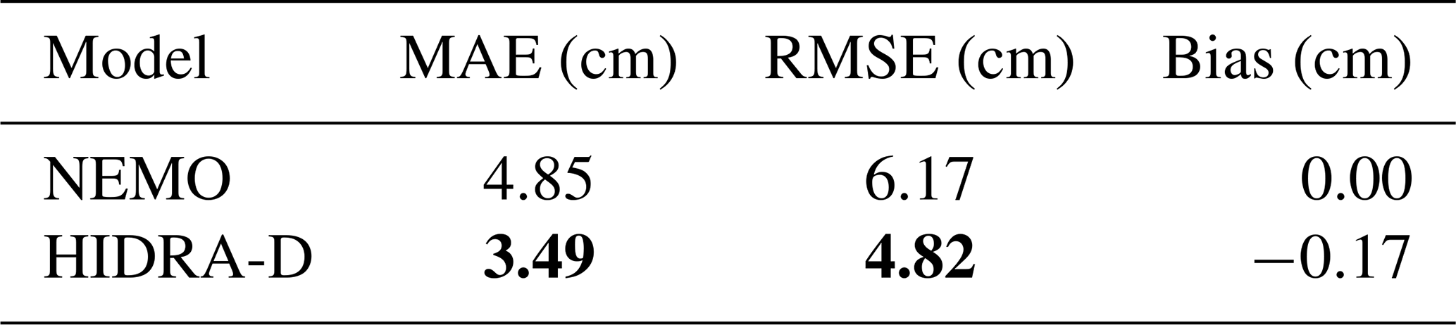
Figure 7 Spatial distribution of the root mean square difference (RMSD) between HIDRA-D and NEMO forecasts for lead times T+1, T+24, T+48, and T+72 h, computed over the test period. Discrepancies are most pronounced in the shallow northern Adriatic and remain stable across all lead times.

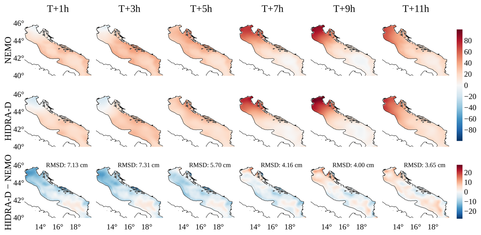
Figure 8 A subset of dense sea level predictions generated by HIDRA-D and NEMO during a storm surge event. The forecasts correspond to T = 14 October 2020, 23:00 UTC, the units are cm. HIDRA-D produces a spatially smoother forecast compared to NEMO. The bottom row illustrates the difference between HIDRA-D and NEMO; note that it has a separate color bar. The root mean squared difference (RMSD) between the two models is indicated in each panel.

To further analyze the spatial and temporal structure of the discrepancies between the models, Fig. 7 illustrates the root mean square difference (RMSD) between HIDRA-D and NEMO across the basin for different forecast lead times. The metric is computed over the entire test period. Visually, the highest RMSD values (reaching approx. 8 cm) are concentrated in the northern Adriatic, likely due to the complex shallow-water dynamics in that region. Comparisons with available satellite ADT measurements (latitude >43.5°) confirm that while both models exhibit higher errors in this area, HIDRA-D performs better with an RMSE of 5.37 cm compared to 6.79 cm for NEMO. In contrast, the central and southern parts of the basin generally exhibit lower differences, mostly ranging between 4 and 6 cm. Notably, both the spatial pattern and the magnitude of the RMSD remain remarkably stable across all lead times, indicating that the divergence between the two models does not grow significantly as the forecast horizon extends from T+1 to T+72 h.

To visually compare the forecasts, we present two examples of dense forecasts generated by HIDRA-D and NEMO, along with the difference between these forecasts. Forecasts under calm atmospheric conditions are presented in Appendix B (Fig. B1), while Fig. 8 depicts the forecasts of dense sea level during a storm surge event. Note that the HIDRA-D predictions are smoother, containing lower spatial frequencies than predictions from NEMO. This result is expected because HIDRA-D does not model processes with spatial scales below the barotropic Rossby radius, λ_R. These smaller-scale processes can be caused by other ocean processes, such as ocean currents, which are not explicitly included in the HIDRA-D model. Despite this difference, both models generally produce forecasts of a comparable magnitude. Due to space limitations only selected parts of the forecasts are presented here, for visualizations of the entire forecast and additional forecasts, we direct the reader to the video supplement of the paper.

Figure 9 compares HIDRA-D and NEMO predictions with along-track satellite ADT observations. Selected dates correspond to the first day of each month from June 2019 to May 2020, with the longest track in the basin chosen for each day. The forecasts were obtained for the same day as the satellite altimetry observations, with model predictions interpolated to match the satellite observation times. The results indicate that while both HIDRA-D and NEMO predictions are both smoother than altimetry observations, HIDRA-D predictions better capture the overall trend reflected in the measurements.

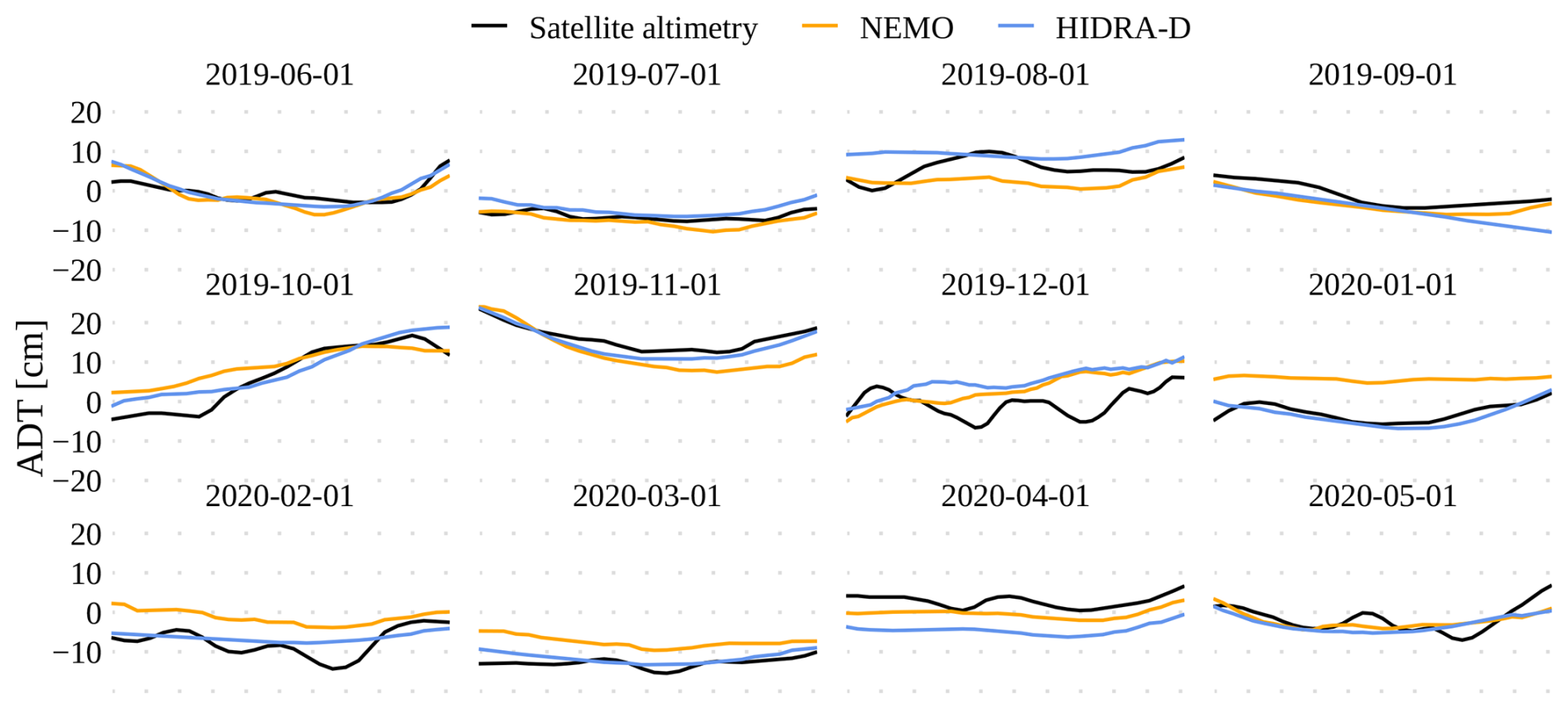
Figure 9 Comparison of along-track satellite ADT measurements with forecasts from HIDRA-D and NEMO. Predictions from both models were interpolated to match the satellite altimetry observation times.

4.2 Learned tide gauge displacements

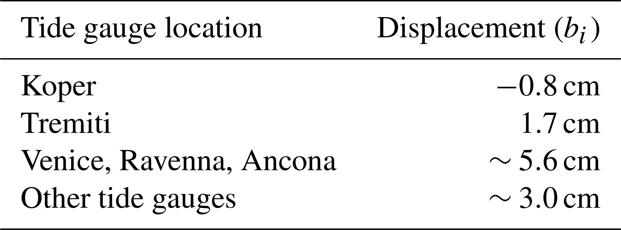
The methodology described in Sect. 2.3 involves learning the vertical displacement, b_i, for each tide gauge i. A positive b_i indicates that, on average, measurements from tide gauge i are lower than satellite ADT measurements in its vicinity. The resulting displacements for the different tide gauge locations are shown in Table 2. The values vary in both sign and magnitude, ranging from −0.8 cm at Koper to +5.6 cm at several Italian locations. This variation underscores the necessity of estimating these displacements individually for each tide gauge, as a single, uniform offset would not suffice to accurately align all tide gauge records to the common ADT reference.

Table 2 Learned vertical displacements (b_i) for each tide gauge. A positive b_i indicates that, on average, measurements from tide gauge i are lower than satellite ADT measurements in its vicinity.

4.3 Performance along the coastal region

This section analyzes the HIDRA-D prediction accuracy at coastal locations to estimate the potential for its practical application in sea level prediction at locations without tide gauges. The evaluation setup involves removing, one at a time, one tide gauge from the total set of N=11 tide gauges, and training a separate model for each excluded tide gauge. Each separate model for each of the eleven tide gauges is therefore trained on 10 remaining tide gauges. When calculating scores or visualizing, we always use the model that was not trained on data from the corresponding tide gauge. When presenting results from such setup, we use the notation HIDRA-D^N, where N=11 refers to the number of models trained and used in the evaluation. Note that since we do not have any information about tide gauges' local vertical datums, bias correction over the test set is applied for each excluded tide gauge and model separately.

We evaluate the models using standard performance measures from Rus et al. (2023): mean absolute error (MAE), root mean squared error (RMSE), accuracy (ACC), bias, recall (Re), precision (Pr), and the F1 score. All metrics presented in Table 3 are averaged over all forecast lead times (from T+1 to T+72 h) and across all tide gauge locations. The table categorizes performance for all sea level values (overall) and separately for low and high sea level values (see Sect. 2 for definitions). Comparing HIDRA-D^N and NEMO, the results indicate that HIDRA-D^N achieves lower errors than NEMO overall, with a particularly significant reduction in error for low SSH values.

Table 3 Performance comparison between HIDRA-D^N and NEMO using tide gauge measurements. The evaluation covers all SSH values (“Overall”), as well as separate metrics for low and high SSH values. The reported scores are averaged over all forecast lead times (T+1 to T+72 h) and over all tide gauge locations. Bold values indicate the best performance in each part of the table.

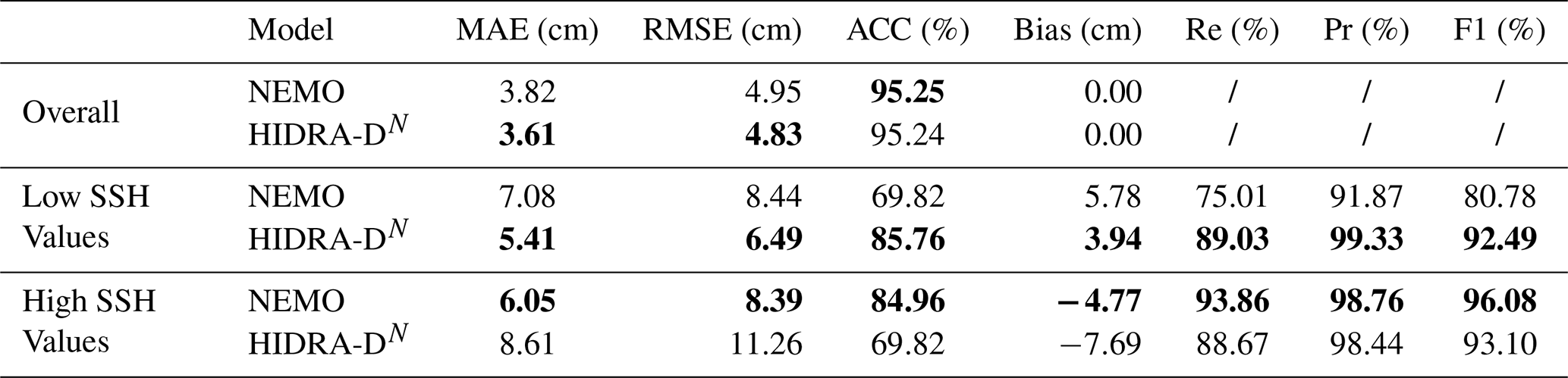
In contrast, for high sea level values, NEMO outperforms HIDRA-D^N. Figure 10 shows RMSE scores for each tide gauge location for further insights. While HIDRA-D^N achieves comparable error levels to NEMO at many locations, it exhibits significantly higher RMSE at Koper, Venice, and Neretva for high sea level values. This discrepancy likely arises from three connected reasons. First, the primary supervision for the dense field comes from satellite ADT data, which is spatiotemporally sparse (Fig. 3); the probability of a satellite track capturing the peak of a transient short-duration storm surge is low, leading to a training set imbalanced against extreme dense events. Second, deep learning models trained with mean squared error objectives tend to produce smoothed outputs to minimize global error, occasionally underestimating sharp peaks (regressing to the mean). Third, extreme values at specific locations are often driven by unresolved local topographic effects in bays and harbors. In the leave-one-out HIDRA-D^N setup, the model must infer these local dynamics without ever seeing training data from that specific coastline geometry, whereas NEMO explicitly solves physical equations using high-resolution bathymetric grids. These findings suggest that HIDRA-D^N is highly effective for open waters and general basin dynamics but faces limitations in resolving localized coastal extremes at locations where it has not been explicitly trained.

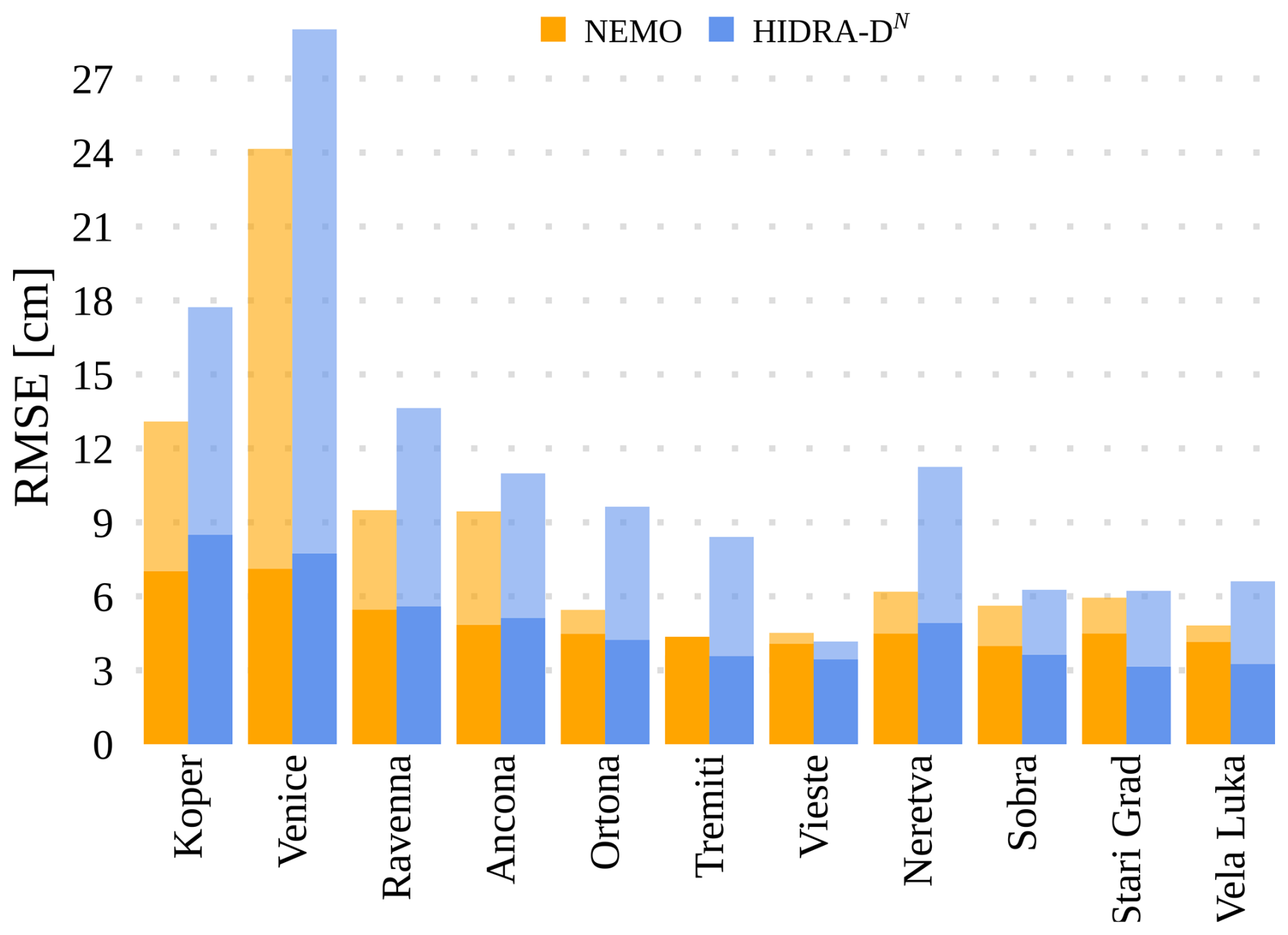
Figure 10 RMSE performance against tide gauge measurements for HIDRA-D^N and NEMO. Solid regions represent the overall RMSE, while semi-transparent regions indicate the RMSE for high SSH values. The models exhibit similar performance overall, while HIDRA-D^N shows larger errors for high SSH values. Note that during training HIDRA-D^N did not see any data from the respective station.

It is important to note, however, that these conclusions apply to an arbitrary point on the coastline where no training data is provided. At training tide gauge locations, HIDRA-D performs marginally worse than HIDRA3. The average RMSE across all stations increases from 3.28 to 3.61 cm. For high sea level values, the RMSE increases from 5.61 to 6.72 cm. For low sea levels, the performance is more similar, with an RMSE of 4.24 cm for HIDRA3 and 4.41 cm for HIDRA-D.

To visually observe the model outputs, we compare the forecasted SSH time series generated by HIDRA-D^N and NEMO against tide gauge measurements. Comparison during a storm surge event is illustrated in Fig. 11, while performance during calm atmospheric conditions is provided in Appendix B (Fig. B2). We can see that both models capture the sea level dynamics well. For additional visualizations, including further forecasts and failure cases, we refer the reader to the video supplement.

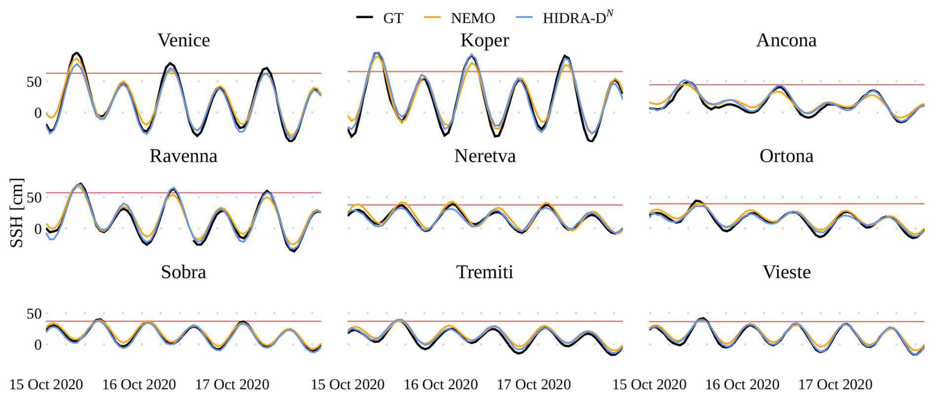
Figure 11 Prediction under storm surge atmospheric conditions. An example of a single forecast from 14 October 2020, 23:00 UTC for HIDRA-D^N and NEMO, compared with tide gauge measurements. The high SSH threshold is marked with a red line. Note that during training HIDRA-D^N did not see any data from the station on each panel.

Dynamic local bias correction

This experiment evaluates the performance improvement in a specific scenario where a tide gauge station, previously unavailable, is newly installed. The introduction of this new tide gauge allows for the application of a dynamic local bias correction at test time, which is not possible before the station is installed. We evaluate the models using tide gauge observations by applying this dynamic local bias correction at each tide gauge rather than a constant one. We apply bias correction to the first 12 h of the forecast, following standard practice when using the NEMO model for tide gauge forecasting (Rus et al., 2023). To distinguish these results from those obtained in previous experiments, we denote the NEMO model with 12 h bias correction as NEMO_b. For comparability, we also apply a 12 h bias correction to HIDRA-D^N, referring to the adjusted model as ${\text{HIDRA-D}}_b^N$.

Table 4 presents the average scores for both models across all tide gauge locations. The results indicate that NEMO_b consistently exhibits lower errors than ${\text{HIDRA-D}}_b^N$. Figure 12 displays the RMSE scores for all tide gauges, showing that ${\text{HIDRA-D}}_b^N$ again produces the highest errors in Koper, Venice, and Neretva, likely for the reasons discussed in Sect. 4.3. These findings suggest that when a newly installed tide gauge is available for bias correction, NEMO_b provides more accurate predictions than ${\text{HIDRA-D}}_b^N$. However, as historical tide gauge data accumulates, training HIDRA-D on this location becomes feasible. In fact, our recent work (Rus et al., 2025d) has shown that jointly trained on several tide gauges, HIDRA3 achieves excellent prediction accuracy at tide gauge locations even with a moderate amount of historical training data.

Table 4 Performance comparison between ${\text{HIDRA-D}}_b^N$ and NEMO_b, both bias-adjusted using the first 12 h of each forecast. The reported scores represent the average across all tide gauge locations. The results indicate that when data from a newly installed tide gauge is available, enabling dynamic bias correction, NEMO_b achieves superior performance compared to ${\text{HIDRA-D}}_b^N$. Bold values indicate the best performance in each part of the table.

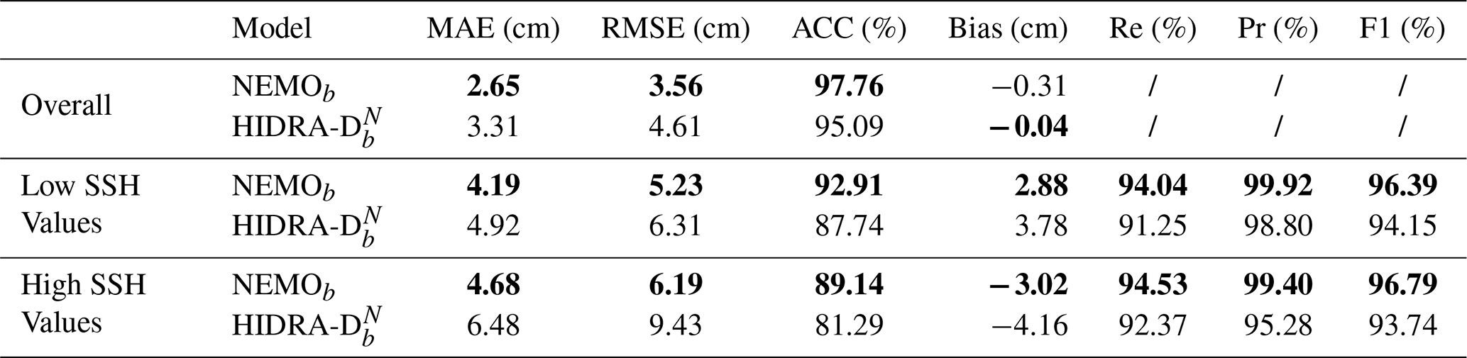
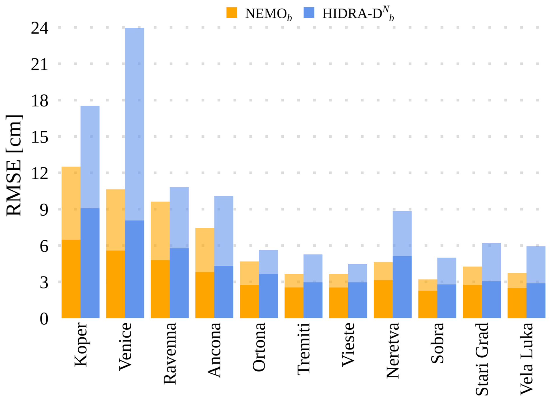
Figure 12 RMSE performance against tide gauge measurements for the ${\text{HIDRA-D}}_b^N$ and NEMO_b models. Solid regions represent the overall RMSE, while semi-transparent regions indicate the RMSE for high SSH values. A bias adjustment was applied using the first 12 h of each forecast. ${\text{HIDRA-D}}_b^N$ exhibits larger errors compared to NEMO_b.

4.4 Removing regions of tide gauges

HIDRA-D is further evaluated by removing subsets of nearby tide gauges within the Adriatic basin. Specifically, we conduct two separate training experiments. As demonstrated in the correlation analysis (Fig. A1), the Adriatic tide gauges form two distinct clusters with high internal correlation: the northern group (Koper, Venice, Ravenna, Ancona) and the central/southern group. To rigorously test the model's ability to infer dynamics without relying on highly correlated neighbors, we first exclude tide gauge data from Koper, Venice, Ravenna, and Ancona. We refer to this model as HIDRA-D_S, as it relies solely on measurements from tide gauges in the southern Adriatic. In the second setup, we use only the northern tide gauges, and denote the resulting model by HIDRA-D_N. Each model is then tested on the locations that were excluded from its training.

Figure 13 presents the RMSE scores, which are compared against those of HIDRA-D^N. The results indicate that the performance degradation remains minimal, despite the fact that the input SSH measurements originate from locations hundreds of kilometers away. This suggests that HIDRA-D effectively captures the overall dynamics of the Adriatic basin, even in scenarios with remote and spatially-limited tide gauge coverage.

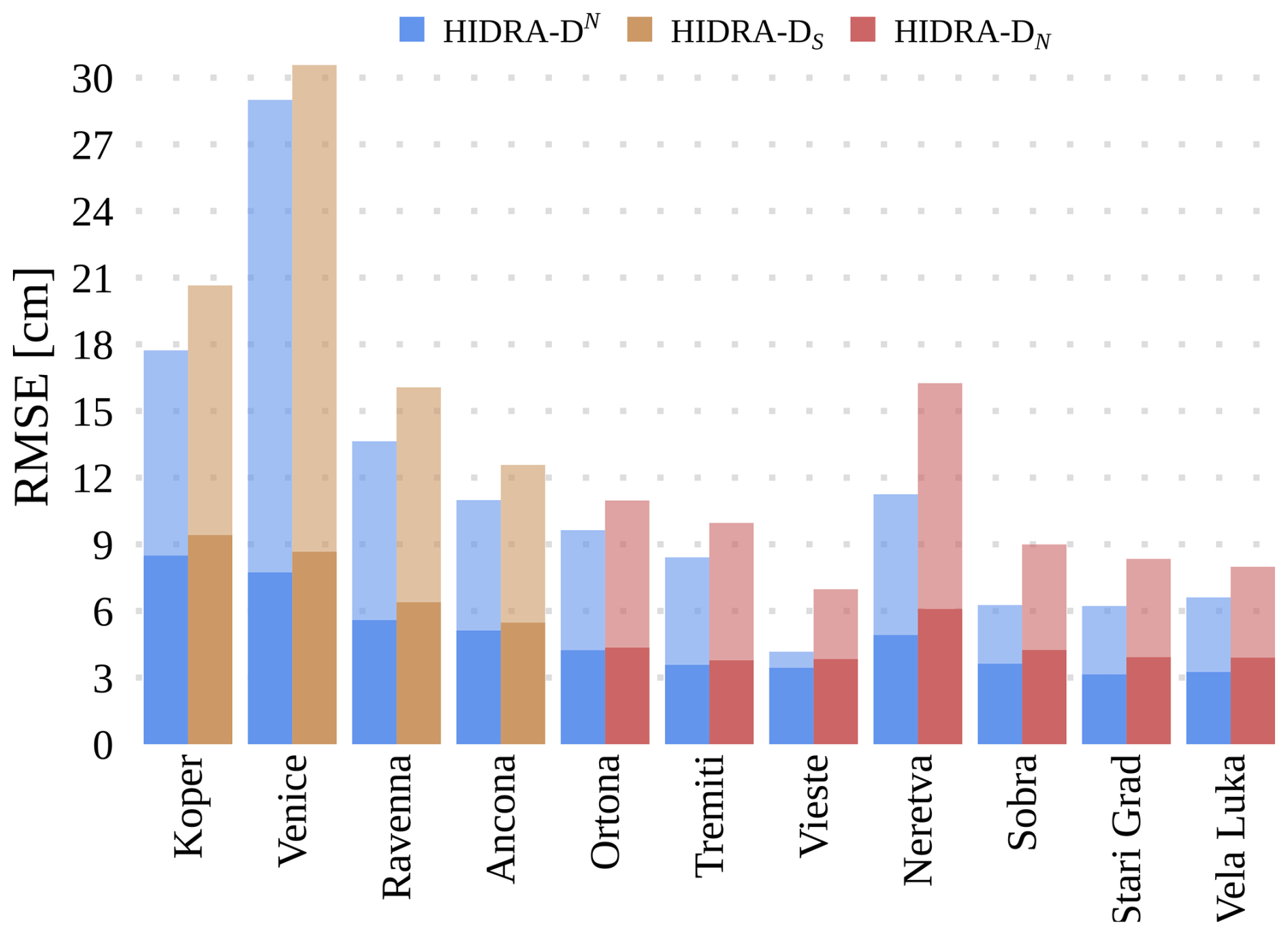
Figure 13 RMSE increase when having only a subset of tide gauges as input. The model HIDRA-D_S is trained using only tide gauges from the southern Adriatic, while HIDRA-D_N is trained using only northern locations. The figure presents RMSE scores for regions that were not included as input during training. Solid regions represent the overall RMSE, while semi-transparent regions indicate the RMSE for high SSH values. The results show that, despite the exclusion of entire regions, the performance degradation remains minimal.

4.5 Influence of the spatial scale threshold

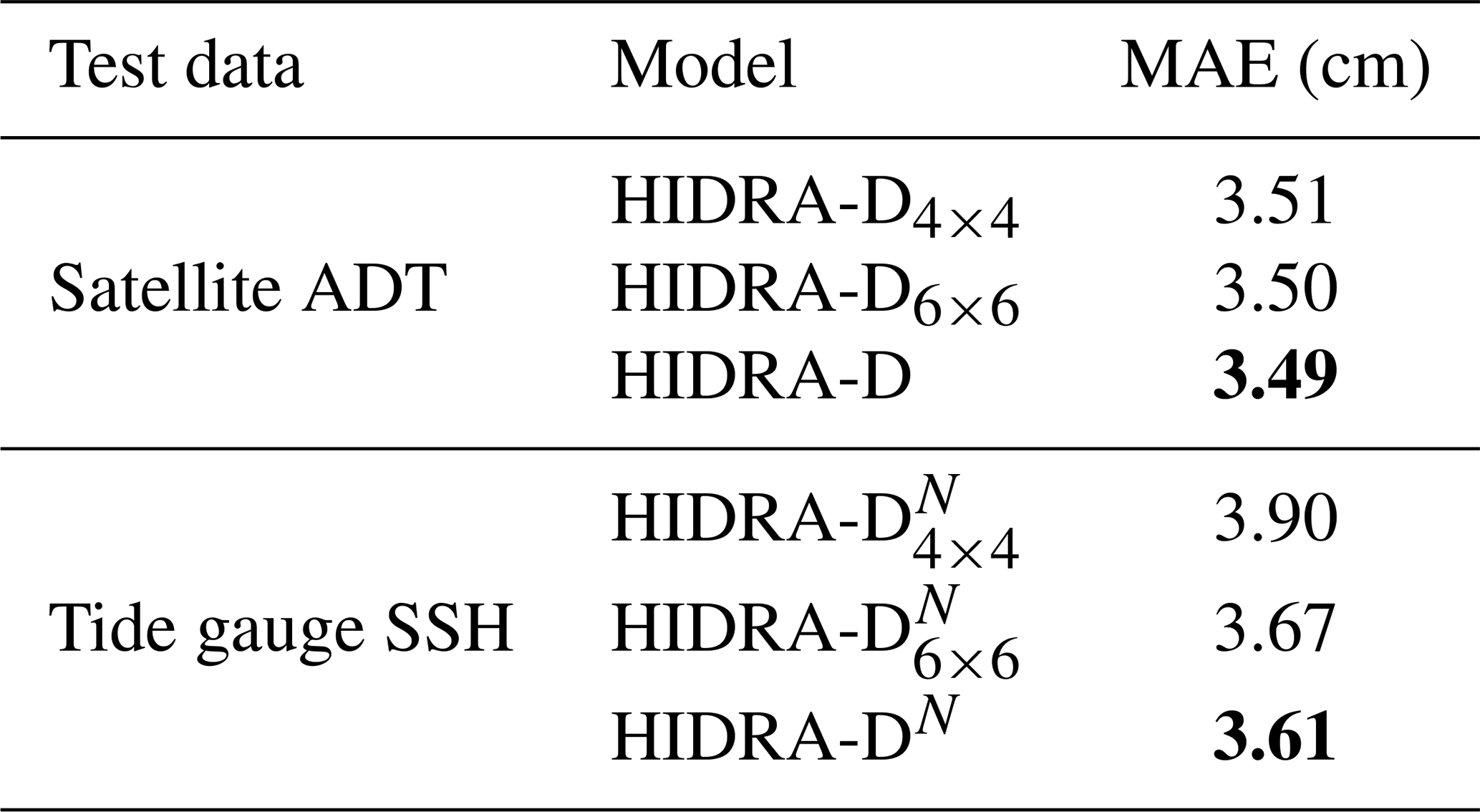
In Sect. 3.2.2, the northern Adriatic barotropic Rossby radius was used to define the spatial scale threshold as λ_R=150 km. This threshold represents the lower limit for the forecasted wavelength in the dense output of HIDRA-D and determines the size of the non-zero element regions in the Fourier matrix F, which for λ_R=150 km corresponds to 5×5 and 4×5 submatrices. To investigate the influence of this hyperparameter, we conducted an ablation study by training two model variants where the dimensions of the predicted Fourier submatrices were increased or decreased by one element in each dimension. This modification required changing the output dimension of the final dense layer to match the number of coefficients in these resized submatrices. Note that the final spatial grid size (94×115) remains unchanged. These variants are hereafter referred to as HIDRA-D_4×4 (utilizing 4×4 and 3×4 submatrices) and HIDRA-D_6×6 (utilizing 6×6 and 5×6 submatrices). For the cross-validation setup, they are denoted as ${\text{HIDRA-D}}_{\mathrm{4}\times \mathrm{4}}^N$ and ${\text{HIDRA-D}}_{\mathrm{6}\times \mathrm{6}}^N$.

The results of this ablation study are presented in Table 5. The evaluation on the satellite ADT measurements shows that the MAE is largely unaffected by changes in the submatrix size. However, a different trend emerges in the cross-validation scenario, where models were evaluated on tide gauges that were excluded from training. In this case, our proposed model HIDRA-D^N, achieved the lowest MAE. This supports our selection of λ_R.

Table 5 Mean absolute error for different spatial scale thresholds, evaluated on satellite ADT measurements and on excluded tide gauge measurements in a cross-validation setup. The best results are highlighted in bold.

5 Conclusions

This paper introduces HIDRA-D, a novel deep learning model for generating dense, two-dimensional sea level forecasts across an entire regional basin, representing a significant development over previous point-prediction models in the HIDRA family. HIDRA-D successfully integrates the HIDRA3 module (Rus et al., 2025d) for point predictions at tide gauge locations with a new Dense decoder module that generates the low-frequency spatial components of the sea level field. Crucially, the model demonstrates a novel methodology for leveraging extremely sparse and unevenly distributed satellite ADT data, combined with tide gauge observations, to achieve accurate two-dimensional basin-scale predictions. A key aspect of this integration is a new procedure for intercalibrating tide gauges and ADT, where the vertical displacement of each tide gauge is estimated as a learnable parameter during the model's training process, enabling the direct use of both satellite ADT and tide gauge SSH data for supervision.

When comparing 3 d forecasts of NEMO and HIDRA-D with satellite ADT measurements in the Adriatic Sea, HIDRA-D achieves a 28.0 % reduction in MAE. This demonstrates that deep learning is a viable, and often more accurate, alternative to computationally expensive numerical models for sea level forecasting. Furthermore, the model exhibits remarkable robustness to a sparse tide gauge network, successfully capturing large-scale dynamics even when trained on remote stations, which is critical for applications in data-sparse regions. However, although HIDRA-D, like NEMO, captures large-scale sea level trends, it struggles to reproduce high-frequency local variations and extreme peaks at untrained coastal locations. The model's performance is highest in open waters but degrades in coastal areas with complex bathymetry, such as Koper and Venice, specifically during extreme sea level events. Consequently, while HIDRA-D offers a computationally efficient alternative for basin-scale forecasting, it currently lags behind traditional numerical models like NEMO for specific applications such as coastal flood warnings at locations where no prior training data is available.

A limitation of data-driven approaches like HIDRA-D, compared to process-based numerical models, is their lack of physical interpretability. Future research will focus on addressing this and other open questions. First, we aim to enhance the model's predictive skill by exploring methods to resolve higher-frequency spatial variations and better capture dynamics in complex coastal regions. Second, we will assess the generalizability of HIDRA-D. While the architecture is general and designed to work for any location, application to new regions requires retraining on local datasets. We note that the HIDRA2 architecture was successfully applied in the Baltic basin along the Estonian coast (Barzandeh et al., 2025), performing well despite being originally developed for the Adriatic. This gives optimism that HIDRA-D would also perform well there, as it is its successor, although this remains to be thoroughly tested. We plan to adapt and evaluate the architecture in other ocean basins with diverse characteristics, such as larger areas, different tidal regimes, and varying data availability, to verify its transferability.

Appendix A: Tide gauge correlations

To assess the redundancy of information provided by the tide gauge network, we computed the Pearson correlation coefficients between the SSH signals of all station pairs. Two distinct clusters with high internal correlation are visible (Fig. A1): the northern Adriatic group (Koper, Venice, Ravenna, Ancona) and the central/southern group.

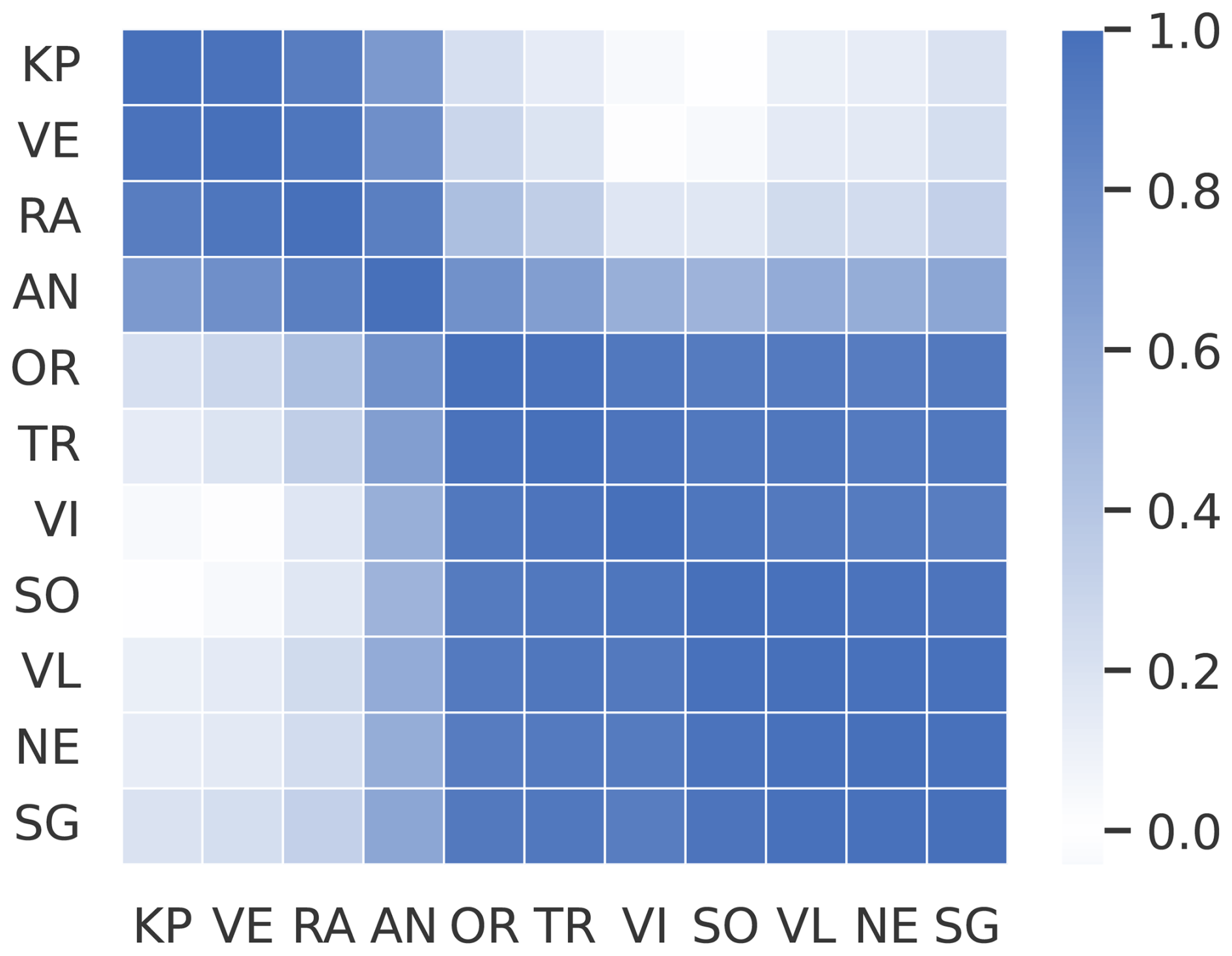
Figure A1 Pearson correlation matrix of SSH measurements between different tide gauge locations. The stations are: Koper (KP), Venice (VE), Ravenna (RA), Ancona (AN), Ortona (OR), Tremiti (TR), Vieste (VI), Sobra (SO), Vela Luka (VL), Neretva (NE), and Stari Grad (SG). Two distinct clusters with high internal correlation are visible: the northern Adriatic group (KP, VE, RA, AN) and the central/southern group.

Appendix B: Additional forecast visualizations

This appendix contains visualizations of model performance under calm atmospheric conditions, complementing the storm surge examples presented in the main text. Figure B1 shows a subset of dense sea level predictions generated by HIDRA-D and NEMO, and Fig. B2 compares dense predictions with tide gauge measurements.

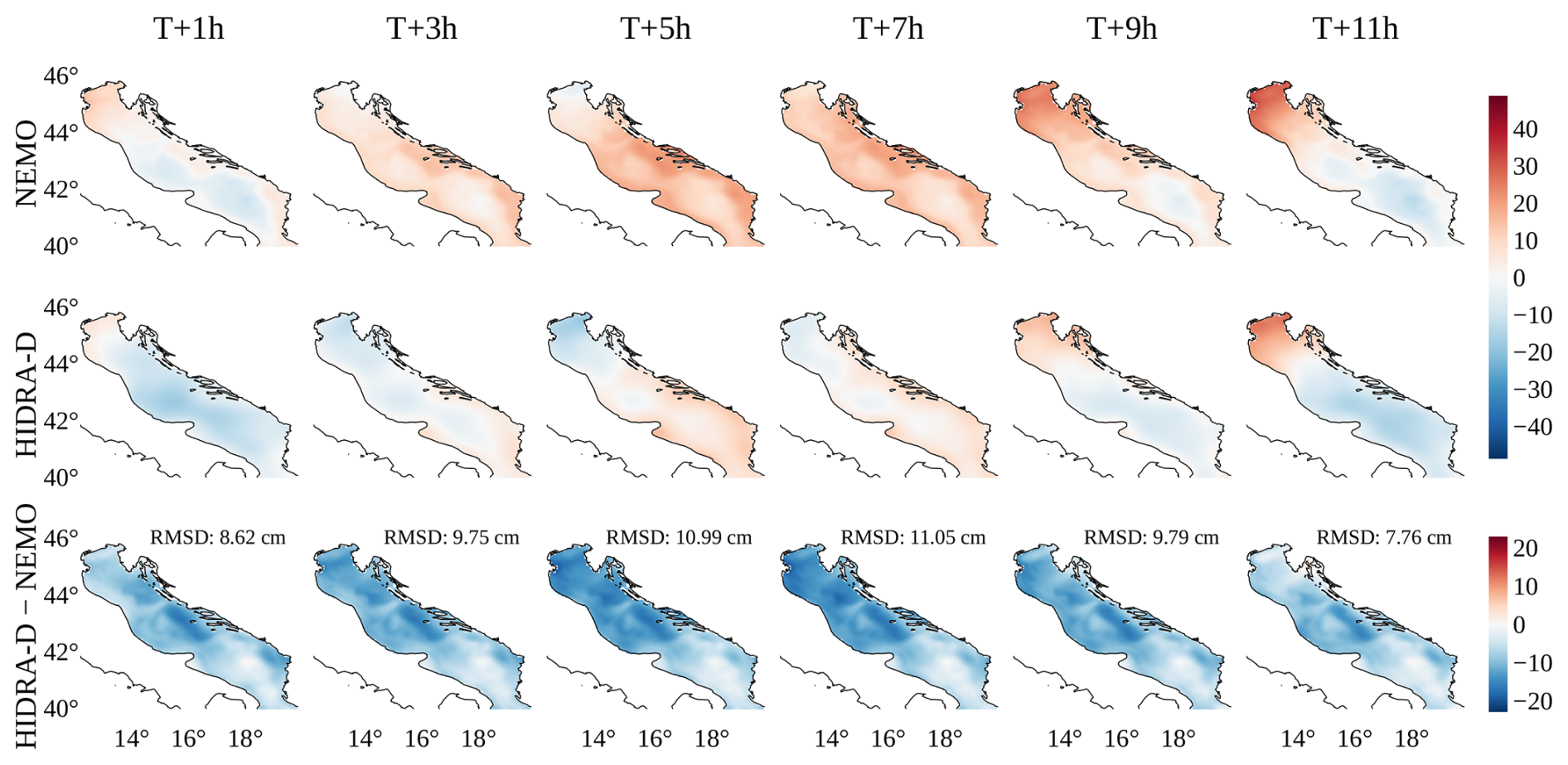
Figure B1 A subset of dense sea level predictions generated by HIDRA-D and NEMO under calm atmospheric conditions. The forecasts correspond to T = 4 November 2020, 23:00 UTC, the units are cm. HIDRA-D produces a spatially smoother forecast compared to NEMO. The bottom row illustrates the difference between HIDRA-D and NEMO; note that it has a separate color bar. The root mean squared difference (RMSD) between the two models is indicated in each panel.

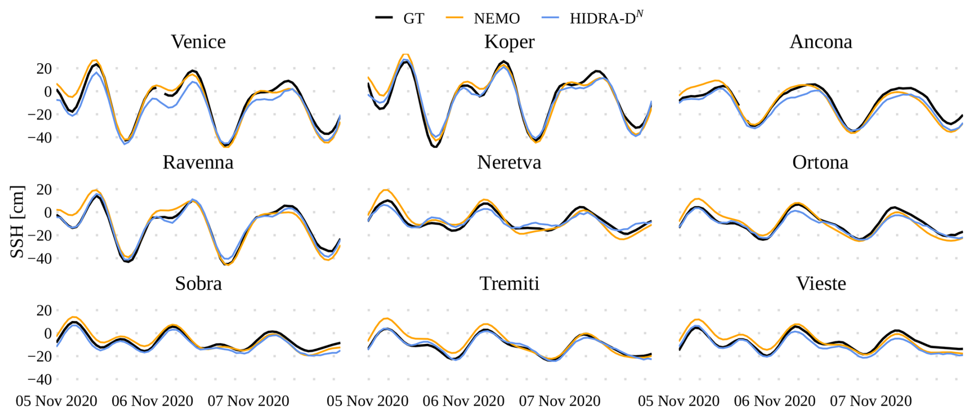
Figure B2 Prediction under calm atmospheric conditions. An example of a single forecast from 4 November 2020, at 23:00 UTC for HIDRA-D^N and NEMO, compared with tide gauge measurements. Note that during training HIDRA-D^N did not see any data from the station on each panel.