The BiogeochemicAl Model for Hypoxic and Benthic Influenced areas: BAMHBI v1.0

This paper describes the ocean BiogeochemicAl Model for Hypoxic and Benthic Influenced areas (BAMHBI). BAMHBI is a moderate complexity marine biogeochemical model that describes the cycling of carbon, nitrogen, phosphorus, silicon and oxygen through the marine foodweb. It involves 22 state variables, extends from bacteria up to mesozooplankton and includes three phytoplankton functional types (PFTs), two zooplankton size-classes, a microbial loop with several classes of detritic materials. Five optional modules are available allowing to extend the model with the explicit modelling of Chlorophyll a (Chl a) in each PFT, benthic degradation, gelatinous dynamics, particles aggregation and the carbonate system. BAMHBI describes the degradation of organic matter according to oxygenation conditions using an approach similar to that used in the sediment to simulate early diagenesis. The model is particularly appropriate for modelling low oxygen environments and the generation of sulfidic waters. An optional benthic module solves the degradation of sedimentary organic matter and the benthic-pelagic fluxes of solutes using an efficient formulation based on meta-modelling.

This paper describes in details model formulations, implementation and coupling with the physics. BAMHBI's code is written in Fortran and can be coupled with many hydrodynamical models. Two case studies of application of BAMHBI in the Black Sea are described. One describes the application of BAMHBI to simulate the biogeochemical dynamics of the northwestern shelf during the eutrophication period. In particular, the ability of BAMHBI to simulate the oxygen dynamics at seasonal and interannual scales is assessed with a focus on the simulation of bottom hypoxia. We highlight the results of the benthic modelling module and its ability to represent benthic-pelagic fluxes. The second case study compares the BAMHBI simulated Chl a, oxygen and nitrate dynamics in the deep sea with respect to biogeochemical Argo.

1 Introduction

Ocean biogeochemical models depict the cycles of essential chemical elements, mostly carbon (C), nitrogen (N), phosphorus (P) and oxygen (O₂), through the marine foodweb, what is often called the “green ocean.” The organic (living and dead) and inorganic forms of ocean materials and their transformation by biogeochemical processes are described with a level of details that differs according to the objectives of the study and the data at hand. Marine biogeochemical models mostly detail the foodweb from bacteria up to mesozooplankton and do not describe the species level. Instead plankton diversity is divided into groups (usually from two up to four) sharing common functional characteristics, the so-called Plankton Functional Types (PFTs). Each PFT aggregates a large number of species into one compartment. During the last three decades, we have had a considerable development of biogeochemical modelling to understand the mechanisms of environmental changes and to improve the quality of prediction. The increase in computing resources and the new knowledge acquired from observations have allowed the development of more complex biogeochemical models that incorporate new compartments, the description of the (un)coupled cycles of several chemical elements, the spectral light propagation, etc. Some of these biogeochemical models are updated regularly, well documented, openly available and used in operational production. This is the case for instance of ERSEM (Butenschön et al., 2016), BFM (Cossarini et al., 2017), PISCES (Aumont et al., 2015) and ERGOM (Daewel et al., 2019).

Here we describe the BiogeochemicAl Model for Hypoxic and Benthic Influenced areas (BAMHBI) that has been developed to simulate oxygen deficient environments and the generation of euxinic waters in the water column and on the bottom. BAMHBI is an intermediate complexity model that represents the cycles of C, N, Si, O₂, P through the pelagic and benthic compartments. BAMHBI is coded to be flexible in terms of model structure by (currently) including five optional modules that explicitly model (1) the Chlorophyll a (Chl a) content of each PFT, (2) the omnivorous and carnivorous gelatinous zooplankton, (3) the carbonate system, (4) the aggregation of organic matter and (5) the benthic compartment. This allows the user to obtain a (simplified) version of the model appropriate for the targeted application. BAMHBI is a stand-alone model that can be coupled with any hydrodynamical model.

BAMHBI has been coupled with GOTM and applied in the Black Sea to simulate the eutrophication period (Grégoire et al., 2008) and biogeochemical cycles (Grégoire and Soetaert, 2010). It has been coupled with the GHER hydrodynamical model to predict the occurrence of seasonal hypoxia over the northwestern shelf (Capet et al., 2013) and benthic-pelagic coupling (Capet et al., 2016). BAMHBI has also been applied to simulate the Ligurian sea ecosystem (Raick et al., 2005, 2006). BAMHBI is online coupled with the hydrodynamical model NEMO in the frame of the Copernicus Marine Service for forecasting (daily production of a 10 d forecast) and hindcasting (back to 1950) the Black Sea's biogeochemistry (Ciliberti et al., 2021).

This paper describes in detail the BAMHBI conceptual and mathematical model. Two applications describe the coupling of BAMHBI with the NEMO hydrodynamical model in a three-dimensional framework.

2 The BAMHBI Model

BAMHBI models trophic interactions across the food web, spanning from bacteria to mesozooplankton throughout both the pelagic and benthic system. The number of state variables varies from 22 in the simplest version of BAMHBI up to 35 in the full version that includes all the optional modules (Fig. 1, Table 1).

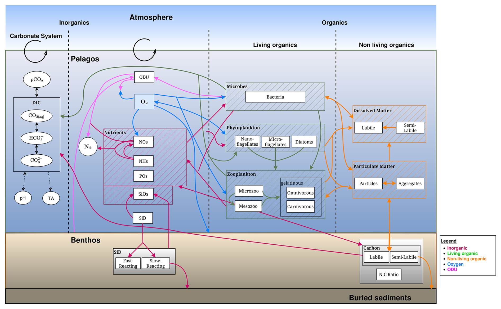
Figure 1 Schematic representation of the BAMHBI biogeochemical model showing the model state variables (in rectangular boxes) and interactions between them in the pelagic and benthic region differentiating the inorganic, living and non-living organic parts which are made of carbon, nitrogen and phosphorus, and also silicon. It also shows the oxygen (O₂) and oxygen demand unit (ODU) fluxes. Optional modules are framed in black: carbonate, benthic, gelatinous, aggregation modules. An additional optional module explicitly computes the Chl a content of each Plankton Functional Type.

The model state variables are listed in Table 1 and the ordinary variables are given in Table 2 and their evolution is governed by the following general equation:

$$\begin{array}{}\text{(1)}& \begin{array}{rl}{\displaystyle \frac{\partial C}{\partial t}}& +\mathit{v}.\mathrm{\nabla }C+{\displaystyle \frac{\partial \left(v_{z,C}C\right)}{\partial z}}\\ & ={\left.{\displaystyle \frac{\partial C}{\partial t}}\right|}_{\text{Bio}}+{\mathrm{\nabla }}_{\mathrm{H}}\left(K_{\mathrm{D}}{\mathrm{\nabla }}_{\mathrm{H}}C\right)+{\displaystyle \frac{\partial }{\partial z}}{\mathit{\lambda }}^C{\displaystyle \frac{\partial C}{\partial z}}\end{array}\end{array}$$

Equation (1) expresses that the rate of change of each concentration of biogeochemical component C, expressed in mmol m⁻³, results from the three-dimensional transport by advection (v.∇C) by the main current with a velocity v, sinking ($\frac{\partial \left(v_{z,C}C\right)}{\partial z}$) with a sinking velocity v_z,C, diffusion (${\mathrm{\nabla }}_{\mathrm{H}}\left(K_{\mathrm{D}}{\mathrm{\nabla }}_{\mathrm{H}}C\right)+\frac{\partial }{\partial z}{\mathit{\lambda }}^C\frac{\partial C}{\partial z}$) with a vertical and horizontal diffusion coefficients respectively of λ^C and K_D and biogeochemical interactions ($\frac{\partial C}{\partial t}{|}_{\text{Bio}}$). Equations (2) until (25) give the biogeochemical interactions for each state variable listed in Table 1. In these equations, the subscript i refers to the three phytoplankton functional groups ($i=\mathrm{1},\mathrm{2},\mathrm{3}$) while j refers to the two zooplankton (gelatinous) groups ($j=\mathrm{1},\mathrm{2}$).

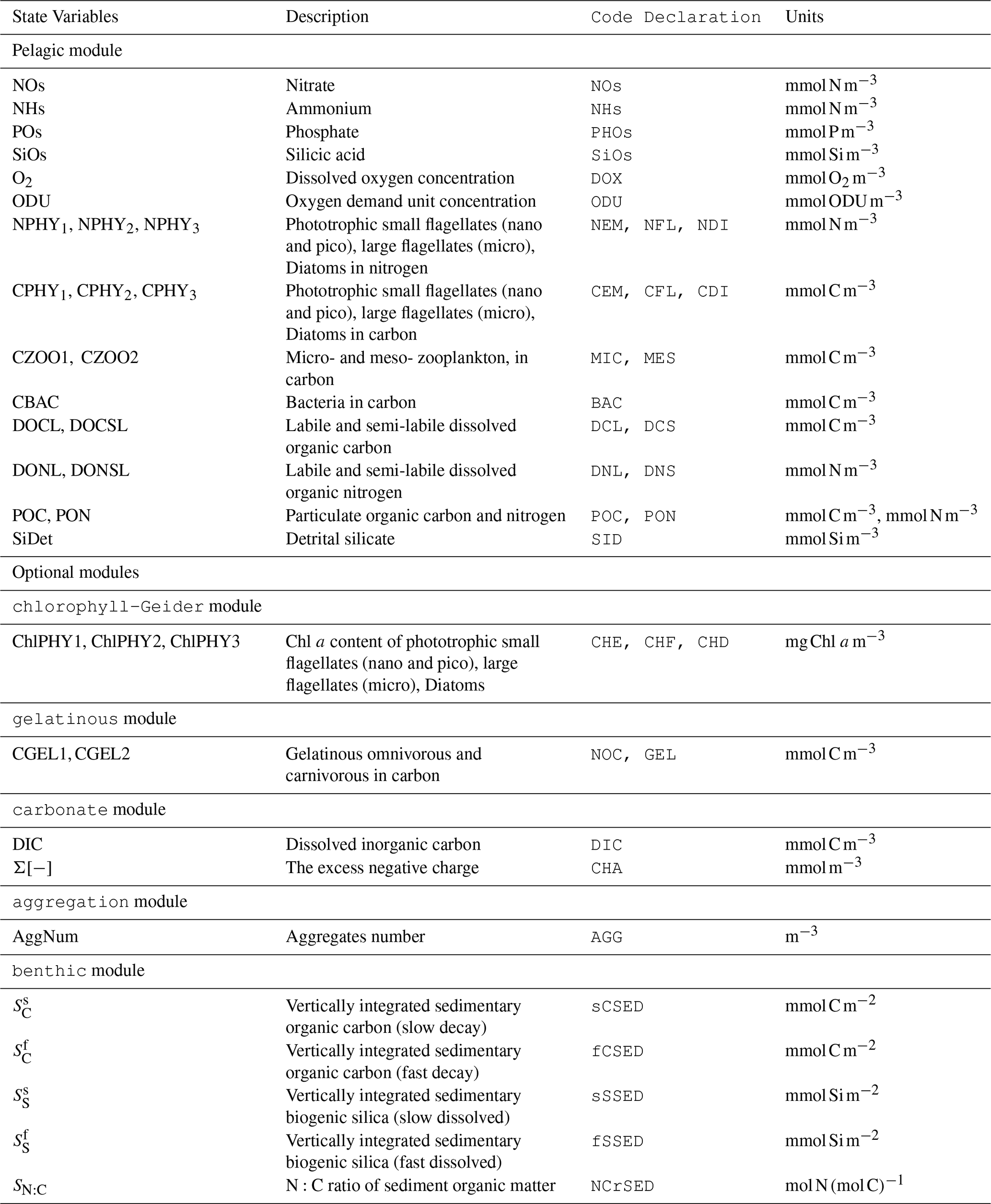
Table 1 List of biogeochemical state variables, description, code declaration and units.

$$\begin{array}{ll}{\displaystyle }& {\displaystyle }{\left.{\displaystyle \frac{\partial {\text{CPHY}}_i}{\partial t}}\right|}_{\text{Bio}}={\text{PhotosynthesisPHY}}_i\\ {\displaystyle }& {\displaystyle }-{\text{RespirationPHY}}_i-{\text{LeakagePHY}}_{\mathrm{C},i}\\ \text{(2)}& {\displaystyle }& {\displaystyle }-{\text{MortPHY}}_{\mathrm{C},i}-{\text{Graz}}_{{\text{CPHY}}_i}(i=\mathrm{1},\mathrm{2},\mathrm{3}){\displaystyle }& {\displaystyle }{\left.{\displaystyle \frac{\partial {\text{NPHY}}_i}{\partial t}}\right|}_{\text{Bio}}=({\mathrm{NOs}}_i^{\mathrm{uptake}}+{\mathrm{NHs}}_i^{\mathrm{uptake}})-{\text{LeakagePHY}}_{\mathrm{N},i}\\ \text{(3)}& {\displaystyle }& {\displaystyle }-{\text{MortPHY}}_{\mathrm{N},i}-{\text{Graz}}_{{\text{NPHY}}_i}(i=\mathrm{1},\mathrm{2},\mathrm{3}){\displaystyle }& {\displaystyle }{\left.{\displaystyle \frac{\partial {\text{CZOO}}_j}{\partial t}}\right|}_{\text{Bio}}={\text{GrowthZOO}}_{\mathrm{C},j}\\ \text{(4)}& {\displaystyle }& {\displaystyle }-{\text{MortZOO}}_{\mathrm{C},j}-{\text{Graz}}_{{\text{CZOO}}_j}(j=\mathrm{1},\mathrm{2})\text{(5)}& {\displaystyle }& {\displaystyle }{\left.{\displaystyle \frac{\partial \text{CBAC}}{\partial t}}\right|}_{\text{Bio}}=\text{GrowthBAC}-{\text{MortBAC}}_{\mathrm{C}}-{\text{Graz}}_{\mathrm{CBAC}}{\displaystyle }& {\displaystyle }{\left.{\displaystyle \frac{\partial \mathrm{NOs}}{\partial t}}\right|}_{\text{Bio}}=-\sum _{j=\mathrm{1}}^{\mathrm{3}}{\mathrm{NOs}}_j^{\mathrm{uptake}}+{\mathrm{NHsoxid}}_{{\mathrm{O}}_{\mathrm{2}}}\text{NHs}\\ {\displaystyle }& {\displaystyle }-\text{RespBACNitrate}{\mathit{\gamma }}_{\mathrm{NOs}}^{\mathrm{POC}}-\text{NHs}{\mathrm{oxid}}_{\mathrm{NOs}}\text{NHs}{\mathit{\gamma }}_{\mathrm{NOs}}^{\mathrm{NHs}}\\ \text{(6)}& {\displaystyle }& {\displaystyle }-{\text{ODUoxid}}_{\mathrm{NOs}}\mathrm{ODU}{\mathit{\gamma }}_{\mathrm{NOs}}^{\mathrm{ODU}}{\displaystyle }& {\displaystyle }{\left.{\displaystyle \frac{\partial \mathrm{NHs}}{\partial t}}\right|}_{\text{Bio}}=\sum _{j=\mathrm{1}}^{\mathrm{2}}\left({\text{ExcrZOO}}_j\right)+\mathrm{ExcrBAC}\\ {\displaystyle }& {\displaystyle }-\sum _{j=\mathrm{1}}^{\mathrm{3}}{\mathrm{NHs}}_j^{\mathrm{uptake}}-U_{\mathrm{A}}-\text{NHs}{\mathrm{oxid}}_{\mathrm{NOs}}\text{NHs}\\ \text{(7)}& {\displaystyle }& {\displaystyle }-\text{NHs}{\mathrm{oxid}}_{{\mathrm{O}}_{\mathrm{2}}}\text{NHs}{\displaystyle }& {\displaystyle }\text{if}\mathtt{\text{Gelatinous :}}+\sum _{j=\mathrm{1}}^{\mathrm{2}}\left({\text{AdjExcrGEL}}_j\right)\\ {\displaystyle }& {\displaystyle }{\left.{\displaystyle \frac{\partial \mathrm{POs}}{\partial t}}\right|}_{\text{Bio}}=\left[\sum _{j=\mathrm{1}}^{\mathrm{2}}\left({\text{ExcrZOO}}_j\right)+\mathrm{ExcrBAC}-U_{\mathrm{A}}\right]\\ \text{(8)}& {\displaystyle }& {\displaystyle }\left(\mathrm{P}:\mathrm{N}\right)-\sum _{j=\mathrm{1}}^{\mathrm{3}}{\mathrm{POs}}_j^{\mathrm{uptake}}-\mathrm{PrecipitationPOs}{\displaystyle }& {\displaystyle }\text{if}\mathtt{\text{Gelatinous :}}+\sum _{j=\mathrm{1}}^{\mathrm{2}}\left({\text{AdjExcrGEL}}_j\right)\\ \text{(9)}& {\displaystyle }& {\displaystyle }{\left.{\displaystyle \frac{\partial \mathrm{SiOs}}{\partial t}}\right|}_{\text{Bio}}=-{\text{SiOs}}^{\mathrm{uptake}}+\text{DissolutionSiDet}{\displaystyle }& {\displaystyle }{\left.{\displaystyle \frac{\partial \mathrm{DOCL}}{\partial t}}\right|}_{\text{Bio}}=\sum _{i=\mathrm{1}}^{\mathrm{3}}({\text{LeakagePHY}}_{\mathrm{C},i}\\ {\displaystyle }& {\displaystyle }+{\mathit{\gamma }}_{\mathrm{1}}{\text{ExtraExcrPHY}}_i+(\mathrm{1}-{\mathit{\gamma }}_{\mathrm{1}}){\mathit{\delta }}_{\mathrm{2}}{\text{ExtraExcrPHY}}_i)\\ {\displaystyle }& {\displaystyle }+\mathrm{HydrolDOCSL}-U_c\\ {\displaystyle }& {\displaystyle }+{\mathit{\delta }}_{\mathrm{1}}\left[\mathit{ϵ}\sum _{i=\mathrm{1}}^{\mathrm{3}}{\text{MortPHY}}_{\mathrm{C},i}+{\mathit{\varphi }}_i\sum _{j=\mathrm{1}}^{\mathrm{2}}{\text{GrazZOO}}_{\mathrm{C},j}\right.\\ \text{(10)}& {\displaystyle }& {\displaystyle }\left.+{\text{MortBAC}}_{\mathrm{C}}+\mathrm{HydrolPOC}\right]{\displaystyle }& {\displaystyle }{\left.{\displaystyle \frac{\partial \mathrm{DONL}}{\partial t}}\right|}_{\text{Bio}}=\sum _{i=\mathrm{1}}^{\mathrm{3}}\left({\text{LeakagePHY}}_{\mathrm{N},i}\right)\\ {\displaystyle }& {\displaystyle }+{\mathit{\delta }}_{\mathrm{1}}\left[\mathit{ϵ}\sum _{i=\mathrm{1}}^{\mathrm{3}}{\text{MortPHY}}_{\mathrm{N},i}+\mathit{\varphi }\sum _{j=\mathrm{1}}^{\mathrm{2}}{\text{GrazZOO}}_{\mathrm{N},j}\right.\\ {\displaystyle }& {\displaystyle }\left.+{\displaystyle \frac{{\text{MortBAC}}_{\mathrm{C}}}{(\mathrm{C}:\mathrm{N}{)}_{\mathrm{BAC}}}}+\mathrm{HydrolPON}\right]+\mathrm{HydrolDONSL}\\ \text{(11)}& {\displaystyle }& {\displaystyle }-U_n{\displaystyle }& {\displaystyle }{\left.{\displaystyle \frac{\partial \mathrm{DOCSL}}{\partial t}}\right|}_{\text{Bio}}=\sum _{i=\mathrm{1}}^{\mathrm{3}}\left((\mathrm{1}-{\mathit{\gamma }}_{\mathrm{1}})(\mathrm{1}-{\mathit{\delta }}_{\mathrm{2}}){\text{ExtraExcrPHY}}_i\right)\\ {\displaystyle }& {\displaystyle }+(\mathrm{1}-{\mathit{\delta }}_{\mathrm{1}})\left[\mathit{ϵ}\sum _{i=\mathrm{1}}^{\mathrm{3}}{\text{MortPHY}}_{\mathrm{C},i}+\mathit{\varphi }\sum _{j=\mathrm{1}}^{\mathrm{2}}{\text{GrazZOO}}_{\mathrm{C},j}\right.\\ \text{(12)}& {\displaystyle }& {\displaystyle }\left.+\mathrm{HydrolPOC}+{\text{MortBAC}}_{\mathrm{C}}\right]-\mathrm{HydrolDOCSL}{\displaystyle }& {\displaystyle }{\left.{\displaystyle \frac{\partial \mathrm{DONSL}}{\partial t}}\right|}_{\text{Bio}}=(\mathrm{1}-{\mathit{\delta }}_{\mathrm{1}})\left[\mathit{ϵ}\sum _{i=\mathrm{1}}^{\mathrm{3}}{\text{MortPHY}}_{\mathrm{N},i}\right.\\ {\displaystyle }& {\displaystyle }\left.+\mathit{\varphi }\sum _{j=\mathrm{1}}^{\mathrm{2}}{\text{GrazZOO}}_{\mathrm{N},j}+\mathrm{HydrolPON}+{\displaystyle \frac{{\text{MortBAC}}_{\mathrm{C}}}{(\mathrm{C}:\mathrm{N}{)}_{\mathrm{BAC}}}}\right]\\ \text{(13)}& {\displaystyle }& {\displaystyle }-\mathrm{HydrolDONSL}{\displaystyle }& {\displaystyle }{\left.{\displaystyle \frac{\partial \mathrm{POC}}{\partial t}}\right|}_{\text{Bio}}=\sum _{i=\mathrm{1}}^{\mathrm{3}}(\mathrm{1}-\mathit{ϵ}){\text{MortPHY}}_{\mathrm{C},i}\\ {\displaystyle }& {\displaystyle }+\sum _{j=\mathrm{1}}^{\mathrm{2}}\left({\text{MortZOO}}_{\mathrm{C},j}+{\mathrm{MortGEL}}_{\mathrm{C},j}\right)\\ \text{(14)}& {\displaystyle }& {\displaystyle }+\sum _{j=\mathrm{1}}^{\mathrm{2}}\left((\mathrm{1}-{\mathit{\beta }}_{\mathrm{C}})I_{\mathrm{C},j}\right)-\mathrm{HydrolPOC}-{\text{Graz}}_{\mathrm{POC}}{\displaystyle }& {\displaystyle }\text{if}\mathtt{\text{Gelatinous :}}\\ {\displaystyle }& {\displaystyle }+\sum _{j=\mathrm{1}}^{\mathrm{2}}\left((\mathrm{1}-{\text{AssEffGEL}}_j){\mathrm{GrazGEL}}_{\mathrm{C},j}\right)\\ {\displaystyle }& {\displaystyle }{\left.{\displaystyle \frac{\partial \mathrm{PON}}{\partial t}}\right|}_{\text{Bio}}=\sum _{i=\mathrm{1}}^{\mathrm{3}}(\mathrm{1}-\mathit{ϵ}){\text{MortPHY}}_{\mathrm{N},i}\\ {\displaystyle }& {\displaystyle }+\sum _{j=\mathrm{1}}^{\mathrm{2}}\left({\displaystyle \frac{{\text{MortZOO}}_{\mathrm{C},j}}{(\mathrm{C}:\mathrm{N}{)}_{{\mathrm{ZOO}}_j}}}+{\displaystyle \frac{{\mathrm{MortGEL}}_{\mathrm{C},j}}{(\mathrm{C}:\mathrm{N}{)}_{{\mathrm{GEL}}_j}}}\right.\\ \text{(15)}& {\displaystyle }& {\displaystyle }\left.+(\mathrm{1}-{\mathit{\beta }}_N)I_{\mathrm{N},j}\right)-\mathrm{HydrolPON}-{\text{Graz}}_{\mathrm{PON}}{\displaystyle }& {\displaystyle }\text{if}\mathtt{\text{Gelatinous :}}\\ {\displaystyle }& {\displaystyle }+\sum _{j=\mathrm{1}}^{\mathrm{2}}\left((\mathrm{1}-{\mathrm{AssEffGEL}}_j){\mathrm{GrazGEL}}_{\mathrm{N},j}\right)\\ {\displaystyle }& {\displaystyle }{\left.{\displaystyle \frac{\partial \mathrm{SiDet}}{\partial t}}\right|}_{\text{Bio}}=-\text{DissolutionSiDet}\\ \text{(16)}& {\displaystyle }& {\displaystyle }+({\text{MortPHY}}_{\mathrm{N},\mathrm{3}}+{\text{Graz}}_{{\text{NPHY}}_{\mathrm{3}}})(\mathrm{Si}:\mathrm{N}{)}_{{\mathrm{PHY}}_{\mathrm{3}}}{\displaystyle }& {\displaystyle }{\left.{\displaystyle \frac{\partial \mathrm{ODU}}{\partial t}}\right|}_{\text{Bio}}={\mathit{\gamma }}_{\mathrm{ODU}}^{\mathrm{POC}}\mathrm{AnoxicRespBAC}\\ {\displaystyle }& {\displaystyle }-{\text{ODUoxid}}_{\mathrm{NOs}}\mathrm{ODU}-{\text{ODUoxid}}_{{\mathrm{O}}_{\mathrm{2}}}\mathrm{ODU}\\ \text{(17)}& {\displaystyle }& {\displaystyle }-\mathrm{SolidODU}{\displaystyle }& {\displaystyle }{\left.{\displaystyle \frac{\partial {\mathrm{O}}_{\mathrm{2}}}{\partial t}}\right|}_{\text{Bio}}=\sum _{i=\mathrm{1}}^{\mathrm{3}}({\text{PhotosynthesisPHY}}_i\\ {\displaystyle }& {\displaystyle }+{\text{ExtraExcrPHY}}_i){\mathit{\gamma }}_{{\mathrm{O}}_{\mathrm{2}}}^{\mathrm{C}}-\sum _{j=\mathrm{1}}^{\mathrm{2}}({\mathrm{RespZOO}}_j){\mathit{\gamma }}_{{\mathrm{O}}_{\mathrm{2}}}^{\mathrm{C}}\\ {\displaystyle }& {\displaystyle }-\mathrm{RespBACOxygen}{\mathit{\gamma }}_{{\mathrm{O}}_{\mathrm{2}}}^{\mathrm{C}}-\text{NHs}{\mathrm{oxid}}_{{\mathrm{O}}_{\mathrm{2}}}\text{NHs}{\mathit{\gamma }}_{{\mathrm{O}}_{\mathrm{2}}}^{\mathrm{NHs}}\\ \text{(18)}& {\displaystyle }& {\displaystyle }-{\text{ODUoxid}}_{{\mathrm{O}}_{\mathrm{2}}}\mathrm{ODU}{\mathit{\gamma }}_{{\mathrm{O}}_{\mathrm{2}}}^{\mathrm{ODU}}{\displaystyle }& {\displaystyle }\text{if}\mathtt{\text{Gelatinous :}}\\ {\displaystyle }& {\displaystyle }-\sum _{j=\mathrm{1}}^{\mathrm{2}}({\mathrm{RespGEL}}_j+{\mathrm{AdjRespGEL}}_j){\mathit{\gamma }}_{{\mathrm{O}}_{\mathrm{2}}}^{\mathrm{C}}\end{array}$$

Optional modules

Chlorophyll-Geider module

$$\begin{array}{ll}{\displaystyle }& {\displaystyle }{\left.{\displaystyle \frac{\partial {\mathrm{ChlPHY}}_i}{\partial t}}\right|}_{\text{Bio}}=\mathrm{SynthesisChlPHY}i\\ {\displaystyle }& {\displaystyle }-{\mathrm{RespirationChlPHY}}_i-{\mathrm{MortChlPHY}}_i\\ \text{(19)}& {\displaystyle }& {\displaystyle }-{\text{Graz}}_{{\mathrm{ChlPHY}}_i}(i=\mathrm{1},\mathrm{2},\mathrm{3})\end{array}$$

Gelatinous module

$$\begin{array}{ll}{\displaystyle }& {\displaystyle }{\left.{\displaystyle \frac{\partial {\mathrm{CGEL}}_j}{\partial t}}\right|}_{\text{Bio}}={\mathrm{GrowthGEL}}_{\mathrm{C},j}-{\mathrm{MortGEL}}_{\mathrm{C},j}\\ \text{(20)}& {\displaystyle }& {\displaystyle }-{\mathrm{AdjRespGEL}}_j(j=\mathrm{1},\mathrm{2})\end{array}$$

Carbonate module

$$\begin{array}{ll}{\displaystyle }& {\displaystyle }{\left.{\displaystyle \frac{\partial \mathrm{DIC}}{\partial t}}\right|}_{\text{Bio}}=\sum _{j=\mathrm{1}}^{\mathrm{2}}\left({\mathrm{RespZOO}}_j\right)+\\ {\displaystyle }& {\displaystyle }\sum _{j=\mathrm{1}}^{\mathrm{3}}\left(-{\mathrm{GrowthPHY}}_j-{\text{ExtraExcrPHY}}_i\right)\\ \text{(21)}& {\displaystyle }& {\displaystyle }+\mathrm{RespBAC}{\displaystyle }& {\displaystyle }\text{if}\mathtt{\text{Gelatinous :}}+\sum _{j=\mathrm{1}}^{\mathrm{2}}\left({\mathrm{RespGEL}}_j+\mathrm{AdjRespGELj}\right)\\ \text{(22)}& {\displaystyle }& {\displaystyle }{\left.{\displaystyle \frac{\partial \mathrm{\Sigma }[-]}{\partial t}}\right|}_{\text{Bio}}=\mathrm{0}\end{array}$$

Aggregation module

$$\begin{array}{}\text{(23)}& {\displaystyle }{\displaystyle }{\left.{\displaystyle \frac{\partial \mathrm{AggNum}}{\partial t}}\right|}_{\text{Bio}}={\left.{\displaystyle \frac{\partial \mathrm{PON}}{\partial t}}\right|}_{\text{Bio}}{\displaystyle \frac{\mathrm{AggNum}}{\mathrm{PON}}}-\text{Aggregation}\end{array}$$

Benthic module

$$\begin{array}{ll}{\displaystyle }& {\displaystyle \frac{d{S}_i^j}{\mathrm{d}t}}=P_i^j-D_i^j-B_i^j\text{with}i=\mathrm{C},\mathrm{Si}\\ \text{(24)}& {\displaystyle }& {\displaystyle }\text{and}j=f,s\text{fast (f) and slowly (s) degraded}{\displaystyle }& {\displaystyle \frac{d{S}_{\mathrm{N}:\mathrm{C}}}{\mathrm{d}t}}={\displaystyle \frac{d}{\mathrm{d}t}}\left({\displaystyle \frac{S_{\mathrm{N}}}{S_{\mathrm{C}}}}\right)={\displaystyle \frac{\mathrm{1}}{S_{\mathrm{C}}^{\mathrm{2}}}}\left(S_{\mathrm{C}}{\displaystyle \frac{d{S}_{\mathrm{N}}}{\mathrm{d}t}}-S_{\mathrm{N}}{\displaystyle \frac{d{S}_{\mathrm{C}}}{\mathrm{d}t}}\right),\\ {\displaystyle }& {\displaystyle }\text{with}{S}_{\mathrm{C}}=S_{\mathrm{C}}^{\mathrm{s}}+S_{\mathrm{C}}^{\mathrm{f}}\text{and}{S}_{\mathrm{N}}=S_{\mathrm{N}}^{\mathrm{s}}+S_{\mathrm{N}}^{\mathrm{f}}\\ {\displaystyle }& {\displaystyle }={\displaystyle \frac{\mathrm{1}}{S_{\mathrm{C}}}}\left[\right(P_{\mathrm{N}}-D_{\mathrm{N}}-B_{\mathrm{C}}.S_{\mathrm{N}:\mathrm{C}})-S_{\mathrm{N}:\mathrm{C}}(P_{\mathrm{C}}-D_{\mathrm{C}}-B_{\mathrm{C}}\left)\right],\\ {\displaystyle }& {\displaystyle }\text{with}{D}_{\mathrm{C}}=D_{\mathrm{C}}^{\mathrm{s}}+D_{\mathrm{C}}^{\mathrm{f}}\text{and}{P}_{\mathrm{C}}=P_{\mathrm{C}}^{\mathrm{s}}+P_{\mathrm{C}}^{\mathrm{f}}\\ \text{(25)}& {\displaystyle }& {\displaystyle }={\displaystyle \frac{\mathrm{1}}{S_{\mathrm{C}}}}\left[\right(P_{\mathrm{N}}-S_{\mathrm{N}:\mathrm{C}}{P}_{\mathrm{C}}\left)\right]\end{array}$$

Table 2 List of model ordinary variables.

2.1 The pelagic model

The pelagic part describes the foodweb from bacteria up to mesozooplankton and includes three groups of phytoplankton: diatoms, small and large phototrophic flagellates, two zooplankton groups: micro- and mesozooplankton, an explicit representation of the bacterial loop: bacteria, labile and semi-labile dissolved organic matter, particulate organic matter. Each organic variable is described by its carbon content, except the three groups of phytoplankton, dissolved and particulate detritus that are described by their carbon and nitrogen content. The N:P and, in the case of diatoms, the N:Si ratios are assumed constant. In addition, an optional module allows to explicitly model the Chl a content of each phytoplankton group (see Sect. 2.2.1).

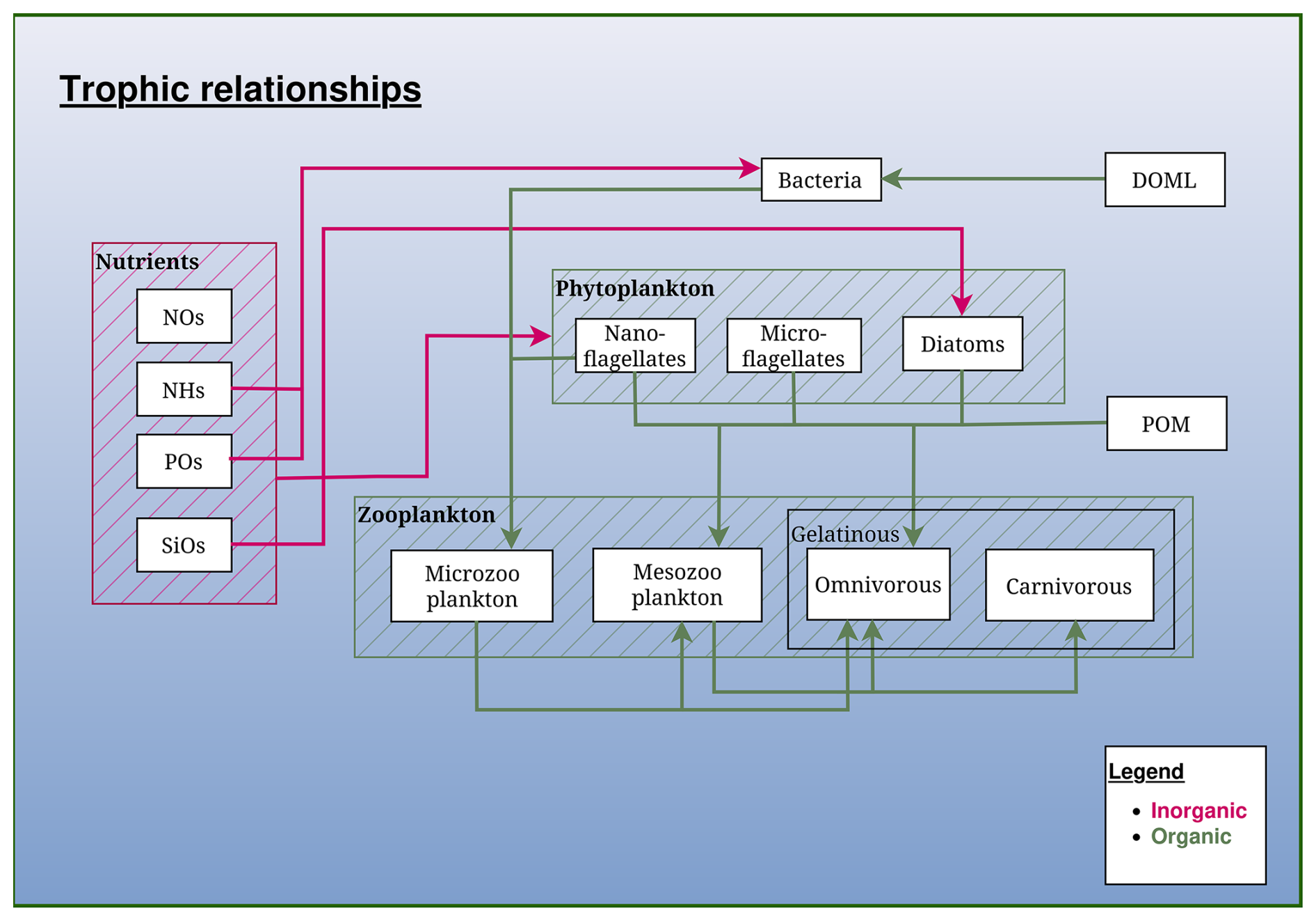
Figure 2 Schematic representation of the trophic relationships in the BAMHBI biogeochemical model. It shows the model state variables (in rectangular boxes) and interactions between them differentiating the inorganic and organic flows made of carbon, nitrogen and phosphorus. The optional gelatinous module is framed in black.

2.1.1 The optical part

The Photosynthetically Active Radiation (PAR) is the fraction of radiation between 400 and 700 nm that can be used by autotrophs for photosynthesis. The sea surface PAR, PAR₀, is obtained from the solar radiation reaching the sea surface, Q_s,0 after removing the reflected (albedo) and infrared (p_IR) fractions (Eq. 27). The vertical penetration of PAR with depth is governed by the Inherent Optical Properties (IOPs) of the medium described here by the absorption (a) and (back)scattering (b) by the optically active components, i.e., here water, phytoplankton and particulate organic carbon (Eqs. 28, 31 and 32). The absorption and scattering of light are constant for pure sea water (Smith and Baker, 1981), while for dead particles (Neukermans et al., 2012) and phytoplankton, they are represented as the product of a specific rate and the concentration of the optically active component. In the case of phytoplankton, the specific absorption coefficient varies according to a power law of total chlorophyll concentration (Bricaud et al., 1995) while for the backscattering the effect of the three phytoplankton groups is differentiated (Vaillancourt et al., 2004). In addition, the effect of the Coloured Dissolved Organic Matter (CDOM) on light absorption is parameterized based on salinity (Kowalczuk et al., 2003; Mobley et al., 2004; Xu et al., 2005). The attenuation coefficients (k) are then computed using the formulations of Lee et al. (2005) (Eq. 29). The model does not describe the spectral composition of the light field but rather differentiates two bands of wavelengths of PAR: a short [i.e., 400–540 nm] and a long [i.e., 540–700 nm] wavelengths bands. For each of these two bands, the IOPs are computed using Eqs. (31) and (32) using the parameters listed in Table 6 and adapted to our case study, the Black Sea, according to Dmitriev et al. (2009). The comparison of the model with in-situ data is described in Macé et al. (2025b).

2.1.2 The autotrophs

The primary producers are divided into three functional groups. The small flagellates lumping the pico-and nanophytoplankton constitute the first group. This group is characterized by high nutrients affinity due to their large surface to volume ratio, high photosynthetic efficiency, high growth and nutrient uptake rates. Large flagellates are lumped into the second group characterized by a high requirement for nutrients, low photosynthetic efficiency and growth rate. The phytoplankton silicifiers (e.g. diatoms) that convert dissolved silicate to particulate silicate and then contribute to the silicate pumping in surface waters constitute the third group. Each group is described by two state variables representing their N and C content. Phytoplankton N:C ratios vary around the Redfield ratio, between the limits (N:C)${}_{\mathrm{PHY},min}$ and (N:C)_PHY,max. The phytoplankton N uptake and photosynthesis are modelled according to the model described in Tett (1998) and Smith and Tett (2000) which is based on the “cell–quota, threshold–limitation” algal growth model of Droop (1983) accounting for the potential control of growth by several nutrients and light. With this formulation, photosynthesis increases with the light availability, the N:C and Chl a:C ratios are zero when the N:C ratio reaches its minimum value or when there is no light (Eq. 33).

Phytoplankton respiration consists of a basal and activity respiration (Eq. 34). Phytoplankton excretion is the sum of two processes: leakage and active release (Eq. 35). As in Anderson and Pondaven (2003), we assume that a constant fraction, (parameter γ₁), of all carbon fixed by photosynthesis is leaked from plant cells. In addition, metabolic instabilities in algae, for example, caused by shifts in environmental factors (light, nutrients) cause “extra” carbon to be excreted by phytoplankton (Mague et al., 1980; Williams, 1990). This production of extra carbon is considered as an “overflow” of photosynthesis under nutrient limitation and, thus, is calculated as a fraction (parameter γ₂) of the difference between the nutrient-limited (actual C:N ratio) and nutrient saturated (minimum C:N ratio) growth rate as in Anderson and Pondaven (2003) and Van den Meersche et al. (2004) (Eq. 35). A fraction (parameter γ₁) of this carbon extra excretion is leaked from the cells and is exported towards the labile DOC (Eq. 10), while the remainder (1−γ₁) is actively released and is partitioned between the labile (parameter δ₂) and semi-labile (1−δ₂) DOC (Anderson and Pondaven, 2003) (Eqs. 10 and 12).

Inorganic nitrogen can be taken in excess with respect to their immediate need for growth. The luxury uptake is stored and available for later use. For each phytoplankton group, the N:P and N:Si ratios are assumed constant following the Redfield hypothesis and the exchanges of N, P and Si are maintained in balance. The inorganic nutrient uptake increases at low phytoplankton Nut:C (Nut being N, P or Si) ratios and stops when the Nut:C ratio reaches a maximum value. It is not affected by the light intensity and can proceed in the dark (Laws and Wong, 1978). First, potential nitrogen, phosphorus and silicate uptakes are estimated (Eq. 38). Then, the realized uptake is governed by the most limiting element along the Liebig law of minimum (Eq. 39). Ammonium inhibition on nitrate uptake is modelled using an hyperbolic equation. When the Nut:C ratio exceeds the maximum value, an excretion of the nutrient is assumed (Eq. 40).

The Chl a of each phytoplankton is computed from the phytoplankton carbon content using a chlorophyll-to-carbon ratio (Chl:C) that is linked to the internal N:C ratio according to a linear equation (Eqs. 36 and 37). A fraction (ϵ) of phytoplankton mortality (Eq. 42) contributes to DOM most easily available to bacteria, with the remainder becoming POM (Billen and Fontigny, 1987). The vertical sinking speed of diatoms varies with the internal C:N ratio. The higher this ratio (more nutrient limited), the higher the sinking speed (Eq. 43).

2.1.3 The heterotrophs

The heterotroph community is described by two zooplankton size groups: the micro- and mesozooplankton, and by bacteria. All the heterotrophic groups are assumed to have a fixed stoichiometry in C, N and P.

2.1.4 Non-gelatinous zooplankton

The description of the growth of the micro- and mesozooplankton is based on the bioenergetic model developed by Anderson (1992). This model simulates the effect of food quality, estimated as the N:C ratio of their food (Eq. 47), on the growth rates, excretion and respiration (Eqs. 50–53). The ingested food is used for growth and respiration, with a certain amount (parameters β_N and β_C) being undigested (non-assimilated). Messy feeding is considered and parameterized as a constant fraction (parameter ϕ) of grazed material (Eq. 48). The internal composition of micro- and mesozooplankton is maintained constant through excretion and respiration; if the nitrogen content of the assimilated food is high compared to zooplankton requirements, then excess nitrogen is excreted. On the contrary, if the assimilated food is deficient in nitrogen, then the carbon surplus will be respired (set of Eqs. 50 to 53).

By default, the mesozooplankton is the highest trophic level and does not have a predator. The mesozooplankton mortality term is one of the closure terms of the model taking into account the predation by fishes. As in Anderson and Pondaven (2003), a density-dependent mortality term is included for the micro- and mesozooplankton functional groups consisting of a Michaelis–Menten function of their biomass with a maximum mortality rate (parameter mortZOO) and a half-saturation constant (parameter ksat_MortZOO). In addition, a mortality term expressed as a function of the O₂ concentration is added representing the rapid mortality of zooplankton in anoxic conditions (Eq. 54).

2.1.5 Bacteria

Labile DOC and DON are used primarily for bacteria growth. Bacteria consume all the available DOC using DON as a nitrogen source with NHs supplementing DON when the C:N ratio of DOM is high, according to the stoichiometric model of Anderson (1992) (Eqs. 55–61). According to this model, bacterial growth can be either limited by carbon (Eqs. 58–60) or by nitrogen (Eq. 61). In case of carbon limitation, when bacteria do not need to consume NHs for DOC consumption, NHs is remineralized (Eqs. 60) while when an uptake of NHs is needed, bacteria acts as a competitor of phytoplankton for NHs uptake (Eq. 59). In case of nitrogen limitation, the uptake of DOC is limited by nitrogen availability considering NHs and DON uptake. In that case, there is no excretion of NHs but a consumption (Eq. 61). Bacterial mortality (Eq. 66) contributes to the pool of DOM with a fraction (parameter δ₁) to the labile DOM while the remainder adds to the semi-labile DOM.

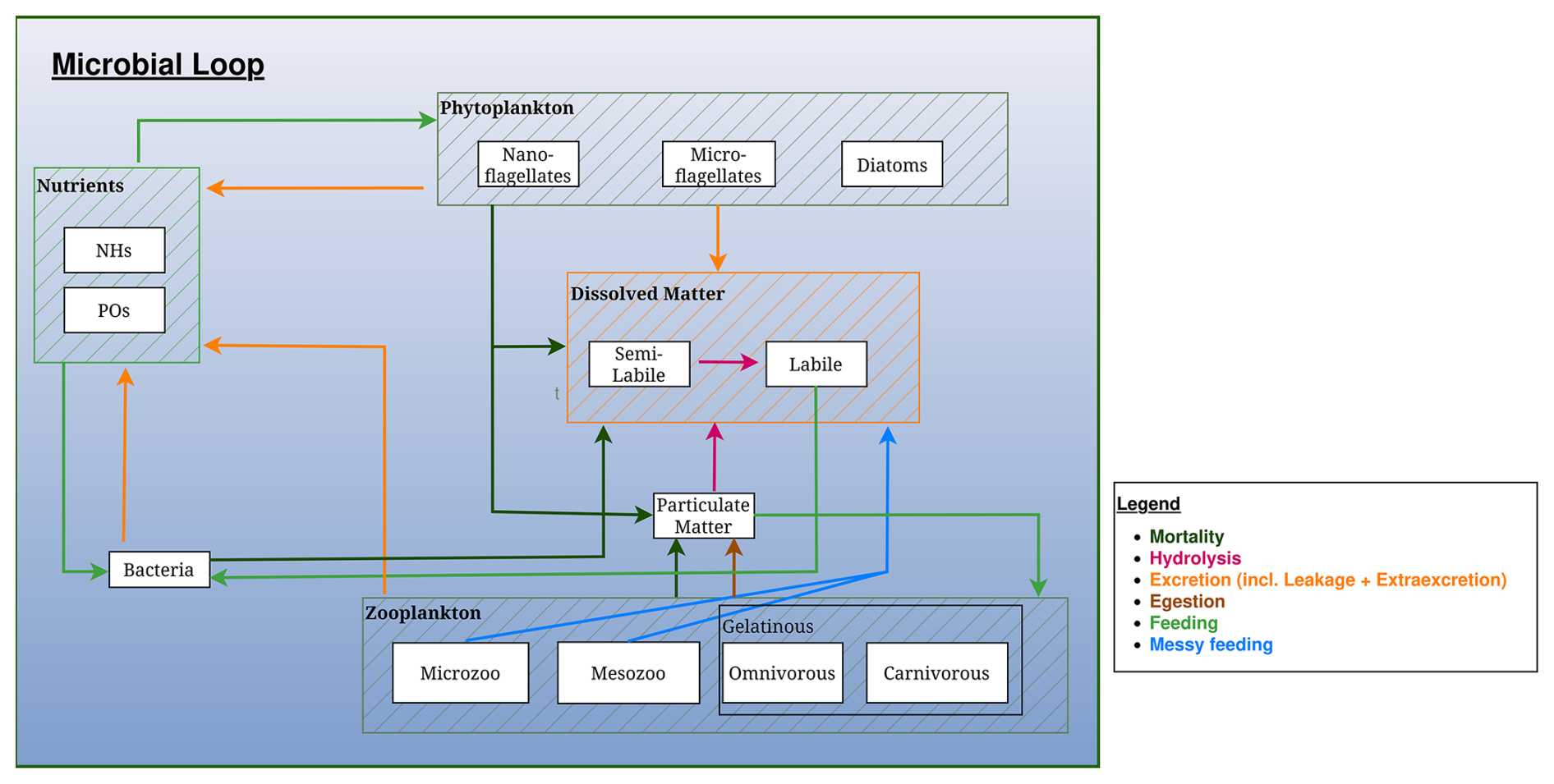
Figure 3 Schematic representation of the microbial loop in the BAMHBI biogeochemical model. The Figure shows the model state variables (in rectangular boxes) and interactions between them differentiating processes: mortality, hydrolysis, excretion, egestion, (messy) feeding and mortality. The gelatinous optional module is framed and the contribution of the gelatinous to the microbial loop is represented.

2.1.6 The dead organic pool

The dead organic matter is divided into the dissolved and particulate fractions. The dissolved pool is split into the labile (i.e., the only pool taken up directly by bacteria) and the semi-labile (i.e., the pool consisting of molecules whose eventual assimilation by the bacteria requires ectoenzyme hydrolysis to the labile pool) parts. Each dead organic pool is permitted a variable C:N ratio, giving rise to six state variables: DOCL, DONL, DOCSL, DONSL, POC and PON (see Table 1). The N:P ratio is assumed constant.

There are several sources of DOM in the model: phytoplankton excretion and lysis (Eqs. 35 and 42), zooplankton “messy feeding”, bacterial mortality (Eq. 66) and detrital breakdown (Eqs. 69 and 70). All these fluxes (except phytoplankton leakage which is assumed to produce only labile DOM) are partitioned between the labile and semi-labile pools with a single parameter δ₁ as in Anderson and Pondaven (2003). The breakdown of the semi-labile DOM by bacteria into labile DOM is described by Michaelis-Menten kinetics (Eqs. 67 and 68), with a maximum rate (parameters MaxHydDOM) and a half-saturation constant (parameter k_sat,hydDOM). The organic matter decomposition under anaerobic conditions is not as efficient as in aerobic conditions (Hedges et al., 1999). This lower efficiency is parameterized by multiplying the degradation rates by a limitation function of O₂ (Eqs. 69 and 70).

For the dead particulate organic matter we consider a preferential decomposition of N (parameter MaxHydPON) relative to C (parameter MaxHydPOC) (Anderson and Pondaven, 2003). By default, POC and PON have a constant sinking speed SinkingRatePOM_constant. If the aggregation module is activated the sinking speed of POC and PON is computed using the aggregation model described in Sect. 2.2.3

2.1.7 The inorganic pool

NOs, NHs, POs and for diatoms, SiOs, are taken up by phytoplankton according to Eqs. (39) and (40). NHs and POs are excreted by heterotrophs according to the Redfield N:P ratio. SiOs is produced by the chemical dissolution of siliceous detritus (Eq. 71).

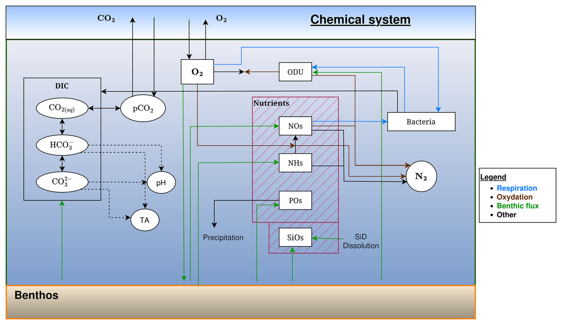
Figure 4 Schematic representation of the flows of inorganic elements in the BAMHBI biogeochemical model showing the model state variables (in rectangular boxes) and interactions between them in anaerobic conditions.

In the oxygenated part of the water column, NHs is converted into NOs through nitrification. This process is described as first-order in NHs and limited by O₂ concentration (Eq. 72). Bacterial respiration in C is computed according to Eqs. (58) and (61). The electron acceptor is successively O₂, NOs and then other oxidants (i.e., MnO₂, Fe₂O₃, SO₄) that are not explicitly modelled because they are assumed not limiting. The consumption of O₂ and NOs by bacterial respiration is limited by respectively the O₂ and NOs availability and additionally, NOs consumption is inhibited by the presence of O₂ (respectively Eqs. 62 and 63). For the modelling of anoxic degradation we follow the approach proposed by Soetaert et al. (1996) for the modelling of sediment diagenesis. We do not describe each anoxic mineralization pathway; instead they are lumped together into one process (Table A1, Eqs. A10 and A11), where degradation is only C limited (the quantity of oxidants is assumed non-limiting) and inhibited by O₂ and NOs (Table A1, Eq. 64).

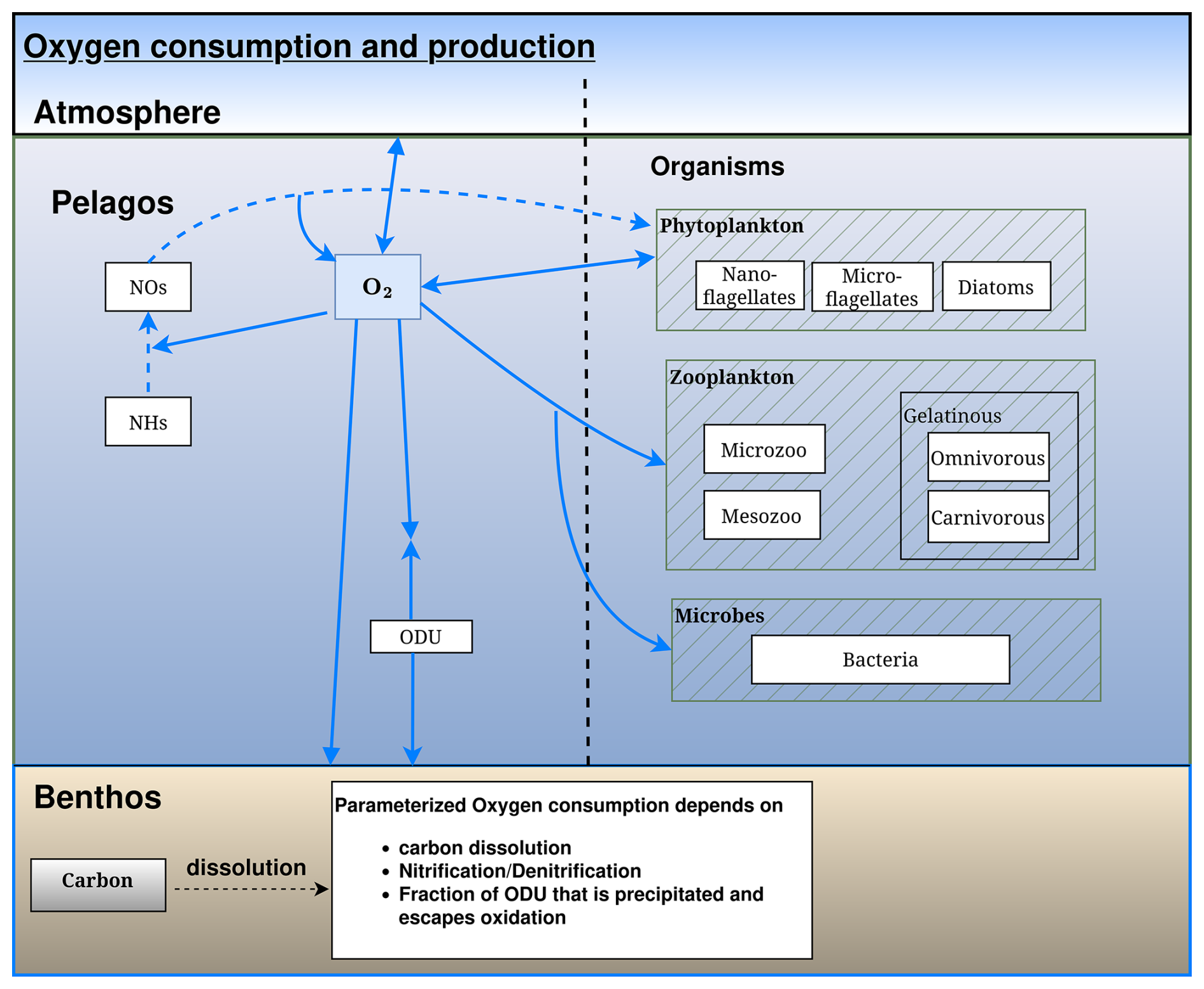
Figure 5 Schematic representation of the oxygen flows in the BAMHBI biogeochemical model showing the model state variables (in rectangular boxes) and oxygen flows between them. These oxygen flows include respiration, photosynthesis and oxidation reactions.

All the reduced substances formed by anoxic mineralisation are lumped into one state variable ODU (i.e. Oxygen Demand Unit) with $\mathrm{ODU}=\mathrm{0.5}{\mathrm{H}}_{\mathrm{2}}\mathrm{S}+\mathrm{2}{\mathrm{Mn}}^{\mathrm{2}+}+\mathrm{4}{\mathrm{Fe}}^{\mathrm{2}+}$. The terminal electron acceptors are not explicitly modeled; only the production of reduced substances is described. Anoxic mineralisation of 1 mol of C produces 1 mol of ODU and reoxidation of 1 mol of ODU requires 1 mol of O₂ (Table A1, Eqs. A10 and A11). The approach used to describe the anaerobic degradation of organic matter and the oxidation of the reduced substances produced is described in Appendix A.

The ODU and NHs are directly oxidized by O₂ and NOs. The oxidation by O₂ is limited by the availability in O₂ while the oxidation by NOs is limited by NOs and inhibited by O₂ (Eqs. 72, 73, 74 and 75). The denitrification process and the oxidation of NHs and ODU by NOs (respectively Eqs. 73 and 75) produce dinitrogen gas and constitute a loss of fixed nitrogen for the system. A part of the formed ODU is permanently removed as metal sulfides where dissolved metals are available. This process is limited by iron availability according to a Michaelis–Menten function. A dissolved iron profile needs to be imposed to the model (Eq. 65).

Temperature function

$$\begin{array}{}\text{(26)}& {\displaystyle }{f}^T=Q_{\mathrm{10}}^{\frac{T-\mathrm{20}}{\mathrm{10}}}\end{array}$$

Light penetration

$$\begin{array}{ll}\text{(27)}& {\displaystyle }& {\displaystyle }{\mathrm{PAR}}_{\mathrm{0}}=(\mathrm{1}-\text{albedo})(\mathrm{1}-p_{\mathrm{IR}})Q_{\mathrm{s},\mathrm{0}}{\displaystyle }& {\displaystyle \frac{\partial \mathrm{PAR}}{\partial z}}=-{\mathrm{PAR}}_{\mathrm{0}}\left\{\mathrm{pLong}\left(k_{\mathrm{Long}}\right)\right.\\ \text{(28)}& {\displaystyle }& {\displaystyle }\left.+\left(\mathrm{1}-\mathrm{pLong}\right)\left(k_{\mathrm{Short}}\right)\right\}{\displaystyle }& {\displaystyle }{k}_{\mathit{\lambda }}=m_{\mathrm{0}}{a}_{\mathit{\lambda }}+m_{\mathrm{1}}(\mathrm{1}-m_{\mathrm{2}}\exp \left[-m_{\mathrm{3}}{a}_{\mathit{\lambda }}\right])b_{\mathit{\lambda }}\\ \text{(29)}& {\displaystyle }& {\displaystyle }\text{for}\mathit{\lambda }=\text{Short, Long}\text{(30)}& {\displaystyle }& {\displaystyle }{m}_{\mathrm{0}}=\mathrm{1}+\mathrm{0.005}\mathit{\theta }{\displaystyle }& {\displaystyle }{a}_{\mathit{\lambda }}=a_{\mathit{\lambda },\mathrm{sw}}+a_{\mathit{\lambda },\mathrm{Chl}}^{*}{\mathrm{Chl}}^{{\widehat{a}}_{\mathit{\lambda },\mathrm{Chl}}}\\ {\displaystyle }& {\displaystyle }+[a_{\mathit{\lambda },\mathrm{CDOM}}^{*}-a_{\mathit{\lambda },\mathrm{CDOM}}^{**}\cdot \text{Salinity}]\\ \text{(31)}& {\displaystyle }& {\displaystyle }+a_{\mathit{\lambda },\mathrm{POC}}^{*}\mathrm{POC}\text{for}\mathit{\lambda }=\text{Short, Long}{\displaystyle }& {\displaystyle }{b}_{\mathit{\lambda }}=b_{\mathit{\lambda },\mathrm{sw}}+\sum _{i=\mathrm{1}}^{\mathrm{3}}\left(b_{\mathit{\lambda },{\mathrm{PHY}}_i}^{*}{\text{CPHY}}_i\right)+b_{\mathit{\lambda },\mathrm{POC}}^{*}\mathrm{POC}\\ \text{(32)}& {\displaystyle }& {\displaystyle }\text{for}\mathit{\lambda }=\text{Short, Long}\end{array}$$

Phytoplankton

Photosynthesis

$$\begin{array}{ll}{\displaystyle }& {\displaystyle }{\text{PhotosynthesisPHY}}_i=P_{max,i}{\lim }_{\mathrm{light},i}\\ {\displaystyle }& {\displaystyle }{\text{CPHY}}_i\text{for}(i=\mathrm{1},\mathrm{2},\mathrm{3})\\ \text{(33)}& {\displaystyle }& {\displaystyle }\text{with}\left\{\begin{array}{l}{\lim }_{\mathrm{light},i}=\mathrm{1}-\exp \left[\frac{-{\mathit{\alpha }}_i^{\mathrm{Chl}}\mathrm{PAR}}{{\mathit{\mu }}_{max,i}}\right]\text{for}(i=\mathrm{1},\mathrm{2},\mathrm{3})\\ P_{max,i}={\mathit{\mu }}_{max,i}{f}^T{\lim }_{\mathrm{nut},i}\text{for}(i=\mathrm{1},\mathrm{2},\mathrm{3})\\ {\lim }_{\mathrm{nut},i}=\left(\mathrm{1}-\frac{(\mathrm{N}:\mathrm{C}{)}_{{\mathrm{PHY}}_i,min}}{(\mathrm{N}:\mathrm{C}{)}_{{\mathrm{PHY}}_i}}\right)\text{for}(i=\mathrm{1},\mathrm{2},\mathrm{3})\end{array}\right.{\displaystyle }& {\displaystyle }{\text{RespirationPHY}}_i={\text{ActivityRespPHY}}_i\\ {\displaystyle }& {\displaystyle }+{\text{BasalRespPHY}}_i\\ \text{(34)}& {\displaystyle }& {\displaystyle }\text{with}\left\{\begin{array}{l}{\text{ActivityRespPHY}}_i={\text{ProdResp}}_i{\text{PhotosynthesisPHY}}_i\\ {\text{BasalRespPHY}}_i={\text{Resp}}_i{f}^T{\text{CPHY}}_i\end{array}\right.{\displaystyle }& {\displaystyle }{\text{ExcretionCPHY}}_i={\text{LeakageCPHY}}_i\\ {\displaystyle }& {\displaystyle }+{\text{ExtraExrCPHY}}_i\\ \text{(35)}& {\displaystyle }& {\displaystyle }\text{with}\left\{\begin{array}{l}{\text{LeakageCPHY}}_i={\mathit{\gamma }}_{\mathrm{1}}{\text{PhotosynthesisPHY}}_i\\ {\text{ExtraExrCPHY}}_i={\mathit{\gamma }}_{\mathrm{2}}\\ \left[{\text{PhotosynthesisPHY}}_i{|}_{(\mathrm{N}:\mathrm{C}{)}_{{\mathrm{PHY}}_i}=(\mathrm{N}:\mathrm{C}{)}_{{\mathrm{PHY}}_{i,max}}}\right.\\ \left.-{\text{PhotosynthesisPHY}}_i\right]\end{array}\right.\text{(36)}& {\displaystyle }& {\displaystyle }\text{Chlorophyll}=\sum _{i=\mathrm{1}}^{\mathrm{3}}{\text{CPHY}}_i(\mathrm{Chl}:\mathrm{C}{)}_{{\mathrm{PHY}}_i}\end{array}$$

Chl:C

$$\begin{array}{}\text{(37)}& {\displaystyle }\left\{\begin{array}{l}\text{for}(\mathrm{N}:\mathrm{C}{)}_{{\mathrm{PHY}}_i,min}\le (\mathrm{N}:\mathrm{C}{)}_{{\mathrm{PHY}}_i}\le (\mathrm{N}:\mathrm{C}{)}_{{\mathrm{PHY}}_i,max}:\\ (\mathrm{Chl}:\mathrm{C}{)}_{{\mathrm{PHY}}_i}=(\mathrm{N}:\mathrm{C}{)}_{{\mathrm{PHY}}_i}\left\{(\mathrm{Chl}:\mathrm{N}{)}_{{\mathrm{PHY}}_i,min}+\left[(\mathrm{Chl}:\mathrm{N}{)}_{{\mathrm{PHY}}_i,max}\mathrm{\dots }\right.\right.\\ \mathrm{\dots }\mathrm{..}-(\mathrm{Chl}:\mathrm{N}{)}_{{\mathrm{PHY}}_i,min}\times \frac{(\mathrm{N}:\mathrm{C}{)}_{{\mathrm{PHY}}_i}-(\mathrm{N}:\mathrm{C}{)}_{{\mathrm{PHY}}_i,min}}{(\mathrm{N}:\mathrm{C}{)}_{{\mathrm{PHY}}_i,max}-(\mathrm{N}:\mathrm{C}{)}_{{\mathrm{PHY}}_i,min}}\\ \text{for}(\mathrm{N}:\mathrm{C}{)}_{{\mathrm{PHY}}_i}\le (\mathrm{N}:\mathrm{C}{)}_{{\mathrm{PHY}}_i,min}\\ (\mathrm{Chl}:\mathrm{C}{)}_{{\mathrm{PHY}}_i}=(\mathrm{N}:\mathrm{C}{)}_{{\mathrm{PHY}}_i,min}(\mathrm{Chl}:\mathrm{N}{)}_{{\mathrm{PHY}}_i,min}\\ \text{for}\mathrm{N}:\mathrm{C}{)}_{{\mathrm{PHY}}_i}\ge (\mathrm{N}:\mathrm{C}{)}_{{\mathrm{PHY}}_i,max}\\ (\mathrm{Chl}:\mathrm{C}{)}_{{\mathrm{PHY}}_i}=(\mathrm{N}:\mathrm{C}{)}_{{\mathrm{PHY}}_i,max}(\mathrm{Chl}:\mathrm{N}{)}_{{\mathrm{PHY}}_i,max}\end{array}\right.\end{array}$$

Nutrient Uptake

${\mathrm{NOs}}_i^{\mathrm{uptake}},{\mathrm{NHs}}_i^{\mathrm{uptake}},{\text{POs}}_i^{\mathrm{uptake}},{\mathrm{SiOs}}_{\mathrm{3}}^{\mathrm{uptake}}$ for (Nut:C)${}_{{\mathrm{PHY}}_i}\le (\mathrm{Nut}:\mathrm{C}{)}_{{\mathrm{PHY}}_{i,max}}$ with Nut $=\mathrm{N},\mathrm{P},\mathrm{Si}$ (for diatoms).

$$\begin{array}{}\text{(38)}& {\displaystyle }& {\displaystyle }\left\{\begin{array}{l}{\mathrm{NOs}}_i^{\mathrm{uptake}}{|}_{\mathrm{potential}}={\mathrm{NOumax}}_i{f}^T\\ \left(\mathrm{1}-\frac{(\mathrm{N}:\mathrm{C}{)}_{{\mathrm{PHY}}_i}}{(\mathrm{N}:\mathrm{C}{)}_{{\mathrm{PHY}}_{i,max}}}\right)\frac{\mathrm{NOs}}{\mathrm{NOs}+k_{{\mathrm{NOs}}_i}}\frac{k_{in}}{k_{in}+\mathrm{NHs}}{\text{CPHY}}_i\\ {\mathrm{NHs}}_i^{\mathrm{uptake}}{|}_{\mathrm{potential}}={\mathrm{NHumax}}_i{f}^T\\ \left(\mathrm{1}-\frac{(\mathrm{N}:\mathrm{C}{)}_{{\mathrm{PHY}}_{\mathrm{3}}}}{(\mathrm{N}:\mathrm{C}{)}_{{\mathrm{PHY}}_{i,max}}}\right)\frac{\mathrm{NHs}}{\mathrm{NHs}+k_{{\mathrm{NHs}}_i}}{\text{CPHY}}_i\\ {\mathrm{PO}}_s^{\mathrm{uptake}}{|}_{\mathrm{potential}}={\mathrm{Pumax}}_i{f}^T\\ \left(\mathrm{1}-\frac{(P:C{)}_{{\mathrm{PHY}}_i}}{(\mathrm{P}:\mathrm{C}{)}_{{\mathrm{PHY}}_{i,max}}}\right)\frac{\mathrm{POs}}{\mathrm{POs}+k_{{\mathrm{POs}}_i}}{\text{CPHY}}_i\\ {\mathrm{SiOs}}_{\mathrm{3}}^{\mathrm{uptake}}{|}_{\mathrm{potential}}=\mathrm{Si}\mathrm{umax}{f}^T\\ \left(\mathrm{1}-\frac{(\mathrm{Si}:\mathrm{C}{)}_{{\mathrm{PHY}}_{\mathrm{3}}}}{(\mathrm{Si}:\mathrm{C}{)}_{{\mathrm{PHY}}_{\mathrm{3},max}}}\right)\frac{\mathrm{SiOs}}{\mathrm{SiOs}+k_{{\mathrm{SiOs}}_{\mathrm{3}}}}{\text{CPHY}}_{\mathrm{3}}\\ \text{for diatoms}i=\mathrm{3}\end{array}\right.\text{(39)}& {\displaystyle }& {\displaystyle }\left\{\begin{array}{l}{\mathrm{Nitrogen}}_{{\mathrm{PHY}}_i}^{\mathrm{uptake}}=min\\ \left({\mathrm{NOs}}_i^{\mathrm{uptake}}{|}_{\mathrm{potential}}+{\mathrm{NHs}}_i^{\mathrm{uptake}}{|}_{\mathrm{potential}},\right.\\ \left.\frac{{\mathrm{PO}}_s^{\mathrm{uptake}}{|}_{\mathrm{potential}}}{(\mathrm{P}:\mathrm{N}{)}_{{\mathrm{PHY}}_i}},{\mathit{\delta }}_{i,\mathrm{3}}\frac{{\mathrm{SiOs}}_{\mathrm{3}}^{\mathrm{uptake}}{|}_{\mathrm{potential}}}{(\mathrm{Si}:\mathrm{N}{)}_{{\mathrm{PHY}}_{\mathrm{3}}}}\right)\\ {\mathrm{NOs}}_i^{\mathrm{uptake}}=\frac{{\mathrm{Nitrogen}}_{{\mathrm{PHY}}_i}^{\mathrm{uptake}}}{{\mathrm{NOs}}_i^{\mathrm{uptake}}{|}_{\mathrm{potential}}+{\mathrm{NHs}}_i^{\mathrm{uptake}}{|}_{\mathrm{potential}}}\\ {\mathrm{NOs}}_i^{\mathrm{uptake}}{|}_{\mathrm{potential}}\\ {\mathrm{NHs}}_i^{\mathrm{uptake}}=\frac{{\mathrm{Nitrogen}}_{{\mathrm{PHY}}_i}^{\mathrm{uptake}}}{{\mathrm{NOs}}_i^{\mathrm{uptake}}{|}_{\mathrm{potential}}+{\mathrm{NHs}}_i^{\mathrm{uptake}}{|}_{\mathrm{potential}}}\\ {\mathrm{NHs}}_i^{\mathrm{uptake}}{|}_{\mathrm{potential}}\\ {\mathrm{POs}}_i^{\mathrm{uptake}}=\frac{{\mathrm{Nitrogen}}_{{\mathrm{PHY}}_i}^{\mathrm{uptake}}}{(\mathrm{P}:\mathrm{N}{)}_{{\mathrm{PHY}}_i}}\\ {\mathrm{SiOs}}_{\mathrm{3}}^{\mathrm{uptake}}=\left[\frac{{\mathrm{Nitrogen}}_{{\mathrm{PHY}}_{\mathrm{3}}}^{\mathrm{uptake}}}{(\mathrm{Si}:\mathrm{N}{)}_{{\mathrm{PHY}}_{\mathrm{3}}}}-{\mathrm{LeakageNPHY}}_{\mathrm{3}}\right]\\ (\mathrm{Si}:\mathrm{N}{)}_{{\mathrm{PHY}}_{\mathrm{3}}}\end{array}\right.\end{array}$$

Excretion

for $(\mathrm{Nut}:\mathrm{C}{)}_{{\mathrm{PHY}}_i}\ge (\mathrm{Nut}:\mathrm{C}{)}_{{\mathrm{PHY}}_i,max}$ with Nut = N, P, Si (for diatoms). We have a negative uptake that corresponds to an excretion.

$$\begin{array}{}\text{(40)}& {\displaystyle }\left\{\begin{array}{l}{\mathrm{NOs}}_i^{\mathrm{uptake}}=\mathrm{0}\\ {\mathrm{NH}}_{s,\mathrm{3}}^{\mathrm{uptake}}{|}_{\mathrm{potential}}={\mathrm{NHumax}}_i{f}^T\\ \left(\mathrm{1}-\frac{(\mathrm{N}:\mathrm{C}{)}_{{\mathrm{PHY}}_i}}{(\mathrm{N}:\mathrm{C}{)}_{{\mathrm{PHY}}_{i,max}}}\right){\text{CPHY}}_i\\ {\mathrm{POs}}_i^{\mathrm{uptake}}{|}_{\mathrm{potential}}={\mathrm{Pumax}}_i{f}^T\\ \left(\mathrm{1}-\frac{(\mathrm{P}:\mathrm{C}{)}_{{\mathrm{PHY}}_i}}{(\mathrm{P}:\mathrm{C}{)}_{{\mathrm{PHY}}_{i,max}}}\right){\text{CPHY}}_i\\ {\mathrm{SiOs}}_{\mathrm{3}}^{\mathrm{uptake}}{|}_{\mathrm{potential}}=\mathrm{SiOsumax}{f}^T\\ \left(\mathrm{1}-\frac{(\mathrm{Si}:\mathrm{C}{)}_{{\mathrm{PHY}}_{\mathrm{3}}}}{(\mathrm{Si}:\mathrm{C}{)}_{{\mathrm{PHY}}_{\mathrm{3},max}}}\right){\text{CPHY}}_{\mathrm{3}}\\ {\mathrm{NHs}}_i^{\mathrm{uptake}}=min\left({\mathrm{NHs}}_i^{\mathrm{uptake}}{|}_{\mathrm{potential}},\frac{{\mathrm{POs}}_i^{\mathrm{uptake}}{|}_{\mathrm{potential}}}{(\mathrm{P}:\mathrm{N}{)}_{{\mathrm{PHY}}_i}},\right.\\ \left.{\mathit{\delta }}_{i,\mathrm{3}}\frac{{\mathrm{SiOs}}_{\mathrm{3}}^{\mathrm{uptake}}{|}_{\mathrm{potential}}}{(\mathrm{Si}:\mathrm{N}{)}_{{\mathrm{PHY}}_{\mathrm{3}}}}\right)\\ {\mathrm{POs}}_i^{\mathrm{uptake}}=\frac{{\mathrm{NHs}}_i^{\mathrm{uptake}}}{(\mathrm{P}:\mathrm{N}{)}_{{\mathrm{PHY}}_i}},{\mathrm{SiOs}}_{\mathrm{3}}^{\mathrm{uptake}}=\frac{{\mathrm{NHs}}_i^{\mathrm{uptake}}}{(\mathrm{Si}:\mathrm{N}{)}_{{\mathrm{PHY}}_{\mathrm{3}}}}\end{array}\right.\end{array}$$

Leakage

$$\begin{array}{}\text{(41)}& {\displaystyle }\left\{\begin{array}{l}{\mathrm{LeakageNPHY}}_i={\mathit{\gamma }}_{\mathrm{1}}\left({\mathrm{NH}}_{s,\mathrm{1}}^{\mathrm{uptake}}+{\mathrm{NO}}_{s,\mathrm{1}}^{\mathrm{uptake}}\right)\\ {\mathrm{LeakageNPHY}}_i=\mathrm{0}\text{when}(\mathrm{N}:\mathrm{C}{)}_{{\mathrm{PHY}}_i}>(\mathrm{N}:\mathrm{C}{)}_{{\mathrm{PHY}}_{i,max}}\end{array}\right.\end{array}$$

Mortality

$$\begin{array}{}\text{(42)}& {\displaystyle }{\text{MortPHY}}_{X,i}={\mathrm{mort}}_{{\mathrm{PHY}}_i}{f}^T{\text{XPHY}}_i,X=\mathrm{C},\mathrm{N},\mathrm{Chl}\end{array}$$

Sedimentation of Diatoms

$$\begin{array}{ll}{\displaystyle }& {\displaystyle }{v}_{{\mathrm{Phy}}_{\mathrm{3}}}=v_{{\mathrm{Phy}}_{\mathrm{3},min}}+\left(v_{{\mathrm{Phy}}_{\mathrm{3},max}}-v_{{\mathrm{Phy}}_{\mathrm{3},min}}\right)\\ \text{(43)}& {\displaystyle }& {\displaystyle }{\displaystyle \frac{\left((\mathrm{N}:\mathrm{C}{)}_{{\mathrm{PHY}}_{\mathrm{3},max}}-(\mathrm{N}:\mathrm{C}{)}_{{\mathrm{PHY}}_{\mathrm{3}}}\right)}{\left((\mathrm{N}:\mathrm{C}{)}_{{\mathrm{PHY}}_{\mathrm{3},max}}-(\mathrm{N}:\mathrm{C}{)}_{{\mathrm{PHY}}_{\mathrm{3},min}}\right)}}\end{array}$$

Zooplankton

Feeding ($i=\mathrm{1},\mathrm{2}$)

$$\begin{array}{ll}{\displaystyle }& {\displaystyle }{\text{GrazZOO}}_{\mathrm{C},i}=f^T{\text{MaxGrazZOO}}_i\\ \text{(44)}& {\displaystyle }& {\displaystyle }{\displaystyle \frac{{\mathrm{Ba}}_{\mathrm{C},{\mathrm{ZOO}}_i}}{{\mathrm{Ba}}_{\mathrm{C},{\mathrm{ZOO}}_i}+k_{\mathrm{sat},{\mathrm{ZOO}}_i}}}{\text{CZOO}}_i\text{(45)}& {\displaystyle }& {\displaystyle }{\text{GrazZOO}}_{\mathrm{N},i}={\text{GrazZOO}}_{\mathrm{C},i}(\mathrm{N}:\mathrm{C}{)}_{\mathrm{food},i}\text{(46)}& {\displaystyle }& {\displaystyle }{\mathrm{Ba}}_{X,{\mathrm{ZOO}}_i}=\sum _{\mathrm{preys}}{e}_{\mathrm{Prey},{\mathrm{ZOO}}_i}\mathrm{XPrey}X=\mathrm{C},\mathrm{N}\text{(47)}& {\displaystyle }& {\displaystyle }(\mathrm{N}:\mathrm{C}{)}_{\mathrm{food},i}={\mathrm{Ba}}_{{\mathrm{N},\mathrm{ZOO}}_i}/{\mathrm{Ba}}_{\mathrm{C},{\mathrm{ZOO}}_i}\text{(48)}& {\displaystyle }& {\displaystyle }{I}_{X,i}=(\mathrm{1}-{\mathit{\varphi }}_i){\text{GrazZOO}}_{X,i}X=\mathrm{C},\mathrm{N}{\displaystyle }& {\displaystyle }{\text{Graz}}_{\mathrm{Prey}}=\sum _{i=\mathrm{1}}^{\mathrm{2}}\left[{\displaystyle \frac{{\text{GrazZOO}}_{\mathrm{C},i}}{{\mathrm{Ba}}_{\mathrm{C},{\mathrm{ZOO}}_i}}}{e}_{\mathrm{Prey},{\mathrm{ZOO}}_i}\mathrm{Prey}\right]\\ {\displaystyle }& {\displaystyle }\text{Prey}={\text{CPHY}}_i,{\text{NPHY}}_i,{\mathrm{ChlPHY}}_i,\text{CBAC, POC},\\ \text{(49)}& {\displaystyle }& {\displaystyle }\text{PON},{\text{CZOO}}_{\mathrm{1}}\end{array}$$

Growth, ($i=\mathrm{1},\mathrm{2}$)

$$\begin{array}{ll}{\displaystyle }& {\displaystyle }(\mathrm{N}:\mathrm{C}{)}_i^{*}=(\mathrm{N}:\mathrm{C}{)}_{{\mathrm{ZOO}}_i}{\displaystyle \frac{k_{c,i}{\mathit{\beta }}_{\mathrm{C},i}}{{\mathit{\beta }}_{\mathrm{N},i}}}\to \\ \text{(50)}& {\displaystyle }& {\displaystyle }\left\{\begin{array}{l}(\mathrm{N}:\mathrm{C}{)}_{\mathrm{food},i}<(\mathrm{N}:\mathrm{C}{)}_i^{*}\Rightarrow \text{N limitation}\\ (\mathrm{N}:\mathrm{C}{)}_{\mathrm{food},i}>(\mathrm{N}:\mathrm{C}{)}_i^{*}\Rightarrow \text{C limitation}\end{array}\right.{\displaystyle }& {\displaystyle }\text{If N limits:}\\ \text{(51)}& {\displaystyle }& {\displaystyle }\left\{\begin{array}{l}{\text{GrowthZOO}}_{\mathrm{N},i}={\mathit{\beta }}_{\mathrm{N},i}{I}_{\mathrm{N},i}\\ {\text{GrowthZOO}}_{\mathrm{C},i}={\text{GrowthZOO}}_{\mathrm{N},i}/(\mathrm{N}:\mathrm{C}{)}_{\mathrm{ZOO}}\\ {\text{ExcrZOO}}_i=\mathrm{0}\end{array}\right.{\displaystyle }& {\displaystyle }\text{If C limits:}\\ \text{(52)}& {\displaystyle }& {\displaystyle }\left\{\begin{array}{l}{\text{GrowthZOO}}_{\mathrm{C},i}=k_{c,i}{\mathit{\beta }}_{\mathrm{C},i}{I}_{\mathrm{C},i}\\ {\text{GrowthZOO}}_{\mathrm{N},i}={\text{GrowthZOO}}_{\mathrm{C},i}(\mathrm{N}:\mathrm{C}{)}_{{\mathrm{ZOO}}_j}\\ {\text{ExcrZOO}}_i={\mathit{\beta }}_{\mathrm{N},i}{I}_{\mathrm{N},i}-{\text{GrowthZOO}}_{\mathrm{N},i}\end{array}\right.\text{(53)}& {\displaystyle }& {\displaystyle }{\text{RespZOO}}_i={\mathit{\beta }}_{\mathrm{C},i}{I}_{\mathrm{C},i}-{\text{GrowthZOO}}_{\mathrm{C},i}\end{array}$$

Mortality, ($i=\mathrm{1},\mathrm{2}$)

$$\begin{array}{ll}{\displaystyle }& {\displaystyle }{\text{MortZOO}}_{\mathrm{C},i}\\ {\displaystyle }& {\displaystyle }=f^{\mathrm{T}}\left({\mathrm{CZOO}}_i^{\mathrm{2}}{\mathrm{mortZOO}}_i{\displaystyle \frac{{\mathrm{CZOO}}_i}{{\mathrm{CZOO}}_i+{\mathrm{ksat}}_{{\mathrm{MortZOO}}_i}}}\right.\\ \text{(54)}& {\displaystyle }& {\displaystyle }\left.+{\mathrm{CZOO}}_i\left(\mathrm{1}-{\displaystyle \frac{{\mathrm{O}}_{\mathrm{2}}}{{\mathrm{O}}_{\mathrm{2}}+{\mathrm{ksat}}_{\mathrm{AnoxMort}}}}\right)\mathrm{AnoxMort}\right)\end{array}$$

Microbial Loop

Bacteria Growth, respiration, excretion and mortality

$$\begin{array}{ll}{\displaystyle }& {\displaystyle }{U}_c=f^T{\mathit{\mu }}_{\mathrm{BAC}}{\displaystyle \frac{\mathrm{DOCL}}{k_{\mathrm{BAC},\mathrm{DOC}}+\mathrm{DOCL}}}\text{CBAC},\\ \text{(55)}& {\displaystyle }& {\displaystyle }{U}_n=U_c\left({\displaystyle \frac{\mathrm{DONL}}{\mathrm{DOCL}}}\right)\text{(56)}& {\displaystyle }& {\displaystyle }{U}_A^{*}=f^T{\mathit{\mu }}_{\mathrm{BAC}}{\displaystyle \frac{\mathrm{NHs}}{k_{\mathrm{BAC},\mathrm{NHs}}+\mathrm{NHs}}}\text{CBAC}(\mathrm{N}:\mathrm{C}{)}_{\mathrm{BAC}}\text{(57)}& {\displaystyle }& {\displaystyle }\text{TestBAC}=U_n-{\mathit{\omega }}_B{U}_c(\mathrm{N}:\mathrm{C}{)}_{\mathrm{BAC}}{\displaystyle }& {\displaystyle }\text{if}{U}_A^{*}>-\text{TestBAC}\to \text{Carbon limitation case:}\\ {\displaystyle }& {\displaystyle }\text{GrowthBAC}={\mathit{\omega }}_B{U}_c\\ \text{(58)}& {\displaystyle }& {\displaystyle }\text{RespBAC}=(\mathrm{1}-{\mathit{\omega }}_B)U_c{\displaystyle }& {\displaystyle }\text{if TestBAC}<\mathrm{0}\to \text{NHs uptake is necessary}\\ {\displaystyle }& {\displaystyle }\text{to consume all the DOCL}\\ {\displaystyle }& {\displaystyle }{U}_{\mathrm{A}}=-\text{TestBAC}\\ \text{(59)}& {\displaystyle }& {\displaystyle }\text{ExcrBAC}=\mathrm{0}{\displaystyle }& {\displaystyle }\text{if TestBAC}>\mathrm{0}\to \text{Bacteria act as remineralizers:}\\ {\displaystyle }& {\displaystyle }{U}_{\mathrm{A}}=\mathrm{0}\\ \text{(60)}& {\displaystyle }& {\displaystyle }\text{ExcrBAC}=\text{TestBAC}{\displaystyle }& {\displaystyle }\text{if}{U}_A^{*}\le -\text{TestBAC}\to \text{Nitrogen Limitation case:}\\ \text{(61)}& {\displaystyle }& {\displaystyle }\begin{array}{l}{U}_{\mathrm{A}}=U_{\mathrm{A}}^{*}\\ \text{GrowthBAC}=(U_n+U_{\mathrm{A}})/(\mathrm{N}:\mathrm{C}{)}_{\mathrm{BAC}}\\ \text{RespBAC}=\text{GrowthBAC}\left(\mathrm{1}/{\mathit{\omega }}_B-\mathrm{1}\right)\\ \text{ExcrBAC}=\mathrm{0}\end{array}\text{(62)}& {\displaystyle }& {\displaystyle }\text{RespBACOxygen}=\text{RespBAC}{\displaystyle \frac{{\mathrm{O}}_{\mathrm{2}}}{{\mathrm{O}}_{\mathrm{2}}+k_{\mathrm{sat},{\mathrm{O}}_{\mathrm{2}}}^{\text{OxicMin}}}}{\displaystyle }& {\displaystyle }\text{RespBACNitrate}=\text{RespBAC}{\displaystyle \frac{\mathrm{NOs}}{\mathrm{NOs}+k_{\mathrm{sat},\mathrm{NOs}}^{\mathrm{Denit}}}}\\ \text{(63)}& {\displaystyle }& {\displaystyle }\left(\mathrm{1}-{\displaystyle \frac{{\mathrm{O}}_{\mathrm{2}}}{{\mathrm{O}}_{\mathrm{2}}+k_{\mathrm{in},{\mathrm{O}}_{\mathrm{2}}}^{\mathrm{Denit}}}}\right){\displaystyle }& {\displaystyle }\text{AnoxicRespBAC}=\text{RespBAC}\left(\mathrm{1}-{\displaystyle \frac{\text{NOs}}{\text{NOs}+k_{\mathrm{in},\mathrm{NOs}}^{\mathrm{AnoxMin}}}}\right)\\ \text{(64)}& {\displaystyle }& {\displaystyle }\left(\mathrm{1}-{\displaystyle \frac{{\mathrm{O}}_{\mathrm{2}}}{{\mathrm{O}}_{\mathrm{2}}+k_{\mathrm{in},{\mathrm{O}}_{\mathrm{2}}}^{\mathrm{AnoxMin}}}}\right){\displaystyle }& {\displaystyle }\text{SolidODU}=R_{\mathrm{solid}}\text{IronLimitation}{\mathit{\gamma }}_{\mathrm{POC}}^{\mathrm{ODU}}\text{AnoxicRespBAC}\\ {\displaystyle }& {\displaystyle }\text{with IronLimitation}={\displaystyle \frac{\mathrm{Iron}}{\mathrm{Iron}+k_{\mathrm{sat},\mathrm{iron}}^{\mathrm{SolForm}}}}\\ \text{(65)}& {\displaystyle }& {\displaystyle }\text{where Iron concentration is taken from the data}\text{(66)}& {\displaystyle }& {\displaystyle }\text{MortBAC}=f^T{\mathrm{mort}}_{\mathrm{BAC}}\text{CBAC}\end{array}$$

Labile and Semi-labile Dissolved Organic Matter

$$\begin{array}{ll}{\displaystyle }& {\displaystyle }\mathrm{HydrolDOCSL}=f^T\mathrm{MaxHydDOM}\\ \text{(67)}& {\displaystyle }& {\displaystyle }{\displaystyle \frac{\mathrm{DOCSL}}{\mathrm{DOCSL}+k_{\mathrm{sat},\mathrm{hydDOM}}}}\mathrm{CBAC}\text{(68)}& {\displaystyle }& {\displaystyle }\mathrm{HydrolDONSL}=\mathrm{HydrolDOCSL}{\displaystyle \frac{\mathrm{DONSL}}{\mathrm{DOCSL}}}\end{array}$$

Particulate Detritial Matter

$$\begin{array}{ll}{\displaystyle }& {\displaystyle }\mathrm{HydrolPOC}=f^T\mathrm{MaxHydPOC}\\ \text{(69)}& {\displaystyle }& {\displaystyle }{\displaystyle \frac{{\mathrm{O}}_{\mathrm{2}}+\mathrm{1}}{{\mathrm{O}}_{\mathrm{2}}+\mathrm{1}+k_{\mathrm{sat},\mathrm{OxicHydrol}}}}\mathrm{POC}{\displaystyle }& {\displaystyle }\mathrm{HydrolPON}=f^T\mathrm{MaxHydPON}\\ \text{(70)}& {\displaystyle }& {\displaystyle }{\displaystyle \frac{{\mathrm{O}}_{\mathrm{2}}+\mathrm{1}}{{\mathrm{O}}_{\mathrm{2}}+\mathrm{1}+k_{\mathrm{sat},\mathrm{OxicHydrol}}}}\mathrm{PON}\text{(71)}& {\displaystyle }& {\displaystyle }\mathrm{DissolutionSidet}=f^T{\mathrm{diss}}_{\mathrm{SiDet}}\mathrm{SiDet}\end{array}$$

Chemical submodel

$$\begin{array}{ll}\text{(72)}& {\displaystyle }& {\displaystyle }\text{NHs}{\mathrm{oxid}}_{{\mathrm{O}}_{\mathrm{2}}}=f^T{\mathit{\mu }}_{\mathrm{NHs}}^{{\mathrm{O}}_{\mathrm{2}}}{\displaystyle \frac{{\mathrm{O}}_{\mathrm{2}}}{{\mathrm{O}}_{\mathrm{2}}+k_{\mathrm{sat},{\mathrm{O}}_{\mathrm{2}}}^{\text{NHs}\mathrm{oxid}}}}{\displaystyle }& {\displaystyle }\text{NHs}{\mathrm{oxid}}_{\mathrm{NOs}}=f^T{\mathit{\mu }}_{\mathrm{NHs}}^{\mathrm{NOs}}\\ \text{(73)}& {\displaystyle }& {\displaystyle }{\displaystyle \frac{\mathrm{NOs}}{\mathrm{NOs}+k_{\mathrm{sat},\mathrm{NOs}}^{\text{NHs}{\mathrm{oxid}}_{\mathrm{NOs}}}}}\left(\mathrm{1}-{\displaystyle \frac{{\mathrm{O}}_{\mathrm{2}}}{{\mathrm{O}}_{\mathrm{2}}+k_{\mathrm{in},{\mathrm{O}}_{\mathrm{2}}}^{\text{NHs}{\mathrm{oxid}}_{\mathrm{NOS}}}}}\right)\text{(74)}& {\displaystyle }& {\displaystyle }{\text{ODUoxid}}_{{\mathrm{O}}_{\mathrm{2}}}=f^T{\mathit{\mu }}_{\mathrm{ODU}}^{{\mathrm{O}}_{\mathrm{2}}}{\displaystyle \frac{{\mathrm{O}}_{\mathrm{2}}}{{\mathrm{O}}_{\mathrm{2}}+k_{\mathrm{sat},{\mathrm{O}}_{\mathrm{2}}}^{\mathrm{ODUoxid}}}}{\displaystyle }& {\displaystyle }{\text{ODUoxid}}_{\mathrm{NOS}}=f^T{\mathit{\mu }}_{\mathrm{ODU}}^{\mathrm{NOs}}\\ \text{(75)}& {\displaystyle }& {\displaystyle }{\displaystyle \frac{\mathrm{NOs}}{\mathrm{NOs}+k_{\mathrm{sat},\mathrm{NOs}}^{{\text{ODUoxid}}_{\mathrm{NOs}}}}}\left(\mathrm{1}-{\displaystyle \frac{{\mathrm{O}}_{\mathrm{2}}}{{\mathrm{O}}_{\mathrm{2}}+k_{\mathrm{in},{\mathrm{O}}_{\mathrm{2}}}^{{\text{ODUoxid}}_{\mathrm{NOS}}}}}\right)\end{array}$$

2.2 BAMHBI Modules

BAMHBI includes five optional modules that are summarized in Table 8 and described here below. The inclusion of such modules is explained in this section.

2.2.1 The chlorophyll module

If the chlorophyll module is activated, the Chl a content of each phytoplankton group is dynamically computed using the formulation of Geider et al. (1998). Each phytoplankton group is then described by three state variables representing their N, C and Chl a content. The dynamics of each phytoplankton group mechanistically represents the physiological acclimation process at cellular level that takes place in algae and consists in changing the cellular biochemical composition Chl a:C and C:N of algae as a function of external environmental variables: light, inorganic nutrients and temperature. The synthesis of Chl a is downregulated in conditions of inorganic nutrients limitations and is enhanced when light is limiting.

Chlorophyll

$$\begin{array}{l}\text{(76)}& {\displaystyle }& {\displaystyle }{\lim }_{\mathrm{light},i}=\mathrm{1}-\exp \left({\displaystyle \frac{-{\mathit{\alpha }}_i^{\mathrm{Chl}}(\mathrm{Chl}:\mathrm{C}{)}_{{\mathrm{PHY}}_i}\mathrm{PAR}}{{\mathit{\mu }}_{\text{max},i}}}\right)\text{(77)}& {\displaystyle }& {\displaystyle }(\mathrm{Chl}:\mathrm{C}{)}_{\text{max}}=(\mathrm{Chl}:\mathrm{N}{)}_{\text{max}}(\mathrm{N}:\mathrm{C}{)}_{\text{max}}\text{(78)}& {\displaystyle }& {\displaystyle }(\mathrm{Chl}:\mathrm{C}{)}_{\text{min}}=(\mathrm{Chl}:\mathrm{N}{)}_{\text{min}}(\mathrm{N}:\mathrm{C}{)}_{\text{min}}\text{(79)}& {\displaystyle }& {\displaystyle }{\text{SynthesisChlPHY}}_i={\displaystyle \frac{{\mathit{\rho }}_{\mathrm{Chl},i}{V}_{\mathrm{N},i}}{(\mathrm{Chl}:\mathrm{C}{)}_{{\mathrm{PHY}}_i}}}{\mathrm{ChlPHY}}_i\text{(80)}& {\displaystyle }& {\displaystyle }\text{If Nitrogen Uptake}>\mathrm{0}\to {\text{V}}_{\mathrm{N},i}={\displaystyle \frac{{\mathrm{Nitrogen}}_{{\mathrm{PHY}}_i}^{\mathrm{uptake}}}{{\text{CPHY}}_i}}\text{(81)}& {\displaystyle }& {\displaystyle }\text{If Nitrogen Uptake}<\mathrm{0}\to {\text{V}}_{\mathrm{N},i}=\mathrm{0}\text{(82)}& {\displaystyle }& {\displaystyle }\text{If PAR > 0}\to {\mathit{\rho }}_{\mathrm{Chl},i}={\displaystyle \frac{P_{max,i}{\lim }_{\mathrm{light},i}(\mathrm{Chl}:\mathrm{N}{)}_{max}}{{\mathit{\alpha }}_i^{\mathrm{Chl}}(\mathrm{Chl}:\mathrm{C}{)}_{{\mathrm{PHY}}_i}\mathrm{PAR}}}\text{(83)}& {\displaystyle }& {\displaystyle }\text{If PAR}=\mathrm{0}\to {\mathit{\rho }}_{\mathrm{Chl},i}=\mathrm{0}\text{(84)}& {\displaystyle }& {\displaystyle }{\mathrm{RespirationChlPHY}}_i={\text{Resp}}_i{f}^T{\mathrm{ChlPHY}}_i\text{(85)}& {\displaystyle }& {\displaystyle }\text{Chlorophyll}=\sum _{i=\mathrm{1}}^{\mathrm{3}}{\mathrm{ChlPHY}}_i{\displaystyle }\end{array}$$

Equations above describe the Geider module. The two mains differences with the other equation are

1. the chlorophyll content of each phytoplankton group are modelled as state variables,

2. the photosynthesis – light curve depends now on the (Chl:C) ratio as shown by Eq. (76).

In addition to these major changes, the (Chl:C) ratio is bounded between a minimal and maximal ratios computed by Eqs. (78) and (77). These bounds, also used in Aumont et al. (2015) and Butenschön et al. (2016), prevent the regulation term Eqs. (82) and (79) from being to large or too small. The nitrogen to carbon ratio used for computing the carbon uptake Eq. (33) is bounded while it is not in the computation of nutrients uptake in Eq. (38). For diatoms, the (Si:C) computation based on the (N:C) ratio and the Redfield ratio do not use the bounded (N:C) ratio.

2.2.2 The gelatinous zooplankton module

When the gelatinous module is included, a carnivorous and an omnivorous group are added to the model. Both gelatinous groups are “top-predators” and there is no trophic link between them. They have a grazing rate that linearly increases with prey concentrations without saturation and with no feeding when the food concentration is below a given threshold. The omnivorous gelatinous feeds on the three PFTs, micro- and mesozooplankton and detritus while the carnivorous gelatinous can only feed on mesozooplankton. The internal composition of gelatinous organisms is held constant by adjusting the excretion and respiration terms (set of Eqs. (94), (95) and (96)). They are not consumed and represent trophic dead-ends. The mortality terms of the two gelatinous groups are represented by the sum of a first-order kinetics as in Lancelot et al. (2002) and an additional term traducing the rapid mortality of these organisms in anoxic conditions (Eq. 97).

Gelatinous, (j= 1, 2)

$$\begin{array}{ll}\text{(86)}& {\displaystyle }& {\displaystyle }{\mathrm{GrazGEL}}_{\mathrm{C},j}=f^T{\mathrm{MaxGrazGEL}}_j{\mathrm{Ba}}_{c,{\mathrm{GEL}}_j}{\mathrm{CGEL}}_j\text{(87)}& {\displaystyle }& {\displaystyle }{\mathrm{GrazGEL}}_{\mathrm{N},j}={\mathrm{GrazGEL}}_{\mathrm{C},j}(\mathrm{N}:\mathrm{C}{)}_{\mathrm{food},j}\text{(88)}& {\displaystyle }& {\displaystyle }{\mathrm{Ba}}_{x,{\mathrm{GEL}}_j}=\sum _{\mathrm{preys}}{e}_{\mathrm{Prey},{\mathrm{GEL}}_j}\mathrm{XPrey},X=\mathrm{C},\mathrm{N}\text{(89)}& {\displaystyle }& {\displaystyle }(\mathrm{N}:\mathrm{C}{)}_{\mathrm{food},{\mathrm{GEL}}_j}={\mathrm{Ba}}_{n,{\mathrm{GEL}}_j}/{\mathrm{Ba}}_{c,{\mathrm{GEL}}_j}{\displaystyle }& {\displaystyle }{\mathrm{GrowthGEL}}_{\mathrm{C},j}={\mathrm{GrowthEffGEL}}_j\\ \text{(90)}& {\displaystyle }& {\displaystyle }{\mathrm{AssEffGEL}}_j{\mathrm{GrazGEL}}_{\mathrm{C},j}\text{(91)}& {\displaystyle }& {\displaystyle }{\mathrm{EgestGEL}}_{\mathrm{C},j}=(\mathrm{1}-{\mathrm{AssEffGEL}}_j){\mathrm{GrazGEL}}_{\mathrm{C},j}\text{(92)}& {\displaystyle }& {\displaystyle }{\mathrm{EgestGEL}}_{\mathrm{N},j}=(\mathrm{1}-{\mathrm{AssEffGEL}}_j){\mathrm{GrazGEL}}_{\mathrm{N},j}{\displaystyle }& {\displaystyle }{\mathrm{RespGEL}}_j=(\mathrm{1}-{\mathrm{GrowthEffGEL}}_j){\mathrm{AssEffGEL}}_j\\ \text{(93)}& {\displaystyle }& {\displaystyle }{\mathrm{GrazGEL}}_{\mathrm{C},j}\text{(94)}& {\displaystyle }& {\displaystyle }(\mathrm{N}:\mathrm{C}{)}^{*}={\displaystyle \frac{{\mathrm{GrazGEL}}_{\mathrm{C},j}(\mathrm{N}:\mathrm{C}{)}_{\mathrm{food},{\mathrm{GEL}}_j}-{\mathrm{EgestGEL}}_{\mathrm{N},j}}{{\mathrm{GrazGEL}}_{\mathrm{C},j}-{\mathrm{EgestGEL}}_{\mathrm{C},j}-{\mathrm{RespGEL}}_j}}{\displaystyle }& {\displaystyle }\text{if}(\mathrm{N}:\mathrm{C}{)}_{\mathrm{GEL}}<(\mathrm{N}:\mathrm{C}{)}^{*}\\ \text{(95)}& {\displaystyle }& {\displaystyle }\to \left\{\begin{array}{l}{\mathrm{AdjRespGEL}}_j=\mathrm{0}\\ {\text{AdjExcrGEL}}_j=\left({\mathrm{GrazGEL}}_{\mathrm{C},j}\right(\mathrm{N}:\mathrm{C}{)}_{\mathrm{food},{\mathrm{GEL}}_j}\\ -{\mathrm{EgestGEL}}_{\mathrm{N},j})\\ -\left(\mathrm{N}:\mathrm{C}{)}_{{\mathrm{GEL}}_i}\right({\mathrm{GrazGEL}}_{\mathrm{C},j}-{\mathrm{EgestGEL}}_{\mathrm{C},j}\\ -{\mathrm{RespGEL}}_{\mathrm{C},j}\end{array}\right.{\displaystyle }& {\displaystyle }\text{if}(\mathrm{N}:\mathrm{C}{)}_{\mathrm{GEL}}>(\mathrm{N}:\mathrm{C}{)}^{*}\\ \text{(96)}& {\displaystyle }& {\displaystyle }\to \left\{\begin{array}{l}{\mathrm{AdjRespGEL}}_j=({\mathrm{GrazGEL}}_{\mathrm{C},j}\\ -{\mathrm{EgestGEL}}_{\mathrm{C},i}-{\mathrm{RespGEL}}_j)\\ -\left({\mathrm{GrazGEL}}_{\mathrm{C},j}\right(\mathrm{N}:\mathrm{C}{)}_{\mathrm{food},{\mathrm{GEL}}_j}\\ -{\mathrm{EgestGEL}}_{\mathrm{N},j})/(\mathrm{N}:\mathrm{C}{)}_{{\mathrm{GEL}}_i}\\ {\text{AdjExcrGEL}}_j=\mathrm{0}\end{array}\right.{\displaystyle }& {\displaystyle }{\mathrm{MortGEL}}_{\mathrm{C},j}=f^T{\mathrm{CGEL}}_j\\ \text{(97)}& {\displaystyle }& {\displaystyle }\left({\mathrm{mortGEL}}_j+(\mathrm{1}-{\displaystyle \frac{{\mathrm{O}}_{\mathrm{2}}}{{\mathrm{O}}_{\mathrm{2}}+{\mathrm{ksat}}_{\mathrm{AnoxMort}}}})\mathrm{AnoxMort}\right){\displaystyle }& {\displaystyle }{\text{Graz}}_{\mathrm{Prey}}=\sum _{i=\mathrm{1}}^{\mathrm{2}}\left[{\displaystyle \frac{{\text{GrazZOO}}_{\mathrm{C},i}}{{\mathrm{Ba}}_{\mathrm{C},{\mathrm{ZOO}}_i}}}{e}_{\mathrm{Prey},{\mathrm{ZOO}}_i}\text{Prey}\right.\\ {\displaystyle }& {\displaystyle }\left.+{\displaystyle \frac{{\mathrm{GrazGEL}}_{\mathrm{C},i}}{{\mathrm{Ba}}_{\mathrm{C},{\mathrm{GEL}}_i}}}{e}_{\mathrm{Prey},{\mathrm{GEL}}_i}\text{Prey}\right]\\ {\displaystyle }& {\displaystyle }\text{with Prey}={\text{CPHY}}_i,{\text{NPHY}}_i,{\mathrm{ChlPHY}}_i,\text{CBAC},\\ \text{(98)}& {\displaystyle }& {\displaystyle }\text{POC},\text{PON},{\text{CZOO}}_{\mathrm{1}},{\text{CZOO}}_{\mathrm{2}}\end{array}$$

If the gelatinous module is not included, the effects of gelatinous on the trophic foodweb (grazing, excretion, mortality, respiration) are not taken into account without any compensation.

2.2.3 The aggregation module

When the aggregation module is included, BAMHBI simulates the formation of marine aggregates from detritus particles according to the aggregation model of Kriest (2002) (set of Eqs. 99 to 113). Marine snow is described by two state variables: its mass (PON) and number of particles (i.e., state variable, AggNum). From that, it is assumed that the distribution of aggregate's size can be fully computed. The number of particles, AggNum, varies according to the production and destruction of PON and is reduced by aggregation into larger particles. Larger particles are formed by collision and adherence of smaller particles. There are two mechanisms that are responsible for collision: differential settlement and turbulent shear. Collisions due to turbulent shear are expected to be higher in the mixed layer where the shear is higher while collisions due to different sinking speeds is expected to dominate in the deeper layers (Kriest, 2002). As the number of particles varies their size distribution and sinking speed are also modified. The average particle size and sinking speed of PON and AggNum are computed. It assumes that the number of particles n(d_i) of size d_i (i.e. the size distribution spectrum), the mass of particles m(d_i) (nitrogen content) and their sinking speeds w(d_i) can be represented by a two-parameter power law of the following form: $y\left(d_i\right)=C{d}_i^{-x}$, where d_i is the diameter of a particle. The parameters C and x have been taken from Kriest (2002) and are derived from in-situ observations of marine snow; y stands for either m, n or w. The exponent describing the size distribution of particles depends on the average size of aggregates. ϵ, the exponent that describes the particles size distribution, is computed as a function of the number of cells per aggregate (Eq. 108) according to Eq. (109).

Aggregates are assumed to be produced/removed at the same rate as detritus (Eq. 23). The stickiness, (parameter stick), i.e., the probability that two particles stick together after contact may vary from 0 to almost 1. This parameter has been found to have a strong influence on the vertical export of organic matter and has been calibrated in order to reproduce sediment trap data.

2.2.4 Size distribution properties

$$\begin{array}{ll}\text{(99)}& {\displaystyle }& {\displaystyle }m\left(d\right)=C{d}^{\mathit{\zeta }}{m}_l=C{l}^{\mathit{\zeta }};m_L=C{L}^{\mathit{\zeta }}{\displaystyle }& {\displaystyle }w\left(d\right)=B{d}^{\mathit{\eta }}{w}_l=B{l}^{\mathit{\eta }};w_L=B{L}^{\mathit{\eta }};\\ \text{(100)}& {\displaystyle }& {\displaystyle }{S}_L={\displaystyle \frac{w_L}{w_l}}={\displaystyle \frac{B{L}^{\mathit{\eta }}}{B{l}^{\mathit{\eta }}}}={\left({\displaystyle \frac{L}{l}}\right)}^{\mathit{\eta }}\text{(101)}& {\displaystyle }& {\displaystyle }n\left(d\right)=A{d}^{-\mathit{ϵ}}\end{array}$$

Estimation of ϵ and sinking velocity

$$\begin{array}{ll}{\displaystyle }& {\displaystyle }\text{AggNum}=\underset{l}{\overset{\mathrm{\infty }}{\int }}n\left(d\right)\mathrm{d}d=\underset{l}{\overset{\mathrm{\infty }}{\int }}{d}^{-\mathit{ϵ}}\mathrm{d}d\\ \text{(102)}& {\displaystyle }& {\displaystyle }=A{\displaystyle \frac{l^{\mathrm{1}-\mathit{ϵ}}}{\mathit{ϵ}-\mathrm{1}}}\text{provided}\text{that}\mathit{ϵ}>\mathrm{1}{\displaystyle }& {\displaystyle }{\text{AggNum}}_{d>L}=\underset{L}{\overset{\mathrm{\infty }}{\int }}n\left(d\right)\mathrm{d}d=A\underset{L}{\overset{\mathrm{\infty }}{\int }}{d}^{-\mathit{ϵ}}\mathrm{d}d\\ \text{(103)}& {\displaystyle }& {\displaystyle }=A{\displaystyle \frac{L^{\mathrm{1}-\mathit{ϵ}}}{\mathit{ϵ}-\mathrm{1}}}\text{provided}\text{that}\mathit{ϵ}>\mathrm{1}\text{(104)}& {\displaystyle }& {\displaystyle }{F}_L={\displaystyle \frac{A\frac{L^{\mathrm{1}-\mathit{ϵ}}}{\mathit{ϵ}-\mathrm{1}}}{A\frac{l^{\mathrm{1}-\mathit{ϵ}}}{\mathit{ϵ}-\mathrm{1}}}}={\left({\displaystyle \frac{L}{l}}\right)}^{\mathrm{1}-\mathit{ϵ}}{\displaystyle }& {\displaystyle }\text{PON}=\underset{l}{\overset{\mathrm{\infty }}{\int }}n\left(d\right)m\left(d\right)\mathrm{d}d=AC\underset{l}{\overset{\mathrm{\infty }}{\int }}{d}^{\mathit{\zeta }-\mathit{ϵ}}\mathrm{d}d\\ \text{(105)}& {\displaystyle }& {\displaystyle }=A{m}_l{\displaystyle \frac{l^{\mathrm{1}-\mathit{ϵ}}}{\mathit{ϵ}-\mathrm{1}-\mathit{\zeta }}}\text{provided}\text{that}\mathit{ϵ}>\mathit{\zeta }+\mathrm{1}{\displaystyle }& {\displaystyle }\mathrm{PON}=\underset{L}{\overset{\mathrm{\infty }}{\int }}n\left(d\right)m\left(d\right)\mathrm{d}d=AC\underset{L}{\overset{\mathrm{\infty }}{\int }}{d}^{\mathit{\zeta }-\mathit{ϵ}}\mathrm{d}d\\ \text{(106)}& {\displaystyle }& {\displaystyle }=A{m}_l{\displaystyle \frac{L^{\mathrm{1}-\mathit{ϵ}}}{\mathit{ϵ}-\mathrm{1}-\mathit{\zeta }}}\text{provided}\text{that}\mathit{ϵ}>\mathit{\zeta }+\mathrm{1}\text{(107)}& {\displaystyle }& {\displaystyle }{G}_L={\displaystyle \frac{A{m}_l\frac{L^{\mathrm{1}-\mathit{ϵ}}}{\mathit{ϵ}-\mathrm{1}-\mathit{\zeta }}}{A{m}_l\frac{l^{\mathrm{1}-\mathit{ϵ}}}{\mathit{ϵ}-\mathrm{1}-\mathit{\zeta }}}}=({\displaystyle \frac{L}{l}}{)}^{\mathrm{1}+\mathit{\zeta }-\mathit{ϵ}}{\displaystyle }& {\displaystyle }\text{if AggNum}>\mathrm{0}{\mathrm{Cells}}_{\mathrm{PerAggregate}}\\ \text{(108)}& {\displaystyle }& {\displaystyle }={\displaystyle \frac{\mathrm{PON}}{\mathrm{AggNum}{m}_l}}\text{else}{\mathrm{Cells}}_{\mathrm{PerAggregate}}=\mathrm{1}{\displaystyle }& {\displaystyle }\text{if}{\mathrm{Cells}}_{\mathrm{PerAggregate}}>\mathrm{1}\mathit{ϵ}={\displaystyle \frac{{\mathrm{Cells}}_{\mathrm{PerAggregate}}(\mathrm{1}+\mathit{\zeta })-\mathrm{1}}{{\mathrm{Cells}}_{\mathrm{PerAggregate}}-\mathrm{1}}}\\ \text{(109)}& {\displaystyle }& {\displaystyle }\text{else}\mathit{ϵ}=\mathrm{100}{\displaystyle }& {\displaystyle }\mathrm{\Psi }=\left[\underset{l}{\overset{L}{\int }}n\left(d\right)w\left(d\right)\mathrm{d}d+\underset{L}{\overset{\mathrm{\infty }}{\int }}n\left(d\right)w_L\mathrm{d}d\right]\\ {\displaystyle }& {\displaystyle }=\mathrm{AggNum}\left[{\displaystyle \frac{\left(\mathit{ϵ}-\mathrm{1}\right)v_l}{(\mathit{ϵ}-\mathit{\eta }-\mathrm{1})}}-{\displaystyle \frac{F_L\mathit{\eta }{v}_L}{\left(\mathit{ϵ}-\mathit{\eta }-\mathrm{1}\right)}}\right]\\ \text{(110)}& {\displaystyle }& {\displaystyle }\mathrm{assuming}\mathrm{that}\mathrm{for}d<L,w=w_L{\displaystyle }& {\displaystyle }\mathrm{\Phi }=\left[\underset{l}{\overset{L}{\int }}n\left(d\right)w\left(d\right)m\left(d\right)\mathrm{d}d\right.\\ {\displaystyle }& {\displaystyle }\left.+\underset{L}{\overset{\mathrm{\infty }}{\int }}n\left(d\right)w_{L}m\left(d\right)\mathrm{d}d\right]\\ \text{(111)}& {\displaystyle }& {\displaystyle }=\mathrm{PON}\left[{\displaystyle \frac{\left(\mathit{ϵ}-\mathit{\zeta }-\mathrm{1}\right)v_l}{(\mathit{ϵ}-\mathit{\eta }-\mathit{\zeta }-\mathrm{1})}}-{\displaystyle \frac{G_L\mathit{\eta }{v}_L}{\left(\mathit{ϵ}-\mathit{\zeta }-\mathit{\eta }-\mathrm{1}\right)}}\right]{\displaystyle }& {\displaystyle }{v}_{\mathrm{AggNum}}={\displaystyle \frac{\left(\mathit{ϵ}-\mathrm{1}\right)v_l}{(\mathit{ϵ}-\mathit{\eta }-\mathrm{1})}}-{\displaystyle \frac{F_L\mathit{\eta }{v}_L}{\left(\mathit{ϵ}-\mathit{\eta }-\mathrm{1}\right)}};\\ \text{(112)}& {\displaystyle }& {\displaystyle }{v}_{\mathrm{POM}}={\displaystyle \frac{\left(\mathit{ϵ}-\mathit{\zeta }-\mathrm{1}\right)v_l}{(\mathit{ϵ}-\mathit{\eta }-\mathit{\zeta }-\mathrm{1})}}-{\displaystyle \frac{G_L\mathit{\eta }{v}_L}{\left(\mathit{ϵ}-\mathit{\zeta }-\mathit{\eta }-\mathrm{1}\right)}}\end{array}$$

Aggregation rates

$$\begin{array}{ll}{\displaystyle }& {\displaystyle }\text{Aggregation}=\mathrm{0.5}\text{stick}\\ \text{(113)}& {\displaystyle }& {\displaystyle }\left(\text{AggregSettlement}+\text{AggregShear}\right)\end{array}$$

where AggregSettlement and AggregShear are the number of particles colliding due to respectively differential settlement and shear rate as in Kriest (2002).

2.2.5 The carbonate module

When the carbonate module is activated, the carbonate system is solved, allowing a complete specification of DIC and the estimation of pH, Total alkalinity (TA) and of the air-sea exchange of CO₂. The carbonate module is based on Soetaert et al. (2007). It solves two additional state variables (i.e. DIC and the “excess negative charge” Σ) and major acid-base reactions that affect the pH dynamics in the ocean. In the ocean, DIC is present in three forms: aqueous carbon dioxide CO_2(aq), bicarbonate ${\mathrm{HCO}}_{\mathrm{3}}^{-}$, and carbonate ion ${\mathrm{CO}}_{\mathrm{3}}^{\mathrm{2}-}$. A fourth form is H₂CO₃ (the true carbonic acid) but its concentration is much smaller than that of CO_2(aq) (less than 0.3 %). Therefore, the CO₂ notation usually refers to the sum of the two electrically neutral forms CO₂(aq) and H₂CO₃.
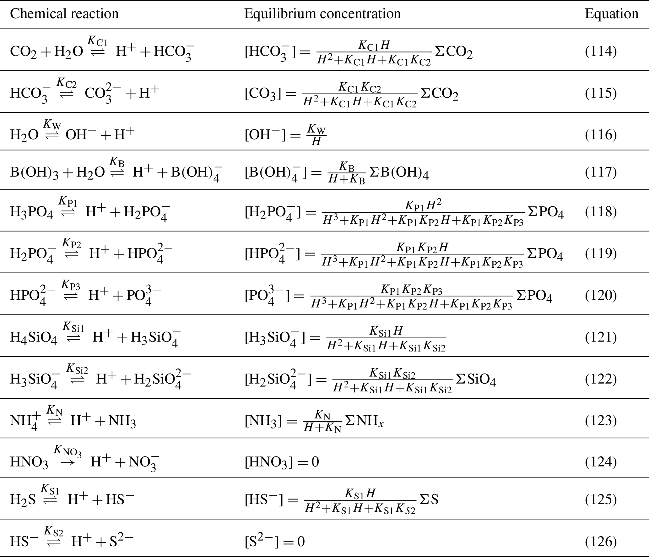
Table 3 lists the acid–base reactions taken into account in BAMHBI. This list includes the dissociation and protonation of carbonates (Eqs. 114, 115), water (Eq. 116), borates (Eq. 117), phosphates (Eqs. 118, 119 and (20), silicates (Eqs. 121 and 122), ammonium (Eq. (123)) and sulfide (Eqs. 125 and 126). Nitrate is assumed to be fully dissociated (Eq. 124) and in BAMHBI, the dissociation of nitrite, sulfates and fluoride is neglected.

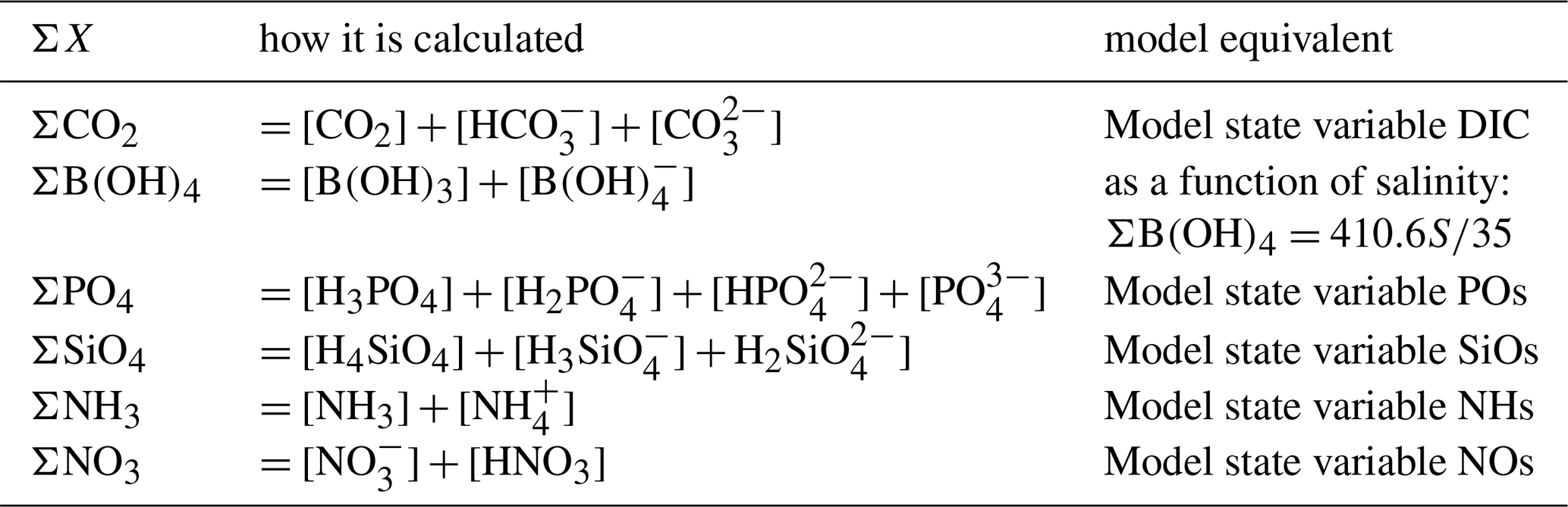
Chemical reactions presented in Table 3 generally occur at rates which, compared with the slow biogeochemical reactions that consume or produce protons, are fast enough to consider that they operate at equilibrium. In many of these reversible reactions the effective equilibrium is reached within seconds to minutes (Wolf-Gladrow and Riebesell, 1997, e.g.). The stoichiometric equilibrium speciation is expressed in terms of the total concentrations of species ($\sum X={\sum }_i\left[H_i{X}^{i-a}\right]$) (Table 4). These lump sums of concentrations (∑X) are (related to) model state variables. The equilibrium constants (K_*) are calculated as a function of temperature, salinity and pressure as given by Millero (1995) with typographical corrections according to Lewis and Wallace (1998); they are expressed on the total hydrogen ion pH scale. The borate concentrations are calculated as a function of salinity as described by Millero (1995).

Table 3 Main chemical reactions taken into account in the model that affect pH and the equilibrium concentrations (Soetaert et al., 2007). In the speciation relationships, H denotes [H⁺].

Table 4 Lump sums of concentrations.

Knowing the formulations for the equilibrium concentration of all the acid–base species, the dissociation constants and the lump sums of concentrations of species, the system of equations in Table 3 allows to solve the concentrations of all the ions and the proton concentration H⁺. As there are 16 unknowns, one more than the number of equations, an extra equation is required to find a unique solution. Usually, this additional equation is provided by TA:

$$\begin{array}{ll}{\displaystyle }\mathrm{TA}& {\displaystyle }=\left[{\mathrm{HCO}}_{\mathrm{3}}^{-}\right]+\mathrm{2}\left[{\mathrm{CO}}_{\mathrm{3}}^{\mathrm{2}-}\right]+\left[\mathrm{B}(\mathrm{OH}{)}_{\mathrm{4}}^{-}\right]+\left[{\mathrm{OH}}^{-}\right]\\ {\displaystyle }& {\displaystyle }+\left[{\mathrm{HPO}}_{\mathrm{4}}^{\mathrm{2}-}\right]+\mathrm{2}\left[{\mathrm{PO}}_{\mathrm{4}}^{\mathrm{3}-}\right]+\left[{\mathrm{H}}_{\mathrm{3}}{\mathrm{SiO}}_{\mathrm{4}}^{-}\right]\\ {\displaystyle }& {\displaystyle }+\mathrm{2}\left[{\mathrm{H}}_{\mathrm{2}}{\mathrm{SiO}}_{\mathrm{4}}^{\mathrm{2}-}\right]\\ {\displaystyle }& {\displaystyle }+\left[{\mathrm{NH}}_{\mathrm{3}}\right]+\left[{\mathrm{HS}}^{-}\right]+\mathrm{2}\left[{\mathrm{S}}^{\mathrm{2}-}\right]-\left[{\mathrm{H}}^{+}\right]-\left[{\mathrm{H}}_{\mathrm{3}}{\mathrm{PO}}_{\mathrm{4}}\right]\\ {\displaystyle }& {\displaystyle }-\left[{\mathrm{HSO}}_{\mathrm{4}}^{-}\right]-\left[\mathrm{HF}\right]-\left[{\mathrm{HNO}}_{\mathrm{3}}\right]-\left[{\mathrm{HNO}}_{\mathrm{2}}\right]\\ \text{(127)}& {\displaystyle }& {\displaystyle }-\mathrm{2}\left[{\mathrm{H}}_{\mathrm{2}}{\mathrm{SO}}_{\mathrm{4}}\right]\end{array}$$

In BAMHBI, the set of equations is completed by an additional equation for the “excess negative charge” (denoted Σ[−]) as described in Soetaert et al. (2007). This quantity expresses the excess of negative charge as the difference in concentrations of negative charges over positive charges (both multiplied by their charge) of the acid-base system given in Table 3:

$$\begin{array}{ll}{\displaystyle }\mathrm{\Sigma }[-]& {\displaystyle }=\left[{\mathrm{HCO}}_{\mathrm{3}}^{-}\right]+\mathrm{2}\left[{\mathrm{CO}}_{\mathrm{3}}^{\mathrm{2}-}\right]+\left[\mathrm{B}(\mathrm{OH}{)}_{\mathrm{4}}^{-}\right]+\left[{\mathrm{OH}}^{-}\right]\\ {\displaystyle }& {\displaystyle }+\left[{\mathrm{H}}_{\mathrm{2}}{\mathrm{PO}}_{\mathrm{4}}^{-}\right]+\mathrm{2}\left[{\mathrm{HPO}}_{\mathrm{4}}^{\mathrm{2}-}\right]+\mathrm{3}\left[{\mathrm{PO}}_{\mathrm{4}}^{\mathrm{3}-}\right]\\ {\displaystyle }& {\displaystyle }+\left[{\mathrm{H}}_{\mathrm{3}}{\mathrm{SiO}}_{\mathrm{4}}^{-}\right]+\mathrm{2}\left[{\mathrm{H}}_{\mathrm{2}}{\mathrm{SiO}}_{\mathrm{4}}^{\mathrm{2}-}\right]\\ {\displaystyle }& {\displaystyle }+\left[{\mathrm{NO}}_{\mathrm{3}}^{-}\right]+\left[{\mathrm{NO}}_{\mathrm{2}}^{-}\right]+\left[{\mathrm{F}}^{-}\right]+\left[{\mathrm{HS}}^{-}\right]+\mathrm{2}\left[{\mathrm{S}}^{\mathrm{2}-}\right]\\ \text{(128)}& {\displaystyle }& {\displaystyle }+\left[{\mathrm{HSO}}_{\mathrm{4}}^{-}\right]+\mathrm{2}\left[{\mathrm{SO}}_{\mathrm{4}}^{\mathrm{2}-}\right]-\left[{\mathrm{NH}}_{\mathrm{4}}^{+}\right]-\left[{\mathrm{H}}^{+}\right]\end{array}$$

If we assume that uptake of ions is compensated by uptake or release of protons (electroneutrality), Σ[−] is not impacted by changes in the concentrations of nitrate, nitrite, phosphate, ammonia/ammonium which is not the case of TA. It is straightforward to convert the Σ[−] to TA:

$$\begin{array}{ll}{\displaystyle }& {\displaystyle }\mathrm{TA}=\mathrm{\Sigma }[-]+\mathrm{\Sigma }{\mathrm{NH}}_{\mathrm{3}}-\mathrm{\Sigma }{\mathrm{NO}}_{\mathrm{3}}-\mathrm{\Sigma }{\mathrm{NO}}_{\mathrm{2}}\\ \text{(129)}& {\displaystyle }& {\displaystyle }-\mathrm{\Sigma }{\mathrm{PO}}_{\mathrm{4}}-\mathrm{2}\mathrm{\Sigma }{\mathrm{SO}}_{\mathrm{4}}-\mathrm{\Sigma }\mathrm{F}\end{array}$$

This equation needs to be adapted according to the protocol used to measure TA. BAMHBI does not solve for ΣSO₄, ΣF and ΣNO₂. Σ[−] is initialized with TA data using the conversion Eq. (129). Similarly, BAMHBI outputs TA as an ordinary variable that can be compared with observation.

The complete system of equations can be solved using a non-linear root–finding procedure, such as the Newton–Raphson technique for the H⁺ concentration and pH. Once pH is known, the equilibrium proportions between the different acids and bases can be calculated. For additional details, an extensive description of the carbonate model is provided by Soetaert et al. (2007) and Hofmann et al. (2008).

2.2.6 The Benthic module

If the Benthic module is included, BAMHBI solves the benthic compartment dynamics. Otherwise, the benthic compartment is considered as impermeable (i.e. when it reaches the bottom, the sinking material accumulates and is progressively degraded as in the water column). The benthic compartment is not vertically resolved but is described by a vertically integrated dynamic sediment model using the Level-3 approach proposed by Soetaert et al. (2001). Only the solid part is explicitly simulated by 5 state variables that include the vertically integrated content of a fast and slow reacting pools of organic C (resp. $S_{\mathrm{C}}^{\mathrm{f}}$ and $S_{\mathrm{C}}^{\mathrm{s}}$) and biogenic silica (resp. $S_{\mathrm{S}}^{\mathrm{f}}$ and $S_{\mathrm{S}}^{\mathrm{s}}$). The fifth state variable is the N:C ratio of the sedimentary organic matter (S_N:C) that is used to compute the sedimentary organic nitrogen (Table 1). The labile and refractory parts have the same stoichiometry. The sedimentary content of organic phosphorus is derived from the nitrogen content using the same N:P ratio as for the pelagic part.

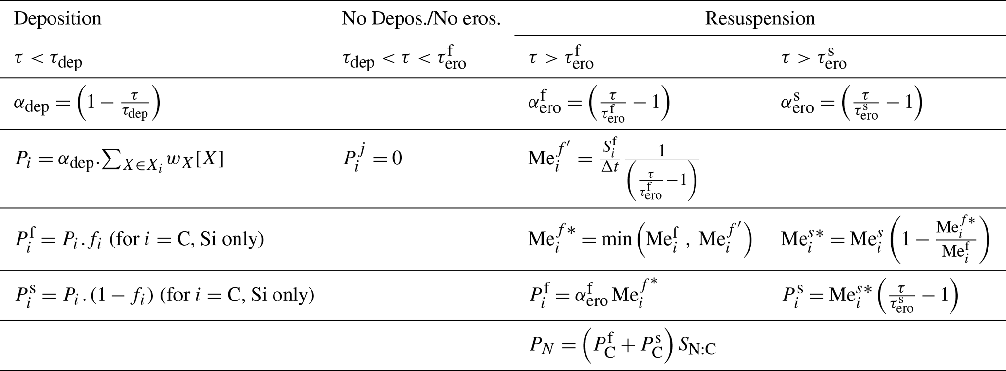
The sedimentary content of particulate organic carbon and biogenic silica (i.e., $S_{\mathrm{C}}^{\mathrm{f}}$, $S_{\mathrm{C}}^{\mathrm{s}}$, $S_{\mathrm{S}}^{\mathrm{f}}$ and $S_{\mathrm{S}}^{\mathrm{s}}$) increases due to sinking and deposition and decreases due to degradation, erosion/resuspension and burial (Eq. 24). $P_i^j$ denotes the net exchange between the sediment and the overlying water column of the degradable fraction j ($j=f,s$) of the particulate materials i ($i=\mathrm{C},\mathrm{Si}$). $P_i^j$ is the difference between the potential deposition and erosion rates and is computed according to the equations presented in Table 5. Based on the value of the bottom shear stress (i.e. τ) compared to thresholds values for deposition (i.e. τ_dep) and erosion (i.e. τ_ero), three situations are possible. For bottom shear stress below the threshold for deposition (i.e. τ_dep) only deposition occurs. The deposited materials is partitioned into the fast and slow degrading stock. For bottom shear stress in between the deposition and erosion threshold, there is neither deposition nor erosion. At high shear stress, larger than the erosion threshold, there is erosion of the stock. Because the slowly decaying stock is located deeper in the sediment and is more aggregated (Middelburg and Meysman, 2007), it is less easily resuspended than the fast degrading stock. Hence the slow decaying stock is resuspended when all the fast decaying stock is resuspended and the erosion threshold of the fast decaying stock (i.e. ${\mathit{\tau }}_{\mathrm{ero}}^{\mathrm{f}}$) is smaller than that of the slowly decaying fraction (i.e.  ${\mathit{\tau }}_{\mathrm{ero}}^{\mathrm{s}}$) (Table 5).

The bottom shear stress combines the stress due to the current and waves (Soulsby, 1997) and is computed at each time step according to Eqs. (136) to (141). The remineralization and dissolution rates are first order of the stock (Eqs. 130–131) and a part of the slowly decaying stock is buried (Eq. 132). The benthic carbon mineralization rate (D_C; Eq. 130) is derived from the sum of the degradation of the two biodegradable carbon fractions. The model estimated N:C ratio is used to derive the benthic nitrogen mineralization (D_N; Eq. 131).

Table 5 Computation of the net flux $P_i^j$ of particulate materials i (i= C, Si) of degradable fraction j ($j=f,s$) with [X]_i = [POC], [CDI], [PON, NDI], [SID], [SDI] for respectively i= C, N, Si.

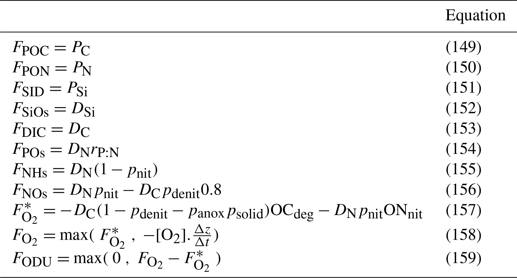
Porewater solutes are not explicitly simulated. The effect of benthic processes on pelagic dissolved inorganic constituents (i.e., NOs, NHs, O₂, POs, SiOs, DIC) is parameterized based on mass budget considerations and assuming that there is no storage in the sediment. The main reactions that affect the O₂ cycle in the sediment are (1) oxic mineralization (Eq. A1), (2) nitrification (Eq. A2) and (3) possible reoxydation of reduced substances produced during anoxic mineralization (Eq. A10). The main reactions affecting the sedimentary nitrogen cycle are (1) production of NHs in the degradation process and possible re-oxidation into NOs, (2) consumption of NOs during the denitrification and production of N₂.

The exchanges of solutes at the sediment-water interface are formulated as a function of variables p_Nit, p_Denit, p_Anox and p_SolidDepo defined in Table 2. The efflux of NHs equals the total organic nitrogen mineralisation (D_N) minus the amount of NHs oxidised by nitrification (i.e., p_Nit D_N; Eq. 155 in Table 7). The NOs efflux equals the production of NOs by nitrification minus its consumption by denitrification (i.e., 0.8 D_C p_Denit assuming a consumption of 0.8 mol of NOs per mole of organic carbon remineralized; see Eq. (156). The NOs efflux can be negative (i.e., NOs is consumed by the sediment) when the amount of NOs consumed by denitrifcation exceeds that produced by nitrification. The NHs efflux can also be negative when p_Nit>1 which occurs when the sediment mineralization is low and the NHs concentrations are high (Eq. 155). The O₂ flux to the sediment results from its consumption for the remineralisation and nitrification (respectively the first and second terms of Eq. 157 in Table 7). The consumed O₂ can be estimated from the amount of remineralized carbon (i.e., D_C) reduced by the amount of carbon degraded via denitrification and anoxic processes. O₂ is also consumed for the re-oxidation of the reduced substances that are produced by anoxic processes and are not deposited (i.e., p_Anox (1−pSolidDepo)). We assume that the efflux of SiOs equals the dissolution rate of particulate silicate, that of DIC is the carbon mineralization (D_C) and that of POs is computed from the nitrogen mineralization rate (D_N) assuming a constant Redfield P:N ratio (Eqs. 152, 153 and 154, resp.). The adsorption of NHs and POs is neglected.

The parameters p_Nit, p_Oxic and p_Anox are expressed as a function of the environmental conditions predicted by BAMHBI using meta-modelling. With that aim, Monte Carlo simulations (∼1000 runs) are performed with a one-dimensional vertically-resolved diagenetic model, OMEXDIA, implemented in the Black Sea by Wijsman et al. (2002). These Monte Carlo simulations are run over a range of environmental conditions (e.g. bottom water inorganic nutrient concentrations, mineralization rate, carbon flux to the bottom, organic matter reactivity, bioturbation and bio-irrigation rates, water depth) that are selected to cover the variability of the system. The vertically-resolved model-estimated nitrification and denitrification rates (resp. p_Nit D_N and p_Denit D_N) and p_Anox are regressed as a function of environmental variables (Eqs. 142–144) so that the vertically integrated model, used afterwards in BAMHBI, reproduces the results of the vertically resolved diagenetic model. The formulation of p_Nit, p_Oxic and p_Anox is derived before starting the three-dimensional simulations. The range of environmental conditions investigated to derive these formulations is quite large and the obtained formulations are very typical. The values of the p_Denit presents a peak at intermediate mineralization rate while p_Anox increases with the mineralization rate.p_SolidDepo is assumed to be constant (Table 6). The benthic model and its validation are described in details in Capet et al. (2016).

Remineralization-Dissolution

$$\begin{array}{ll}{\displaystyle }& {\displaystyle }{D}_i=\sum _{j=f,s}{k}_j{f}_i^j\left(T\right)S_i^j\text{with}{f}_i^j\left(T\right)=Q^{\frac{T-\mathrm{20}}{\mathrm{10}}}\\ \text{(130)}& {\displaystyle }& {\displaystyle }\text{with}i=\mathrm{C},\mathrm{Si}\text{and}j=f,s\text{(131)}& {\displaystyle }& {\displaystyle }{D}_{\mathrm{N}}=D_{\mathrm{C}}.S_{\mathrm{N}:\mathrm{C}}\end{array}$$

Burial

$$\begin{array}{}\text{(132)}& {\displaystyle }& {\displaystyle }{B}_i^{\mathrm{s}}=b_i.S_i^{\mathrm{s}}\text{with}i=\mathrm{C},\mathrm{Si}\text{(133)}& {\displaystyle }& {\displaystyle }{B}_i^{\mathrm{f}}=\mathrm{0}\end{array}$$

The mean first-order degradation rate

$$\begin{array}{}\text{(134)}& {\displaystyle }{\displaystyle }k={\displaystyle \frac{{\sum }_{j=f,s}{k}_j{f}_i^j\left(T\right)S_i^j}{{\sum }_{j=f,s}{S}_i^j}}\text{with}i=\mathrm{C},\mathrm{Si}\text{ and }j=f,s\end{array}$$

Shear stress due to currents and waves

$$\begin{array}{ll}\text{(135)}& {\displaystyle }& {\displaystyle }{\mathit{\tau }}_{\text{mean}}={\mathit{\tau }}_{\text{cur}}[\mathrm{1}+\mathrm{1.2}{\left({\displaystyle \frac{{\mathit{\tau }}_{\text{wave}}}{{\mathit{\tau }}_{\text{wave}}+{\mathit{\tau }}_{\text{cur}}}}\right)}^{\mathrm{3.2}}]\text{(136)}& {\displaystyle }& {\displaystyle }\mathit{\tau }=\sqrt{({\mathit{\tau }}_{\text{mean}}+{\mathit{\tau }}_{\text{wave}}\cos (\mathrm{\Phi }){)}^{\mathrm{2}}+({\mathit{\tau }}_{\text{wave}}\sin \left(\mathrm{\Phi }\right){)}^{\mathrm{2}}}{\displaystyle }& {\displaystyle }\text{where }\mathrm{\Phi }\text{ is the angle between waves and currents}\\ {\displaystyle }& {\displaystyle }{\mathit{\tau }}_{\mathrm{currents}}=\mathit{\rho }{c}_{\mathrm{db}}{U}^{\mathrm{2}}\\ \text{(137)}& {\displaystyle }& {\displaystyle }\text{with}{c}_{\mathrm{db}}=\left[{\displaystyle \frac{\mathrm{1}}{\mathit{\kappa }}}\right(\mathrm{1}+\log {\displaystyle \frac{z_{\mathrm{0}}}{\mathrm{\Delta }{z}_{\mathrm{bottom}}}}){]}^{-\mathrm{2}}{\displaystyle }& {\displaystyle }\text{or set to constant value as in NEMO}\\ {\displaystyle }& {\displaystyle }\left(\mathtt{\text{ln\_non\_lin}}\text{ namelist option}\right)\\ \text{(138)}& {\displaystyle }& {\displaystyle }{\mathit{\tau }}_{\mathrm{waves}}=\mathrm{0.5}\mathit{\rho }{f}_{\mathrm{w}}{U}_{\mathrm{w}}^{\mathrm{2}}{\displaystyle }& {\displaystyle }\text{with}{U}_{\mathrm{w}}\text{is the maximum horizontal orbital wave velocity}\\ \text{(139)}& {\displaystyle }& {\displaystyle }{f}_{\mathrm{w}}=max(f_{\mathrm{wr}},f_{\mathrm{ws}}){\displaystyle }& {\displaystyle }\text{The bottom friction is the maximum of rough}\\ {\displaystyle }& {\displaystyle }\text{and smooth bed friction}\\ {\displaystyle }& {\displaystyle }{f}_{\mathrm{wr}}=\mathrm{0.237}{\left({\displaystyle \frac{A}{k_s}}\right)}^{-\mathrm{0.52}}\text{with}A={\displaystyle \frac{U_{w}T}{\mathrm{2}\mathit{\pi }}}\\ \text{(140)}& {\displaystyle }& {\displaystyle }\text{and}{k}_s=\mathrm{2.5}{d}_{\mathrm{50}}{\displaystyle }& {\displaystyle }{f}_{\mathrm{ws}}=B{R}_{\mathrm{w}}^{-N}\text{where}{R}_{\mathrm{w}}\text{ is the Reynolds number}\\ {\displaystyle }& {\displaystyle }\text{if}{R}_{\mathrm{w}}<\mathrm{5}{\mathrm{10}}^{-\mathrm{5}}\text{the flow is laminar and}B=\mathrm{2},N=\mathrm{0.5}\\ {\displaystyle }& {\displaystyle }\text{if}{R}_{\mathrm{w}}>\mathrm{5}{\mathrm{10}}^{-\mathrm{5}}\text{the flow is turbulent and}B=\mathrm{0.0521},\\ \text{(141)}& {\displaystyle }& {\displaystyle }N=\mathrm{0.187}\end{array}$$

Bulk Parameterization

$$\begin{array}{ll}{\displaystyle }& {\displaystyle }\ln (p_{\mathrm{Nit}}.D_{\mathrm{N}})=-\mathrm{6.280}-\mathrm{0.286}(\ln D_{\mathrm{C}}{)}^{\mathrm{2}}\\ {\displaystyle }& {\displaystyle }+\mathrm{0.127}(\ln D_{\mathrm{C}}{)}^{\mathrm{3}}+\mathrm{0.006}(\ln D_{\mathrm{C}}{)}^{\mathrm{4}}\\ {\displaystyle }& {\displaystyle }+\mathrm{0.098}\left(\ln D_{\mathrm{C}}\right).\ln \left(\right[{\mathrm{O}}_{\mathrm{2}}\left]\right)+\mathrm{0.202}(\ln D_{\mathrm{C}}{)}^{\mathrm{2}}.\ln (\left[{\mathrm{O}}_{\mathrm{2}}\right])\\ {\displaystyle }& {\displaystyle }-\mathrm{0.021}(\ln D_{\mathrm{C}}{)}^{\mathrm{3}}.\ln (\left[{\mathrm{O}}_{\mathrm{2}}\right])-\mathrm{0.031}(\ln D_{\mathrm{C}}{)}^{\mathrm{2}}.\left(\ln \right(\left[{\mathrm{O}}_{\mathrm{2}}\right]){)}^{\mathrm{2}}\\ {\displaystyle }& {\displaystyle }-\mathrm{0.066}\ln \left(D_{\mathrm{C}}\right).\ln \left([\mathrm{NHs}\right])+\mathrm{0.009}(\ln D_{\mathrm{C}}{)}^{\mathrm{2}}.\ln \left(\right[\mathrm{NOs}\left]\right)\\ {\displaystyle }& {\displaystyle }+\mathrm{0.823}\ln \left(\right[{\mathrm{O}}_{\mathrm{2}}\left]\right)-\mathrm{0.028}\left(\ln \right(\left[{\mathrm{O}}_{\mathrm{2}}\right]){)}^{\mathrm{2}}\\ {\displaystyle }& {\displaystyle }-\mathrm{0.012}\ln \left(\right[{\mathrm{O}}_{\mathrm{2}}\left]\right).\ln \left(\right[\mathrm{NHs}\left]\right)\\ \text{(142)}& {\displaystyle }& {\displaystyle }+\mathrm{0.119}\ln \left(\right[\mathrm{NHs}\left]\right)+\mathrm{0.015}\left(\ln \right(\left[\mathrm{NHs}\right]){)}^{\mathrm{2}}{\displaystyle }& {\displaystyle }\ln (p_{\mathrm{Denit}}.D_{\mathrm{C}})=-\mathrm{5.475}-\mathrm{0.786}(\ln D_{\mathrm{C}}{)}^{\mathrm{2}}\\ {\displaystyle }& {\displaystyle }+\mathrm{0.662}(\ln D_{\mathrm{C}}{)}^{\mathrm{3}}+\mathrm{0.042}(\ln D_{\mathrm{C}}{)}^{\mathrm{4}}\\ {\displaystyle }& {\displaystyle }+\mathrm{0.064}\left(\ln D_{\mathrm{C}}\right).\left(\ln \right(\left[{\mathrm{O}}_{\mathrm{2}}\right]\left)\right)+\mathrm{0.794}(\ln D_{\mathrm{C}}{)}^{\mathrm{2}}.(\ln \left(\right[{\mathrm{O}}_{\mathrm{2}}\left]\right))\\ {\displaystyle }& {\displaystyle }-\mathrm{0.082}(\ln D_{\mathrm{C}}{)}^{\mathrm{3}}.(\ln \left(\right[{\mathrm{O}}_{\mathrm{2}}\left]\right))-\mathrm{0.122}(\ln D_{\mathrm{C}}{)}^{\mathrm{2}}.\left(\ln \right(\left[{\mathrm{O}}_{\mathrm{2}}\right]){)}^{\mathrm{2}}\\ {\displaystyle }& {\displaystyle }+\mathrm{0.077}\left(\ln \right(\left[{\mathrm{O}}_{\mathrm{2}}\right]){)}^{\mathrm{2}}-\mathrm{0.155}(\ln \left(\right[{\mathrm{O}}_{\mathrm{2}}\left]\right)).(\ln \left(\right[[\mathrm{NOs}\left]\right))\\ \text{(143)}& {\displaystyle }& {\displaystyle }+\mathrm{0.875}\ln \left(\right[[\mathrm{NOs}\left]\right)+\mathrm{0.046}\left(\ln \right(\left[\right[\mathrm{NOs}\left]\right){)}^{\mathrm{2}}{\displaystyle }& {\displaystyle }{p}_{\mathrm{anox}}=\mathrm{1.056}-\mathrm{0.132}\left(\ln D_{\mathrm{C}}\right)+\mathrm{0.005}(\ln D_{\mathrm{C}}{)}^{\mathrm{4}}\\ {\displaystyle }& {\displaystyle }+\mathrm{0.057}\left(\ln D_{\mathrm{C}}\right).\left(\ln \right(\left[{\mathrm{O}}_{\mathrm{2}}\right]\left)\right)-\mathrm{0.017}(\ln D_{\mathrm{C}}{)}^{\mathrm{2}}.(\ln \left(\right[{\mathrm{O}}_{\mathrm{2}}\left]\right))\\ \text{(144)}& {\displaystyle }& {\displaystyle }-\mathrm{0.008}\left(\ln \right(\left[{\mathrm{O}}_{\mathrm{2}}\right]){)}^{\mathrm{2}}\end{array}$$

Table 6 Parameters values for biological processes.

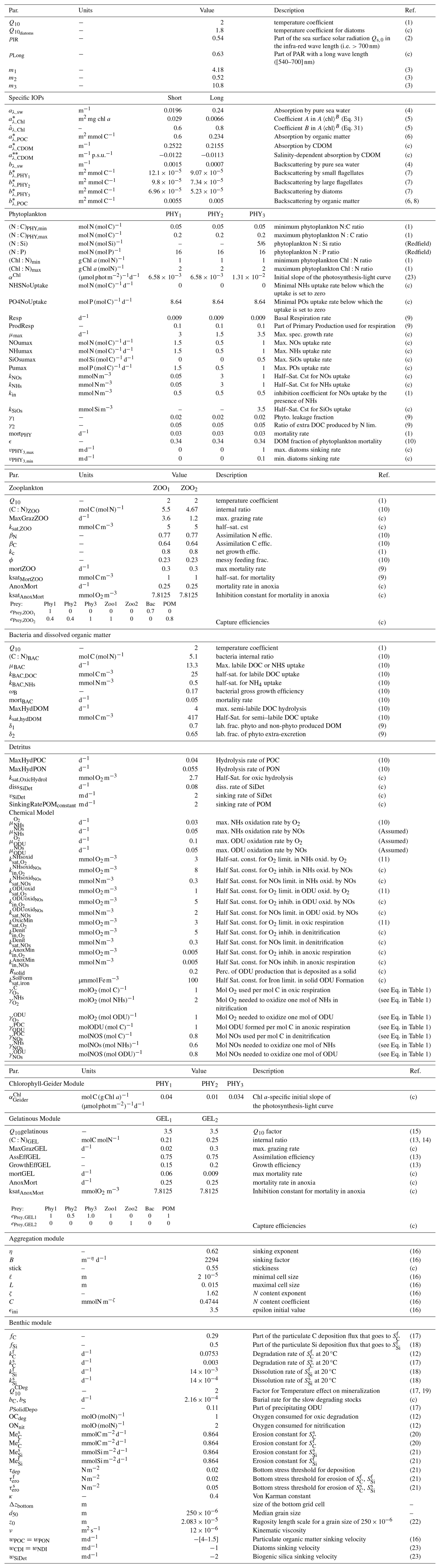
(c) after calibration. References: (1) Soetaert et al. (2001), (2) Mobley et al. (2004), (3) Lee et al. (2005), (4) Smith and Baker (1981), (5) Bricaud et al. (1995), (6) Neukermans et al. (2012), (7) Vaillancourt et al. (2004), (8) Doerffer and Schiller (2007), (9) Van den Meersche et al. (2004), (10) Anderson and Pondaven (2003), (11) Soetaert et al. (1996), (12) Muramoto et al. (1991), (13) Lancelot et al. (2002), (14) Nakamura (1998), (15) Kremer (1977), (16) Kriest (2002), (17) Wijsman et al. (2002), (18) calibrated values based on Khalil et al. (2007), (19) Van Cappellen et al. (2002), (20) Stanev and Kandilarov (2012), (21) Capet et al. (2016), (22) Gayer et al. (2006), (23) Grégoire et al. (2008).

Table 7 Benthic-pelagic boundary conditions.

3 Horizontal interfaces

3.1 Air-sea interface

Gases, CO₂ and O₂, are exchanged at the air-sea interface. Net CO₂ flux at the air-sea interface (AirSeaCO₂Flux) depends on the difference in partial pressure of CO₂ (pCO₂) between air (pCO_2,air) and the surface water (pCO_2,water), the solubility coefficient K₀(S,T) and the gas transfer velocity k(wind). k(wind) is parameterized as a function of the wind speed with the formulation of Wanninkhof (1992):

$$\begin{array}{ll}{\displaystyle }& {\displaystyle }{\text{AirSeaCO}}_{\mathrm{2}}\text{Flux}=K_{\mathrm{0}}(S,T)k\left(\mathrm{wind}\right)\\ \text{(145)}& {\displaystyle }& {\displaystyle }({\mathrm{pCO}}_{\mathrm{2},\mathrm{air}}-{\mathrm{pCO}}_{\mathrm{2},\mathrm{water}}){\displaystyle }& {\displaystyle }k\left(\mathrm{wind}\right)=\mathrm{0.31}{\mathrm{wind}}^{\mathrm{2}}{\displaystyle \frac{\mathrm{1}}{\sqrt{S_c/\mathrm{660}}}}\\ {\displaystyle }& {\displaystyle }\text{with}{S}_c=\mathrm{2073.1}-\mathrm{125.62}T+\mathrm{3.6276}{T}^{\mathrm{2}}\\ \text{(146)}& {\displaystyle }& {\displaystyle }-\mathrm{0.043219}{T}^{\mathrm{3}}\end{array}$$

where S_c is the Schmidt number.

The net O₂ flux at the air-sea interface (AirSeaO₂Flux) depends on the difference in the O₂ saturation concentration (O_2,sat) and the surface water O₂ concentration (O_2,water), the solubility coefficient K₀(S,T) and the gas transfer velocity k(wind) which is parameterized as a function of the wind speed with the formulation of Ho et al. (2006):

$$\begin{array}{ll}\text{(147)}& {\displaystyle }& {\displaystyle }{\mathrm{AirSeaO}}_{\mathrm{2}}\mathrm{Flux}=k\left(\mathrm{wind}\right)({\mathrm{O}}_{\mathrm{2},\mathrm{sat}}-{\mathrm{O}}_{\mathrm{2},\mathrm{water}}){\displaystyle }& {\displaystyle }k\left(\mathrm{wind}\right)=\mathrm{0.266}{\mathrm{wind}}^{\mathrm{2}}{\displaystyle \frac{\mathrm{1}}{\sqrt{S_c/\mathrm{660}}}}\\ {\displaystyle }& {\displaystyle }\text{with}{S}_c=\mathrm{1953.4}-\mathrm{128.00}T+\mathrm{3.9918}{T}^{\mathrm{2}}\\ \text{(148)}& {\displaystyle }& {\displaystyle }-\mathrm{0.050091}{T}^{\mathrm{3}}\end{array}$$

where S_c is the Schmidt number.

Additionally the model includes the possibility to consider the deposition of dissolved inorganic nitrogen and phosphorus. None of the other biogeochemical state variables is exchanged across the air-sea interface.

Table 8 List of available options: name and definition.

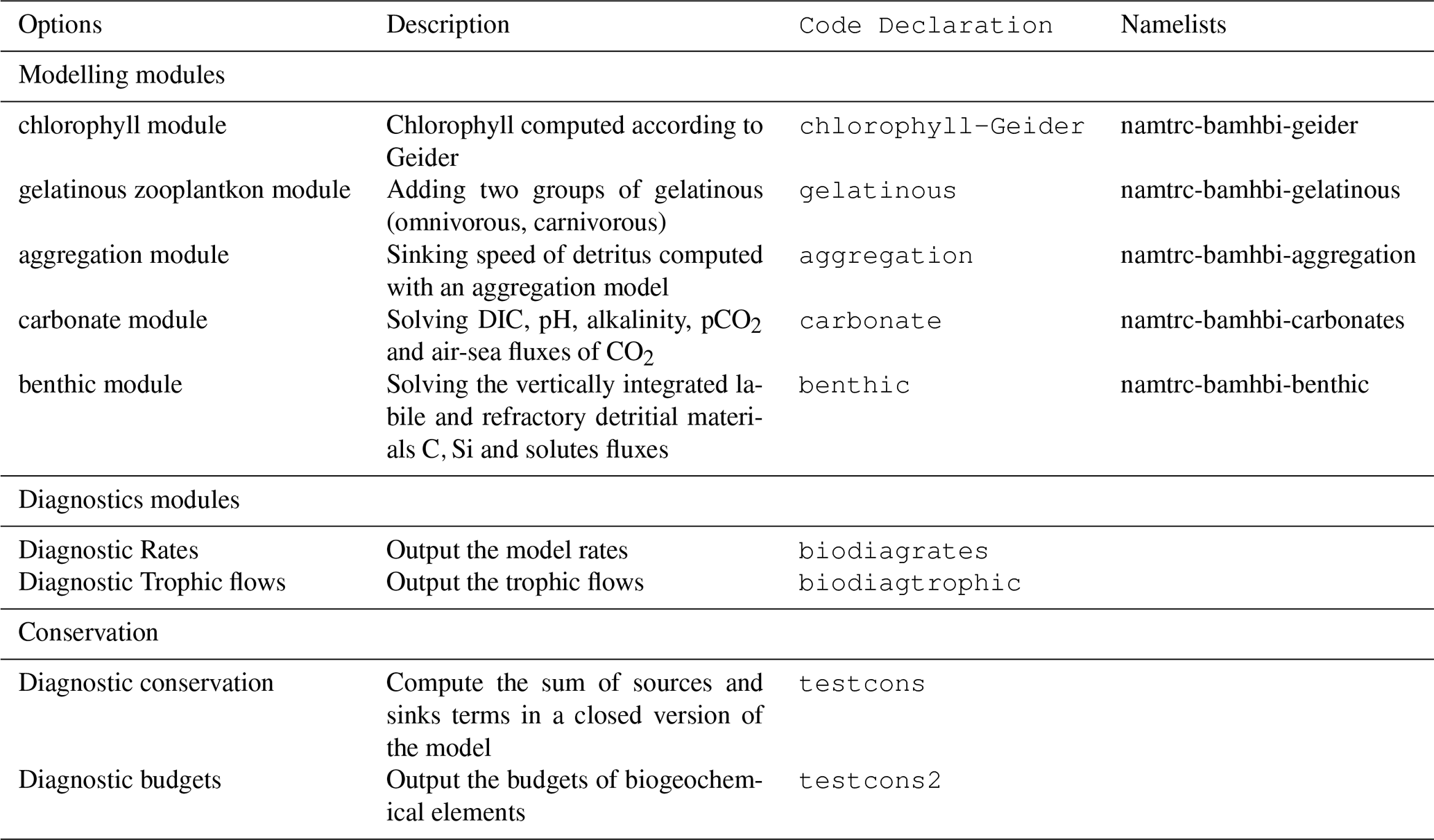
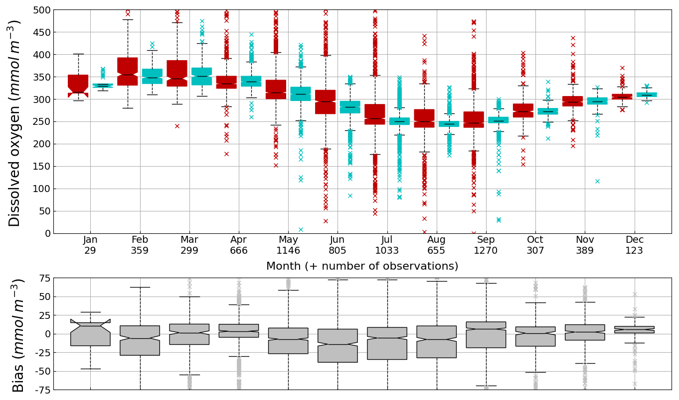
Figure 6 Seasonal cycle, average over 1980–2002, of surface (0–10 m) O₂ concentration (median, P₂₅ and P₇₅ values) over the Black Sea northwestern shelf simulated (cyan) and observed (red). Observations have been extracted from the World Ocean Database (Mishonov et al., 2024). Their number is indicated in the top figure. Model results are interpolated at the data points.

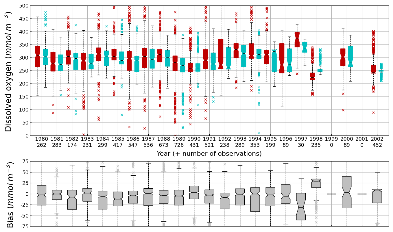
Figure 7 Interannual cycle of surface (0–10 m) O₂ concentration (median, P₂₅ and P₇₅ values) over the Black Sea northwestern shelf simulated (cyan) and observed (red) (top panel) and median of the bias between the model (cyan) and observations (red) estimates (bottom panel). Observations have been extracted from the World Ocean Database (Mishonov et al., 2024). Their number is indicated in the top figure. Model results are interpolated at the data points.

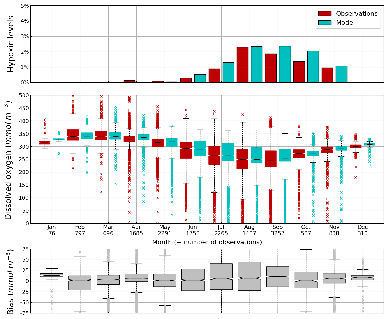
Figure 8 Seasonal cycle, average over 1980–2002, of the percentage of shelf area affected by bottom hypoxia (i.e. O₂< 63 µmol L⁻¹) (top panel), bottom (10–45 m) O₂ concentration (median, P₂₅ and P₇₅ values) (middle panel) and median of the bias between the model (cyan) and observations (red) estimates. Observations have been extracted from the World Ocean Database (Mishonov et al., 2024). Their number is indicated in the middle figure. Model results are interpolated at the data points.

3.2 Water-sediment interface

By default, the bottom is considered as frozen. The sedimenting particles accumulate on the bottom and are degraded in the bottom layer of the pelagic model. When the benthic module is activated, a sedimentary box is considered as explained in Sect. 2.2.6. Table 7 lists the pelagic variables that have a non-zero flux imposed at the sediment-water interface. These variables are all the sedimenting and dissolved inorganic modelled components. When the flux of solutes can be directed towards the sediments (which is always the case for O₂ and may occur for NHs and NOs) it may happen that the computed influx exceeds the availability of solutes in the last box of the pelagic model. This is because the meta-modelling formulation does not directly depend on the availability of the solute in the last box of the pelagic model. In that case, the modelled influx is adjusted to consume the quantity of solute in the bottom box (i.e. $\left[\mathrm{Solute}\right]\frac{\mathrm{\Delta }z}{\mathrm{\Delta }t}$). Then, for O₂ the excess consumption is converted into a release of ODU (Eq. 158) while for NHs and NOs, the parameters (respectively p_Nit, p_Denit) are adjusted for not exceeding the available amount and all the fluxes are recomputed to preserve mass conservation. It should be noted that these adjustments are rare.

4 Implementation

The BAMHBI model comes as an independent library. The source and sink terms of the pelagic variables (and benthic variables if the benthic module is activated) are computed by BAMHBI in the bamhbi.F90 module written in Fortran 90. BAMHBI parameters are declared in bamhbi_params.F90. Each optional module has its own namelist, variables declaration file (bamhbi_optionalmodule_vars.F90, e.g. bamhbi_alkalinity_vars.F90) and FORTRAN code (bamhbi_optionalmodule.F90, e.g. bamhbi_alkalinity.F90). All of these files include the BAMHBI.h90 header file containing pre-processor directives enabling or disabling specific parts of the code such as described in Sect. 4.2.

The time integration is done externally. BAMHBI needs to be forced by temperature, salinity, mixing coefficients and, in a three-dimensional setting, currents. Most of the time these forcings are provided by an ocean physical model. BAMHBI has already been coupled in 1D with GOTM (Grégoire et al., 2008), in 3D with the GHER model (Capet et al., 2013), and in 1D and 3D with the “Nucleus for European Modelling of the Ocean” (NEMO). As much as possible, BAMHBI is written to be easily coupled with hydrodynamical models without substantial adaptations. The notation (e.g. names of loop indices and physical variables) respects the NEMO conventions. For each physical model, an interface module has to “translate” the variable names between the respective physical model and BAMHBI. Here we describe the time integration of BAMHBI in NEMO.

4.1 Coupling with NEMO

The definition of the variables in the BAMHBI code follows the NEMO nomenclature (e.g. jpi for the dummy loop index in the longitudinal direction, e3t for the height of the grid cells, tr for the biogeochemical variables). The interface module between NEMO and BAMHBI, called bamhbi_driver_nemo.F90 is thus relatively short. The complete BAMHBI source code is stored in the NEMO MY_SRC sub-directory and through bamhbi_driver_nemo.F90, it uses all the required variables (e.g. grids, masks, physical variables (active tracers), biogeochemical pelagic and benthic variables (passive tracers), surface wind stress, surface radiation, bottom wave stress).

The calls to the BAMHBI subroutines are done in the NEMO trc_sms_my_trc subroutine. At each time step, some preliminary operations are done (such as resetting all source and sinks to zero), then for each biogeochemical variable the sources and sinks are computed, and from that the source minus sinks term (i.e. trends in NEMO's terminology).

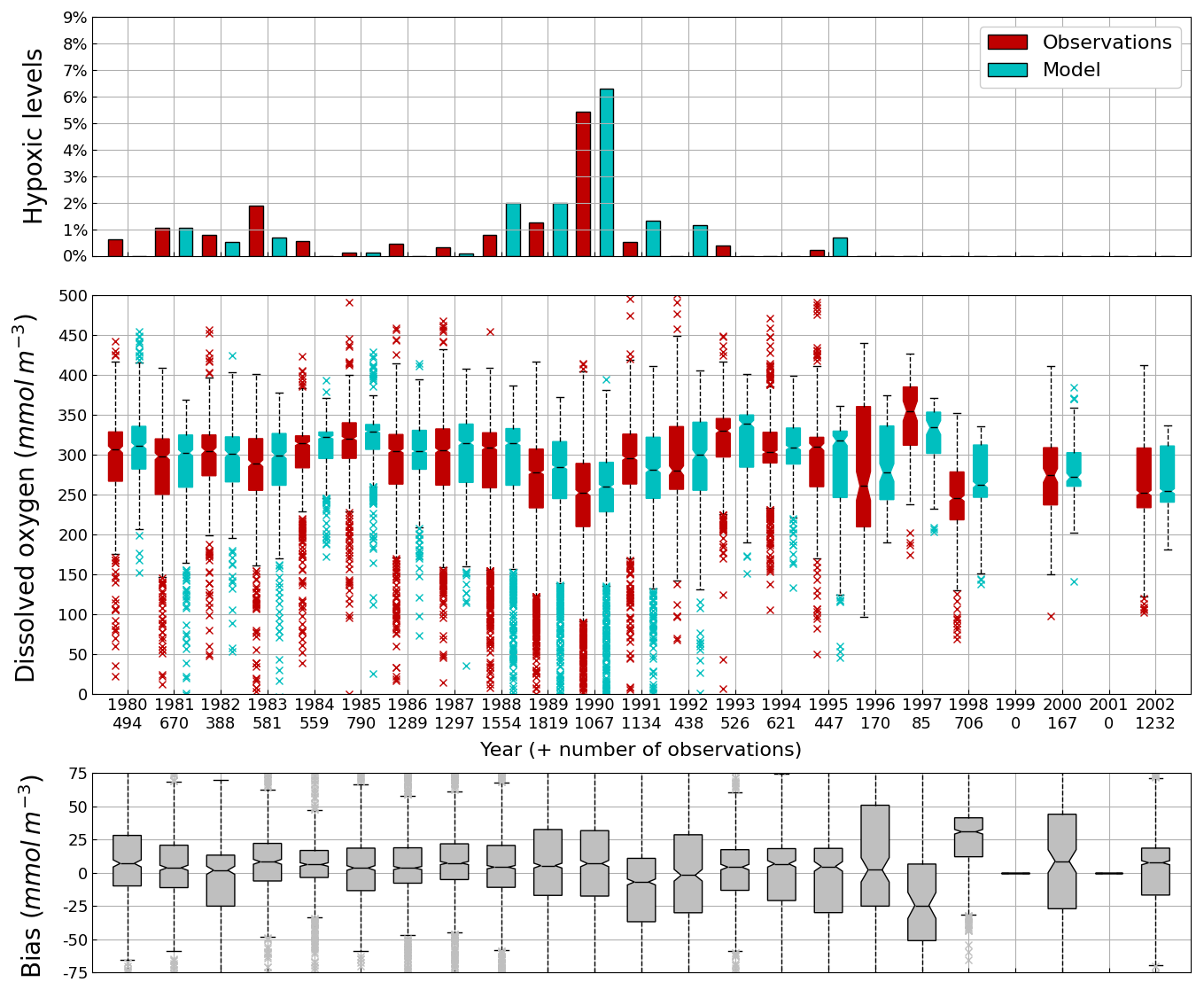
Figure 9 Interannual cycle of the percentage of shelf area affected by bottom hypoxia (i.e. O₂< 63 µmol L⁻¹) (top panel), bottom (10–45 m) O₂ concentration (median, P₂₅ and P₇₅ values) (middle panel) and median of the bias between the model (cyan) and observations (red) estimates. Observations have been extracted from the World Ocean Database (Mishonov et al., 2024). Their number is indicated in the middle figure. Model results are interpolated at the data points.

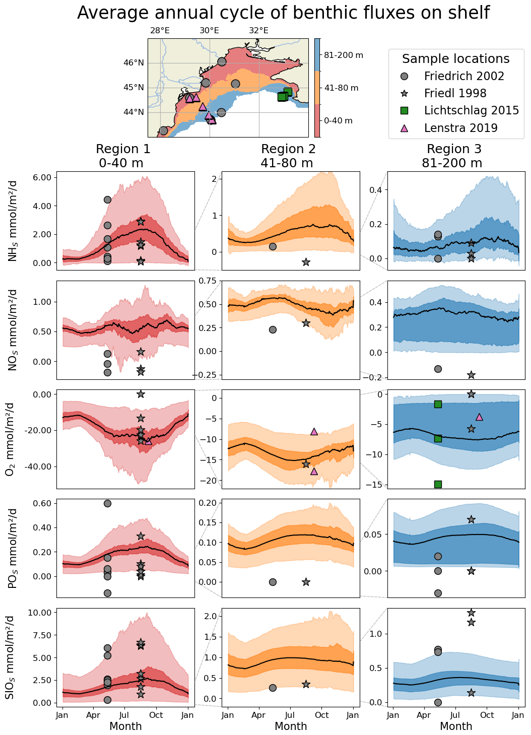
Figure 10 Average (1990–1999) seasonal cycle of the benthic fluxes of (from the first to the last row) NHs, NOs, O₂, POs, SiOs observed (symbols) for regions of different bathymetry ranges and simulated by BAMHBI (continuous lines with the 25th and 75th (resp. 2.5th and 97.5th) percentiles superimposed in dark (resp. light) color). The distribution of the different regions as well as the data collection sites are shown in the top of the figure (first row). The sampling sites of Friedl et al. (1998) and Friedrich et al. (2002) are similar but are collected respectively in August 1995 (stars) and May 1997 (circles). In addition, data published by Lichtschlag et al. (2015) and Lenstra et al. (2019) were used.

4.2 Compilation Options

The BAMHBI.h90 header file contains pre-processor directives enabling or disabling specific parts of the code. Available options include the modelling modules described in details in Sect. 2.2 and the estimation of model diagnostics described here below. All the compiling options are listed in Table 8.

4.2.1 Mass conservation

Compiling BAMHBI with option “testcons” allows to check that the model is conservative in terms of C, N, Si, P and O₂. This option cancels the calls to routines that are the net sources and sinks for the model (i.e. denitrification, ANAMMOX, nitrate reduction by ODU are losses of nitrogen since N₂ is not explicitly modelled). It then checks that at each time step the sum of the biogeochemical sources and sinks (i.e. $\frac{\partial y}{\partial t}{|}_{\mathrm{Bio}}$) equals zero. With the option “testcons2” the inventory over the modelled domain of each chemical currency (i.e. C, N, Si, P and O₂) is computed closing the system (i.e. removing its interactions with the outside world). It remains the user responsibility to cancel fluxes at open boundaries, rivers, and atmosphere. For example, when BAMHBI is coupled with NEMO, these fluxes are specified in NEMO's namelist_top_cfg file respectively in the BDY, SBC and CBC parts.

4.2.2 Clipping

When integrating the biogeochemical variables, it may happen that negative concentrations are generated, when for instance, the sink term of a given biogeochemical variable exceeds its stock. These negative concentrations are not realistic and may create instabilities. Then, before computing the sources and sinks terms, negative state variables are set to a small value specified in the BAMHBI parameters (e.g. 10⁻¹²) and the added material is computed over the whole domain to check its order of magnitude compared to the total mass. When BAMHBI is coupled to NEMO, the BAMHBI clipping procedure can be replaced with NEMO's trc_rad routine. This clips the biogeochemical variables after integration of the total trend, obtained as the sum of the source and sinks (computed by BAMHBI) and the transport (advection and diffusion, computed by BAMHBI).

4.2.3 Diagnostics

A list of diagnostics are proposed to estimate model rates and trophic interactions. These sets of diagnostics can be computed by activating respectively the options “biodiagrates” and “biodiagtrophic”.

5 BAMHBI Applications

This section describes two applications of BAMHBI to simulate the Black Sea biogeochemistry. One of them describes the use of the model to estimate benthic-pelagic fluxes and oxygen over the northwestern shelf. In the second application, the Chl a, oxygen and nitrate dynamics are simulated and compared with ARGO and ship data in the deep sea.

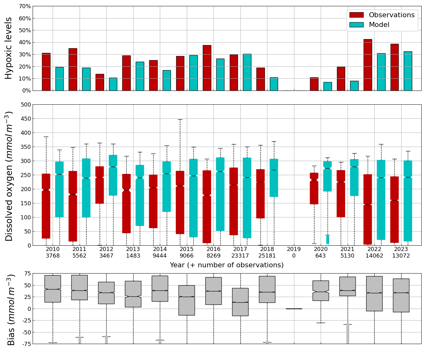
Figure 11 Average (2010–2023) monthly cycle of, the percentage of points with hypoxia (i.e. O₂< 63 µmol L⁻¹) (top panel), the concentration of O₂ (0–100 m) observed by Argos (red) and simulated by BAMHBI (cyan) median values with the 25th and 75th (resp. 2.5th and 97.5th) percentiles limiting the color bars (resp. dotted lines) and (bottom figure) the median value of the bias.

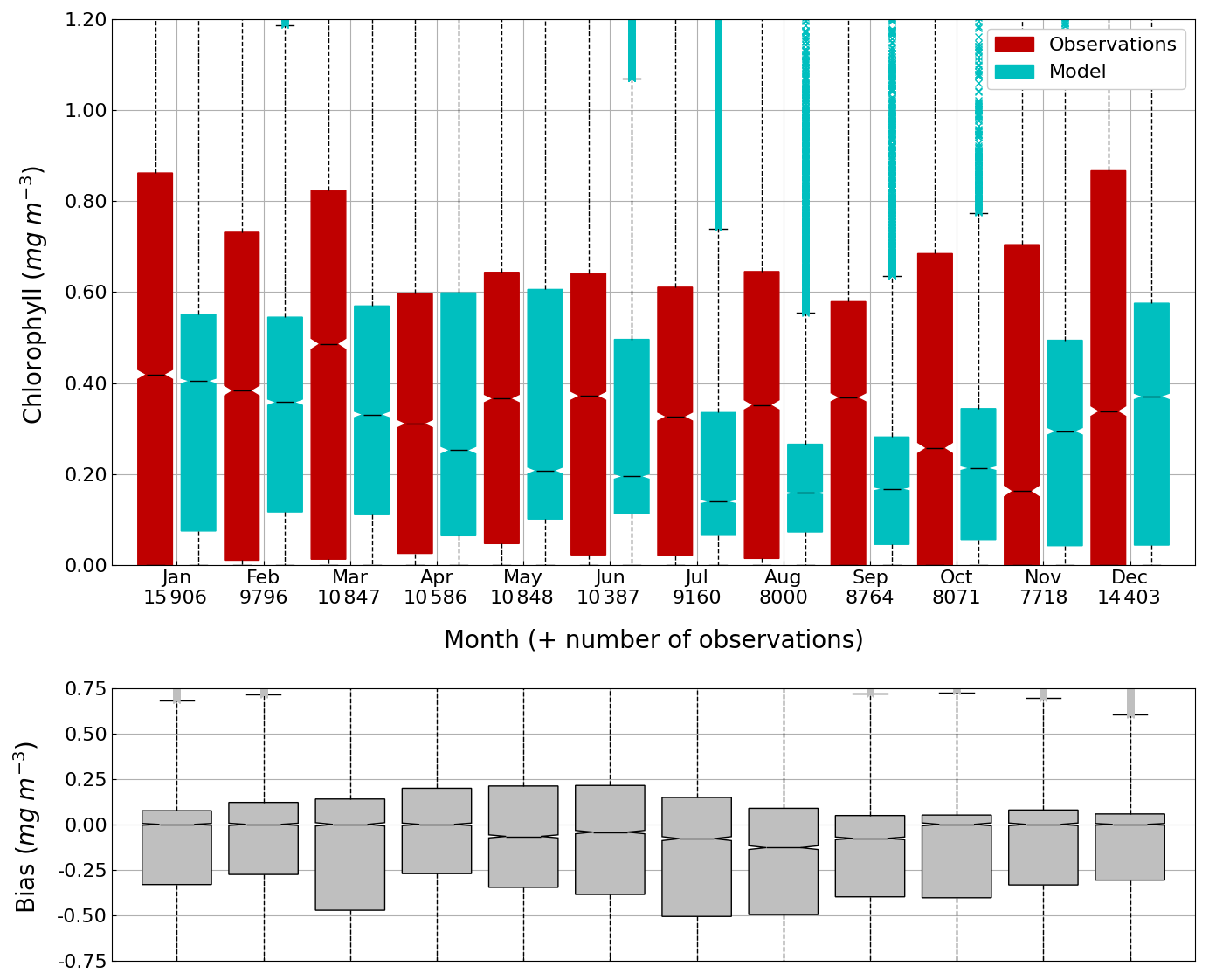
Figure 12 Average (2013–2023) seasonal cycle of (top figure) the concentration of Chl a (0–100 m) observed by Argos (red) and simulated by BAMHBI (cyan) median values with the 25th and 75th (resp. 2.5th and 97.5th) percentiles limiting the color bars (resp. dotted lines) and (bottom figure) the median value of the bias.

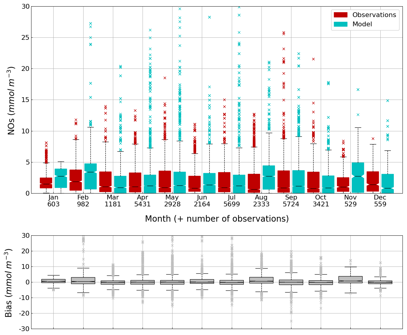
Figure 13 Seasonal cycle, average over 1980–2002, of the NOs concentration (median, P₂₅ and P₇₅ values) (top panel) and median of the bias between the model (cyan) and observations (red) estimates (bottom panel) over the deep basin. Observations come from both the World Ocean Database (Mishonov et al., 2024) and European Marine Observation and Data Network (EMODnet). Their number is indicated under the top figure. Model results are interpolated at the data points.

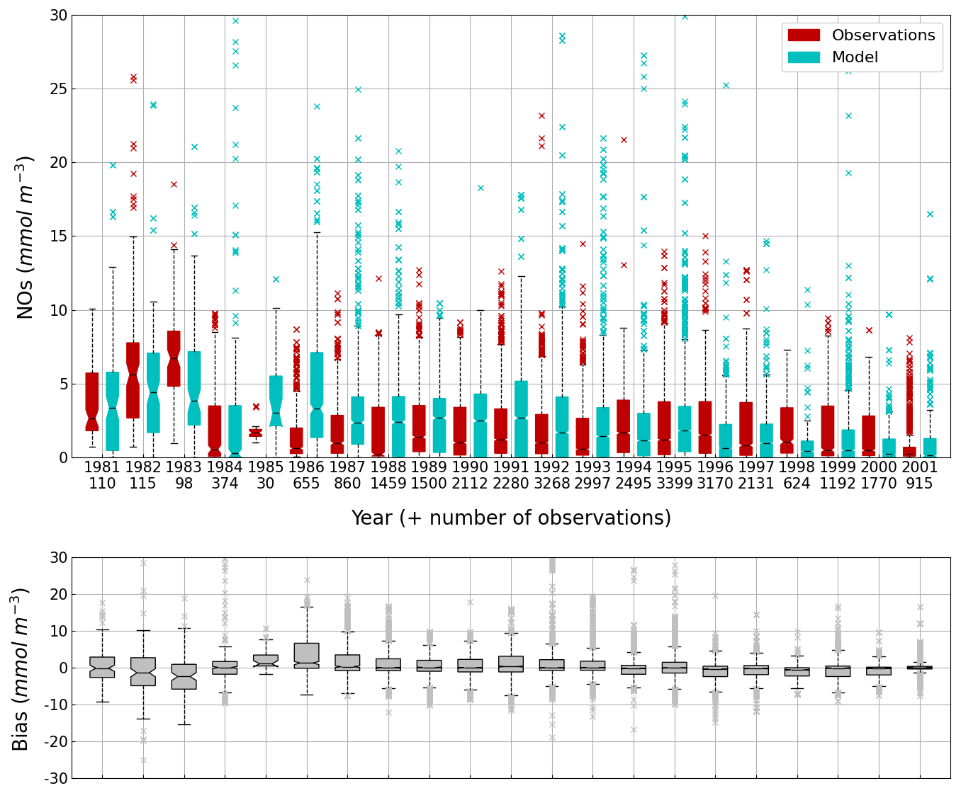
Figure 14 Interannual cycle of the NOs concentration (median, P₂₅ and P₇₅ values) (top panel) and median of the bias between the model (cyan) and observations (red) estimates (bottom panel) over the deep basin. Observations come from both the World Ocean Database (Mishonov et al., 2024) and European Marine Observation and Data Network (EMODnet). Their number is indicated under the top figure. Model results are interpolated at the data points.

In these two applications BAMHBI is online coupled with NEMO. At each NEMO 3D time step biogeochemical variables are integrated and transported (by advection and diffusion) in the NEMO framework. At the air-sea interface, the coupled model is forced by ERA-5 data (Hersbach et al., 2020) that are used to estimate the heat and energy exchanges using bulk formulations. Precipitation and nutrients fluxes (i.e. NOs, NHs, POs) are also imposed and the exchanges of O₂ and CO₂ are computed as described in Sect. 3. For the other biogeochemical variables, a zero flux condition is imposed. At the water-sediment interface, the shear stress due to current and waves is imposed. The waves are imposed as an external forcing from Stanev and Kandilarov (2012). For biogeochemical variables boundary conditions are described in Sect. 3. The physics is initialized from rest with typical vertical profiles of temperature and salinity. A spin-up of 15 years is performed forced by climatological atmospheric forcings. The initial conditions of inorganic components like NOs, NHs, POs, SiOs, O₂, ODU,DIC, TA, and pH are expressed on a density scale using typical profiles. For the other biogeochemical variables, homogeneous profiles with very low values are used. In the sediment, the slowly and fast reacting components are initialized with a 5-year averaged deposition rate divided by the first-order averaged decay rates. A new spin-up of 15 years is then performed with the coupled model to adjust the initial biogeochemical conditions to the dynamics. The model starts in 1950.

5.1 Case Study: shelf hypoxia and benthic–pelagic coupling

Oxygen is the modeled state variable for which there is the largest amount of observation. At the surface, the dynamics of oxygen is governed essentially by air-sea exchanges that tend to bring surface waters at equilibrium. In winter, the cooling of surface waters increases the saturation value. Waters are undersaturated and oxygen is transferred from the atmosphere to the sea. When waters progressively warm, the saturation concentration decreases and there is an outgassing of oxygen from the sea to the atmosphere. The seasonal cycle of surface oxygen over the Black Sea northwestern shelf is quite well represented as shown in Fig. 6 with a median bias lower than 15 µmol L⁻¹. The interannual cycle is also very well represented with a median bias close to zero except during 1997 and 1998 where it reaches ≃ 25 µmol L⁻¹ (Fig. 7). Since the early 80s, in response to eutrophication, the Black Sea northwestern shelf has been affected by bottom hypoxia (Zaitsev, 1993; Mee et al., 2005; Capet et al., 2013, e.g.,). Bottom hypoxia has affected benthic communities and the coupling of the benthic and pelagic compartments. In this case study, the capability of BAMHBI to generate bottom shelf hypoxia and benthic–pelagic fluxes is demonstrated. Figures 8 and 9 compare the simulated and observed bottom oxygen concentrations over the northwestern shelf. Interannual (over 1980–2002) and seasonal (average cycle over 1980–2002) variations are shown. The model is able to simulate the typical seasonal cycle of bottom oxygen concentrations with higher values in winter when the whole water column is mixed and saturated in oxygen and minimum values at the end of summer–early fall when the water column is stratified and prevents the mixing of bottom water. During this period bottom hypoxia occurs in regions of intense degradation of organic matter such as the northern shelf. From July to November, 1 %–2 % of the shelf bottom is hypoxic in the model and the observations. The median of the model bias is usually close to zero and always less than 20 µmol L⁻¹. On an interannual scale, model and observation consistently show that the percentage of shelf area covered by hypoxia is the largest at the end of the 80s and early 90s with a peak in 1991 and a disappearance after 1995. However, as shown in Capet et al. (2013), the recovery from hypoxia after 1995 results from a sampling bias with data collected where and when there is no hypoxia. The median of the model bias is still very small with usually a positive bias lower than 10 µmol L⁻¹ (except in 1998) though in 1991 and 1997 the model underestimates the oxygen concentrations with a bias lower than 25 µmol L⁻¹. Since, the bottom oxygen values are really dependent on the bottom oxygen consumption and temperature, it is possible that this bias is due to an error in the temperature field or in the sedimentary organic content.

Figure 10 shows the average seasonal cycle of the benthic fluxes of NHs, NOs, O₂, POs, SiOs over the northwestern shelf for three regions defined on the base of their bathymetry. The shallowest region, Region 1, is located along the western and northern coast of the shelf with a bathymetry shallower than 40 m. This is the region that receives the largest inputs of organic matter. Region 2, 40–80 m depth, corresponds to a band of water offshore the coastal Region 1 and just before the shelf break. Region 2 receives moderate inputs of organic matter with a peak in summer when the shelf circulation becomes anticyclonic and the Danube's discharges are transported over the whole shelf. Region 3, 80–200 m depth, involved bottom waters located over the shelf break including anoxic and even sulfidic bottom waters. It is in Region 1 that the benthic fluxes are the highest and present the largest variability. The seasonal cycle is well-marked with maximum intensity in summer and early fall when bottom temperatures are the highest and the organic matter produced during the winter-spring bloom accumulates on the bottom. In the three regions, the model simulates an outflux of NHs, POs and SiOs except in Region 3 where the 2.5th percentile gives negative fluxes (sediment consumption) of NHs where the concentrations of NHs are high while the quantity of sedimentary organic material is low. The O₂ fluxes are always negative, O₂ is consumed by the sediments, with the largest consumption in summer and in region where and when seasonal hypoxia occurs. In Region 3, the 75th percentile is close to zero because there are areas (depth>100 m) where there is no oxygen on the bottom. The model simulates an outflux of NOs except in Region 1 in early summer where NOs is consumed by the sediment via denitrification. The observations are usually contained within the spread of model results except that observations show highest denitrifcation rates and a consumption of POs by the sediment in spring at two stations located in regions 1 and 3. In the model, the phosphorus diagenesis is oversimplified and ignores the formation of chemical complexes involving POs. In agreement with observations, the benthic flux of POs is always towards the water column and is estimated from the sedimentary nitrogen degradation rates assuming Redfield stoichiometry.

5.2 Case Study: The deep sea biogeochemistry

The central part of the Black Sea has a depth of ≈2200 m and is permanently stratified. The intrusion of the saline Mediterranean waters trough the Bosporus Strait creates a permanent halocline that prevents water ventilation below 100–150 m. Waters below that depth are then anaerobic and even sulfidic. Figures 11 and 12 compare over 2010–2023 the simulated and observed (from biogeochemical Argos) O₂ and Chl a. Figure 11 shows that the model overestimates over the different years the oxygen concentration with a median bias between 25–50 µmol L⁻¹. This difference is explained by an overestimation of the halocline depth and then of all the gradients in biogeochemical quantities. The oxycline is too deep and oxygen penetrates too much at depths. The deep chlorophyll maximum (DCM), which is strongly correlated with the nitracline depth, is also too deep for the same reason (Ricour et al., 2021). The maintenance of the Black Sea halocline in the model requires a good representation in the physical model of the vertical mixing, rim current intensity and intrusion of Mediterranean waters at the Bosporus imbalance in these processes in the physical model. The seasonal and interannual cycles of the nitrate concentrations are well represented with a median bias close to zero (Figs. 13 and 14). As expected the nitrate values are the largest in the 80s and early 90s when eutrophication was the largest. The complete validation of the model will be done in a companion paper.

6 Conclusions

The BiogeochemicAl Model for Hypoxic and Benthic Influenced areas (BAMHBI) is an intermediate complexity biogeochemical model that describes the cycling of N, C, O₂, P and Si through the marine foodweb from bacteria up to mesozooplankton. BAMHBI is a stand-alone biogeochemical model that can be coupled to any hydrodynamical model. BAMHBI has been conceived to simulate anaerobic and euxinic environments. It describes the degradation of organic matter using a succession of oxidants. Bacteria preferentially use oxygen and, in anaerobic conditions, first nitrate and then other oxidants (not explicitly described). BAMHBI involves five optional modules that explicitly model (1) the Chl a content of each PFT, (2) two zooplankton gelatinous groups, (3) the number of aggregates, (4) the carbonates, (5) the benthic compartment.

BAMHBI is an open source model available on a GitLab server. BAMHBI updates are regularly made and the group is developing CI/CD pipelines for allowing automatic testing of the updates. BAMHBI is currently extended with several optional modules: (1) a spectral radiative transfer model based on RADTRANS (Dutkiewicz et al., 2015; Mace et al., 2025a), (2) a model of suspended particulate matter, (3) a refinement of benthic diagenesis, (4) a module of fish modelling. BAMHBI is currently being implemented in the FABM framework. All of these new developments will be described in separate papers.

Appendix A

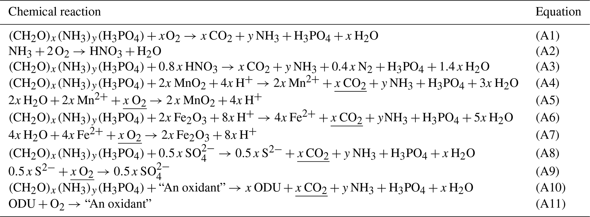
The approach used to describe the anaerobic degradation by MnO₂, Fe₂O₃ and SO₄ as oxidants is based on the equations summarized in Table A1. These anaerobic respiration processes produce reduced substances (i.e., Mn²⁺, Fe³⁺ and H₂S; Table A1, Eqs. A4, A6 and A8). Complete reoxidation of these reduced substances, formed through the oxidation of x moles of C, requires x moles of O₂, regardless of the anoxic pathway considered (Table A1, Eqs. A5, A7 and A9). Hence, as proposed by Soetaert et al. (1996) for the modelling of sediment diagenesis, instead of modeling each of these processes separately, they are lumped together into one process (Table A1, Eqs. A10 and A11), where degradation is only C limited (the quantity of oxidants is assumed non-limiting) and inhibited by O₂ and NOs (Table A1, Eq. 64). All the reduced substances formed by anoxic mineralisation are lumped into one state variable ODU (i.e. Oxygen Demand Unit) with $\mathrm{ODU}=\mathrm{0.5}{\mathrm{H}}_{\mathrm{2}}\mathrm{S}+\mathrm{2}{\mathrm{Mn}}^{\mathrm{2}+}+\mathrm{4}{\mathrm{Fe}}^{\mathrm{2}+}$. The terminal electron acceptors are not explicitly modeled; only the production of reduced substances is described. Anoxic mineralisation of 1 mol of C produces 1 mol of ODU and reoxidation of 1 mol of ODU requires 1 mol of O₂ (Table 1, Eqs. A10 and A11).

Table A1 Idealized reactions representing the degradation of organic matter using different oxidants. The equations describe successively the aerobic organic matter mineralisation (Eq. A1), nitrification (Eq. A2), denitrification (Eq. A3), and anoxic mineralisation via manganese, iron and sulfate reduction (Eqs. A4, A6 and A8, respectively). These three degradation pathways produce the same amount of CO₂ and the oxidation of the reduced substances they produced (respectively, 2 Mn²⁺, 4 Fe²⁺, 0.5 S²⁻) consume the same amount of O₂ (Eqs. A5, A7 and A9, resp.). They are lumped in the model into Eqs. (A10) and (A11) where ODU is the Oxygen Demand Unit ($\mathrm{ODU}=\mathrm{0.5}{\mathrm{H}}_{\mathrm{2}}\mathrm{S}+\mathrm{2}{\mathrm{Mn}}^{\mathrm{2}+}+\mathrm{4}{\mathrm{Fe}}^{\mathrm{2}+}$). y denotes the molar N:P ratio, x the molar C:P ratio in organic matter per mole of phosphorus (for Redfield Stoichiometry, x=106, y=16).