Enabling fast greenhouse gas emissions inference from satellites with GATES: a Graph-Neural-Network Atmospheric Transport Emulation System

Atmospheric observation-based “inverse” greenhouse gas flux estimates are increasingly important to evaluate national inventories. A dramatic improvement in “top-down” flux inference is expected in the coming years due to the rapidly growing number of measurements from space. However, many well-established inverse modelling techniques face significant computational challenges scaling to modern satellite datasets, particularly those that rely on Lagrangian Particle Dispersion Models (LPDM) to simulate atmospheric transport. Here, we introduce GATES (Graph-Neural-Network Atmospheric Transport Emulation System), a data-driven LPDM emulator which outputs source-receptor relationships (“footprints”) using only meteorology and surface data as inputs, approximately 1000× times faster than an LPDM. We demonstrate GATES's skill in estimating footprints over South America and integrate it into an emissions estimation pipeline, evaluating Brazil's methane emissions using GOSAT (Greenhouse Gases Observing SATellite) observations for 2016 and 2018 and finding emissions that are consistent in space and time with the physics-driven estimate. This work highlights the potential of machine learning-based emulators like GATES to overcome a key bottleneck in large-scale, satellite-based inverse modeling, accelerating greenhouse gas emissions estimation and enabling timely, improved evaluations of national GHG inventories.

1 Introduction

Reducing greenhouse gas (GHG) emissions is essential for mitigating climate change, with carbon dioxide (CO₂) and methane (CH₄) being two of the most significant contributors. International agreements such as the Global Methane Pledge, with over 150 participating countries, reflect the commitment to address this challenge, by aiming for a 30 % reduction in emissions by 2030, compared to 2020 levels (European Commission and United States of America, 2021). However, significant uncertainties persist in the inventory-based (“bottom-up”) reports of national methane emissions, which will be used to evaluate progress (Saunois et al., 2020, 2025). “Top-down” or “inverse” estimates of GHG emissions can be used to evaluate and improve these self-reported national emissions inventories and are therefore seen as a valuable tool for supporting international climate agreements (e.g., Leip et al., 2018). These methods use atmospheric concentration observations to quantify surface fluxes, with atmospheric chemical transport models providing the link between these two quantities.

Until recently, top-down studies primarily relied on in situ atmospheric observations from individual stations or networks (e.g., Bergamaschi et al., 2018). Increasingly, CH₄ and CO₂ flux estimates are being derived using satellite data, reflecting the expansion of space-based instruments (e.g., Ganesan et al., 2017; Scarpelli et al., 2022; Tunnicliffe et al., 2020; Western et al., 2021; Worden et al., 2023) , which can provide valuable insights into regions previously under-sampled by in situ data. National emissions estimates have been derived using data from instruments such as GOSAT (Greenhouse gases Observing SATellite , launched 2009; Parker et al., 2020) using regional (Ganesan et al., 2017; Tunnicliffe et al., 2020; Western et al., 2021) or global (Alexe et al., 2015; Feng et al., 2023; Maasakkers et al., 2019) chemical transport models. Current global instruments, like TROPOMI (Tropospheric Monitoring Instrument, launched 2017; Veefkind et al., 2012) have over 100 times the observation density of GOSAT, and recently launched and upcoming satellites (e.g. CO2M, MethaneSAT) will continue to grow the volume of available observations (Jacob et al., 2022). Higher data density increases the spatial and temporal resolution at which fluxes can be inferred, providing the opportunity to better understand the processes driving observed changes in global atmospheric CO₂ and CH₄ abundance.

This rapid growth in data volume, from in situ-based datasets (∼ 1000s of observations per month in a continental region) to satellite-based (∼ 10 000s to 100 000s of observations per month in a continental region), is leading to scaling issues for many traditional approaches to flux inference. One of the most common families of top-down methods for national scale emissions estimation employs Lagrangian Particle Dispersion Models (LPDMs), which use archived meteorological data to simulate the movement of hypothetical gas particles backwards in time from a location to the surface in the surrounding region. The advantage of using LPDMs for GHG flux inference is that LPDMs directly calculate the sensitivity, or “footprint” (Fig. 1a), of a mole fraction measurement to upwind fluxes. This contrasts with Eulerian models, which simulate concentrations in a 3D atmospheric grid rather than using individual particles, and do not directly calculate source–receptor relationships. To be useful in top-down inference, Eulerian model outputs require additional processing to derive sensitivities of observations to fluxes, such as performing ensembles of perturbed flux runs (e.g., Baker, 2006a; Bousquet, 2000; Peters et al., 2005) or deriving adjoint model code (e.g., Baker, 2006b; Kaminski et al., 1999). However, a major disadvantage of LPDMs is that they require one run for each observation (several core-minutes, depending on set-up), leading to high computational burdens for large datasets. Studies show that increasing the number of simulated particles and extending their simulation time reduces statistical errors in the transport model, but these improvements also come at the expense of even greater resource demands (Pisso et al., 2019; Vojta et al., 2022). Although LPDMs are easily parallelizable with high performance clusters allowing for multiple simulations to run simultaneously, the overall computational cost remains substantial and will likely be a barrier in the use of LPDM-based methods for applications involving planned space-based GHG measurements.

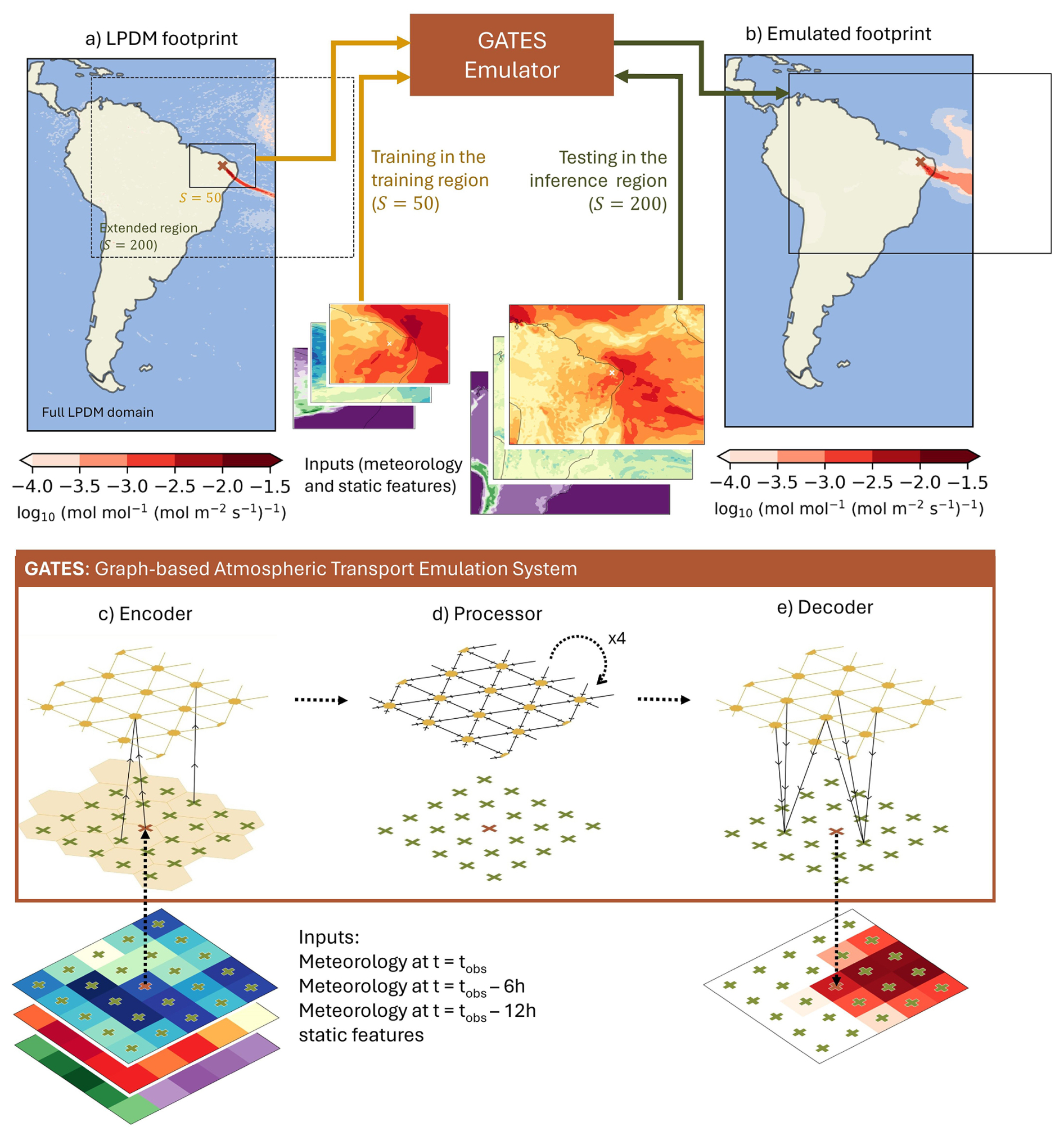
Figure 1 GATES model schematic and architecture. Top: (a) Example of an LPDM-generated footprint (∼ 20 min to generate on a single CPU) showing the sensitivity of a satellite measurement to fluxes from the surrounding domain. (b) Corresponding GATES-emulated footprint (∼ 1.5 s to generate). Both (a) and (b) are shown over the full LPDM domain and resolution (0.352° × 0.234°, ≈ 33 km × 25 km in mid-latitudes) used in Tunnicliffe et al. (2020). In (a), the solid-line box corresponds to the training region, a square of size 50 × 50 grid-cells centered around the coordinates of the satellite measurement. The solid-line box in (b) corresponds to the inference region, a 200 × 200 grid-cell square over which footprints were emulated. When this area escapes the original footprint domain, as above, the added space is filled with zeros and ignored in evaluation (here shown as whitespace inside the boxes). Bottom: Architecture of the graph and emulator, demonstrated for a square domain of size 5 × 5. GATES is composed of (c) an encoder, (d) a processor, and (e) a decoder. The black solid arrows indicate the flow of information. The inputs are represented as node attributes on a latitude–longitude grid (crosses) centered around the measurement point (red cross). (c) In the encoder, local regions of the inputs are mapped into nodes in the abstract feature space (yellow hexagons), arranged as an triangular mesh. Each mesh-node is connected with edges to its six neighbors (yellow lines). (d) In the processor, each mesh-node is updated using message-passing from the neighboring nodes. Four independent message-passing blocks are learned. (e) The decoder maps the latent space back to the original latitude–longitude grid of the same resolution as the inputs, outputting the footprint value at each node.

The satellite community has recognized computational capacity as a key limitation in applying greenhouse gas measurements and inverse modelling to support policy (Joint CEOS-CGMS Working Group on Climate – Greenhouse Gas Task Team., 2024). Two recent studies that use Lagrangian methods for TROPOMI observations over Alaska and Siberia propose methods to coarsen (Thompson et al., 2025) or subsample (Ward et al., 2025) the dense observational dataset, so that it is feasible to run LPDMs. Several recent studies have proposed methods for interpolating or emulating footprints (see below) but none have addressed the challenging problem of emulating satellite footprints at continental scales. In this study, we present GATES (Graph-Neural-Network Atmospheric Transport Emulation System), a new method for footprint emulation that addresses previous limitations, offering high computational efficiency for satellite data whilst retaining sufficient accuracy over large scales for regional flux inference. Section 2 provides background on LPDMs and previous emulation approaches, and Sect. 3 presents the architecture of the machine learning model. In Sect. 4 we describe the generation of LPDM footprints in our case study region, South America, and detail the inputs, dataset and training approach. In Sect. 5 we show and evaluate the outputs of GATES, and most importantly we demonstrate its application in a previously studied top-down inference pipeline to estimate Brazil's methane emissions.

2 Background and problem statement

2.1 Lagrangian particle dispersion models

To calculate the sensitivity of a mole fraction measurement to surface fluxes using LPDMs, thousands of virtual particles are released from a set of 3D coordinates (latitude, longitude, height) and transported backwards in time for a number of days. The model records whenever these particles are near the surface (within 40 m in the simulations used here) throughout the whole time period, creating an aggregated 2D “influence footprint” for each observation that indicates the contribution of a unit surface flux at a particular location to the observed mole fraction. When applied to in situ measurements, the LPDM is initialized using the site coordinates and the inlet height. Satellites, on the other hand, take column-averaged measurements of GHG mole fractions, so instead, a number of 3D releases are run from different heights in the atmosphere, and then averaged using a kernel (e.g. Ganesan et al., 2017). This means that LPDM runs for satellite footprints are more computationally expensive than for in-situ footprints.

Here, we emulate the UK Met Office LPDM NAME (Numerical Atmospheric-dispersion Modelling Environment; Jones et al., 2007), with a similar setup to those used by Tunnicliffe et al. (2020) and Ganesan et al. (2017), who run NAME for valid GOSAT observations to infer methane emissions. They perform NAME simulations for 20 vertical levels, releasing 1000 particles per hour for levels 1–8 and at 100 per hour for levels 8–17. NAME cannot emulate dispersion for the upper three column levels (18–20) and therefore the prior column mole fractions are used. The particles are simulated travelling backwards in time for 30 d from the location and time of each satellite measurement, recording interactions with the surface whenever they are below 40 m above ground level. The calculated sensitivity maps for each vertical level, output at a resolution of 0.352° × 0.234°, are height-averaged into a single 2D footprint, weighted by the corresponding GOSAT averaging kernel and pressure weight. See Ganesan et al. (2017) for more details on the set-up. Other examples of well-known LPDMs that have been applied to similar applications are the FLEXible PARTicle Dispersion Model (FLEXPART; Pisso et al., 2019), the Hybrid Single-Particle Lagrangian Integrated Trajectory model (HYSPLIT; Stein et al., 2015) and the Stochastic Time-Inverted Lagrangian Transport Model (STILT; Fasoli et al., 2018).

2.2 Meteorology

LPDMs are usually driven by a meteorological reanalysis product. Here, our NAME simulations use the Met Office Unified Model (UM) global analysis fields to simulate particle dispersion. The global model has a resolution of 3 h and 25 km up to July 2014, 17 km from then until July 2017 and 12 km thereafter, with 59 vertical levels up to 29 km (Met Office, 2025a, b). NAME also uses static fields (i.e. not time dependent) of surface characteristics, including orography, a sea-land mask, and a land surface type map with nine categories (including different types of trees and grasslands, urban, bare soil and ice; Essery et al., 2001), at a resolution of 0.156° × 0.234°.

2.3 Problem statement

Summarised mathematically, an LPDM f produces a footprint $y_t^{\mathit{\phi }}$ by modelling backwards particle dispersion from a set of coordinates φ at time t. For this, it uses static information ω including topography and land-use maps, and a time series of 3D meteorological features, starting at time t (x^t) and extending backwards in time from t for a number of steps N with separation Δt. The meteorological input time series can therefore be defined as $x^{t:t-N\mathrm{\Delta }t}=[x^t,x^{t-\mathrm{\Delta }t},\mathrm{\dots },x^{t-N\mathrm{\Delta }t}]$, and the LPDM summarized as $y_t^{\mathit{\phi }}=f(\mathit{\phi },x^{t:t-N\mathrm{\Delta }t},\mathit{\omega })$. The LPDM setup described here uses Δt = 3 h, and N=240, which equates up to tracking particles backwards in time for 30 d.

Our goal is to develop an efficient emulator Φ that can accurately recreate footprints produced by the LPDM in orders of magnitude less time and potentially using only a subset of the full LPDM inputs. Thus, the emulator predicts a footprint as ${\widehat{y}}_t^{\mathit{\phi }}=\mathrm{\Phi }(\mathit{\phi },\stackrel{\mathrm{̃}}{x},\stackrel{\mathrm{̃}}{\mathit{\omega }})$ where $\stackrel{\mathrm{̃}}{x}\subseteq x^{t:t-N\mathrm{\Delta }t}$ and $\stackrel{\mathrm{̃}}{\mathit{\omega }}\subseteq \mathit{\omega }$.

2.4 Previous ML approaches

The urgent need for scalable LPDM-based inverse methods was previously addressed by Roten et al. (2021), Fasoli et al. (2018), Cartwright et al. (2023) and others, who derived modest gains in computational efficiency through interpolation-based approaches. More complex machine learning (ML) methods such as those developed by Fillola et al. (2023) and He et al. (2025) introduced proof-of-concept emulators of LPDM footprints for surface sites using meteorological fields as inputs. One of these studies (Fillola et al., 2023) used a set of individual regressors to emulate the footprint value at each grid-cell for in-situ observation towers, but only estimated these values for part of the footprint, within ∼ 100 km of the measurement site. Therefore, to perform flux inversions, the emulated footprints had to be nested within a low-resolution LPDM simulation. The emulator developed in He et al. (2025) focuses on emulating high-resolution in-situ footprints (400 km × 400 km domain at 1 km resolution) for an urban sensor network (Dadheech et al., 2025). To constrain their convolutional neural network architecture, one of the key inputs was a Gaussian plume, a simplified footprint approximation calculated using the meteorology at the measurement site. While this approach is effective for local-scale dispersion, it is unlikely to be suitable for national or continental transport (∼ 1000–5000 km) because the assumptions underpinning the Gaussian plume model (such as constant wind speed and homogeneous atmospheric conditions) only hold over ∼ 10 km spatial scales.

3 Model architecture

The Graph-Neural-Network Atmospheric Transport Emulation System (GATES) is a ML-driven emulator of regional LPDM-derived satellite observation footprints using meteorological and topographical inputs. The architecture of GATES builds on that of Keisler (2022) and Deepmind's Graphcast (Lam et al., 2023), who developed weather forecasting models using Graph Neural Networks (GNNs) with an encoder–processor–decoder structure. This architecture achieved breakthroughs in deterministic weather forecasting, sometimes outperforming the reference physical models (Lam et al., 2023), as well as effectively learning complex systems based on Partial Differential Equations (PDEs), like fluid dynamics and diffusion (Pfaff et al., 2020; Sanchez-Gonzalez et al., 2020). Many of these systems are designed to learn a one-step forward model, predicting system quantities at time t+1 given the current state (and often previous states too). Unlike these previous studies, GATES is trained to return time-integrated 2D GHG measurement footprints without requiring information about the intermediate model timesteps.

As inputs, GATES takes a subset of the meteorology that drives the LPDM, reducing input/output overhead and memory requirements compared to running the LPDM: we provide a number of snapshots of the state of the atmosphere at the time of the satellite measurement and before, including variables like wind direction, wind speed and planetary boundary layer height, as a latitude–longitude grid and at selected vertical levels. These inputs are complemented with time-independent variables, including the latitude–longitude coordinates of each grid-cell, its distance from the measurement, the surface height above sea level, and the main landcover type.

Graph Neural Networks represent data as a graph, composed of nodes and connecting edges. In GATES, each coordinate in the latitude–longitude grid is treated as a node, with the inputs at that location considered its attributes. The encoder-processor-decoder architecture means that the inputs on a latitude–longitude grid are first translated (“encoded”) into an abstract space, “processed” iteratively to spread the information, and then “decoded” back into the original latitude–longitude grid, making predictions for the footprint value at each grid-cell. Figure 1 shows a schematic of the architecture of GATES. In the encoder (Fig. 1c), the input grid is encoded in a lower-resolution regular triangular mesh, which acts as an internal abstract feature space. This mesh, built with the h3 library (Uber Technologies Inc, 2024), divides the domain into hexagons with an average area of 1770 km², and with mesh nodes placed ∼ 40 km from each other. We place edges between each node in the lat-lon grid and its closest node in the mesh, so that each mesh node receives a Multi-Layer Perceptron (MLP) encoding of the distance-weighted mean of the local features. MLPs are simple feedforward neural networks composed of multiple layers of linear transformations and non-linear transformation functions, which here are used to update node and edge features based on local information. In the processor (Fig. 1d), each node in the mesh is connected to its six adjacent nodes, and the whole mesh is updated in multiple message-passing rounds. Each message-passing GNN block (Battaglia et al., 2018) first uses an MLP to update the features of the edges in the mesh using information from the adjacent nodes, and then another MLP to update each node based on its adjacent features. In the decoder (Fig. 1g), a final MLP maps the mesh-node features back to the original latitude–longitude grid, outputting the footprint (Fig. 1e).

GATES is inherently flexible because it operates through local, node-wise computations. At every stage (encoding, processing, and decoding) the model learns to update each node based only on its neighbours' features, rather than relying on a regular grid or fixed input dimensions. Traditional architectures such as Convolutional Neural Networks (CNNs), on the other hand, require inputs to be defined on uniform, fixed-sized grids, where emulation depends on the resolution and dimensions of the training domain. With GATES, training and inference can be done at different resolutions, geometries or domain sizes, without needing to retrain or modify the architecture.

4 GATES in practice: emulating GOSAT footprints over South America

To demonstrate the model, we train GATES to emulate NAME footprints for GOSAT observations over South America, as presented in Tunnicliffe et al. (2020). Tunnicliffe et al. produce NAME footprints for GOSAT observations that pass the quality threshold over an area defined by 35.8° S to 7.3° N and from 76.0 to 32.8° W. They produced observation for both nadir measurements (over the land) and glint measurements (over the ocean), but, in Tunnicliffe et al., they use only nadir measurements within the inversions to avoid any biases between the two. GATES is trained and validated using data from 2014 to 2016, both over the land and the ocean, and emissions are derived for 2016 and 2018, using only land-based measurements following the reference study. The year 2018 was chosen to demonstrate the performance of the GATES-based inversion as it is separated in time from the data used in the training and validation set. The footprints aggregate the surface interactions of particles transported for the 30 d leading up to the satellite measurement at a resolution of 0.352° longitude × 0.234° latitude (≈ 33 km × 25 km in mid latitudes), constrained to a domain that covers the whole South American continent (60.98° S to 22.32° N and 91.33 to 24.8° W with a grid of size 190 × 357). Each footprint takes about ∼ 20 core-minutes to be generated on a high-performance cluster.

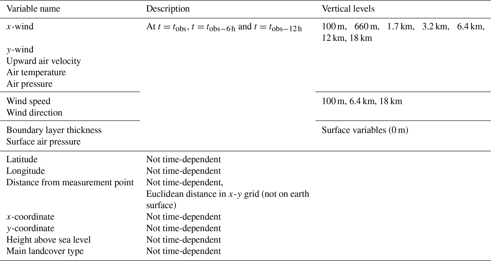
Table 1 Input variables provided to the emulator. In total, there are (2 atmospheric surface variables + 7 atmospheric variables × 7 levels) × 3 timesteps + 2 topography variables + 5 constant variables = 160 input features.

4.1 Inputs: meteorology and topography

This version of the emulator takes as main inputs nine physical variables at seven vertical levels in the atmosphere (see Table 1 for all the variables and levels used). The meteorology is interpolated linearly from its 3-hourly resolution t, as well as any required previous timesteps up to $t-\stackrel{\mathrm{̃}}{N}\stackrel{\mathrm{̃}}{\mathrm{\Delta }t}$. In the application described here, $\stackrel{\mathrm{̃}}{N}=\mathrm{2}$ and $\stackrel{\mathrm{̃}}{\mathrm{\Delta }t}$ = 6 h, so that the meteorological input to each footprint is composed of the weather state at t, 6 and 12 h before. This is a small subset of the full NAME input meteorology, which usually requires ∼ 15 meteorological variables at 50 atmospheric levels at over 200 timesteps. We also provide the model with information from the static fields NAME uses to describe topography (orography and landcover type), as well as two variables with the x- and y-coordinates of each grid-cell with respect to the measurement coordinates (so that the grid-cell with the satellite observation is [0,0]) and a variable with the Euclidean distance from each grid-cell to the measurement coordinates. Each input is a 2D field of the same resolution and domain as the corresponding footprint. The vertical levels and the number of timesteps were decided through tuning, where a small range of hand-crafted configurations were tested.

4.2 Preparing the dataset

GATES is designed to be LPDM domain agnostic: instead of emulating footprints over the whole LPDM domain, which tends to be sparse, GATES emulates footprints on a square domain of S×S grid cells centred around the measurement coordinates φ. The meteorology and static fields are cropped to the same area for each corresponding footprint.

For this South America application, GATES is first trained on a square (in latitude/longitude space) of size S = 50 grid cells centered around the satellite measurement. Subsequently, footprints are emulated over a square of S = 200 grid-cells (∼ 6000 km × 5000 km; see the training and inference regions in Fig. 1a and b). We find that training in the smaller domain is not only more computationally efficient, but that the model performs better than training on the S = 200 domain, likely because the wider domain is mostly sparse. We choose to define our inference region as S = 200 as our preliminary tests suggest this size of domain doesn't introduce substantial error in the simulated mole fractions, compared to simulations using a larger region. When using the emulated footprints in the inference emissions pipeline, we fill the rest of the full LPDM domain with zeros.

We split our dataset into training, validation, and test sets using distinct time periods, to imitate deployment conditions and to avoid the high autocorrelations in meteorological fields from polluting the evaluation results. We use the first 2 years to train the model (2014–2015, 11 165 samples), validate on January, February and March of 2016 (4314 footprints), and evaluate the outputs for the remaining months of 2016, as well as the whole of 2018 (36 671 footprints, 16 945 from 2016 and 15 412 from 2018). The validation set was used to tune model hyperparameters, and to calibrate the bias correction. Figure A1 shows the spatial and seasonal distribution of the datasets used.

4.3 Training details

4.3.1 Data normalization

During training, the non-zero values in the footprints are log-transformed and shifted by the minimum value in the training dataset, so that all non-zero values in the original footprints y remain strictly positive in the transformed footprints y^′. The zero values are maintained as such. This helps tackle the footprints' strong exponential distributions, with values decaying quickly with distance from the measurement point. The emulated footprints on the test set are returned to the original space for evaluation. All inputs are standardized (zero mean and unit variance). Each atmospheric variable is standardized per atmospheric level (where relevant) and across all different input timesteps.

4.3.2 Model parameters

All neural networks in the GNN are MLPs with two hidden layers of size 16 and an output layer size of 64, except the decoder MLP, which has only one hidden layer and an output size of 1 (as a single value is predicted at each node). Here, size refers to the number of neurons in each layer. The size of the layers and the number of the hidden layers was decided through tuning, testing a number of configurations. Deeper networks or with higher number of nodes led to the model over-fitting to the training data, whereas shallower networks achieved low skill as they were unable to learn complex dispersion patterns. All MLPs use Relu (Nair and Hinton, 2010) as the activation function and are followed by a LayerNorm (Ba et al., 2016) layer (except the decoder's MLP, which outputs the footprint value).

4.3.3 Loss function

The loss function L weights mean squared error (MSE) by the footprint value, which applies stronger penalties for mispredicting areas with higher relevance. It first calculates the pixel-by-pixel squared error between the predictions and the true footprints (both in the transformed space, i.e. $\widehat{y^{\prime }}$ and y^′, respectively), and then weights it by a linear transformation g() of the original footprint y, before taking the mean across the footprint. For each batch, we average the loss from all the footprints uniformly.

$$L=l\left(\widehat{y^{\prime }},y^{\prime }\right)={\displaystyle \frac{\mathrm{1}}{S^{\mathrm{2}}}}\sum _{\mathbf{i}=\mathrm{1}}^S\sum _{j=\mathrm{1}}^{S}g\left(y\right(i,j\left)\right)\times {\left(\widehat{y^{\prime }}(i,j)-y^{\prime }(i,j)\right)}^{\mathrm{2}}$$

where

$$g\left(y\right)=wy+a$$

Here, we use w=1000 and a=0.5. This training objective was minimized with the ADAMW (Lam et al., 2023; Loshchilov and Hutter, 2019) optimizer and a learning rate of 5 × 10⁻⁵, which controls the size of the parameter updates during optimization. We use a batch size of 5, which determines how many samples get processed together in each update during training, regularising the learning.

4.4 Thresholding and bias correcting the footprints

ML regression tasks, which predict continuous values, often struggle to predict exactly zero, predicting instead very small values. The footprints, however, are sparse, with large regions of areas with no sensitivity (i.e. zeros). Therefore, following inference, the near-zero background values below a calculated threshold are set to zero, imitating approaches from precipitation modelling (Schmidli et al., 2006). The footprints are also bias-corrected by applying quantile mapping (Met Office, 2018). This bias correction is necessary to avoid the model's tendency to underpredict, likely caused by the sparsity of the outputs. The calibration of the threshold and the quantile mapping are both done using the validation set, transformed back to the original data space. GATES is not retrained after thresholding and bias correction: these two statistical steps are applied as post-processing of the already emulated footprints. Figure B1 illustrates the steps for a particular footprint.

4.4.1 Output thresholding

A “footprint threshold” is defined on the validation set such that the threshold exceedance frequency across all the grid-cells in the emulated footprints matches the above-zero frequency in the LPDM-generated footprints (Schmidli et al., 2006), so that there is the same number of non-zero values in both validation datasets. The threshold is calculated to be 1.76 × 10⁻⁵, which is consistent with just removing small background values. In the test dataset, all values under this threshold are set to zero.

4.4.2 Bias correction

After thresholding, the distribution is corrected using quantile mapping. This technique maps the cumulative distribution function (CDF) of the emulated data to that of the true data, applying a transformation function T(x). We define T(x) by dividing the CDF of the true data in the validation set in 5000 quantiles, and the CDF of the emulated data into the same number of quantiles, and mapping the two. After T(x) has been defined on the validation set, it is applied to the test set. Figure B2 shows the CDF of the footprint values in the test set before and after the transformation, with an improved fit and reduced bias.

4.5 Hardware and time requirements

We train and run the model on a 32 GB NVIDIA V100 GPU. It takes 10 h to fully train, including loading all the data and model into memory. For emulation, each footprint takes around 1 s to produce on the same V100 GPU (after an initial overhead to load the model and the input data), whereas a single footprint LPDM footprint takes ∼ 20 min. GATES can therefore generate footprints 1000× faster than the physics-based simulation.

Integrating the emulator in the emissions inference pipeline presents a significant speed-up. Generating footprints for a regional monthly inversion as shown here (∼ 1000 footprints) would take ∼ 20 min with GATES, but 14 core-days with the LPDM.The inversion algorithm itself, described in Sect. 5.3, combines the observations, footprints and prior emissions to output updated emission fluxes takes 6–10 h on a CPU, depending on the number of data points assimilated. We use a computationally expensive hierarchical Bayesian Markov Chain Monte Carlo inverse method, as outlined in Ganesan et al. (2014).

GATES therefore shifts the primary computational bottleneck to the inversion algorithm, which now dominates the runtime. Substantially higher overall inversion speed-ups would be obtained if a less expensive inverse method was used. As noted in Dadheech et al. (2025), the use of an efficient emulator has the added potential advantage that footprints do not need to be archived and can instead be produced on demand, substantially reducing storage requirements. Further speed-up to GATES is expected with software optimization in the future.

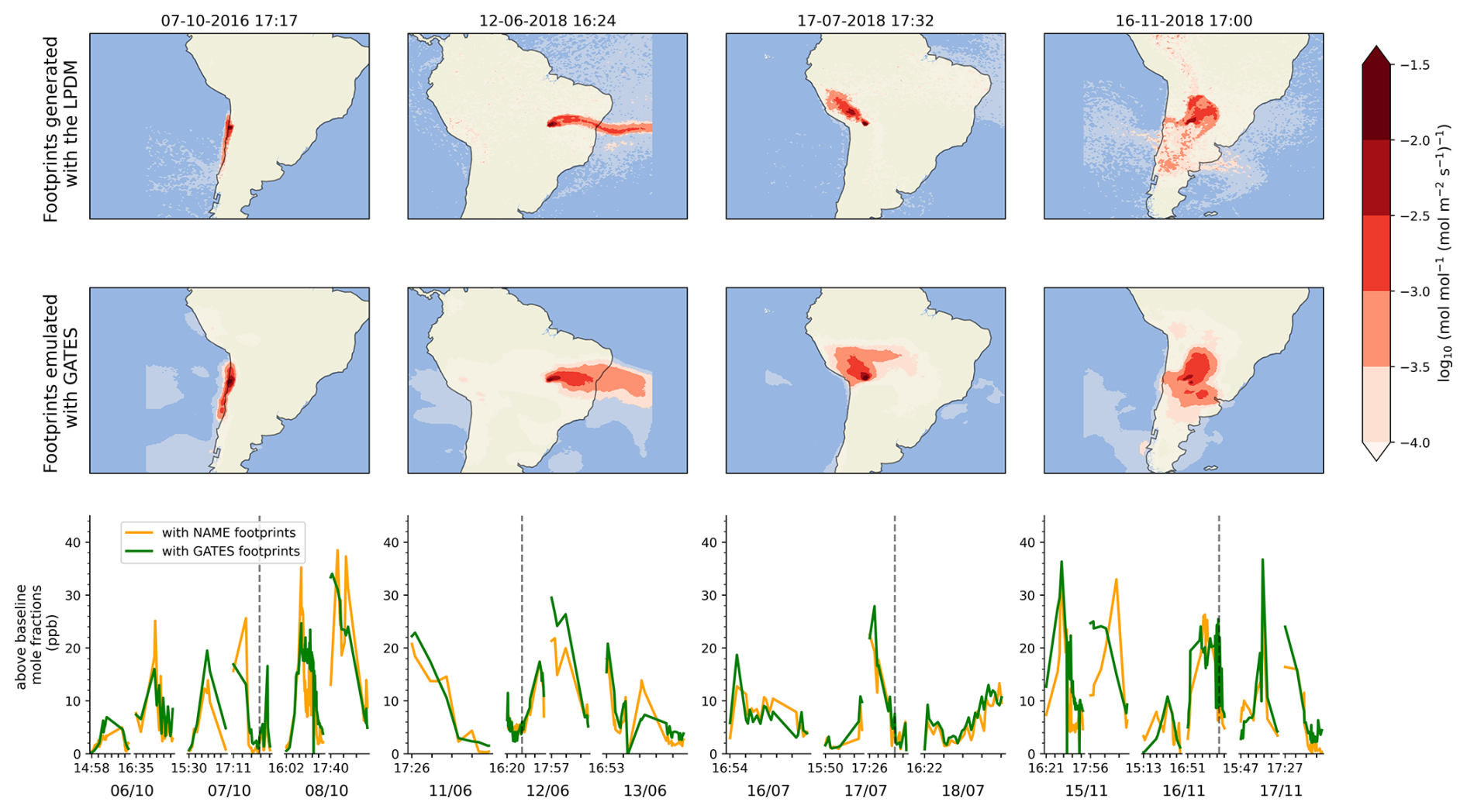
Figure 2 Example GATES outputs. Four LPDM-generated footprints from the test dataset (top row) and their GATES-emulated counterparts (second row). The bottom row shows modelled above-baseline mole fractions, derived with the LPDM footprints (orange) and the GATES footprints (green). Each box shows the timeseries for three days with breaks between days indicated by wider gaps between the lines. Each tick mark corresponds to two minute intervals. For days where the satellite scans the continent multiple times, we indicate the time of the first measurement of each overpass. The dashed line indicates the date and time of the footprints shown in the corresponding top two rows. Mole fractions are calculated by convolving each footprint with a prior, producing the estimated methane contribution in ppb from each grid cell to that particular measurement, and summing over the domain to calculate the total expected contribution from local sources (i.e. above the background baseline).

5 Evaluating GATES performance: footprints, predicted concentrations and inferred emissions

In this section we use a range of tests to evaluate the performance of the emulated footprints at three stages of the inversion pipeline: (1) metrics to compare the emulated footprints to the LPDM, (2) comparison of simulated methane column mole fractions over South America, and (3) comparison of Brazil's inferred methane emissions at monthly resolution for April–December 2016 and all of 2018. Figure 2 shows four examples of LPDM footprints and their emulated counterparts, as well as the emulated methane mole fractions for those days. We show that the monthly flux estimates using GATES are comparable to those obtained using LPDM footprints at national and sub-national scales.

The definition of all the metrics used can be found in Appendix C. We evaluate the footprints themselves using the Correlation of Coefficient between the predicted and the true values, both in the original data space and in the logged space. The correlation in the original space captures how well the model reproduces the overall magnitude of the footprints, whereas applying the metric in the logged space gives more weight to low-magnitude values, often more diffuse and challenging to model. To quantify the spatial accuracy of the predicted footprints we use the metric Intersection over Union (IoU), which calculates the overlap between the predicted and true nonzero regions. The timeseries of simulated methane mole fractions is evaluated using standard metrics: the Coefficient of Correlation to assess the agreement between GATES and LPDM mole fractions; the Mean Absolute Error (MAE) and Root Mean Square Error (RMSE) to quantify average and large errors, respectively; and the Mean Bias to indicate any systematic over- or underestimation in the predictions. The monthly emissions calculated with the inversion algorithm are evaluated using MAE and Mean Bias.

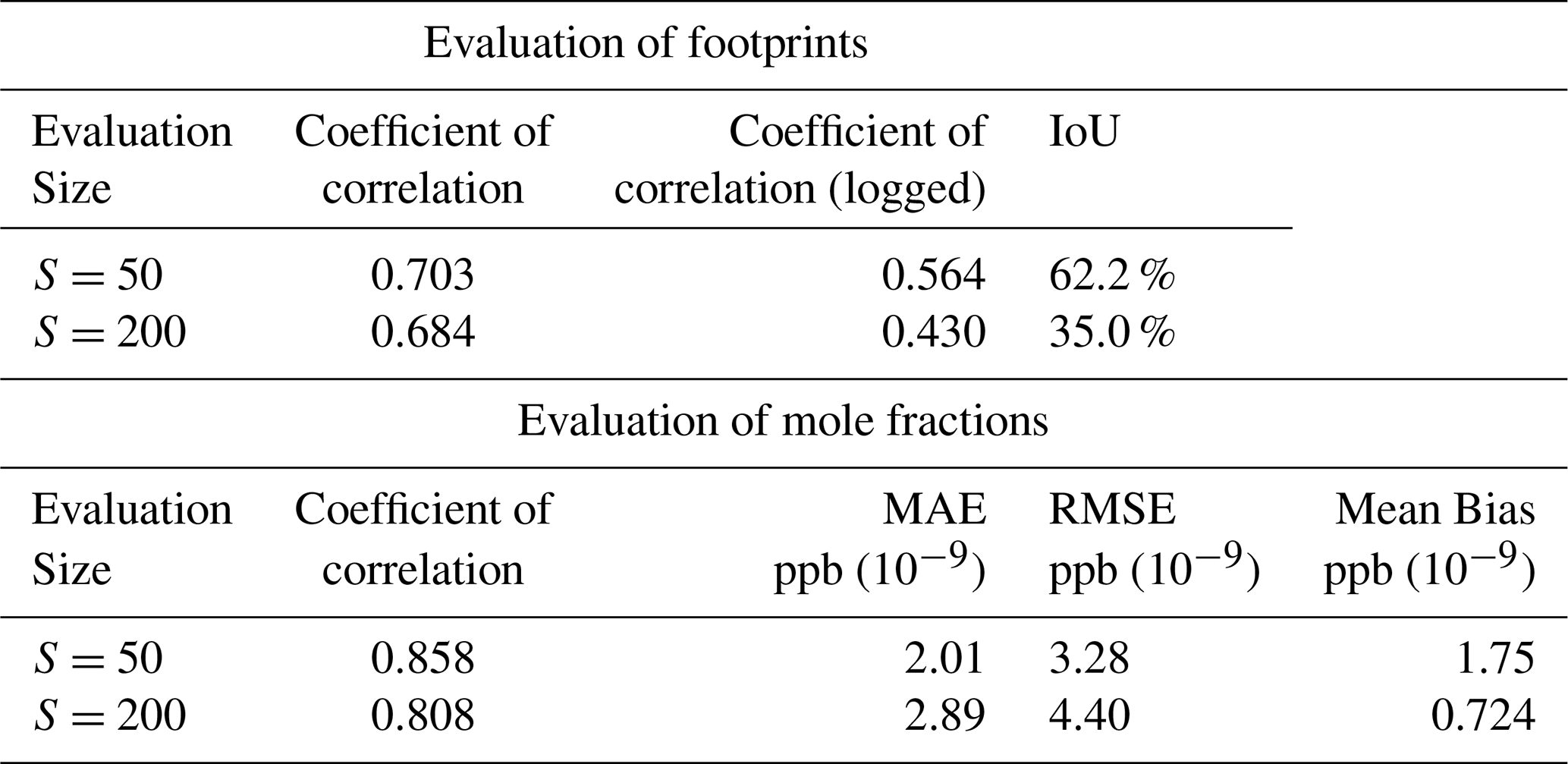
Table 2 Evaluating GATES. Top: comparing footprints against the LPDM outputs. We show the mean score across footprints, averaged for the testing dataset, at the training region (S=50) and the inference region (S=200). Bottom: Evaluation of mole fraction timeseries, averaged across the testing dataset, also shown at the training and inference regions.

5.1 GATES-emulated footprints compared to the LPDM

Example emulated footprints (Fig. 2, middle row) and a set of goodness-of-fit metrics (Table 2) show that GATES captures well the overall shape and magnitude of the LPDM footprints over a range of meteorological regimes and locations in South America. However, the GATES outputs often tend to be somewhat smoother than the LPDM. This is primarily thought to be because the MSE loss function favours averaging in regions of high variability (similar smoothing effects have also been reported when using different architectures with MSE losses in LPDM emulation tasks (He et al., 2025). Moreover, since the LPDM is stochastic, the model outputs exhibit small-scale noise far from the measurement location, which is not reflected in the emulated footprints. However, this noise has little impact on receptor mole fraction predictions. The model's connected architecture may also contribute to the smoothing effect, as similar behavior has been observed in weather applications using a similar machine learning model framework (Lam et al., 2023).

We evaluate the spatial agreement of the emulated footprints using Intersection over Union (IoU) and the accuracy of the predictions using the correlation of coefficient (see Appendix C for all metrics), averaging both scores across all footprints in the test dataset. In the near-field (training region, S = 50, Box A in Fig. 1), GATES achieves a mean IoU score (± 1 standard deviation) of 62 % ± 23 % and a mean correlation of coefficient of 0.70 ± 0.13. Emulating the far field (full emulation domain, S = 200, Box B in Fig. 1) is a more difficult task, as the particles have travelled further from the measurement point and from each other. It is also a prediction area unseen to GATES during training. There is an expected drop in performance, particularly in the IoU as the LPDM footprints become noisier (IoU of 35 % ± 12 %, correlation coefficient to 0.68 ± 0.13). The drop in the correlation of coefficient is smaller as it is dominated by the large values very close to the measurement point.

We find that model performance is generally poorer in regions with more heterogeneous topography (see Fig. D1), with footprints near the Andes scoring lower across all metrics. Chemical transport models are known to struggle over complex terrains (Brioude et al., 2012), potentially leading to more variance in the outputs and more difficult footprints to emulate. In addition, the seasonal and spatial distribution of observations in the training data might also influence performance: there are fewer training footprints in some of the mountainous areas, which could limit the learning. In contrast, the July–August–September season consistently achieves better metric scores, likely due to a higher number of available training samples, or potentially because the meteorology in this season is easier to capture (Fig. 1).

5.2 Evaluating simulated mole fractions

In the inversion pipeline, each footprint is convolved with an emissions field (element-wise multiplication of both 2D fields and then summation over the whole area) to calculate the modelled atmospheric column-averaged mole fraction at the satellite observation location and time. Here, we convolve both sets of footprints (emulated and LPDM-derived) with the emissions field from Tunnicliffe et al. (2020), which includes anthropogenic (EDGAR (Emission Database for Global Atmospheric Research) v4.3.2 database; Janssens-Maenhout et al., 2019), biomass burning (GFED (Global Fire Emissions Database) v4.1) and wetland (SWAMPS (Surface WAter Microwave Product Series) Schroeder et al., 2015).

Figure 2 (bottom panel) show examples of the timeseries emulated with GATES and the LPDM, for twelve days across the testing dataset. The GATES-modelled measurements achieve a correlation coefficient of 0.81 with the LPDM-modelled data. The Mean Absolute Error (MAE) and Root Mean Squared Error (RMSE), of 2.89 and 4.40 ppb, respectively, are well below the estimated instrument GOSAT repeatability of 13 ppb (Parker et al., 2020). The errors between the two timeseries are approximately normally distributed, with a small tendency for GATES to overpredict (Mean Bias 0.72 ppb). Figure E1 shows the modelled mole fractions in space and seasonally, revealing spatial patterns in the mean bias. The model over-predicts mole fractions in west Amazonia and in the South of Brazil, and underpredicts mole fractions over the North Andes, in Peru and Bolivia. These regions had already been identified as having higher errors the footprint-wise metrics (Fig. D1). 1.6 % of the emulated mole fractions show an absolute error greater than 13 ppb. Figure F1 shows examples of instances where the mole fraction errors are large: These footprints are often near large cities, where the calculated mole fractions themselves are large and where the influence of emulation errors, particularly the above-mentioned smoothing, becomes more pronounced.

5.3 Inversion

Assessing the performance of the emulated footprints in a full methane flux inversion is key to ensuring that GATES is fit-for-purpose. Here, we follow a well-studied previous example, using GOSAT observations over and near Brazil (see Tunnicliffe et al., 2020) and an inversion set-up similar to Western et al. (2021) and Ganesan et al. (2014), who use a hierarchical Bayesian method to estimate monthly regional emissions. Brazil was chosen as a case study, because it is a large country where there are major and diverse CH₄ emissions from human and natural sources, which are not well understood (Tunnicliffe et al., 2020). We carry out this process for two inversion setups that are identical except for the footprints used: one uses the LPDM-generated footprints (those used in Tunnicliffe et al., 2020), the other uses the GATES-emulated footprints.

We use a hierarchical Bayesian Markov Chain Monte Carlo (HB-MCMC) inversion algorithm as described in Ganesan et al. (2014) and used for example by Western et al. (2021) and Ward et al. (2025). This method enables a better characterisation of uncertainty by applying “uncertainties in the uncertainties”. We use the same parameters as Western et al. (2021). In this set-up, the LPDM footprints quantify the contribution of local emissions (i.e. from within the domain) to the modelled methane measurement. The contributions from outside the domain (“background”) must also be quantified. As well as the footprints, NAME outputs sensitivities for each of the boundaries of the domain, which get convolved with concentration “curtains” from the ECMWF CAMS reanalysis database (Inness et al., 2019) to calculate the background concentrations incoming from the edges of the domain. These contributions also get adjusted as part of the inversion. In this work, GATES emulates only the footprints – the boundary sensitivities are used as generated by NAME throughout, to isolate the effect of the emulator.

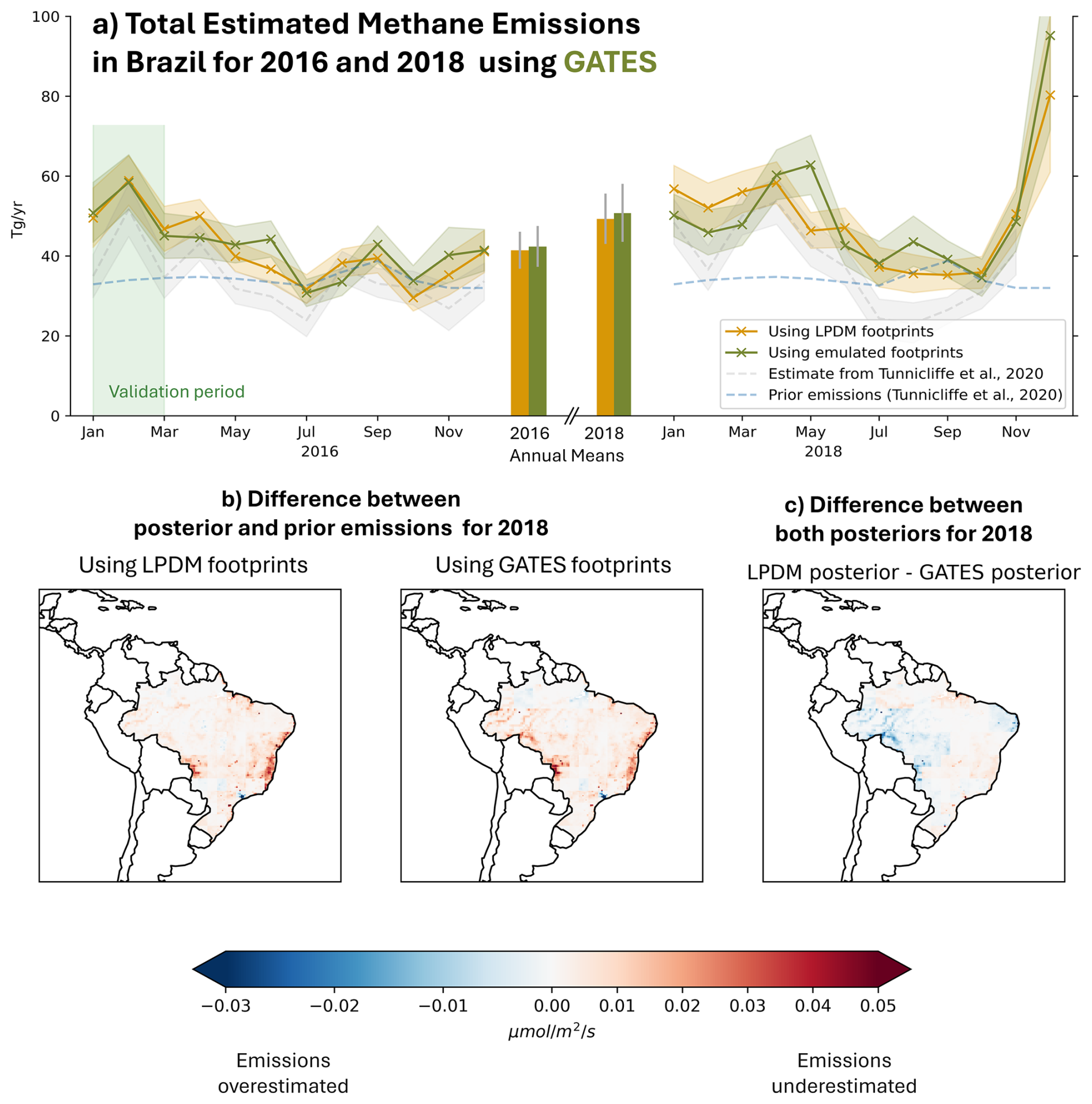
Figure 3 Deriving methane emissions for Brazil, in time (top panel) and space (bottom panels). (a) Estimated methane emissions, for 2016 and 2018. We compare the emissions estimates derived in an inversion using the LPDM footprints (yellow) with those emulated by GATES (green). The emissions inferred with the emulated footprints are well within the posterior inversion uncertainty of the emissions inferred with the traditional method. Note that we report the annual means (bars at the center of the plot) for the full 2016 (i.e. including the validation set January-March) to allow for like-for-like comparisons with 2018. We also show the monthly priors used by Tunnicliffe et al. (2020) and their derived emissions. (b) Difference between the inversion posterior and prior fluxes for 2018, using the LPDM footprints (left) and the GATES footprints (right). The difference highlights the areas that were underestimated or overestimated in the initial estimate. The fluxes calculated with the GATES footprints (right) show good spatial agreement with those calculated from the traditional method (left). (c) Difference between the two posteriors for 2018. Blue shows the areas where the GATES posterior estimates higher emissions than the LPDM posterior, and red shows the opposite.

Table 3 Mean yearly methane emissions for Brazil in 2016 and 2018, estimated using the LPDM footprints and GATES emulated footprints, and mean errors between the two monthly timeseries. We show that the Mean Absolute Error for the monthly timeseries is comparable to the uncertainty in the yearly estimates. Results are displayed for the full 2016 (January–December), the 2016 test set (April–December), the full 2018, and 2018 excluding December. December 2018 has  < 100 valid observations, and therefore the inferred emissions have very high uncertainties which is reflected in the annual mean. This month was also excluded from the analysis conducted by Tunnicliffe et al. (2020).

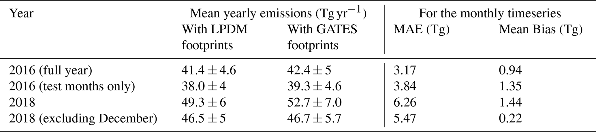
We find that the yearly flux estimates calculated with GATES are in good agreement with the more computationally expensive LPDM-powered estimates: the inversion using the LPDM footprints estimates Brazil's mean yearly emissions of methane to be 41 ± 5 Tg yr⁻¹ for 2016 and 49 ± 6 Tg yr⁻¹ for 2018, and the inversion using the GATES footprints estimates 42 ± 5 and 53 ± 7 Tg yr⁻¹, respectively (see Table 3 for the disaggregated metrics). Figure 3a shows the estimated monthly emissions for Brazil across the two years, where the Mean Absolute Error (only for the test months) is 3.8 Tg yr⁻¹ in 2016 and 6.3 Tg yr⁻¹ in 2018, which is comparable to the posteriori emission uncertainties. Any errors in the GATES emulation will be propagated to the inversion: the GATES-derived emissions are generally higher than the LPDM-derived ones, consistent with footprints being overall underpredicted in the model. There is also a difference in the magnitude of the uncertainties themselves, with the GATES-driven inversion presenting approximately 15 % higher uncertainties in the mean yearly estimates. This additional uncertainty likely reflects the extra error due to the emulation, which is propagated through to the fluxes via our hierarchical Bayesian approach that explores model-data uncertainty as part of the inversion.

Figure 3b shows the difference between the derived emissions (posterior) and the initial estimate (prior) for 2018 for the two inversions, and Fig. 3c shows the difference between these adjustments. The fluxes are generally in good spatial agreement (Mean Absolute Error in the derived fluxes of 0.003 $\mathrm{\mu }\mathrm{mol}{\mathrm{m}}^{-\mathrm{2}}{\mathrm{s}}^{-\mathrm{1}}$ compared to mean value of 0.010 $\mathrm{\mu }\mathrm{mol}{\mathrm{m}}^{-\mathrm{2}}{\mathrm{s}}^{-\mathrm{1}}$ across the two years). Both inversions most notably increased the prior estimate in Brazil's east coast and in the Pantanal region on the border with Bolivia. The GATES posterior shows larger emissions coming from Western Amazonia than the LPDM-driven posterior. This region consistently shows higher errors in the footprint-wise metrics (Fig. D1) and consistent underprediction of the mole fractions (Fig. E1), consistent with deriving higher emissions. Simulated methane concentrations based on the LPDM-derived posterior and the GATES-derived posterior both show a significantly improved fit to the observed GOSAT XCH₄ compared to the prior-based simulations (see Appendix G). The two posteriors show consistent corrections to the prior, with the GATES-based simulations showing only a small positive mean bias of 2.69 ppb relative to those from LPDM.

Overall, our flux estimates for Brazil are consistent within uncertainties with several previous studies that have used GOSAT and inversions based on LPDMs or Eulerian models (Janardanan et al., 2020; Wilson et al., 2021). Whilst within uncertainties, the mean GATES and LPDM estimates are somewhat higher than that of Tunnicliffe et al. (2020). This difference occurs, despite the same satellite observations and LPDM because Tunnicliffe et al. (2020) also incorporated surface data from Ragged Point, Barbados, and used a different inverse method.

6 Discussion and conclusions

We present GATES, a novel ML-driven approach to emulating LPDM footprints using graph neural networks. We demonstrate its use as a stand-alone application, but most importantly within the primary intended workflow, to infer GHG emissions using satellite mole fraction observations. The high consistency of the estimates of Brazil's methane emissions from the ML-enabled pipeline with those based on the physical model, at a fraction of the computational cost (>1000 times faster), demonstrate the potential of this emulator to accelerate greenhouse gas estimations.

One of the main limitations of GATES, as identified for similar GNNs in weather applications (Lam et al., 2023), is that the outputs tend to be smoother than the LPDM footprints. This is likely due to the use of an MSE-based loss function, which encourages less variance in the outputs rather than accurately reproducing fine-scale spatial details, particularly in areas of higher uncertainty. This effect can be observed in Fig. 2, especially in the second footprint, where the predicted plume is in the correct region and direction, but is broader than that of the LPDM. Smoother footprints may lead to higher inference errors in regions of more point-like sources, such as cities or oil and gas infrastructure (see Fig. F1).

Alternative architectures may help to improve future versions of GATES. GATES is a deterministic model, generating a single footprint for a set of inputs, whereas LPDMs are inherently probabilistic. This difference contributes to the smoothing effect, as GATES tends to predict an average outcome rather than generating multiple plausible outputs. Incorporating probability into the emulation would likely produce sharper outputs and contribute to a more rigorous quantification of uncertainty. Understanding uncertainty would also improve explainability, highlighting the areas where the model presents more variance. Further improvements to the architecture of the model could also increase its predicting capabilities, e.g. by integrating multi-meshes like Lam et al. (2023) to capture dispersion at different scales, or adaptive mesh refinement (Pfaff et al., 2020) to encourage higher resolution predictions only around the footprint, or in complex geographies.

Emulating the boundary sensitivities is a key step to fully integrate GATES into an inversion pipeline. These boundary sensitivities are used to calculate the background concentrations, incoming from outside the domain. In this work, we use the boundary sensitivities generated by the LPDM throughout, isolating the effect of the column-averaged footprint emulator. Future work will address this limitation, developing a boundary condition emulator.

Here, we show GATES in application, using GOSAT data to infer emissions from Brazil, but we expect that it could be readily extended to other regions and instruments. As there are only minimal differences in the setup of LPDM simulations for retrievals of similar short-wave infrared satellites, GATES should also be easily re-trainable to several existing and upcoming mapping satellites (e.g., MethaneSat, TROPOMI, CO2M). The growing volume of space-based GHG measurements offers vast opportunities for improving emissions estimates. As these datasets continue to expand, ML approaches like GATES provide a promising avenue to leverage this data more efficiently, enhancing global efforts in tracking emissions at increasing temporal and spatial scales and with reduced latency.

Appendix A

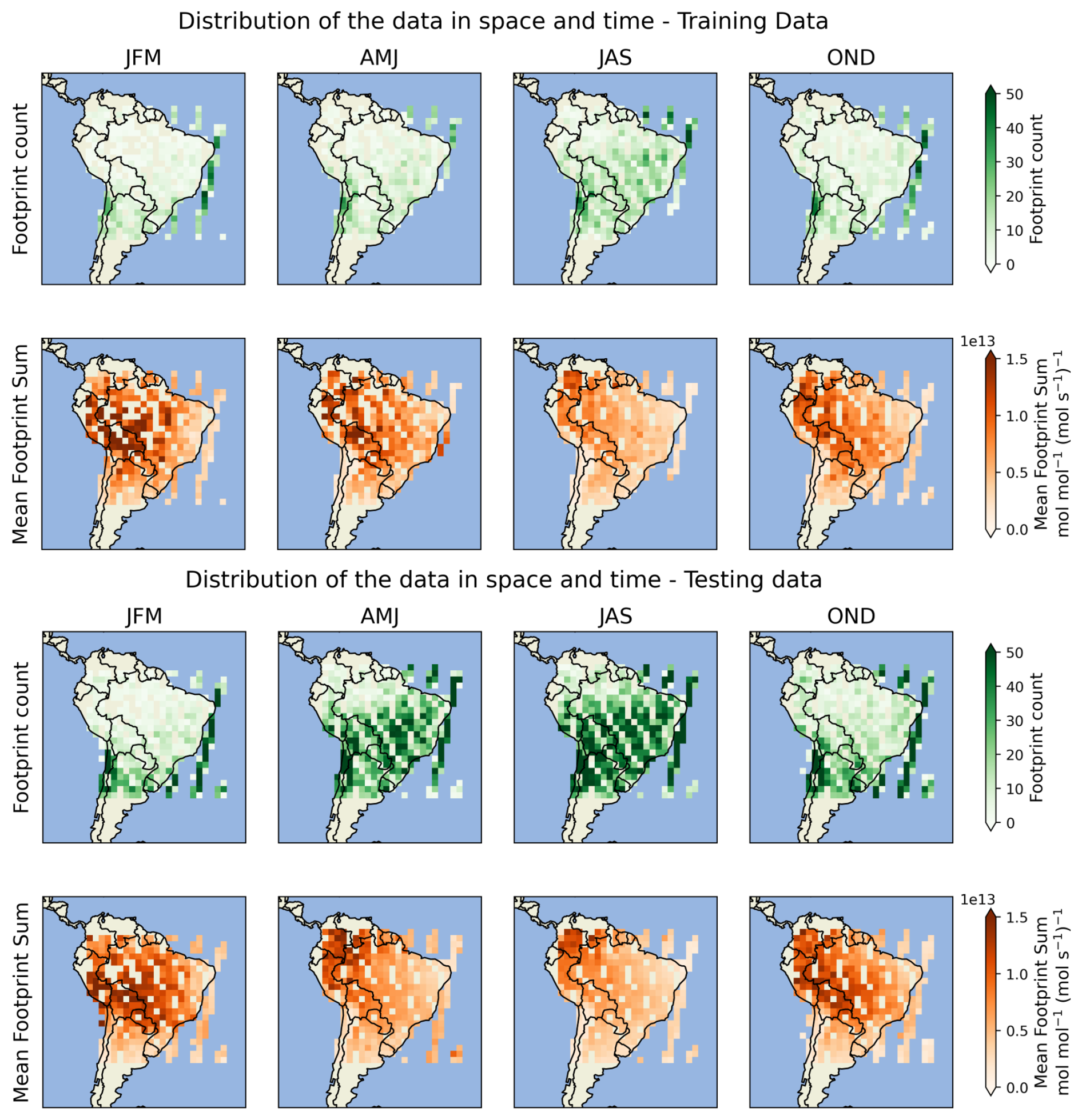
Figure A1 Distribution in space and by season (see key below) of the footprint datasets, split in training (2014–2015, top panel) and validation and testing (2016 and 2018, bottom panel). For each dataset, the count of samples in each 2° bin (top subpanel, green) shows seasonal variations in the data available, with more coverage in July–August–September, as well as spatial biases, with more observations in the southern regions and over the Atlantic. Note that although we train with footprints over the ocean, in the inversion only land observations are used, and we report metrics for those. The bottom subpanels show the mean sum of the footprints in that bin, over the spatial domain (the sensitivity in each grid cell is weighted by the area). Higher mean footprint sums indicate less particle dispersion, often due to slower winds or geographical barriers. For example, mean sums are higher near the Andes, where the high topography prevents the particles from advecting. (Key: JFM = January, February, March, AMJ = April, May, June, JAS = June, July, August, OND = October, November, December).

Appendix B

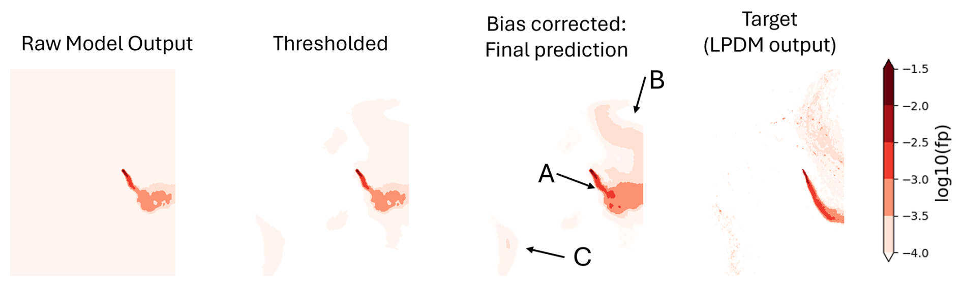
Figure B1 Example of the post-processing method in GATES. The raw prediction from GATES for a particular set of inputs from the test set is shown in the left-most panel. The target footprint predicted by NAME is shown in the right-most panel for comparison. Thresholding is first applied to the emulated footprint, removing all background values under threshold. This threshold is decided from the validation data. A distribution-wise bias correction method, calibrated with the validation data, is then applied, which corrects the magnitude of the footprint values particularly on the tail of the footprint (A) and noisy regions (B and C).

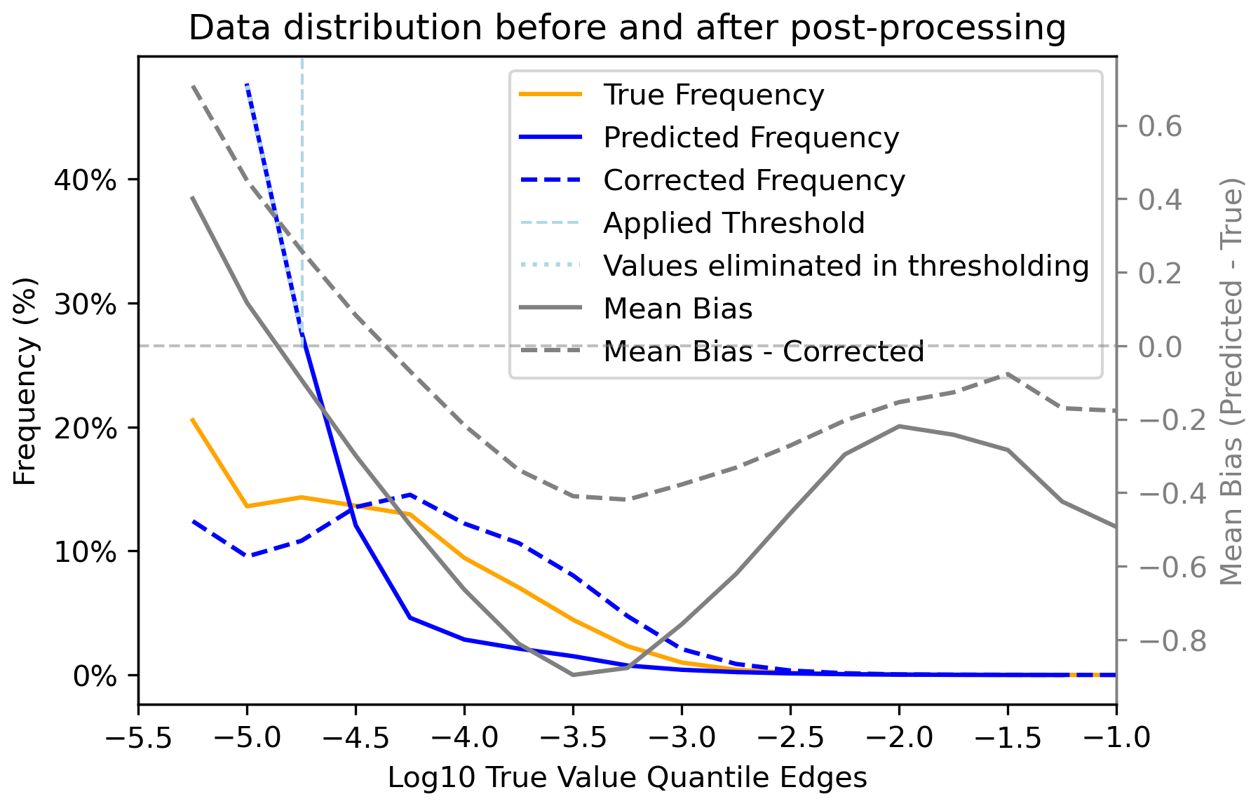
Figure B2 Impact of the bias correction on the data distribution of the test set. In orange we show the logged distribution of the test data (wherever it is non-zero) for April–December 2016 (left axis), split into 20 bins. The distribution of the values predicted directly by GATES is shown with the blue line: there is a very high proportion of small background values. The solid gray line, on the right axes, indicates the mean bias of the raw GATES predictions in each quantile of the true data (in the logged space). GATES tends to under-predict particularly the mid-range values (log(f)≈ −3.5). The post-processing steps are then applied. First we remove background values under a threshold tuned with the validation set (1.757 × 10⁻⁵), indicated by the dashed light blue line. Bias correction is then applied on the remaining values, with the resulting distribution shown as the dashed blue line. The corrected presents an improved fit against the true frequency, and the mean bias of the two distribution with a dashed grey line on the right axes, shows that the mid- and high-range values are better captured.

Appendix C

The emulated footprints are evaluated at three levels: comparing the emulated footprints to the LPDM-generated ones, evaluating the simulated methane column mole fractions, and within an inversion. We use the metrics below to evaluate the model at different levels, where b_i is the true value and $\widehat{b_i}$ is the emulated value.

• 1.

  Pearson's Correlation Coefficient:

  $$r(b,\widehat{b})={\displaystyle \frac{{\sum }_{i=\mathrm{1}}^n\left(b_i-\stackrel{\mathrm{‾}}{b}\right)\left(\widehat{b_i}-\stackrel{\mathrm{‾}}{\widehat{b}}\right)}{\sqrt{{\sum }_{i=\mathrm{1}}^n{\left(b_i-\stackrel{\mathrm{‾}}{b}\right)}^{\mathrm{2}}}\sqrt{{\sum }_{i=\mathrm{1}}^n{\left(\widehat{b_i}-\stackrel{\mathrm{‾}}{\widehat{b}}\right)}^{\mathrm{2}}}}}$$

  The correlation of coefficient is applied to:

  • footprint-to-footprint evaluation. The coefficient of correlation is calculated for each footprint so that $\widehat{b}$ represents the flattened values and comparing them against the flattened corresponding LPDM footprint. The footprint-wise correlations of coefficient can then be shown as averages across different locations or time-periods (Sect. 5.1). It can be applied in the native dataspace, or in the logged dataspace ($r\left(\text{log}\right(b),\text{log}(\widehat{b}\left)\right)$), wherever the footprint is non-zero. This metric ignores the shape of the predicted footprints and evaluates the magnitude only.

  • Mole fraction evaluation: The coefficient of correlation is calculated for the whole dataset of predicted mole fractions. It ignores any time correlation between the data-points.

• 2.

  Intersection Over Union (IoU), also known as Figure of Merit in Space or Jaccard index: quantifies the spatial agreement between the emulated and the true footprints by computing the ratio of the overlapping area to the total area covered by either. It is applied on a binarised version of b above a particular threshold τ=0, so that $B_{i,j}=\mathrm{1}$ if $b_{i,j}>\mathrm{0}$, or $B_{i,j}=\mathrm{0}$ otherwise. IoU score ranges from 0 to 1 (or 0 % to 100 %), where 1 indicates perfect overlap and 0 indicates no overlap at all. The IoU is calculated for each footprint, and averaged across samples in Sect. 5.1.

  $$\text{IoU}(B,\widehat{B})={\displaystyle \frac{\mathrm{|}B\cap \widehat{B}\mathrm{|}}{\mathrm{|}B\cup \widehat{B}\mathrm{|}}}$$
• 3.

  Mean Absolute Error: measures the average absolute difference between the predicted and true values. It is used to evaluate the above-baseline mole fractions (Sect. 5.2), and also the monthly methane emissions for Brazil (Sect. 5.3).

  $$\text{MAE}(b,\widehat{b})={\displaystyle \frac{\mathrm{1}}{n}}{\sum }_{i=\mathrm{1}}^n\left|b_i-\widehat{b_i}\right|$$

• 4.

  Mean Squared Error and Root Mean Squared Error: measure the average of the squared differences between the predicted and true values. The Root MSE (RMSE) is the square root of MSE, the error in the same units as the original data. expressing It is used to evaluate the above-baseline mole fractions (Sect. 5.2).

  $$\begin{array}{ll}{\displaystyle }& {\displaystyle }\text{MSE}(b,\widehat{b})={\displaystyle \frac{\mathrm{1}}{n}}{\sum }_{i=\mathrm{1}}^n{\left(b_i-\widehat{b_i}\right)}^{\mathrm{2}}\\ {\displaystyle }& {\displaystyle }\text{RMSE}=\sqrt{{\displaystyle \frac{\mathrm{1}}{n}}{\sum }_{i=\mathrm{1}}^n{\left(b_i-\widehat{b_i}\right)}^{\mathrm{2}}}\end{array}$$
• 5.

  Mean Bias: measures the average difference between predicted and true values, indicating whether the model systematically overestimates or underestimates with respect to the true value. It is used to evaluate the above-baseline mole fractions (Sect. 5.2), and also the monthly methane emissions for Brazil (Sect. 5.3).

  $$\text{MBE}(b,\widehat{b})={\displaystyle \frac{\mathrm{1}}{n}}{\sum }_{i=\mathrm{1}}^n\left(\widehat{b_i}-b_i\right)$$

Appendix D

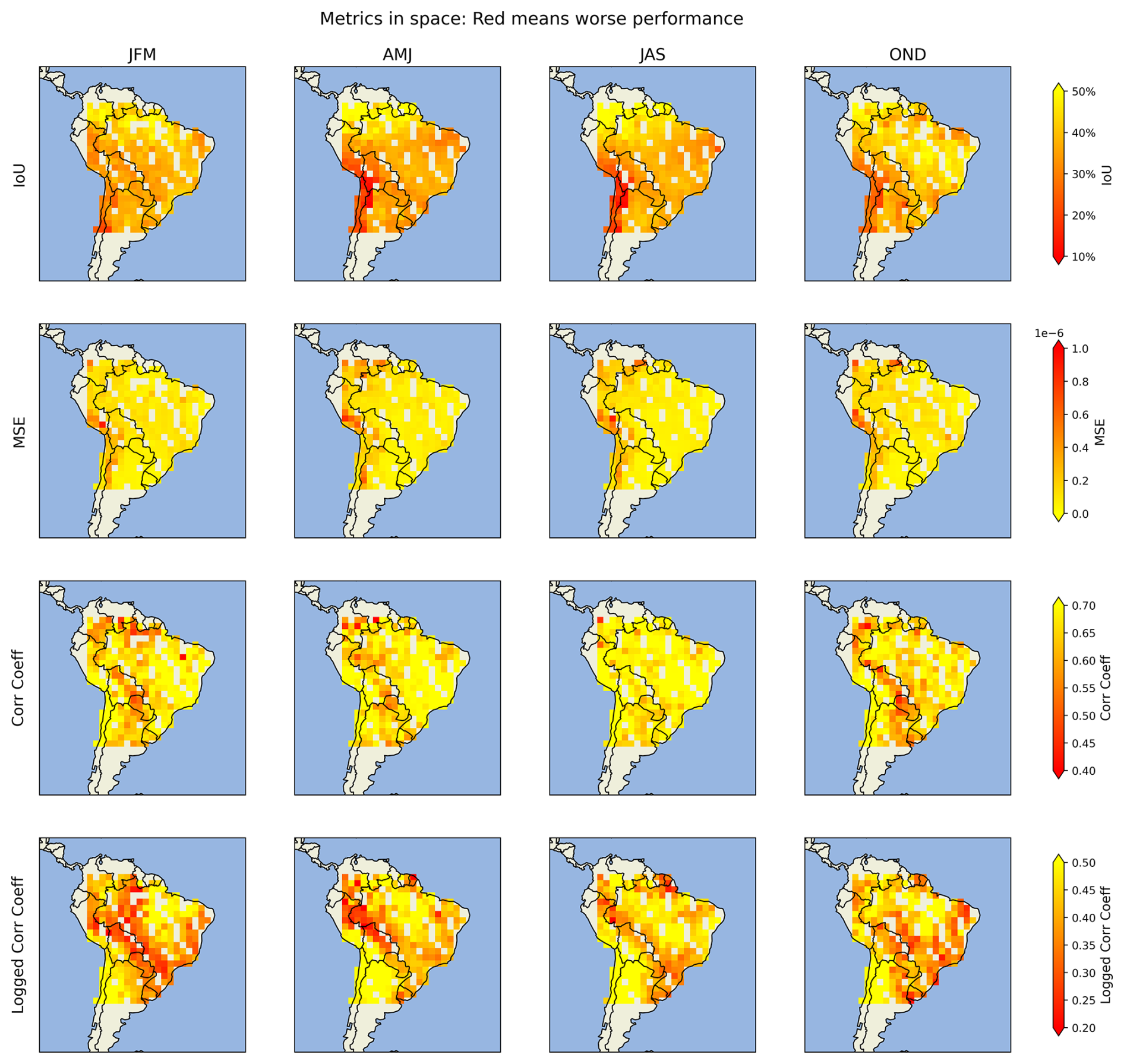
Figure D1 Mean footprint metric scores disaggregated in space and time. Red indicates worse performance for that metric. The footprints are binned by season (see key below) and by the coordinates of the satellite measurements in 2° bins, showing here the mean metrics for each bin in 2016 and 2018. (Key: JFM = January, February, March, AMJ = April, May, June, JAS = June, July, August, OND = October, November, December).

Appendix E

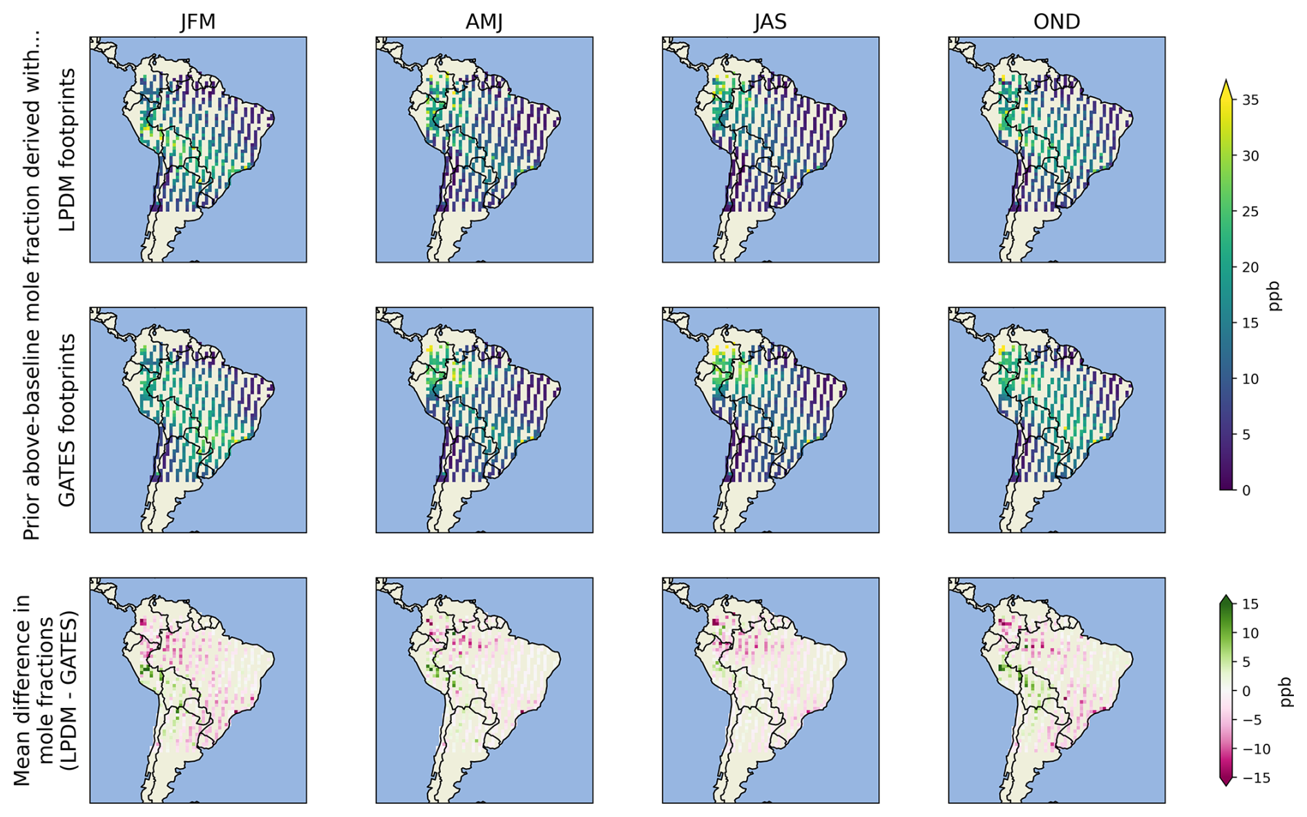
Figure E1 Seasonal mean above-baseline mole fractions, derived with the LPDM footprints (top row), with GATES footprints (middle row) and the difference between the two (bottom row). The mole fractions are derived by convolving a monthly emissions prior with each footprint (see Sect. 5.2 or Tunnicliffe et al. (2020) for a description of the prior). Here, the mole fractions are binned by season (see key below) and in 1° bins, averaged for both 2016 and 2018. The mole fractions calculated with GATES footprints (middle row) show similar spatial patterns to those calculated with LPDM footprints (top row). The two are compared in the bottom row, where positive values (green) indicate mole fractions that were underpredicted by GATES, and negative values (pink) indicate mole fractions that were overpredicted by GATES. (Key: JFM = January, February, March, AMJ = April, May, June, JAS = June, July, August, OND = October, November, December).

Appendix F

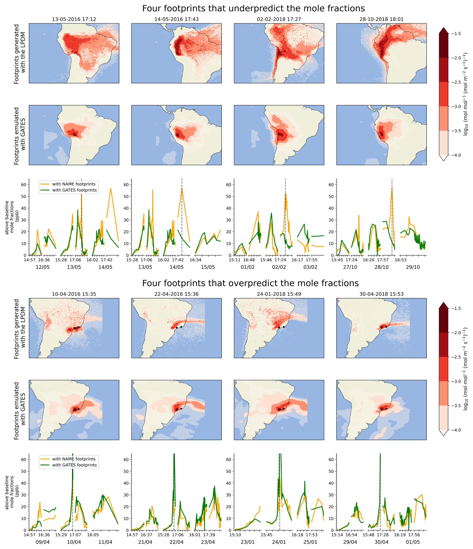
Figure F1 Two sets of footprints that lead to the largest errors in the emulated mole fractions, through underprediction (top panel) or overprediction (bottom panel). In each panel, we show the LPDM footprint (top row), the GATES-emulated footprint (bottom row) and the derived mole-fraction timeseries, for the day of the footprint, the day before and the day after. Top panel: Footprints for measurements near the central Andes area accumulate higher errors than other areas (see Fig. D1), and for these four footprints GATES fails to emulate complex dispersion patterns from difficult meteorology and topography. The LDPM footprints capture dispersion over the Amazon basin, where estimated emissions are large, leading to a big difference between the two estimates. Bottom panel: The smoothing effect is particularly visible here, as sharp, narrow plumes in the LPDM footprints over or near Sao Paulo and Rio de Janeiro (black dots) are emulated to be wider and with softer edges. When convolved with the prior, the large emissions from the cities inflate the small errors in the GATES footprints, leading to overpredictions.

Appendix G

The emissions derived from the inversion can be compared against the actual observations taken by GOSAT. In Fig. G1 (left panel), we show the distribution of prior modelled mole fractions (i.e. footprints × prior fluxes + prior background) for 2018, calculated with the GATES footprints and the LPDM footprints. We also show the distribution of GOSAT XCH₄ observations, and the posterior modelled mole fractions (i.e. footprints × posterior fluxes + posterior background) derived with either set of footprints. Both posteriors fit the observations significantly better than the priors, with most of the improvement attributed to an increase in the background mole fractions. Tunnicliffe et al. (2020) and Thompson et al. (2025) also identify that adjusting the boundary together with the fluxes is key to obtaining well-fitting posteriors. The posteriors derived with either set of footprints are very similar, and show similar error distributions when compared to the observations (Fig. G1, right panel). The prior derived with GATES has a small bias to overpredict mole fractions, which translates into a small bias in the posteriors.

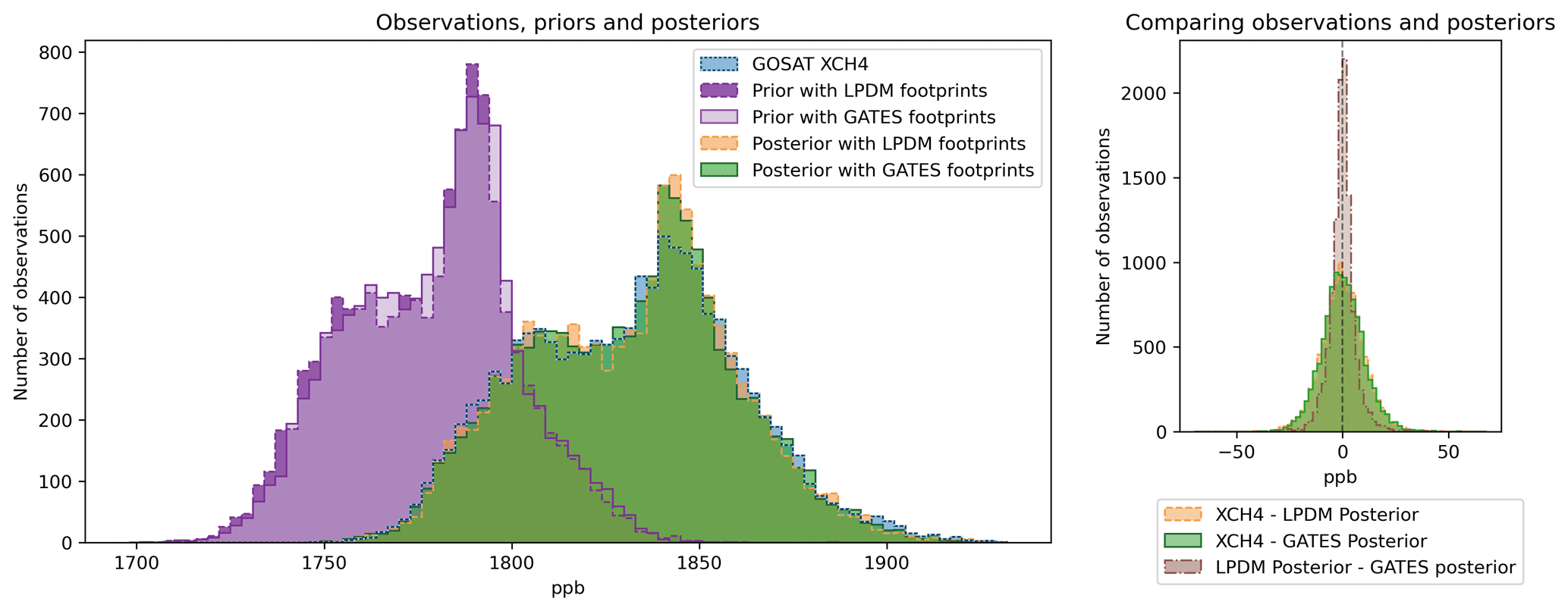
Figure G1 Comparing the distributions of the GOSAT observations, prior and posterior mole fractions in 2018. Left panel: Distributions for a priori modelled methane mole fractions (dark and light purple), GOSAT XCH₄ observations (blue) and the posterior mole fractions (orange and green). We show the prior and posterior pair generated with the LPDM footprints (purple and orange, respectively, dashed edges) and the posterior and prior pair generated with the GATES footprints (purple and green, respectively, solid edges). Both posteriors fit the observations well. Right panel: Distribution of errors between the XCH₄ observations and the mole fractions calculated from both sets of posteriors (in orange and green), and differences between the mole fractions derived with both posteriors (brown). Both posteriors show similar error patterns between the estimated emissions and the actual XCH₄ observations. The errors between the two posteriors (brown) are normally distributed, with a small positive mean bias (2.69 ppb) which indicates a small overpredicting tendency in GATES.