Implementation of a sigma coordinate system in PALM-Sigma v1.0 (based on PALM v21.10) for LES study of the marine atmospheric boundary layer

In large-eddy simulation studies of the marine atmospheric boundary layer, wind-wave interactions are often oversimplified using wall-stress models parameterized by roughness length, overlooking the complex coupling dynamics, especially under wind-wave non-equilibrium states. Here, we develop a wave-phase-resolved solver that employs a surface-following sigma coordinate system to explicitly resolve evolving wave geometry. Simulations under low-wind conditions with different wave regimes reproduce characteristic features of wave-driven winds reported in previous studies. Notably, the results show that wave-induced form stress significantly modulates vertical momentum flux, with effects extending well beyond the wave boundary layer. Built on PALM’s framework, the solver can be seamlessly integrated with the multi-scale nesting module and coupled with wave models, enabling high-fidelity simulations to improve understanding and parameterization of wind-wave coupling under realistic conditions.

1 Introduction

The ocean surface is characterized by ubiquitous waves with a wide range of amplitudes and propagating speeds. These waves induce perturbations to the velocity and pressure fields of the overlying atmospheric boundary layer flow and modify the exchange of mass, momentum, and heat between the atmosphere and the ocean (Sullivan and McWilliams, 2010). Although the wave-induced disturbances are known to decay with height by an exponential rate (Donelan et al., 2006), numerous studies demonstrate that the surface waves have profound influences on the wind field above (Peña and Gryning, 2008; Grare et al., 2018; Chen et al., 2019), especially in conditions with the presence of swells under relatively low wind speed (Grachev and Fairall, 2001; Hanley and Belcher, 2008). A deep understanding of this atmosphere-wave interaction process is thus beneficial for the study of marine meteorology and relevant applications from weather forecasting to offshore wind energy. However, this problem remains a challenging topic in both theoretical and experimental researches due to the complexity of physics and demanding requirements for the measurement devices. More work is necessary to obtain a comprehensive knowledge of the wave-induced effects on the marine atmospheric boundary layer (MABL). Over the past two decades, the numerical modeling tools, especially the large-eddy simulation technique, have experienced rapid development and been widely used in the area of micro-scale meteorology. Already in 2018, high-performance computing (HPC) equipment enabled numerical simulations with a magnitude of up to 10¹⁰ grid points (Kröniger et al., 2018). The ability to resolve 3D flow field with high temporal-spatial resolution makes large-eddy simulation a promising tool to study the wave-coherent flow in the vicinity of the wave surface and its effects on the boundary layer structure.

In numerical modeling of MABL flows, wave effects are typically incorporated using two main approaches (Deskos et al., 2021). The first is a wave-phase-averaged method, where wave-induced stress near the surface is parameterized using empirical formulations based on wind-wave conditions. The second is a wave-phase-resolved approach, in which the geometry of the wavy sea surface is explicitly represented at the bottom boundary, allowing the flow disturbances generated by surface motions to be directly resolved. Considering its simplicity and low cost, the first approach is used in most of the current simulation tools. Nevertheless, the reliability of parameterizations shows dependence on site and wave types (Drennan et al., 2005; Jiménez and Dudhia, 2018), and there is no universal method with satisfying performance in any wind-sea environments. By contrast, the second approach has a more accurate representation of the physics of the airflow-water interaction process by involving the information of wave motions as the boundary condition. This enables the wave-phase-resolved simulator to reproduce the coupling dynamics in various wind-sea regimes and stability conditions, e.g., wind-wave misalignment and upwards wave-induced momentum flux in swell conditions (Smedman et al., 1999, 2009). Therefore, many research groups have developed numerical simulation tools with wave-phase-resolving capability in order to study the dynamics of turbulent flow affected by different types of waves.

The direct numerical simulation (DNS) studies by Sullivan et al. (2000), Sullivan and McWilliams (2002), Shen et al. (2003), Kihara et al. (2007), and Yang and Shen (2009, 2010) provided detailed flow field information in the vicinity of water surface and valuable interpretations of the process and mechanism of wind-wave interaction. Such direct numerical simulations must be confined to a low Reynolds number due to the high computational cost for resolving the wall boundary layer flow. Compared with DNS, LES has no such limitation if a wall-layer model is applied to estimate the surface stress by the Monin-Obukhov similarity theory (MOST). This makes the LES model a powerful tool to study the wave-induced effects on MABL in more realistic scenarios. Sullivan et al. (2008, 2014) considered monochromatic and broadband-spectral waves and a wide range of geostrophic wind speeds in his LES study. His simulations illustrated that both the mean wind profile and the turbulence in MABL can be strongly affected by waves. The balance between the turbulent friction, wave-induced form stress, and subgrid-scale (SGS) stress depends on the wave age (the ratio between wave phase speed and friction velocity) and the distance above the water surface. Hao and Shen (2019) performed a two-way wind-wave coupling simulation using LES and potential flow solver to solve wind turbulence and wave field, respectively. They found the phenomenon of the frequency shift in the wind-wave spectrum and the enhanced turbulent shear stress from sweep events as a result of waves. In addition, as the fast growing offshore wind energy industry draws increasing attention over the world, the wave-phase-resolved LES technique has also been used in the studies of the wake dynamics of wind turbines in the MABL. For example, Yang et al. (2014) investigated the wind farm performance under fetch-limited and fully developed wave conditions and indicated that the latter situation with lower surface drag leads to an increase of 8 % for the power extraction rate. The recent series of LES studies by Yang et al. (2022b, a) were focused on swell-dominant regimes. They found that the power output of a wind turbine can increase by nearly one time under the influence of fast propagating wind-following swells, and the recovery of wake flow is also affected through enhanced or mitigated turbulence due to the presence of waves.

The above numerical work contributes greatly to our understanding of how the characteristics of wind field change while interacting with the underlying wave surface, but there are still knowledge gaps in wind-wave coupling problem with more complex environmental conditions, such as non-neutral atmospheric stability and the wake flow of large-scale wind farms. This becomes the main motivation for our present work to extend the PALM code with the ability to solve the turbulent flow over a wavy surface. PALM is a widely used and well maintained code developed by the group from Leibniz Universitat Hannover (LUH) (Maronga et al., 2020) since 20 years ago. It is designed for highly parallelized simulations of atmospheric and oceanic boundary layer flows and is embedded with many practical sub-models, such as meso-to-micro scale nesting interface, Lagrangian particle model, and wind turbine model, which makes PALM a powerful tool in diverse research fields. The current work further develops PALM to a wave-phase-resolved simulator (PALM-Sigma) through the implementation of a sigma coordinate system and pave the way for its application in future studies related to MABL flow and offshore wind energy engineering. We first present the governing equations and their numerical implementation in Sects. 2 and 3, followed by an overview of the code framework in Sect. 4. Section 5 describes the simulation setup and case configurations. The results are discussed in detail in Sect. 6, and finally, Sect. 7 provides a summary and outlines directions for future work.

2 Governing equations

2.1 Governing equations in Cartesian coordinates

We briefly summarize the governing equations of the original PALM model system in this subsection as the foundation for our subsequent implementation of sigma coordinates. PALM is a large-eddy simulation model that solves the incompressible Navier-Stokes equations. Specifically, the equations consist of the continuity equation, the momentum equation, and the scalar transport equation:

$$\begin{array}{}\text{(1)}& {\displaystyle \frac{\partial u_j}{\partial x_j}}=\mathrm{0},\text{(2)}& {\displaystyle }\begin{array}{rl}{\displaystyle \frac{\partial u_i}{\partial t}}& =-{\displaystyle \frac{\partial u_i{u}_j}{\partial x_j}}-{\mathit{\epsilon }}_{ijk}{f}_j{u}_k+{\mathit{\epsilon }}_{i\mathrm{3}j}{f}_{\mathrm{3}}{u}_{\mathrm{g},j}-{\displaystyle \frac{\mathrm{1}}{{\mathit{\rho }}_{\mathrm{0}}}}{\displaystyle \frac{\partial {\mathit{\pi }}^{*}}{\partial x_i}}\\ & +g{\displaystyle \frac{{\mathit{\theta }}_{\mathrm{v}}-\langle {\mathit{\theta }}_{\mathrm{v}}\rangle }{\langle {\mathit{\theta }}_{\mathrm{v}}\rangle }}{\mathit{\delta }}_{i\mathrm{3}}-{\displaystyle \frac{\partial }{\partial x_j}}\left(\stackrel{\mathrm{‾}}{u_i^{\prime \prime }{u}_j^{\prime \prime }}-{\displaystyle \frac{\mathrm{2}}{\mathrm{3}}}e{\mathit{\delta }}_{ij}\right),\end{array}\text{(3)}& {\displaystyle \frac{\partial \mathit{\varphi }}{\partial t}}=-{\displaystyle \frac{\partial u_j\mathit{\varphi }}{\partial x_j}}-{\displaystyle \frac{\partial \stackrel{\mathrm{‾}}{u_j^{\prime \prime }{\mathit{\varphi }}^{\prime \prime }}}{\partial x_j}}+{\mathrm{\Psi }}_{\mathit{\varphi }}.\end{array}$$

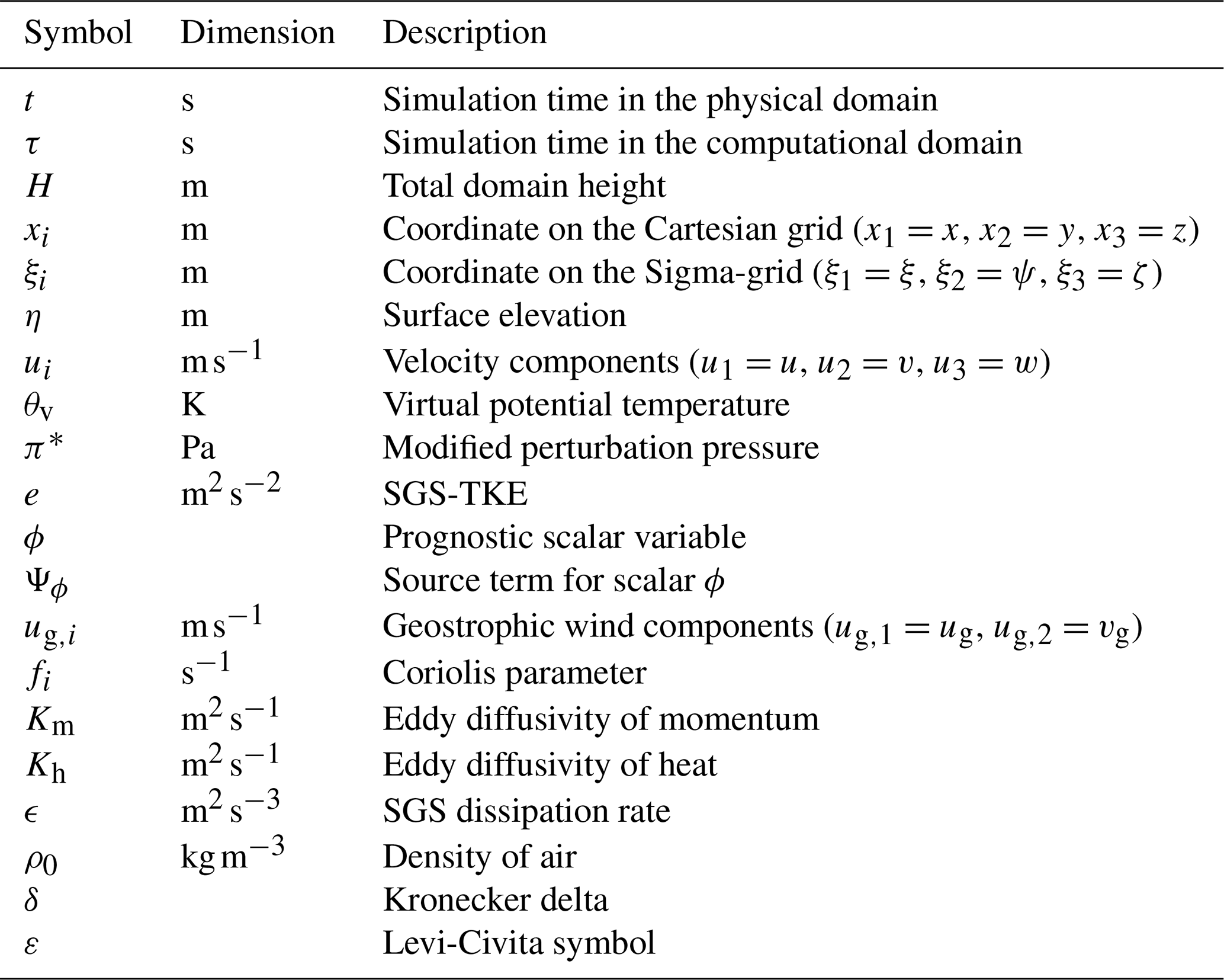
Symbols ϵ and δ represent the Levi-Civita tensor and Kronecker delta, respectively. t is time, and x_i, x_j, x_k denote spatial coordinates, with indices i, j, $k\in \mathrm{1},\mathrm{2},\mathrm{3}$. u_i, u_j, and u_k denote the components of velocity. π^* represents the modified perturbation pressure, and θ_v stands for the virtual potential temperature, and 〈θ_v〉 is its horizontal average. ϕ represents a generic transported scalar, and Ψ_ϕ is its source term. These prognostic variables are resolved-scale quantities, with the filtering notation omitted for clarity. g is the gravitational acceleration. f denotes the Coriolis parameter with the latitude ϕ set at 54°. ρ₀ is the density of dry air. The overbar denotes Reynolds averaging, and the double prime indicates subgrid-scale (SGS) components. e represents the subgrid-scale turbulent kinetic energy (SGS-TKE).

2.2 Coordinate transformation

The wavy ocean surface introduces a dynamic and curvy lower boundary to the MABL, which poses significant challenges for numerical modeling in a traditional Cartesian coordinate system. To explicitly resolve the wave geometry and its interaction with the flow, the PALM model has been extended with a sigma coordinate system. This transformation normalizes the vertical coordinate by the instantaneous local domain height, defined as the distance between the evolving wave surface and the fixed upper boundary, while retaining Cartesian coordinates in the horizontal directions. The coordinate transformation is given by:

$$\begin{array}{}\text{(4)}& \mathit{\tau }=t,\mathit{\xi }=x,\mathit{\psi }=y,\mathit{\zeta }={\displaystyle \frac{z-\mathit{\eta }}{H-\mathit{\eta }}},\end{array}$$

where η denotes wave surface elevation and H is the total vertical extent of the domain. τ, ξ, ψ, ζ (or equivalently ξ₁=ξ, ξ₂=ψ, ξ₃=ζ) are the time and space coordinates in the computational domain. The derivative terms in Cartesian coordinates can then be reformulated by the chain rule as

$$\begin{array}{}\text{(5)}& {\displaystyle }\begin{array}{rl}& {\displaystyle \frac{\partial }{\partial t}}={\displaystyle \frac{\partial }{\partial \mathit{\tau }}}+{\mathit{\zeta }}_t{\displaystyle \frac{\partial }{\partial \mathit{\zeta }}},{\displaystyle \frac{\partial }{\partial x}}={\displaystyle \frac{\partial }{\partial \mathit{\xi }}}+{\mathit{\zeta }}_x{\displaystyle \frac{\partial }{\partial \mathit{\zeta }}},\\ & {\displaystyle \frac{\partial }{\partial y}}={\displaystyle \frac{\partial }{\partial \mathit{\psi }}}+{\mathit{\zeta }}_y{\displaystyle \frac{\partial }{\partial \mathit{\zeta }}},{\displaystyle \frac{\partial }{\partial z}}={\mathit{\zeta }}_z{\displaystyle \frac{\partial }{\partial \mathit{\zeta }}},\end{array}\text{(6)}& {\displaystyle }\begin{array}{rl}& {\displaystyle \frac{{\partial }^{\mathrm{2}}}{\partial x^{\mathrm{2}}}}={\displaystyle \frac{{\partial }^{\mathrm{2}}}{\partial {\mathit{\xi }}^{\mathrm{2}}}}+\mathrm{2}{\mathit{\zeta }}_x{\displaystyle \frac{{\partial }^{\mathrm{2}}}{\partial \mathit{\xi }\partial \mathit{\zeta }}}+{\mathit{\zeta }}_x^{\mathrm{2}}{\displaystyle \frac{{\partial }^{\mathrm{2}}}{\partial {\mathit{\zeta }}^{\mathrm{2}}}}+{\mathit{\zeta }}_{xx}{\displaystyle \frac{\partial }{\partial \mathit{\zeta }}},\\ & {\displaystyle \frac{{\partial }^{\mathrm{2}}}{\partial y^{\mathrm{2}}}}={\displaystyle \frac{{\partial }^{\mathrm{2}}}{\partial {\mathit{\psi }}^{\mathrm{2}}}}+\mathrm{2}{\mathit{\zeta }}_y{\displaystyle \frac{{\partial }^{\mathrm{2}}}{\partial \mathit{\psi }\partial \mathit{\zeta }}}+{\mathit{\zeta }}_y^{\mathrm{2}}{\displaystyle \frac{{\partial }^{\mathrm{2}}}{\partial {\mathit{\zeta }}^{\mathrm{2}}}}+{\mathit{\zeta }}_{yy}{\displaystyle \frac{\partial }{\partial \mathit{\zeta }}},\\ & {\displaystyle \frac{{\partial }^{\mathrm{2}}}{\partial z^{\mathrm{2}}}}={\mathit{\zeta }}_z^{\mathrm{2}}{\displaystyle \frac{{\partial }^{\mathrm{2}}}{\partial {\mathit{\zeta }}^{\mathrm{2}}}}.\end{array}\end{array}$$

The derivatives of ζ with respect to the original coordinates, commonly referred to as metric terms (Pletcher et al., 2012), establish the mathematical relationship between the physical and computational domains. These metric terms are expressed as

$$\begin{array}{}\text{(7)}& {\displaystyle }\begin{array}{rl}{\mathit{\zeta }}_t& ={\displaystyle \frac{\mathit{\zeta }-\mathrm{1}}{H-\mathit{\eta }}}{\mathit{\eta }}_t,{\mathit{\zeta }}_x={\displaystyle \frac{\mathit{\zeta }-\mathrm{1}}{H-\mathit{\eta }}}{\mathit{\eta }}_x,{\mathit{\zeta }}_y={\displaystyle \frac{\mathit{\zeta }-\mathrm{1}}{H-\mathit{\eta }}}{\mathit{\eta }}_y,\\ {\mathit{\zeta }}_z& ={\displaystyle \frac{\mathrm{1}}{H-\mathit{\eta }}},\end{array}\text{(8)}& {\displaystyle }\begin{array}{rl}& {\mathit{\zeta }}_{xx}={\displaystyle \frac{\mathrm{2}(\mathit{\zeta }-\mathrm{1})}{(H-\mathit{\eta }{)}^{\mathrm{2}}}}{\mathit{\eta }}_x^{\mathrm{2}}+{\displaystyle \frac{\mathit{\zeta }-\mathrm{1}}{H-\mathit{\eta }}}{\mathit{\eta }}_{xx},\\ & {\mathit{\zeta }}_{yy}={\displaystyle \frac{\mathrm{2}(\mathit{\zeta }-\mathrm{1})}{(H-\mathit{\eta }{)}^{\mathrm{2}}}}{\mathit{\eta }}_y^{\mathrm{2}}+{\displaystyle \frac{\mathit{\zeta }-\mathrm{1}}{H-\mathit{\eta }}}{\mathit{\eta }}_{yy}.\end{array}\end{array}$$

2.3 Governing equations in Sigma coordinates

By applying the above mesh transformation to the original governing equations in PALM, we obtain the Navier-Stokes equations and scalar transport equation in the sigma coordinate system:

$$\begin{array}{}\text{(9)}& {\displaystyle \frac{\partial u}{\partial \mathit{\xi }}}+{\mathit{\zeta }}_x{\displaystyle \frac{\partial u}{\partial \mathit{\zeta }}}+{\displaystyle \frac{\partial v}{\partial \mathit{\psi }}}+{\mathit{\zeta }}_y{\displaystyle \frac{\partial v}{\partial \mathit{\zeta }}}+{\mathit{\zeta }}_z{\displaystyle \frac{\partial w}{\partial \mathit{\zeta }}}=\mathrm{0},\text{(10)}& {\displaystyle }\begin{array}{rl}{\displaystyle \frac{\partial u}{\partial \mathit{\tau }}}& +{\mathit{\zeta }}_t{\displaystyle \frac{\partial u}{\partial \mathit{\zeta }}}=-\left({\displaystyle \frac{\partial uu}{\partial \mathit{\xi }}}+{\mathit{\zeta }}_x{\displaystyle \frac{\partial uu}{\partial \mathit{\zeta }}}\right)-\left({\displaystyle \frac{\partial uv}{\partial \mathit{\psi }}}+{\mathit{\zeta }}_y{\displaystyle \frac{\partial uv}{\partial \mathit{\zeta }}}\right)\\ & -{\mathit{\zeta }}_z{\displaystyle \frac{\partial uw}{\partial \mathit{\zeta }}}-f_{\mathrm{2}}w+f_{\mathrm{3}}(v-v_{\mathrm{g}})-{\displaystyle \frac{\mathrm{1}}{{\mathit{\rho }}_{\mathrm{0}}}}\left({\displaystyle \frac{\partial {\mathit{\pi }}^{*}}{\partial \mathit{\xi }}}+{\mathit{\zeta }}_x{\displaystyle \frac{\partial {\mathit{\pi }}^{*}}{\partial \mathit{\zeta }}}\right)\\ & -\left({\displaystyle \frac{\partial }{\partial \mathit{\xi }}}+{\mathit{\zeta }}_x{\displaystyle \frac{\partial }{\partial \mathit{\zeta }}}\right)\left(\stackrel{\mathrm{‾}}{u^{\prime \prime }{u}^{\prime \prime }}-{\displaystyle \frac{\mathrm{2}}{\mathrm{3}}}e\right)\\ & -\left({\displaystyle \frac{\partial }{\partial \mathit{\psi }}}+{\mathit{\zeta }}_y{\displaystyle \frac{\partial }{\partial \mathit{\zeta }}}\right)\left(\stackrel{\mathrm{‾}}{u^{\prime \prime }{v}^{\prime \prime }}\right)-{\mathit{\zeta }}_z{\displaystyle \frac{\partial }{\partial \mathit{\zeta }}}\left(\stackrel{\mathrm{‾}}{u^{\prime \prime }{w}^{\prime \prime }}\right),\end{array}\text{(11)}& {\displaystyle }\begin{array}{rl}{\displaystyle \frac{\partial v}{\partial \mathit{\tau }}}& +{\mathit{\zeta }}_t{\displaystyle \frac{\partial v}{\partial \mathit{\zeta }}}=-\left({\displaystyle \frac{\partial vu}{\partial \mathit{\xi }}}+{\mathit{\zeta }}_x{\displaystyle \frac{\partial vu}{\partial \mathit{\zeta }}}\right)-\left({\displaystyle \frac{\partial vv}{\partial \mathit{\psi }}}+{\mathit{\zeta }}_y{\displaystyle \frac{\partial vv}{\partial \mathit{\zeta }}}\right)\\ & -{\mathit{\zeta }}_z{\displaystyle \frac{\partial vw}{\partial \mathit{\zeta }}}-f_{\mathrm{3}}(u-u_{\mathrm{g}})-{\displaystyle \frac{\mathrm{1}}{{\mathit{\rho }}_{\mathrm{0}}}}\left({\displaystyle \frac{\partial {\mathit{\pi }}^{*}}{\partial \mathit{\psi }}}+{\mathit{\zeta }}_y{\displaystyle \frac{\partial {\mathit{\pi }}^{*}}{\partial \mathit{\zeta }}}\right)\\ & -\left({\displaystyle \frac{\partial }{\partial \mathit{\xi }}}+{\mathit{\zeta }}_x{\displaystyle \frac{\partial }{\partial \mathit{\zeta }}}\right)\left(\stackrel{\mathrm{‾}}{v^{\prime \prime }{u}^{\prime \prime }}\right)\\ & -\left({\displaystyle \frac{\partial }{\partial \mathit{\psi }}}+{\mathit{\zeta }}_y{\displaystyle \frac{\partial }{\partial \mathit{\zeta }}}\right)\left(\stackrel{\mathrm{‾}}{v^{\prime \prime }{v}^{\prime \prime }}-{\displaystyle \frac{\mathrm{2}}{\mathrm{3}}}e\right)-{\mathit{\zeta }}_z{\displaystyle \frac{\partial }{\partial \mathit{\zeta }}}\left(\stackrel{\mathrm{‾}}{v^{\prime \prime }{w}^{\prime \prime }}\right),\end{array}\text{(12)}& {\displaystyle }\begin{array}{rl}{\displaystyle \frac{\partial w}{\partial \mathit{\tau }}}& +{\mathit{\zeta }}_t{\displaystyle \frac{\partial w}{\partial \mathit{\zeta }}}=-\left({\displaystyle \frac{\partial wu}{\partial \mathit{\xi }}}+{\mathit{\zeta }}_x{\displaystyle \frac{\partial wu}{\partial \mathit{\zeta }}}\right)-\left({\displaystyle \frac{\partial wv}{\partial \mathit{\psi }}}+{\mathit{\zeta }}_y{\displaystyle \frac{\partial wv}{\partial \mathit{\zeta }}}\right)\\ & -{\mathit{\zeta }}_z{\displaystyle \frac{\partial ww}{\partial \mathit{\zeta }}}+f_{\mathrm{2}}u+g{\displaystyle \frac{{\mathit{\theta }}_{\mathrm{v}}-{\mathit{\theta }}_{\mathrm{v},\text{ref}}}{{\mathit{\theta }}_{\mathrm{v},\text{ref}}}}-{\displaystyle \frac{\mathrm{1}}{{\mathit{\rho }}_{\mathrm{0}}}}\left({\mathit{\zeta }}_z{\displaystyle \frac{\partial {\mathit{\pi }}^{*}}{\partial \mathit{\zeta }}}\right)\\ & -\left({\displaystyle \frac{\partial }{\partial \mathit{\xi }}}+{\mathit{\zeta }}_x{\displaystyle \frac{\partial }{\partial \mathit{\zeta }}}\right)\left(\stackrel{\mathrm{‾}}{w^{\prime \prime }{u}^{\prime \prime }}\right)-\left({\displaystyle \frac{\partial }{\partial \mathit{\psi }}}+{\mathit{\zeta }}_y{\displaystyle \frac{\partial }{\partial \mathit{\zeta }}}\right)\left(\stackrel{\mathrm{‾}}{w^{\prime \prime }{v}^{\prime \prime }}\right)\\ & -{\mathit{\zeta }}_z{\displaystyle \frac{\partial }{\partial \mathit{\zeta }}}\left(\stackrel{\mathrm{‾}}{w^{\prime \prime }{w}^{\prime \prime }}-{\displaystyle \frac{\mathrm{2}}{\mathrm{3}}}e\right),\end{array}\text{(13)}& {\displaystyle }\begin{array}{rl}{\displaystyle \frac{\partial \mathit{\varphi }}{\partial \mathit{\tau }}}& +{\mathit{\zeta }}_t{\displaystyle \frac{\partial \mathit{\varphi }}{\partial \mathit{\zeta }}}=-\left({\displaystyle \frac{\partial u\mathit{\varphi }}{\partial \mathit{\xi }}}+{\mathit{\zeta }}_x{\displaystyle \frac{\partial u\mathit{\varphi }}{\partial \mathit{\zeta }}}\right)-\left({\displaystyle \frac{\partial v\mathit{\varphi }}{\partial \mathit{\psi }}}+{\mathit{\zeta }}_y{\displaystyle \frac{\partial v\mathit{\varphi }}{\partial \mathit{\zeta }}}\right)\\ & -{\mathit{\zeta }}_z{\displaystyle \frac{\partial w\mathit{\varphi }}{\partial \mathit{\zeta }}}-\left({\displaystyle \frac{\partial }{\partial \mathit{\xi }}}+{\mathit{\zeta }}_x{\displaystyle \frac{\partial }{\partial \mathit{\zeta }}}\right)\left(\stackrel{\mathrm{‾}}{u^{\prime \prime }{\mathit{\varphi }}^{\prime \prime }}\right)\\ & -\left({\displaystyle \frac{\partial }{\partial \mathit{\psi }}}+{\mathit{\zeta }}_y{\displaystyle \frac{\partial }{\partial \mathit{\zeta }}}\right)\left(\stackrel{\mathrm{‾}}{v^{\prime \prime }{\mathit{\varphi }}^{\prime \prime }}\right)-{\mathit{\zeta }}_z{\displaystyle \frac{\partial }{\partial \mathit{\zeta }}}\left(\stackrel{\mathrm{‾}}{w^{\prime \prime }{\mathit{\varphi }}^{\prime \prime }}\right)+{\mathrm{\Psi }}_{\mathit{\varphi }}.\end{array}\end{array}$$

As in the original PALM code, the SGS fluxes are modeled using an eddy diffusivity approach, where the flux is proportional to the gradient of the corresponding variable. However, due to the mesh transformation, additional gradient terms involving the metric terms arise. The resulting expressions for the momentum and scalar fluxes are given by

$$\begin{array}{}\text{(14)}& {\displaystyle }\stackrel{\mathrm{‾}}{u_i^{\prime \prime }{u}_j^{\prime \prime }}-{\displaystyle \frac{\mathrm{2}}{\mathrm{3}}}e{\mathit{\delta }}_{ij}=-K_{\mathrm{m}}\left({\displaystyle \frac{\partial {\mathit{\xi }}_k}{\partial x_j}}{\displaystyle \frac{\partial u_i}{\partial {\mathit{\xi }}_k}}+{\displaystyle \frac{\partial {\mathit{\xi }}_k}{\partial x_i}}{\displaystyle \frac{\partial u_j}{\partial {\mathit{\xi }}_k}}\right),\text{(15)}& {\displaystyle }\stackrel{\mathrm{‾}}{u_i^{\prime \prime }{\mathit{\varphi }}^{\prime \prime }}=-K_{\mathrm{h}}\left({\displaystyle \frac{\partial {\mathit{\xi }}_k}{\partial x_i}}{\displaystyle \frac{\partial \mathit{\varphi }}{\partial {\mathit{\xi }}_k}}\right).\end{array}$$

Multiple options of SGS parameterizations can be used to estimate the eddy diffusivities (K_m and K_h), including the modified Deardorff models (Deardorff, 1980; Moeng and Wyngaard, 1988; Saiki et al., 2000) and the dynamic SGS model (Germano et al., 1991). These models compute eddy diffusivities based on the local grid resolution and the strength of subgrid-scale turbulent kinetic energy. The SGS-TKE is obtained by solving the following prognostic equation:

$$\begin{array}{}\text{(16)}& \begin{array}{rl}{\displaystyle \frac{\partial e}{\partial \mathit{\tau }}}& +{\mathit{\zeta }}_t{\displaystyle \frac{\partial e}{\partial \mathit{\zeta }}}=-u\left({\displaystyle \frac{\partial e}{\partial \mathit{\xi }}}+{\mathit{\zeta }}_x{\displaystyle \frac{\partial e}{\partial \mathit{\zeta }}}\right)-v\left({\displaystyle \frac{\partial e}{\partial \mathit{\psi }}}+{\mathit{\zeta }}_y{\displaystyle \frac{\partial e}{\partial \mathit{\zeta }}}\right)\\ & -w\left({\mathit{\zeta }}_z{\displaystyle \frac{\partial e}{\partial \mathit{\zeta }}}\right)-\stackrel{\mathrm{‾}}{u_j^{\prime \prime }{u}^{\prime \prime }}\left({\displaystyle \frac{\partial u_j}{\partial \mathit{\xi }}}+{\mathit{\zeta }}_x{\displaystyle \frac{\partial u_j}{\partial \mathit{\zeta }}}\right)\\ & -\stackrel{\mathrm{‾}}{u_j^{\prime \prime }{v}^{\prime \prime }}\left({\displaystyle \frac{\partial u_j}{\partial \mathit{\psi }}}+{\mathit{\zeta }}_y{\displaystyle \frac{\partial u_j}{\partial \mathit{\zeta }}}\right)-\stackrel{\mathrm{‾}}{u_j^{\prime \prime }{w}^{\prime \prime }}\left({\mathit{\zeta }}_z{\displaystyle \frac{\partial u_j}{\partial \mathit{\zeta }}}\right)\\ & -\left({\displaystyle \frac{\partial }{\partial \mathit{\xi }}}+{\mathit{\zeta }}_x{\displaystyle \frac{\partial }{\partial \mathit{\zeta }}}\right)\left[-\mathrm{2}{K}_{\mathrm{m}}\left({\displaystyle \frac{\partial e}{\partial \mathit{\xi }}}+{\mathit{\zeta }}_x{\displaystyle \frac{\partial e}{\partial \mathit{\zeta }}}\right)\right]\\ & -\left({\displaystyle \frac{\partial }{\partial \mathit{\psi }}}+{\mathit{\zeta }}_y{\displaystyle \frac{\partial }{\partial \mathit{\zeta }}}\right)\left[-\mathrm{2}{K}_{\mathrm{m}}\left({\displaystyle \frac{\partial e}{\partial \mathit{\psi }}}+{\mathit{\zeta }}_y{\displaystyle \frac{\partial e}{\partial \mathit{\zeta }}}\right)\right]\\ & -{\mathit{\zeta }}_z{\displaystyle \frac{\partial }{\partial \mathit{\zeta }}}\left[-\mathrm{2}{K}_{\mathrm{m}}\left({\mathit{\zeta }}_z{\displaystyle \frac{\partial e}{\partial \mathit{\zeta }}}\right)\right]+{\displaystyle \frac{g}{{\mathit{\theta }}_{\mathrm{v},\mathrm{0}}}}\stackrel{\mathrm{‾}}{w^{\prime \prime }{\mathit{\theta }}_{\mathrm{v}}^{\prime \prime }}-\mathit{ϵ}.\end{array}\end{array}$$

For clarity, all variables and symbols used in the governing equations are summarized in Table 1.

Table 1 List of symbols in the governing equations.

3 Numerical methods

3.1 Spatial discretization

Based on the original PALM framework, a finite difference method with a staggered variable arrangement is employed for the discretization of the governing equations in the sigma coordinate system. Scalar quantities are located at the cell centers, whereas velocity components are defined at the corresponding cell faces in their respective directions. The metric terms introduced by the mesh transformation are computed and stored at the cell centers.

The advection terms in the momentum equations are discretized using a flux-conserving formulation based on a fifth-order upwind scheme, following the method of Wicker and Skamarock (2002). In the sigma coordinate system, the advection term in each dimension includes a contribution from the flux gradient along ζ due to the coordinate transformation. For instance, the semi-discrete formulation of the scalar advection along the x direction (in the physical domain) can be expressed as

$$\begin{array}{}\text{(17)}& \begin{array}{rl}{\mathcal{A}}_x& \left(u\mathit{\varphi }\right)=-({\displaystyle \frac{\partial u\mathit{\varphi }}{\partial \mathit{\xi }}}+{\mathit{\zeta }}_x{\displaystyle \frac{\partial u\mathit{\varphi }}{\partial \mathit{\zeta }}})\\ & \approx -({\displaystyle \frac{F_{\mathrm{e}}\left(u\mathit{\varphi }\right)-F_{\mathrm{w}}\left(u\mathit{\varphi }\right)}{\mathrm{\Delta }\mathit{\xi }}}+{\mathit{\zeta }}_x{\displaystyle \frac{F_{\mathrm{t}}\left(u\mathit{\varphi }\right)-F_{\mathrm{b}}\left(u\mathit{\varphi }\right)}{\mathrm{\Delta }\mathit{\zeta }}}),\end{array}\end{array}$$

where Δξ and Δζ denote the grid spacings in ξ and ζ directions, respectively. F_e, F_w, F_t, and F_b represent the fluxes across the east, west, top, and bottom faces of a computational cell, evaluated as

$$\begin{array}{}\text{(18)}& {\displaystyle }\begin{array}{rl}{F}_{\mathrm{e}}\left(u\mathit{\varphi }\right)={\displaystyle \frac{u_{\mathrm{e}}}{\mathrm{60}}}[& \mathrm{37}({\mathit{\varphi }}_{k,i+\mathrm{1}}+{\mathit{\varphi }}_{k,i})-\mathrm{8}({\mathit{\varphi }}_{k,i+\mathrm{2}}+{\mathit{\varphi }}_{k,i-\mathrm{1}})\\ & +({\mathit{\varphi }}_{k,i+\mathrm{3}}+{\mathit{\varphi }}_{k,i-\mathrm{2}})]\\ -{\displaystyle \frac{\left|u_{\mathrm{e}}\right|}{\mathrm{60}}}[& \mathrm{10}({\mathit{\varphi }}_{k,i+\mathrm{1}}-{\mathit{\varphi }}_{k,i})-\mathrm{5}({\mathit{\varphi }}_{k,i+\mathrm{2}}-{\mathit{\varphi }}_{k,i-\mathrm{1}})\\ & +({\mathit{\varphi }}_{k,i+\mathrm{3}}-{\mathit{\varphi }}_{k,i-\mathrm{2}})],\end{array}\text{(19)}& {\displaystyle }\begin{array}{rl}{F}_{\mathrm{w}}\left(u\mathit{\varphi }\right)={\displaystyle \frac{u_{\mathrm{w}}}{\mathrm{60}}}[& \mathrm{37}({\mathit{\varphi }}_{k,i}+{\mathit{\varphi }}_{k,i-\mathrm{1}})-\mathrm{8}({\mathit{\varphi }}_{k,i+\mathrm{1}}+{\mathit{\varphi }}_{k,i-\mathrm{2}})\\ & +({\mathit{\varphi }}_{k,i+\mathrm{2}}+{\mathit{\varphi }}_{k,i-\mathrm{3}})]\\ -{\displaystyle \frac{\left|u_{\mathrm{w}}\right|}{\mathrm{60}}}[& \mathrm{10}({\mathit{\varphi }}_{k,i}-{\mathit{\varphi }}_{k,i-\mathrm{1}})-\mathrm{5}({\mathit{\varphi }}_{k,i+\mathrm{1}}-{\mathit{\varphi }}_{k,i-\mathrm{2}})\\ & +({\mathit{\varphi }}_{k,i+\mathrm{2}}-{\mathit{\varphi }}_{k,i-\mathrm{3}})],\end{array}\text{(20)}& {\displaystyle }\begin{array}{rl}{F}_{\mathrm{t}}\left(u\mathit{\varphi }\right)={\displaystyle \frac{u_{\mathrm{t}}}{\mathrm{60}}}[& \mathrm{37}({\mathit{\varphi }}_{k+\mathrm{1},i}+{\mathit{\varphi }}_{k,i})-\mathrm{8}({\mathit{\varphi }}_{k+\mathrm{2},i}+{\mathit{\varphi }}_{k-\mathrm{1},i})\\ & +({\mathit{\varphi }}_{k+\mathrm{3},i}+{\mathit{\varphi }}_{k-\mathrm{2},i})]\\ -{\displaystyle \frac{\left|u_{\mathrm{t}}\right|}{\mathrm{60}}}[& \mathrm{10}({\mathit{\varphi }}_{k+\mathrm{1},i}+{\mathit{\varphi }}_{k,i})-\mathrm{5}({\mathit{\varphi }}_{k+\mathrm{2},i}+{\mathit{\varphi }}_{k-\mathrm{1},i})\\ & +({\mathit{\varphi }}_{k+\mathrm{3},i}+{\mathit{\varphi }}_{k-\mathrm{2},i})],\end{array}\text{(21)}& {\displaystyle }\begin{array}{rl}{F}_{\mathrm{b}}\left(u\mathit{\varphi }\right)={\displaystyle \frac{u_{\mathrm{b}}}{\mathrm{60}}}[& \mathrm{37}({\mathit{\varphi }}_{k,i}+{\mathit{\varphi }}_{k-\mathrm{1},i})-\mathrm{8}({\mathit{\varphi }}_{k+\mathrm{1},i}+{\mathit{\varphi }}_{k-\mathrm{2},i})\\ & +({\mathit{\varphi }}_{k+\mathrm{2},i}+{\mathit{\varphi }}_{k-\mathrm{3},i})]\\ -{\displaystyle \frac{\left|u_{\mathrm{b}}\right|}{\mathrm{240}}}[& \mathrm{10}({\mathit{\varphi }}_{k,i}+{\mathit{\varphi }}_{k-\mathrm{1},i})-\mathrm{5}({\mathit{\varphi }}_{k+\mathrm{1},i}+{\mathit{\varphi }}_{k-\mathrm{2},i})\\ & +({\mathit{\varphi }}_{k+\mathrm{2},i}+{\mathit{\varphi }}_{k-\mathrm{3},i})].\end{array}\end{array}$$

Here, k and i are the indices of grid points in ζ- and ξ-dimensions. The effective advection velocities at the cell surfaces are obtained by

$$\begin{array}{}\text{(22)}& \begin{array}{rl}& u_{\mathrm{e}}=u_{k,i+\mathrm{1}},u_{\mathrm{w}}=u_{k,i},\\ & u_{\mathrm{t}}=(u_{k,i}+u_{k,i+\mathrm{1}}+u_{k+\mathrm{1},i}+u_{k+\mathrm{1},i+\mathrm{1}})/\mathrm{4},\\ & u_{\mathrm{b}}=(u_{k,i}+u_{k,i+\mathrm{1}}+u_{k-\mathrm{1},i}+u_{k-\mathrm{1},i+\mathrm{1}})/\mathrm{4}.\end{array}\end{array}$$

3.2 Time advancing

A fractional step method is employed for temporal integration (Kim and Moin, 1985), in conjunction with an explicit third-order Runge-Kutta (RK3) scheme (Williamson, 1980). In each time step, the velocity field is first advanced using the current tendencies, namely, the sum of all right-hand-side terms in the momentum equation, excluding the pressure gradient term. This yields an intermediate (or predicted) velocity field. In the subsequent step, a correction is applied by solving a Poisson equation for pressure, ensuring that the final velocity field satisfies the divergence-free (continuity) condition.

To enhance numerical stability, the pressure correction is applied at each of the three substeps of the RK3 scheme, following Sullivan et al. (2014). The advancement of a velocity component u_i over one full time step Δt is given by

$$\begin{array}{}\text{(23)}& \begin{array}{rl}& u_i^{\mathrm{0}}=u_i^n,\\ & {\widehat{u}}_i^m=u_i^n+\mathrm{\Delta }t\sum _{p=\mathrm{0}}^{m-\mathrm{1}}{\mathit{\beta }}_{m,p}{\mathcal{P}}_{\text{re}}[u_i^p,\mathcal{M}({\mathit{\tau }}_n+{\mathit{\alpha }}_p\mathrm{\Delta }\mathit{\tau }\left)\right],\\ & u_i^m={\widehat{u}}_i^m-{\mathit{\gamma }}_m{\mathcal{C}}_{\text{orr}}[{\widehat{u}}_i^m,\mathcal{M}({\mathit{\tau }}_n+{\mathit{\alpha }}_m\mathrm{\Delta }\mathit{\tau }\left)\right],\\ & u_i^{n+\mathrm{1}}=u_i^{\mathrm{3}},\end{array}\end{array}$$

where $m\in \mathit{\{}\mathrm{1},\mathrm{2},\mathrm{3}\mathit{\}}$ denotes the substep index. The operators 𝒫_re and 𝒞_orr represent the prognostic tendency and pressure-correction operators, respectively, and ℳ denotes the time-dependent metric terms arising from the sigma coordinate transformation. The RK3 coefficients $({\mathit{\alpha }}_p,{\mathit{\beta }}_{m,p},{\mathit{\gamma }}_m)$ follow the third-order scheme described by Baldauf (2008) are given by

$$\begin{array}{ll}{\displaystyle }& {\displaystyle }{\mathit{\alpha }}_{\mathrm{0}}=\mathrm{0},{\mathit{\alpha }}_{\mathrm{1}}=\frac{\mathrm{1}}{\mathrm{3}},{\mathit{\alpha }}_{\mathrm{2}}=\frac{\mathrm{3}}{\mathrm{4}},{\mathit{\alpha }}_{\mathrm{3}}=\mathrm{1},\\ {\displaystyle }& {\displaystyle }{\mathit{\beta }}_{\mathrm{1},\mathrm{0}}=\frac{\mathrm{1}}{\mathrm{3}},\\ {\displaystyle }& {\displaystyle }{\mathit{\beta }}_{\mathrm{2},\mathrm{0}}=-\frac{\mathrm{3}}{\mathrm{16}},{\mathit{\beta }}_{\mathrm{2},\mathrm{1}}=\frac{\mathrm{15}}{\mathrm{16}},\\ {\displaystyle }& {\displaystyle }{\mathit{\beta }}_{\mathrm{3},\mathrm{0}}=\frac{\mathrm{1}}{\mathrm{6}},{\mathit{\beta }}_{\mathrm{3},\mathrm{1}}=\frac{\mathrm{3}}{\mathrm{10}},{\mathit{\beta }}_{\mathrm{3},\mathrm{2}}=\frac{\mathrm{8}}{\mathrm{15}},\\ \text{(24)}& {\displaystyle }& {\displaystyle }{\mathit{\gamma }}_{\mathrm{1}}=\frac{\mathrm{1}}{\mathrm{3}},{\mathit{\gamma }}_{\mathrm{2}}=\frac{\mathrm{5}}{\mathrm{12}},{\mathit{\gamma }}_{\mathrm{3}}=\frac{\mathrm{1}}{\mathrm{4}}.\end{array}$$

3.3 Pressure solver

The correction of the preliminary velocity field at each substep is carried out using the pressure gradient, as expressed by:

$$\begin{array}{}\text{(25)}& \begin{array}{rl}{\displaystyle }& {\displaystyle }u=\widehat{u}-{\displaystyle \frac{\mathrm{\Delta }\mathit{\tau }}{{\mathit{\rho }}_{\mathrm{0}}}}\left({\displaystyle \frac{\partial {\mathit{\pi }}^{*}}{\partial \mathit{\xi }}}+{\mathit{\zeta }}_x{\displaystyle \frac{\partial {\mathit{\pi }}^{*}}{\partial \mathit{\zeta }}}\right),\\ {\displaystyle }& {\displaystyle }v=\widehat{v}-{\displaystyle \frac{\mathrm{\Delta }\mathit{\tau }}{{\mathit{\rho }}_{\mathrm{0}}}}\left({\displaystyle \frac{\partial {\mathit{\pi }}^{*}}{\partial \mathit{\psi }}}+{\mathit{\zeta }}_y{\displaystyle \frac{\partial {\mathit{\pi }}^{*}}{\partial \mathit{\zeta }}}\right),\\ {\displaystyle }& {\displaystyle }w=\widehat{w}-{\displaystyle \frac{\mathrm{\Delta }\mathit{\tau }}{{\mathit{\rho }}_{\mathrm{0}}}}\left({\mathit{\zeta }}_z{\displaystyle \frac{\partial {\mathit{\pi }}^{*}}{\partial \mathit{\zeta }}}\right).\end{array}\end{array}$$

Enforcing the divergence-free condition, i.e., Eq. (9), on the corrected velocity field yields the Poisson equation for pressure:

$$\begin{array}{}\text{(26)}& \begin{array}{rl}{\displaystyle \frac{{\partial }^{\mathrm{2}}{\mathit{\pi }}^{*}}{\partial {\mathit{\xi }}^{\mathrm{2}}}}& +{\displaystyle \frac{{\partial }^{\mathrm{2}}{\mathit{\pi }}^{*}}{\partial {\mathit{\psi }}^{\mathrm{2}}}}+({\mathit{\zeta }}_x^{\mathrm{2}}+{\mathit{\zeta }}_y^{\mathrm{2}}+{\mathit{\zeta }}_z^{\mathrm{2}}){\displaystyle \frac{{\partial }^{\mathrm{2}}{\mathit{\pi }}^{*}}{\partial {\mathit{\zeta }}^{\mathrm{2}}}}\\ & +\mathrm{2}{\mathit{\zeta }}_x{\displaystyle \frac{{\partial }^{\mathrm{2}}{\mathit{\pi }}^{*}}{\partial \mathit{\xi }\partial \mathit{\zeta }}}+\mathrm{2}{\mathit{\zeta }}_y{\displaystyle \frac{{\partial }^{\mathrm{2}}{\mathit{\pi }}^{*}}{\partial \mathit{\psi }\partial \mathit{\zeta }}}+({\mathit{\zeta }}_{xx}+{\mathit{\zeta }}_{yy}){\displaystyle \frac{\partial {\mathit{\pi }}^{*}}{\partial \mathit{\zeta }}}\\ & ={\displaystyle \frac{{\mathit{\rho }}_{\mathrm{0}}}{\mathrm{\Delta }\mathit{\tau }}}\left({\displaystyle \frac{\partial \widehat{u}}{\partial \mathit{\xi }}}+{\mathit{\zeta }}_x{\displaystyle \frac{\partial \widehat{u}}{\partial \mathit{\zeta }}}+{\displaystyle \frac{\partial \widehat{v}}{\partial \mathit{\psi }}}+{\mathit{\zeta }}_y{\displaystyle \frac{\partial \widehat{v}}{\partial \mathit{\zeta }}}+{\mathit{\zeta }}_z{\displaystyle \frac{\partial \widehat{w}}{\partial \mathit{\zeta }}}\right).\end{array}\end{array}$$

This pressure equation is discretized on the staggered grid using central differences in both horizontal and vertical directions. This inherently avoids the velocity-pressure decoupling problem and provides a second-order spatial accuracy. A multigrid method is employed to efficiently solve Eq. (26), using Gauss-Seidel iterations as the smoothing (relaxation) method combined with red-black decomposition. For each solution step, four W-cycle iterations with two smoothing steps per grid level are applied, reducing the velocity divergence to a magnitude on the order of 10⁻⁵.

3.4 Surface boundary conditions

3.4.1 Wave field

The extended PALM code, incorporating the sigma coordinate framework, enables one-way coupling with surface waves by prescribing the wave field either analytically or via external input files. This implementation allows for the integration of complex wave conditions, reconstructed from observational data or generated from empirical wave spectra. In the present study, the wave field is simplified to represent linear deep-water waves, allowing the surface elevation to be expressed by a sinusoidal function:

$$\begin{array}{}\text{(27)}& \mathit{\eta }(t,x,y)=A\sin [\mathit{\omega }t+k(x\sin {\mathrm{\Phi }}_{\mathrm{w}}+y\cos {\mathrm{\Phi }}_{\mathrm{w}}\left)\right],\end{array}$$

where A is the wave amplitude, ω is the wave frequency (in radians per second), k is the wave number, and Φ_w denotes the wave propagation direction. As shown in Eqs. (7) and (8), the surface elevation η provides the necessary geometric information to compute the metric terms required for constructing the transformed computational mesh.

3.4.2 Surface velocity

The velocity boundary condition at the bottom surface is specified as a Dirichlet condition, with the velocity components equal to the wave-induced particle velocities at the surface. For linear deep water waves described by Eq. (27), the surface velocity components are given by

$$\begin{array}{}\text{(28)}& \begin{array}{rl}& u_{\mathrm{0}}=-\mathit{\omega }\mathit{\eta }\sin {\mathrm{\Phi }}_{\mathrm{w}},\\ & v_{\mathrm{0}}=-\mathit{\omega }\mathit{\eta }\cos {\mathrm{\Phi }}_{\mathrm{w}}.\end{array}\end{array}$$

The vertical velocity component, w₀, is determined according to the kinematic free-surface boundary condition:

$$\begin{array}{}\text{(29)}& w_{\mathrm{0}}={\displaystyle \frac{\partial \mathit{\eta }}{\partial t}}+u_{\mathrm{0}}{\displaystyle \frac{\partial \mathit{\eta }}{\partial x}}+v_{\mathrm{0}}{\displaystyle \frac{\partial \mathit{\eta }}{\partial y}}.\end{array}$$

3.4.3 Wall-stress

Since the airflow below the first grid level is not explicitly resolved, a wall model is required to estimate the Cartesian momentum flux at the lower boundary, i.e., ${\stackrel{\mathrm{‾}}{u_i^{\prime \prime }{u}_j^{\prime \prime }}}_{\mathrm{0}}$ for $i,j\in \mathrm{1},\mathrm{2},\mathrm{3}$. Notably, the vertical component ${\stackrel{\mathrm{‾}}{w^{\prime \prime }{w}^{\prime \prime }}}_{\mathrm{0}}$ is non-zero at a wavy surface. The procedure begins with the calculation of the local horizontal relative velocity between the airflow and the wave motion at the first grid level z₁:

$$\begin{array}{}\text{(30)}& \begin{array}{rl}& U_r=\sqrt{u_r^{\mathrm{2}}+v_r^{\mathrm{2}}},\\ & u_r^{\mathrm{2}}=\left[\right(u_{\mathrm{1}}-u_{\mathrm{0}})\cos {\mathit{\phi }}_x+(w_{\mathrm{1}}-w_{\mathrm{0}})\sin {\mathit{\phi }}_x{]}^{\mathrm{2}},\\ & v_r^{\mathrm{2}}=\left[\right(v_{\mathrm{1}}-v_{\mathrm{0}})\cos {\mathit{\phi }}_y+(w_{\mathrm{1}}-w_{\mathrm{0}})\sin {\mathit{\phi }}_y{]}^{\mathrm{2}},\end{array}\end{array}$$

where the subscript 1 denotes values at the first vertical grid level, and φ_x and φ_y are the local inclination angles of the wave surface in the x and y directions, respectively. Next, the surface momentum fluxes in the local wave-following coordinate system are estimated using the constant flux assumption:

$$\begin{array}{}\text{(31)}& \begin{array}{rl}& {\stackrel{\mathrm{‾}}{u^{\prime \prime }{w}^{\prime \prime }}}_{\mathrm{0},\text{local}}=-\left[{\displaystyle \frac{\mathit{\kappa }}{\ln (z_{\mathrm{1}}/z_{\mathrm{0}})}}{]}^{\mathrm{2}}\right|{\stackrel{\mathrm{‾}}{U}}_r|{\stackrel{\mathrm{‾}}{u}}_r,\\ & {\stackrel{\mathrm{‾}}{v^{\prime \prime }{w}^{\prime \prime }}}_{\mathrm{0},\text{local}}=-\left[{\displaystyle \frac{\mathit{\kappa }}{\ln (z_{\mathrm{1}}/z_{\mathrm{0}})}}{]}^{\mathrm{2}}\right|{\stackrel{\mathrm{‾}}{U}}_r|{\stackrel{\mathrm{‾}}{v}}_r.\end{array}\end{array}$$

where κ=0.4 is the von Kármán constant, and $z_{\mathrm{0}}=\mathrm{2}\times {\mathrm{10}}^{-\mathrm{4}}$ m is the aerodynamic roughness length. The resulting fluxes are then transformed back into the global Cartesian coordinate system via a rotation tensor:

$$\begin{array}{}\text{(32)}& {\mathit{\tau }}_{\mathrm{m}}={\mathbf{A}}^T{\mathit{\tau }}_{\mathrm{m},\text{local}}\mathbf{A},\end{array}$$

where the local momentum flux tensor is defined as

$$\begin{array}{}\text{(33)}& {\mathit{\tau }}_{\mathrm{m},\text{local}}=\left[\begin{array}{ccc}\mathrm{0}& \mathrm{0}& {\stackrel{\mathrm{‾}}{u^{\prime \prime }{w}^{\prime \prime }}}_{\mathrm{0},\text{local}}\\ \mathrm{0}& \mathrm{0}& {\stackrel{\mathrm{‾}}{v^{\prime \prime }{w}^{\prime \prime }}}_{\mathrm{0},\text{local}}\\ {\stackrel{\mathrm{‾}}{u^{\prime \prime }{w}^{\prime \prime }}}_{\mathrm{0},\text{local}}& {\stackrel{\mathrm{‾}}{v^{\prime \prime }{w}^{\prime \prime }}}_{\mathrm{0},\text{local}}& \mathrm{0}\end{array}\right],\end{array}$$

and A is the local-to-global transformation matrix given by

$$\begin{array}{}\text{(34)}& \begin{array}{rl}& \mathbf{A}=\\ & \left[\begin{array}{ccc}\cos {\mathit{\phi }}_x& \mathrm{0}& \sin {\mathit{\phi }}_x\\ \mathrm{0}& \cos {\mathit{\phi }}_y& \sin {\mathit{\phi }}_y\\ -\sin {\mathit{\phi }}_x\cos {\mathit{\phi }}_y& -\cos {\mathit{\phi }}_x\sin {\mathit{\phi }}_y& \cos {\mathit{\phi }}_x\cos {\mathit{\phi }}_y\end{array}\right].\end{array}\end{array}$$

4 Code framework and solving procedure

Figure 1 illustrates the overall code architecture and solution procedure of PALM-Sigma. The workflow begins by reading the input configuration parameters, defining the computational grid, and initializing all model variables. Once initialized, the solver enters the main time integration loop to advance the flow field in time.

Figure 1 Schematic overview of the framework and workflow of the PALM-Sigma code.

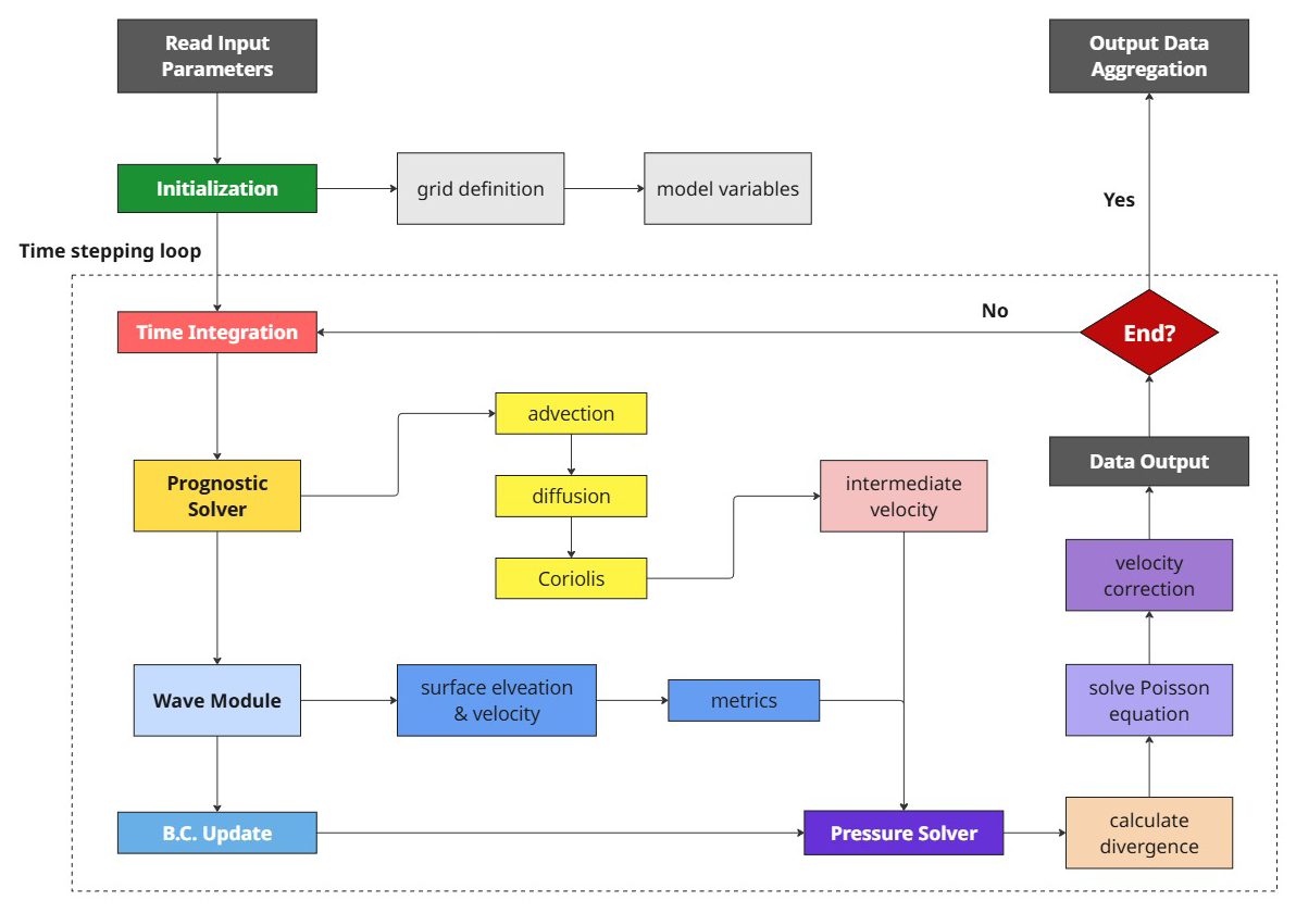
Within each time step, the model advances the solution through a structured time-stepping loop (Fig. 1). First, the prognostic solver computes the tendencies of the velocity components by integrating the momentum equations, i.e., Eqs. (10), (11), and (12), yielding an intermediate velocity field. Subsequently, the wave module updates the surface elevation and wave-induced velocities, from which the sigma-coordinate metrics are recalculated. Based on the updated wave information, the boundary conditions are then updated accordingly. The simulation then proceeds to the pressure solver stage, where the divergence of the intermediate velocity field is computed, the Poisson equation Eq. (25) is solved, and the velocity field is corrected to enforce the incompressibility constraint (Note that the pressure solver can be invoked immediately after model initialization to improve the divergence-free condition prior to time integration).

One iteration of the time-stepping loop is completed at this point. The solver continues looping through these steps until the prescribed simulation end time is reached. During the time-stepping procedure, simulation data are written at user-defined output intervals. After completion of the simulation, the output data are organized and aggregated into the final output files. For clarity, the main steps of the algorithm are summarized as follows:

1. Read input parameters and initialize the model.

2. Predict the intermediate velocity field using the prognostic equations.

3. Update the wave field and sigma coordinate metrics for boundary conditions and grid transformation.

4. Compute the velocity divergence and solve the pressure Poisson equation.

5. Correct the velocity field to satisfy the continuity constraint.

6. Collect flow statistics to temporary files.

7. Repeat steps 2–6 for each timestep until the simulation end time.

8. Aggregate and write simulation results in final output files.

5 Simulation setup

In this study, we designed four simulation cases under identical geostrophic wind conditions, with $U_{\mathrm{g}}=\mathrm{5}\mathrm{m}{\mathrm{s}}^{-\mathrm{1}}$, but with varying wave scenarios, specifically, a no-wave reference case (NW), a wind-following wave case (FW), a wind-opposing wave case (OW), and a steady (non-propagating) wave case (SW). In FW, OW, and SW, the wave parameters are identical: a wave amplitude of A=1.6 m and a wavelength of λ=100 m. Assuming linear deep-water wave theory, this corresponds to a wave period of T=8 s and a phase speed of $c=\mathrm{12.5}\mathrm{m}{\mathrm{s}}^{-\mathrm{1}}$. The only difference between FW and OW is the wave propagation direction relative to the wind. Neutral atmospheric stability is maintained by initializing a uniform potential temperature of 283 K from the surface up to z_i=600 m, topped by a 100 m-thick inversion layer characterized by a lapse rate of 3.5 K km⁻¹.

The computational grid employs a horizontal resolution of $\mathrm{\Delta }x=\mathrm{\Delta }y=\mathrm{3}/\mathrm{64}\mathit{\lambda }=\mathrm{4.6875}\mathrm{m}$. In the vertical direction, the grid spacing is uniform at 2 m from the surface up to 64 m height. Above this level, the grid spacing gradually expands with a constant stretching ratio of 1.025, reaching a maximum cell size of 16 m. The total grid consists of $\mathrm{256}\times \mathrm{256}\times \mathrm{128}$ cells, resulting in a domain size of $\mathrm{1200}\mathrm{m}\times \mathrm{1200}\mathrm{m}\times \mathrm{850}\mathrm{m}$. Periodic boundary conditions are applied in both horizontal directions.

The simulation timestep is dynamically adjusted to satisfy the Courant-Friedrichs-Lewy (CFL) condition, and it stabilizes at approximately $\mathrm{\Delta }t=T/\mathrm{12}$. Each simulation was integrated for a total of 20 h. The final hour of output was used for calculating time-averaged vertical profiles, while the last 30 min (corresponding to approximately 225 wave periods) were used to compute and visualize wave-phase-averaged fields, including wave-induced velocity components, pressure, and momentum fluxes.

6 Results

6.1 Flow field

Figure 2 shows the instantaneous fluctuations of the horizontal velocity at a height of $\mathit{\lambda }/\mathrm{5}$, highlighting the near-surface flow structures under different bottom boundary conditions. Figure 2a depicts the reference NW case, where elongated streamwise streaks characteristic of atmospheric boundary layer turbulence are evident. In contrast, Fig. 2b–d all exhibit distinct and highly organized wavy flow structures that reflect the imposed sinusoidal wave geometry. Among these cases, the wind-opposing wave (OW) scenario produces the most pronounced wave-induced fluctuations, which strongly modulate and dominate over the background turbulence. The wind-following wave (WF) case also shows prominent wavy structures, although their amplitude is slightly reduced compared to OW. The steady wave (SW) case presents weaker and less coherent wavy patterns, where wave-induced fluctuations coexist with and are partially masked by turbulent motions.

Figure 2 Instantaneous fluctuations of horizontal velocity in the x-y plane at a height of $\mathit{\lambda }/\mathrm{5}$ for four cases: (a) no wave (NW), (b) wind-following wave (WF), (c) wind-opposing wave (OW), (d) steady wave (SW). The black arrows represent the horizontal velocity vectors.

Figure 3 shows instantaneous snapshots of the vertical velocity fluctuations and vertical profiles of the variances of both horizontal and vertical velocity components, thereby providing both intuitive and quantitative insight into the turbulence structure under different surface-wave conditions. For NW and SW cases, the instantaneous fields exhibit relatively weak near-surface vertical motions, and the variance profiles indicate comparable turbulence intensities throughout most of the boundary layer. This suggests that the steady swell-shape surface in our case behaves similarly to a rough flat lower boundary, with turbulence predominantly generated by shear rather than surface-induced motions. In contrast, the moving-wave cases (b and c) display distinctly different behavior. In the wind-following wave case, coherent wave-induced vertical motions are clearly visible near the surface but decay rapidly with height. This is consistent with the variance profiles, which indicate a modest enhancement of velocity fluctuations confined to a height of approximately half a wavelength above the surface. Above this region, the turbulence becomes much weaker than in the reference case, until almost negligible above one wavelength height. The wind-opposing wave (OW) case exhibits the strongest response among all configurations. Instantaneous fields reveal intense and vertically extended fluctuations, and the corresponding variance profiles confirm a substantial increase in both u and w that persists throughout a large fraction of the boundary-layer depth. This indicates that wind-opposing waves significantly enhance turbulent mixing and promote the upward transport of wave-induced energy, leading to a pronounced modification of the turbulence structure across the entire ABL.

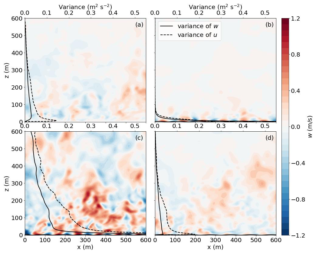
Figure 3 Instantaneous vertical velocity fluctuations w(x,z) (color shading) and vertical profiles of velocity variances for different surface-wave conditions. Solid and dashed black lines denote the variances of the vertical and streamwise velocity components, respectively, shown on the top x axis. Subplots (a)–(d) correspond to the NW, FW, OW, and SW cases.

As illustrated in Fig. 4, the presence of surface waves introduces pronounced oscillations in both the horizontal and vertical velocity components along the wave surface across all three cases. In the left column, the phase-averaged horizontal velocity 〈u〉 has distinct flow patterns depending on the wave condition.

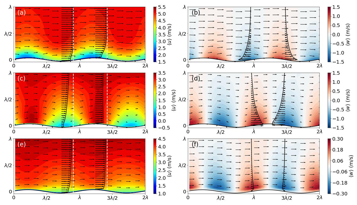
Figure 4 Phase-averaged velocity fields in the x–z plane. Left column: horizontal velocity component 〈u〉, with vertical profiles plotted above the wave troughs and crests. Right column: vertical velocity component 〈w〉, with vertical profiles plotted above the windward and leeward wave slopes. Subplots (a, b) correspond to the FW case, (c, d) to the OW case, and (e, f) to the SW case. Black arrows represent the phase-averaged velocity vectors and the white dashed lines indicate the magnitude of the geostrophic wind.

For the wind-following wave (FW) case, acceleration occurs above wave troughs, with the streamwise velocity quickly approaching the geostrophic wind speed (u_g) at approximately $z\approx \mathit{\lambda }/\mathrm{5}$. In contrast, deceleration is observed above the wave crests. The wind-opposing wave (OW) case exhibits the opposite behavior: flow deceleration above troughs and acceleration over crests. A similar spatial pattern is observed in the steady wave (SW) case, though with considerably reduced intensity, indicating weaker influences on the flow by fixed surface bumps.

In the right column, the vertical velocity 〈w〉 further highlights the impact of wave motion. For the FW case, upward motion is found above the leeward slopes, while downward motion appears above the windward sides. This behavior reverses in the OW and SW cases. The magnitude of 〈w〉 in the FW and OW cases is nearly an order of magnitude larger than in the SW case, underscoring the importance of wave propagation in enhancing vertical motion. The vertical profiles of 〈w〉 decay exponentially with height, becoming negligible above z≈λ, consistent with theoretical and observational expectations for wave-induced motions (Makin et al., 1995; Högström et al., 2015; Wu et al., 2018). The simulated wave-induced flow structures in Fig. 4 exhibit strong consistency with the LES results presented by Sullivan et al. (2008), with a detailed comparison given in Appendix C.

Figure 5 presents the phase-averaged pressure fields in the x-z plane, showing strong pressure gradients near the wave surface that diminish rapidly with height. Across all wave cases, regardless of wave direction or motion, the pressure exhibits a consistent spatial pattern: positive pressure zones are located in the wave troughs, while negative pressure zones occur above the wave crests. However, the magnitude of pressure variation varies significantly among cases. The OW case exhibits the strongest pressure fluctuations, followed by the FW case, where the peak amplitude is roughly half that of OW. The SW case shows much weaker pressure variation, approximately an order of magnitude smaller. The pressure profiles along the wave surface (bottom right panel) further reveal differences in the phase relationship between pressure and surface elevation. In the SW case, pressure fluctuations are nearly out-of-phase with the wave elevation, implying a symmetric pressure distribution around the wave crest and trough. Nevertheless, in the FW case, the pressure maximum is shifted upwind (toward the front face of the wave), occurring slightly upstream of the trough. Conversely, in the OW case, the pressure peak is displaced towards downstream of the trough. This asymmetry in pressure distribution correlates with the patterns of vertical velocity discussed in Fig. 4, where the upward motion and high pressure are concentrated on the front slope of the wave (the side facing wave propagation). Such asymmetric pressure patterns lead to the so-called form stress, which plays a critical role in modifying the vertical profiles of both mean wind speed and direction above the wave surface.

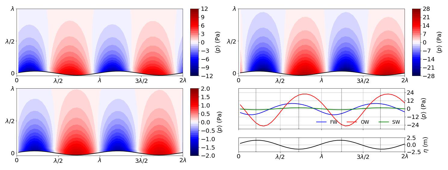
Figure 5 Phase-averaged pressure fields 〈p〉 in the x–z plane for the three wave scenarios: wind-following wave (FW, top left), wind-opposing wave (OW, top right), and steady wave (SW, bottom left). The bottom-right panel presents the corresponding pressure distributions along the wave surface (z=η) for all cases, plotted together for direct comparison, alongside the wave surface elevation η(x) in black. Dotted lines indicate the trough and crest positions.

6.2 Spectral characteristics

This section examines the spectral characteristics of the MABL flow under the influence of different wave conditions. The spectral analysis is based on velocity data collected from a 33×33 probe matrix with uniform horizontal spacing of 9.375 m, sampled at a frequency of 2 Hz over a duration of half an hour. Measurements were taken at multiple vertical levels to assess the height-dependent response of the flow.

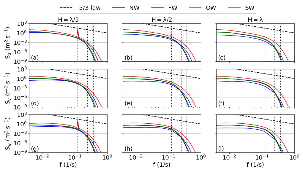
Figure 6 Horizontally averaged power spectral density curves of the three velocity components-u (top row), v (middle row), and w (bottom row), at three vertical heights: 20 m (left), 40 m (middle), and 100 m (right), under four different wave conditions (NW: no wave, FW: following wave, OW: opposing wave, SW: steady wave). The black dashed line indicates the $-\mathrm{5}/\mathrm{3}$ slope of the inertial subrange. Vertical dotted lines denote the wave frequency and its first two harmonics.

Figure 6 presents the power spectral density (PSD) curves of the three velocity components at three representative heights ($H=\mathit{\lambda }/\mathrm{5}$, $\mathit{\lambda }/\mathrm{2}$, and λ) for all wave cases. The impact of surface waves on the MABL flow manifests in two primary ways. First, in the u and w spectra, distinct peaks appear at the fundamental wave frequency and its first two harmonics below $H=\mathit{\lambda }/\mathrm{2}$. These spectral peaks indicate the presence of coherent wave-induced structures aligned with the direction of wave propagation. No such peaks are observed in the v component, suggesting that the wave effects are anisotropic and predominantly oriented in the streamwise and vertical directions. At H=λ, approximately one wavelength above the surface, these wave-induced signatures vanish, indicating limited vertical penetration of wave-coherent motions.

Second, surface waves substantially modify the overall turbulence energy distribution. Across all three velocity components and frequency bands, the opposing wave case exhibits significantly elevated PSD levels, indicating enhanced turbulence production throughout the boundary layer. In contrast, the FW case consistently exhibits reduced spectral energy, implying suppression of turbulence. These trends are not limited to the wave boundary layer (WBL) but extend across the entire vertical domain, consistent with the vertical profiles of turbulent kinetic energy (TKE) shown in Fig. 8f. Notably, the steady wave case yields PSD levels nearly identical to those observed over a flat surface, reinforcing the critical role of wave motion, rather than wave geometry alone, in shaping the boundary-layer turbulence dynamics.

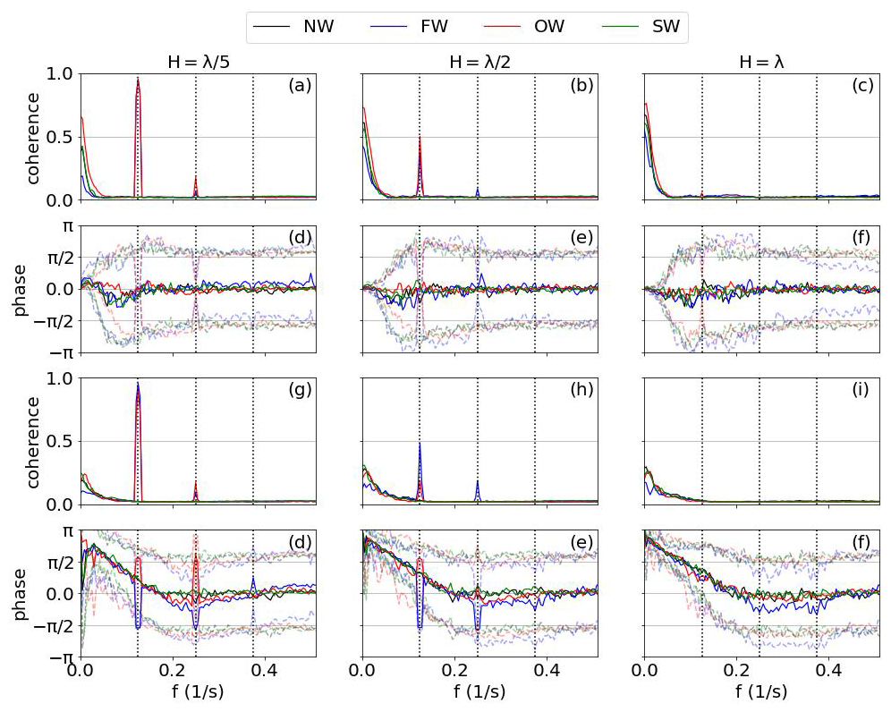
Figure 7 Vertical coherence and phase spectra for velocity components at a vertical separation of 20 m. The top two rows show the coherence and phase of the streamwise velocity (u–u), while the bottom two rows show the coherence and phase between streamwise and vertical velocity components (u–w). Each column corresponds to a different vertical location of the lower probe: $H=\mathit{\lambda }/\mathrm{5}$ (left), $H=\mathit{\lambda }/\mathrm{2}$ (middle), and H=λ (right). Black, blue, red, and green lines represent the NW, FW, OW, and SW cases, respectively. Dashed vertical lines indicate the wave fundamental frequency and its harmonics. The dashed lines in the phase spectra mark the ±1 standard deviation.

The power spectral density analysis indicates the presence of wave-induced temporal oscillations in the streamwise and vertical velocity components, especially below half a wavelength in height. To further investigate spatial coherent structures arising from wave motions, Fig. 7 presents vertical coherence and phase spectra between velocity components separated by 20 m. The first row displays the u-u coherence spectra. In the NW and SW cases, coherence decays exponentially with increasing frequency and vanishes beyond f≈0.05 Hz. In contrast, the FW and OW cases exhibit distinct coherence peaks approaching unity at the wave frequency when $H=\mathit{\lambda }/\mathrm{5}$. Peaks at the second harmonic are also observed, but with a weaker intensity. Interestingly, wave-induced coherence remains strong (up to 0.5) even at $H=\mathit{\lambda }/\mathrm{2}$, indicating that wave-induced coherent motions persist well above the surface layer. The corresponding phase spectra (second row) reveal minimal phase difference between u components at different vertical levels at wave-related frequencies. The standard deviation (dotted lines) increases sharply beyond f≈0.05 Hz, indicating loss of correlation and resulting in random phase differences. However, around the wave frequencies and harmonics, the phase variance collapses into an “hourglass” shape, further confirming the in-phase, vertically coherent structures induced by wave motion.

The third row shows u-w coherence, generally weaker in the low-frequency range than u-u, but exhibiting equally sharp peaks at wave frequencies in the FW and OW cases at $H=\mathit{\lambda }/\mathrm{5}$. Notably, at $H=\mathit{\lambda }/\mathrm{2}$, the FW case shows stronger wave-related coherence than the OW case. This implies that wave-induced u-w coupling becomes more prominent when the background turbulence is weaker. The bottom row presents u-w phase spectra. Unlike the in-phase behavior of u-u, the u-w phase shift exceeds $\mathit{\pi }/\mathrm{2}$ at low frequencies across all cases, suggesting that their product ($u^{\prime }{w}^{\prime }$) tends to fall into quadrant 2 and quadrant 4, corresponding to ejection and sweep events. This contributes to a negative vertical momentum flux. As frequency increases, the phase difference linearly decreases to zero around f≈0.2 Hz. Notably, the FW and OW cases show sharp $\pm \mathit{\pi }/\mathrm{2}$ phase shifts precisely at the wave frequency and harmonics, implying that wave-induced u-w structures are primarily out-of-phase, and thus do not significantly contribute to vertical turbulent momentum transport.

6.3 Vertical structure

We have previously discussed the characteristics of wave-induced velocity and pressure oscillations. These oscillations exert significant impacts on the vertical structure of MABL flows. First, surface waves contribute directly to the vertical momentum flux through the asymmetric pressure distribution along the wavy surface, as demonstrated in Fig. 5d. Specifically, the integral average of the horizontal pressure projection, expressed as

$$\begin{array}{}\text{(35)}& M_{\mathrm{w}}={\displaystyle \frac{\mathrm{1}}{\mathit{\lambda }}}\underset{\mathrm{0}}{\overset{\mathit{\lambda }}{\int }}p{\mathit{\zeta }}_x/{\mathit{\zeta }}_z\mathrm{d}x,\end{array}$$

acts effectively as a vertical momentum flux and can become the dominant dynamical forcing in the wave boundary layer. The velocity field is also strongly modulated by wave motions, but the streamwise and vertical wave-induced velocity components are predominantly out of phase, as shown in the last row of Fig. 7. As a result, their contribution to the momentum flux is negligible. Therefore, the total vertical momentum flux, here denoted as M, can be decomposed into two parts: the wave-induced momentum flux M_w and the turbulent momentum flux M_t. The first row of Fig. 8 presents their vertical profiles. In subplot (a), it is evident that M_w(z) decays exponentially with height in both the FW and OW cases. Remarkably, this decay is well described by the exponential function $f\left(z\right)=e^{-akz}$. The fitted decay coefficients are a=1.09 for the FW case and a=0.99 for the OW case, respectively. The fitted curves are plotted as dashed lines, but they are almost indistinguishable from the simulation results due to the excellent agreement. This provides strong support for the assumption of an exponential decay with a=1.0, adopted in our earlier parameterization study (Ning and Bakhoday-Paskyabi, 2025). The dashed lines indicate the estimated heights of the wave boundary layer in the two cases, defined as the levels where M_w decreases to 5 % of its surface value. These heights are both close to half the wavelength, with the WBL in the OW case extending slightly higher than in the FW case.

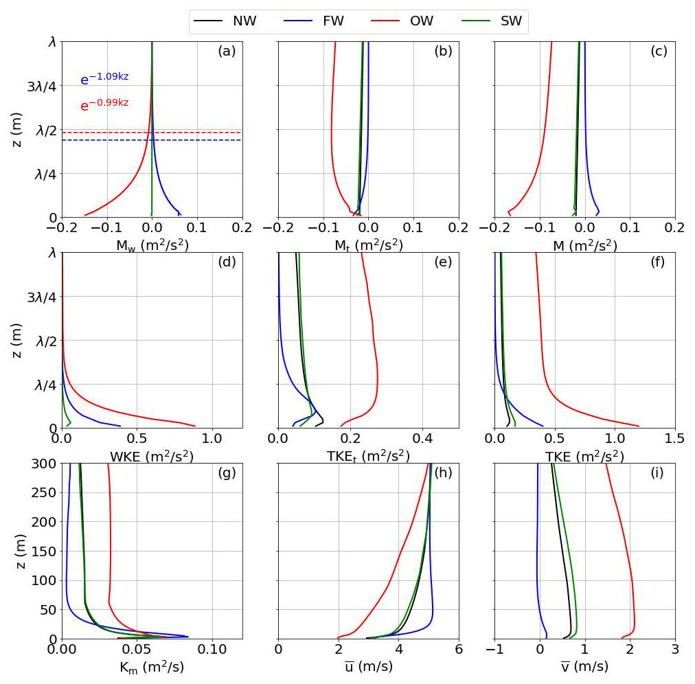
Figure 8 Vertical profiles of flow and turbulence statistics under different wave conditions. Top row: (a) Streamwise wave-induced momentum flux; (b) Turbulent momentum flux; (c) Total streamwise vertical momentum flux. Middle row: (d) wave-induced kinetic energy; (e) turbulent kinetic energy excluding wave contributions; (f) Turbulent kinetic energy. Bottom row: (g) Eddy diffusivity; (h) Mean streamwise velocity $\stackrel{\mathrm{‾}}{u}$; (i) Mean crosswise velocity $\stackrel{\mathrm{‾}}{v}$. Black, blue, red, and green curves represent the NW, FW, OW, and SW cases, respectively. In subplot (a), fitted exponential decay functions are also shown, along with markers indicating the heights where the wave-induced momentum flux decreases to 95 % of its surface value.

The turbulent momentum flux is also indirectly modulated by the presence of waves, as shown in subplot (b). Compared to the case with a flat surface (NW), M_t in the FW case is larger near the surface but decays rapidly to nearly zero by a height of $\mathit{\lambda }/\mathrm{4}$. This reduction is related to the much weaker wind shear over the wave boundary layer in the presence of following waves. In contrast, the OW case exhibits an enhancement of downward momentum flux throughout the boundary layer due to the additional surface drag imposed by the opposing wave. Figure 8c further illustrates that the influence of waves on the total vertical momentum flux extends well above the top of WBL. Additionally, the SW case, with a fixed wave surface, does not induce significant changes in the momentum flux profiles relative to the NW case.

Similarly, the total turbulent kinetic energy can be decomposed into the wave-induced kinetic energy (WKE) and the non-wave-related turbulent kinetic energy (TKE_t). Their vertical profiles are shown in the second row of Fig. 8 to illustrate the influence of waves on TKE. WKE, associated with wave-coherent flow motions, also exhibits an exponential decay with height. However, the decay rate is higher than that observed for the momentum flux, and its magnitude is highly sensitive to the relative orientation between the wind and wave directions rather than to the wave characteristics alone. Under the same wave amplitude and phase speed, WKE at the first grid level in the wind-opposing wave case (accounts for 73.8 % of TKE), is nearly twice as large as in the wind-following wave case, where WKE represents 97 % due to the much lower total energy level. By comparison, the case with a steady wavy surface shows a smaller contribution, with WKE comprising only about 20 % of TKE. The modification of TKE by waves further affects the parameterization of eddy diffusivity, as shown in Fig. 8g. The larger values of K_m in the OW case indicate stronger turbulent mixing of scalars and momentum, while in contrast, K_m in the FW case is nearly an order of magnitude smaller, reflecting a more stratified boundary layer structure. These trends are also evident in Fig. 3b.

Subplots (h) and (i) present the vertical profiles of the streamwise and crosswise velocity components, respectively. In the FW case, the streamwise velocity profile exhibits a pronounced knee-shaped turn at $z\approx \mathit{\lambda }/\mathrm{4}$, above which the wind becomes nearly uniform. This characteristic profile is commonly observed when low wind speeds are aligned with fast-propagating underlying waves (Högström et al., 2013). Conversely, in the OW case, the streamwise wind speed is substantially reduced from the surface up to 300 m, primarily due to surface drag increasing to nearly eight times that observed in the NW and SW cases. Although wave-coherent motions are confined to the x-z plane, the profile of v is strongly affected by waves. This occurs because changes in u alter the Coriolis force and reshape the Ekman spiral, thus resulting in a clockwise wind veer in the FW case and an anticlockwise rotation in the OW and SW cases relative to the case without waves.

6.4 Surface layer under wave impacts

The Monin-Obukhov Similarity Theory (MOST) has been widely employed to estimate the wind profile and stress within the surface layer and has shown good agreement with observations under a variety of conditions. Under neutral stratification, the wind profile predicted by MOST follows a logarithmic form:

$$\begin{array}{}\text{(36)}& \stackrel{\mathrm{‾}}{U}\left(z\right)={\displaystyle \frac{u_{*}}{\mathit{\kappa }}}\ln \left({\displaystyle \frac{z}{z_{\mathrm{0}}}}\right),\end{array}$$

where the friction velocity $u_{*}=\sqrt{\left|M\right|}$ is assumed constant. However, when wind-wave coupling is not in equilibrium, particularly in the presence of fast-moving swell beneath relatively low winds, as in our FW and OW cases, the Eq. (36) may no longer accurately represent the actual wind profile due to additional wave-induced flow contributions. Figure 9 compares the MOST-predicted logarithmic profiles to our simulation results, demonstrating the extent to which wave-dominated wind deviates from classical similarity theory.

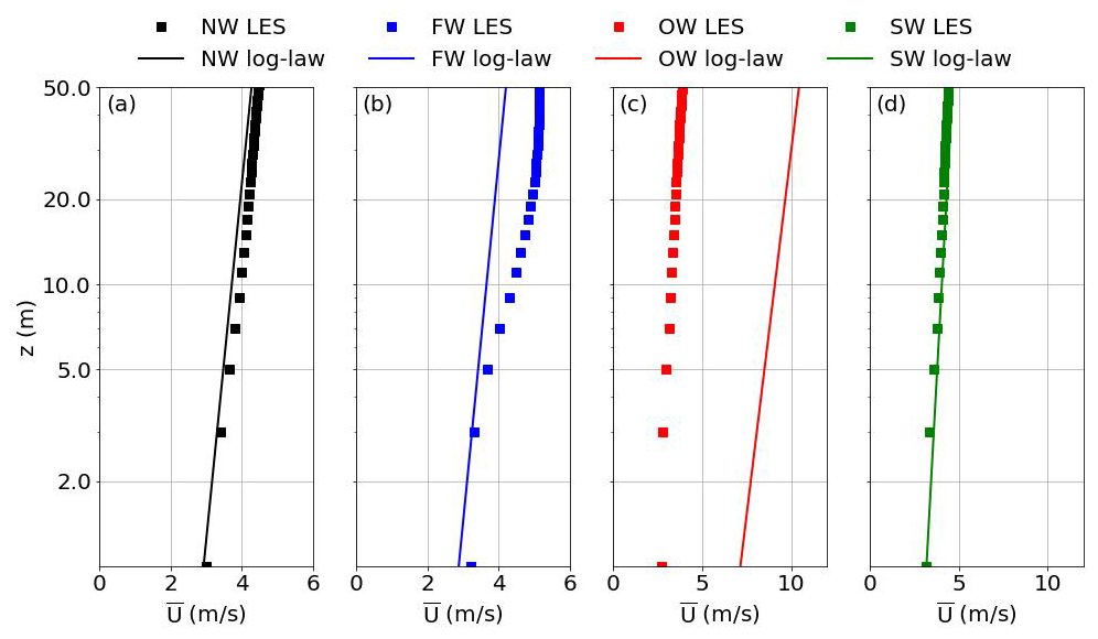
Figure 9 Comparison between the simulated mean wind speed profiles (by square markers) and the corresponding logarithmic wind profiles calculated by MOST (by solid lines) for each case: (a) NW, (b) FW, (c) OW, and (d) SW. The friction velocity used for MOST is derived from a 10 m height.

Here, the friction velocity is computed based on the momentum flux along the mean wind direction at the reference height z=10 m, i.e.

$$\begin{array}{}\text{(37)}& u_{*,\mathrm{10}}=\sqrt{{\displaystyle \frac{|{\mathit{M}}_{\mathrm{10}}\cdot {\stackrel{\mathrm{‾}}{\mathit{U}}}_{\mathrm{10}}|}{\left|{\stackrel{\mathrm{‾}}{\mathit{U}}}_{\mathrm{10}}\right|}}}.\end{array}$$

As expected, the wind profile in the NW case forms an approximately straight line on the logarithmic scale, closely following the log-law predicted by MOST. In contrast, substantial deviations appear in both the wind-following and wind-opposing wave cases. In the FW case, the wind speed begins to exceed the logarithmic profile just above 3 m, with the wave-driven component contributing 19.6 % more wind speed than the log-law prediction at 10 m height, reaching a maximum excess of 26.8 % at 23 m. Conversely, in the OW case, the log-law significantly over-predicts the near-surface wind: at the wave surface, it estimates wind speeds 1.6 times higher than those resolved in the simulation. The discrepancy further increases with height. In contrast, the SW case shows excellent agreement with the log-law until a height of 50 m, indicating that a steady wave field effectively behaves as a roughness element that can be effectively parameterized by an equivalent roughness length.

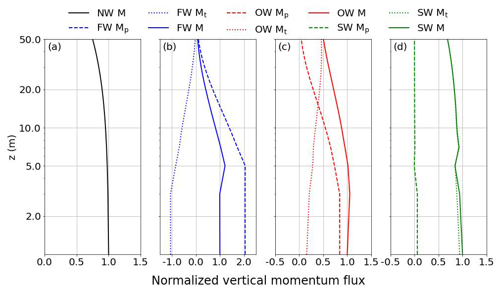
Figure 10 Vertical profiles of normalized momentum flux components in the four cases: (a) NW, (b) FW, (c) OW, and (d) SW. Solid lines denote the total vertical momentum flux, dashed lines show the wave-induced contribution, and dotted lines indicate the turbulent contribution. All fluxes are normalized by the surface momentum flux in each case.

Table 2 Surface layer parameters obtained from LES results.

An important premise of MOST is the assumption of a constant momentum flux within the surface layer. To evaluate the validity of this assumption under different wave conditions, Fig. 10 presents the vertical profiles of the partitioned momentum flux. Overall, the constant flux approximation holds reasonably well up to a height of 10 m in all cases, particularly for the case without waves. At 10 m, the total momentum flux remains at 81.7 %, 88.3 %, and 88.4 % of its surface value in the FW, OW, and SW cases, respectively. These results are consistent with the observations reported by Högström et al. (2013), and support the parameterization approaches proposed by Semedo et al. (2009), Wu et al. (2018), and Ning and Paskyabi (2024), where the wave-induced stress is incorporated into the log-wind formulation. However, it is evident that in both FW and OW cases, the momentum flux within the near-surface layer is strongly dominated by the wave-induced component. This dominance causes the total flux to decay substantially above 10 m, as the contribution from wave-induced stresses diminishes rapidly over this height.

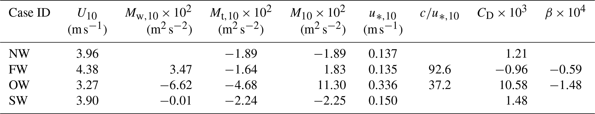
As the wave propagates beneath the wind, the energy exchange between wind and wave is done by the form stress generated from the pressure distribution along the wind-wave interface. The associated wave damping rate can be expressed as the product of this stress and the wave phase speed:

$$\begin{array}{}\text{(38)}& \mathit{\beta }=-{\displaystyle \frac{{\mathit{\tau }}_{\mathrm{w}}}{{\mathit{\rho }}_{\mathrm{w}}}}\cdot {\displaystyle \frac{\mathit{c}}{\frac{\mathrm{1}}{\mathrm{2}}g{A}^{\mathrm{2}}}}=-{\displaystyle \frac{\frac{{\mathit{\rho }}_a}{\mathit{\lambda }}{\int }_{\mathrm{0}}^{\mathit{\lambda }}p{\mathit{\zeta }}_x/{\mathit{\zeta }}_z\mathrm{d}x}{\frac{\mathrm{1}}{\mathrm{2}}{\mathit{\rho }}_{\mathrm{w}}\mathit{\omega }{A}^{\mathrm{2}}}}.\end{array}$$

Table 2 summarizes the wave damping rates computed for cases FW and OW, together with other key parameters characterizing the surface layer derived from the LES results.

The wave age $c/u_{*,\mathrm{10}}$ in both FW and OW cases greatly exceeds the threshold value of 20 (Cohen and Belcher, 1999), implying that they are clear wave-driven wind scenarios. Notably, the computed wave damping rates are on the order of 10⁻⁴, in good agreement with the fitted values reported by Semedo et al. (2009). Furthermore, despite identical background geostrophic wind and wave parameters, the damping rate β in case OW is approximately 2.5 times higher than in case FW, underscoring the strong dependence of wind-wave interaction on the relative alignment between wind and wave propagation. The wind-opposing wave configuration produces substantially stronger momentum and energy exchange across the interface, manifesting as enhanced surface drag, increased turbulence intensity, and a pronounced reduction in near-surface wind speeds. As a result, the drag coefficient C_D increases markedly from $\mathrm{1.21}\times {\mathrm{10}}^{-\mathrm{3}}$ in the NW case to $\mathrm{1.06}\times {\mathrm{10}}^{-\mathrm{2}}$ in OW, while in FW it is reduced to $-\mathrm{9.6}\times {\mathrm{10}}^{-\mathrm{4}}$, where the negative sign denotes an upward momentum flux from the waves to the atmosphere. These trends are qualitatively consistent with the LES findings reported by Jiang et al. (2016).

7 Conclusions

In this work, we developed a wave-phase-resolved large-eddy simulation solver employing a sigma coordinate system, implemented within the framework of the PALM model system, to investigate wind-wave interactions and their impacts on MABL flows. The newly implemented surface-following coordinate formulation enables direct resolution of the flow dynamics induced by the time-varying wavy surface geometry. To evaluate the model's performance, we configured four simulation cases, including a flat surface, wind-following waves, wind-opposing waves, and steady waves. Clear peaks observed in the power and coherence spectra demonstrate the presence of strong wave-coherent flow structures in the wave boundary layer. Moving waves also modify the vertical structure of the boundary layer by imposing momentum fluxes via the asymmetric pressure distributions along the wave surface. The magnitude and orientation of these fluxes are strongly dependent on the combined wind and wave conditions. Although the wave-induced velocity and pressure fluctuations decay exponentially with height and become negligible above approximately half a wavelength, their influence on the wind speed and turbulent kinetic energy profiles extends much farther into the boundary layer.

The solver successfully reproduces typical wave-driven flow features observed under low-wind conditions with strong swell and highlights the essential role of wave motion and propagation direction in shaping MABL dynamics. Further validation work is planned, including coupling the solver with advanced wave models to represent spectral wave fields and comparing the simulated results against observational data. In addition, investigating wave impacts under a broader range of wave age, wind-wave misalignment, and atmospheric stability conditions will be an important focus of future studies.

Since the sigma coordinate framework implemented in PALM-Sigma enables the simulation of turbulent flows over non-flat and moving surfaces, its potential applications are not limited to wind-wave interaction over the ocean but also extend to flows over complex terrain or other inhomogeneous topographic features. Overall, PALM-Sigma provides a high-fidelity modeling tool for atmosphere-wave coupled simulations, facilitating both fundamental investigations of wind-wave interaction processes and the evaluation and development of parameterization approaches.

Appendix A: Inertial oscillation

To assess the spin-up behavior and the influence of inertial oscillations, the temporal evolution of both the mean flow and the total kinetic energy is examined. Figure A1 shows the evolution of the horizontally averaged streamwise velocity profiles, $\stackrel{\mathrm{‾}}{u}$, over the 20 h simulation period for the different wave configurations. During the early stage of the simulations, pronounced inertial oscillations are visible, particularly within the lower boundary layer. As the simulations progress, the mean velocity profiles gradually converge toward a quasi-steady structure, with only weak residual oscillations remaining toward the end of the simulation.

In addition, Fig. A2 presents the temporal evolution of the domain-averaged total kinetic energy for the NW, FW, and OW cases. After an initial adjustment phase associated with inertial oscillations, the total kinetic energy in all cases approaches a statistically steady level and remains bounded without any trend of monotonic growth or decay. This behavior indicates that the dominant energy sources and sinks are in balance over long timescales and that no spurious numerical energy accumulation occurs. The statistical analyses presented in this study are therefore based on the last hour of the simulations, when the mean flow has largely adjusted, and inertial oscillations have substantially decayed.

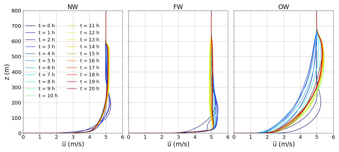
Figure A1 Temporal evolution of profiles of the horizontally averaged streamwise velocity, $\stackrel{\mathrm{‾}}{u}$, over the 20 h simulations for the different wave configurations. Case SW exhibits nearly identical behavior to Case NW and is therefore not shown.

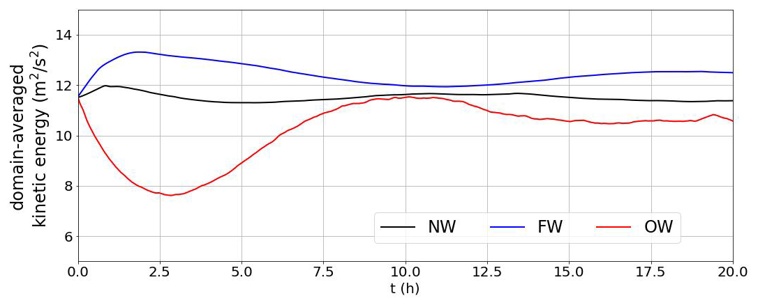
Figure A2 Temporal evolution of domain-averaged kinetic energy during the 20 h simulations for the NW, FW, and OW cases.

Appendix B: Sensitivity to vertical grid stretching within the atmospheric boundary layer

To assess the sensitivity of the simulated results to the application of vertical grid stretching within the atmospheric boundary layer, additional numerical experiments were conducted using a uniform vertical grid spacing. In these simulations, the vertical grid spacing was kept at a uniform value of 2 m in the z direction from the surface up to a height of 600 m, corresponding approximately to the top of the atmospheric boundary layer, while the same grid-stretching strategy as in the reference simulations was applied above this height. All other numerical settings, forcing conditions, and model parameters were kept identical to those of the original wind-following and wind-opposing wave cases.

Figure B1 compares the vertical profiles of the time-averaged horizontal velocity components $\stackrel{\mathrm{‾}}{u}$, $\stackrel{\mathrm{‾}}{v}$, and TKE between cases using vertically stretched grids (FW and OW) and uniform vertical grids (FW-UZ and OW-UZ). For both flow configurations, the mean velocity profiles show an excellent agreement throughout the boundary-layer depth, indicating a negligible sensitivity of the mean flow structure to the choice of vertical grid spacing. For the OW case, the uniform-grid simulation exhibits slightly reduced TKE values compared to the stretched-grid simulation, with a maximum absolute difference of approximately 0.08 m² s⁻², and this discrepancy gradually diminishes with increasing height. This behavior suggests that near-surface turbulence statistics under OW conditions may exhibit more sensitivity to vertical grid resolution than FW, which merits further investigation. Despite this moderate reduction in TKE, the overall vertical distribution of TKE and the associated turbulent characteristics remain similar between the two grid configurations.

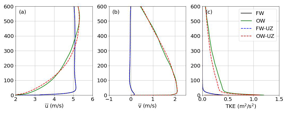
Figure B1 Vertical profiles of time-averaged horizontal velocity components $\stackrel{\mathrm{‾}}{u}$, $\stackrel{\mathrm{‾}}{v}$, and turbulent kinetic energy for wind-following (FW) and wind-opposing (OW) wave cases using vertically stretched grids (solid lines) and uniform vertical grids (dashed lines).

Appendix C: Comparison with previous wave-phase-resolved LES

Figure C1 compares vertical profiles of key flow statistics from the present simulations with corresponding results reported by Sullivan et al. (2008). Overall, the variance of the vertical velocity w, as in Fig. C1b, shows good agreement between the two studies across all cases, with a pronounced enhancement for the cases with moving waves (FW and OW) and negligible values for the SW case. This close agreement indicates that both solvers consistently capture wave-induced vertical motions, which are primarily governed by wave propagation and associated orbital motions rather than by the geometric shape of the wave surface alone.

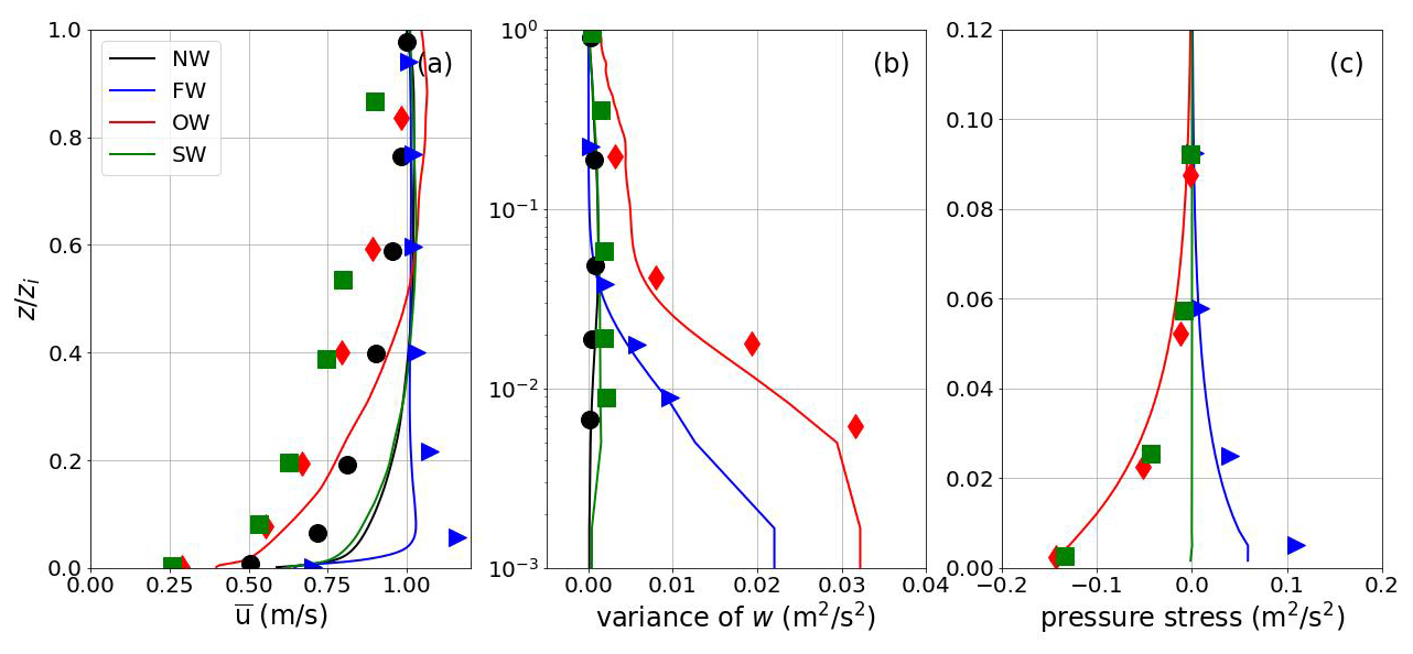
Figure C1 Comparison of vertical profiles of key flow statistics from the present study (solid lines) and Sullivan et al. (2008) (data points represented by markers) for (a) mean streamwise velocity, (b) variance of vertical velocity, and (c) wave-induced pressure stress, for the NW, FW, OW, and SW cases. Profiles are shown as a function of normalized height $z/z_i$.

In contrast, differences arise in the mean streamwise velocity profiles and the pressure-stress distributions. The discrepancies in $\stackrel{\mathrm{‾}}{u}$ are likely related to differences in the Coriolis parameter, determined by the geographical latitude, which controls the Ekman balance and can substantially influence the vertical structure of the mean flow even under similar geostrophic forcing. In addition, the different inversion-layer heights used in the two studies (600 m in the present simulations versus 400 m in Sullivan et al., 2008) may further affect momentum redistribution within the boundary layer.

Figure C1c implies that the remaining discrepancy between the OW and SW cases is mainly associated with differences in the wave-induced pressure contribution to the momentum flux. Our results imply that the absence of wave propagation and the associated surface particle motions substantially reduce the efficiency of pressure-modified momentum transfer under steady wave conditions. By comparison, Sullivan et al. (2008) reported a form drag for the SW case that is comparable in magnitude to that of the OW case, despite a much lower relative wind-wave speed. This difference reflects the model's sensitivity to the numerical discretization and the treatment of bottom boundary conditions, which can influence the representation of wave-induced pressure fields. Taken together, these contrasting results indicate that the mechanisms governing wave–pressure interaction over steady wave surfaces are not yet fully understood and would benefit from further targeted numerical intercomparisons and complementary experimental investigations.