Computation of fish larvae self-recruitment in using forward- and backward-in-time particle tracking in a Lagrangian model (SWIM-v2.0) of the simulated circulation of Lake Erie (AEM3D-v1.1.2)

Accurately estimating self-recruitment (SR), which is the fraction of recruits at a location that originated locally, is fundamental to understanding population connectivity. Biophysical models typically compute SR by releasing larval particles from source locations and tracking them forward in time. However, forward-tracking studies employ a variety of particle-release strategies (random, constant, area-scaled or production-scaled), which often leads to ambiguous SR estimates. Using theoretical analysis supported by numerical simulations of Lake Whitefish (Coregonus clupeaformis) larvae in Lake Erie, we show that SR is inherently dependent on larval production at all source locations. As a result, SR cannot be computed unambiguously in forward-tracking models unless the true larval production is known and released from every source location. In contrast, empirical parentage-analysis studies estimate SR directly as the fraction of locally produced juveniles among those sampled at a settlement location, without quantifying larval production at all sources. Motivated by this, we computed SR using backward-in-time particle tracking from the settlement location. We demonstrate that SR estimated using backtracking is independent of the number of particles released, which provides considerable benefit; namely the use of any magnitude of particles released and eliminating the need to identify all contributing sources or their larval output. This reduces the effort required to estimate SR and provides a theoretically consistent basis for its calculation. Our findings provide a theoretical framework for estimating SR and highlight the advantages of applying backtracking models for studying larval dispersal and recruitment.

1 Introduction

Self-recruitment (SR), local retention (LR), and relative local retention (RLR) are commonly used metrics to assess the tendency for self-maintenance of local populations (Botsford et al., 2009; Burgess et al., 2014; Cowen and Sponaugle, 2009; Lett et al., 2015; Hogan et al., 2012). Among these, SR [(locally produced settlement)$/$(settlement from all origins); Botsford et al., 2009] has been the most widely used descriptor of larval dispersal and is generally easier to measure experimentally (Burgess et al., 2014). However, LR [(locally produced settlement)$/$(total local larval release); Botsford et al., 2009] is strongly related to self-persistence or the ability of a population to sustain itself (Burgess et al., 2014; Lett et al., 2015; D'aloia et al., 2017); and RLR [(locally produced settlement)$/$(settlement originating from that location); Hogan et al., 2012; Lett et al., 2015] has gained recent attention because its denominator includes only successful dispersal events (Almany et al., 2017; Shi et al., 2024). Although these metrics share a common numerator (the number of locally produced settlers), their different denominators yield differences in their interpretation and calculation (see Sect. 2).

Typically, it is challenging to compute LR and RLR because it is difficult to measure the total number of eggs, larvae, or tracer particles produced at a source location for LR, or the total number of larvae that survive and successfully settle for RLR (Botsford et al., 2009; Lett et al., 2015; Burgess et al., 2014; Hogan et al., 2012). Consequently, biophysical models are usually coupled with forward-in-time Lagrangian particle-tracking models (hereafter “forward tracking models”) to estimate LR and RLR (Chaput et al., 2022; Saint-Amand et al., 2023; Sato et al., 2023; Gurdek-Bas et al., 2022; Karnauskas et al., 2022; Karnauskas et al., 2013). LR is then computed as the ratio of larvae that settle at their release location to the number initially released and RLR is similarly computed by excluding larvae that settle in unsuitable nursery habitats (Gurdek-Bas et al., 2022). Both LR and RLR are independent of the true larval production at the source location, which allows the release of a random number of simulated particles for their calculation, as demonstrated in this research.

In contrast, SR is generally easier to determine and has been studied more extensively (Lett et al., 2015; Burgess et al., 2014; D'aloia et al., 2013). For example, parentage analysis assigns sampled juveniles to their parents according to genetic markers, thereby identifying source locations and quantifying the number of locally produced settlers. SR has also been computed using biophysical models (Hiddink et al., 2013; Dubois et al., 2016; Klein et al., 2016; Faillettaz et al., 2018; Lequeux et al., 2018; Meerhoff et al., 2018; Hidalgo et al., 2019; Wolanski et al., 2021; Saint-Amand et al., 2023; Michie et al., 2024; Nadal et al., 2024; Corrochano-Fraile et al., 2022; Sato et al., 2023; Paris et al., 2005). In these models, larval particles are released from each source location and tracked forward in time, and SR is calculated as the number of particles that both originate from and settle at a given location divided by the total number of particles that settled there. A variety of particle-release strategies have been used, including: (1) releasing a random number of larvae (Sato et al., 2023); (2) releasing an equal number per location (Dubois et al., 2016; Faillettaz et al., 2018); (3) releasing larvae in proportion to habitat area (D'agostini et al., 2015); and (4) releasing larvae in proportion to estimated larval production (Nolasco et al., 2022). Notably, while the denominator (the total number of settlers at a location) reflects larval production from all potential sources, the numerator (the number of larvae both released from and settling at that location) depends on only the local larval production at the source. As a result, changes in larval production at any external source can alter the denominator while they cannot affect the numerator, and thereby influence SR estimates. This presents two challenges for forward-tracking approaches: identifying all possible source locations and determining the appropriate number of particles to release from each source. For these reasons, SR cannot be unambiguously computed using forward tracking models.

The objective of this research is to theoretically determine, in forward tracking simulations, whether LR and RLR and SR are independent of larval production at the source location. We examine the results of this endeavour and show that computing SR with a forward-tracking model produces ambiguous estimates regardless of the particle-release strategies. In contrast, we find that SR computed with a backtracking model informed by observations of Lake Whitefish (Coregonus clupeaformis) larvae collected in Lake Erie provide unambiguous results, i.e., it is independent of the number of recruits at the settlement location. We believe that these results are broadly applicable to both freshwater and marine species with pelagic larval phases.

2 Theoretical Development

2.1 Self-recruitment from forward tracking models

We introduce only the minimum mathematical notation required to compare forward- and backward-tracking formulations of SR for clarity. Suppose that there are n locations associated with larval hatching and subsequent settlement or recruitment (locations $\mathrm{1},\mathrm{2},\mathrm{\dots },i,j,\mathrm{\dots },n$). Let $N_i^{\prime }$ denote the number of eggs or newly hatched larvae produced at location i. After hatching, larvae enter a pelagic phase during which they are transported by water currents before settling. The dispersal rate from patch i to patch j, D_ij, is defined as the proportion of larvae released from location i that settle at location j. Because D_ij is defined as a proportion (i.e., a fraction of the total larvae released), it is inherently independent of $N_i^{\prime }$.

Local retention (LR) at location i, commonly computed in forward-tracking simulations (Saint-Amand et al., 2023; Sato et al., 2023), is defined following Shi et al. (2024):

$$\begin{array}{}\text{(1)}& {\text{LR}}_i={\displaystyle \frac{D_{ii}{N}_i^{\prime }}{N_i^{\prime }}}=D_{ii}.\end{array}$$

This result follows directly from the proportional nature of D_ij: the number of locally produced settlers scales linearly with $N_i^{\prime }$, and the scaling cancels in the ratio.

At the end of dispersal, some larvae settle at suitable nursery habitats, whereas others settle in unsuitable habitats and are considered “unsuccessful settlers” (Almany et al., 2017). Excluding the unsuccessful settlers from the denominator of LR yields relative local retention (RLR) (Hogan et al., 2012; Lett et al., 2015):

$$\begin{array}{}\text{(2)}& {\text{RLR}}_i={\displaystyle \frac{D_{ii}{N}_i^{\prime }}{{\sum }_{j=\mathrm{1}}^n{D}_{ij}{N}_i^{\prime }}}={\displaystyle \frac{D_{ii}}{{\sum }_{j=\mathrm{1}}^n{D}_{ij}}}.\end{array}$$

Here, ${\sum }_{j=\mathrm{1}}^n{D}_{ij}$ may be less than 1 because settlement in unsuitable habitats is excluded. As with LR, the proportional form of D_ij ensures that RLR is theoretically independent of $N_i^{\prime }$

Self-recruitment (SR = (locally produced settlement)$/$(settlement from all origins)) is given by (Botsford et al., 2009; Lett et al., 2015; Almany et al., 2017):

$$\begin{array}{}\text{(3)}& {\text{SR}}_i={\displaystyle \frac{D_{ii}{N}_i^{\prime }}{{\sum }_{j=\mathrm{1}}^n{D}_{ji}{N}_j^{\prime }}}.\end{array}$$

In this expression, the denominator depends on larval production at all source locations ($N_{\mathrm{1}}^{\prime },N_{\mathrm{2}}^{\prime },\mathrm{\dots },N_n^{\prime }$), not just location i. Therefore, SR is inherently sensitive to spatial variation in larval production. Any change in larval output at any other source location modified the total number of settlers arriving at i, and thus alters SR, even when local retention at i remains unchanged.

Although SR is often described informally as “the probability that a source location equals a settlement location”, Eq. (3) provides a formal expression for that probability. A central finding of this study is that this probability becomes dependent on larval production when computed with forward tracking, whereas backtracking yields a production-independent estimate.

If larval production is artificially assumed to be identical at all source locations (i.e., $N_{\mathrm{1}}^{\prime }=\mathrm{\dots }=N_n^{\prime }$), then SR simplifies to:

$$\begin{array}{}\text{(4)}& {\text{SR}}_i={\displaystyle \frac{D_{ii}}{{\sum }_{j=\mathrm{1}}^n{D}_{ji}}}.\end{array}$$

This expression resembles both LR and RLR in being independent of $N_i^{\prime }$, but it is only valid under the restrictive and often unrealistic assumption of uniform larval production. When larval production varies across locations, Eq. (3) must be used, and substantial discrepancies between Eqs. (3) and (4) can arise – especially when many source locations contribute recruits. Because LR and RLR depend only on dispersal proportions D_ij, their values can be computed unambiguously in forward-tracking models using any sufficiently large number of simulated particles released from each source. Releasing an arbitrary (random) number of particles N_i is acceptable because the proportional structure of D_ij ensures convergence as particle number increases. As noted by Shi et al. (2024), LR provides a minimum bound for RLR because LR includes both successful and unsuccessful settlers in the denominator.

In contrast, SR cannot be uniquely determined from a forward-tracking simulation unless the true larval production values $N_j^{\prime }$ at all source locations are known and used. Without this information, any particle-release strategy (equal numbers, area-weighted numbers, proportional to habitat, random, etc.) yields SR values that reflect the assumed production pattern rather than the true biological quantity. Thus, forward-tracking models cannot generally compute SR unambiguously unless realistic production values at all source locations are available.

2.2 Self-recruitment from backward tracking models

An alternative to forward tracking is to release larval particles from settlement locations (i.e., where larvae are recruited into the population) and track them backward-in-time to identify their origins. Suppose there are m settlement and hatching locations ($\mathrm{1},\mathrm{2},\mathrm{\dots },i,j,\mathrm{\dots },m$). Let $M_i^{\prime }$ be the true number of larvae recruited at settlement location i. The recruitment rate $R_{ij}^{\prime }$ is defined as the proportion of recruits at location i that originated from source location j. Self-recruitment (SR) at location i is then:

$$\begin{array}{}\text{(5)}& {\text{SR}}_i={\displaystyle \frac{R_{ii}^{\prime }{M}_i^{\prime }}{M_i^{\prime }}}=R_{ii}^{\prime }.\end{array}$$

Thus, SR is theoretically identical to the recruitment rate from the local source, and is independent of the number of recruits at that location. This property is biologically intuitive: in parentage-analysis studies, it is rarely possible to sample all recruits in the field, yet SR is consistently estimated as the fraction of sampled juveniles assigned to local parents (D'aloia et al., 2013; Almany et al., 2017). Even when only a subset of recruits is sampled, this ratio provides an unbiased estimate of SR, reinforcing that SR depends on the proportion of local recruits, not the absolute number.

In backtracking simulations, a random number of larval particles M_i is typically released from settlement location i. By the end of the simulation, some particles will trace back to suitable source locations, while others will terminate in unsuitable ones; the latter constitute “unreal” recruits (Shi et al., 2024). The settlement rate R_ij, is defined as the ratio of the number of larval particles that settle at location j and originate from location i, divided by the total number of larval particles released from location i. The difference between R_ij and $R_{ij}^{\prime }$ lies in the denominator: the former normalizes by M_i whereas the latter normalizes by the true number of recruits $M_i^{\prime }$, respectively.

If R_ij and M_i are substituted into Eq. (5), the result is not SR, but rather the imaginary self-recruitment (ISR), which is (Shi et al., 2024):

$$\begin{array}{}\text{(6)}& {\text{ISR}}_i={\displaystyle \frac{R_{ii}{M}_i}{M_i}}=R_{ii}.\end{array}$$

ISR represents a minimum bound on SR, as its denominator includes unreal recruits in addition to real ones. To obtain SR from a backward-tracking simulation, unreal recruits must be excluded from the denominator of ISR. This yields:

$$\begin{array}{}\text{(7)}& {\text{SR}}_i={\displaystyle \frac{R_{ii}{M}_i}{{\sum }_{j=\mathrm{1}}^n{R}_{ij}{M}_i}}={\displaystyle \frac{R_{ii}}{{\sum }_{j=\mathrm{1}}^n{R}_{ij}}}.\end{array}$$

As Eq. (7) shows, SR computed by backward tracking is theoretically independent of the number of larval particles released from location i. This independence arises because increasing or decreasing M_i rescales the numerator and denominator equally; the settlement rates R_ij remain unchanged. This is confirmed in the numerical examples presented later. Consequently, a random number of particles can be released from the settling location without impacting SR.

The relative local retention (RLR) at location i in backward-tracking simulations is:

$$\begin{array}{}\text{(8)}& {\text{RLR}}_i={\displaystyle \frac{R_{ii}{M}_i}{{\sum }_{j=\mathrm{1}}^n{R}_{ji}{M}_j}}.\end{array}$$

Unlike forward tracking (Eq. 2), RLR derived from backward tracking depends on the number of particles released from each location (M_i). This is expected because backward tracking does not redistribute particles across all source locations in proportion to their true production. Finally, backward tracking cannot compute LR because unsuccessful dispersal does not occur in backward time, just as forward tracking cannot compute ISR because unreal recruitment cannot occur in forward time.

2.3 Number of larvae produced and recruited at each location

The number of larvae produced at each source location $N_j^{\prime }$ may be computed for use in forward-tracking simulations to obtain unbiased estimates of SR. This can be inferred from the number of recruits observed at settlement locations, $M_i^{\prime }$, together with the recruitment matrix estimated from backward tracking simulations.

Consider a backward-tracking simulation in which M_i particles are released from settlement location I, of these, $M_i\cdot {\sum }_{k=\mathrm{1}}^n{R}_{ik}$ particles trace back to real (suitable) hatching locations, and $M_i\cdot (\mathrm{1}-{\sum }_{k=\mathrm{1}}^n{R}_{ik})$ trace back to unreal (unsuitable) locations. To ensure that the number of real recruits, in the simulation, matches the observed number or real recruits $M_i^{\prime }$ at settlement location i, the following must hold $M_i\cdot {\sum }_{k=\mathrm{1}}^n{R}_{ik}=M_i^{\prime }$. Thus, the number of particles released from location i in a backward-tracking simulation is $M_i=M_i^{\prime }/{\sum }_{k=\mathrm{1}}^n{R}_{ik}$. The number of recruits at location i that originated from source location j is therefore:

$$\begin{array}{}\text{(9)}& N_{ji}^{\prime }=R_{ij}\cdot M_i=M_i^{\prime }{\displaystyle \frac{R_{ij}}{{\sum }_{k=\mathrm{1}}^n{R}_{ik}}}\end{array}$$

From the dispersal rate D_ji (the proportion of larvae released at j that settle at i), the total larval production at source location j is:

$$\begin{array}{}\text{(10)}& N_j^{\prime }={\displaystyle \frac{N_{ji}^{\prime }}{D_{ji}}}=M_i^{\prime }\cdot {\displaystyle \frac{R_{ij}}{D_{ji}}}\cdot {\displaystyle \frac{\mathrm{1}}{{\sum }_{k=\mathrm{1}}^n{R}_{ik}}}.\end{array}$$

Interestingly, if we instead use the number of recruits observed at a different settlement location a (denoted is $M_a^{\prime }$), an equivalent expression for $N_j^{\prime }$ is obtained:

$$\begin{array}{}\text{(11)}& N_j^{\prime }=M_a^{\prime }\cdot {\displaystyle \frac{R_{aj}}{D_{ja}}}\cdot {\displaystyle \frac{\mathrm{1}}{{\sum }_{k=\mathrm{1}}^n{R}_{ak}}}.\end{array}$$

Equations (10) and (11) must agree for all recruitment locations i and a where both R_ij and R_aj are non-zero. Equating Eqs. (10) and (11) we obtain the number of recruits at location a as:

$$\begin{array}{}\text{(12)}& M_a^{\prime }=M_i^{\prime }\cdot {\displaystyle \frac{R_{ij}}{D_{ji}}}\cdot {\displaystyle \frac{D_{ja}}{R_{aj}}}\cdot \sum _{k=\mathrm{1}}^n{\displaystyle \frac{R_{ak}}{R_{ik}}}.\end{array}$$

This expression provides a constraint linking the number of recruits at different settlement locations. Both $N_j^{\prime }$ and $M_a^{\prime }$ are undefined when the dispersal, recruitment or settlement rates become zero. This reflects the fact that a location's production cannot be inferred from recruitment locations to which it contributes zero larvae, and vice versa.

3 Putting Theory into Practice: Application to Lake Erie

3.1 Study area

Shi et al. (2024) identified the principal Lake Whitefish larval hatching locations in Lake Erie using backward-tracking simulations. The locations were concentrated along the western and southern flanks of the western basin. Considering that Lake Whitefish spawn on hard substrates (Amidon et al., 2021), we selected four regions containing suitable substrate along these flanks as potential hatching locations (Fig. 1). These regions served as larval-release areas in our forward-tracking simulations. We refer to them as: Detroit River Mouth (region A), Western Shoreline (region B), Midlake Reefs (region C), and Bass Islands (region D) (Fig. 1c). The Midlake Reef and Bass Islands regions were also selected as settlement locations, from which larval particles were released in backward-tracking simulations. In this study, “settlement locations” refer specifically to regions C and D, identified in Shi et al. (2024) as primary juvenile collection zones based on empirical larval surveys.

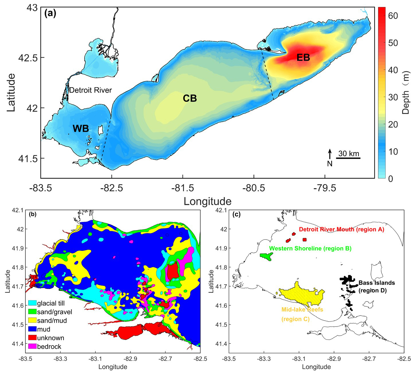
Figure 1 (a) Map showing the three basins of Lake Erie: western basin (WB), central basin (CB), and eastern basin (EB). The lake bathymetry was obtained from https://www.ngdc.noaa.gov/mgg/greatlakes/erie.html (last access: 22 January 2026). (b) Substrate distributions in the western basin from side-scan sonar transects (Haltuch et al., 2000). (c) Color coded Lake Whitefish (Coregonus clupeaformis) hatching locations (Detroit River Mouth in red, region A; Western Shoreline in green, region B; Mid-Lake Reefs in yellow, region C; Bass Islands in black, region D), where larval particles were released at the centre of each 500 m×500 m AEM3D grid (black cross-hatching).

3.2 The hydrodynamic model

Larval particle transport was driven by output from a hydrostatic three-dimensional Reynolds-averaged Navier–Stokes hydrodynamic model, the Aquatic Ecosystem Model (AEM3D) (HydroNumerics; https://www.hydronumerics.com.au, last access: 22 January 2026). AEM3D was applied in a continuous hindcast for 2017–2019 resolving water temperature and currents on a 500 m×500 m horizontal grid with 45 vertical layers (Shi et al., 2024; Lin et al., 2022). Vertical resolution was finest (0.5 m) through the surface layer, metalimnion, and near the bottom of the central basin, and coarser (5 m) in the deep hypolimnion of the eastern basin.

The model was forced with surface meteorological inputs (wind speed and direction, air temperature, relative humidity and long- and short-wave solar radiation) from four regional weather stations. Hydrological boundary conditions consisted of five major inflows (Detroit, Maumee, Sandusky, Cuyahoga and Grand rivers) and the Niagara River outflow.

AEM3D and its non-parallel predecessor, the Estuary and Lake Computer Model (ELCOM), have been extensively applied to Lake Erie. Previous applications include: backtracking Lake Whitefish larvae to determine hatching locations (Shi et al., 2024); hindcasting thermal structure (León et al., 2005); simulating internal wave dynamics (Valipour et al., 2015); surface wave and sediment transport modelling (Lin et al., 2021); simulating nutrient and chlorophyll-a distributions (Leon et al., 2011); modelling seasonal phytoplankton succession (Wang et al., 2024); forecasting storm surge and upwelling/downwelling events (Lin et al., 2022). These prior validation studies support the suitability of AEM3D for simulating larval dispersal processes in Lake Erie. Our model calibration and validation are published in the supplemental material of Shi et al. (2024). Briefly, in the western basin the mean modeled root-mean-square error (RMSE) was 0.99 °C during calibration (2018) and <2 °C during validation (2017–2019). These are consistent with a previous ELCOM calibration RSME of 0.9 °C in the western basin for 2008 (Liu et al., 2014). The model reproduced the timing and magnitude of the current fluctuations (∼10–20 cm s⁻¹) driven by the 14 h surface seiche (Boegman et al., 2001) with modeled RMSE of 2.9–3.2 cm s⁻¹. These are comparable to published applications of ELCOM, giving RMSE of 4.3–4.4 cm s⁻¹ in the central basin of Lake Erie (Lin et al., 2021). Model error in predicting mean current fluctuations was <10 % of measured values.

3.3 The Lagrangian particle tracking model

We used a Matlab^®-based Lagrangian particle tracking model (SWIM-v2.0) to study SR. Earlier versions of SWIM have been applied both forward-in-time to simulate silver eel (Anguilla rostrata and A. anguilla) migration (Béguer-Pon et al., 2016) and backward-in-time to identify Lake Whitefish hatching locations (Shi et al., 2024). Biological behaviours, such as diel vertical migration and active swimming, were not included consistent with previous Lake Whitefish studies (Di Stefano et al., 2022; Rowe et al., 2022; Suca et al., 2022).

A horizontal turbulent diffusivity $K_{\mathrm{h}}=\mathrm{0.1}{\mathrm{m}}^{\mathrm{2}}{\mathrm{s}}^{-\mathrm{1}}$ (Okubo, 1971) and timestep dt_p=600 s were used for both forward- and backward-tracking simulations. Larval particles were released at 3 m depth and removed upon intersecting the lake boundary (Shi et al., 2024). A uniform release depth of 3 m was used to maintain consistency between forward and backward tracking. This depth approximates the mixed-layer habitat typically occupied by early-stage Lake Whitefish larvae.

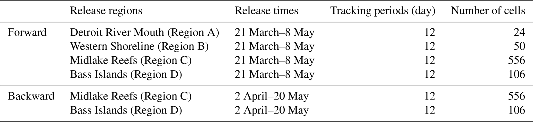
Forward-tracking particle releases occurred daily at 12:00 LT (noon) between 21 March and 8 May 2018, across four regions (A–D; Table A1). Releases were repeated at 7 intervals (every 8 d) and were tracked for 12 d, corresponding to the pelagic larval duration of Lake Whitefish (Shi et al., 2024). Backward-tracking releases occurred daily at 12:00 LT (noon) between 2 April and 20 May 2018, and particles were tracked for 12 d. Preliminary back-tracking tests from regions A and B showed negligible settlement in any of the four regions (A, B, C and D). To avoid unnecessary computational expense, we thus restricted backward releases to Regions C and D, which represent the principal settlement regions in Shi et al. (2024).

To examine how the number of released particles influences SR, we conducted simulations with three release magnitudes per region (Tables 1 and 2). Release regions were subdivided into 500 m×500 m AEM3D grid cells, and particles were released at cell centers. Since the number of cells varies by region (e.g., region A: 24 cells; region B: 50 cells, Table A1), we scaled particles per cell to keep the total releases consistent within each scenario. In region A, we released 100, 500, 900 particles per cell, giving 16 800, 84 000 and 151 200 particles per simulation (e.g., $\mathrm{100}\mathrm{particles}{\mathrm{cell}}^{-\mathrm{1}}{\mathrm{time}}^{-\mathrm{1}}\times \mathrm{24}\mathrm{cells}\times \text{7 times}=\mathrm{16}\mathrm{800}\mathrm{particles}$). In region B, we released 50, 200, 400 particles per cell, giving 17 500, 70 000 and 140 000 particles per simulation (e.g., $\mathrm{50}\mathrm{particles}{\mathrm{cell}}^{-\mathrm{1}}{\mathrm{time}}^{-\mathrm{1}}\times \mathrm{50}\mathrm{cells}\times \text{7 times}=\mathrm{17}\mathrm{500}\mathrm{particles}$). Regions C and D were also partitioned in the same manner for consistency.

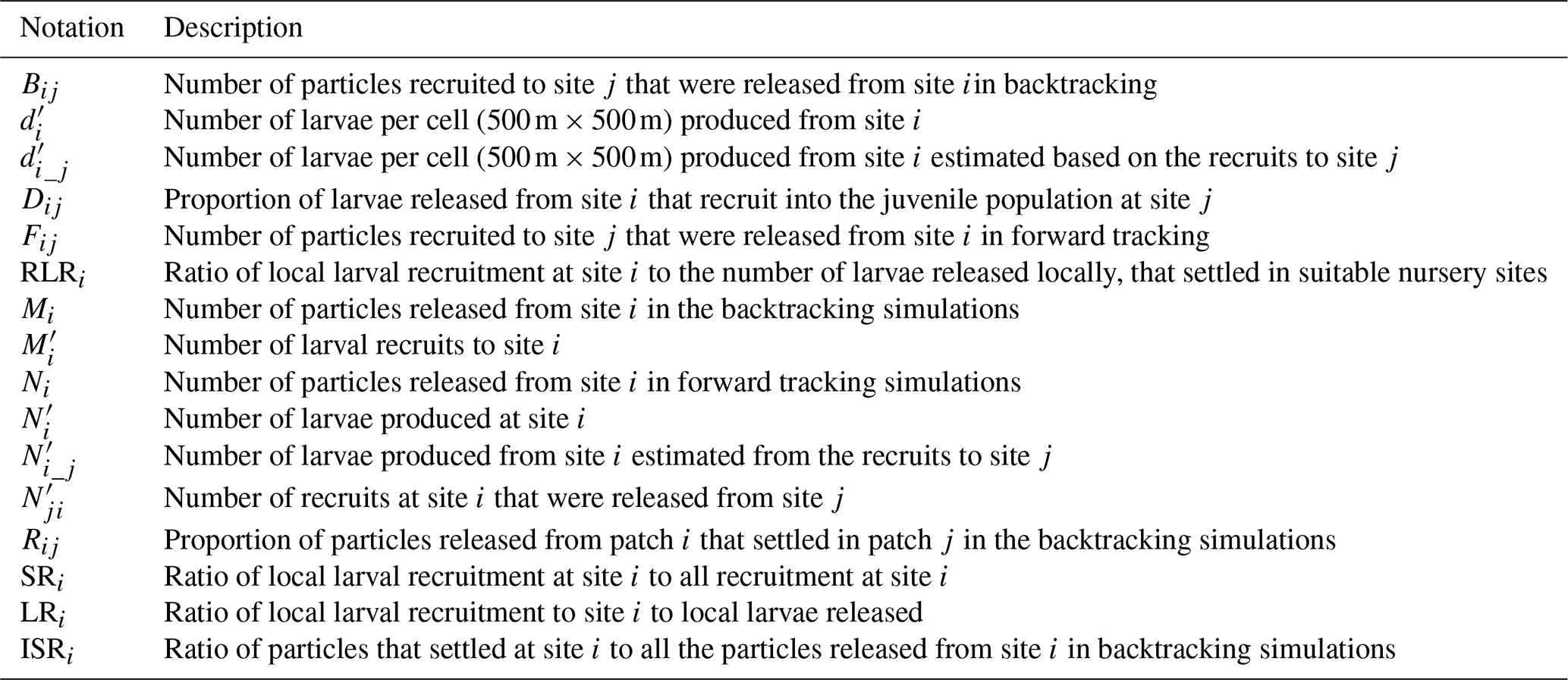
3.4 Nomenclature and data analysis

To clarify the variables used in our analysis, here we define the notation, and summarize all variable definitions in Table A2. In the forward-tracking simulations, N_i particles were released from each location i, with F_ij being the number that arrived at each destination j. For example, if N_A particles were released from region A, then F_AC particles settled in region C. In backward-tracking simulations, M_i particles were released from each location i, with B_ij being the number that traced back to location j. For example, if M_C particles were released from region C, then B_CA particles backtracked to region A, corresponding to recruits at C that originated from A.

The corresponding dispersal and recruitment (settlement) rates are:

$$\begin{array}{}\text{(13)}& {\displaystyle }& {\displaystyle }{D}_{ij}={\displaystyle \frac{F_{ij}}{N_i}},\text{(14)}& {\displaystyle }& {\displaystyle }{R}_{ij}={\displaystyle \frac{B_{ij}}{M_i}}.\end{array}$$

From Sect. 2.3, estimating the true larval production at location j requires information from both forward-tracking dispersal rates and backward-tracking recruitment rates, along with the number of real recruits. In general, this is given by:

$$\begin{array}{}\text{(15)}& \begin{array}{rl}{\displaystyle }{N}_j^{\prime }={\displaystyle \frac{N_{ji}^{\prime }}{D_{ji}}}& {\displaystyle }=M_i^{\prime }\cdot {\displaystyle \frac{R_{ij}}{D_{ji}}}\cdot {\displaystyle \frac{\mathrm{1}}{{\sum }_{k=\mathrm{1}}^n{R}_{ik}}}\\ {\displaystyle }& {\displaystyle }=N_j{\displaystyle \frac{M_i^{\prime }}{M_i}}\cdot {\displaystyle \frac{B_{ij}}{F_{ji}}}\cdot {\displaystyle \frac{\mathrm{1}}{{\sum }_{k=\mathrm{1}}^n{R}_{ik}}},\end{array}\end{array}$$

where forward- and backward-tracking quantities link larval release, settlement and recruitment.

Because only regions C and D were used as backward-tracking release locations in this study, larval production at location j is expressed as $N_{j\mathit{\_}\mathrm{C}}^{\prime }$ or $N_{j\mathit{\_}\mathrm{D}}^{\prime }$:

$$\begin{array}{}\text{(16)}& {\displaystyle }& {\displaystyle }{N}_{j\mathit{\_}\mathrm{C}}^{\prime }=N_j{\displaystyle \frac{M_{\mathrm{C}}^{\prime }}{M_{\mathrm{C}}}}\cdot {\displaystyle \frac{B_{\mathrm{C}j}}{F_{\text{jC}}}}\cdot {\displaystyle \frac{\mathrm{1}}{{\sum }_{k=\mathrm{1}}^n{R}_{\mathrm{C}k}}},\text{(17)}& {\displaystyle }& {\displaystyle }{N}_{j\mathit{\_}D}^{\prime }=N_j{\displaystyle \frac{M_{\mathrm{D}}^{\prime }}{M_{\mathrm{D}}}}\cdot {\displaystyle \frac{B_{\mathrm{D}j}}{F_{\text{jD}}}}\cdot {\displaystyle \frac{\mathrm{1}}{{\sum }_{k=\mathrm{1}}^n{R}_{\mathrm{D}k}}}.\end{array}$$

For example, $N_{\mathrm{A}}^{\prime }$ is the number of larvae produced from region A. To estimate $N_{\mathrm{A}}^{\prime }$, requires both backward and forward tracking simulations, and the number of recruits to a given location. Here, we only backtracked particles from region C and D; therefore, $N_{\mathrm{A}}^{\prime }$ can be computed using the recruits at region C or D ($M_{\mathrm{C}}^{\prime }$ or $M_{\mathrm{D}}^{\prime }$) and is denoted as $N_{\mathrm{A}\mathit{\_}\mathrm{C}}^{\prime }$ or $N_{\mathrm{A}\mathit{\_}\mathrm{D}}^{\prime }$, respectively. Dividing $N_{\mathrm{A}\mathit{\_}\mathrm{C}}^{\prime }$ by the number of AEM3D grid cells in region A (or the total area of the 500 m×500 m grid cells) gives the density $d_{\mathrm{A}\mathit{\_}\mathrm{C}}^{\prime }$.

4 Results

4.1 Larval distribution patterns

Most particles backtracked to regions west of their release locations, with relatively few tracing eastward (Fig. 2), consistent with the predominant west-to-east circulation in western Lake Erie (Beletsky et al., 2013). The exception was region A, where local circulation patterns were more variable. When particles were released from settlement region C and tracked backward for 12 d, they predominantly traced to the southern and western franks of the western basin (golden circles in Fig. 2c). These backtracking results agree with the modeled Lake Whitefish hatching locations reported by Shi et al. (2024), where larvae were sampled close to region C.

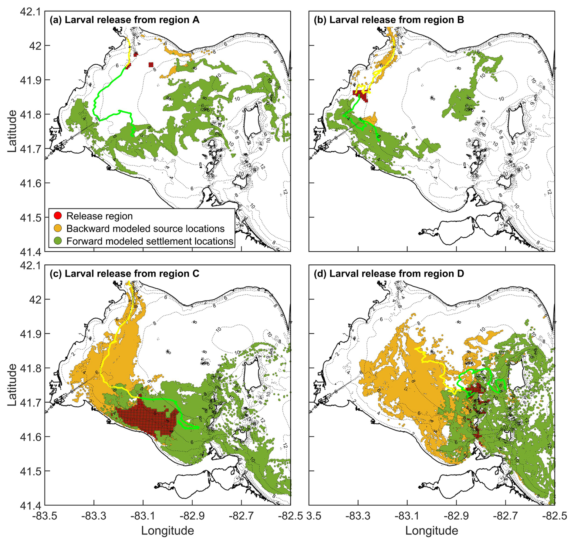
Figure 2 Modelled source location distributions (gold circles; backtracking) and settlement locations (dark green circle; forward tracking) for particles released from (a) region A, (b) region B, (c) region C, and (d) region D. Particles were tracked for 12 d in both forward and backward simulations. In backward tracking, the release region represents settlement location; in forward tracking, it represents the source location. The fraction of particles returning to their release region indicates imaginary self-recruitment (backtracking) or local retention (forward tracking). The ratio of particles returning to their release region, to the total settling in all four regions, indicates self-recruitment (backtracking). Yellow/green line shows example backward/forward trajectories.

Forward-tracking simulations showed the opposite pattern: particles released from each of the four regions were generally transported eastward over the 12 d tracking period (dark green circles in Fig. 2), again matching the prevailing flow direction in the lake. An exception occurs Fig. 2b, where some particles move southeast or northeast of the release region. Although counter-intuitive, relative to the dominant flow, such deviations are reasonable given the complex bathymetry and variable wind-field in the western basin.

It is known that dispersal estimates are sensitive to the number of particles released (Béguer-Pon et al., 2016); therefore, we conducted a sensitivity analysis. When too few particles were released, dispersal patterns fluctuated markedly (Fig. 3). However, the results show that the estimated dispersal rate, local retention (Eq. 2) and self-recruitment all become invariant when more than 40 000 particles were released in both forward- and backward-tracking simulations (Fig. 3). This threshold was used to ensure statistically robust results.

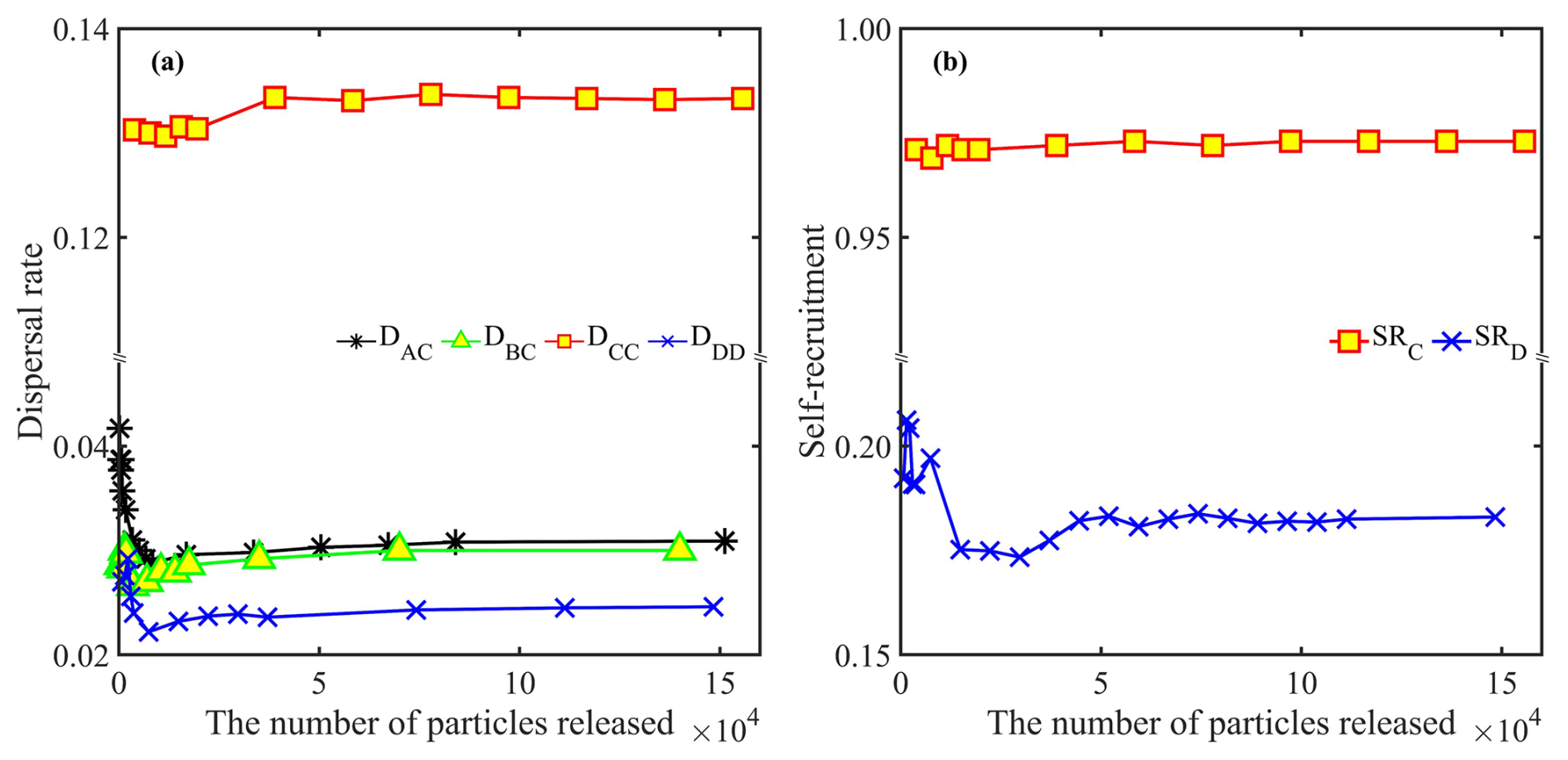
Figure 3 A sensitivity of results to the number of particles released. (a) In forward simulations, dispersal rates D_ij converge and become statistically stable when more than 40 000 particles are released. (b) In backward simulations, self-recruitment SR_i becomes stable above the same threshold.

4.2 Self-recruitment, local retention and relative local retention

In the forward-tracking simulations, the number of settled particles (F_ij) scaled directly with the number of particles released (N_i), whereas the dispersal rate (D_ij) remained independent of N_i (Table 1 and Fig. 3). Accordingly, both LR and RLR also showed negligible sensitivity to N_i. For example, LR at region C equalled D_CC≈0.13 and LR at region D equaled D_DD≈0.024. From Eq. (3), RLR was 0 at regions A and B, ∼0.76 at region C, and ∼0.99 at region D.

Table 1 Number of particles released from each region (N_i), the number settling in region (F_ij), the resulting dispersal rates (D_ij), and the corresponding local retention (LR_i), and relative local retention (RLR_i) from forward-tracking simulations. The four regions are the Detroit River Mouth (A), Western Shoreline (B), Midlake Reefs (C), and Bass Islands (D).

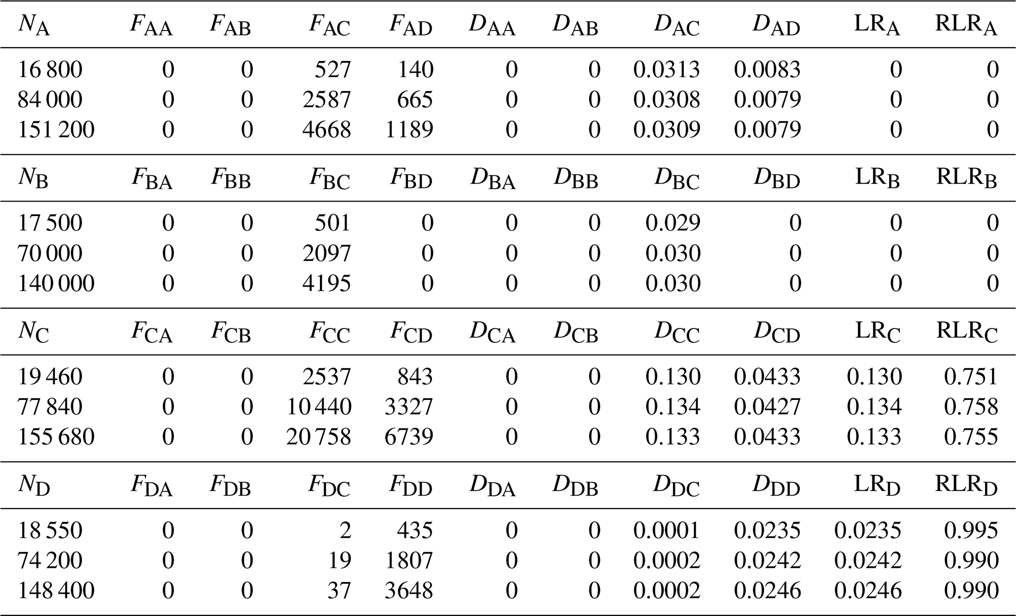
In contrast, SR estimates derived from forward-tracking varied markedly with N_i, reflecting the dependence of Eq. (3) on larval production at all source locations. Across the 81 forward-tracking configurations, SR at region C ranged from 0.22–0.95. For example, when releases were heavily weighted toward regions A and B (151 200 particles from A, 140 000 from B, 19 460 from C and 148 400 from D), ${\text{SR}}_c=\mathrm{2537}/(\mathrm{4668}+\mathrm{4195}+\mathrm{2537}+\mathrm{37})=\mathrm{0.22}$ whereas when releases were weighted toward region C (16 800 particles from A, 17 500 from B, 155 680 from C, and 18 550 from D), ${\text{SR}}_c=\mathrm{20}\mathrm{758}/(\mathrm{527}+\mathrm{501}+\mathrm{20}\mathrm{758}+\mathrm{2})=\mathrm{0.95}$. These outcomes demonstrate that SR from forward tracking is not uniquely defined unless the actual larval production $N_i^{\prime }$ is known and applied. Due to D_CC being much larger than D_AC, D_BC and D_DC, increasing N_C disproportionally increases the numerator of SR_C, causing SR to approach 1. Conversely, reducing N_C or increasing releases from other regions forces SR toward 0. Therefore, SR computed from forward-tracking can span the range [0,1] solely as a function of the assumed release numbers and cannot be interpreted biologically unless the actual number of larvae produced at each location is known and is released (i.e., $N_i=N_i^{\prime }$).

If all regions were assumed to release the same number of particles (a common but biologically unfounded modelling assumption), SR becomes only a function of D_ij. Under this scenario, ${\text{SR}}_{\mathrm{C}}=D_{\text{CC}}/D_{\text{AC}}+D_{\text{BC}}+D_{\text{CC}}+D_{\text{DC}}=\mathrm{0.68}$ and ${\text{SR}}_{\mathrm{D}}=D_{\text{DD}}/D_{\text{AD}}+D_{\text{BD}}+D_{\text{CD}}+D_{\text{DD}}=\mathrm{0.32}$. These values differ substantially from those obtained using backtracking.

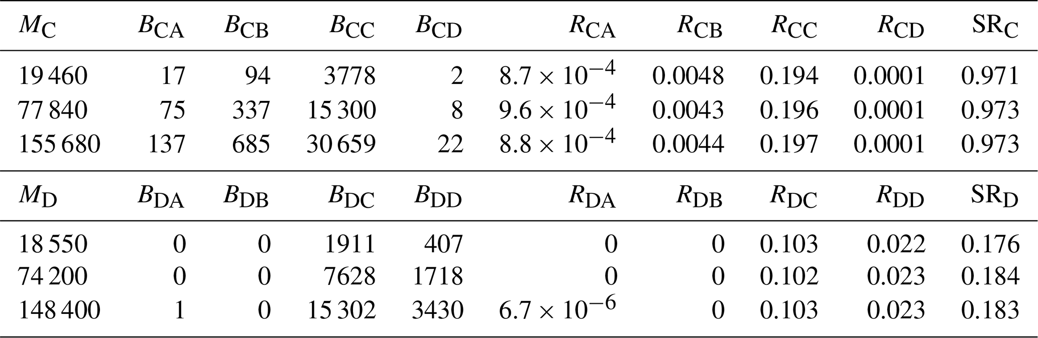
In the backtracking simulations, the number of particles traced to each location B_ij varied with the number released M_i, but the settlement rate R_ij and SR were consistent with M_i (Table 2 and Fig. 3). This stability shows that SR calculated from backtracking is independent of M_i, as indicated in Eq. (7).

Comparing backtracking and forward-tracking SR with equal release assumptions (i.e., N_i was the same for all sources) reveals the bias introduced by unknown or mis-specified larval production. For example, SR_C=0.97 and SR_D=0.18 from backtracking, but only 0.68 and 0.32, respectively, from forward tracking. The discrepancies arise because assuming equal N_i artificially inflates the contribution of weak sources (e.g., A and B) and suppresses the contribution of strong sources (i.e., C and D), thereby distorting the SR denominator.

Table 2 Number of particles released from each region (M_i) in the backtracking simulations, the number traced back to each region (B_ij), the resulting settlement rates (R_ij), and corresponding self-recruitment values (SR_i). The regions are the Detroit River Mouth (region A), Western Shoreline (B), Midlake Reefs (C), and Bass Islands (D).

4.3 Larval production

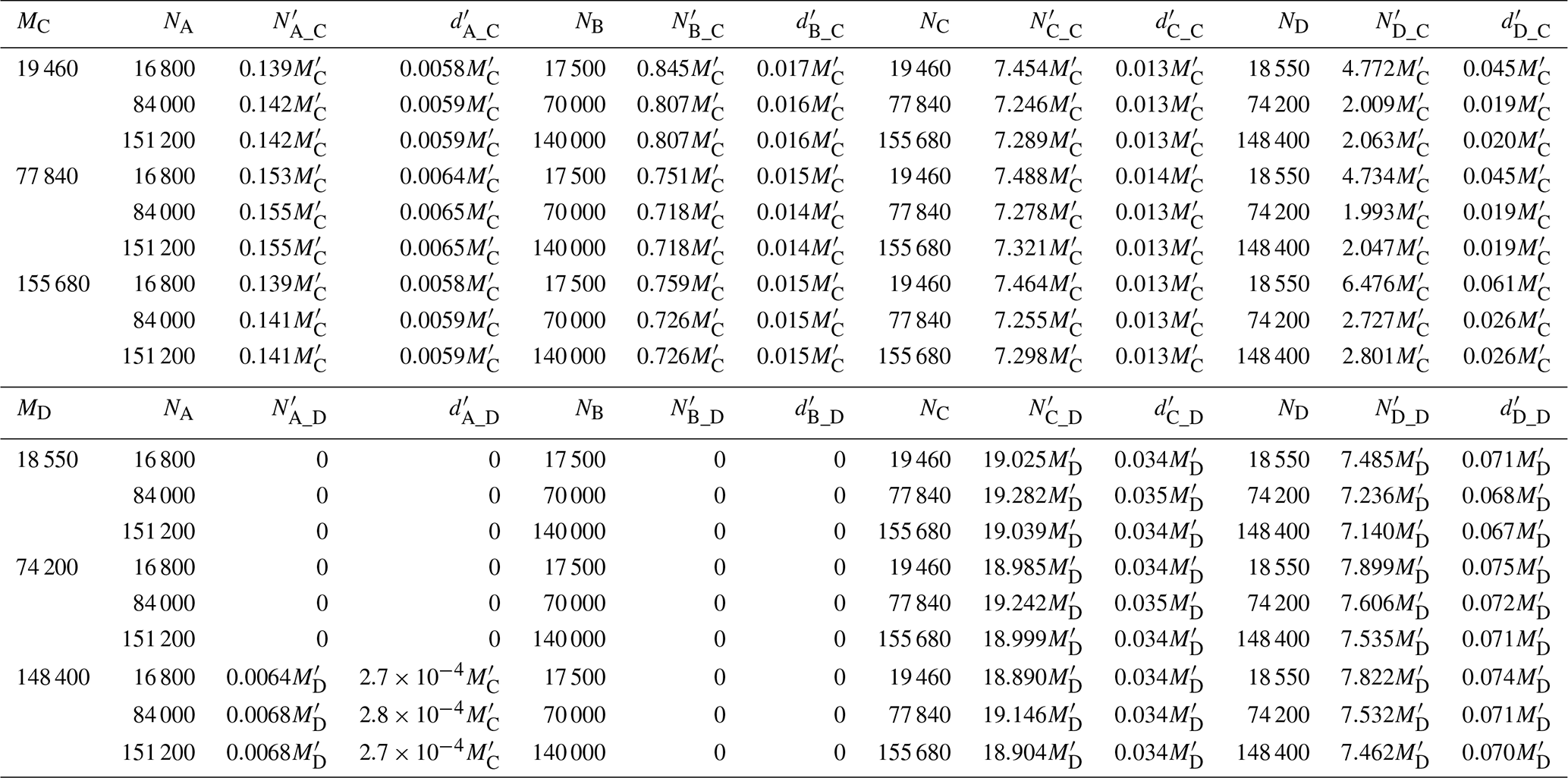
Using forward- and backward-tracking results, together with real recruits at regions C and D ($M_{\mathrm{C}}^{\prime }$ and $M_{\mathrm{D}}^{\prime }$), we estimated larval production at regions A, B, C and D based on Eqs. (10) and (16) (Table 3). When recruits at region C were used as the reference, estimated larval production at each region was largely insensitive to the number of particles released in the forward and backward tracking simulations, with the exception of region D, for which the dispersal rate from D to C (D_DC) was close to zero. When recruits at region D were used as the reference, estimated larval production at regions C and D also remained consistent, whereas estimates for regions A and B were zero due to the absence of recruitment to region D. These suggest that Eq. (10) provides a robust approach for estimating larval production.

The larval production density at region C computed from $M_{\mathrm{C}}^{\prime }$ ($d_{\mathrm{C}\mathit{\_}\mathrm{C}}^{\prime }$) was approximately $\mathrm{0.013}{M}_{\mathrm{C}}^{\prime }$, whereas that computed from $M_{\mathrm{D}}^{\prime }$ ($d_{\mathrm{C}\mathit{\_}\mathrm{D}}^{\prime }$) was approximately $\mathrm{0.034}{M}_{\mathrm{D}}^{\prime }$. Because $d_{\mathrm{C}\mathit{\_}\mathrm{C}}^{\prime }$ should equal $d_{\mathrm{C}\mathit{\_}\mathrm{D}}^{\prime }$, this yields that $\mathrm{0.013}{M}_{\mathrm{C}}^{\prime }=\mathrm{0.034}{M}_{\mathrm{D}}^{\prime }$, indicating that $M_{\mathrm{C}}^{\prime }\approx \mathrm{2.6}{M}_{\mathrm{D}}^{\prime }$. Similar, the larval production density at Region D computed from $M_{\mathrm{D}}^{\prime }$ ($d_{\mathrm{D}\mathit{\_}\mathrm{C}}^{\prime }$) was around $\mathrm{0.031}{M}_{\mathrm{C}}^{\prime }$, while that computed from $M_{\mathrm{D}}^{\prime }$ ($d_{\mathrm{D}\mathit{\_}\mathrm{D}}^{\prime }$) was around $\mathrm{0.071}{M}_{\mathrm{D}}^{\prime }$. Equating $d_{\mathrm{D}\mathit{\_}\mathrm{C}}^{\prime }$ and $d_{\mathrm{D}\mathit{\_}\mathrm{D}}^{\prime }$ yields $M_{\mathrm{C}}^{\prime }\approx \mathrm{2.3}{M}_{\mathrm{D}}^{\prime }$. The close agreement between these two independent estimates further supports the validity of Eq. (10) for estimating larval production. Notably, estimated larval production density followed a descending order from region D to region B to region C and finally to region A.

Table 3 Estimated larval production for each region ($N_{i\mathit{\_}\mathrm{C}}^{\prime }$ and $N_{i\mathit{\_}\mathrm{D}}^{\prime }$) based on the backtracking simulations initiated from regions C and D, respectively, together with the corresponding larval densities (number per AEM3D grid cell; $d_{i\mathit{\_}\mathrm{C}}^{\prime }$ and $d_{i\mathit{\_}\mathrm{D}}^{\prime }$). The regions are the Detroit River Mouth (A), Western Shoreline (B), Midlake Reefs (C), and Bass Islands (D).

5 Discussion

5.1 Estimates of self-recruitment

We have shown, using both theoretical arguments and numerical simulations, that self-recruitment (SR) cannot be unambiguously computed using forward Lagrangian particle tracking models. Forward-tracking studies have implemented a wide range of particle release strategies, including: (1) releasing a random number of larvae (Sato et al., 2023), (2) releasing an equal number of larvae (Dubois et al., 2016; Faillettaz et al., 2018), (3) scaling releases to habitat area (D'agostini et al., 2015), and (4) scaling releases to estimated larval production (Nolasco et al., 2022). Each strategy implicitly embeds an assumption about the spatial distribution of larval production, which is rarely known. As a result, SR estimates from forward tracking are sensitive to these assumptions.

For example, Sato et al. (2023) assumed equal larval production across 84 source locations in the Verde Island Passage and released 900 particles per location. After aggregating locations into three regions, they released 4500, 40 500 and 30 600 particles from Puerto Galera, the eastern region and the western region, respectively, giving $\text{SR}=\mathrm{17.9}/(\mathrm{17.9}+\mathrm{4.4}+\mathrm{71.9})=\mathrm{0.19}$ at Puerto Galera. However, if Puerto Galera was sub-divided into more spatial units, more particles would be released there, and the number of local settlers (17.9) would increase proportionally, altering SR. This example illustrates how SR can be influenced by arbitrary spatial partitioning.

Other studies apply different assumptions: D'agostini et al. (2015) proposed that larval production is proportional to habitat area; Saint-Amand et al. (2023) assumed a fixed larval density (500 larvae km⁻²); and Nolasco et al. (2022) scaled larval production to adult abundance and spawning intensity. In these examples, SR varied with the assumed production pattern and not solely with dispersal dynamics. Since it is often unknown whether larval production is uniform, area-proportional, or scales with adult biomass, forward-tracking estimates of SR inherit this uncertainty. Moreover, unmodelled or unknown source locations may contribute additional settlers, further biasing SR estimates.

In contrast, backward-in-time Lagrangian particle-tracking provides a more direct and robust framework for estimating SR. Backtracking releases particles from locations where juveniles are sampled and traces them backward to their origins. This method is widely applied to identify spawning or hatching sites (Christensen et al., 2007; Thygesen, 2011; Bauer et al., 2014; Gargano et al., 2022; Rowe et al., 2022; Chaput et al., 2023), but surprisingly few studies have used it to explicitly estimate SR. One exception is Torrado et al. (2021) who found high SR because most settlers originated from the same oceanographic region in which they settled.

A key advantage in backtracking is that the denominator of SR (the total number of settlers at location j) is simply the number of particles released from j and is allowed to be any convenient value (M_j). The key insight is that the resulting value of SR is independent of the absolute number of particles released (i.e., M_j in Eq. 7); our numerical results confirm this. Consequently, backtracking avoids the need to specify larval production at all source locations or to include every source explicitly. Rather, SR is estimated directly as the proportion of sampled recruits whose trajectories lead back to local origins, consistent with parentage-analysis studies (D'Aloia et al., 2013; Almany et al., 2017).

Although SR estimated from backtracking does not depend on M_j, it does depend on the physical environment. Variability in hydrodynamic conditions, spawning time and environmental forcing all impact SR. In our simulations, SR varied substantially between region C (0.97) and D (0.18), despite similar larval durations. Comparable variability has been documented in marine systems; for example, Paris et al. (2005) found that mutton snapper (Lutjanus analis) spawning aggregations in Cuba exported larvae regionally in patterns that produced distinct SR values. Even species spawning at the same location but at different times, may experience contrasting SR, as shifts in currents between lunar phases can alter dispersal pathways Paris et al. (2005).

Connectivity probability matrices (P_T), are widely used to summarise larval exchange among regions, and their diagonal elements are often interpreted as SR. However, because $P_{\mathrm{T},ij}=S_{\mathrm{T},ij}/{\sum }_i{S}_{\mathrm{T},ij}$, the denominator depends on larval production from all contributing source locations. Any change in assumed production therefore alters SR and all matrix elements. In contrast, normalising the transition matrix S_T by the total number of larvae released or surviving (${\sum }_j{S}_{\mathrm{T},ij}$) yields production-independent connectivity matrices whose diagonal elements reflect LR or RLR. This distinction reinforces our central result: forward-tracking estimates of SR inherently inherit assumptions about larval production, whereas SR estimated from backtracking does not.

5.2 Estimates of local retention and relative local retention

As indicated earlier, relative local retention (RLR) is typically more challenging to evaluate empirically than self-recruitment (SR) (Lett et al., 2015). SR can be estimated by sampling juveniles at a settlement site and identifying the proportion that originated locally using genetic parentage or assignment methods. In contrast, estimating RLR requires quantifying all larvae produced at a source location that ultimately survive and settle anywhere in the system. This includes individuals dispersed to distant or unsampled habitats, meaning that incomplete sampling directly biases the denominator of RLR.

Local retention (LR) is even more challenging to measure because it requires the total number of larvae produced at a location ($N_i^{\prime }$), including those lost to mortality or transported to unobserved locations. For example, Almany et al. (2017) assigned juveniles of Amphiprion percula and Chaetodon vagabundus to parents collected at eight sites Papua New Guinea, enabling estimation of the number of juveniles produced at each source location. However, it remained unknown whether larvae were transported exclusively among these eight sites, or whether additional sinks existed outside the sampling domain. Moreover, the total number produced at each site, including the fraction that died before settlement could not be determined.

These empirical limitations explain why forward-tracking studies commonly adopt simplified particle release strategies. Such approaches circumvent the need to estimate $N_i^{\prime }$, but they also mean that LR and RLR computed from forward models depend on assumptions about larval production.

5.3 Estimates of larval production and recruitment

Knowing the number of recruits at one settlement location ($M_i^{\prime }$) or the larval production at one source location ($N_i^{\prime }$) enables estimation of recruitment and production at all other locations from Eqs. (11) and (12). Equation (10) provides an approach to infer larval production at a source location ($N_i^{\prime }$) based on the number of recruits at a settlement site ($M_j^{\prime }$), together with the recruitment rate (R_ji) and the dispersal rate (D_ij). In principle, estimates of $N_i^{\prime }$ derived from different settlement locations should be consistent. For example, larval production at region C inferred using recruits from region C ($N_{\mathrm{C}\mathit{\_}\mathrm{C}}^{\prime }$) should equal that inferred using recruits form region D ($N_{\mathrm{C}\mathit{\_}\mathrm{D}}^{\prime }$). However, because the values of $M_{\mathrm{C}}^{\prime }$ and $M_{\mathrm{D}}^{\prime }$ are unavailable, this consistency cannot be directly verified. Nevertheless, it constrains their relative magnitudes, indicating that $M_{\mathrm{C}}^{\prime }\approx \mathrm{2.6}{M}_{\mathrm{D}}^{\prime }$. Similarly, larval production at region D inferred using recruits from regions C and D yields a comparable relationship, $M_{\mathrm{C}}^{\prime }\approx \mathrm{2.3}{M}_{\mathrm{D}}^{\prime }$. The close agreement between these two independent estimates provides partial support for the validity of Eq. (10) in estimating larval production.

Importantly, the framework also enables inference on relative larval production among locations. This information is of directly relevant to fisheries management, as it helps identify spawning and hatching grounds that contribute disproportionately to regional recruitment. By quantifying the relative contributions of different source locations, the approach provides a scientific basis for prioritizing habitat protection, restoration efforts, and spatially targeted management measures aimed at sustaining fish populations.

5.4 Implications and limitations of this research

Using forward and backward tracking models in combination provides a powerful framework for estimating not only SR and LR, but also larval production at each source location and the number of recruits at each settlement site. When used independently, backtracking models can only estimate SR (or imaginary SR) and settlement rates, while forward tracking models can only estimate LR (or relative LR) and dispersal rates. By integrating these two approaches, dispersal and settlement rates become linked, enabling the derivation of larval production at source locations and the number of recruits reaching all connected settlement sites once recruitment at any one location is known. This joint framework, therefore, supports the estimation of total larval production and total recruitment within a region, offering improved insight into population connectivity and direct utility for population assessment and fisheries management. Importantly, it enables quantification of the relative contributions of different spawning and hatching grounds to regional recruitment, helping to identify key source areas that disproportionately sustain population persistence. Such information is directly applicable to fisheries stock assessment, spatial management, and marine spatial planning, including the prioritization of critical habitats for protection or restoration.

Despite these advantages, several limitations remain in applying a backtracking model approach to evaluate SR. For example, diffusion cannot be reversed in time; backward diffusion is ill-posed and must be approximated using convergent schemes (Thygesen, 2011). Our simulations also used passive particles moving two dimensions and did not incorporate larval behaviours such as vertical migration or active swimming. Numerous studies have shown that incorporating larval behaviour in forward-tracking models can substantially alter dispersal outcomes (Berenshtein et al., 2018; Burgess et al., 2021; Faillettaz et al., 2018; James et al., 2019; Leis, 2020; Paris et al., 2005). Finally, our boundary condition, of removing particles when they intersect the model boundary, may introduce deviations between simulated and true dispersal pathways, which impacts SR estimates. Comparisons with empirical datasets are required to validate the backtracking-derived values of SR.

6 Conclusions

Our results demonstrate that self-recruitment (SR) fundamentally depends on the true larval production at all source locations capable of supplying recruits to the settlement site. Consequently, SR cannot be computed unambiguously in forward-tracking models unless all potential source locations and their respective larval production are known and used. This limitation is compounded by the different particle-release strategies employed in previous studies, which produce different SR estimates solely because they assume different production patterns. In contrast, empirical parentage analyses do not require quantifying larval production at every source location. SR is obtained directly as the proportion of sampled juveniles that originate locally. Backward-tracking models offer the same advantage: by releasing particles from a settlement site and tracing them backwards to their origins, SR is estimated as the fraction of locally sourced recruits. Our results confirm theoretically and numerically that SR computed from backtracking is independent of the number of particles released at the settlement locations, enabling the use of any release number and bypassing the need to identify all contributing source locations.

We further propose an approach to estimate larval production at each source location by combining information from forward- and backward-tracking models. When used separately, backtracking models provide only SR (or imaginary SR) and settlement rates, while forward-tracking models provide only LR (or relative LR) and dispersal rates. When used jointly they allow estimation of SR, LR, dispersal, settlement, larval production at source sites, and recruitment at all settlement sites, thereby offering a comprehensive framework for quantifying population connectivity.

Although demonstrated here for Lake Whitefish in Lake Erie, the theoretical and modelling framework apply broadly to both freshwater and marine species with pelagic larval phases. The ability to more accurately compute these metrics will improve understanding of population connectivity and support more informed management of spatially structured fish populations.

Appendix A

Table A1 Release regions, times and durations for forward and backward tracking simulations.

Table A2 The description of the notations in this research.