Quantifying charger-related uncertainty in electrical mobility analysis of aerosols with MPSS-UQ 1.0

Charging probability is the greatest source of uncertainty in electrical mobility-based measurements of aerosol size distributions, but its influence on the results is rarely quantified and reported. In bipolar charging, the charge distribution is almost universally modeled using the Wiedensohler approximation, although it has been shown to deviate significantly from the true charge distribution under many measurement conditions. The charge distribution depends, among other factors, on the mobilities of the charger ions, which are typically not precisely known. Ignoring this uncertainty can lead to biased size distribution estimates and severe underestimation of their uncertainty. In this work, we quantify the uncertainty that imprecisely known charger ion mobilities introduce into the charged particle fractions, and then propagate this uncertainty into the estimates of the particle size distributions using a modular Bayesian approach, in which the ion mobilities are treated as nuisance parameters and marginalized over their plausible range. The inversion method, which is available as the open-source Python package MPSS-UQ, is implemented with particular emphasis on computational efficiency and tested with both synthetic and real mobility particle size spectrometer data. For a month-long field dataset, marginalizing over the uncertain ion mobilities widened the posterior credible intervals of the estimated size distributions on average by a factor of 2.4, with factors up to 10 in some size classes, compared to conditioning on fixed mobility values. The wider intervals provide a more realistic assessment of uncertainties in the inferred size distributions, and quantifying the structure of this uncertainty helps identify where improvements in the characterization of charger ion properties or in the measurement setup would be most effective.

1 Introduction

Electrical mobility analysis, carried out with a mobility particle size spectrometer (MPSS) (Knutson and Whitby, 1975; Wang and Flagan, 1990), is the primary technique for near-real-time in-situ measurement of the particle size distribution (PSD) of submicron aerosols (Flagan, 2008) and is commonly used for long-term atmospheric observations. The technique requires that the particles are brought to a known and stationary charge distribution, typically with a bipolar charger. The charged particles are then separated by their electrical mobility and, hence, size by a differential mobility analyzer (DMA) and counted with a condensation particle counter (CPC) to yield a measured electrical mobility distribution. These instruments are typically operated either in a stepwise mode, known as a Differential Mobility Particle Sizer (DMPS), or in a continuous scanning mode, known as a Scanning Mobility Particle Sizer (SMPS). The remaining problem is then to infer the PSD of the aerosol at the inlet of the charger based on the measured counts.

Due to the importance of assessing the contribution of submicron aerosols to, for example, adverse health effects (Shiraiwa et al., 2017; Manisalidis et al., 2020) and climate change (Bellouin et al., 2020; Kahn et al., 2023), it is imperative that the limitations and uncertainties of the MPSS are well understood. Inter-comparison and calibration studies (Wiedensohler et al., 2012, 2017) show that in carefully controlled environments MPSS measurements over the range of 20 to 200 nm are reproducible to within 10 % relative deviations in the estimated PSD. A set of 12 commercial and custom-made inversion routines, given an identical set of measurements, was also shown to agree to within ±5 %. This implies that the DMA and CPC can be tuned to enable high accuracy of measurement, but similar conclusions about the charger cannot be made for two reasons: (i) the charging process depends on the mobilities of the charging ions, which in turn depend on environmental factors, such as the composition of the carrier gas and possible trace constituents found in it, that are not always controllable and usually at least partly unknown (Mäkelä et al., 1996; Steiner and Reischl, 2012; Schmidt-Ott et al., 2024), and (ii) all of the tested methods (and more generally most of the MPSS inversion methods (ISO 15900:2009(E), 2009; TSI, 2016; Flagan, 2008)) use the same, readily evaluated Wiedensohler approximation (Wiedensohler, 1988) for charging probability, and do not consider charger-related uncertainty. Inter-comparison measurements made in the same environment assuming the same charging probability cannot show relative deviations due to the charging fraction. In addition to the uncertainty from environmental random effects, most models for approximating the charge distribution are based on at least some idealized assumptions such as spherical particles and monodisperse ions with a single mobility and mass value. These reasons make the charging probability the largest source of uncertainty in MPSS measurements (López-Yglesias and Flagan, 2013).

The sensitivity of the charge distribution to uncertainties in ion properties and environmental conditions can be quantified numerically with charging models. The ion mobility has been shown to vary by up to 40 %–60 % due to differences in the composition and purity of the carrier gas (Steiner and Reischl, 2012; Schmidt-Ott et al., 2024). These realistic variations in ion mobilities were shown by Tigges et al. (2015) to lead to about ±25 % typical (and up to 50 % in extreme cases) differences in the predicted charge fractions compared to the Wiedensohler approximation. Results by Steiner and Reischl (2012), on the other hand, showed that the charging probability varies only slightly (up to 8 % for particles <10 nm but less than 1 % for particles >70 nm) despite the large variation in ion mobility. An explanatory factor for these differences may be that the charge fractions in Steiner and Reischl (2012) were calculated using the Fuchs model (Fuchs, 1963), whereas in Tigges et al. (2015) they were calculated with the Fuchs model including corrections by Hoppel and Frick (1986).

The potentially large uncertainties in the charging probability lead naturally to the question: how much does the error induced by using an incorrect charge distribution influence the estimated size distribution? This also can be assessed numerically, by inverting simulated MPSS measurements with the correct and approximate charging probabilities, as in Leppä et al. (2017) who found that using an incorrect charging probability can result in up to a factor of 5 difference between the true and estimated particle numbers of the nucleation mode, and up to 80 % for larger particles. Such large errors emphasize that to properly assess the reliability of MPSS measurements, uncertainty estimates based on systematic uncertainty quantification that accounts for the charging probability should always accompany the size distribution estimates. However, although the typical sources of uncertainties in MPSS are well understood (Kangasluoma and Kontkanen, 2017; Wiedensohler et al., 2017; Coquelin et al., 2018; Kangasluoma et al., 2020; CEN/TS, 2020), the practice of providing any uncertainty estimates is rare in studies reporting MPSS measurements (see, for example, Dal Maso et al., 2005; Väänänen et al., 2013; Portin et al., 2014; Deng et al., 2022; Sorooshian et al., 2023; Zhang et al., 2026) and further the MPSS inversion methods themselves are not usually developed with uncertainty quantification in mind (Świrniak and Mroczka, 2022; Sipkens et al., 2023; Vasilatou et al., 2025).

In this work, we develop a method for MPSS inversion based on the Bayesian approach (Kaipio and Somersalo, 2005; Gelman et al., 2013), where both the measurements and the unknown quantities, such as the PSD and the charging probability, are treated in a probabilistic manner. In this framework, a prior model for the unknown parameters is combined with the likelihood of the measurements to produce a posterior probability distribution, which is then used to compute estimates of the unknown parameters and their uncertainties. Previous studies have addressed aspects of uncertainty or model complexity in MPSS data analysis, but in ways that differ substantially from our approach. Ramachandran and Kandlikar (1996) and Voutilainen et al. (2001) formulated the inversion problem in the Bayesian framework, but they did not explicitly account for uncertainties in charging probability. Voutilainen and Kaipio (2001) extended the method to a state-space framework and applied Kalman filtering and smoothing to improve temporal resolution for non-stationary size distributions. More recently, Coquelin et al. (2018) proposed a Monte Carlo-based framework for uncertainty propagation in SMPS measurements, modeling various sources of experimental and physical uncertainty, including charging effects, through stochastic parameter sampling. However, their approach is not Bayesian and treats charging probability uncertainty only in an approximate manner, using a Gaussian fit to predictions from the Fuchs theory. In contrast, our work is based on a fully Bayesian uncertainty quantification framework that systematically incorporates charging probability uncertainty into the inversion process. Specifically, we account for the uncertainty in the charging probability by modelling the charger ion mobilities as nuisance parameters to be marginalized. To enable treatment of particle concentrations that may span multiple orders of magnitude, we parametrize the size distribution on a log ₁₀-scale. In addition, we provide a Python-based code package MPSS-UQ (Niskanen, 2026), which has been used to compute all the results in this paper and can be readily used for uncertainty quantification (UQ) in MPSS measurements.

The rest of the paper is organised as follows: The bipolar charge distribution and uncertainties related to it are discussed in Sect. 2. In Sect. 3, we then define the estimation problem in the framework of Bayesian inference, and in Sect. 4 show examples of the calculated uncertainties with synthetic and real data. Discussion and conclusions are given in Sects. 5 and 6, respectively.

2 A model for the MPSS and charging probability

2.1 The forward model

Let us first briefly recall the forward model of a typical MPSS. The forward model is a deterministic mapping from the size distribution, or its discretization, to the expected, noiseless, measurements. The actual measurements will differ from the expectation due to stochastic uncertainties, which we will model later in Sect. 3.2. Assume that we have selected I channels to measure, where each channel i is associated with a nominal (i.e., assumed to be singly-charged) particle mobility diameter, which can also be stated as a target electrical mobility Z_i that we want to classify, which also determines a set DMA voltage. We will express particle size on a log ₁₀-scale, which is the typical convention, and hence define the size distribution function as $n\left(d\right)=\frac{\mathrm{d}N}{\mathrm{d}{\log }_{\mathrm{10}}d}$ [cm⁻³ per decade], where N is the cumulative size distribution and d is the particle mobility diameter. For a continuous size distribution, the expected particle counts ${\stackrel{\mathrm{̃}}{y}}_i$ measured by the CPC in channel i are:

$$\begin{array}{}\text{(1)}& \begin{array}{rl}{\stackrel{\mathrm{̃}}{y}}_i=\mathcal{V}\underset{{\log }_{\mathrm{10}}\left(d_{\min }\right)}{\overset{{\log }_{\mathrm{10}}\left(d_{\max }\right)}{\int }}& \sum _{p}T\left(Z(d,p),Z_i\right)f_p\left(d\right)\\ & \mathit{\eta }\left(d\right)n\left(d\right)\mathrm{d}{\log }_{\mathrm{10}}d,\end{array}\end{array}$$

where 𝒱 is the sampled volume, d_min and d_max denote the smallest and largest considered mobility diameters, respectively, $T\left(Z(d,p),Z_i\right)$ is the DMA transfer function for channel i where Z(d,p) denotes the electrical mobility of a particle with diameter d and charge p. The transmission and detection efficiencies, including sampling lines and the DMA penetration efficiency as well as the CPC counting efficiency, are represented by η(d), and f_p(d) is the charging probability, the probability that a particle of size d carries p elementary charges.

To derive a discrete form of Eq. (1), we divide the size range [log ₁₀(d_min),log ₁₀(d_max)] into M bins, with the jth bin as ${\mathrm{\Delta }}_j=\left[{\log }_{\mathrm{10}}\right(d_j^{\mathrm{left}}),{\log }_{\mathrm{10}}(d_j^{\mathrm{right}}\left)\right]$, denoting its midpoint (geometric mean of the edges) by d_j and width by $\left|\mathrm{\Delta }{\log }_{\mathrm{10}}{d}_j\right|$. Further, for simplicity let us assume that in each bin the number concentration n(d), the penetration and detection efficiency η(d), and charging probability f_p(d) vary smoothly enough as function of d so that we can approximate them as constant, taking their midpoint values n(d_j),η(d_j), and f_p(d_j), which we will denote by n_j,η_j, and f_p,j. That leaves only the transfer function to be integrated, which we carry out with the trapezoidal rule. Taking all constant terms outside the integral, the discretized version reads

$$\begin{array}{}\text{(2)}& {\stackrel{\mathrm{̃}}{y}}_i\approx \mathcal{V}\sum _{j=\mathrm{1}}^M\left(\sum _p{f}_{p,j}\underset{{\mathrm{\Delta }}_j}{\int }T\left(Z(d,p),Z_i\right)\mathrm{d}{\log }_{\mathrm{10}}d\right){\mathit{\eta }}_j{n}_j.\end{array}$$

Now denote the integral of the transfer function, normalized by the bin width $\left|\mathrm{\Delta }{\log }_{\mathrm{10}}{d}_j\right|$, by

$$\begin{array}{}\text{(3)}& {\stackrel{\mathrm{̃}}{T}}_{ij,p}={\displaystyle \frac{\mathrm{1}}{\left|\mathrm{\Delta }{\log }_{\mathrm{10}}{d}_j\right|}}\underset{{\mathrm{\Delta }}_j}{\int }T\left(Z(d,p),Z_i\right)\mathrm{d}{\log }_{\mathrm{10}}d,\end{array}$$

define the MPSS kernel, or instrument matrix, for output channel i and size bin j

$$\begin{array}{}\text{(4)}& A_{ij}=\mathcal{V}\sum _p{f}_{p,j}{\stackrel{\mathrm{̃}}{T}}_{ij,p}{\mathit{\eta }}_j,\end{array}$$

and represent the size distribution using the total particle concentration in a bin $N_j:=n_j\left|\mathrm{\Delta }{\log }_{\mathrm{10}}{d}_j\right|$. The forward model can then be written in matrix form as

$$\begin{array}{}\text{(5)}& \stackrel{\mathrm{̃}}{\mathit{y}}=h\left(\mathbf{N}\right)=\mathbf{AN},\end{array}$$

where $\stackrel{\mathrm{̃}}{\mathit{y}}=({\stackrel{\mathrm{̃}}{y}}_{\mathrm{1}},\mathrm{\dots },{\stackrel{\mathrm{̃}}{y}}_I{)}^{\mathsf{T}}$, $\mathbf{N}=(N_{\mathrm{1}},\mathrm{\dots },N_M{)}^{\mathsf{T}}$, and h(⋅) denotes the forward operator that maps the discretized size distribution to the expected CPC counts. The exact forms of the DMA transfer function, the sampling losses, and the counting efficiencies implemented in MPSS-UQ are given in Appendix A.

2.2 Uncertainty in the bipolar charge fraction

Since the MPSS forward model (Eq. 1) depends explicitly on the particle charge distribution, any deviation from the expected distribution can significantly affect the PSD estimates. Let us now investigate the magnitude of the uncertainty in the charge distribution.

A common way to achieve a (in principle known) steady state charge distribution is by bipolar diffusion charging, also known as neutralization. Compared to unipolar charging, bipolar charging has a rather low charging efficiency, especially for small (<10 nm) particles (Reischl et al., 1996), but the upside is that the charge distribution produced is not as highly dependent on the charging conditions and thus the reproducibility of the charge distribution is better. In bipolar charging, the aerosol is exposed to a high concentration of positive and negative ions which transfer charge to the particles in ion-particle collisions. After a sufficient amount of time the process results in a stationary charge distribution with both positively and negatively charged particles, whose net charge is close to zero but typically slightly negative due to the higher attachment probability of negative vs. positive ions. For sufficient conditions to reach stationarity see for example Adachi et al. (1989); de La Verpilliere et al. (2015); Ibarra et al. (2020). Also note that the charge distribution keeps evolving in the tubing downstream of the charger (Nishida et al., 2025). In this paper, we assume that the concentration of the ions is high enough and the residence time in the charger is long enough to achieve a stationary charge distribution, but we do not model its evolution past the charger.

To model the bipolar charge distribution numerically we use the Fuchs theory (Fuchs, 1963) as extended and corrected by Hoppel and Frick (1986) and later by López-Yglesias and Flagan (2013). We will henceforth refer to this model as the LYF model. The model is based on the limiting sphere approach, where the space around the particles is divided into two zones, an outer diffusional zone and an inner low collisionality zone, which are separated by the limiting sphere. Inside the limiting sphere, particle motion is idealized to be purely ballistic which necessitates the use of correction terms such as three-body trapping, whereas in the diffusional zone the motion follows the principles of continuum mechanics. The LYF model has been shown to be in good agreement with experimental data on particle-ion collision rates in atmospheric conditions (Pfeifer et al., 2023), but note that there are other approaches (Gatti and Kortshagen, 2008; Gopalakrishnan and Hogan, 2012; Gopalakrishnan et al., 2013; Li et al., 2020) that we could use as well. In the following, we will discuss some input parameters and some computational aspects of our implementation of the LYF model in MPSS-UQ. For a complete theoretical description of the model we refer to López-Yglesias and Flagan (2013) and the references therein.

The LYF model characterizes ion–particle collision dynamics through the ion flux coefficient ${\mathit{\beta }}_{q,\pm }\left(d\right)$ which represents the rate at which positive or negative ions attach to a particle of diameter d with q elementary charges. For simplicity, we denote the model by ℱ_LYF and express this relationship symbolically as

$$\begin{array}{}\text{(6)}& {\mathit{\beta }}_{q,\pm }\left(d\right)={\mathcal{F}}_{\mathrm{LYF}}(d,Z^{\pm },m^{\pm },T,\mathit{\mu },M_{\mathrm{gas}},P),\end{array}$$

where d is the particle diameter, Z^± and m^± are the ion mobility and mass, and T, μ, M_gas, and P are the temperature, viscosity, mass, and pressure of the carrier gas, respectively. To keep notation light, in the following we suppress the explicit dependence of ${\mathit{\beta }}_{q,\pm }$ and f_p on particle diameter d. Note that the ion mobilities themselves depend on the chemical composition of the carrier gas (Steiner and Reischl, 2012). The carrier gas hence influences the charge fraction both directly via collision dynamics and indirectly via ion mobility. In the sensitivity analysis here, we consider only the effect of varying the ion mobility and compute the corresponding ion masses m^± deterministically as shown below, while setting the gas properties to nominal values of T=298 K, $\mathit{\mu }=\mathrm{18.27}\times {\mathrm{10}}^{-\mathrm{6}}$ Pa s, M_gas=28.97 amu, and P=101 325 Pa.

The fraction f_p of particles carrying p charges can be calculated from the flux coefficients as (Gopalakrishnan et al., 2013; Lòpez-Yglesias and Flagan, 2013)

$$\begin{array}{}\text{(7)}& f_p={\displaystyle \frac{\mathrm{1}}{\mathrm{\Omega }}}\left\{\begin{array}{ll}{\prod }_{q=\mathrm{1}}^p{\displaystyle \frac{{\mathit{\beta }}_{q-\mathrm{1},+}}{{\mathit{\beta }}_{q,-}}}{\displaystyle \frac{n_{+}}{n_{-}}}& ;p\ge +\mathrm{1}\\ \mathrm{1}& ;p=\mathrm{0}\\ {\prod }_{q=p}^{-\mathrm{1}}{\displaystyle \frac{{\mathit{\beta }}_{q+\mathrm{1},-}}{{\mathit{\beta }}_{q,+}}}{\displaystyle \frac{n_{-}}{n_{+}}}& ;p\le -\mathrm{1}\end{array}\right.,\end{array}$$

where n_± denotes the number concentration of positive or negative ions (not to be confused with the particle size distribution n(d)). The normalization constant Ω is given by

$$\begin{array}{}\text{(8)}& \begin{array}{rl}\mathrm{\Omega }=& \sum _{p=-\mathrm{\infty }}^{-\mathrm{1}}\left\{\prod _{q=p}^{-\mathrm{1}}{\displaystyle \frac{{\mathit{\beta }}_{q+\mathrm{1},-}}{{\mathit{\beta }}_{q,+}}}{\displaystyle \frac{n_{-}}{n_{+}}}\right\}+\mathrm{1}\\ & +\sum _{p=\mathrm{1}}^{\mathrm{\infty }}\left\{\prod _{q=\mathrm{1}}^p{\displaystyle \frac{{\mathit{\beta }}_{q-\mathrm{1},+}}{{\mathit{\beta }}_{q,-}}}{\displaystyle \frac{n_{+}}{n_{-}}}\right\}.\end{array}\end{array}$$

Various measurements of the ion mobilities have been carried out over time, using several types of radioactive and X-ray sources. An extensive list of these has been compiled by Tigges et al. (2015), and we summarize the reported mobility values in Fig. 1a. The measured ion mobilities vary over a rather large range, between $Z^{+}\in [\mathrm{1.1},\mathrm{1.65}]$ ${\mathrm{cm}}^{\mathrm{2}}{\mathrm{V}}^{-\mathrm{1}}{\mathrm{s}}^{-\mathrm{1}}$ and $Z^{-}\in [\mathrm{1.15},\mathrm{2.10}]$ ${\mathrm{cm}}^{\mathrm{2}}{\mathrm{V}}^{-\mathrm{1}}{\mathrm{s}}^{-\mathrm{1}}$ with the condition $Z^{-}\ge Z^{+}$. Further, the ion source does not seem to correlate with the mobility values. We therefore define as the plausible range of ion mobilities in an MPSS measurement to consider a trapezoid-like shape around the measured values, denoted by the shaded area in Fig. 1a. Note that the mobilities $Z^{+}=\mathrm{1.35}$ ${\mathrm{cm}}^{\mathrm{2}}{\mathrm{V}}^{-\mathrm{1}}{\mathrm{s}}^{-\mathrm{1}}$ and $Z^{-}=\mathrm{1.60}$ ${\mathrm{cm}}^{\mathrm{2}}{\mathrm{V}}^{-\mathrm{1}}{\mathrm{s}}^{-\mathrm{1}}$ used in the Wiedensohler approximation are approximately in the middle of this trapezoid.

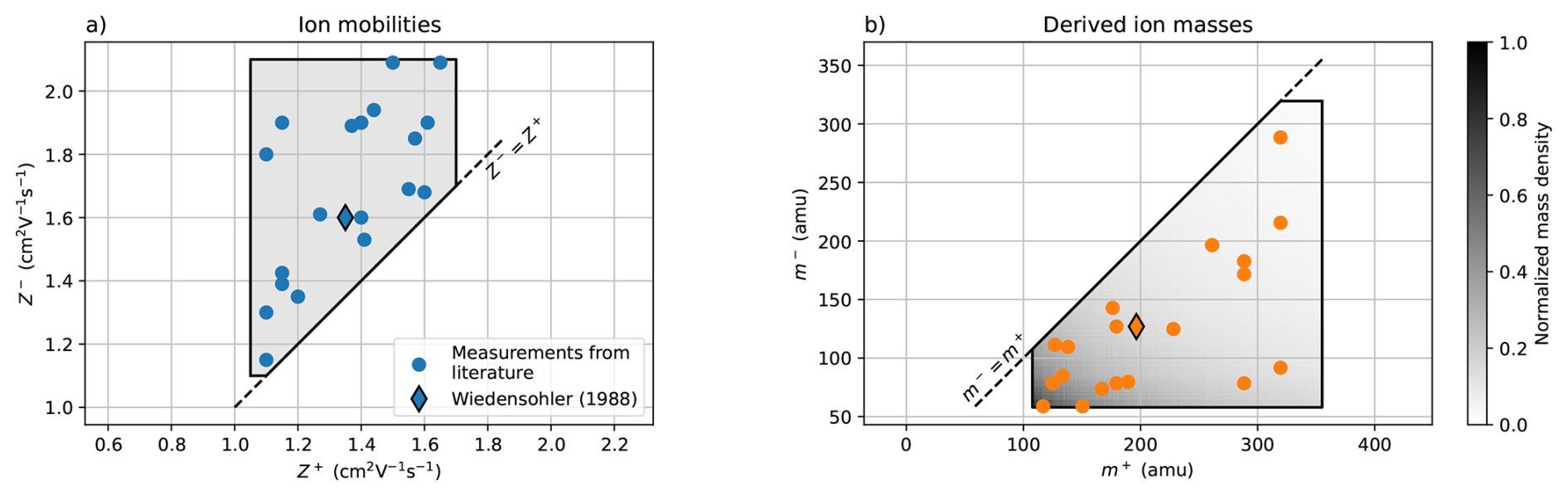
Figure 1 (a) Measurements of ion mobilities from the literature (compiled by Tigges et al., 2015), with the parameters used in Wiedensohler (1988) marked separately. The shaded area denotes the range of ion mobilities we consider in this work. (b) Ion masses derived from the measured mobilities using Eq. (9). The shading (normalized mass density) shows how the uniform density of mobilities results in a non-uniform density of mass concentrated towards the bottom left due to the nonlinear transformation.

There are considerably fewer studies on the ion masses, and the relationship between the ion mobility and mass also depends on the species of the ion. The ion mass could in principle be inferred from the Stokes-Millikan relation (Davies, 1945), and there are also more detailed scattering-based mobility models applicable to ions in diatomic gases (Larriba and Hogan, 2013), but in this work we use the empirical relationship by Mäkelä et al. (1996) which is a fit to the experimental data of Kilpatrick (1971) obtained for a variety of gas-phase ion species:

$$\begin{array}{}\text{(9)}& Z=\exp \left[-\mathrm{0.0347}\left(\ln \right(m_{\mathrm{i}}){)}^{\mathrm{2}}-\mathrm{0.0376}\ln (m_{\mathrm{i}})+\mathrm{1.4662}\right],\end{array}$$

where m_i is the ion mass in amu, and Z is the ion mobility in ${\mathrm{cm}}^{\mathrm{2}}{\mathrm{V}}^{-\mathrm{1}}{\mathrm{s}}^{-\mathrm{1}}$. Using this relationship, the measured ion mobilities map to masses as shown in Fig. 1b. The nonlinear mapping pushes the derived masses towards the corner with smaller values. This effect is also apparent in the derived probability density of the mass, obtained by assuming a uniform probability for the ion mobility over the trapezoid.

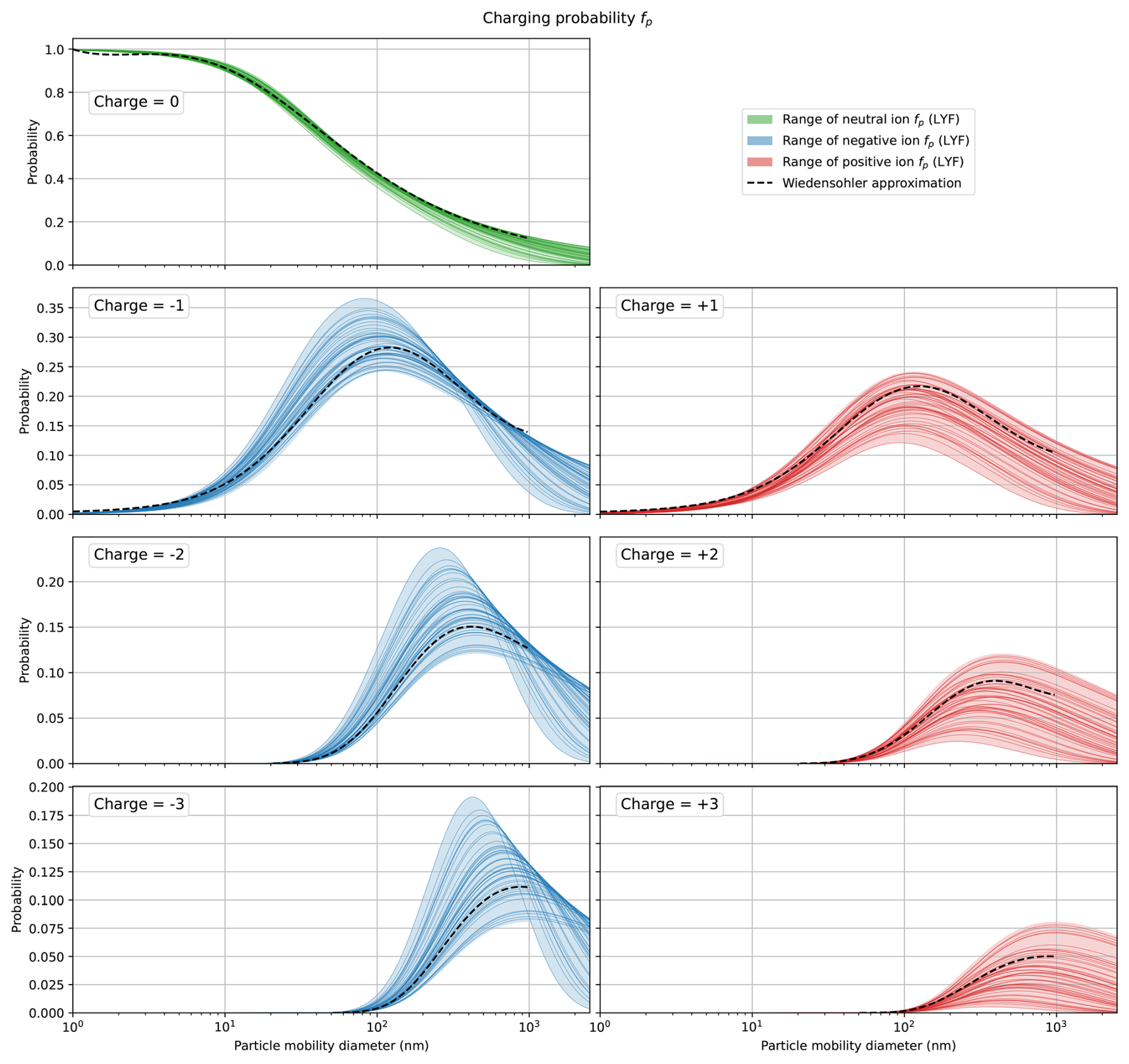
Figure 2 Charging probabilities predicted by the Lopez-Yglesias-Flagan (LYF) model for particle charges $\mathrm{0},\pm \mathrm{1},\pm \mathrm{2},\pm \mathrm{3}$, when the ion mobilities are varied according to Fig. 1a. The shaded areas indicate the maximum range of the model predictions, and the individual colored lines are LYF model predictions for random draws of the positive and negative ion mobilities, shown for illustrative purposes. The Wiedensohler approximation is shown for comparison.

To demonstrate the range of plausible charging probabilities, we can now take the area of the charger ion mobilities (and, derivatively, masses) considered in Fig. 1 and put it through the LYF model. Specifically, we divide the ion mobility trapezoid into a grid of 1400 uniformly spaced points of ion mobility pairs $(Z_k^{+},Z_k^{-})$, calculate the charging probability for every pair, and then pool the results together. The ranges of the resulting charging probabilities for charges $p\in [-\mathrm{3},\mathrm{3}]$ are shown in Fig. 2, along with the charging probability given by the Wiedensohler approximation. This charging probability range is the starting point for propagating the charging uncertainty into the size distribution estimates which is treated in the next section.

Table 1 shows the mean and 99th percentile relative deviations between the LYF model output range and the Wiedensohler approximation, for the charges $p\in [-\mathrm{3},\mathrm{3}]$. We calculate the relative difference as

$$\begin{array}{}\text{(10)}& {\displaystyle \frac{|f_{p,\mathrm{W}}-f_{p,\mathrm{LYF}}|}{\left|f_{p,\mathrm{W}}\right|+\mathit{ϵ}}},\mathrm{with}\mathit{ϵ}={\mathrm{10}}^{-\mathrm{9}},\end{array}$$

where the subscripts refer to the said models. The small ϵ is added to the denominator to stabilize the computation of the relative error for very small values of f_p where tiny absolute differences could show as large relative differences, and $\mathit{ϵ}={\mathrm{10}}^{-\mathrm{9}}$ is chosen empirically based on sensitivity tests that show that charging probabilities smaller than 10⁻⁸ have a negligible influence on the inversion. Only the size ranges where the Wiedensohler approximation is valid are used in the calculation of the relative difference.

Table 1 The mean and 99th percentile relative differences between the Wiedensohler approximation and the considered LYF model outputs for the most probable charge states.

Evaluating the LYF model can be computationally heavy in practice. For example, our Python implementation takes approximately 3 min to compute a single prediction of the charging probabilities (computed for 60 size bins and considering 51 charge states between $p=-\mathrm{25},\mathrm{\dots },\mathrm{25}$), which would make it unfeasible to carry out the uncertainty calculations where the model has to be evaluated at least a few tens of times per measurement. To make computing the LYF charging probability feasible for practical applications, we approximate the model by cubic interpolation based on precomputed values. The precomputations are carried out for 100 pairs of positive and negative ion mobilities and 40 particle diameters between the range 1 to 2500 nm and for each input value we store both the flux coefficients ${\mathit{\beta }}_{q,\pm }(d;Z^{+},Z^{-})$ (to enable calculation of the charging probability as in Eq. (7) with varying ion ratios) and the charging probability $f_p(d;Z^{+},Z^{-})$ assuming the ion ratio is unity (for maximum evaluation speed in that case). Using the interpolator is over 10⁵ times faster than evaluating the LYF model directly, but obviously some interpolation error is introduced. In a test that considered 15 randomly chosen ion pairs, charges between $-\mathrm{10},\mathrm{\dots },\mathrm{10}$, and 60 logarithmically spaced diameters between 1 and 2500 nm, the mean relative difference between the directly evaluated and the interpolated outputs, calculated as in Eq. (10), was found to be 0.052 % and the 99th percentile relative error was 0.95 %.

3 Bayesian MPSS inversion

Let us now consider the inversion problem: estimating the PSD based on the MPSS measurements. As mentioned, we adopt the Bayesian framework for inverse problems (Kaipio and Somersalo, 2005; Gelman et al., 2013), which allows us to include multiple sources of uncertainty, such as measurement noise and modeling errors, into the estimation process. Moreover, the resulting uncertainty estimates have an intuitive and natural interpretation: Bayesian credible intervals, unlike the frequentist confidence intervals, are directly statements on the probabilities of the unknown, conditional on the model and prior assumptions. For example, a 95 % credible interval means that, given the data and the model, there is a 95 % probability that the true value lies within the interval. In this work, we define the credible interval as the contiguous highest density interval, where every point inside has a higher posterior density than any point outside. The highest density interval is also the shortest possible credible interval.

The Bayesian solution is the posterior distribution, which expresses the probability of the unknown parameters conditioned on the measured data. Let x denote the unknown parameters of interest. In the simplest case in MPSS inversion, x=N, where N represents a discretized form of the PSD, but the formulation allows for inclusion of additional unknowns if needed as will be shown later in Sect. 3.4. The unknowns are first given a prior probability density, π(x), which models statistically the information available about the parameters before the measurements are taken into account. It should be broad enough to contain all plausible (or expected) values and can also encode domain knowledge such as smoothness of the PSD. Measurement data y are then incorporated through the likelihood function π(y|x), which quantifies how well different parameter values explain the measurements, accounting for noise and model discrepancies. In the MPSS context, the likelihood is derived from the observation model introduced in Sect. 2.1. The likelihood and prior combined form the posterior probability density:

$$\begin{array}{}\text{(11)}& \mathit{\pi }\left(\mathit{x}\right|\mathit{y})={\displaystyle \frac{\mathit{\pi }\left(\mathit{y}\right|\mathit{x}\left)\mathit{\pi }\right(\mathit{x})}{\mathit{\pi }\left(\mathit{y}\right)}}\propto \mathit{\pi }(\mathit{y}\left|\mathit{x}\right)\mathit{\pi }\left(\mathit{x}\right),\end{array}$$

where π(y) is the marginal likelihood, which acts as a normalization constant and can usually be ignored. The posterior then represents the prior distribution updated by the likelihood, assigning higher probability to regions of the parameter space that are consistent with both prior beliefs and observations.

3.1 Formulating the prior

We first consider the parametrization of the PSD, which falls in the category of prior assumptions even though it does not come in the form of a probability density. Two requirements guide the choice of parametrization: it should treat all orders of magnitude of the number concentration equally, so that no particular scale is favoured a priori, and it should enforce positivity of the number concentration. To see why the first point matters, consider a prior probability density for N of the form $\mathbf{N}\sim \mathcal{U}\left(\right[\mathrm{0},{\mathrm{10}}^{\mathrm{7}}\left]\right)$, where 𝒰 denotes the uniform distribution, i.e., the probability density is constant over the interval [0,10⁷], which at first sight treats all values equally. However, this implicitly places a strong prior towards the highest concentrations: the probability that N is in the range [10⁶,10⁷] is 0.9, while for example the probability of N being in [10²,10³] is only $\mathrm{9}\times {\mathrm{10}}^{-\mathrm{5}}$. Ideally, we would like to be “prior ignorant” about the number concentration. The second point is obvious; number concentrations cannot be negative. There are many ways to enforce the non-negativity, but a natural choice is to build it into the parametrization itself.

The logarithmic transform satisfies both requirements and therefore we choose to represent the size distribution on a log ₁₀-scale, so that x:=log ₁₀(N). In addition to enforcing positivity, this has the benefit of reflecting uncertainty about the scale rather than the absolute concentration. If we place on x a uniform prior $\mathit{x}\sim \mathcal{U}\left(\right[\mathrm{0},\mathrm{7}\left]\right)$, mimicking the idea above for N, then the probability that x is in any interval $[k,k+\mathrm{1}],k=\mathrm{0},\mathrm{\dots },\mathrm{6}$ is equal, which means $P\left(\mathbf{N}\in [{\mathrm{10}}^{\mathrm{0}},{\mathrm{10}}^{\mathrm{1}}]\right)=\mathrm{\dots }=P\left(\mathbf{N}\in [{\mathrm{10}}^{\mathrm{6}},{\mathrm{10}}^{\mathrm{7}}]\right)$, i.e., every decade has the same prior probability. With this parametrization, the forward operator, Eq. (5), is written as

$$\begin{array}{}\text{(12)}& h\left(\mathit{x}\right)=\mathbf{A}{\mathrm{10}}^x.\end{array}$$

In addition to positivity and scale invariance, we want to include the physical expectation that PSDs vary smoothly with particle size. To this end, we adopt a Gaussian prior with a covariance structure that penalizes sharp changes between adjacent size bins, see for example Lieberman et al. (2010). Specifically, the covariance structure we use here is given by the squared exponential kernel where bins close in size are strongly correlated and bins far apart are weakly correlated. The covariance structure is parametrized by a correlation length l and standard deviation σ_d, naturally defined in log ₁₀ space:

$$\begin{array}{}\text{(13)}& {\mathrm{\Gamma }}_{\mathrm{pr}}(i,j)={\mathit{\sigma }}_{\mathrm{d}}^{\mathrm{2}}\exp \left(-{\displaystyle \frac{\mathrm{1}}{\mathrm{2}}}{\displaystyle \frac{{∥{\log }_{\mathrm{10}}\left(d_i\right)-{\log }_{\mathrm{10}}\left(d_j\right)∥}^{\mathrm{2}}}{b^{\mathrm{2}}}}\right),\end{array}$$

where $b=\frac{l}{\sqrt{\mathrm{2}\ln \left(\mathrm{100}\right)}}$. With this definition, the correlation between two sizes log ₁₀(d_i) and log ₁₀(d_j) drops to 1 % when they are distance l apart. If we denote a matrix square root of the inverse of the covariance by L_pr so that ${\mathbf{L}}_{\mathrm{pr}}^{\mathsf{T}}{\mathbf{L}}_{\mathrm{pr}}={\mathbf{\Gamma }}_{\mathrm{pr}}^{-\mathrm{1}}$, the full expression for the prior on x is given by

$$\begin{array}{}\text{(14)}& \mathit{\pi }\left(\mathit{x}\right)\propto \exp \left(-{\displaystyle \frac{\mathrm{1}}{\mathrm{2}}}{∥{\mathbf{L}}_{\mathrm{pr}}\left({\mathit{x}}_{*}-\mathit{x}\right)∥}^{\mathrm{2}}\right),\end{array}$$

where x_* is the prior mean.

To ensure that the prior mean does not implicitly depend on the size bin discretization, we define it in terms of the concentration density $\mathrm{d}N/\mathrm{d}\log d_p$ rather than the bin count N. Since $N_i=(\mathrm{d}N/\mathrm{d}\log d_p{)}_i\cdot \mathrm{\Delta }\log d_p$ and x=log ₁₀(N), the prior mean for bin i is

$$\begin{array}{}\text{(15)}& x_{*,i}={\log }_{\mathrm{10}}\left(n_{*}\right)+{\log }_{\mathrm{10}}\left(\mathrm{\Delta }\log d_p\right),\end{array}$$

where n_* is the assumed prior mean concentration density, which is the same for all sizes. This way, refining or coarsening the size grid shifts all $x_{*,i}$ by the same constant without changing the underlying physical assumption.

The exact values of σ_d, l, and x_* are not crucial for the inversion results, in part due to the scale-agnostic parametrization. It is typically enough that they are reasonable, and in this paper we use $n_{*}=\mathrm{1}$ cm⁻³, σ_d=1.5, and l=0.5, meaning that unless there is evidence to the contrary (i.e., measurements), we expect very low concentrations but give this a relatively large uncertainty. In terms of the concentration density, the 95 % prior credible interval spans approximately $[{\mathrm{10}}^{-\mathrm{3}},{\mathrm{10}}^{\mathrm{3}}]$ cm⁻³, covering essentially all physically plausible values. The correlation length l=0.5 means that the prior correlation between two size bins drops to 1 % over half a decade in diameter. These values can be adjusted depending on the type of measurement and expected number concentrations.

3.2 The likelihood

The likelihood function describes the probability of observing the measured CPC counts y given the unknown size distribution parameters. We construct it based on the forward model Eq. (12), which provides the expected noiseless counts, and on considering the measurement noise.

Since the raw particle count given by the CPC is obtained by counting individual particles that are randomly distributed in the flow stream, we can assume that it follows the Poisson distribution:

$$\begin{array}{}\text{(16)}& y_i\sim \mathrm{Poisson}\left({\stackrel{\mathrm{̃}}{y}}_i\right),{\stackrel{\mathrm{̃}}{y}}_i=h(\mathit{x}{)}_i,\end{array}$$

For computational convenience, we approximate the Poisson noise as additive and Gaussian with $\mathrm{Var}\left(y_i\right)=\mathbb{E}\left[y_i\right]={\stackrel{\mathrm{̃}}{y}}_i$. This approximation is accurate for large counts but adds some modeling error if the number of counts is very small (<10). The observation model thus becomes

$$\begin{array}{}\text{(17)}& \mathit{y}=h\left(\mathit{x}\right)+\mathit{e},\mathit{e}\sim \mathcal{N}(\mathrm{0},{\mathbf{\Gamma }}_{\mathrm{e}}).\end{array}$$

Note that in principle the covariance should use the expected counts $\stackrel{\mathrm{̃}}{\mathit{y}}$, but since these depend on the unknown size distribution parameters, we adopt the common approximation of using the observed counts.

In addition to Poisson counting noise, CPC measurements are affected by other uncertainties. These include (i) errors that scale with particle concentration, such as fluctuations caused by unstable flow rates or inhomogeneous air masses, and (ii) background noise from sources like leakage or homogeneous nucleation of the working fluid (Kangasluoma and Kontkanen, 2017; Cai et al., 2019). The former becomes dominant at high concentrations, while the latter is independent of particle counts. We account for these additional sources of error by adding terms to the noise covariance as

$$\begin{array}{}\text{(18)}& {\mathbf{\Gamma }}_{\mathrm{e}}=\mathrm{diag}\left(\mathit{y}\right)+{\mathit{\alpha }}^{\mathrm{2}}\mathrm{diag}(\mathit{y}{)}^{\mathrm{2}}+{\mathit{\beta }}^{\mathrm{2}}\mathbf{I},\end{array}$$

where α is the noise level for concentration-dependent uncertainty, β is the noise level of the background, and I is the identity matrix. The likelihood can now be written as

$$\begin{array}{}\text{(19)}& \mathit{\pi }\left(\mathit{y}\right|\mathit{x})\propto \exp \left(-{\displaystyle \frac{\mathrm{1}}{\mathrm{2}}}{∥{\mathbf{L}}_{\mathrm{e}}\left(\mathit{y}-h\left(\mathit{x}\right)\right)∥}^{\mathrm{2}}\right),\end{array}$$

where ${\mathbf{L}}_{\mathrm{e}}^{\mathsf{T}}{\mathbf{L}}_{\mathrm{e}}={\mathbf{\Gamma }}_{\mathrm{e}}^{-\mathrm{1}}$.

3.3 Posterior estimates

The posterior density Eq. (11) can now be used to compute point and interval estimates of the PSD. For computational efficiency, we approximate the posterior as a multivariate Gaussian using the Laplace approximation, which is obtained by finding the maximum a posteriori (MAP) estimate and fitting a normal distribution to the local curvature of the negative log-posterior (MacKay, 2003). Specifically, the MAP estimate is defined as

$$\begin{array}{}\text{(20)}& \begin{array}{rl}{\mathit{x}}_{\mathrm{MAP}}& =\arg \underset{x}{max}\mathit{\pi }\left(\mathit{x}\right|\mathit{y})\\ & =\arg \underset{x}{min}\left[-\log \mathit{\pi }\left(\mathit{y}\right|\mathit{x})-\log \mathit{\pi }(\mathit{x})\right]\\ & =\arg \underset{x}{min}\left[{\displaystyle \frac{\mathrm{1}}{\mathrm{2}}}{∥{\mathbf{L}}_{\mathrm{e}}\left(\mathit{y}-h\left(\mathit{x}\right)\right)∥}^{\mathrm{2}}\right.\\ & \left.+{\displaystyle \frac{\mathrm{1}}{\mathrm{2}}}{∥{\mathbf{L}}_{\mathrm{pr}}\left({\mathit{x}}_{*}-\mathit{x}\right)∥}^{\mathrm{2}}\right]\end{array}\end{array}$$

where π(y|x) and π(x) are the likelihood and the prior, respectively. To construct the Laplace approximation, we approximate the log-posterior $l\left(\mathit{x}\right)=\log \mathit{\pi }\left(\mathit{x}\right|\mathit{y})$ by a second-order Taylor expansion:

$$\begin{array}{}\text{(21)}& l\left(\mathit{x}\right)\approx l\left({\mathit{x}}_{\mathrm{MAP}}\right)-{\displaystyle \frac{\mathrm{1}}{\mathrm{2}}}(\mathit{x}-{\mathit{x}}_{\mathrm{MAP}}{)}^{\mathsf{T}}\mathbf{H}(\mathit{x}-{\mathit{x}}_{\mathrm{MAP}}),\end{array}$$

where $\mathbf{H}=-{\mathrm{\nabla }}^{\mathrm{2}}l\left({\mathit{x}}_{\mathrm{MAP}}\right)$ is the negative Hessian of the log-posterior at the MAP. Then the Laplace approximation is

$$\begin{array}{}\text{(22)}& \mathit{\pi }\left(\mathit{x}\right|\mathit{y})\approx \mathcal{N}({\mathit{x}}_{\mathrm{MAP}},{\mathbf{H}}^{-\mathrm{1}}).\end{array}$$

In many cases the Gaussian is a good approximation of the posterior, but for instance nonlinearities such as the 10^x term in the likelihood can introduce skewness or heavy tails, making the true posterior (possibly significantly) non-Gaussian. We evaluate the quality of this approximation in Appendix B.

Point and interval summaries for the primary quantity of interest N are obtained by transforming from x via N=10^x. Under the Gaussian approximation in x, the induced marginal posterior for each component N_i is lognormal. In particular, since the transformation is monotone, the marginal posterior median satisfies

$$\begin{array}{}\text{(23)}& \widehat{\mathbf{N}}=\mathrm{median}(\mathbf{N}\mid \mathit{y})={\mathrm{10}}^{\mathrm{median}(\mathit{x}\mid \mathit{y})},\end{array}$$

and because each marginal x_i is normal with center x_MAP,i, we have $\mathrm{median}(x_i\mid \mathit{y})=x_{\mathrm{MAP},i}$ and thus $\widehat{\mathbf{N}}={\mathrm{10}}^{x_{\mathrm{MAP}}}$. In this work, we report the marginal posterior median of N as the point estimate, because it is robust to possible upper-tail inflation that can arise from the Gaussian approximation and be further magnified by the nonlinear mapping N=10^x (see Appendix B). We compute marginal credible intervals (highest density intervals) on the linear scale because shortest-length intervals are not invariant under nonlinear reparameterizations, and hence one computed in x and mapped to N generally differs from one computed directly in N. For the lognormal distribution implied by the Laplace approximation, the highest density interval endpoints satisfy $x_{L,i}=c_i-{\mathit{\delta }}_i$ and $x_{U,i}=c_i+{\mathit{\delta }}_i$, where $c_i=x_{\mathrm{MAP},i}-\left(\ln \mathrm{10}\right)\mathrm{Var}(x_i\mid \mathit{y})$ with $\mathrm{Var}(x_i\mid \mathit{y})=(H^{-\mathrm{1}}{)}_{ii}$, and δ_i is obtained by solving a one-dimensional equation enforcing the desired posterior mass.

3.4 Marginalization of charging probability

In MPSS inversion, like in most inverse problems, the forward model depends not only on the primary unknowns x but also on parameters ν, such as the ion properties entering the charging probability, whose values are not precisely known. These so-called nuisance parameters are not of primary interest but cannot be ignored because they affect the estimates of x. A common approach to dealing with nuisance parameters is to assign them some fixed, plausible values and carry out the inversion as if they were known exactly. However, this simplification introduces model error which may bias the estimates of the primary unknowns and lead to underestimated uncertainties (Berger et al., 1999).

In the Bayesian approach, nuisance parameters can be treated as random variables with their own prior π(ν) and integrated out of the joint posterior. This process, known as marginalization, takes the uncertainty in the nuisance parameters into account automatically and propagates it into the posterior distribution of the primary unknowns. In a standard Bayesian formulation, the full posterior (the reason for the distinction “full” will become apparent below) that considers both x and ν unknown is

$$\begin{array}{}\text{(24)}& {\mathit{\pi }}_{\mathrm{full}}(\mathit{x},\mathit{\nu }|\mathit{y})\propto \mathit{\pi }(\mathit{y}|\mathit{x},\mathit{\nu })\mathit{\pi }\left(\mathit{x}\right)\mathit{\pi }\left(\mathit{\nu }\right),\end{array}$$

where we assume independent π(x) and π(ν). The marginal posterior is obtained by integrating ν out:

$$\begin{array}{}\text{(25)}& {\mathit{\pi }}_{\mathrm{full}}\left(\mathit{x}\right|\mathit{y})\propto \mathit{\pi }(\mathit{x}\left)\underset{R}{\int }\mathit{\pi }\right(\mathit{y}|\mathit{x},\mathit{\nu })\mathit{\pi }\left(\mathit{\nu }\right)\mathrm{d}\mathit{\nu }.\end{array}$$

To treat the uncertainty of the MPSS charging probability in this way, we adopt the LYF model and consider its input parameters, the positive and negative ion mobilities, as nuisance parameters so that $\mathit{\nu }=(Z^{+},Z^{-})$. For π(ν), let R⊂ℝ² denote the shaded polygonal region shown in Fig. 1a, which represents the range of various measured ion mobilities found in the literature. Since they seem to be spread relatively uniformly over R, we model, for lack of better information, the prior as

$$\begin{array}{}\text{(26)}& \mathit{\pi }\left(\mathit{\nu }\right)=\left\{\begin{array}{l}\frac{\mathrm{1}}{\left|R\right|},\text{if }\mathit{\nu }\in R,\\ \mathrm{0},\text{otherwise.}\end{array}\right.\end{array}$$

where $\left|R\right|$ is the area of R. In other words, the prior probability is uniform for all mobilities within the chosen area and zero everywhere else.

Marginalizing ν in the above full probability model can, however, lead to an inconsistency with our modelling intent for how the uncertainty in ν should propagate into the marginal posterior uncertainty of x. The reason is that in the full probability model the information from y can update both unknowns, while x and ν are multiplicatively coupled in the forward model (Eq. 5) and hence not jointly identifiable from y alone: multiple pairs (x,ν) can yield indistinguishable predictions for the counts. Let 𝒳⊂ℝ^M denote the support of x. Formally, the update of ν proceeds through its marginal posterior

$$\begin{array}{}\text{(27)}& \begin{array}{rl}& {\mathit{\pi }}_{\mathrm{full}}(\mathit{\nu }\mid \mathit{y})\propto \mathit{\pi }\left(\mathit{\nu }\right)m(\mathit{y}\mid \mathit{\nu }),\\ & m(\mathit{y}\mid \mathit{\nu }):=\underset{\mathcal{X}}{\int }\mathit{\pi }(\mathit{y}\mid \mathit{x},\mathit{\nu })\mathit{\pi }\left(\mathit{x}\right)\mathrm{d}\mathit{x},\end{array}\end{array}$$

i.e., through the integrated likelihood m(y∣ν) obtained by integrating out x under its prior. Because y contains essentially no direct information about ion mobilities in this application, the integrated likelihood m(y∣ν) is not driven by genuine information about ν. Instead, it is shaped primarily by how well each value of ν allows x to remain close to high-probability regions of π(x), while still explaining the data. As a result, the model in Eq. (25) may account for only a small range of π(ν), leading to an artificially narrow (overconfident) marginal posterior for x. This phenomenon was confirmed in our tests with the full probability model, where most of the posterior mass was assigned to a narrow subset of R when marginalizing ν.

To prevent ν from concentrating into a narrow region, we need to ensure that the data y do not update the distribution of the ν, while still allowing uncertainty in ν to propagate into the estimation of x. We can do this by adopting a modular formulation where the problematic feedback from y to ν is cut intentionally (Liu et al., 2009; Plummer, 2014; Jacob et al., 2017). To derive this cut posterior in our case, note first that the full joint posterior (Eq. 24) can be factored into the conditional posteriors of x and ν

$$\begin{array}{}\text{(28)}& {\mathit{\pi }}_{\mathrm{full}}(\mathit{x},\mathit{\nu }|\mathit{y})=\mathit{\pi }(\mathit{x}|\mathit{\nu },\mathit{y})\mathit{\pi }\left(\mathit{\nu }\right|\mathit{y}).\end{array}$$

In this form it is easy to see that the last term is responsible for the feedback from the data y to the nuisance parameters ν, and cutting this feedback means assuming $\mathit{\pi }\left(\mathit{\nu }\right|\mathit{y})=\mathit{\pi }(\mathit{\nu })$. This forms the cut posterior

$$\begin{array}{}\text{(29)}& {\mathit{\pi }}_{\mathrm{cut}}(\mathit{x},\mathit{\nu }|\mathit{y}):=\mathit{\pi }(\mathit{x}|\mathit{\nu },\mathit{y})\mathit{\pi }\left(\mathit{\nu }\right),\end{array}$$

and the cut marginal of x is then given by

$$\begin{array}{}\text{(30)}& {\mathit{\pi }}_{\mathrm{cut}}\left(\mathit{x}\right|\mathit{y})=\underset{R}{\int }\mathit{\pi }(\mathit{x}|\mathit{\nu },\mathit{y})\mathit{\pi }\left(\mathit{\nu }\right)\mathrm{d}\mathit{\nu }.\end{array}$$

The above equation shows that, in the cut posterior, the conditional posteriors $\mathit{\pi }\left(\mathit{x}\right|\mathit{\nu },\mathit{y})$ are averaged over π(ν), the prior distribution of the nuisance parameters. Further, we can see that the cut marginal posterior of ν is equal to its prior:

$$\begin{array}{}\text{(31)}& \begin{array}{rl}{\mathit{\pi }}_{\mathrm{cut}}\left(\mathit{\nu }\right|\mathit{y})& =\underset{\mathcal{X}}{\int }{\mathit{\pi }}_{\mathrm{cut}}(\mathit{x},\mathit{\nu }|\mathit{y})\mathrm{d}\mathit{x}=\mathit{\pi }(\mathit{\nu }\left)\underset{\mathcal{X}}{\int }\mathit{\pi }\right(\mathit{x}|\mathit{\nu },\mathit{y})\mathrm{d}\mathit{x}\\ & =\mathit{\pi }\left(\mathit{\nu }\right),\end{array}\end{array}$$

and hence in this case the data y do not update it, which is exactly what we want.

In our implementation, using the cut posterior instead of the full one does not make the problem any harder to solve, and in fact carrying out the marginalization becomes slightly simpler. To evaluate the integral in Eq. (30) in a numerically efficient way, we compute it with a deterministic quadrature approximation, where the prior π(ν) is divided into a regular grid $\mathit{\{}{\mathit{\nu }}_j{\mathit{\}}}_{j=\mathrm{1}}^J\subset R$, and at each ν_j we compute a Laplace approximation to the conditional posterior, i.e.,

$$\begin{array}{}\text{(32)}& \begin{array}{rl}\mathit{\pi }(\mathit{x}\mid {\mathit{\nu }}_j,\mathit{y})& \propto \mathit{\pi }(\mathit{y}\mid \mathit{x},{\mathit{\nu }}_j)\mathit{\pi }\left(\mathit{x}\right)\\ & \approx \mathcal{N}\left({\mathit{x}}_{\mathrm{MAP}}\right({\mathit{\nu }}_j),\mathrm{\Sigma }({\mathit{\nu }}_j\left)\right),\end{array}\end{array}$$

similar to Sect. 3.3. In Eq. (32), we can use ∝ for the conditional $\mathit{\pi }(\mathit{x}\mid {\mathit{\nu }}_j,\mathit{y})$ because ν_j is fixed, but this proportionality would be invalid at the joint level (Eq. 29) because the normalizing constant depends on ν. The conditional posteriors are then combined to form a Gaussian mixture density

$$\begin{array}{}\text{(33)}& \begin{array}{rl}{\mathit{\pi }}_{\mathrm{cut}}(\mathit{x}\mid \mathit{y})& \approx \sum _{j=\mathrm{1}}^J{w}_j\mathcal{N}\left({\mathit{x}}_{\mathrm{MAP}}\right({\mathit{\nu }}_j),\mathrm{\Sigma }({\mathit{\nu }}_j\left)\right),\\ & w_j={\displaystyle \frac{|C_j\cap R|}{\left|R\right|}},\sum _{j=\mathrm{1}}^J{w}_j=\mathrm{1},\end{array}\end{array}$$

where the mixture weights w_j are the ratio of the area of C_j, the rectangular cell of the grid around ν_j, to the full area $\left|R\right|$. In practice, nearly all of the weights are equal to one another and only some ν_j that are near the diagonal in R, where the rectangular grid cell C_j is not fully within R, have a lower weight. This corresponds to averaging each conditional posterior over the prior of ν, which is flat in our case. If we were to carry out the marginalization of the full posterior in the above way, computation of the weights would be more involved since they would be proportional to π(ν_j)m(y|ν_j). The above approach to evaluating Eq. (30) can also be seen as a kind of multiple imputation (Little, 1992), although such an approach is typically stochastic.

Finally, we can draw samples from the Gaussian mixture to compute the point and interval summaries of the marginalized posterior. Similarly to Sect. 3.3, we report as the point estimate the posterior median and the credible intervals are highest density intervals calculated in the N-space.

3.5 Implementation details

This subsection summarizes several practical aspects of the inversion as implemented in the MPSS-UQ software package.

To account for contributions from multiply charged particles, the upper limit of the modelled size range is by default set to 2500 nm, regardless of the nominal upper size limit of the MPSS measurement. Figure 3 illustrates why this is necessary: although the largest nominal measurement channel in this example is 700 nm, due to multiple charging particles with diameters all the way up to the limit of 2500 nm can contribute to the channel. Truncating the modelled PSD at the nominal measurement limit (corresponding to the white dotted line in Fig. 3) would ignore these contributions and lead to biased estimates. In principle, sizes above the chosen maximum of 2500 nm can also contribute, but their ambient concentration is typically low, and moreover particles larger than this are usually removed by inlet impactors.

The lower end of the modelled size range is also chosen automatically in MPSS-UQ: it extends to approximately 30 % below the smallest nominal measured diameter, with a hard limit at 1 nm. Extending the range downward helps suppress artificial edge effects and stabilizes the solution. The 1 nm limit is below the practical limit of most MPSS instruments. When reporting results, MPSS-UQ by default displays only the size interval that was actually measured.

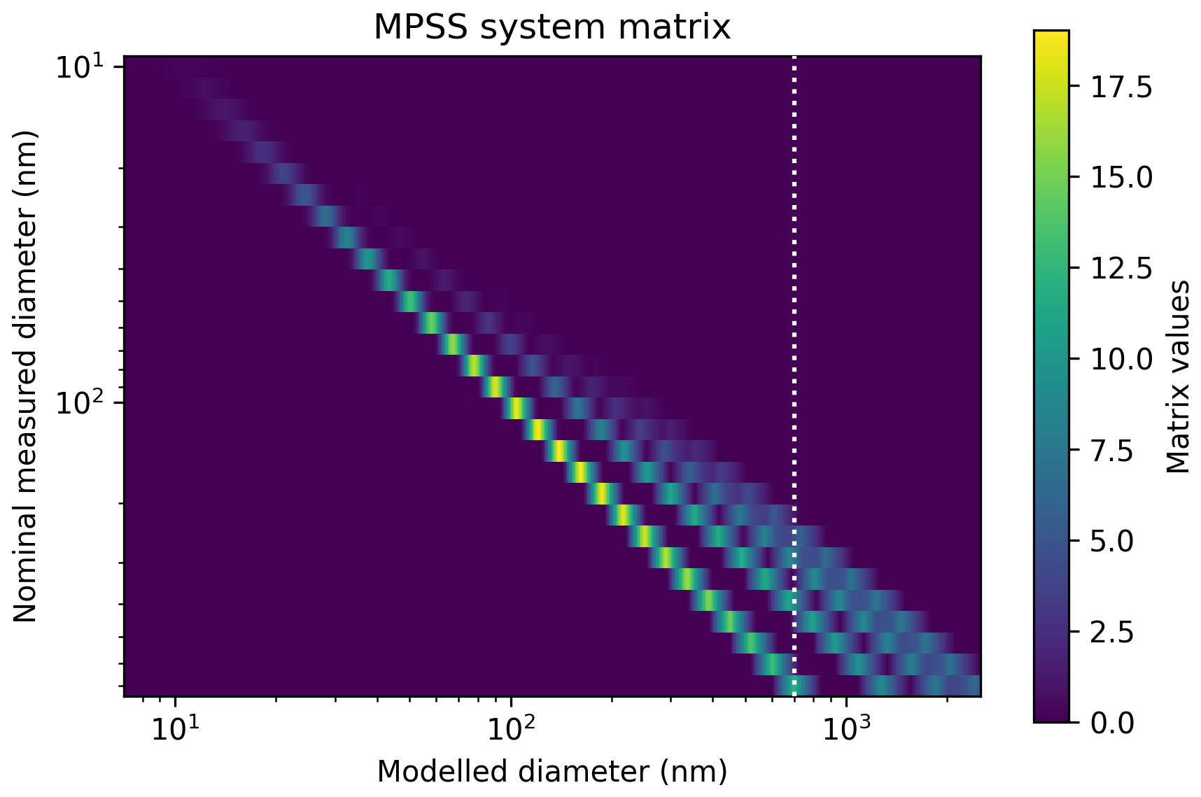
Figure 3 An example of an instrument matrix A (cf. Eq. 4) with up to 4 multiple charges modelled. The y-axis corresponds to the measured channels and the x-axis to the (discretization of) the modelled PSD. The white dotted line shows the size of the largest measured channel on the x-axis.

The grid $\mathit{\{}{\mathit{\nu }}_j{\mathit{\}}}_{j=\mathrm{1}}^J$ of ion mobilities used for marginalization is constructed so that the spacing in both the Z⁺ and Z⁻ directions is as uniform as possible, while dividing the region R into equal segments along each axis. The default grid spacing in MPSS-UQ is 0.035 ${\mathrm{cm}}^{\mathrm{2}}{\mathrm{V}}^{-\mathrm{1}}{\mathrm{s}}^{-\mathrm{1}}$, leading to 398 grid points. We verified the stability of posterior summaries at this discretization level with grid refinement, but denser grids can be used if required, with the usual accuracy-runtime trade-off.

In MPSS-UQ, each non-marginalized posterior is stored as the mean and covariance of its Laplace approximation, whereas the marginalized posteriors are stored as the samples drawn from the corresponding mixture distribution. For a modest number of posterior samples (thousands of draws), this requires less disk space than storing the full covariance matrices of each mixture component, while still being sufficiently accurate for posterior summaries. Further, storing the result as posterior samples retains the possibility to calculate posterior quantities, such as credible intervals or derived metrics, at different probability levels without having to re-run the inversion.

For datasets consisting of many independent measurements (e.g. time series), MPSS-UQ can distribute the inversions across available CPU cores. This parallel execution does not alter the statistical model or the posterior computation but can significantly reduce total computation time for large datasets.

4 Numerical and experimental validation of MPSS-UQ

In this section, we will carry out example inversions with MPSS-UQ. We start with simulated measurements to validate the proposed inversion approach, and then analyze a dataset of real DMPS measurements. To demonstrate the robustness of the proposed inversion approach, we calculate all results in this section with the same prior for x (with the parameters given in Sect. 3.1), not adjusting it based on, for example, the magnitude of the true particle number concentration. All results are also calculated using the LYF charging model, with the ion mobilities (values or whether they are marginalized) stated case by case.

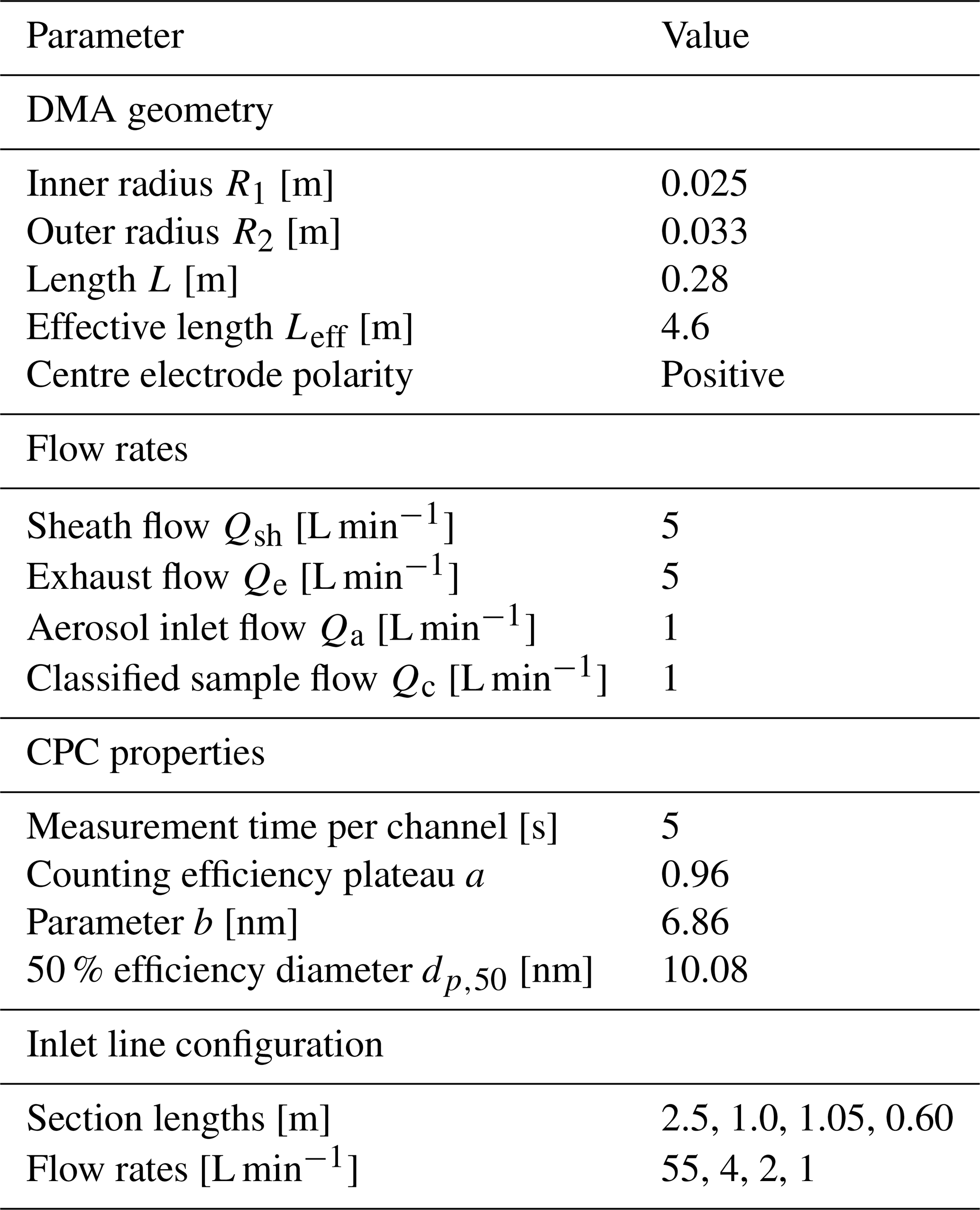
Both the synthetic datasets and the real measurements analyzed later are processed with the same instrument model. The DMPS transfer functions, diffusion losses, and CPC counting efficiencies were implemented as described in Appendix A. The sampling line connecting the aerosol inlet to the DMA consists of several tubing sections with different lengths and flow rates, corresponding to the actual setup used with the real measurements. The inlet layout as well as other instrument parameters are summarised in Table 2. A complete configuration file is also provided in the MPSS-UQ code repository.

Table 2 Key parameters of the DMPS model used for both simulated and real measurements. A complete configuration file is provided in the MPSS-UQ code repository.

4.1 Simulated measurements

To test the inversion on realistic simulated cases, MPSS-UQ implements the model aerosol distributions from Table 8.3 of Seinfeld and Pandis (2016, p. 343). These distributions are given as the sum of three lognormal modes, and represent a wide variety of aerosol distributions, ranging from the nearly particle-free “Polar” scenario to the high particle concentration “Urban” scenario. In addition, we include manually constructed size distributions that cannot be represented as a sum of lognormal modes, such as distributions with asymmetric or irregular shapes.

The simulated measurements are generated with the following general procedure. For all simulations, the ambient temperature and pressure are set to 293.15 K and 101 325 Pa, respectively, and the number of multiple charges modelled is 10. We represent the true PSD over the range [1, 2500] nm and discretize it into 500 logarithmically spaced bins, while the DMPS model is set to output 30 measurements at nominal diameters between 10 and 800 nm, also spaced logarithmically.

We first generate the noiseless expected counts $\stackrel{\mathrm{̃}}{\mathit{y}}=h\left(\mathit{x}\right)$ using Eq. (12). To model the errors that scale with particle concentration, we perturb the expected counts as ${\stackrel{\mathrm{̃}}{\mathit{y}}}^{\prime }=\stackrel{\mathrm{̃}}{\mathit{y}}\circ (\mathrm{1}+\mathit{\alpha }\mathit{\xi })$, where $\mathit{\xi }\sim \mathcal{N}(\mathrm{0},\mathbf{I})$ and ∘ denotes elementwise multiplication. We then simulate the discrete counting process of the CPC. The total expected count rate includes contributions from both the classified aerosol sample and a constant background rate λ_b=β², representing false counts from, e.g., homogeneous nucleation or detector noise. Since all individual detection events are independent, the total count follows a Poisson distribution:

$$\begin{array}{}\text{(34)}& \mathit{y}=\mathrm{Poisson}\left(max\left({\stackrel{\mathrm{̃}}{\mathit{y}}}^{\prime },\mathrm{0}\right)+{\mathit{\lambda }}_{\mathrm{b}}\right).\end{array}$$

The background rate λ_b=β² is chosen so that its Poisson variance matches the background variance β² in the observation model Eq. (18). Specifically, here we set α=0.01 and β²=0.1. Note that for computational convenience the observation model used in the inversion approximates the Poisson counting noise as Gaussian and evaluates the noise statistics at the observed counts y instead of at the true expected counts $\stackrel{\mathrm{̃}}{\mathit{y}}$.

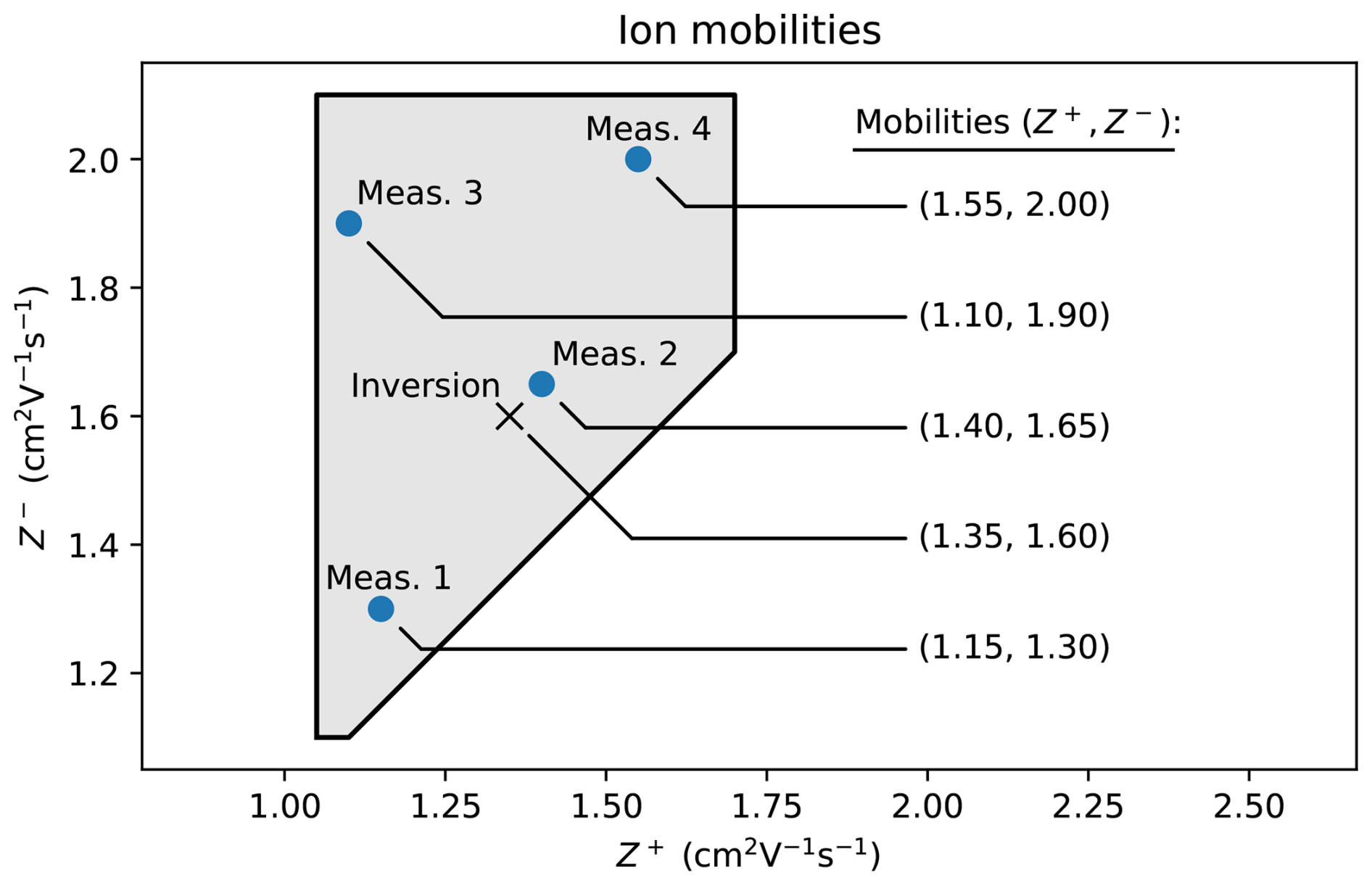
Figure 4 Ion mobilities used to generate the simulated measurements 1–4 and the mobility assumed when computing the MAP estimates.

When inverting synthetic measurements, we must take care to avoid the inverse crime, i.e. the artificial improvement in inversion performance that occurs when the same forward model and discretization are used both to generate and to invert the data (Kaipio and Somersalo, 2005). To prevent this, we lower the discretization used in the inversion to 100 logarithmically spaced bins, over the size range that is chosen automatically as described in Sect. 3.5. Note that the inversion is not very sensitive to the precise discretization as long as it is sufficiently dense. This can be verified by increasing the number of bins until the result does not change anymore. Further, during inversion we reduce the maximum modeled number of multiple charges from 10 to 8. These changes to the forward model, and approximating the Poisson + Gaussian additive noise as Gaussian in the likelihood, ensure that the inversion model is numerically and statistically different from the data-generation model and the inverse crime is avoided.

4.1.1 Effect of marginalization

Given that the main contribution of this paper is the quantification of charging-related uncertainty, let us first demonstrate the danger of not taking it into account. We simulate four DMPS measurements of the same PSD (the “Urban” aerosol distribution in Seinfeld and Pandis, 2016), which differ only in the assumed mobilities Z^± at the time of the measurement. We choose the ion mobilities so that they represent different but plausible measurement conditions over the polygon R, shown as blue dots in Fig. 4. The figure also gives the numerical values of the chosen mobilities.

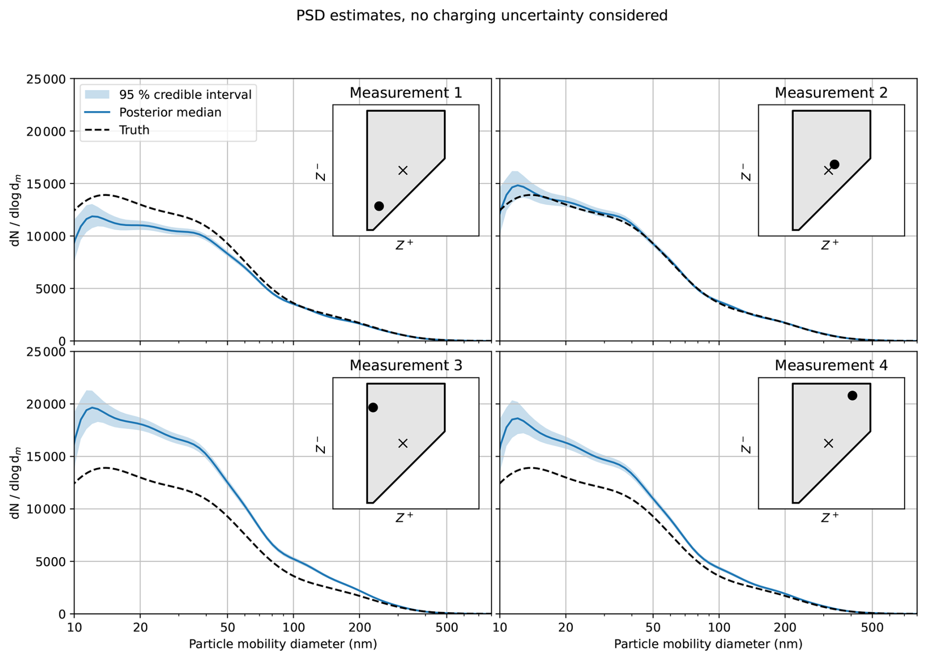
Figure 5 Estimated PSDs in the four synthetic data cases without considering the charging probability uncertainty. In the inset plot (cf. Fig. 4) the symbol • denotes the mobilities used in data generation and × denotes the mobilities used in the inversion.

We then compute the Laplace approximation in all four cases. Since in a real measurement the ion mobilities are typically not known, the usual practice at this point is to use a fixed charging probability, typically given by the Wiedensohler approximation. To mirror this practice here with the LYF model, we set $Z_{\mathrm{inv}}=(\mathrm{1.35},\mathrm{1.60})$ ${\mathrm{cm}}^{\mathrm{2}}{\mathrm{V}}^{-\mathrm{1}}{\mathrm{s}}^{-\mathrm{1}}$, which are the values the Wiedensohler approximation is based on (Wiedensohler, 1988). Figure 5 shows the resulting estimates. The charging probability clearly has a significant effect on the estimated PSD, and only in Measurement 2 where the ion mobilities during data generation happen to be close to Z_inv does the true PSD fall within the reported 95 % credible interval. For the other three cases, the PSD below 200 nm is either severely under- or overestimated and the true PSD lies outside the posterior support. This shows that treating the ion mobility as known leads to overly narrow posterior intervals or, in other words, the non-marginalized analysis is overconfident.

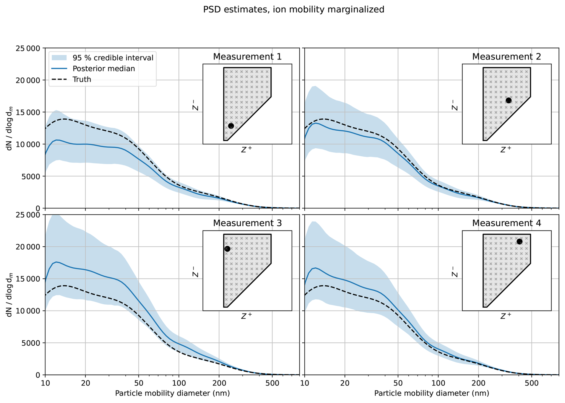
Figure 6 Estimated PSDs in the four synthetic data cases with the charging accounted for by marginalizing over the plausible ion mobilities. In the inset plot, • denotes the mobilities used in data generation and multiple ×s illustrate the idea that the whole mobility range is considered in the marginalization. Note that the number of the mobilities considered during marginalization is a lot higher than in this schematic.

Now we repeat the inversion but marginalize over the ion mobility. The results are shown in Fig. 6. Again, the posterior medians still vary with the measurement conditions, though less than in the non-marginalized case. More importantly, the resulting 95 % credible intervals are much wider and, crucially, they contain the true PSD in all four cases. The wider intervals reflect the uncertainty introduced by the unknown mobilities, and therefore provide a more realistic representation of the uncertainty in this inference problem.

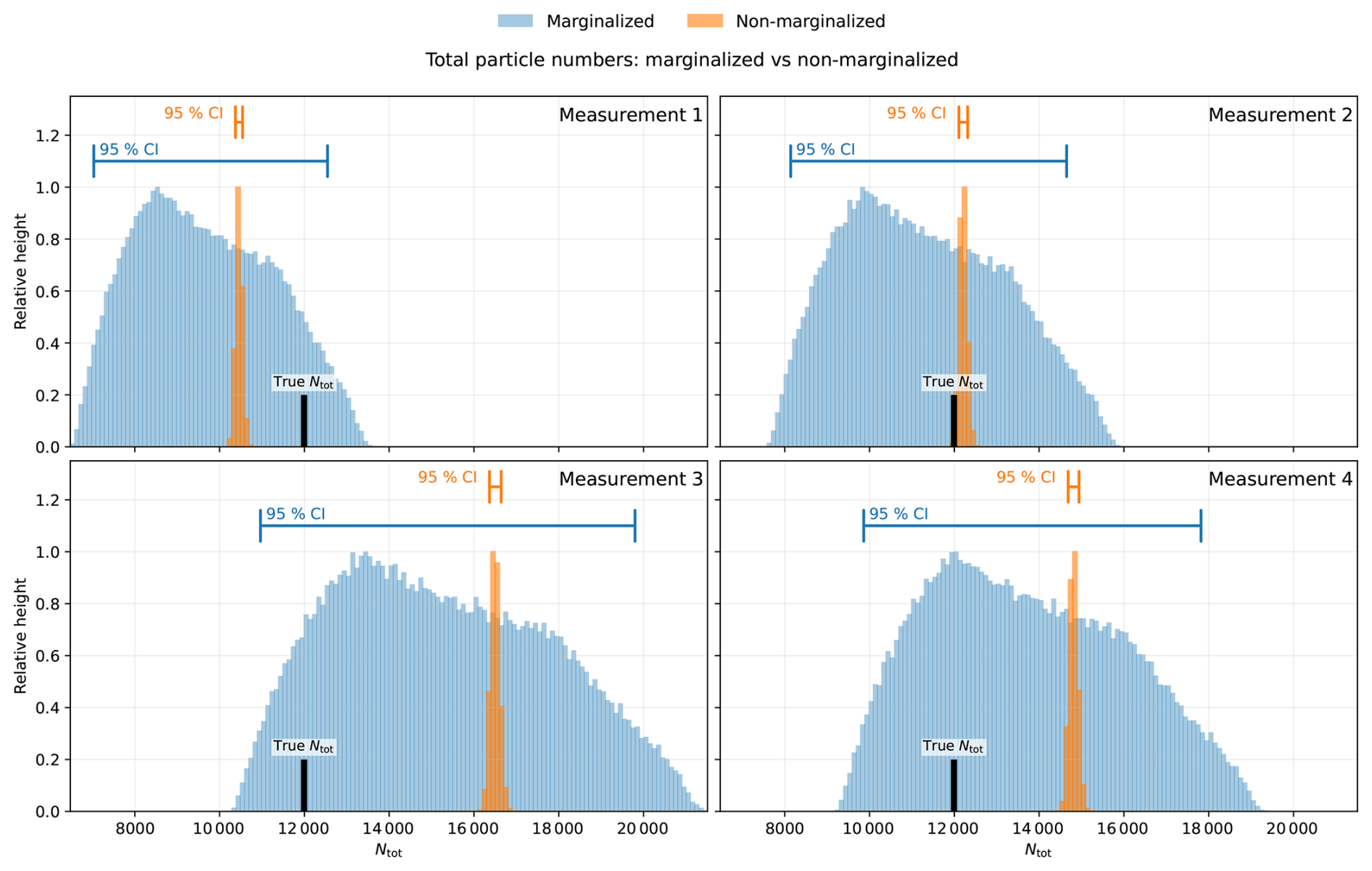
Figure 7 Histograms of the total particle numbers N_tot based on the marginalized and non-marginalized inversion results for the “Urban” aerosol distribution. The histograms are scaled so that their maximum bin =1. The horizontal bars depict the 95 % credible intervals. Also shown is the true N_tot.

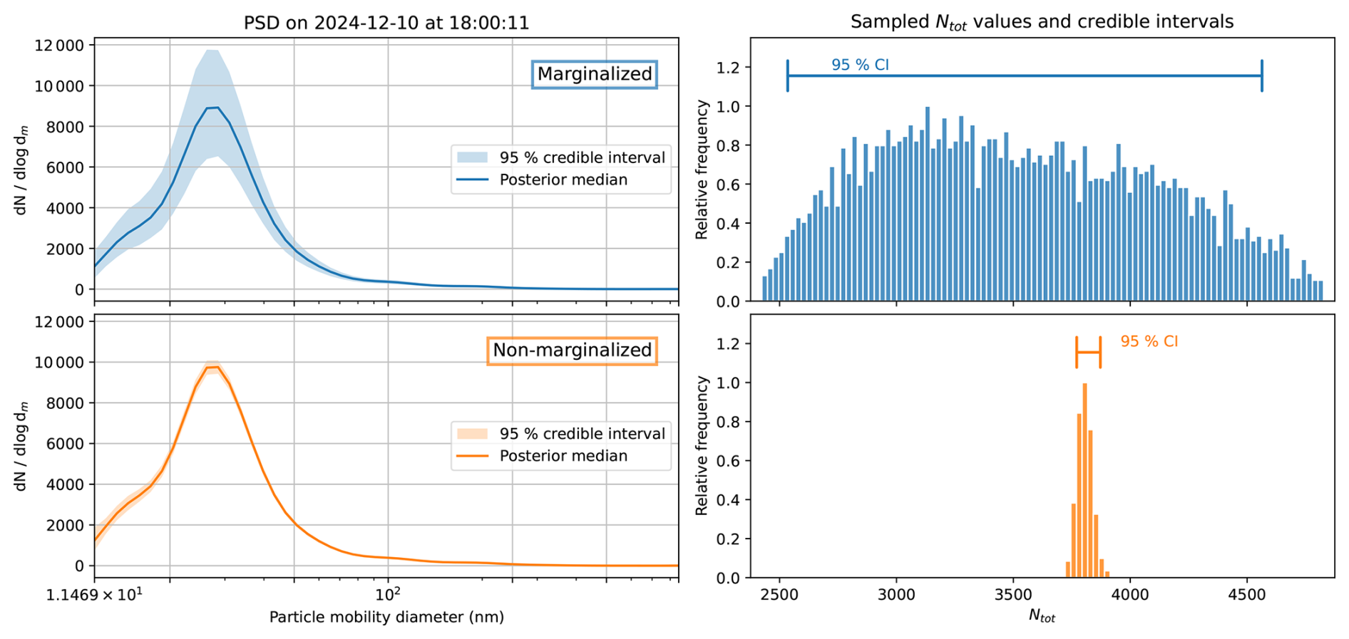
The difference between the non-marginalized and the marginalized inversions appears perhaps even more clearly in the total particle number, $N_{\mathrm{tot}}={\sum }_j{N}_j$, which (as a function of the PSD) inherits uncertainty from the posterior distribution of the PSD. To quantify this, we draw posterior samples of the PSD, compute the corresponding values of N_tot, and summarize their distribution. Figure 7 shows histograms of N_tot for each of the four measurements, in both the marginalized and non-marginalized cases, along with the true N_tot and the 95 % credible intervals. When the charging uncertainty is included, the credible intervals in this example are 18–21 times wider than when the ion mobilities are fixed. As with the PSD estimates, the true total particle number lies within the posterior credible intervals only in Measurement 2 and the marginalized cases.

4.1.2 Different types of aerosol distributions

Let us now apply the inversion method to other aerosol scenarios, namely “Rural”, “Remote continental”, “Rural” scaled down to $\mathrm{1}/\mathrm{10}$th of its concentration, and “Polar” all taken from Table 8.3 of Seinfeld and Pandis (2016, p. 343), and to manually created scenarios which model a trimodal nucleation event, an asymmetric mode, and an irregularly shaped distribution where broad modes are modified by an AR(1) process. These cases, including the unrealistic irregular scenario, cover a wide range of modal structures and particle concentration levels, which allows the evaluation of how the method behaves across these different PSD shapes. In all of these tests we marginalize the charging probability. To isolate the effect of the PSD shape, all synthetic measurements in this subsection are generated using the same charging ion mobilities, $Z_{\mathrm{inv}}=(\mathrm{1.35},\mathrm{1.60})$ ${\mathrm{cm}}^{\mathrm{2}}{\mathrm{V}}^{-\mathrm{1}}{\mathrm{s}}^{-\mathrm{1}}$, and the prior for x is identical to that of the previous subsection. For each scenario, we show the posterior median PSD together with its 95 % credible interval and compare it against the true distribution.

Figure 8 Marginalized posteriors for various simulated aerosol distribution scenarios.

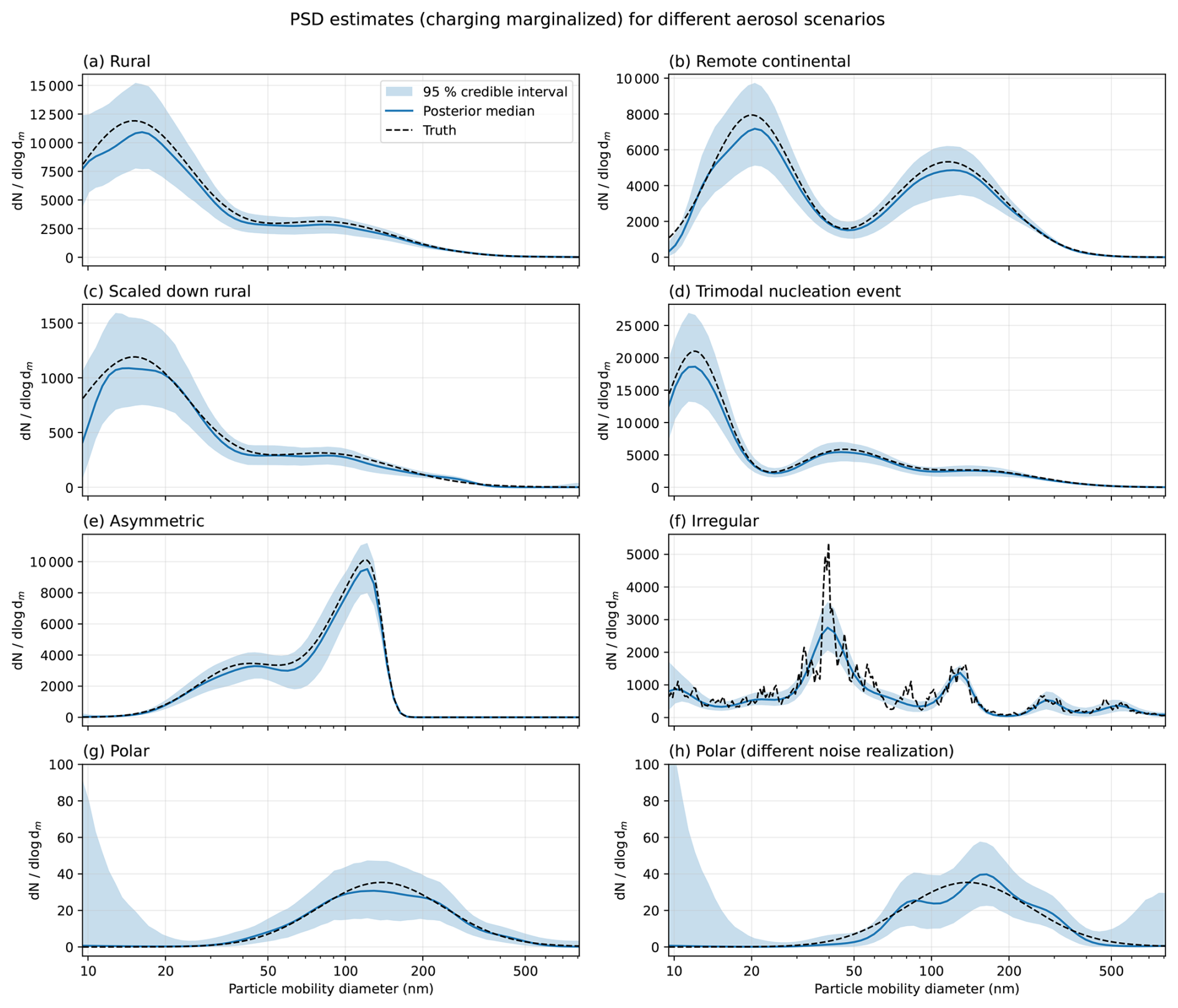
Figure 8a–h show the inversion results. Note that in none of the tested scenarios do we expect the posterior median to coincide exactly with the true PSD, as this would require either knowing the true ion mobilities or, by chance, that the true mobilities and the effective values implied by the marginalization matched. With this in mind, across most scenarios the method successfully estimates the main modal structure and the true PSD is found within the credible intervals. The one exception is the irregular scenario (f) where the credible intervals do not cover the sharp peaks. This is expected given the size-resolution of the DMPS and the fact that such jumps are neither realistic nor supported by the smoothness prior. However, the overall shape of the size distribution is estimated correctly. Comparison between the “Rural” scenario and its scaled down counterpart in panels (a) and (c) shows that the lower signal-to-noise ratio in scenario (c) results in slightly wider credible intervals relative to the median estimate. Finally, to demonstrate the effect of random noise on the estimates, panels (g) and (h) both show the same low-concentration “Polar” scenario, which has the lowest signal-to-noise-ratio of the tested cases. The panels differ only in the realization of measurement noise (see Eq. 34). Because the signal-to-noise ratio is low, the likelihood constrains the posterior only weakly, and different noise realizations lead to noticeably different posterior shapes even though the broad shape of the PSD is still recovered. These results indicate that the proposed Bayesian approach works across a wide variety of aerosol size distributions without the need for fine-tuning.

4.2 Real measurements

As a preliminary verification, we applied MPSS-UQ to raw count data from a commercial SMPS system (TSI Inc. electronic classifier model 3082 coupled with TSI 3776 ultrafine CPC) measuring an atmospheric simulation chamber, using the Wiedensohler charging probability approximation. The posterior median PSDs recovered by MPSS-UQ agree with the standard TSI inversion in both shape and magnitude (not shown), confirming that the proposed method produces results consistent with an established reference when the same charging model is used. Despite the fact that the two approaches likely differ in their implementation of the SMPS forward model, the majority of the TSI point estimates fall within the MPSS-UQ 95 % credible intervals.

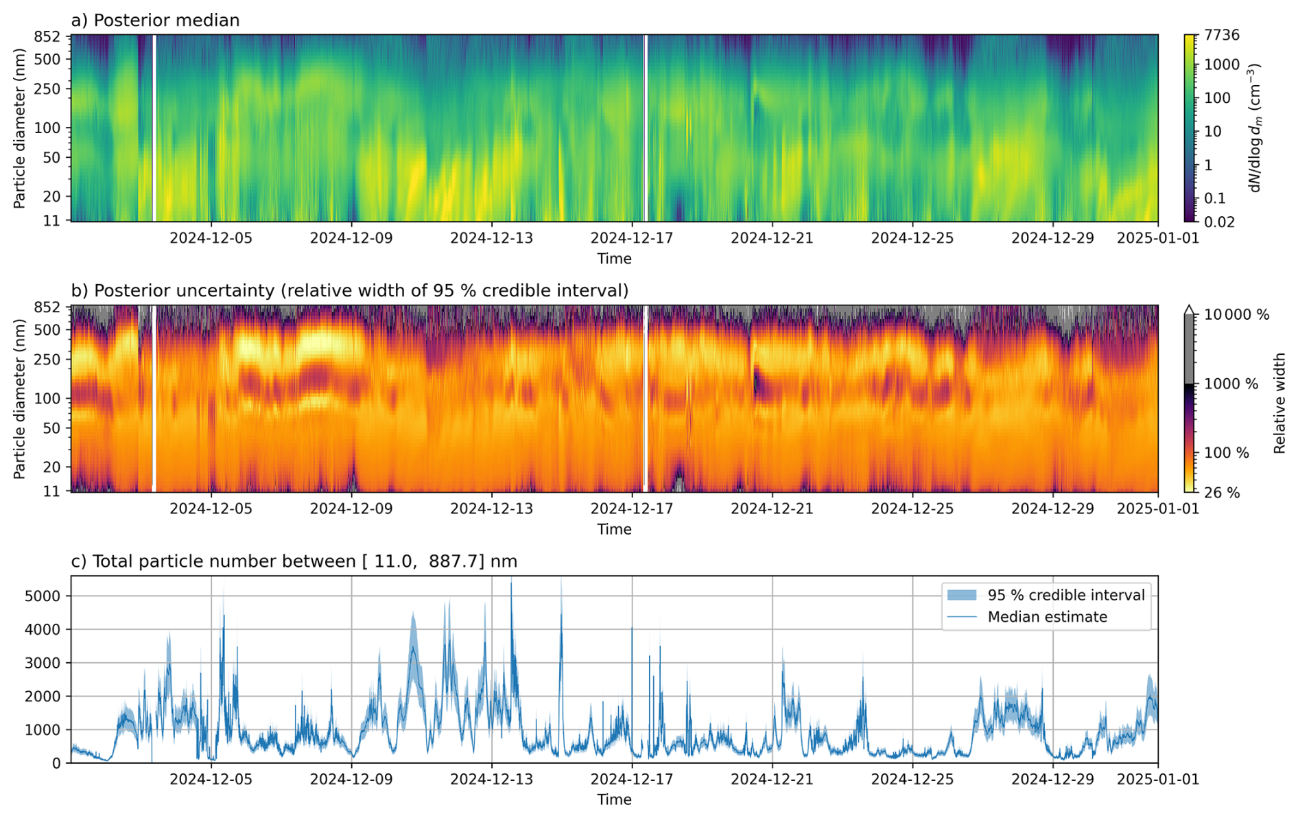
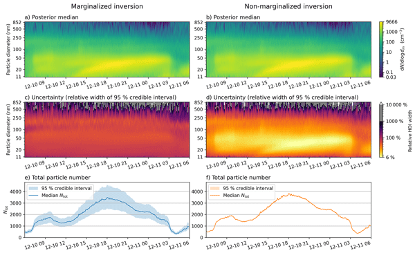
Figure 9 Month-long results for December 2024 using the marginalized inversion. (a) Posterior median PSD, $\widehat{\mathbf{N}}$. (b) Relative uncertainty $W=({\mathrm{CI}}_{\mathrm{95},\mathrm{high}}-{\mathrm{CI}}_{\mathrm{95},\mathrm{low}})/\widehat{\mathbf{N}}$. (c) Total particle number N_tot with 95 % credible interval.

We now apply the MPSS-UQ inversion to field data from a month-long DMPS deployment in December 2024 at the Puijo measurement station in Kuopio, Finland, where the charging probability is no longer assumed known and the full marginalization is used. The DMPS consists of a Nickel-63 charger, a Vienna-type cylindrical DMA operated with a closed-loop sheath flow, and an Airmodus A20 CPC. The instrument configuration and parameters are summarized in Table 2. The DMPS is set to measure 29 logarithmically spaced channels between nominal diameters of 11.6 and 800 nm, and in the inversion we use 70 size bins. The whole size range is measured every 6 min resulting in approximately 7400 scans. Temperature and pressure were recorded for each scan, and they are used to update the DMPS instrument matrix during inversion at every scan.

The full marginalization of the entire dataset with MPSS-UQ required about 10 min on a standard laptop (Intel(R) Core(TM) i7-12700H processor, 32 GB RAM). Figure 9 displays the posterior median PSD (panel a), the associated relative uncertainty (panel b), and the total particle number time series (panel c). The white vertical gaps correspond to instrument maintenance periods. We quantify the uncertainty as the relative width of the 95 % highest density credible interval,

$$\begin{array}{}\text{(35)}& W={\displaystyle \frac{{\mathrm{CI}}_{\mathrm{95},\mathrm{high}}-{\mathrm{CI}}_{\mathrm{95},\mathrm{low}}}{\widehat{\mathbf{N}}}}\cdot \mathrm{100}\mathit{\%},\end{array}$$

where ${\mathrm{CI}}_{\mathrm{95}}=[{\mathrm{CI}}_{\mathrm{95},\mathrm{low}},{\mathrm{CI}}_{\mathrm{95},\mathrm{high}}]$ denotes the 95 % credible interval and $\widehat{\mathbf{N}}$ the posterior median. We report relative rather than absolute uncertainty because MPSS measurements follow a Poisson counting process whose standard deviation grows with the expected count as $\sqrt{\stackrel{\mathrm{̃}}{y}}$. As a consequence, the absolute posterior uncertainties are roughly proportional to concentration, so that an absolute uncertainty plot is visually similar to the median estimate itself and therefore conveys little additional information. The relative width W removes this scaling: a value of W=100 % always means that the width of the 95 % credible interval equals the posterior median, regardless of the concentration level. This makes W an interpretable and scale-independent measure of uncertainty that is consistent with both the Poisson noise model and the log ₁₀-scale parametrization of the PSD. Note that the colour scale in panel (b) is divided into three regions to accommodate the wide dynamic range of W. For W≤1000 %, the color map shows full contrast in the range where the data most meaningfully constrain the PSD. Values between 1000 % $<W\le \mathrm{10}\mathrm{000}$ % are shown in grey to indicate a zone where the posterior is narrower than the prior but the estimate remains highly uncertain. Values exceeding W=10 000 %, where the data provide little constraint beyond the prior, are shown in white. Finally, panel (c) shows the total particle number concentration together with its 95 % credible interval. We discuss some more derived quantities in Sect. 5.

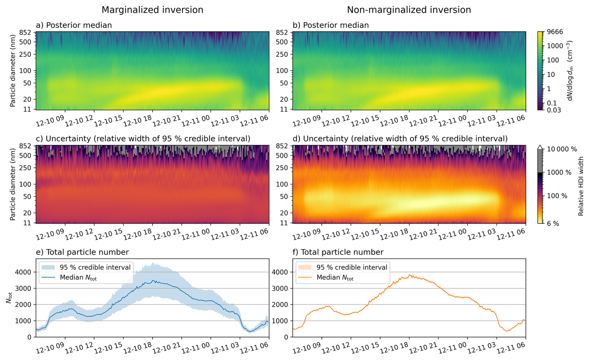
Figure 10 Example day 1 (10–11 December 2024, 06:00 am to 06:00 a.m. LT): comparison of marginalized and fixed-mobility (non-marginalized) inversions. (a–b) Posterior median PSDs. (c–d) Relative credible-interval width W. (e–f) Total particle number N_tot with 95 % credible intervals. Time axes are aligned across all panels.

Multiple new particle formation (NPF) events, as well as days with low particle concentrations, are visible in the month-long dataset. To examine differences between the marginalized and fixed-mobility inversions in detail, we analyze two representative days: an NPF event on 10 December 2024 and a low-concentration day on 25 December 2024.

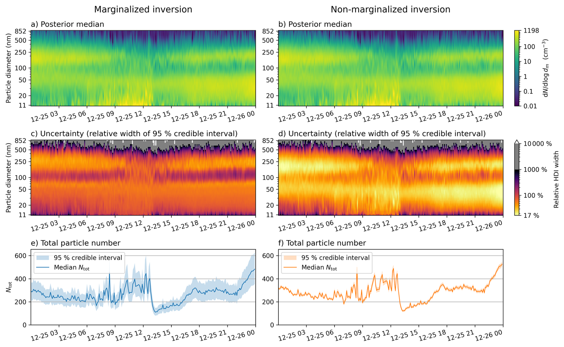
Figure 11 Example day 2 (25 December 2024): comparison of marginalized and fixed-mobility inversions. (a–b) Posterior median PSDs. (c–d) Relative uncertainty width W. (e–f) Total particle number N_tot with 95 % credible intervals.

Figure 10 shows the inversion results for the NPF event day. The posterior median PSDs in panels (a) and (b) differ only slightly between the two approaches, but this is expected: the posterior median of the marginalized inversion corresponds approximately to using an “effective” set of charging probabilities averaged over the mobility prior region R, and the fixed mobilities used in the non-marginalized inversion lie near the center of this region. The relative credible interval widths W (shown in panels c and d), however, are considerably larger in the marginalized case than in the non-marginalized one. The ratio of W between the marginalized and non-marginalized inversions ranges from 1 to 9 across the measured size range. Further, the non-marginalized intervals suggest there is a band from roughly 20 to 70 nm, corresponding to bins with the highest concentration of particles, that has much less uncertainty than the surrounding sizes. The marginalized intervals do not support this, however, and instead they indicate that the uncertainty is roughly constant between 20 and 250 nm, increasing only slightly towards smaller sizes. As with the synthetic data examples earlier, the differences are most apparent in total particle numbers N_tot (panels e and f). While the posterior medians of N_tot are similar, the ratio of marginalized to fixed 95 % credible interval widths varies between 4 and 18.

Figure 11 shows the results for the low-concentration day. The qualitative differences between the two inversion approaches remain the same, but the ratios are somewhat smaller: the W ratio varies between 1 and 4 across the size range, and the corresponding N_tot credible interval width ratio varies between 3 and 8, compared with 1–9 and 4–18 for the NPF day, respectively. This is consistent with a general pattern across the full dataset, where the ratio increases with total particle number concentration (correlation r=0.78). In other words, the degree to which the fixed-mobility inversion underestimates the uncertainty grows with concentration.

To illustrate inversion output at the level of a single measurement, Fig. 12 presents the posterior median and 95 % credible intervals for one scan from the NPF event. The difference between the marginalized and fixed-mobility credible intervals is clearly visible, consistent with the patterns observed in the full-day results above.

Figure 12 Inversion results for a single scan during the NPF event on 10 December 2024.

5 Discussion

The accuracy of an MPSS measurement depends on all of its components: the bipolar charger, the DMA, and the CPC, for which recommended calibration procedures exist. For example, a successfully calibrated MPSS is expected to agree with a reference instrument to within ±10 % in the 20–200 nm range and ±20 % between 200 and 800 nm (Wiedensohler et al., 2017). However, these benchmarks are established under controlled laboratory conditions where the candidate and reference instruments share the same environment and carrier gas composition. Since the charging ion mobilities depend on the carrier gas, such inter-comparisons are not sensitive to charger-related uncertainty. In field deployments, where the carrier gas composition may vary and is generally not monitored, the actual uncertainty can be much larger than these calibration benchmarks suggest. Our results show that when the charging probability is considered to be uncertain in the inversion and allowed to vary within physically justified bounds, the resulting posterior credible intervals are indeed far wider than those obtained by treating the ion mobility as known. Specifically, taking the month-long dataset (see Sect. 4.2) as an example, we found that in the marginalized case the relative widths of the 95 % credible intervals are typically 1 to 10 times larger with a mean of 2.4, compared to the fixed charging probability case. These values are consistent with the sensitivity analysis presented in Leppä et al. (2017). For the total particle number we found that the corresponding credible interval widths were 3 to 18 times larger with a mean of 8.5. Both ratios increase with concentration level, which means that the fixed-mobility inversion underestimates uncertainty the most where the data are most informative. This highlights one of the strengths of the presented approach: it provides systematic, measurement- and size-specific uncertainty estimates of each inverted size distribution. Further, since the marginalized inversion accounts for a physically important source of uncertainty that the conventional approach ignores, its wider credible intervals represent a more realistic characterization of what the instrument can resolve.

In practice, information from the uncertainty estimates can be used in several ways. First, the 95 % highest density intervals provide a justifiable range within which the PSD and any derived quantities should be interpreted. When these intervals are wide, conclusions drawn from the corresponding size range or time period should be treated with appropriate caution. For estimates (and credible intervals) that can span multiple orders of magnitude, the relative credible interval width W (Eq. 35) shows how strongly the data constrain the PSD at each size and time (see for example Fig. 9b). Regions with small W are well supported by the measurement, whereas regions with large W are only weakly constrained. This is particularly relevant when comparing measurements across days or sites, or when interpreting weak signals such as early-stage nucleation events. When the absolute magnitude of the uncertainty matters, for example, when assessing whether a concentration exceeds a specific threshold, the credible intervals themselves can be examined directly. This is also useful with very small number concentrations, where the relative width may be enormous but the absolute uncertainty still tiny. Finally, samples from the posterior can be propagated through any derived quantity, yielding uncertainty estimates that are not available from conventional inversion methods. Rather than computing a derived quantity from a single point estimate, one computes it for each posterior sample and obtains a distribution that reflects the full posterior uncertainty from which credible intervals can be computed.

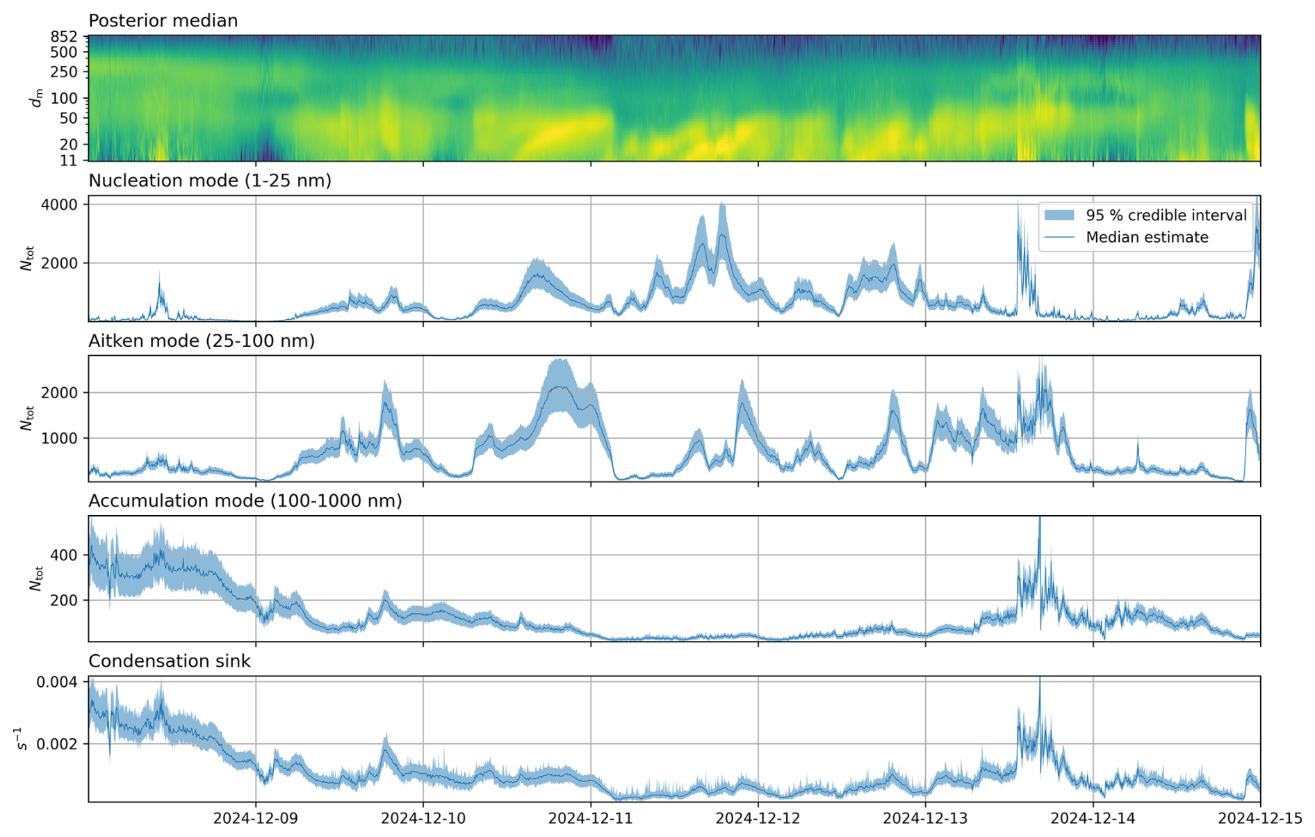
Figure 13 An example of a few derived quantities with uncertainties calculated from the estimated PSD. Shown are the total number concentrations of the nucleation mode, the Aitken mode, and the accumulation mode, as well as the sulfuric-acid vapour condensation sink.

To illustrate this, Fig. 13 shows one week worth of posterior distributions of several derived quantities obtained from the month-long dataset (the median PSD estimate is shown as the top row for easy reference): nucleation-mode concentration (d_p<25 nm), Aitken-mode concentration ($\mathrm{25}\le d_p<\mathrm{100}$ nm), accumulation-mode concentration (d_p≥100 nm), and the sulfuric-acid vapour condensation sink (gas-uptake rate, s⁻¹). For reference, the total particle number concentration N_tot is shown in Fig. 9c.

The nucleation-mode concentration deserves particular attention. Nucleation events are frequently identified and characterized using MPSS data, yet the sub-25 nm range is precisely where the charging efficiency is lowest and most uncertain. The credible intervals for the nucleation-mode concentration are correspondingly wide which indicates that conclusions about nucleation-mode particle numbers should be drawn with care.

Additional derived quantities implemented in MPSS-UQ include the geometric mean diameter, mode diameter, median diameter, surface area concentration, volume concentration, and effective diameter. We do not present results for these here, but they are readily available through the MPSS-UQ package for any dataset processed with the method.

5.1 Factors influencing the magnitude of uncertainty

To interpret the uncertainty plots, it is helpful to understand the main factors that determine the width of the posterior credible intervals.

The factor that has the most straightforward effect is the particle concentration level. Because particle counting follows Poisson statistics, relative counting noise decreases as the count rate increases. Higher concentrations therefore provide more informative measurements and lead to tighter posteriors than do low concentrations. This is visible in the relative uncertainty plots, where the smallest concentrations typically correspond to the highest values of W.

Several physical effects reduce inversion accuracy at the edges of the size range. Charging efficiency drops rapidly below roughly 20 nm, the proportion of multiply charged particles becomes more significant at larger diameters, and sub-20 nm particles additionally suffer stronger diffusion losses that reduce the number that reach the CPC. Together, these effects make the smallest and largest bins more weakly constrained and lead to wider credible intervals in those regions.

A factor particularly relevant to the present work is the assumed range of ion mobilities. The width of the mobility prior region R determines how much charging-related uncertainty enters the inference. A narrower R, i.e., better prior knowledge of ion mobilities (for example through tighter control of carrier gas composition, or even directly measuring the ion properties) results in correspondingly narrower posterior credible intervals. In the limiting case where ion mobility is treated as known, the marginalised posterior collapses to the non-marginalised one, which reproduces the narrow, but typically overconfident, intervals shown in Sect. 4.

The size resolution and number of measurement channels also play a role. The amount of independent information available from the data depends on the number, spacing, and width of the channels. Instruments with more channels per scan, such as a typical SMPS compared to a typical DMPS, may support finer structure in the inferred PSD, provided the prior correlation length is adjusted accordingly. For example, in the SMPS verification we used a correlation length of l=0.25 decades while still obtaining smooth, realistic results, whereas the sparser DMPS data required l=0.5 decades to avoid fitting noise.

5.2 Limitations

Let us now discuss some limitations of the present work.

First, the inversion presented here treats each measurement scan independently, without modelling temporal correlations between successive scans. In reality, the PSD evolves continuously, and consecutive scans are not independent. A temporal model, for example based on Kalman filtering or smoothing (Voutilainen and Kaipio, 2001; Viskari et al., 2012; Ozon et al., 2021), could exploit this continuity to further constrain and smooth the posterior estimates. Extending the current framework to include temporal dependence is a natural direction for future work.

The present work focuses on charging probability as the dominant source of model uncertainty, but other factors also contribute, including uncertainties in the DMA transfer function, CPC counting efficiency, flow rates, and particle losses in the sampling lines. These could in principle be incorporated into the Bayesian framework as additional nuisance parameters to be marginalized, though the computational cost increases with each added parameter and may quickly become prohibitive. The effect of additional sources of uncertainty could potentially be taken into account in an approximate manner using the Bayesian approximation error approach (Kaipio and Somersalo, 2007; Kaipio and Kolehmainen, 2013), which accounts for model uncertainties by statistically characterizing their effect on the observations and including them into the likelihood. This would allow additional sources of uncertainty to be included at a fraction of the computational cost of full marginalization. A systematic comparison of the relative contributions of the sources of uncertainty (cf. Coquelin et al., 2018) would help prioritize which ones merit explicit treatment and which can be treated, e.g., with approximate methods.

As discussed in Sect. 2.2, there are several models available for describing bipolar charging kinetics (López-Yglesias and Flagan, 2013; Gatti and Kortshagen, 2008; Gopalakrishnan et al., 2013), and all results presented in this work are conditioned on the validity of the chosen LYF model (López-Yglesias and Flagan, 2013). The Bayesian framework itself, however, is not tied to this particular model and any charging model that maps ion properties to charge fractions can be substituted without changes to the inversion methodology. The LYF model, like all charging models, includes approximations and uncertainties in its description of the charging process, such as the assumption that the particles are spherical or that each ion-particle collision results in a charge transfer (Leppä et al., 2017). The model also requires input parameters other than the ion mobilities (and masses), such as the relative permittivities of the particles and ions (χ_p=80 and χ_i=5 in this work), which we have taken as fixed here but which can also introduce additional bias, especially for particles composed of low-permittivity materials (Leppä et al., 2017). We have also assumed that the concentrations of positive and negative charger ions are equal, although a charge imbalance can arise from the higher wall-loss rate of the more mobile negative ions in the plumbing downstream of the charger (Tigges et al., 2015). Marginalization over this parameter is implemented in MPSS-UQ but was not explored in this study.

Finally, in the treatment of charging uncertainty in this work we approximated the ion properties as single values of positive and negative mobility, whereas in reality the charging environment contains a mixture of ion species with different masses, mobilities, and structures. Both ambient mass spectrometric measurements (Ehn et al., 2010) and laboratory tandem mobility–mass analyses of radioactive source ions (Maißer et al., 2015) have shown that the ion population is chemically diverse, temporally variable, and system-dependent. The standard Fuchs charging equations can be extended to account for such distributions of bipolar ion mobilities (Lee et al., 2005), and the resulting charging ratios can differ from those computed using a single ion type. In the context of the present work, this means that the true charging-related uncertainty may be broader than what our two-parameter marginalization over $(Z^{+},Z^{-})$ captures, since it does not account for the polydispersity of the ion population itself. A more realistic representation of the ion mobility distribution in the marginalization is a natural extension of this work, though it would require reliable characterization of the ion population under the specific charger and gas conditions used, which remains a considerable experimental challenge.

6 Conclusions

Electrical mobility-based measurements of aerosol size distributions are widely used in atmospheric science, yet the uncertainty introduced by imprecisely known charging probability is rarely quantified or reported. In this work, we developed a Bayesian inversion approach that systematically accounts for this uncertainty by treating the charger ion mobilities as nuisance parameters and marginalizing over their physically plausible range. The resulting credible intervals provide an honest characterization of what the instrument can and cannot resolve, conditional on the model assumptions. Further, the approach enables straightforward propagation of uncertainty to any derived quantity, such as total particle number, through evaluation over posterior samples.

The method was validated on synthetic data covering a wide range of aerosol scenarios and then applied to a month-long field dataset from a DMPS deployed at the Puijo measurement station in Kuopio, Finland. We found that in this dataset, marginalizing over the uncertain ion mobilities widens the posterior credible intervals by a mean factor of 2.4 compared to conditioning on fixed mobility values, with widening factors up to 10 in some size and time ranges. The ratio of marginalized to fixed-mobility credible interval widths for the total particle number concentration ranged from 3 to 18 depending on concentration level, which shows that conventional inversions that condition on fixed ion mobilities can substantially underestimate uncertainty.

The method is implemented in the open-source Python package MPSS-UQ (Niskanen, 2026), which is freely available on GitHub. The package provides the full inversion pipeline, including the marginalization over charging probability, posterior sampling, and uncertainty propagation to derived quantities. Even if the full marginalization is not carried out, the sensitivity of results to assumptions about the charging probability can still be assessed. Processing a month of DMPS data (∼7400 scans), as an example, requires approximately 10 min on a standard laptop when carrying out the marginalization and much less if performing inversions with a single charging probability assumed. This should make routine uncertainty quantification practical for both campaign and long-term monitoring datasets. The availability of uncertainty estimates should enable more rigorous comparison between instruments, sites, and time periods, and support the propagation of measurement uncertainty into downstream analyses such as emission source attribution, climate modelling, and health impact assessment.

Appendix A: Expressions of the MPSS formulas

A1 DMA transfer function

The DMA transfer function $T\left(Z\right(d,p),Z_i)$ describes the probability that a particle with mobility Z(d,p), where d is the diameter and p the charge, exits the DMA when it is set to measure the mobility Z_i. We adopt the model derived by Stolzenburg (1988) which accounts for diffusion in the particles due to Brownian motion, and assume here a cylindrical (axial flow) DMA. Define the dimensionless flow parameters

$$\begin{array}{}\text{(A1)}& \mathit{\beta }={\displaystyle \frac{Q_{\mathrm{a}}+Q_{\mathrm{c}}}{Q_{\mathrm{sh}}+Q_{\mathrm{e}}}},\mathit{\delta }={\displaystyle \frac{Q_{\mathrm{c}}-Q_{\mathrm{a}}}{Q_{\mathrm{c}}+Q_{\mathrm{a}}}},\end{array}$$

where $Q_{\mathrm{a}},Q_{\mathrm{c}},Q_{\mathrm{sh}}$, and Q_e are the rates of the aerosol flow, classified sample flow, sheath flow, and exhaust flow, respectively, and denote the ratio of the electrical mobility of the particle and the target electrical mobility by

$$\begin{array}{}\text{(A2)}& {\stackrel{\mathrm{̃}}{Z}}_p={\displaystyle \frac{Z(d,p)}{Z_i}}.\end{array}$$

The transfer function is then given by

$$\begin{array}{}\text{(A3)}& \begin{array}{rl}T\left({\stackrel{\mathrm{̃}}{Z}}_p\right)& ={\displaystyle \frac{\mathit{\sigma }}{\sqrt{\mathrm{2}}\mathit{\beta }(\mathrm{1}-\mathit{\delta })}}\left[\mathit{\epsilon }\left({\displaystyle \frac{{\stackrel{\mathrm{̃}}{Z}}_p-(\mathrm{1}+\mathit{\beta })}{\sqrt{\mathrm{2}}\mathit{\sigma }}}\right)\right.\\ & +\mathit{\epsilon }\left({\displaystyle \frac{{\stackrel{\mathrm{̃}}{Z}}_p-(\mathrm{1}-\mathit{\beta })}{\sqrt{\mathrm{2}}\mathit{\sigma }}}\right)-\mathit{\epsilon }\left({\displaystyle \frac{{\stackrel{\mathrm{̃}}{Z}}_p-(\mathrm{1}+\mathit{\beta }\mathit{\delta })}{\sqrt{\mathrm{2}}\mathit{\sigma }}}\right)\\ & \left.-\mathit{\epsilon }\left({\displaystyle \frac{{\stackrel{\mathrm{̃}}{Z}}_p-(\mathrm{1}-\mathit{\beta }\mathit{\delta })}{\sqrt{\mathrm{2}}\mathit{\sigma }}}\right)\right],\end{array}\end{array}$$

where $\mathit{\epsilon }\left(x\right)=x\mathrm{erf}\left(x\right)+e^{-x^{\mathrm{2}}}/\sqrt{\mathit{\pi }}$, erf(x) denotes the error function, and σ is given by

$$\begin{array}{}\text{(A4)}& {\mathit{\sigma }}^{\mathrm{2}}={\displaystyle \frac{G_{\mathrm{DMA}}{\stackrel{\mathrm{̃}}{Z}}_p}{Pe}}.\end{array}$$

Above, Pe is a migration Peclet number which for a cylindrical DMA is

$$\begin{array}{}\text{(A5)}& P{e}_{\mathrm{mig}}={\displaystyle \frac{\left|p\right|eV}{k_{\mathrm{B}}T}}{\displaystyle \frac{\mathrm{1}-\frac{R_{\mathrm{1}}}{R_{\mathrm{2}}}}{\ln \frac{R_{\mathrm{2}}}{R_{\mathrm{1}}}}},\end{array}$$

where e is the elementary charge, p is the number of charges, V is the target DMA voltage, k_B is the Boltzmann constant, T is the temperature, R₁ and R₂ denote the inner and outer radii of the DMA, respectively, and G_DMA is a geometry factor given by

$$\begin{array}{}\text{(A6)}& G_{\mathrm{DMA}}=\mathrm{4}{\displaystyle \frac{(\mathrm{1}+\mathit{\beta }{)}^{\mathrm{2}}}{\mathrm{1}-\mathit{\gamma }}}\left(I+\left(\mathrm{2}\right(\mathrm{1}+\mathit{\beta })\mathit{\kappa }{)}^{-\mathrm{2}}\right)\end{array}$$

with

$$\begin{array}{}\text{(A7)}& \mathit{\gamma }={\left({\displaystyle \frac{R_{\mathrm{1}}}{R_{\mathrm{2}}}}\right)}^{\mathrm{2}},I={\displaystyle \frac{\mathrm{1}+\mathit{\gamma }}{\mathrm{2}}},\mathit{\kappa }=L{\displaystyle \frac{R_{\mathrm{2}}}{R_{\mathrm{2}}^{\mathrm{2}}-R_{\mathrm{1}}^{\mathrm{2}}}},\end{array}$$

where L is the length of the DMA.

A2 Diffusion losses

We calculate the diffusion losses in sampling lines using a piecewise empirical approximation to the Gormley–Kennedy model (Gormley and Kennedy, 1949), expressed in terms of a dimensionless parameter μ_i:

$$\begin{array}{}\text{(A8)}& {\mathit{\mu }}_i={\displaystyle \frac{D{l}_i}{Q_{\mathrm{a}}}},\end{array}$$

where D is the diffusion coefficient and l_i the (equivalent) length of a line section. The penetration of section i of the sampling line is then given by (Hinds, 1999)

$$\begin{array}{}\text{(A9)}& \begin{array}{rl}& P_i\left({\mathit{\mu }}_i\right)=\\ & \left\{\begin{array}{ll}\mathrm{1}-\mathrm{5.50}{\mathit{\mu }}_i^{\mathrm{2}/\mathrm{3}}+\mathrm{3.77}{\mathit{\mu }}_i,& {\mathit{\mu }}_i<\mathrm{0.009}\\ \mathrm{0.819}{e}^{-\mathrm{11.5}{\mathit{\mu }}_i}+\mathrm{0.0975}{e}^{-\mathrm{70.1}{\mathit{\mu }}_i}+\mathrm{0.0325}{e}^{-\mathrm{179}{\mathit{\mu }}_i},& {\mathit{\mu }}_i\ge \mathrm{0.009}.\end{array}\right.\end{array}\end{array}$$

The total penetration is $P_{\mathrm{total}}={\prod }_i{P}_i$.

Additionally, diffusion losses inside the DMA can be included by treating it as a section with an instrument-specific effective diffusion length L_eff in the same Gormley–Kennedy framework. Here, L_eff is the equivalent tube length that reproduces the DMA’s diffusional wall losses, as determined empirically for a given DMA design by fitting penetration data (Karlsson and Martinsson, 2003). In MPSS-UQ, the DMA penetration can be modeled either by adding an extra section with l_i=L_eff to the above piecewise Gormley–Kennedy expression, or by setting a separate L_eff parameter in the configuration file, which applies an empirical correlation

$$\begin{array}{}\text{(A10)}& P_{\mathrm{DMA}}=\exp [-\mathit{\tau }Sh(\mathit{\tau }\left)\right],\mathit{\tau }={\displaystyle \frac{\mathit{\pi }D{L}_{\mathrm{eff}}}{Q_{\mathrm{a}}}},\end{array}$$

where Sh(τ) is an empirical Sherwood-number fit. Setting L_eff=0 disables this optional DMA-loss correction.

A3 CPC efficiency

The default CPC counting efficiency in MPSS-UQ is the following equation

$$\begin{array}{}\text{(A11)}& {\mathit{\eta }}_{\mathrm{CPC}}\left(d_m\right)=a\left(\mathrm{1}-\exp \left(\log \left(\mathrm{2}\right){\displaystyle \frac{b-d_m}{{\mathrm{dp}}_{\mathrm{50}}-b}}\right)\right),\end{array}$$

where a gives the plateau efficiency, b is the diameter at which the efficiency curve intersects with the diameter-axis, and dp₅₀ represent the 50 % counting efficiency diameter. However, any custom CPC efficiency function can be provided as an input in the configuration script.

Appendix B: Error from the Gaussian approximation

The inverse problem is linear in N, but the log ₁₀-transform introduces some nonlinearity, and therefore the Gaussian (Laplace) approximation to the posterior is not exact. We evaluate the accuracy of this approximation by comparing the Laplace-approximated posterior to the true posterior sampled with Markov chain Monte Carlo (MCMC) in two scenarios from Table 8.3 of Seinfeld and Pandis (2016): the low-concentration “Marine” case and the high-concentration “Rural” case.

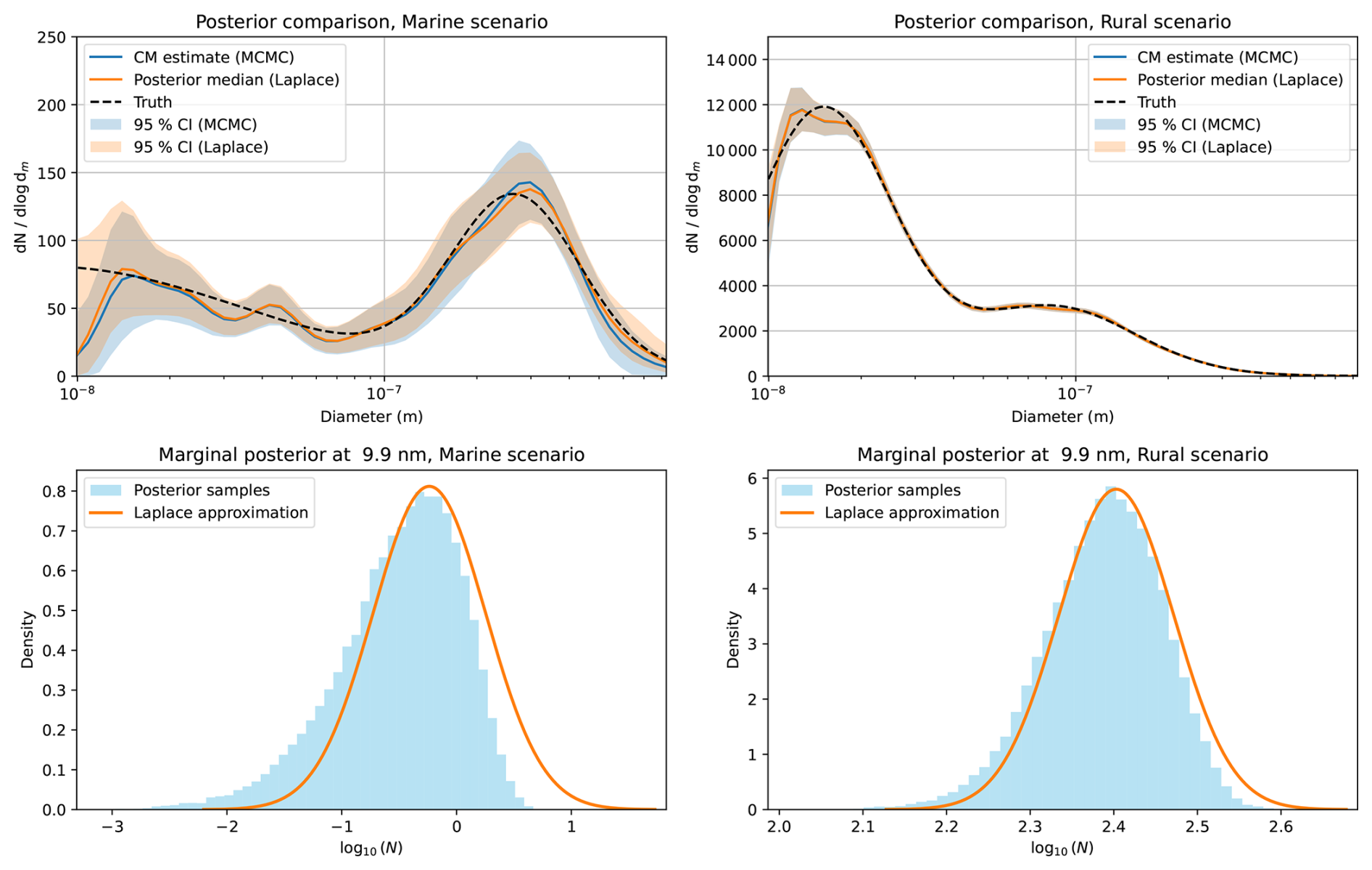
Figure B1 Comparison between the Laplace approximation and the true posterior using sampling.

Figure B1 shows the two scenarios. The top panels display the posterior PSDs and their credible intervals, while the bottom panels show representative 1D marginals in the x-space. In the “Marine” scenario, credible intervals from the Laplace approximation are noticeably inflated at the smallest and largest particle diameters compared to the MCMC posterior. This is shown most clearly in the marginal posterior plot, where the left-skewedness of the true posterior and the symmetry of the Laplace approximation are evident. In contrast, such inflation is not present in the “Rural” scenario, nor in the particle range (20–500 nm) where the DMPS is most sensitive. In all cases, the modes of both the Laplace approximation and the true posterior coincide.

These differences can be explained by the exponential mapping N=10^x in the likelihood. In cases where the relative uncertainty is high (low concentrations, regions of low instrument sensitivity), the likelihood becomes weakly informative and nearly flat for decreasing x, but steep for increasing x. This induces left-skewness in the posterior. At higher concentrations the likelihood dominates and the posterior is nearly Gaussian.

Since the errors from the Laplace approximation show only in low-concentration cases near the extremes of the measurement range, and even then remain negligible near the posterior mode, we conclude that the Laplace approximation is an acceptable trade-off between posterior quality and computational efficiency for our purposes. Nevertheless, MPSS-UQ provides an implementation of a preconditioned adaptive random-walk Metropolis sampler (Andrieu and Thoms, 2008), if full inference is required.