Including the triple isotopic composition of dissolved oxygen in the ocean into the iLOVECLIM model (version 1.1.7): development and evaluation

Contributing around half of the oxygen produced on Earth, marine photosynthetic production is one of the main mechanisms for carbon fixation, with a central role in the oxygen cycle. The triple isotopic composition of atmospheric oxygen (¹⁷Δ), measured in ice cores, provides a global integrator of past biospheric oxygen fluxes, which can also provide indirect constraints on associated carbon-cycle processes. However, deconvolving the signal of ¹⁷Δ requires one to isolate the contribution of oceanic biosphere productivity (¹⁷Δ_ocean) from those of the terrestrial biosphere (¹⁷Δ_terr) and the stratosphere (¹⁷Δ_strato). Here, we present the first implementation of ¹⁷Δ_ocean in the intermediate-complexity climate model iLOVECLIM. The three main processes controlling ¹⁷Δ_ocean, i.e. photosynthesis, respiration, and air–sea gas exchange, are explicitly represented and evaluated under preindustrial conditions. Model results show overall good agreement with available measurements, particularly in the Pacific Ocean. In contrast, systematic overestimation is found in the Southern Ocean. At fixed stations, seasonality is reproduced but with underestimated amplitude. These discrepancies mainly reflect challenges in representing remineralization and oxygen minimum zones, and highlight opportunities to refine the representation of primary productivity and vertical mixing. Overall, this new implementation provides the first coupled model framework for simulating ¹⁷Δ_ocean, both as a diagnostic of biogeochemical processes and as a tool for reconstructing past changes in marine productivity. Extending the implementation to the terrestrial biosphere will further allow reconstruction of the past global biosphere and direct comparison with ¹⁷Δ records from ice cores.

1 Introduction

The triple isotopic composition of molecular oxygen (O₂), preserved in polar ice cores, is a tracer of the past global biosphere productivity (Luz et al., 1999). The triple isotopic composition of tropospheric O₂ reflects two major sources: the global biosphere and the stratosphere. Biogenic O₂ inherits isotopic composition of the source water and is fractionated in mass-dependent manner during biological and hydrological cycling. Conversely, in the stratosphere, O₂ becomes depleted in heavy isotopes in a mass-independent way during ozone-oxygen cycle and isotopic exchange with CO₂ (e.g., Thiemens et al., 1991; Yung et al., 1991; Marcus, 2013). The triple isotopic composition is commonly reported in capital-delta notation (¹⁷Δ) defined as follows (Miller, 2002):

$$\begin{array}{}\text{(1)}& {}^{\mathrm{17}}\mathrm{\Delta }=\left[\ln \left(\mathrm{1}+{\displaystyle \frac{{\mathit{\delta }}^{\mathrm{17}}\mathrm{O}}{\mathrm{1000}}}\right)-\mathit{\lambda }\times \ln \left(\mathrm{1}+{\displaystyle \frac{{\mathit{\delta }}^{\mathrm{18}}\mathrm{O}}{\mathrm{1000}}}\right)\right]\times \mathrm{1}\mathrm{000}\mathrm{000}\end{array}$$

where δ^*O is calculated according to the isotopic ratio of sample (^*R) and of the isotopic standard (^*R_std): δ^*O = ${(}^{*}R{/}^{*}{R}_{\text{std}}-\mathrm{1})\times \mathrm{1000}$, * indicating 17 or 18. The isotopic standard of choice is air O₂ (Luz and Barkan, 2005). Isotopic ratio ^*R (${}^{*}=\mathrm{17}$ or 18) is computed as the abundance ratio of the heavy oxygen isotope (¹⁷O or ¹⁸O) relative to the most abundant oxygen isotope (¹⁶O). Since it is biological processes that generate mass-dependent fractionation, the δ¹⁷O anomaly is established in relation to the triple-isotope slope, i.e. λ=0.518 (Luz and Barkan, 2005). By definition, ¹⁷Δ represents the ¹⁷O anomaly from the mass-dependent fractionation, and is only weakly altered by mass-dependent fractionation in the biosphere and hydrosphere, while remaining sensitive to mass-independent fractionation signals. As a consequence, modern air is depleted in ¹⁷Δ relative to seawater (VSMOW), reflecting stratospheric influx with depleted ¹⁷Δ of O₂. As variations in ¹⁷Δ are very small, it is expressed in ppm (1 ppm=0.001 ‰) relative to air.

Beyond its clear advantage of integrating the global (i.e., terrestrial and marine) biosphere signal, ¹⁷Δ has the potential to constrain contributions from terrestrial and marine biosphere, relying on slightly different isotopic signatures (e.g., Bender et al., 1994; Luz et al., 1999; Luz and Barkan, 2000; Blunier et al., 2002; Landais et al., 2007). To do so, biological processes and associated isotopic effects need to be implemented in a three-dimensional Earth System Model (ESM) to assess the ¹⁷Δ of O₂ produced in the terrestrial (¹⁷Δ_terr) and marine biosphere (¹⁷Δ_ocean). Previous studies have employed isotope-enabled dynamic global vegetation models or ESM to evaluate ¹⁷Δ_terr under past climate boundary conditions, such as during the Last Glacial Maximum (e.g., Landais et al., 2007; Reutenauer et al., 2015; Extier, 2019).

To better quantify the oceanic contribution to the ¹⁷Δ and to understand the underlying processes, various ocean-focused models have been developed, ranging from simple box models to complex ocean circulation models, to simulate and better understand the distribution of dissolved O₂, δ¹⁸O–O₂, and ¹⁷Δ_ocean. A variety of one-dimensional models have been constructed for specific purposes, including: estimating respiratory fractionation factors using a vertical advection model in the deep sea (Kroopnick and Craig, 1976); identifying the factors regulating the δ¹⁸O–O₂ in deep waters (Bender, 1990; Wurgaft et al., 2022); representing ¹⁷Δ_ocean under a stable steady-state (Luz and Barkan, 2000, 2005; Reuer et al., 2007); and evaluating the impact of physical processes on ¹⁷Δ_ocean (Hendricks et al., 2005; Nicholson et al., 2012; Musan et al., 2023). Two-dimensional isopycnal models have been used to represent δ¹⁸O–O₂ in the mesopelagic ocean (Levine et al., 2009), or to understand the distribution of δ¹⁸O–O₂ and ¹⁷Δ_ocean data (Li et al., 2022). Productivity-based models, such as the Vertically Generalized Productivity Model (VGPM; Behrenfeld and Falkowski, 1997) and the Carbon based Productivity Model (CbPM; Westberry et al., 2008), have also been used to estimate ¹⁷Δ_ocean (Juranek and Quay, 2010; Munro et al., 2013). In order to obtain a more detailed and complex representation, the oxygen isotopes and ¹⁷Δ_ocean have been implemented in a global ocean model: the ocean ecosystem and biogeochemistry component of the Community Earth System Model, version 1.1.1 (Nicholson et al., 2014; Palevsky et al., 2016). However, ¹⁷Δ_ocean is not yet implemented in a fully coupled ESM.

All these studies have greatly improved our understanding of these tracers. Both δ¹⁸O–O₂ and ¹⁷Δ_ocean are governed by three main processes: photosynthesis, respiration and exchange at the ocean–atmosphere interface (Hendricks et al., 2004). These studies also highlighted several potential biases affecting the interpretation of ¹⁷Δ_ocean, such as the effect of ocean circulation and the physical processes, or the uncertainties in fractionation coefficients. In order to understand all the processes affecting the triple isotopic composition of dissolved oceanic oxygen, we propose to integrate this tracer into the iLOVECLIM intermediate complexity coupled climate model. This study is divided in three parts: (1) development and verification, (2) evaluation of the model seasonality, (3) evaluation of the minimum oxygen zone representation.

2 Methods

2.1 Oxygen isotopes systematics in the ocean

The calculation of ¹⁷Δ_ocean relies on the isotopic composition of dissolved oxygen (³²O₂, ³³O₂, ³⁴O₂), which is controlled by three main processes: photosynthesis, respiration, and air–sea gas exchange. Consequently, all these processes must be considered to accurately represent the ¹⁷Δ_ocean (Fig. 1 – Green part).

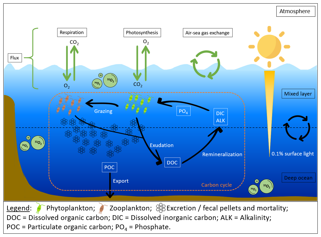
Figure 1 Schematic of the ¹⁷Δ_ocean in iLOVECLIM. The orange part determines the carbon cycle. The green section identifies the processes required to implement ¹⁷Δ_ocean.

2.1.1 Photosynthesis

Photosynthesis is the primary source of molecular oxygen in the ocean. During this process, the isotopic composition of the O₂ produced can be expressed by partitioning Gross Primary Productivity of Oxygen (GPPO₂) among ³²O₂, ³³O₂, ³⁴O₂:

$$\begin{array}{}\text{(2)}& {\displaystyle }\begin{array}{rl}& {}^{*}{\mathrm{O}}_{\mathrm{2}}\text{produced}={}^{*}{\mathit{\alpha }}_{\text{photosynthesis}}\times {}^{*}{R}_{\text{SMOW}}\\ & \times {\displaystyle \frac{{\text{GPPO}}_{\mathrm{2}}}{\mathrm{1}+{}^{\mathrm{17}}{R}_{\text{SMOW}}+{}^{\mathrm{18}}{R}_{\text{SMOW}}}}\end{array}\text{(3)}& {\displaystyle }{}^{\mathrm{32}}{\mathrm{O}}_{\mathrm{2}}\text{ produced}={\mathrm{GPPO}}_{\mathrm{2}}-{}^{\mathrm{33}}{\mathrm{O}}_{\mathrm{2}}\text{ produced}-{}^{\mathrm{34}}{\mathrm{O}}_{\mathrm{2}}\text{ produced}\end{array}$$

where ^*R_SMOW denotes the standard isotopic ratio, either ${}^{\mathrm{17}}\mathrm{O}{/}^{\mathrm{16}}\mathrm{O}$ (for ³³O₂) or ${}^{\mathrm{18}}\mathrm{O}{/}^{\mathrm{16}}\mathrm{O}$ (for ³⁴O₂), based on the Standard Mean Ocean Water (SMOW) reference. α_{photosynthesis} is the isotopic fractionation factor during photosynthesis. The denominator accounts for the total isotopic composition of molecular oxygen (¹⁶O, ¹⁷O, and ¹⁸O). It normalizes the gross primary productivity of oxygen flux, effectively converting GPPO₂ into its ³²O₂-equivalent. This normalization is required because isotopic ratios are conventionally defined relative to ¹⁶O. To ensure conservation of total oxygen productivity, the ³²O₂ produced is calculated as the residual.

2.1.2 Respiration

The oxygen produced by photosynthesis is consumed by the respiration of autotrophic and heterotrophic organisms. Respiration consumes oxygen with a preferential use of light isotopes, generating a mass-dependent fractionation. The ${}^{\mathrm{17}}\mathrm{O}{/}^{\mathrm{16}}\mathrm{O}$ fractionation factor (¹⁷α_respiration) is calculated from ${}^{\mathrm{18}}\mathrm{O}{/}^{\mathrm{16}}\mathrm{O}$ fractionation factor (¹⁸α_respiration) and the triple isotope fractionation exponent (${}^{\mathrm{17}/\mathrm{18}}\mathit{\theta }$), as follows:

$$\begin{array}{}\text{(4)}& {}^{\mathrm{17}}{\mathit{\alpha }}_{\text{respiration}}={(}^{\mathrm{18}}{\mathit{\alpha }}_{\text{respiration}}{)}^{{}^{\mathrm{17}/\mathrm{18}}\mathit{\theta }}.\end{array}$$

Using the fractionation factors, the respiratory consumption of ³³O₂ and ³⁴O₂ is computed assuming mass-dependent isotope effects. The respiratory consumption of ³²O₂ is calculated by ensuring isotopic consistency without altering the total oxygen flows in the system:

$$\begin{array}{}\text{(5)}& {\displaystyle }& {\displaystyle }{}^{*}{\mathrm{O}}_{\mathrm{2}}\text{ respired}={}^{*}{\mathit{\alpha }}_{\text{respiration}}\times {}^{*}{R}_{{\mathrm{O}}_{\mathrm{2}}}\times {\displaystyle \frac{\text{Respiration}}{\mathrm{1}+{}^{\mathrm{17}}{R}_{{\mathrm{O}}_{\mathrm{2}}}+{}^{\mathrm{18}}{R}_{{\mathrm{O}}_{\mathrm{2}}}}}\text{(6)}& {\displaystyle }& {\displaystyle }{}^{\mathrm{32}}{\mathrm{O}}_{\mathrm{2}}\text{ respired}=\text{Respiration}-{}^{\mathrm{33}}{\mathrm{O}}_{\mathrm{2}}\text{ respired}-{}^{\mathrm{34}}{\mathrm{O}}_{\mathrm{2}}\text{ respired}\end{array}$$

where ${}^{*}{R}_{{\mathrm{O}}_{\mathrm{2}}}$ is the fraction of ${}^{*}\mathrm{O}/{}^{\mathrm{16}}\mathrm{O}$ present in the environment. * corresponds to 17 or 18, according to the isotope calculation.

2.1.3 Air–sea gas exchange

To complete the oxygen cycle, exchanges at the air–sea interface must be considered. The net air–sea fluxes of total O₂ is calculated following Nicholson et al. (2012). The negative sign represents that the O₂ molecules are transferred from high to low partial pressure:

$$\begin{array}{}\text{(7)}& F_{\text{net}}=-k_{{\mathrm{O}}_{\mathrm{2}}}({\mathrm{O}}_{\text{surf}}-{\mathrm{O}}_{\text{eq}})\times (\mathrm{1}-f_{\text{ice}})\end{array}$$

with gas piston velocity for oxygen ($k_{\mathrm{O}{}_{\mathrm{2}}}$), concentration of dissolved O₂ at the surface layer (O_surf), saturated concentration of dissolved O₂ (O_eq), and ice cover fraction (f_ice).

The gas exchange flux of heavy isotopologues is calculated by incorporating both equilibrium (^*α_eq) and kinetic isotopic fractionation (^*α_k) as follow:

$$\begin{array}{}\text{(8)}& \begin{array}{rl}{}^{*}F=& {\displaystyle }{-}^{*}{\mathit{\alpha }}_{\text{k}}\cdot k_{{\mathrm{O}}_{\mathrm{2}}}\times \left({{}^{*}\mathrm{O}}_{\text{surf}}{-}^{*}{\mathit{\alpha }}_{\text{eq}}{\cdot }^{*}{R}_{\text{air}}{\displaystyle \frac{{\mathrm{O}}_{\text{eq}}}{\mathrm{1}{+}^{\mathrm{17}}{R}_{\text{air}}+{}^{\mathrm{18}}{R}_{\text{air}}}}\right)\\ {\displaystyle }& {\displaystyle }(\mathrm{1}-f_{\text{ice}})\end{array}\end{array}$$

with ^*R_air is the isotopic ratio of the atmosphere (constant). ${{}^{*}\mathrm{O}}_{\text{surf}}$ is the oxygen isotope concentration in the surface layer. The flux of ³²O₂ is then calculated as a residual to preserve the total oxygen flux.

2.2 iLOVECLIM model

2.2.1 Presentation

Developed from version 1.2 of the LOVECLIM model (Goosse et al., 2010), the iLOVECLIM model is a three-dimensional climate model of intermediate complexity. It is based on fluid mechanics equations and operates on a realistic geographical grid. The simplification of the atmospheric physics enables a relatively fast calculation time with 700–1000 years per day. iLOVECLIM is undergoing continuous developments integrating various climate tracers, in order to improve the representation of climate processes on different time scales. The model retains the main components of LOVECLIM – atmosphere, ocean and vegetation – as described in Goosse et al. (2010); Roche et al. (2007). Below, we briefly describe only the components essential for representing ¹⁷Δ_ocean: the atmosphere, the ocean, and the ocean carbon cycle (Fig. 1).

The atmospheric component, called ECBilt, is represented by a quasi-geostrophic approach with a T21 spectral grid (resolution of 5.6° in latitude and longitude). The atmosphere is subdivided into three vertical levels, with the mid-point of each layer at 800, 500 and 200 hPa (Opsteegh et al., 1998). Humidity is calculated only in the lowest level and is representative of the total humidity content of the atmosphere. Temperature is calculated for two intermediate levels at 650 and 350 hPa. This component represents the entire water cycle (evaporation, precipitation and condensation).

The ocean general circulation component, known as CLIO, is based on the Navier–Stokes equations. Coupled thermodynamically with sea ice (Goosse and Fichefet, 1999; Goosse et al., 2010), this model has a 3°×3° horizontal resolution, a vertical discretization of 20 levels and a free surface that makes it possible to take into account the freshwater input from melting glaciers. Surface temperature and salinity are calculated once a day.

Essential for representing the biological marine ecosystem, the iLOVECLIM model integrates the carbon cycle in the ocean (Bouttes et al., 2015) based on the equations in Six and Maier-Reimer (1996). This simplified model incorporates a single species of phytoplankton, a single species of zooplankton and a single nutrient, phosphate. Nitrate is derived from phosphate in proportion to Redfield ratios, while iron is not represented in the model. Tracers are transported through the ocean by an diffusion–advection scheme. Following a fitted exponential curve, the remineralization profile is reduced at the surface and accentuated in the deep ocean (Bouttes et al., 2015).

In this study, the iLOVECLIM model is run under pre-industrial climate boundary conditions, until prognostic variables in the deep ocean reach equilibrium (3000 years). For these simulations, the following boundary conditions are prescribed: atmospheric CO₂ concentration is fixed at 280 ppm, CH₄ at 760 ppb and N₂O at 270 ppb (Loulergue et al., 2008; Schilt et al., 2010; Bereiter et al., 2015). The solar constant is maintained at 1365 W m⁻² throughout the simulation, and the orbital configuration is set according to Berger (1978). Topography, ice sheets and ocean-continent configuration are prescribed according to current observations. The prescribed boundary conditions are consistent with the PMIP standard for pre-industrial (PI) experiments. Model outputs are reported as the annual average of the variable for each pixel, computed over the last 100 years of the simulation.

2.2.2 Implementation of dissolved oxygen

To simulate ¹⁷Δ_ocean, three tracers corresponding to the bulk abundances of ³²O₂, ³³O₂ and ³⁴O₂ are incorporated into iLOVECLIM through the previously described processes (Fig. 1, Sect. 2.1). The ³³O₂ and ³⁴O₂ tracers correspond to the bulk abundances of the singly substituted isotopologues (i.e., ¹⁶O¹⁷O+¹⁷O¹⁶O and ¹⁶O¹⁸O+¹⁸O¹⁶O, respectively), without explicitly distinguishing between the two symmetry-equivalent molecular arrangements. The three oxygen isotopologues are prognostic tracers whose concentrations are updated at each model time step. Biological O₂ production and consumption, through photosynthesis and respiration, are derived from the marine carbon-cycle model implemented in iLOVECLIM. The production and consumption rates in carbon units are converted into O₂ units using the corresponding Redfield stoichiometric ratios. In contrast, air–sea O₂ exchange is calculated independently from the air–sea CO₂ flux, using O₂-specific formulations (Eq. 8).

The carbon and oxygen cycles are interconnected by biogeochemical processes of photosynthesis and respiration, which involve exchanges between carbon dioxide (CO₂) and oxygen (O₂). Through these processes, a dynamic balance is maintained within the biosphere. The total oxygen concentration in the photic zone is thus calculated as the net result of carbon-related biological processes that either produce or consume oxygen. This oxygen balance is called Net Community Production (NCP), and it is defined by the following equation:

$$\begin{array}{}\text{(9)}& \text{NCP}=\text{PP}-(P_{\text{remin}}+Z_{\text{remin}})-\text{DOC}-\text{DOCs}\end{array}$$

where PP is phytoplankton production and corresponds to phytoplankton growth in the current version of iLOVECLIM. Here, PP is assumed to represent net primary production (NPP). P_remin and Z_remin are the fractions of phytoplankton and zooplankton that are remineralized. DOC is dissolved organic carbon. DOCs is the slowly degradable fraction of DOC. Among these terms, only PP results in net oxygen production.

Although NCP represents the net oxygen balance, isotopic calculations require an explicit separation of gross primary productivity of oxygen and total respiration. Since GPPO₂ and autotrophic respiration are not explicitly simulated by the ecosystem model, we assume that autotrophic respiration is equal to PP, corresponding to a GPP/PP ratio of 2. GPPO₂ is therefore defined as twice the total phytoplankton production after conversion into oxygen units using the Redfield ratio:

$$\begin{array}{}\text{(10)}& {\text{GPPO}}_{\mathrm{2}}=\mathrm{2}\times \text{PP}.\end{array}$$

Here, the factor of 2 represents the assumed GPP/PP ratio and not the overall conversion between carbon-based PP and GPPO₂. When combined with the carbon-to-oxygen conversion using the Redfield ratio ($\mathrm{138}/\mathrm{106}\simeq \mathrm{1.30}$), this formulation results in an overall conversion factor of approximately 2.6 between the carbon-based phytoplankton production simulated by the model and GPPO₂. This factor is close to the ratio between PP (measured by the ¹⁴C method) and GPPO₂, which is 2.7 according to Marra (2002). However, observational estimates range from approximately 1.8 to 4.5 across the ocean (Juranek and Quay, 2013). The use of a spatially constant ratio therefore remains a simplification and may lead to regional over- or underestimation of GPPO₂ and respiration.

Since we cannot distinguish between the autotrophic and heterotrophic respiration in iLOVECLIM, we defined the respiration in a way that conserves the original oxygen budget. As a result, the total respiration of organisms in the mixed layer is defined as:

$$\begin{array}{}\text{(11)}& \text{Respiration}={\text{GPPO}}_{\mathrm{2}}-\text{NCP}.\end{array}$$

While photosynthesis ceases below the photic zone, oxygen consumption can continue down to several kilometers depth, as long as organic matter is available. Respiration is particularly intense in the mesopelagic zone (200–1000 m), where sinking organic matter is actively remineralized. Below this zone, respiration and other oxygen-consuming processes gradually decline with depth. Thus, in the model, these subsurface oxygen consumption processes are represented as:

$$\begin{array}{}\text{(12)}& \text{Remineralization}=-\text{DOC}-\text{DOCs}-\text{POC}\end{array}$$

where POC the Particulate Organic Carbon. All terms expressed in carbon units are converted to oxygen units using the Redfield ratio. The remineralization term is negative, as it represents a net consumption of oxygen. Oxygen isotopologues are calculated using the remineralization flux as the consumption term (Sect. 2.1.2).

In the model, net air–sea fluxes are calculated using a piston velocity parameterized as a quadratic function of wind speed squared (Wanninkhof, 1992), with the oxygen Schmidt number taken from Keeling et al. (1998). The equilibrium saturated oxygen concentration is determined from surface temperature and salinity. Furthermore, isotopic fractionation factors associated with oxygen isotope fractionation are prescribed as constants. For air–sea gas exchange, the equilibrium fractionation factor for ¹⁸O (¹⁸α_eq) is taken from Benson and Krause (1980, 1984), the kinetic fractionation factor (¹⁸α_k=0.9972) from Knox et al. (1992), and the corresponding ¹⁷O fractionation factors (¹⁷α_eq and ¹⁷α_k) from Nicholson et al. (2012). Photosynthesis is implemented without isotopic fractionation (α_{photosynthesis}=1). Respiration applies an ${}^{\mathrm{18}}\mathrm{O}{/}^{\mathrm{16}}\mathrm{O}$ fractionation factor equal to 0.980, with a ${}^{\mathrm{17}/\mathrm{18}}\mathit{\theta }$ of 0.518 (Nicholson et al., 2012, 2014). These values can vary depending on environmental conditions, as observed in different studies and experimental measurements (Table 1). To approach the equilibrium values, it should also be noted that the model is initialized to reproduce a ¹⁷Δ_ocean of 41.5 ppm and a δ¹⁸O–O₂ of 0.151 ‰. To do this, total dissolved oxygen is set to exactly 250 µmol kg⁻¹ and respective isotopic concentrations of ³²O₂ at 249.392 µmol kg⁻¹, ³³O₂ at 0.0959 µmol kg⁻¹ and ³⁴O₂ at 0.5121 µmol kg⁻¹.

Table 1 Respiratory fractionation factors and theta values for ¹⁷O and ¹⁸O oxygen isotopologues.

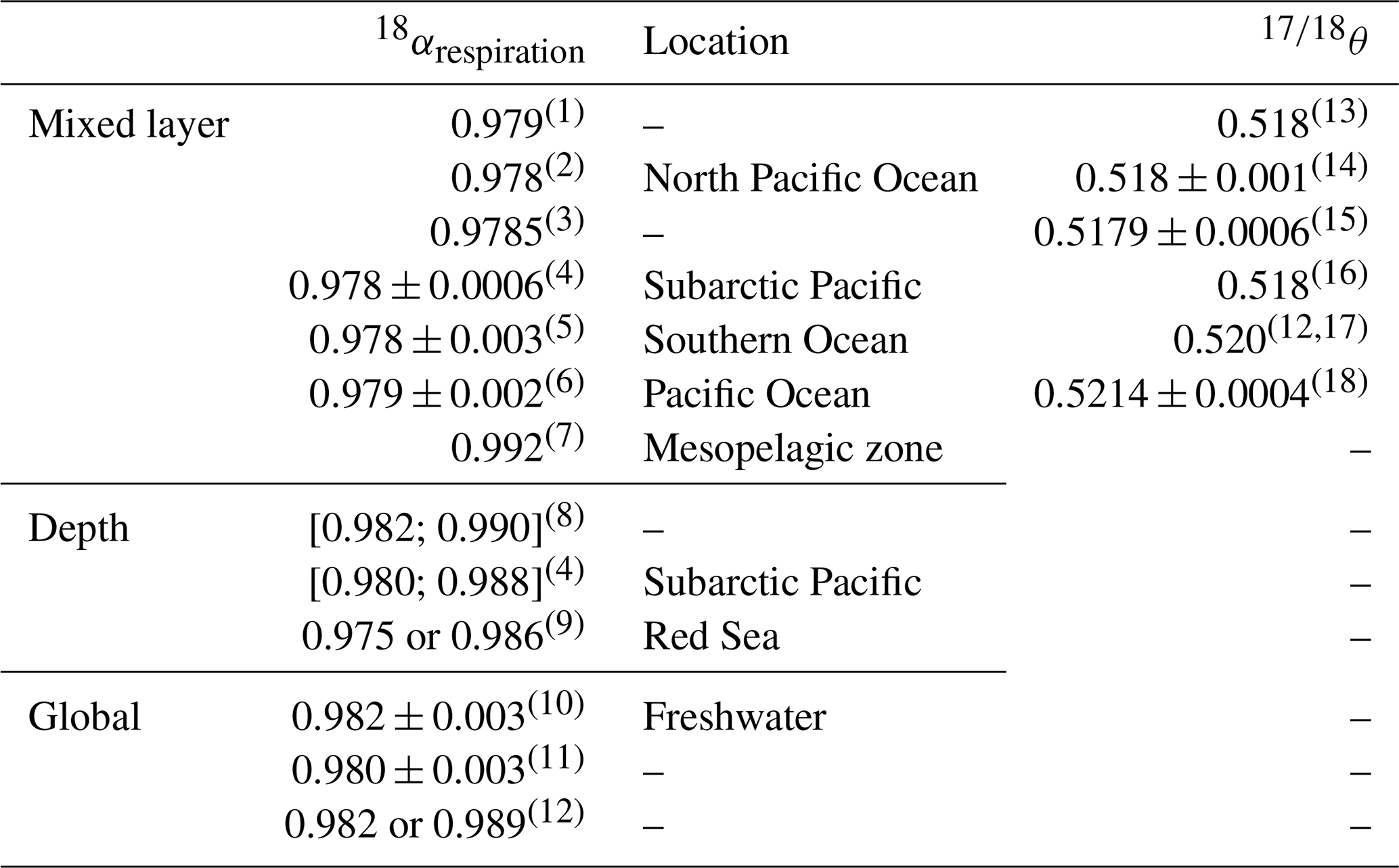
Note: Values reported as average ± uncertainty correspond to the average value together with the associated uncertainty reported in the original study. Values reported as ranges represent the full interval of values reported in the literature. ¹⁸α_respiration and ${}^{\mathrm{17}/\mathrm{18}}\mathit{\theta }$ are independent parameters; not all studies report both. References: (1) Kroopnick (1975); (2) Bender and Grande (1987); (3) Guy et al. (1993); (4) Quay et al. (1993); (5) Hendricks et al. (2004); (6) Hendricks et al. (2005); (7) Levine et al. (2009); (8) Bender (1990); (9) Wurgaft et al. (2022); (10) Quay et al. (1995); (11) Kiddon et al. (1993); (12) Li et al. (2022); (13) Angert et al. (2003); (14) Helman et al. (2005); (15) Luz and Barkan (2005); (16) Juranek and Quay (2013); (17) Ash et al. (2020); (18) Sutherland et al. (2022).

2.3 Observational data

To validate the implementation of the ¹⁷Δ_ocean, a total of 2482 measurements were compiled (Fig. 2). These data were primarily obtained during oceanographic campaigns, where oxygen concentrations were measured either using sensors mounted on a CTD-rosette or by collecting water samples in bottles. The data were processed by averaging replicate measurements and recording their standard deviation. When it was necessary, ¹⁷Δ_ocean value was recalculated using the logarithmic definition (Eq. 1), with a reference slope (λ) of 0.518.

To validate the modelled distribution of total dissolved oxygen, we used annual climatological data from the World Ocean Atlas 2023 (WOA23), provided at 1°×1° horizontal resolution (Reagan et al., 2023). The dataset includes 32 506 unique locations with vertical profiles of dissolved oxygen at various depth. To produce spatial maps from this large dataset, the data points were interpolated using linear interpolation.

It should be noted that the observational datasets used in this study were collected under modern oceanic conditions and represent measurements at specific locations, depths, seasons, and times; whereas the simulations were performed at equilibrium under pre-industrial forcing. Given these differences in temporal representation and the simplified ocean circulation of iLOVECLIM, a point-by-point agreement between model and observations is not expected. Therefore, the geographical comparison is intended to evaluate the large-scale consistency of the simulated oxygen and isotope distributions. As a complementary assessment, the model–data comparison was also examined in temperature–salinity space to evaluate the potential influence of differences in the representation of water masses (Fig. B1).

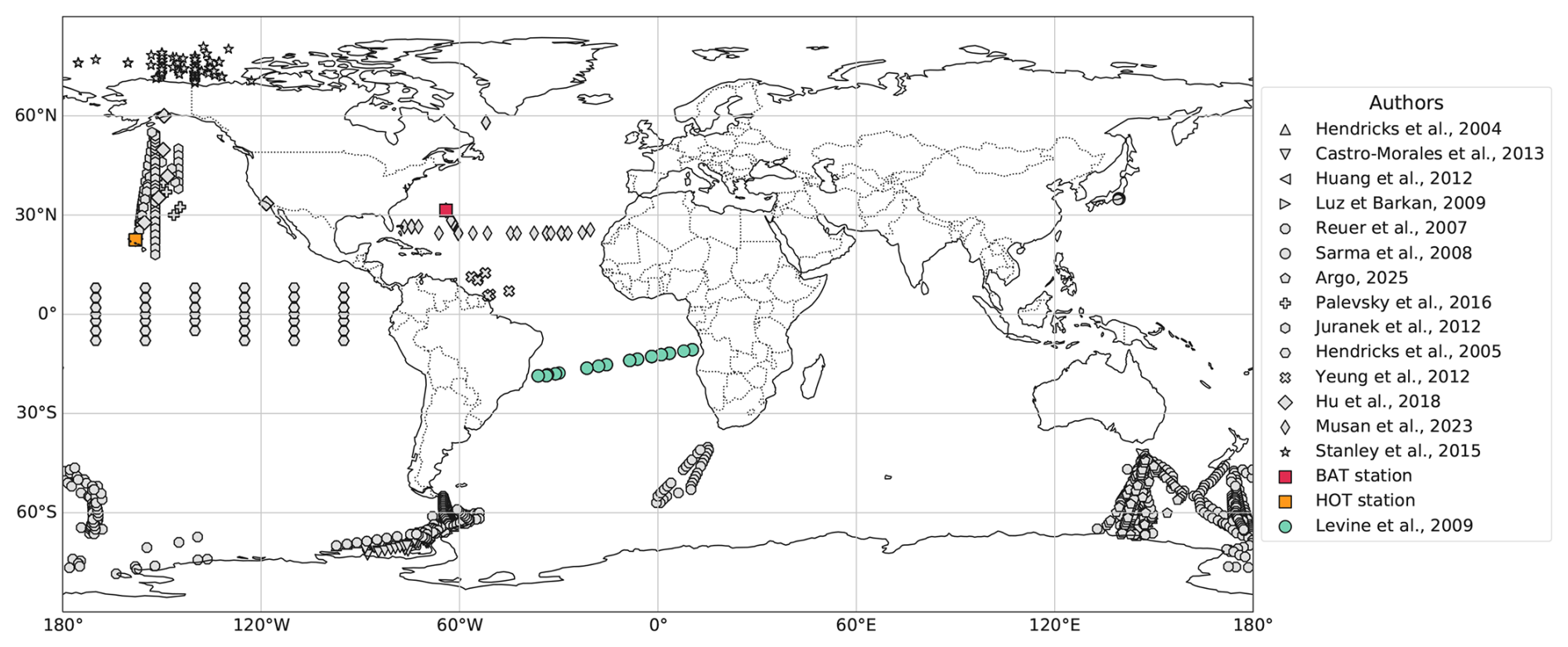
Figure 2 Maps showing measured ¹⁷Δ_ocean data. Symbols correspond to datasets of punctual measurements. Green symbols indicate that only δ¹⁸O–O₂ measurements are available. Squares indicate continuous measurement stations: BAT and HOT.

3 Results

3.1 Total dissolved oxygen

First, we evaluate the modelled distribution of total dissolved oxygen, which serves as the basis for interpreting oxygen isotope tracers. Since total dissolved oxygen reflects both biogeochemical processes and gas exchanges between the air and the sea, a realistic representation is essential to ensure the robustness of the proxy representation. Overall, the distribution of total dissolved oxygen in the photic zone is generally consistent with the interpolated WOA23 data (Fig. 3). In polar regions, the model exhibits a slight depletion of approximatively 30 µmol kg⁻¹ relative to observations. Conversely, some equatorial upwelling areas appear slightly enriched in dissolved oxygen in the model.

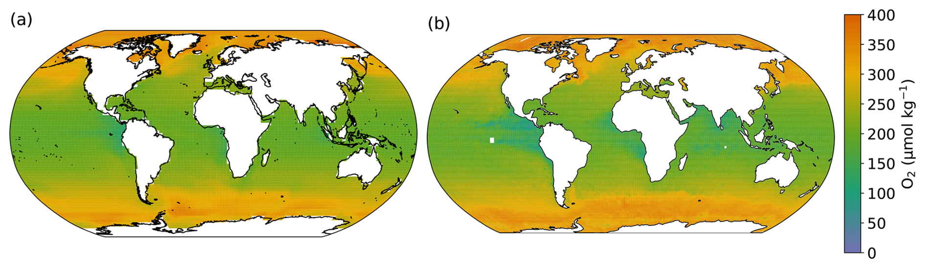
Figure 3 Total dissolved oxygen in the photic layer of the ocean (0–100 m). (a) iLOVECLIM. (b) WOA23 database interpolation (Reagan et al., 2023).

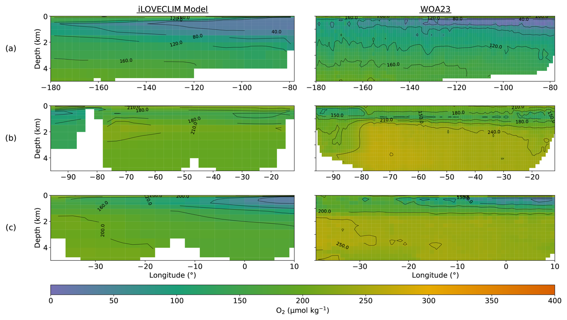
Figure 4 Transects of total dissolved oxygen in the ocean from the iLOVECLIM model (left column) and WOA23 interpolation (right column). Zonal vertical section of meridional mean between (a) 8° S and 5.5° N in Eastern Equatorial Pacific; (b) 24.5 and 28.5° N in the North Atlantic; (c) 10° and 18° S in the tropical South Atlantic Ocean.

Similarly, in the subsurface ocean, the large-scale patterns of dissolved oxygen are generally well captured by the model (Fig. 4). In the Atlantic Ocean, below 2000 m, the model tends to underestimate total dissolved oxygen concentrations (Fig. 4b and c). In both the Pacific and Atlantic Oceans, Oxygen Minimum Zones (OMZ) are overestimated, with simulated low-oxygen regions extending beyond those observed in the data (Fig. 4a and c). In general, the spatial distribution of total dissolved oxygen is reasonably well reproduced by the model, both in the photic zone and at depth, despite some regional discrepancies.

3.2 Gross primary productivity of oxygen

In the iLOVECLIM model, the total phytoplankton production is controlled by three parameters: the maximum daily growth rate, which is influenced by sunlight and temperature; the nutrients availability; and the phytoplankton mass (Six and Maier-Reimer, 1996). Since GPPO₂ is defined as twice the PP in iLOVECLIM, its spatial distribution is governed by these same processes. After evaluating the model's performance in simulating total dissolved oxygen, we next assess GPPO₂, which directly contributes to the isotopic signature observed in surface waters.

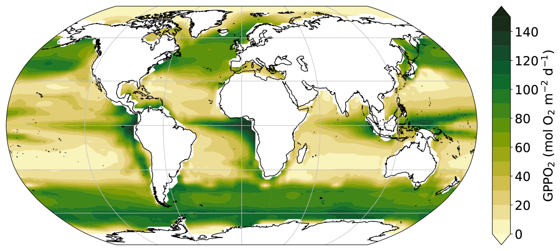
Figure 5 Vertical-integrated GPPO₂ distribution in the photic zone (between 0 and 100 m).

Table 2 GPPO₂ ($\times {\mathrm{10}}^{\mathrm{15}}\mathrm{mol}{\mathrm{O}}_{\mathrm{2}}{\mathrm{yr}}^{-\mathrm{1}}$) in the photic zone of each basin. The simulation was performed under pre-industrial boundary conditions, whereas the ${\text{GPPO}}_{{\mathrm{2}}_{\text{LD}}}$ and ${\text{GPPO}}_{{\mathrm{2}}_{{}^{\mathrm{17}}\mathrm{\Delta }}}$ estimates from Huang et al. (2021) are representative of the modern ocean. ${\text{GPPO}}_{{\mathrm{2}}_{\text{LD}}}$ and ${\text{GPPO}}_{{\mathrm{2}}_{{}^{\mathrm{17}}\mathrm{\Delta }}}$ is derived from a machine-learning reconstruction after correction. ${\text{GPPO}}_{{\mathrm{2}}_{\text{LD}}}$ is based on O₂ evolution during light-dark bottle incubation. ${\text{GPPO}}_{{\mathrm{2}}_{{}^{\mathrm{17}}\mathrm{\Delta }}}$ is based on in situ estimation of ¹⁷Δ_ocean.

Owing to high temperature and maximum solar irradiance, optimum GPPO₂ occurs at the equator, reaching 150 mol ${\mathrm{O}}_{\mathrm{2}}{\mathrm{m}}^{-\mathrm{2}}{\mathrm{d}}^{-\mathrm{1}}$ (Fig. 5). Upwelling regions, where nutrient supply is enhanced, are also areas of elevated GPPO₂. At high latitudes, annual mean GPPO₂ remains elevated because intense spring blooms compensate for low winter production. In contrast, at the center of subtropical gyres, GPPO₂ is low due to the limited availability of nutrients.

The simulation was performed under pre-industrial boundary conditions, whereas the estimates of Huang et al. (2021) are representative of the modern ocean. Therefore, the following comparison focuses on the large-scale patterns and order of magnitude of simulated productivity. Compared with the global GPPO₂ derived from O₂ measurements during incubation and ¹⁷Δ measurements of seawater sample (Huang et al., 2021, Table 2), the GPPO₂ is relatively well represented in the model. Consistent with the two calculation methods presented by Huang et al. (2021), global GPPO₂ is estimated at $\mathrm{9.68}\times {\mathrm{10}}^{\mathrm{15}}\mathrm{mol}{\mathrm{O}}_{\mathrm{2}}{\mathrm{yr}}^{-\mathrm{1}}$ for the pre-industrial simulation (Table 2). However, regional discrepancies are observed: GPPO₂ in the Indian Ocean is underestimated, whereas values in the Arctic and the Southern Ocean are overestimated. The underestimation in the Indian Ocean may reflect limitations in the model's representation of regional processes, such as nutrient supply and monsoon-driven dynamics. Conversely, the overestimation at high latitudes may be due to the absence of iron limitation in the model. Iron is a limiting nutrient for phytoplankton growth, especially in high-nutrient low-chlorophyll regions (HNLC), such as the Southern Ocean and parts of the Pacific Ocean.

3.3 Isotopic tracers: δ¹⁸O–O₂ and ¹⁷Δ_ocean

With both total dissolved oxygen and GPPO₂ reasonably well reproduced by the iLOVECLIM model, we now examine its capacity to simulate oxygen isotope tracers. As mentioned above, the distribution of these tracers is influenced by various processes, including respiration, photosynthesis and air–sea exchange (Hendricks et al., 2004). Hence, isotopic tracers are related to the distribution of total dissolved oxygen: when total dissolved oxygen decreases, isotopic tracers increase (Fig. 6). The choice of isotopic fractionation values also affects tracers distributions. Rayleigh curves were plotted using different fractionation values to illustrate the impact of fractionation during respiration (Figs. 6 and 7). Model-data comparison indicates that isotopic tracers are well captured by iLOVECLIM, although some discrepancies appear for ¹⁷Δ_ocean. These deviations reflect differences in the relative influence of the governing processes.

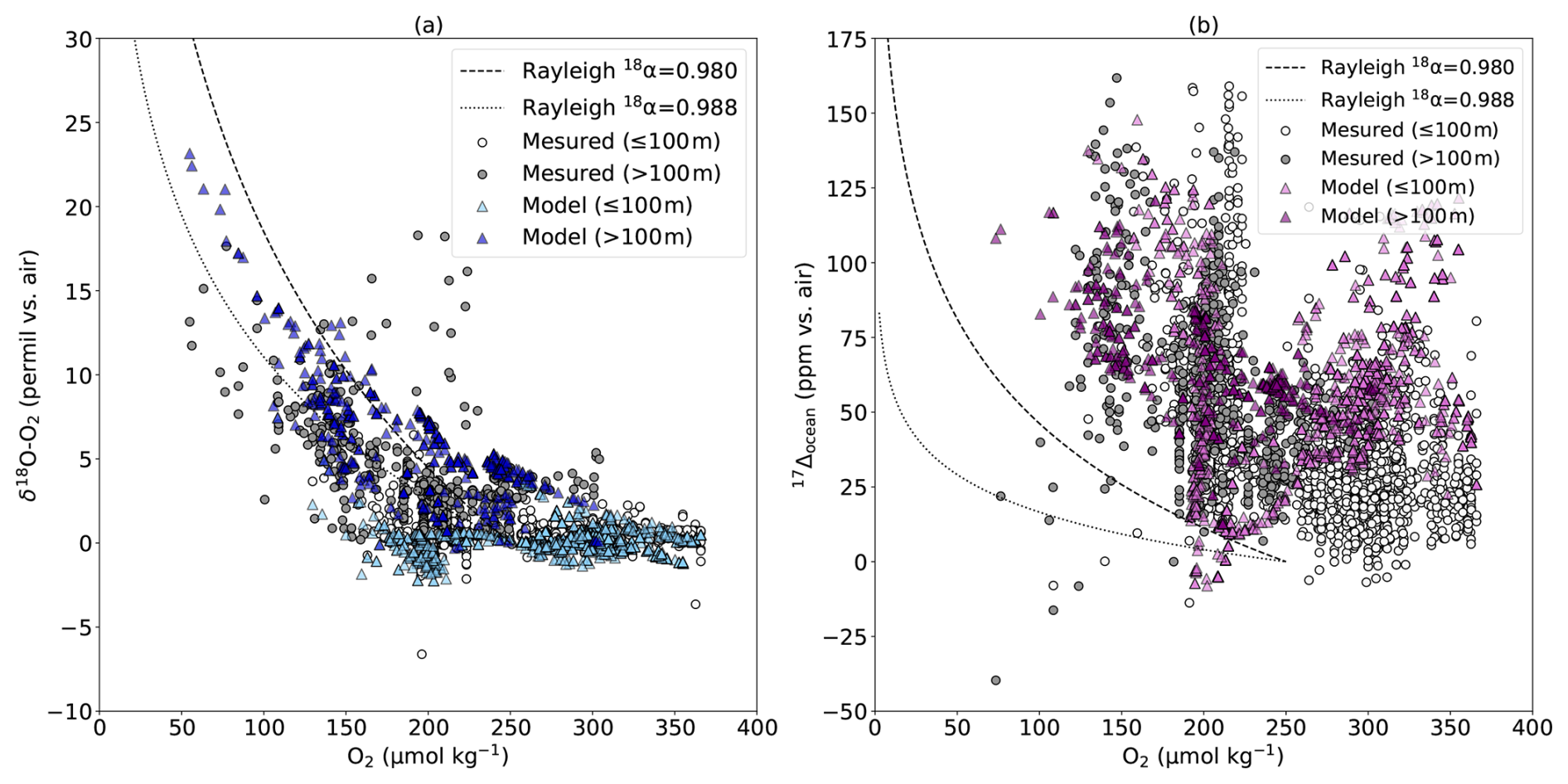
Figure 6 Isotopic tracers according to the total dissolved oxygen concentration. (a) δ¹⁸O–O₂. (b) ¹⁷Δ_ocean. The grey points are the data measurements available (see Fig. 1 for the references). The colored points are the value in the model for the same geographical coordinates as the data. The lines represent Rayleigh slopes with a prescribed alpha.

δ¹⁸O–O₂ is primarily affected by respiration (Figs. 6a and 7a). In surface waters, where O₂ is relatively abundant, the combined processes produce a comparatively stable δ¹⁸O–O₂ signal. In the subsurface waters, where respiration dominates, δ¹⁸O–O₂ follows a Rayleigh-type fractionation trajectory with prescribed fractionation factor. Meanwhile, ¹⁷Δ_ocean reflects the integrated influence of the three processes (Figs. 6b and 7b). When photosynthesis prevails, both ¹⁷Δ_ocean and O₂ concentration increase. In both tracers, air–sea gas exchange exerts a restoring effect, driving δ¹⁸O–O₂ and ¹⁷Δ_ocean toward their respective equilibrium values (Fig. 7).

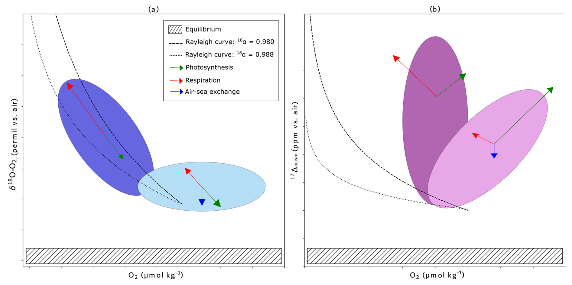
Figure 7 Schematic diagrams of primary factors that control (a) δ¹⁸O–O₂ and (b) ¹⁷Δ_ocean of dissolved O₂. The colored areas show the major distribution of modeled isotopic compositions (Fig. 6). The lighter areas represent the results at the ocean surface, while the darker areas represent the subsurface ocean. Size of arrows qualitatively represent relative contribution of each processes. Axes are not on scale.

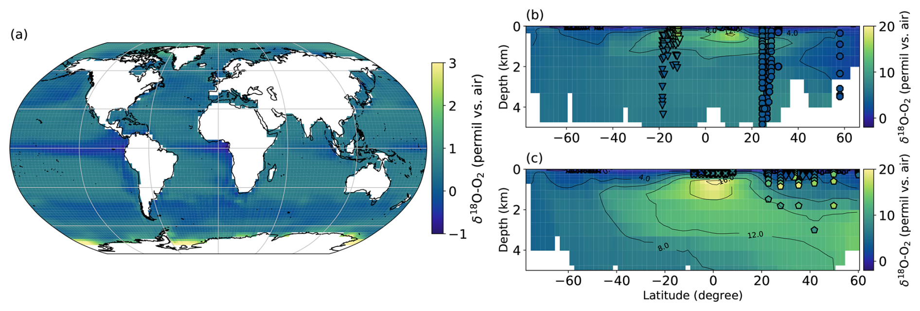
Figure 8 Annual mean distribution of δ¹⁸O–O₂. Points represent measurements of δ¹⁸O–O₂ in the ocean from the literature (see Fig. 1 for the references). (a) Surface. (b) N–S cross-section of the central Atlantic Ocean. In this panel, circles represent data from the BAT station, triangles from Levine et al. (2009), hexagons from Luz and Barkan (2005), another set of hexagons from Yeung et al. (2012), octagons from Musan et al. (2023), and stars from Reuer et al. (2007). (c) N–S cross-section of the central Pacific Ocean. In this panel, hexagons represent data from HOT station, crosses from Hendricks et al. (2005), pentagons from Hu et al. (2018), diamonds from Palevsky et al. (2016), stars from Reuer et al. (2007), and plus signs from Juranek and Quay (2013).

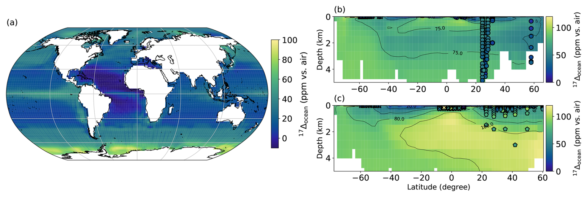
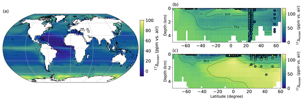
Figure 9 Annual mean distribution of ¹⁷Δ_ocean. Points represent measurements of ¹⁷Δ_ocean in the ocean from the literature (see Fig. 1 for the references). (a) Surface. (b) N–S cross-section of the central Atlantic Ocean. In this panel, circles represent data from the BAT station, hexagons from Luz and Barkan (2005), another set of hexagons from Yeung et al. (2012), octagons from Musan et al. (2023), and stars from Reuer et al. (2007). (c) N–S cross-section of the central Pacific Ocean. In this panel, hexagons represent data from HOT station, crosses from Hendricks et al. (2005), pentagons from Hu et al. (2018), diamonds from Palevsky et al. (2016), stars from Reuer et al. (2007), and plus signs from Juranek and Quay (2013).

The simulated annual mean δ¹⁸O–O₂ distribution reveals clear spatial gradients, both at the surface and at depth (Fig. 8). At the surface, δ¹⁸O–O₂ is about −0.5 ‰ at the equator, while it is about 1 ‰ at the poles (Fig. 8a). Zones of high productivity (equator, upwelling and Southern Ocean) are marked by a depleted δ¹⁸O–O₂, whereas enhanced respiration leads to enrichment. At depth (Fig. 8b and c), δ¹⁸O–O₂ increases relative to the surface, by an average of 7 ‰ in the Atlantic Ocean and 10 ‰ in the Pacific Ocean. The enriched δ¹⁸O–O₂ in the subsurface water masses, in particular around the OMZ, is primarily due to respiration. This is particularly evident within OMZ, where the highest δ¹⁸O–O₂ values are observed, reaching ∼16 ‰ in the Atlantic OMZ and up to ∼22 ‰ in the Pacific OMZ. The stronger enrichment in the North Pacific compared to the Atlantic reflects the older age of water masses, allowing for greater fractionation along the Rayleigh curve. Deep-ocean δ¹⁸O–O₂ values are further modulated by circulation: waters formed in the North Atlantic and around Antarctica begin with relatively high δ¹⁸O–O₂, and their progressive aging along circulation pathways enhances enrichment through cumulative respiration.

The simulated annual mean ¹⁷Δ_ocean distribution reveals different spatial gradients as δ¹⁸O–O₂ (Fig. 9). At the surface, elevated ¹⁷Δ_ocean values indicate regions of high productivity, highlighting the dominant role of GPPO₂. At the Equator, the ¹⁷Δ_ocean is ∼50 ppm, compared with −5 to 20 ppm at the center of the ocean gyres (Fig. 9a). In upwelling regions, nutrient input leads to high phytoplankton productivity, with a ¹⁷Δ_ocean of around 40 ppm. In polar regions, elevated ¹⁷Δ_ocean can be explained by various processes, including the presence of sea ice, or model limitation related to the absence of iron representation. Near Antarctica, values reaching up to 100 ppm are consistent with the seasonal extent of sea ice, which inhibits ocean–atmosphere exchange and leads to the accumulation of ¹⁷Δ_ocean beneath the ice. At the end of the Antarctic winter, the maximum extent of sea ice can reach 55° S latitude, emphasizing the vast area where seasonal air–sea fluxes are blocked. At depth, similarly to δ¹⁸O–O₂, an increase of ¹⁷Δ_ocean values is observed (Fig. 9b and c). This vertical distribution can partly be explained by the sinking of water masses, which transports high values to the deep ocean. Additionally, at depth, signals may reflect both the accumulation of respiration and the presence of old water masses.

To reduce the impact of seasonal variability, the model–data comparison focuses on deep-ocean values, where signals are more stable over time (Figs. 8b and c, 9b and c). For both δ¹⁸O–O₂ and ¹⁷Δ_ocean, the simulated values fall within the observed range in the Pacific and Atlantic basins. However, in the Atlantic Ocean, modeled values tend to be overestimated in the subsurface ocean. For example, at 20° S and 3 km depth, simulated δ¹⁸O–O₂ reach 7 ‰, while observational data indicate a value closer to 3 ‰, corresponding to a relative error of approximatively 133 % (Fig. 8b). At the same location, simulated ¹⁷Δ_ocean at 2 km depth shows a relative error of ∼30 % compared to observations, with discrepancies increasing below 4 km. Several hypotheses could explain this overestimation, such as: excessive surface oxygen production exported to depth via Antarctic Bottom Water (AABW), or an inaccurate representation of the AABW dynamics in the model. The choice of values for ¹⁸α and ${}^{\mathrm{17}/\mathrm{18}}\mathit{\theta }$ during respiration are also factors that may induce an overestimation. In addition, part of the discrepancy may reflect the inherent uncertainties and sampling limitations of the observational datasets. Musan et al. (2023) suggest that observed data in this region may also be partly influenced by Labrador Sea Water, in particular the Iceland-Scotland Overflow Water (ISOW) and Denmark Strait Overflow Water (DSOW) masses. Such an influence could reduce the apparent discrepancy between simulated and observed ¹⁷Δ_ocean values. By contrast, in the model this region is largely dominated by AABW, as illustrated in Fig. 9b.

These results demonstrate that the model provides a robust first-order representation of the δ¹⁸O–O₂ and ¹⁷Δ_ocean distributions. The discussion below addresses the origins of the remaining biases.

4 Discussion

4.1 Seasonal effect

The deep ocean results suggest a slight overestimation of ¹⁷Δ_ocean driven by AABW formation and water mass sinking. At the surface ocean, away from the equator, the distribution of ¹⁷Δ_ocean is additionally modulated by seasonal effects. Therefore, to evaluate its distribution in the photic layer, it is crucial to compare observational data with simulated seasonal ¹⁷Δ_ocean outputs. This is particularly relevant given that most of available observational data are measured from surface water samples collected at specific time, and reflect the state of surface water ecosystem over a few weeks. Year-round observations are only available at research stations (e.g. HOTS, BATS, etc).

For this purpose, monthly modelled ¹⁷Δ_ocean values were extracted within the photic layer (0–100 m) at the exact locations of the available measurements to allow a direct comparison (Fig. 10). In the Pacific Ocean, simulated ¹⁷Δ_ocean values generally fall within the observed range. No clear seasonal pattern emerges from the comparison, although slightly larger deviations are observed for some locations during SON (September–October–November) and DJF (December–January–February). In the Southern Ocean, iLOVECLIM consistently overestimates ¹⁷Δ_ocean, with all simulated points lying above the 1:1 line. Whereas observed values range from 0–80 ppm, the model estimates span from 20–160 ppm. Notably, neither the data nor the simulations exhibit a clear seasonal pattern. Due to the scarcity of measurements in the Atlantic Ocean, a robust assessment of ¹⁷Δ_ocean representation in this basin is not possible.

As mentioned above, several hypotheses may explain the overestimation of ¹⁷Δ_ocean in the Southern Ocean: (1) the absence of iron limitation in the iLOVECLIM model, which favors excessive phytoplankton growth and thus amplifies the photosynthetic ¹⁷Δ_ocean signal; and/or (2) the accumulation of the ¹⁷Δ_ocean under sea-ice. However, the second hypothesis is unlikely to play a major role here, as sea ice cover is minimal during the DJF season. Overall, this overestimation is most likely due to an overrepresentation of primary production in the model. Since PP depends on three key parameters, it seems possible to improve its representation by further refining the model and adjusting the parameters.

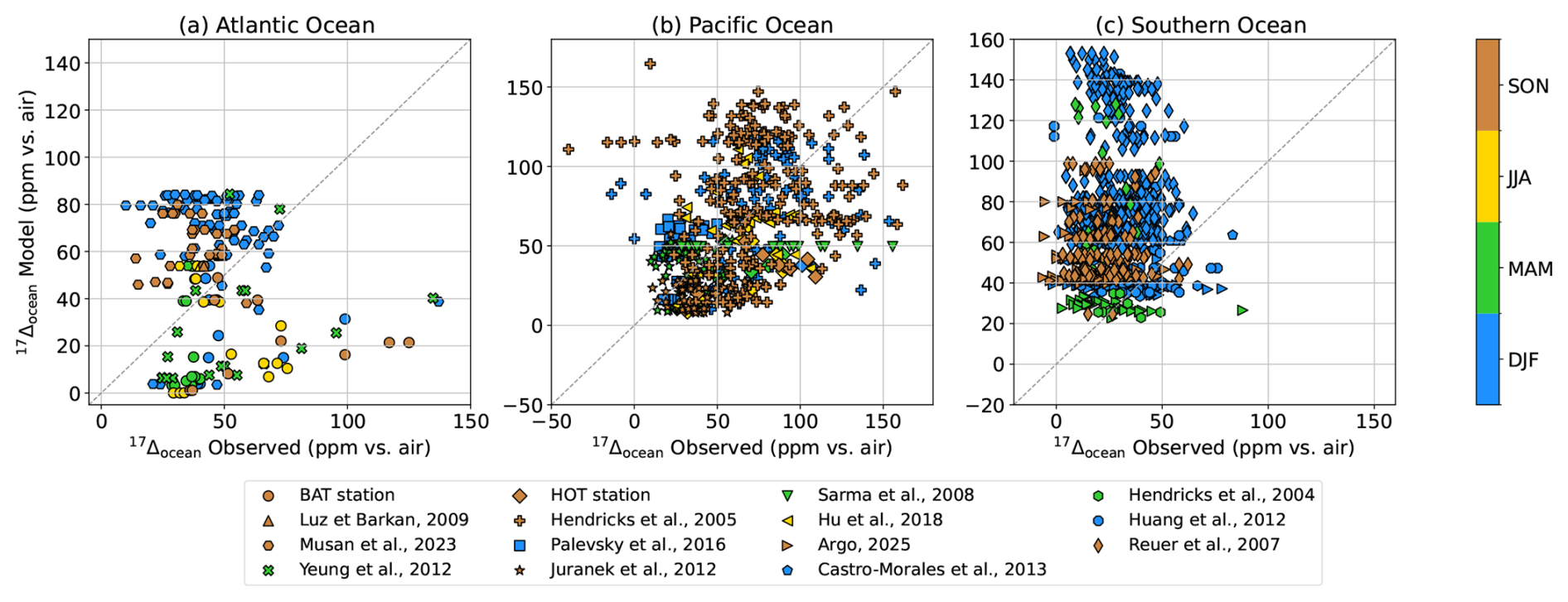
Figure 10 Comparison by basin in the photic zone of simulated ¹⁷Δ_ocean according to measured ¹⁷Δ_ocean. The different markers represent the references. The colors represent the seasons, with: SON = September, October, November; JJA = June, July, August; MAM = March, April, May; DJF = December, January, February. The black dotted line represents a 1:1 straight line.

Year-round measurements at the BATS and HOTS allow for the seasonal assessment of the model's ability to represent ¹⁷Δ_ocean across depth and basin at fixed coordinates. Overall, both measured and simulated ¹⁷Δ_ocean display seasonal variability within the upper photic layer (Fig. 11). At BATS, measured ¹⁷Δ_ocean stabilizes below 250 m, while at HOTS, stabilization occurs around 300 m across all seasons. In contrast, the modelled ¹⁷Δ_ocean stabilizes much shallower, around 100 m, limited by the prescribed photic layer depth. In both observational and simulated profiles, the most pronounced seasonal variation occurs between 50 and 100 m. While the model successfully captures the seasonal trend, it underestimates the amplitude. For instance, during SON, ¹⁷Δ_ocean peaks at 120 ppm in the measurements, but only reaches  45 ppm in the model. Despite this underestimation, the seasonal cycle of ¹⁷Δ_ocean in the photic layer is reasonably well reproduced.

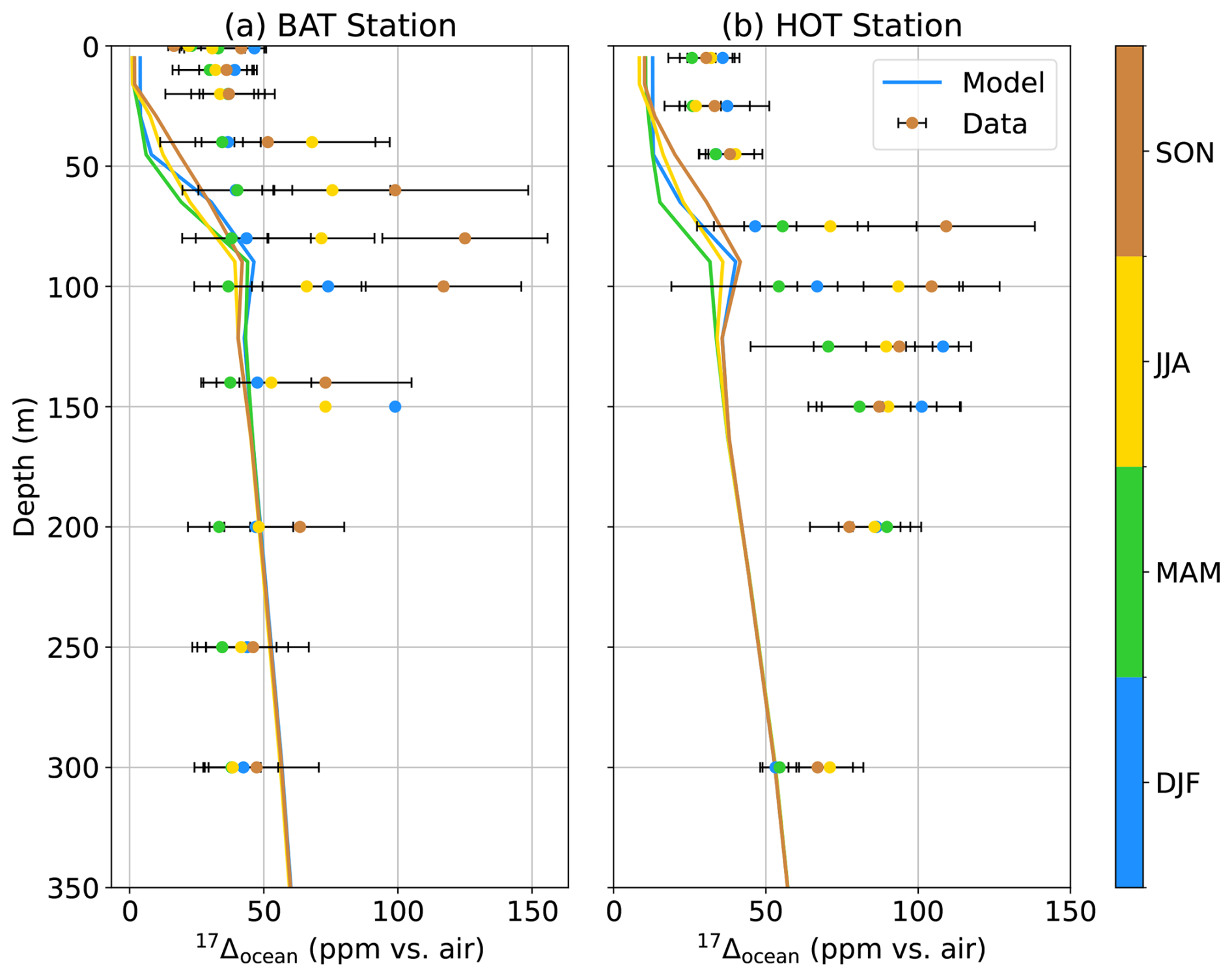
Figure 11 Vertical profile of ¹⁷Δ_ocean according to the seasons, in Bermuda Atlantic Time-series (BAT) and in Hawaii Ocean Time-series (HOT). The lines represent the simulated evolution of ¹⁷Δ_ocean, while the dots represent measured ¹⁷Δ_ocean values with associated error bars. The colors represent the seasons, as described in Fig. 10.

Overall, the model captures the seasonal trend of ¹⁷Δ_ocean reasonably well across different spatial scales, from ocean basins to fixed-point stations. However, it systematically over-estimates absolute ¹⁷Δ_ocean values in the Pacific and Southern Oceans when compared point by point with observations. At station level, although the seasonal phase is reproduced, the amplitude remains underestimated and the vertical structure is too shallow, likely due to limitations in the photic layer depth and primary production representation. Indeed, limited variability in PP can reduce the production of oxygen, leading to an underestimation of ¹⁷Δ_ocean at these stations. Other factors, such as local mixing processes or nutrient limitations, may also contribute, but the insufficient seasonal modulation of biological activity appears to be a primary driver (Appendix A). These discrepancies suggest that while the timing of seasonal variability is well represented, further refinement of the biological and vertical mixing processes in the model is necessary to improve the magnitude and spatial distribution of ¹⁷Δ_ocean. Importantly, the implementation of ¹⁷Δ_ocean revealed this bias, providing a direct diagnostic of the model's ability to reproduce seasonal cycles.

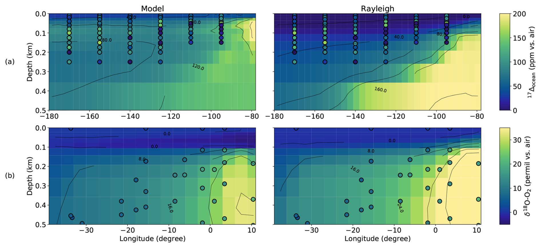
Figure 12 East–west transect of isotopic proxies at depth. The first column “Model” represents the result of the model. The second column “Rayleigh” represents the proxy calculated theoretically according to the Rayleigh slope with α=0.980 (Fig. 6), based on the oxygen present in the model. The dots represent the measured proxy. (a) Zonal vertical section of meridional mean of ¹⁷Δ_ocean between 8° S and 5.5° N in Eastern Equatorial Pacific. (b) Zonal vertical section of meridional mean of δ¹⁸O–O₂ between 10 and 18° S in the tropical South Atlantic Ocean.

4.2 Oxygen minimum zone

Beyond seasonal dynamics, the distribution of total dissolved oxygen is another factor that can indirectly influence ¹⁷Δ_ocean. In iLOVECLIM, oxygen minimum zones tend to expand excessively, leading to unrealistic remineralization rates. To prevent such issues, an ad hoc lower oxygen threshold was introduced in the model. After testing, a minimum total oxygen concentration of 30 µmol kg⁻¹ was established, below which remineralization is halted to ensure numerical stability. However, this constraint also prevents the full development of OMZ. While it avoids unrealistic anoxia, it limits the emergence of strong subsurface oxygen gradients, which in turn may reduce the biogeochemical contrast necessary to simulate realistic isotopic composition around this region.

To further evaluate the representation of ¹⁷Δ_ocean and δ¹⁸O–O₂ in the model, we compare them against the OMZ using both theoretical estimates and available observations (Fig. 12). The theoretical proxy is computed using a Rayleigh fractionation model, which isolates the effect of respiration while neglecting photosynthesis, water mass mixing and air–sea exchange. It provides a useful benchmark to assess the consistency between the simulated oxygen field (Fig. 4) and the expected isotopic gradients, by isolating the influence of remineralization. This comparison serves as a diagnostic of the model's internal consistency.

In the eastern equatorial Pacific, both the model and theoretical calculations show an eastward increase in ¹⁷Δ_ocean, near the American coast (Fig. 12a). However, sparse observational data in this region limit direct validation. The theoretical signal exhibits a more pronounced vertical gradient and higher values toward the east compared to the model. In contrast, the simulated ¹⁷Δ_ocean is further diffuse, potentially due to excessive smoothing of primary production, limited vertical resolution, or inaccurately tuned remineralization rates. Additional contributions may arise from inaccurate isotopic fractionation values during both photosynthesis and respiration, which would directly affect the magnitude and vertical structure of ¹⁷Δ_ocean. For δ¹⁸O–O₂ (Fig. 12b), the model simulates strong enrichment along the eastern boundary, where OMZ are expected (Fig. 4c). However, observed values are lower, suggesting an overestimation of the isotopic signal associated with respiration. This bias may result from excessive remineralization just above the 30 µmol kg⁻¹ threshold in iLOVECLIM, which suppresses anoxia while still allowing intense localized biogeochemical activity. Other potential biases include excessive remineralization rates, overestimation of isotopic fractionation during respiration, or mixing between different water masses. In addition, limited vertical mixing may amplify this signal. While remineralization under low oxygen conditions could occur, the behavior of isotopic fractionation under such conditions remains largely unknown. Diapycnal mixing may also contribute to the observed patterns. As a result, the model produces a truncated OMZ but an exaggerated isotopic response, complicating the interpretation of δ¹⁸O–O₂ in these regions.

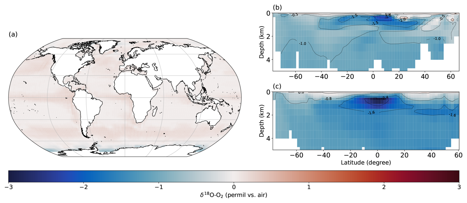
Figure 13 Differences in simulated δ¹⁸O–O₂ between the simulation using the equilibrium and kinetic isotope fractionation factors from Li et al. (2019) and the reference simulation (Exchange–CTRL). (a) Surface ocean. (b) N–S cross-section of the central Atlantic Ocean. (c) N–S cross-section of the central Pacific Ocean.

Overall, this comparison highlights the value of combining isotopic proxies, theoretical simulations, and biogeochemical fields to diagnose internal model limitations. In particular, when the oxygen field reproduces expected structures but the associated isotopic signal does not, this may indicate a decoupling between biological processes and isotopic dynamics.

4.3 Isotope fractionations during air–sea exchange

Air–sea gas exchange is one of the three fundamental processes controlling the isotopic composition of dissolved oxygen. The reference simulation (CTRL) uses the equilibrium and kinetic isotope fractionation factors described in Sect. 2.2.2. To evaluate the sensitivity of the isotopic tracers to recently revised air–sea isotope fractionation factors, we performed an additional simulation, hereafter referred to as the Exchange experiment, using the parameterization of Li et al. (2019). The corresponding fractionation factors are summarized in Table 3. Compared with the CTRL simulation, the equilibrium fractionation factor for ¹⁸O remains unchanged, whereas the kinetic fractionation factor for ¹⁸O and both the equilibrium and kinetic fractionation factors for ¹⁷O are updated.

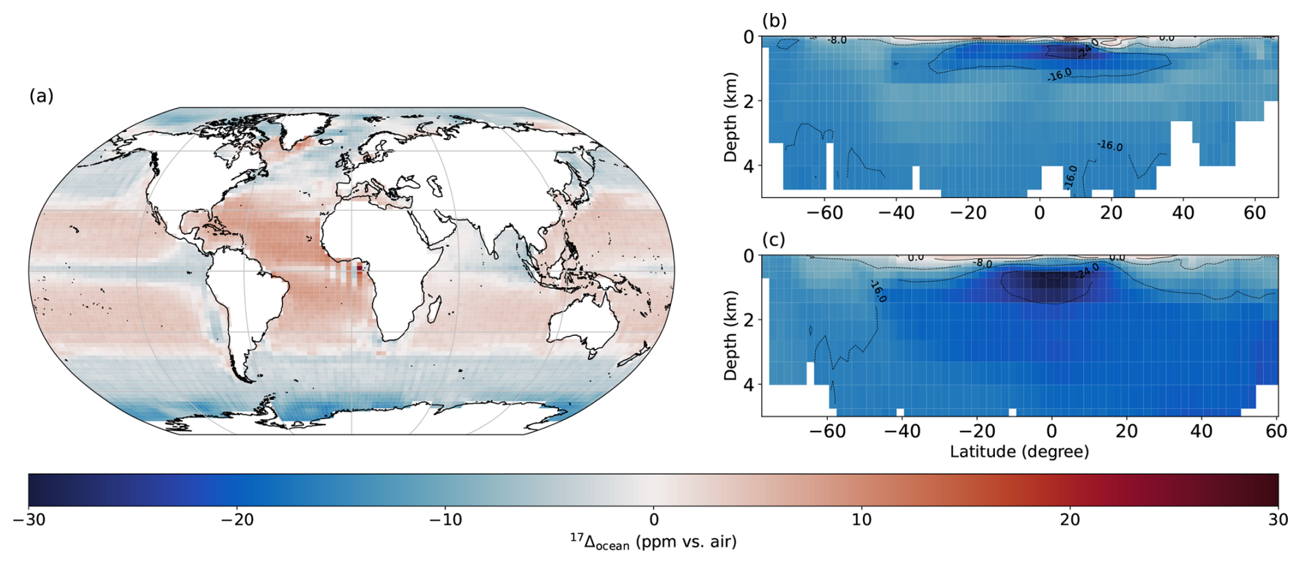
Figure 14 Differences in simulated ¹⁷Δ_ocean between the simulation using the equilibrium and kinetic isotope fractionation factors from Li et al. (2019) and the reference simulation (Exchange–CTRL). (a) Surface ocean. (b) N–S cross-section of the central Atlantic Ocean. (c) N–S cross-section of the central Pacific Ocean.

Figure 13 shows the differences in simulated δ¹⁸O–O₂ between the simulation using the updated air–sea exchange fractionation factors and the reference simulation (Exchange–CTRL). The impact of the revised parameterization on simulated δ¹⁸O–O₂ remains relatively small at the ocean surface (Fig. 13a), with anomalies generally ranging between −0.5 and 0.5 ‰. Surface waters exhibit slightly higher δ¹⁸O–O₂ values in the Exchange simulation, except in the Southern Ocean where lower values are observed. These negative anomalies propagate into the ocean interior, leading to decreases of up to 2.5 ‰ within oxygen minimum zones (Fig. 13b and c).

The impact is more pronounced for ¹⁷Δ_ocean (Fig. 14). At the ocean surface, differences range from approximately −10 to 10 ppm, with depleted values in the mid-to-high latitudes and equatorial regions, while enhanced values occur in the subtropical gyres (Fig. 14a). This spatial pattern highlights the regional influence of air–sea gas exchange on the isotopic composition of dissolved oxygen, especially in the regions of relatively weak biological productivity (e.g., subtropical gyres) or intense air–sea gas exchange (e.g., Southern Ocean). In the ocean interior, ¹⁷Δ_ocean in the Exchange simulation decreases by up to approximately 16 ppm, with maximum differences reaching −24 ppm within oxygen minimum zones (Fig. 14b and c). These pronounced anomalies indicate that changes in the isotopic signature acquired during air–sea gas exchange are subsequently transported into the ocean interior, where they amplify the differences between the two simulations.

Table 3 Equilibrium and kinetic isotope fractionation factors that differ between the reference simulation (CTRL) and the simulation using the updated air–sea gas-exchange parameterization of Li et al. (2019) (Exchange).

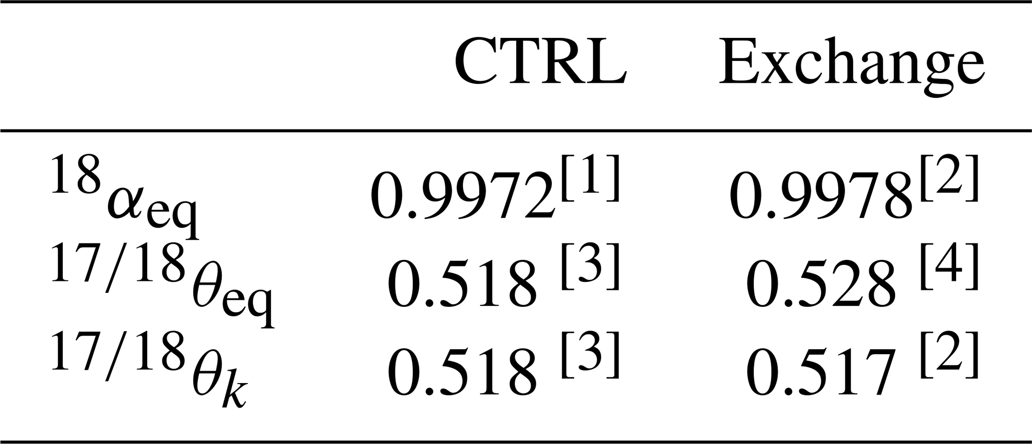
Note: [1] Knox et al. (1992); [2] Li et al. (2019), [3] Nicholson et al. (2012), [4] Reuer et al. (2007); Palevsky et al. (2016).

These changes are consistent with the experimental results of Li et al. (2019), confirming that the revised air–sea gas-exchange isotope fractionation factors exert a non-negligible influence on the isotopic composition of dissolved O₂. Despite these regional differences, the overall agreement between simulations and observations changes only marginally. The coefficient of determination remains unchanged for δ¹⁸O–O₂ (R²=0.70 for both simulations), while it increases slightly for ¹⁷Δ_ocean, from R²=0.02 in CTRL to R²=0.03 in the Exchange simulation. These relatively low coefficients mainly reflect the comparison of climatological model fields with sparse observations collected over different seasons, years, and spatial scales, rather than a point-by-point evaluation. Nevertheless, the updated coefficients noticeably improves the simulated isotope fields in oxygen minimum zones and in the Southern Ocean. Within oxygen minimum zones, the revised fractionation factors reduce δ¹⁸O–O₂ by up to 2.5 ‰ and ¹⁷Δ_ocean by up to 24 ppm, thereby reducing the model bias relative to the limited observations available in these regions (Fig. 12). Similar improvements are found in the Southern Ocean, although significant discrepancies remain. These results suggest that the revised air–sea gas-exchange fractionation factors improve the regional distribution of the simulated isotope fields but cannot, by themselves, explain the remaining Southern Ocean model–data discrepancies. Additional physical and biogeochemical processes are therefore likely to contribute to the persistent biases.

5 Conclusions

In this study, we implemented the triple isotopic composition of dissolved oxygen into the iLOVECLIM model, providing the first representation of ¹⁷Δ_ocean in a 3D Earth System Model of intermediate complexity. Validation against available observations shows that total dissolved oxygen, GPPO₂ and δ¹⁸O–O₂ are reasonably well represented, enabling the model to simulate coherent ¹⁷Δ_ocean distributions. The model successfully captures the timing of seasonal variability in oxygen isotopes, demonstrating its ability to reproduce large-scale temporal dynamics. However, a key limitation lies in the representation of oxygen minimum zones, which remains constrained by the imposed oxygen threshold. To improve the spatial distribution and magnitude of ¹⁷Δ_ocean, further refinement of primary production schemes and vertical mixing processes is needed, particularly in the Southern Ocean, where adopting the updated air–sea gas-exchange isotope fractionation factors of Li et al. (2019) improves the simulated isotope fields but does not fully resolve the remaining model–data discrepancies, indicating that additional physical and biogeochemical processes are likely involved. In addition, uncertainties associated with isotopic fractionation factors and atmospheric boundary conditions may contribute to the remaining discrepancies between simulations and observations. Future sensitivity analyses will help quantify their influence on simulated δ¹⁸O–O₂ and ¹⁷Δ_ocean, and distinguish parameter uncertainty from model structural limitations. These findings emphasize the possibility of constantly improving the reproduction of this proxy. They also highlight the importance of understanding the underlying physical and biogeochemical processes affecting the ¹⁷Δ. This new implementation also opens the way for future applications of iLOVECLIM to reconstruct past variations in ocean productivity. The future integration of terrestrial ¹⁷Δ_terr into iLOVECLIM will also enable the reconstruction of the past global biosphere and the comparison of these reconstructions with ¹⁷Δ measurements from air bubbles in ice cores.

Appendix A: Seasonal phytoplankton productivity (PP)

In the main text, we compared the results of ¹⁷Δ_ocean at the BAT and HOT stations. One possible explanation for the limited variability observed is the relatively stable phytoplankton productivity (PP) in these regions. To explore this further, we compared the model outputs with available PP observations at the BAT (Johnson et al., 2025) and HOT (White et al., 2025) stations.

Figure A1 shows that PP exhibits only limited seasonal variability at both sites. This limited variability likely reflects the relatively stable environmental conditions in these subtropical regions. PP is calculated according to three parameters, which are: nutrient availability, temperature and light function, and finally phytoplankton mass. Refining the parameterization of these drivers could help improve the representation of seasonal PP, and consequently, the seasonal behavior of ¹⁷Δ_ocean.

It is worth noting that the model used here is of intermediate complexity. While not all biogeochemical processes are explicitly represented, it provides a robust annual mean representation of ¹⁷Δ_ocean, consistent with the scope and objectives of this study.

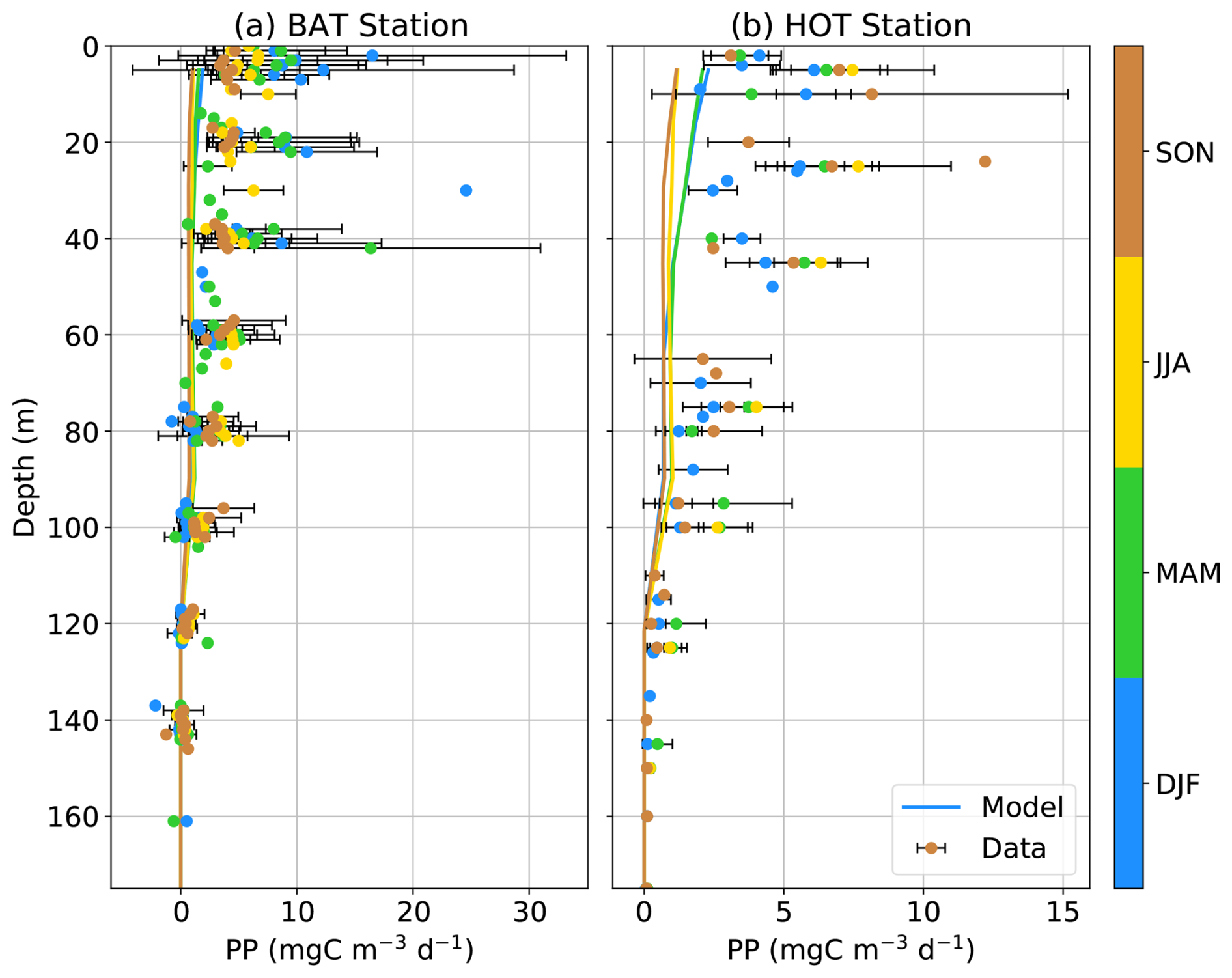
Figure A1 Vertical profile of phytoplankton productivity according to the seasons, in Bermuda Atlantic Time-series (BAT) and in Hawaii Ocean Time-series (HOT). The lines represent the simulated evolution of PP, while the dots represent measured PP values with associated error bars. The colors represent the seasons.

Appendix B: Model–data comparison in temperature–salinity space

To complement the geographical model–data comparison, the distribution of ¹⁷Δ_ocean was also examined in temperature–salinity (T–S) space (Fig. B1). Model values correspond to the grid cells, depths, and seasons associated with each observation. The observations span a broader range of hydrographic conditions than the corresponding simulated waters, particularly toward lower salinities, whereas the model occupies a narrower T–S space. This indicates that some local model–data discrepancies may be associated with differences in the representation of water masses in iLOVECLIM. However, for waters occupying comparable temperature and salinity ranges, the positive ¹⁷Δ_ocean bias previously identified in the Southern Ocean remains clearly visible, with simulated values generally higher than observed ones. This suggests that the Southern Ocean bias cannot be explained solely by the comparison of dissimilar water masses and may reflect a more systematic model behaviour in this region.

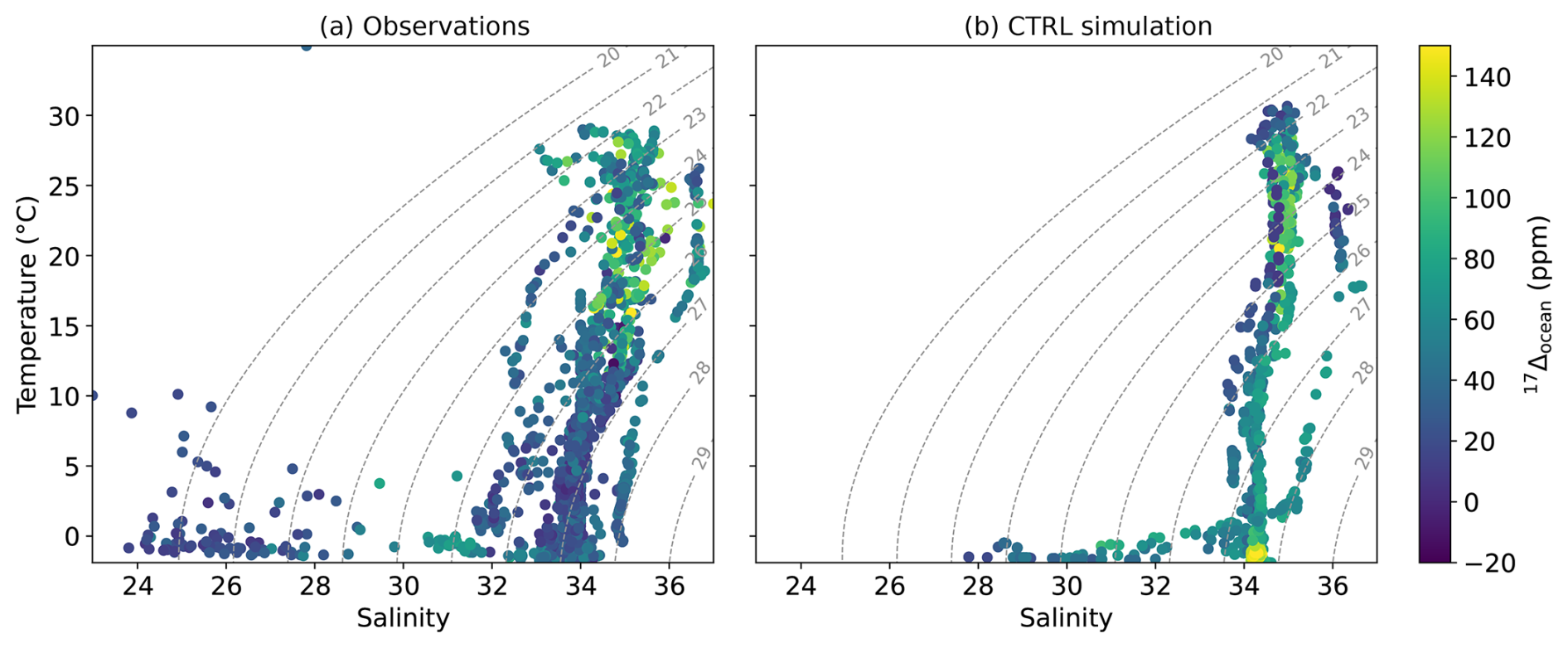
Figure B1 Temperature–salinity (T–S) diagrams for (a) observations and (b) the CTRL simulation, colored according to ¹⁷Δ_ocean (ppm). Model values correspond to the grid cells, depths, and seasons associated with the observations. Dashed lines indicate seawater density contours.