AstroComb(v.1.0): non-linear, multi-channel, probabilistic cyclostratigraphic analysis

We present a new algorithm for constructing floating astronomical timescales with explicit uncertainty estimates from sedimentary sequences. The method integrates probabilistic spectral analysis with inverse geochronological modelling, applied to ultra-high-resolution, multi-proxy datasets such as core scanning X-Ray Fluorescence (XRF) elemental records. Our framework does not smooth data or impose layer-to-layer dependency, allowing sedimentation rates to vary abruptly at short stratigraphic length scales. By detecting and statistically constraining Milankovitch cycles preserved in stratigraphic signals, the algorithm seeks a floating age-depth model that reconstructs geological time and can be anchored to deliver absolute age assignment, when astronomical tie points and/or radioisotopic ages are available. The resulting timescales enable precise, uncertainty-bounded timing of biostratigraphic zones, geochemical events, and depositional cycles. This approach advances astrochronology by combining cycle detection with formal stratigraphic modelling, while preserving fine-scale depositional variability, offering a reproducible and statistically rigorous framework for dating deep-time records.

1 Introduction

Astronomical forcing of Earth’s climate system produces quasi-periodic variations in sedimentary records that can be used to construct geological timescales, reconstruct daylength, Earth system evolution, and investigate the long-term dynamics of the Solar System (Hinnov, 2013, and references therein). Astrochronology has therefore become a central component of modern geochronology and is now widely used in calibration of the Geological Timescale (Laskar, 2020), reconstruction of past climate variability (Hays et al., 1976; Pälike et al., 2006), and studies of Earth–Moon distance and Solar System evolution (Ma et al., 2017; Meyers and Malinverno, 2018; Zhou et al., 2024). Improvements in astrochronological methodologies therefore have implications extending beyond stratigraphy, influencing multiple areas of geoscience and planetary science.

The fundamental challenge in astrochronology is that sedimentary records preserve orbital forcing only indirectly. Variability in sedimentation rates, changes in depositional environments, diagenetic overprinting, and nonlinear sedimentary responses distort the astronomical signals. Furthermore, in deep-time studies beyond approximately 50–60 Ma, theoretical orbital solutions become unreliable due to the chaotic evolution of the Solar System (Laskar et al., 2004, 2011). As a result, astrochronology requires inverse methods that infer sedimentation histories and test consistency with orbital forcing.

Over the past two decades, several classes of inverse astrochronologic methods have been developed to address this problem. Early methods, such as Average Spectral Misfit (ASM) evaluates spectral peaks against astronomical frequencies across sedimentation rates and was later extended to moving-window analysis (eASM; Meyers and Sageman, 2007).

Bayesian spectral methods later formalized this framework by evaluating the power concentrated in astronomical frequencies relative to a noise model formulated as a likelihood function (Malinverno et al., 2010; Peng et al., 2023; Trayler et al., 2024). Parallel developments introduced time-domain approaches including TimeOpt (Meyers, 2015) and time-variant sinusoidal modeling (Sinnesael et al., 2016; ACE v.1) along with extensions (Sinnesael et al., 2018; Meyers and Malinverno, 2018; Malinverno and Meyers, 2024; Hoang et al., 2025), while correlation-based methods such as COCO and eCOCO evaluated agreement between measured and theoretical power spectra (Li et al., 2018). More recently, AstroGeoFit has introduced a unified, uncertainty-aware framework that jointly optimizes sedimentation rates and enables rigorous error estimation in age–depth models (Hoang et al., 2025). Together these methods have substantially advanced quantitative astrochronology and uncertainty assessment.

Sedimentation is an inherently unsteady and discrete process, influenced by short-lived hiatuses and implicit erosion that result in nonlinear time-depth relationships across all time scales (Kemp and Sexton, 2014). Mass accumulation is affected by deposited grains and diagenetic processes inside the sediments, including cementation, authigenic mineral formation and recrystallization. Milankovitch insolation forcing may influence deposited grains as well as diagenetic products. The sediment composition is also affected by other cyclic processes, for example biogeochemical resonances and local autogenic deposition processes (Zhao et al., 2023; Paola, 2016; Munnecke et al., 2001). These processes may introduce abrupt local variations in mass accumulation rates that are difficult to capture using approaches that assume smoothly varying sedimentation. In the following, we use “sedimentation rates” to refer broadly to all mass-accumulation rates in a sedimentary drill core.

We introduce AstroComb – a probabilistic framework for combining multi-channel geochemical records to identify signatures of astronomical periodicities. The goal is to construct floating astronomical timescales and to estimate sedimentation rates within stratigraphic sections while explicitly quantifying the associated uncertainties. Conceptually, AstroComb builds on the Bayesian spectral inversion approach of Malinverno et al. (2010) but extends it in several important ways.

First, the method simultaneously incorporates multiple observational channels, allowing information from independent geochemical proxies to constrain sedimentation-rate estimates. Second, the method allows abrupt local variations in sedimentation rate where supported by the data. Third, the framework explicitly quantifies uncertainty by estimating full posterior probability distributions for sedimentation rates at every stratigraphic position. The current version of AstroComb looks for multiple periodic signals with given relative periods for selected astronomical insolation forcings, and is currently not designed to independently validate whether such fit is indeed driven by insolation variations, e.g. by seeing eccentricity-driven amplitude modulations on precession and/or obliquity cycles.

The AstroComb method operates through a sliding-window probabilistic inversion in which observed local spectra are compared with target astronomical frequencies under a range of candidate sedimentation rates. The resulting posterior distributions provide estimates of sedimentation rates, uncertainty, and information content as a function of stratigraphic depth.

We evaluate the performance of AstroComb first by using synthetic datasets designed to test the recovery of abrupt sedimentation-rate changes under substantial noise contamination. Then, we apply AstroComb to ultra-high-resolution X-ray fluorescence (XRF) data from the upper Cambrian Alum Shale Formation of Scandinavia. The Alum Shale represents an ideal test case because of its preservation of orbital-scale cyclicity (Sørensen et al., 2020; Zhao et al., 2022). Using approximately 90 000 measurements spanning ∼ 19 m of stratigraphy, we evaluate whether probabilistic multi-channel analysis can recover orbitally forced signals while recovering variability in sedimentation rates.

2 Theory and Methods

2.1 Overview

The goal of this study is to reconstruct a locally varying sedimentation rate profile with errorbars from multiple geochemical depth series, under the assumption that certain stratigraphic signals (e.g., elemental variability) reflect astronomical forcing. We achieve this by inverting a forward model of signal distortion under varying sedimentation, using a formulation rooted in probabilistic inversion.

This method builds upon the principles of astrochronology, particularly the spectral identification of Milankovitch-band periodicities in sedimentary records, but extends them to allow for instantaneous, non-stationary sedimentation rates. AstroComb performs a sliding-window probabilistic fit of observed geochemical spectra to a predefined target astronomical spectrum, yielding a sedimentation rate for the mid-point in the window that optimally “stretches” or “compresses” the time axis at each position to recover astronomical frequencies. The fit is performed in frequency domain, which allows multi-channel (e.g. multiple elements) that will not be obscured if displaced by a phase-lag.

We begin by formalizing the relationship between sedimentation rate and spectral distortion, then describe the inversion procedure and implementation of AstroComb. Finally, as an example, we discuss its application to the Alum Shale data and compare to previous cyclostratigraphic results (Sørensen et al., 2020).

2.2 Forward Model of Spectral Distortion

Let d(z) be a geochemical depth series (e.g., Al concentrations), where z is stratigraphic depth. If sediment accumulated at a locally constant rate, $r\left(z\right)=\frac{\mathrm{d}z}{\mathrm{d}t}$, then in the time domain, the corresponding series is d_t(t). However, in practice we only observe the signal in the depth domain.

Let k be a frequency in the depth domain (wave number in cycles per mm) and f its time-domain counterpart (cycles per kyr). The transformation between the two is:

$$\begin{array}{}\text{(1)}& k={\displaystyle \frac{f}{r}}\end{array}$$

Thus, a fixed astronomical frequency f will appear in the stratigraphic record as a peak at k, depending on the local sedimentation rate. Variations in r(z) distort the signal, shifting, splitting, or smearing spectral peaks (Schiffelbein and Dorman, 1986; Ripepe and Fischer, 1991; Herbert, 1994; Meyers et al., 2001). Our objective is to recover r(z) such that the observed power spectrum matches that predicted from astronomical forcing (see Fig. 1).

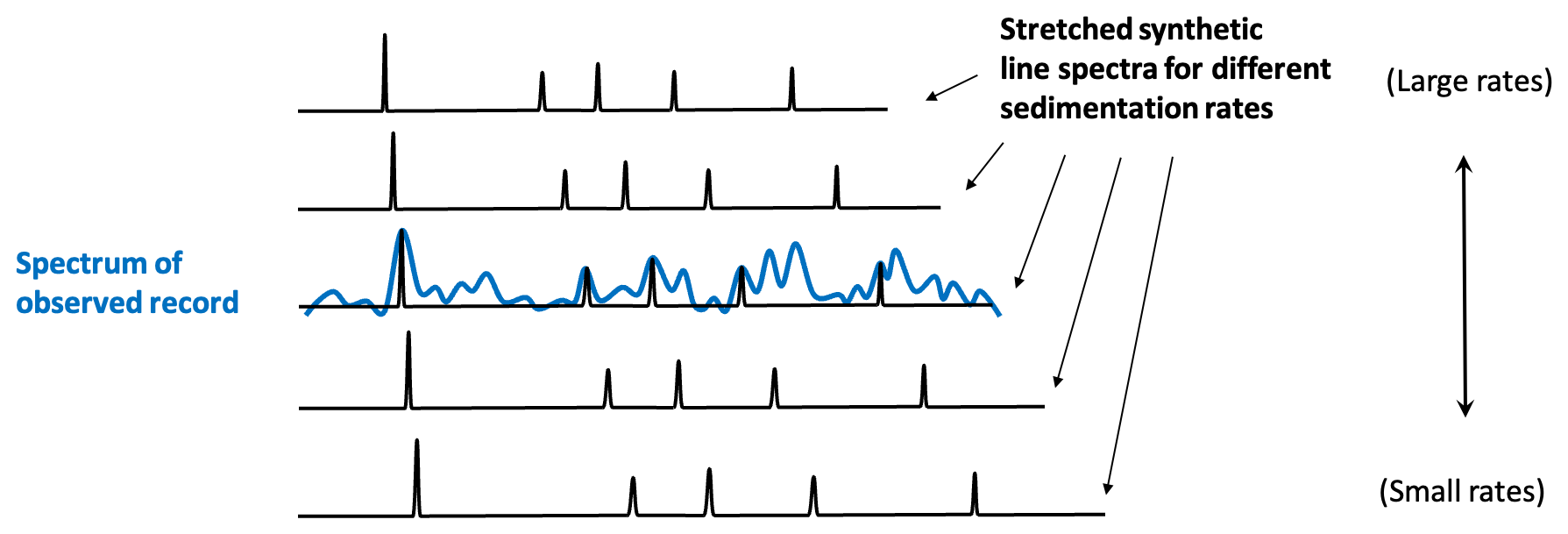
Figure 1 Schematic overview of the likelihood calculation for fitting Milankovitch cycles in elemental profiles. The spectrum of the observed geochemical signal (e.g., Al content) is compared against a theoretical line spectrum, composed of known astronomical frequencies, and stretched according to the sedimentation rate. The likelihood of each assumed sedimentation rate is computed from the probabilities that amplitudes at line locations are significant peaks. This process yields probability distributions of sedimentation rates as a function of depth, and allows an age–depth model consistent with Milankovitch forcing to be computed.

2.3 Computing the Likelihood of a Sedimentation Rate

For a given depth interval (window) centered at z₀, we obtain power spectra D_obs of multiple, observed signals (D_obs is a matrix of spectra with a spectrum of one channel in each column). For each trial sedimentation rate r, we convert the target time-domain frequencies f to expected depth-domain frequencies (wave numbers) $k=f/r$.

In our computation of the likelihood, data uncertainties are indirectly provided by the user as the probability that a peak in the observed spectrum at a given trial wavenumber is a Milankovitch peak. Existing data-fitting-based methods (Meyers and Sageman, 2007; Malinverno et al., 2010; TimeOpt: Meyers, 2015; TimeOptMCMC: Meyers and Malinverno, 2018; AstroGeoFit: Hoang et al., 2025) are purely based on misfits between data (elemental records) and synthetic signals (generated from assumed Milankovitch periods), but AstroComb is instead aimed at simulating the spectral peak identification and data uncertainty evaluation carried out by practitioners analyzing observational data. In traditional misfit calculations you not only need experimental uncertainties, but also the variance of components of the data that are not modeled by the Milankovitch cycles. These components are significant, but not directly available (for example, The TimeOptMCMC algorithm estimates them through a Hierarchical Bayes approach (Meyers and Malinverno, 2018)). However, in our approach we are automatically taking all data uncertainty sources into account, using the practitioner's confidence in identifying spectral peaks.

The most (almost universally adopted) definition of the likelihood would, in our case, read

$$\begin{array}{}\text{(2)}& L\left(\mathbf{m}\right)=p_{\mathrm{n}}({\mathbf{D}}_{\mathrm{obs}}-g(\mathbf{m}\left)\right)\end{array}$$

where p_n is the noise distribution, D_obs is the observed multi-channel data, and g(m) is the forward function mapping the unknown model parameters m into the data. We can see from Eq. (2) that the likelihood depends on m through the function g, so we can define a non-negative function p_d such that

$$\begin{array}{}\text{(3)}& p_{\mathrm{d}}\left(g\right(\mathbf{m}\left)\right)\equiv L\left(\mathbf{m}\right).\end{array}$$

Since g(m) is the “noise-free data”, we can view p_d as the (possibly unnormalized) distribution of the noise-free data, given that we only know the observations D_obs and the data uncertainties p_n (Tarantola, 2005). However, Eq. (3) also shows that a likelihood can be calculated by any procedure that measures the goodness of fit, based on a forward function g and observations D_obs. The underlying uncertainty need not be given in advance through a noise distribution p_n. If the goodness of fit is a priori acceptable for the analyst (e.g., based on experience), p_n can be determined afterwards, if needed. In the following we follow a procedure where we define the likelihood without an initial definition of p_n.

Our likelihood calculation is as follows:

1. As prior information about the data uncertainties, we mimic the 'manual' process of spectral line identification by defining a probability that there is a potential Milankovitch peak at a given wavenumber k in the spectrum. Between user-defined lower and upper bounds a (the lower limit for being identified as a “peak”) and b (the value above which we are sure that we have found a potential peak), the probability increases from a user defined, small positive number p_a at the lower limit to $p_b=\mathrm{1}-p_a$ at the upper limit. Typical values are $a=\langle F\rangle +{\mathit{\sigma }}_F$ and $b=\langle F\rangle +\mathrm{3}{\mathit{\sigma }}_F$, where 〈F〉 is a local mean of the spectrum around the considered wavenumber k, and σ_F is the local standard deviation of the spectrum. In our implementation, 〈F〉 was found as the value of a background spectrum at wavenumber k, where the background was calculated as a smooth function fitted to the power spectrum. We fitted the spectrum with a sum of three decreasing exponentials, but other ways are possible. Our threshold probability p_a is 0.01. The probability function p(x) is chosen from user experience, and in our implementation it was chosen as a smooth, monotonically increasing sigmoid function satisfying

   $$\begin{array}{}\text{(4)}& p\left(a\right)=p_a,p_b\left(b\right)=\mathrm{1}-p_a,\end{array}$$

   with the constraints

   $$\begin{array}{}\text{(5)}& b>a,\mathrm{0}<p_a<\mathrm{0.5},\end{array}$$

   with the form

   $$\begin{array}{}\text{(6)}& p\left(x\right)={\displaystyle \frac{\mathrm{1}}{\mathrm{1}+\exp (-k(x-x_{\mathrm{0}}\left)\right)}}\end{array}$$

   with

   $$\begin{array}{}\text{(7)}& x_{\mathrm{0}}={\displaystyle \frac{a+b}{\mathrm{2}}}.\end{array}$$

2. For each layer (which is Δz=0.2 mm thickness in the Fågeltofta-2 core), we evaluate the likelihood in a grid of sedimentation rates r with typical grid spacing Δr=0.02 mm kyr⁻¹. Each possible choice corresponds to given locations of the Milankovitch cycles in the spectrum, and for each location at k_i with observed spectral amplitude a_i, we evaluate the probability π(k_i, a_i) of having a Milankovic peak at that location. Finally, the likelihood of the considered sedimentation rate r is computed as the product

   $$\begin{array}{}\text{(8)}& L\left(r\right)=\prod _{i=\mathrm{1}}^{I_{\mathrm{M}}}\mathit{\pi }(k_i,a_i),\end{array}$$

   where I_M is the number of Milankovitch cycles considered. For example, when several records of major element concentrations are used in the calculation, the combined likelihood for all records is computed as the product of the individual likelihoods assuming that noise on different channels are independent of each other.

2.4 The Posterior Probabilities of Sedimentation Rates

If prior information about (r, a) is encoded by a probability density ρ(r, a) we can – in a Bayesian formulation – express the complete, probabilistic solution as a posterior probability density

$$\begin{array}{}\text{(9)}& \mathit{\sigma }(r,\mathbf{a})=C\cdot L(r,\mathbf{a})\mathit{\rho }(r,\mathbf{a}).\end{array}$$

where C is a proportionality constant. In the example below, where data from Fågeltofta-2 is analyzed, the prior is uniform and assigns constant values to all sedimentation rates within user-defined boundaries of 1.0 mm kyr⁻¹ $<r<\mathrm{10.0}$ mm kyr⁻¹.

From the marginal sedimentation rate distribution

$$\begin{array}{}\text{(10)}& \mathit{\sigma }\left(r\right)=\int \mathit{\sigma }(r,\mathbf{a})\mathrm{d}\mathbf{a}\end{array}$$

at each stratigraphic position, we can now compute a floating geological time, t, and its uncertainties as a function of depth, z. If the absolute time, t₀, is known at a given depth z₀, and the sedimentation rate in layer n is r_n, the time at z₀+NΔz is

$$\begin{array}{}\text{(11)}& t(z_{\mathrm{0}}+N\mathrm{\Delta }z)=t_{\mathrm{0}}+\mathrm{\Delta }z\sum _{n=\mathrm{1}}^N{\displaystyle \frac{\mathrm{1}}{r_n}}.\end{array}$$

From the posterior probability densities of the sedimentation rates r_n, and hence $\mathrm{\Delta }z/r_n$, we can now calculate the uncertainties of the times, t. From the variances of the distributions of $\mathrm{\Delta }z/r_n$ for all layers n, we can obtain the variance of t(z₀+NΔz) by a simple summation:

$$\begin{array}{}\text{(12)}& \mathrm{Var}\left(t\right(z_{\mathrm{0}}+N\mathrm{\Delta }z\left)\right)=\sum _{n=\mathrm{1}}^N\mathrm{Var}\left({\displaystyle \frac{\mathrm{\Delta }z}{r_n}}\right).\end{array}$$

Working with variances, instead of the full probability distributions for the inverse sedimentation rates, saves computer storage and time when processing large data sets. Furthermore, due to the central limit theorem, the distribution of the sum of random time increments will converge to a Gaussian distribution when the number of layers increases, making the variance an adequate description of the uncertainty.

Finally, we calculate the Kullback-Leibler information measure at each depth z showing how much Milankovitch information is present in the data as a function of depth (Kullback and Leibler, 1951). This is obtained from:

$$\begin{array}{}\text{(13)}& \mathcal{I}=\underset{R}{\int }{\mathit{\sigma }}_z\left(r\right)\ln \left({\displaystyle \frac{{\mathit{\sigma }}_z\left(r\right)}{u\left(r\right)}}\right)\mathrm{d}r\end{array}$$

where σ_z(r) is the calculated probability distribution of r at depth z, R is the range of sedimentation rates, and u(r) is a uniform (constant, and hence non-informative) distribution. Theoretically, the Kullback-Leibler information measures the expected number of yes/no questions needed to update our state of information from what is given by u(r) (here total ignorance) to what is given by σ_z(r) (here, the posterior distribution).

2.5 The AstroComb Algorithm

AstroComb implements the above approach through the following steps:

1. Preprocessing: Detrend and normalise the depth series, optionally re-sample or smooth.

2. Sliding Window: For each depth window (an interval with length, e.g., 2–4 m chosen by the user), compute the local power spectrum.

3. Spectral Inversion: Fit the observed spectrum to the target astronomical model. (The user defines the number of relevant Milankovitch periods). Based on spectral peak identification (the threshold of which is defined by the user), estimate the posterior probability distribution of the sedimentation rate.

4. Output: Store the sedimentation rate r(z) and its posterior probability distribution for the window.

   Steps 1–4 in our calculation is accompanied by an uncertainty estimate. For each position of the sliding data window, the algorithm automatically estimates the part of the signal that cannot be attributed to Milankovitch forcing (see the likelihood calculation above).

5. Construction of (floating) age-model: Calculate geological time from sedimentation rates and stratigraphic thickness. Also, an age-depth model is derived when the user defines an age-depth anchor.

2.6 Target Astronomical Spectrum

Because no closed form astronomical solution exists beyond about 50 Ma (Laskar et al., 2011, 2004), we ignore the relative phases and adopt theoretical periods constructed from studies of deep-time orbital mechanics (Farhat et al., 2022; Waltham, 2015). For the upper Cambrian ∼ 497 Ma, the target includes:

• Long eccentricity: 405 kyr

• Short eccentricity: 98.9, 123.9 kyr

• Obliquity: 32.6 kyr

• Precession: 20.6, 19.6, 16.9, 17.0 kyr

We encode these as 4 sinusoids with known periods (without uncertainties). We do not define the amplitudes of the astronomical cycles, as these are unknown a priori. The Earth's climate and environmental response to the Milankovitch forcing modifies these amplitudes in an unknown way.

3 Results

3.1 Synthetic data: dealing with discontinuous sedimentation rates

A test on synthetic data was carried out to study the accuracy and stability of the algorithm. More importantly, this allows us to validate whether we can reproduce a known sedimentation rate profile using a known target astronomical spectrum.

A severe test with artificial data forced by a sinusoidal Cambrian Milankovitch forcing overlain by 200 % red noise and showing significant sedimentation rate discontinuities, was carried out (Fig. 2). The synthetic data were calculated by adding sinusoidal signals, using only 4 approximate Cambrian Milankovic frequencies $f_{\mathrm{M}}=\mathrm{1}/T_{\mathrm{M}}$ where $T_{\mathrm{M}}=\mathrm{405},\mathrm{99},\mathrm{32.4},\mathrm{19.5}$ (all in kyr), all with amplitudes a_M set to 1. The synthetic sedimentation rate model (Fig. 2) is characterized by layers with sedimentation rates separated by significant discontinuities which could reflect abrupt changes in the climate such as going from coarse grained quartz sand to fine-grained mudrock and/or a pause in sedimentation (hiatus) that may also leave a geochemical imprint on the XRF data. From this model, the synthetic data were calculated (Fig. 2). The 200 % noise was red noise with a $\mathrm{1}/f^{\mathrm{2}}$ power spectral density, simulating a background spectrum of geological signal that cannot be explained as astronomical forcing. Figure 2 shows the posterior probability densities of sedimentation rates for all depths, computed by AstroComb using the synthetic data. The true result (the synthetic reference model) is overlain to show the fidelity of the reconstruction.

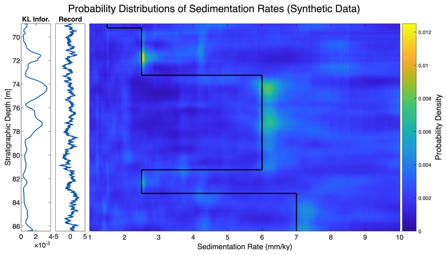
Figure 2 Probability density distributions of sedimentation rates computed from synthetic data with 200 % red noise (“Record” shown on the 2nd plot from left). The synthetic reference model is overlain (black curve) to illustrate the fidelity of the reconstruction. Visually, the reconstructed sedimentation rates closely reproduce the true reference model. However, the results also demonstrate that noise, together with ambiguity in assigning a given cycle to different target periods, can introduce artifacts and lead to multimodal sedimentation-rate probability distributions for a given depth. Information content (Kullbach-Leibler information) is shown in the left plot. Lower information content below 79 m depth, albeit with local peaks near 82.3 and 86.1 m, reflect fewer and/or less pronounced peaks within the sliding window.

Considering the relatively high noise level, the reconstruction of the true sedimentation rates is excellent. Abrupt changes in the sedimentation rate of about a factor three occur at 70, 74, 81, and 83 m, all of which are accurately captured by the AstroComb algorithm (Fig. 2). Sedimentation rates are not “smoothened”, but the timing of the abrupt change appears uncertain.

However, the test also illustrates how the probability distribution outside the correct sedimentation rate is not invariable or zero. In fact, artifacts (mathematically possible, but incorrect sedimentation rates) are introduced by the noise, the variability of the true model, window size, and the non-linearity of the problem. Some of these artifacts show up as spurious parallel features that could potentially be misinterpreted as representing true sedimentation rates. This highlights a key challenge in cyclostratigraphic analyses: a given cycle may be interpreted as corresponding to different target periods, resulting in a multimodal sedimentation-rate probability distribution. Nevertheless, the highest probability remains associated with the true reference model (Fig. 2). The Kullback-Leibler information content varies along stratigraphic depth with high information content at intervals where the sedimentation rate is constant across the window size (3.3 m) and low where the sedimentation rate changes within the window. In any case, we note that the algorithm identifies the true (reference) sedimentation rates despite the high noise level, and that it reconstructs the large discontinuities between layers of constant rates quite well, with lower probability near abrupt sedimentation rate changes. For comparison, we also processed a pure noise signal (see Fig. 3) to demonstrate that the algorithm is stable under such conditions, and will not produce spurious solutions with any significant probability.

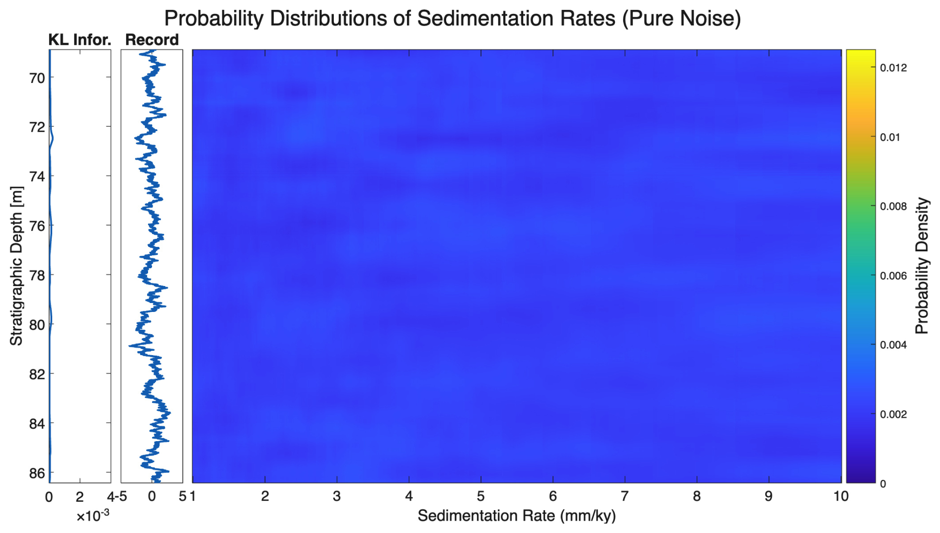
Figure 3 Probability density distributions of sedimentation rates computed from a pure noise signal (“Record” shown on the 2nd plot from left). Note the relative flatness of the posterior distributions, and the low values of the Kullback-Leibler information, relative to the synthetic data in Fig. 2.

This study demonstrates that the AstroComb method extends the spectral misfit minimization strategy in a probabilistic framework, handling uncertainty propagation and parameter tuning with statistical rigor.

3.2 Real world data from the late Cambrian Alum Shale Formation

To illustrate the application of the multichannel, probabilistic Milankovitch period detector, AstroComb, we analysed high-resolution XRF data from a ∼ 21 m long interval (67.2520–88.0744 m) of the Fågeltofta-2 drill core through the Alum Shale Formation in southern Sweden obtained by Sørensen et al. (2020). Briefly, the XRF data was collected using an ITRAX core scanner from Cox Laboratories with 30 kV voltage and 50 mA current on a Rh tube. The XRF measurements were collected with a high scanning resolution of 0.2 mm along the core and relatively long exposure time (7 s per scan), producing signal reported as concentrations for 22 elements, incl. Al₂O₃, SiO₂, S, K₂O, CaO, TiO₂, V, MnO, Fe₂O₃, Ni, Cu, Zn, Ge, As, Rb, Sr, Y, Zr, Mo, Ba, Hf, and U. This extensive elemental dataset formed the basis for the spectral analysis. Figure 4 shows a subset (the top 40 mm) of the data from ∼ 19 m of core, yielding ∼ 90 000 measurements.

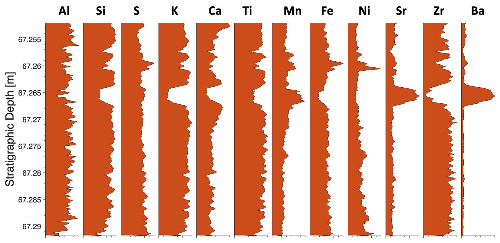
Figure 4 A selection of concentration profiles of the Fågeltofta-2 core, measured via XRF core scanning at 0.2 mm resolution. The records are all normalized to have the same maximum amplitude in the plot. The dataset spans approximately 19 m of stratigraphy and comprises ∼ 90 000 individual measurements. Several profiles show well-developed quasi-periodic oscillations, which serve as the primary proxy for detecting orbitally forced sedimentary cycles in the subsequent astrochronological analysis.

3.2.1 Using one channel

We selected Al as the primary input because of its robustness as a proxy for detrital input and its strong spectral structure in preliminary analysis (Sørensen et al., 2020; Zhao et al., 2022). The depth series was detrended with a linear function. AstroComb was run using a window length of 3.3 m, stepped every 0.2 mm.

The bulk sedimentation rate was a priori found within a range of realistic sedimentation rates from 1.0 to 10.0 mm kyr⁻¹. As output, we show the a posteriori probability distribution of the sedimentation rates versus stratigraphic depth (Fig. 5), and selected spectral fits for each 2 m in the core (Fig. 7). The Kullback–Leibler information measure at each depth z indicates that the Al record above 76 m contains a stronger Milankovitch signal than the deeper intervals of the core. This corresponds to an approximately fourfold improvement in the fit between the data and the target spectrum above 76 m. Overall, Fig. 5 suggests that Milankovitch cyclicity is present throughout the core, as indicated by the non-zero information content, while sedimentation rates appear to vary across the section.

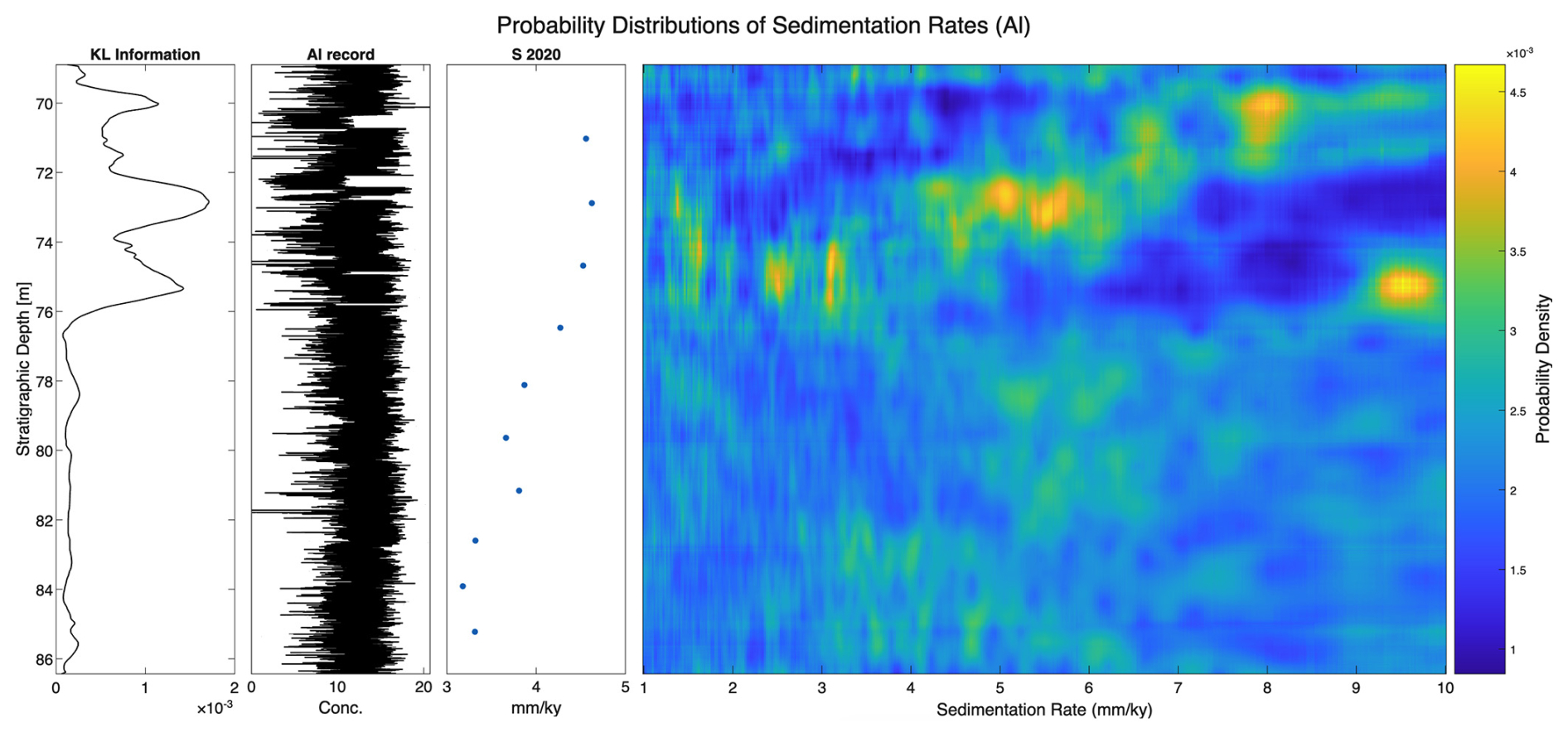
Figure 5 Sedimentation rate probability distribution for the Fågeltofta-2 core based on the Al record. The information content about Milankovitch cycles contained in the XRF data is quantified by the Kullback-Leibler measure.

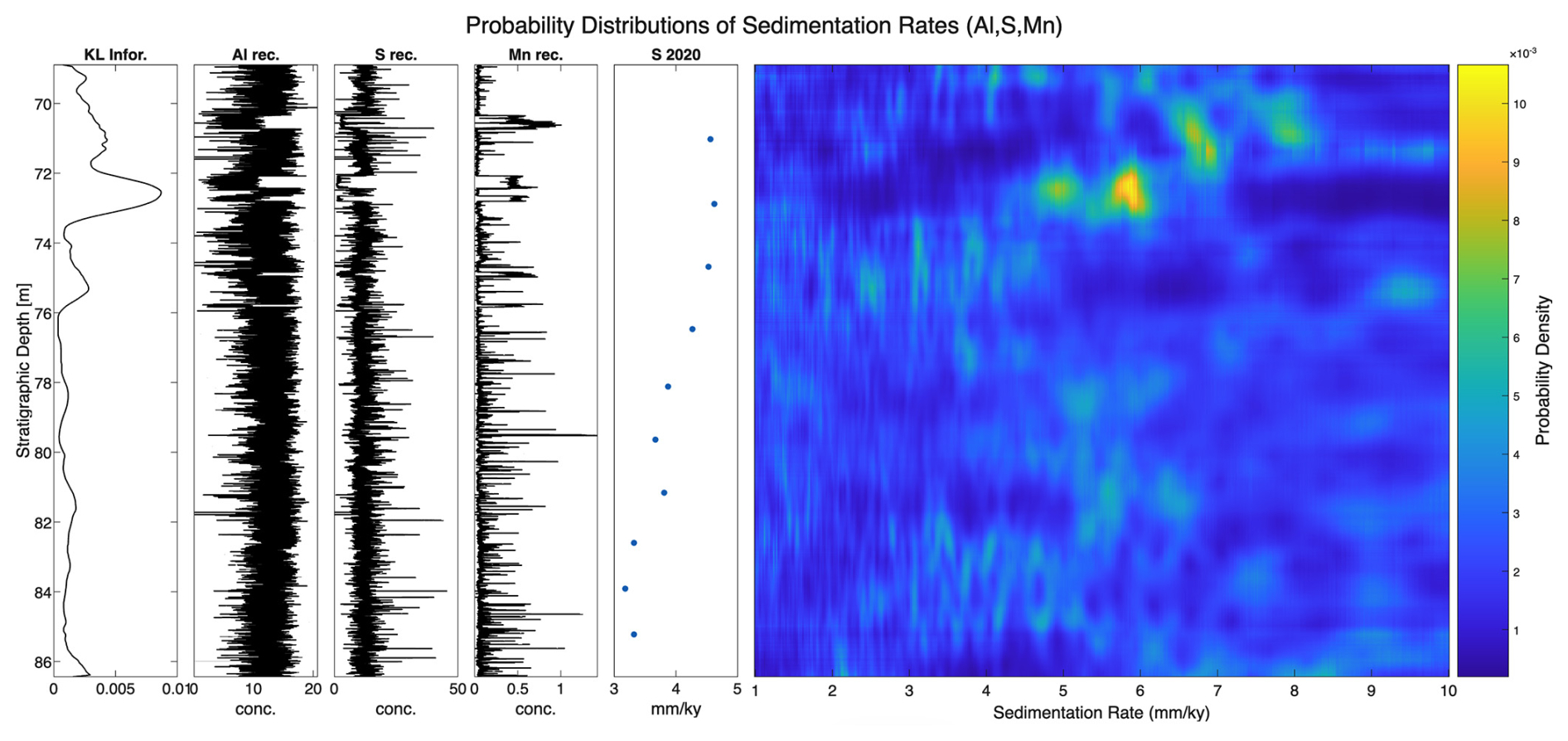
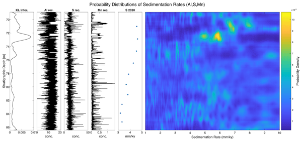
Figure 6 Probabilistic analysis of sedimentation rates in the Fågeltofta-2 core, based on simultaneous processing of S, Al, and Mn. Comparing to Fig. 5 it is clear that this multi-channel analysis has provided a higher resolution with more distinct peaks in the probability densities. Below 76 m, the information content is smaller where spectral peaks are few and/or less pronounced.

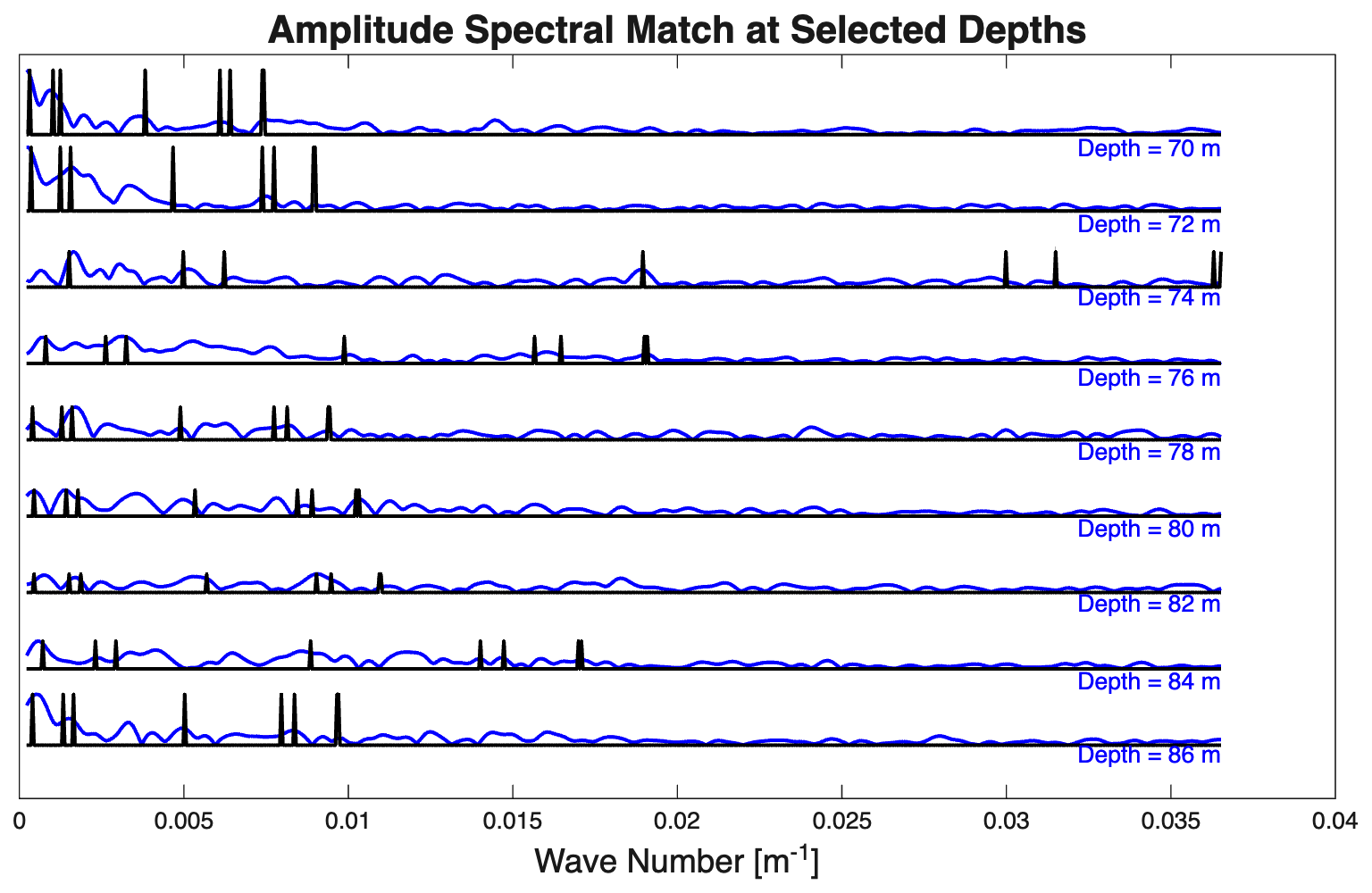
Figure 7 Spectral match at selected stratigraphic depths in the Fågeltofta-2 core. For every 2 m, the spectral lines corresponding to the best Milankovitch match are plotted (black) together with spectra of the Al content (blue) observed in windows centered at the depth.

From the estimated sedimentation rates, a Milankovitch timescale and its uncertainty was derived (Fig. 8), using the age of 496.595 Ma, consistent with Sørensen et al. (2020), at a stratigraphic depth of 86.005 m as a reference.

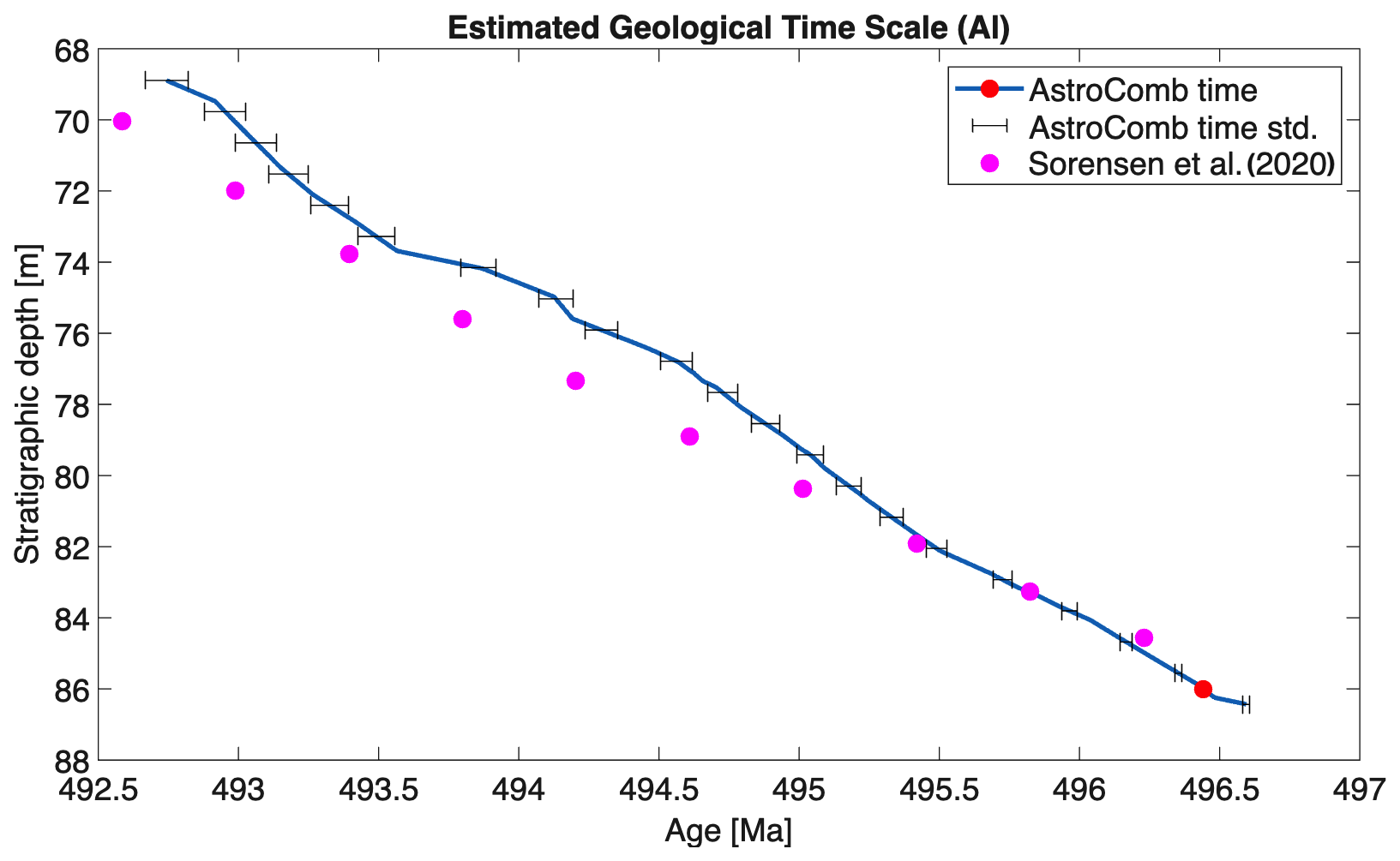
Figure 8 Estimated geological timescale and its uncertainty (standard deviation of a Gaussian approximation to the posterior near the computed time), based on probabilistic estimation of instantaneous sedimentation rates from the Al record in the Fågeltofta-2 core. Each time is a MAP estimate computed under the assumption of independency between neighbouring layers. The timescale is anchored at 86.005 m, corresponding to 496 595 kyr (Sørensen et al., 2020). This anchor is marked with a red circle on the graph.

This timescale enables the estimation of relative geological ages across the core, and allows depth-indexed chemical data to be analysed in the temporal domain, significantly enhancing our ability to interpret environmental transitions over geological timescales.

3.2.2 Using multiple channels

To demonstrate the capability of AstroComb for multichannel analysis, we applied the algorithm simultaneously to the S, Al, and Mn records. A central requirement in multichannel cyclostratigraphy is that the selected elemental channels provide independent information. Often elements or element ratios are used as channels. Yet, XRF elements also covary because they share mineral hosts, are affected by dilution, or are linked through mathematical relationships, and such covariance can create a misleading impression of increased certainty rather than reflecting independent signals of Milankovitch forcing. For this reason, it is important to choose elements that are not cohosted, not simple dilutions of one another, and not strongly coupled, a choice that relies on expert knowledge of mineralogy and geochemistry. For example, Al, S, and Mn meet these criteria in the Alum Shale. Although Al and S are often anti-correlated, earlier studies demonstrate that each element records Milankovitch periodicities in intervals where the other does not (Sørensen et al., 2020; Zhao et al., 2022), indicating that their orbital signals are not only products of dilution or other non-orbital processes.

The multichannel result, shown in Fig. 6, displays a clear improvement in spectral resolution compared to the single channel analysis in Fig. 5, especially in the top of the studied core interval. High probabilities increase, low probabilities decrease, and several secondary peaks that previously suggested alternative solutions are reduced or absent. The information content follows the same general pattern as before but increases by roughly an order of magnitude when three channels are used instead of one. The corresponding time scale is shown in Fig. 9.

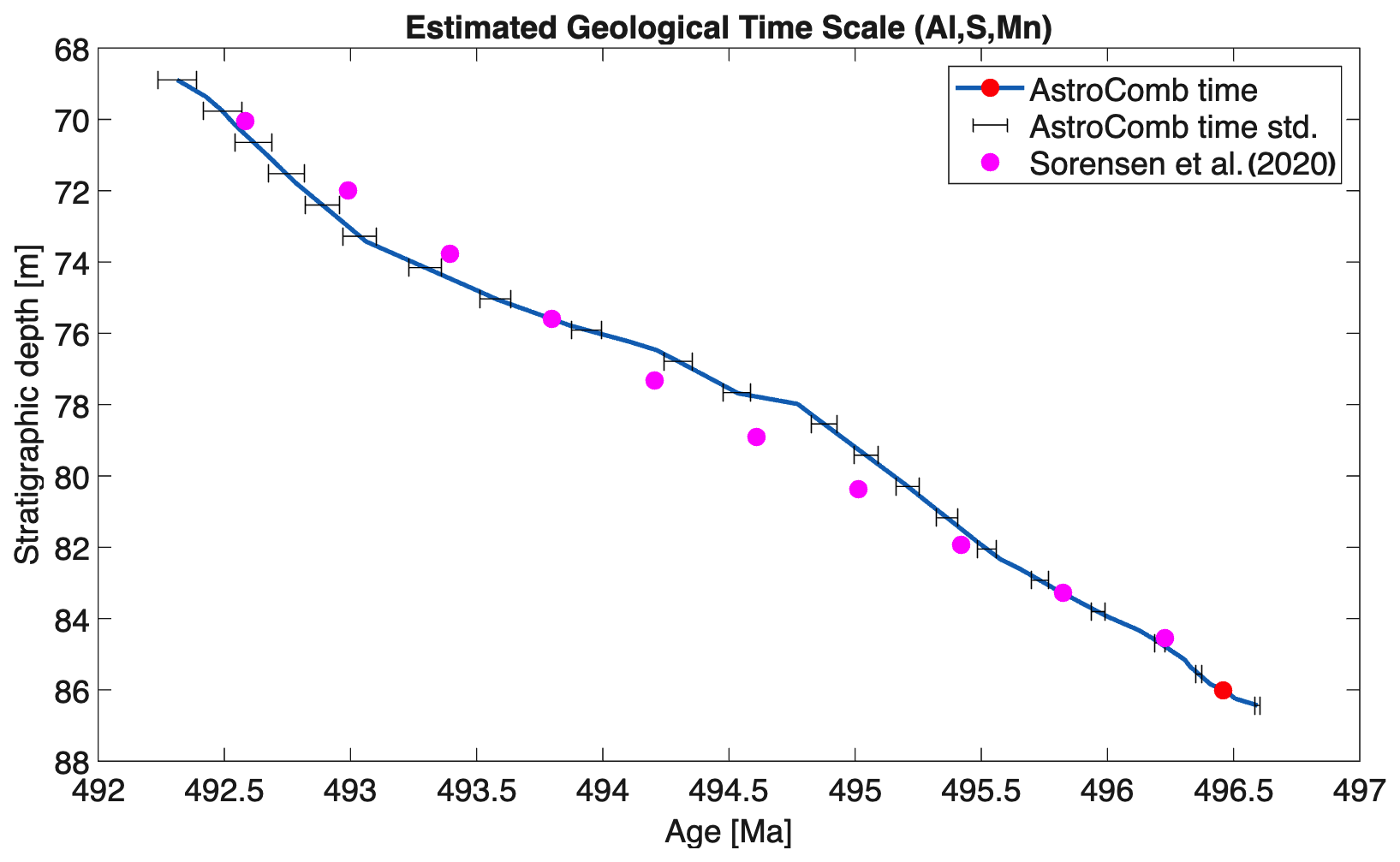
Figure 9 Timescale computed from the multi-channel data using the S, Al and Mn records. See Fig. 8 caption for further details.

These improvements in resolution are encouraging and support the use of AstroComb for probabilistic spectral inversion of high resolution XRF data for extracting geochronological information from ancient sedimentary archives.

4 Discussion

4.1 Interpretation of Results, and Methodological Limitations

The assumed orbital target periods are model-based. While the tuning strategy often relies on the 405 kyr eccentricity cycle as a stable chronometer, potential shifts in Earth’s rotational parameters due to e.g. tidal dissipation effects could introduce biases.

Our algorithm is based on the assumption that prior information about the spectral peak identification process can be provided, and that it adequately describes the way Milankovitch periods are identified by human analysts. Little prior information about the unknown sedimentation rates is used, meaning that the effective prior probability density is uniform (constant in a wide interval).

The fundamental output of the algorithm is the posterior probability densities shown in Figs. 5 and 6. It is apparent from these distribution that multiple, valid solutions to the problem exists. For example, in the single-channel data, in parts of the depth interval 74–78 m, there is a choice between rather low (∼3.2 mm kyr⁻¹) sedimentation rates and rather high values (∼9.8 mm kyr⁻¹). When calculating the geological timescales (time-depth curves) a choice between these solutions must be made, and the current version of the algorithm calculates the time independently for every layer based on the maximum a posteriori (MAP) estimates, that is, the sedimentation rates with the highest values of the posterior probability density (see Figs. 8 and 9). However, expert knowledge about the sedimentary system could be added as a non-uniform prior on the sedimentation rates, and this could well change the MAP solution. For example, one may add that the sedimentation rate cannot jump arbitrarily between adjacent layers in the case where two sedimentation rates are roughly equally probable within a stratigraphic interval. Using such information can be seen in Figs. 8 and 9, where we have plotted sedimentation rates from previous studies (Sørensen et al., 2020; Zhao et al., 2022), where higher values for the sedimentation rates in the depth interval 74–78 m has been chosen based on prior knowledge not included in AstroComb. As a result, the age-depth models deviate in this interval (Fig. 8).

There are also some fundamental assumptions behind Milankovitch analysis that apply to any method. Milankovitch cycles are (quasi-)periodic, but not sinusoidal. This means that a hypothetical, noise-free Milankovitch spectrum will, in general, contain spectral components outside the main Milankovitch frequencies (Sinnesael et al., 2018). These components are generally disregarded in Milankovitch analysis programs, including AstroComb. More seriously, the Earth's sedimentary system is highly nonlinear and therefore could produce additional periods that are sums and differences of the main Milankovitch cycles. The amplitudes of such periods could be significant, but they are ignored by our algorithm. For linear, as well as nonlinear sedimentary systems, even if we know the amplitudes of the input Milankovitch signal, the output amplitudes observed in boreholes are entirely unknown. This was the background for the way that we designed our spectral fit algorithm, e.g. making an analytical tool which is somewhat agnostic to the amplitude of the recorded periodicities.

Last, but not least, it is important to remember that Milankovitch cycle identification is a difficult problem. The signal-to-noise ratio is generally very low, and the problem is often similar to finding a needle in a hay stack. Such problems are prone to detrimental human biases, but AstroComb is designed with the aim of quantifying the analysis, and casting the problem as a probabilistic inference problem, so as to avoid such biases. The probability distribution presented here generally provides several plausible solutions for the sedimentation rates at given depths, allowing the user to choose based on geological/stratigraphic knowledge and clearly identify such choices.

4.2 Broader Implications

The AstroComb algorithm is a new unsupervised approach for identifying Milankovitch cycles in multi-channel data. The algorithm has discovered abrupt changes in sedimentation rate in the Fågeltofta-2 core, as opposed to smooth transitions, potentially guiding sedimentologist in reconstructing pulses of sedimentation from geological archives. This opens tantalizing new prospects for understanding relative sea level changes because the shifts in sedimentation rate in the Alum shale Formation (incl. Billegrav-2 and Fågeltofta) are correlated with the changes in relative sea level obtained from the sequence stratigraphy (Sørensen et al., 2020). Where previous sedimentation rate estimates obtained using eCOCO and a smoothing spline fit on visually profound periods in the wavelet spectrum unavoidably induced some degree of smoothing of the sedimentation rate that may give a false impression of the actual sedimentation rate changes, AstroComb delivers sedimentation rate changes that are not necessarily changing smoothly across stratigraphy.

As sedimentation rate is a fundamental parameter characterizing a sedimentary environment and a factor that serves as a first order control on organic matter preservation, AstroComb may help engaging sedimentologists with a new relative chronometer. Also, we envision to refine geochronology further by using it in combination with geochemical information about sedimentation rate changes.

5 Conclusions

The algorithm contributes methodologically to the field of deep-time astrochronology by offering a multi-channel, probabilistic method for estimation of astronomically constrained timescales. At the same time we offer critical quality control of the data, allowing the user to evaluate how much Milankovich information can actually be detected in the XRF-derived elemental records. The framework established here provides a robust platform for exploring the causes and consequences of climatic, geochemical, and evolutionary change in Earth’s early history.