the Creative Commons Attribution 4.0 License.
the Creative Commons Attribution 4.0 License.
 | 02 Dec 2025
Projecting management-relevant change of undeveloped coastal barriers with the Mesoscale Explicit Ecogeomorphic Barrier model (MEEB) v1.0
Andrew D. Ashton
Erika E. Lentz
Christopher R. Sherwood
Davina L. Passeri
Sara L. Zeigler
Models of coastal barrier geomorphic and ecologic change are valuable tools for understanding and predicting when, where, and how barriers evolve and transition between ecogeomorphic states. Few existing models of barrier systems are designed to operate over spatiotemporal scales congruous with effective management practices (i.e., decades/kilometers, referred to herein as “mesoscales”), incorporate important ecogeomorphic feedbacks, and provide probabilistic projections of future change. Here, we present a new numerical model designed to address these gaps by explicitly yet efficiently simulating coupled aeolian, marine, vegetation, and shoreline components of barrier evolution over spatiotemporal scales relevant to management. The Mesoscale Explicit Ecogeomorphic Barrier model (MEEB) simulates subaerial ecomorphologic change of undeveloped barrier systems over kilometers and decades using meter-scale spatial resolution and weekly time steps. MEEB applies simplified parameterizations to represent and couple key ecogeomorphic processes: dune growth, vegetation expansion and mortality, beach and foredune erosion, barrier overwash, and shoreline and shoreface change. The model is parameterized and calibrated with observed elevation, vegetation, and water level data for a case study site of North Core Banks, NC, USA. Simulated ecogeomorphic change in model hindcasts agrees well with observations, demonstrating both favorable skill scores and qualitatively correct behavior. We also describe an additional model framework for producing probabilistic projections that account for uncertainties related to future forcing conditions and intrinsic stochastic dynamics and demonstrate the probabilistic framework's utility with example forecast simulations. As a mesoscale model, MEEB is designed to investigate questions about future barrier ecogeomorphic change of moderate complexity, offering semi-qualitative predictions and semi-quantitative explanations. For example, MEEB can be used to investigate how climate-induced shifts in ecological composition may alter the likelihood of morphologic impacts or to generate probabilistic projections of ecogeomorphic state change.
- Article
(9238 KB) - Full-text XML
- BibTeX
- EndNote


Coastal barrier environments are of critical economic, ecologic, and cultural importance, but, as low-lying collections of mobile sediment, are constantly evolving under drivers of both chronic and event-based change. In the face of rising atmospheric temperatures, projected accelerated relative sea-level rise (RSLR; Sweet et al., 2022), and anticipated changes in tropical storm activity (e.g., Knutson et al., 2020), future barrier evolution remains uncertain. This uncertainty is further complicated by transformations in ecological assemblages related to global climate warming, which have become increasingly apparent within barrier systems in recent decades (e.g., Goldstein et al., 2018; Zinnert et al., 2016) and have the potential to fundamentally alter the morphology and behavior of coastal barriers (e.g., Reeves et al., 2022; Zinnert et al., 2019). An understanding of when, where, and how ecogeomorphic change in barrier systems is most likely to occur remains of paramount importance to coastal communities looking to prepare for and adapt to future change. Furthermore, the ability to capture future changes to barrier systems can help inform broader understanding of both the functional transformations we may anticipate across the broader coastal landscape, as well as whether protections coastal barriers provide to mainland settings will persist in the future.
Numerical models capable of simulating across a range of scenarios and conditions offer possibly the best opportunity to predict and understand coastal change and behavior. Prediction of historically unprecedented behavior will be important given uncertainties in future forcing conditions (e.g., RSLR, storm intensity) coupled with inherently complex nonlinear interactions (e.g., feedbacks, multistability) and stochasticity (e.g., storm occurrence, seed dispersal). Numerical models can inform active planning and management strategies for “undeveloped” barrier systems (i.e., those without sustained residential and/or commercial infrastructure and activity) that are typically intended to preserve and protect ecosystems, infrastructure, and natural resources; provide for human use; mitigate hazards; and inform public expectations.
Coastal management practices usually consider timescales of several decades into the future – often with regard to milestones of 2050 and 2100 CE defined by climate change science – over multiple kilometers of coastline. Amongst coastal managers and decision-makers, there is increasing demand for model projections that both explicitly take into account these spatiotemporal horizons and at the same time provide reliable and sufficiently quantitative predictions (French et al., 2016; Martin et al., 2023). Many models of barrier geomorphology and ecology exist as powerful tools for predicting event-based change or understanding fundamental behaviors and processes (Hoagland et al., 2023; Piercy et al., 2023). While these models provide useful insight to planning and decision-making processes, they tend to lack important features and components that are particularly relevant to the typical goals of management endeavors: management-relevant spatiotemporal scales (decades and kilometers) and resolutions (meters and weeks), feedbacks between key ecologic and geomorphic processes, and the ability to provide probabilistic projections of future change.
Numerical models of barrier evolution can be arranged along a continuum between micro and macro scales (Hoagland et al., 2023; Murray, 2003). What we herein consider microscale models (e.g., XBeach, Roelvink et al., 2009; Delft3D, Lesser et al., 2004; COAWST, Warner et al., 2008), also commonly referred to as event-based or simulation models, typically simulate coastal change over hours to years and up to hundreds of meters. These models tend to be built upon highly realistic expressions of the underlying physics and incorporate as many system processes as practical while striving to simulate a particular place or set of conditions with as much quantitative accuracy (predictive skill) as possible (Murray, 2003; Sherwood et al., 2022). As such, microscale models typically require relatively large computational resources, observational or experimental data for model initialization and testing, and careful calibration of important model coefficients (e.g., Windsurf, Itzkin et al., 2022). In contrast, macroscale models (e.g., CoastMorpho2D, Mariotti, 2021; Barrier3D, Reeves et al., 2021; BIT, Masetti et al., 2008; BRIE, Nienhuis and Lorenzo-Trueba, 2019a), often referred to as exploratory or reduced-complexity models, operate over temporal scales of decades to millennia and over spatial scales up to thousands of meters, typically with coarse spatial resolutions ≥ 10 m. Macroscale models simplify systems to focus on essential, emergent processes, often with the goal of exploring and explaining large-scale behavior (Murray, 2003). As such, larger-scale models tend to use synthesized representations of natural phenomena that average over ecogeomorphic processes and features occurring at much smaller spatiotemporal scales, providing the most direct explanations and likely the most reliable predictions of larger-scale phenomena (Murray, 2007). Macroscale models also tend to use idealized (e.g., LTA14, Lorenzo-Trueba and Ashton, 2014) or equilibrium (e.g., GEOMBEST, Stolper et al., 2005) morphologies meant to represent generalized conditions or behaviors rather than specific real-world locations.
There is a dearth, however, of mesoscale models that occupy the continuum between micro- and macroscale endmembers. Few models or model frameworks of coastal barrier environments are designed to simulate over years to decades and hundreds to thousands of meters and with meter-scale spatial resolution. Notable exceptions include DUBEVEG (Keijsers et al., 2016) and the Coastal Dune Model (Durán Vinent and Moore, 2015), which simulate decadal ecologic and geomorphic evolution of beach and dune environments, and ISLAND (Rastetter, 1991) and the model of Robson et al. (2024), which model decadal vegetation-habitat interactions across a barrier; however, these models lack full representation of the entire barrier system and/or key processes (e.g., overwash) needed for holistic assessments and relevant mesoscale projections of barrier evolution. The polarity of spatiotemporal scales among existing coastal barrier models likely exists because of contrasting goals, assumptions, and modeling techniques of micro- and macroscale models (Murray, 2003); the sheer number of processes that could be important for driving coastal change (van Maanen et al., 2016); a lack of decadal observational data needed to develop mesoscale parameterizations and evaluate mesoscale models (French et al., 2016; Hoagland et al., 2023); and nascent theory on model up-scaling and down-scaling, with up-scaling approaches (i.e., using microscale models in meso- or macroscale applications) particularly limited by high computational costs and the potential for imperfections in reductionist microscale parameterizations compounding over much larger scales, thereby preventing reliable quantitative results (Murray, 2007; French et al., 2016). However, coastal management practices typically consider timescales on the order of several decades into the future, stemming largely from the well-established climate and sea-level rise horizons of 2050 and 2100 CE. Additionally, continuous, spatially explicit coverage of an area of interest in both the cross-shore and alongshore dimensions, as well as weekly to annual (temporal) and meter to decameter (spatial) resolutions, are needed to inform comprehensive management scenarios (e.g., Martin et al., 2023). As such, barrier models operating at mesoscales are perhaps most promising for addressing the needs of strategic coastal planning and decision-making (French et al., 2016; van Maanen et al., 2016; Woodroffe and Murray-Wallace, 2012).
Incorporation of ecological dynamics and their feedbacks with geomorphic processes is also underrepresented in models of coastal barrier evolution (Hoagland et al., 2023; Piercy et al., 2023). Bidirectional physical-ecological feedbacks within coastal barrier environments are especially relevant at mesoscales, where vital ecogeomorphic behaviors tend to emerge. At much smaller scales (i.e., years and 101 m, or smaller), spatiotemporal change in the size, location, or type of herbaceous and woody vegetation found in coastal barrier environments tends to be prohibitively small for generating dynamic ecogeomorphic interactions and feedbacks; at much larger spatiotemporal scales (i.e., centuries or millennia and 101 km, or larger), the influence of vegetation on geomorphic processes tends to become increasingly difficult to recognize (Larsen et al., 2021). It is well documented that ecogeomorphic interactions and feedbacks are fundamental to coastal barrier systems, from the stimulation of dune-growing grasses in response to sand deposition (e.g., Zarnetske et al., 2012) to woody shrubs obstructing overwash flow (Reeves et al., 2022; Zinnert et al., 2019), yet these interactions are often neglected in barrier models. Modeling approaches that implicitly incorporate the effects of vegetation through static parameterizations, such as landcover roughness coefficients (e.g., Passeri et al., 2018), are typically not appropriate for addressing questions related to meso- or macroscale evolution where the configuration of vegetation is expected to change across space and time. However, some models of barrier systems have begun to include physical-biological feedbacks by explicitly simulating the spatiotemporal variation of vegetation communities across coastal barrier landscapes and their couplings with physical processes (e.g., ISLAND, Rastetter, 1991; Barrier3D, Reeves et al., 2022; DUBEVEG, Keijsers et al., 2016; Coastal Dune Model, Durán Vinent and Moore, 2015; GEOMBESTSeagrass, Reeves et al., 2020). Given the sensitivity of coastal ecosystems to changes in climatic forcings and potential ecological transformations arising from global climate change (e.g., Goldstein et al., 2018; Jackson et al., 2019; Zinnert et al., 2016; Lucas and Carter, 2010), ecogeomorphic interactions are likely to play an increasingly prominent role over the next century. Including dynamic ecogeomorphic couplings within coastal barrier models therefore improves the performance of mesoscale projections and confidence in their findings.
Most barrier-evolution models provide only deterministic projections, despite often considerable uncertainty in projections of macroscale drivers of coastal change (e.g., sea-level rise, storminess, atmospheric temperature) and the inherent randomness of natural phenomena (e.g., storm timing). Significant uncertainties also arise from future human activities and decision-making (e.g., McNamara and Lazarus, 2018), but coupled human–natural considerations are beyond the present scope of this model. While deterministic models inherit the uncertainties of model input forcings, model approaches that account for the probabilistic nature of the drivers of barrier evolution (e.g., Lentz et al., 2016; Bamunawala et al., 2021; Wainwright et al., 2015) can potentially provide a more holistic assessment of future change to better inform management activities (e.g., van der Lugt, 2019).
Here we present the Mesoscale Explicit Ecogeomorphic Barrier model (MEEB), which simulates the spatially explicit ecogeomorphic change of undeveloped barrier systems over several decades and kilometers. MEEB tackles the separation of scales among pre-existing barrier models by explicitly yet efficiently simulating aeolian, marine, shoreline, and vegetation components of a coastal barrier segment. Additionally, the model incorporates uncertainties related to future drivers and the inherent stochasticity of natural processes to produce probabilistic projections of future change across space and time. The goal of MEEB is to balance management needs for spatially explicit, quantitative predictions with mesoscale (multi-decadal and multi-kilometer) projections and related uncertainties while accounting for real feedbacks between ecosystems, geomorphology, and hydrodynamic processes. To accomplish this, we use a hybrid model architecture that incorporates certain model parameterizations of higher mechanistic complexity, only as far as to produce mesoscale behaviors anticipated to be important, with more simplified, larger-scale parameterizations that most reliably capture the collective effects of many processes happening at much smaller scales (Thornhill et al., 2015; French et al., 2016; Murray, 2007). As an important part of our hybrid approach, we also explicitly and robustly test and calibrate the relatively simple model parametrizations with observational data. MEEB is not suitable for predicting subtle shifts in elevation or vegetation, nor for explaining the reconfiguration of a landscape or its behaviors. Rather, MEEB is designed to answer questions of moderate complexity regarding when, where, and how ecogeomorphic change is likely to occur, with correspondingly moderate levels of both predictive (quantitative) and explanatory (qualitative) power. In the sections that follow, we provide a description of the model processes and parameterizations; detail data integration and calibration procedures; and assess and discuss model performance, parameter sensitivities, and appropriate use.
The Mesoscale Explicit Ecogeomorphic Barrier model (MEEB; Reeves, 2025a) resolves cross-shore and alongshore variations in topography and ecology to simulate the ecogeomorphic evolution of an undeveloped barrier or barrier segment (Fig. 1). MEEB operates with a planform grid resolution on the order of meters and 0.02 years (7.3 d) timesteps, and can run for years to decades over 100–102 km of barrier shoreline. We use a grid resolution of 1 m as herbaceous species in barrier ecosystems typically grow in clusters on the order of 1 m2 in size, though the model produces qualitatively similar output with resolutions up to 2 m (resolutions outside this range have not been tested). Spatial resolution of the model is dictated in large part by the typical size of the vegetation growth pattern, as the vegetation imposes a characteristic length scale on the resultant aeolian morphology (Nield and Baas, 2008a). Therefore, we do not suggest adopting a grid resolution outside the 1 to 2 m range. The model is written in Python and can be run on PC, Macintosh, and Linux operating systems. The typical runtime for a 10-year simulation of a 1 km-long barrier segment with 1 m grid resolution is approximately 40 to 80 min, or approximately 10 to 20 min with a grid resolution of 2 m. Memory usage depends strongly on domain size, grid resolution, and the frequency and type of saved model output. An individual deterministic simulation in MEEB is run on an individual core, while our probabilistic framework runs batches of deterministic simulations in parallel across multiple cores (as many as allocated); a high-performance computing cluster is recommended for probabilistic simulations spanning >10 km of shoreline. The relative balance between spatiotemporal resolution, spatiotemporal extent, and efficiency makes the model ideal for studying mesoscale barrier evolution.
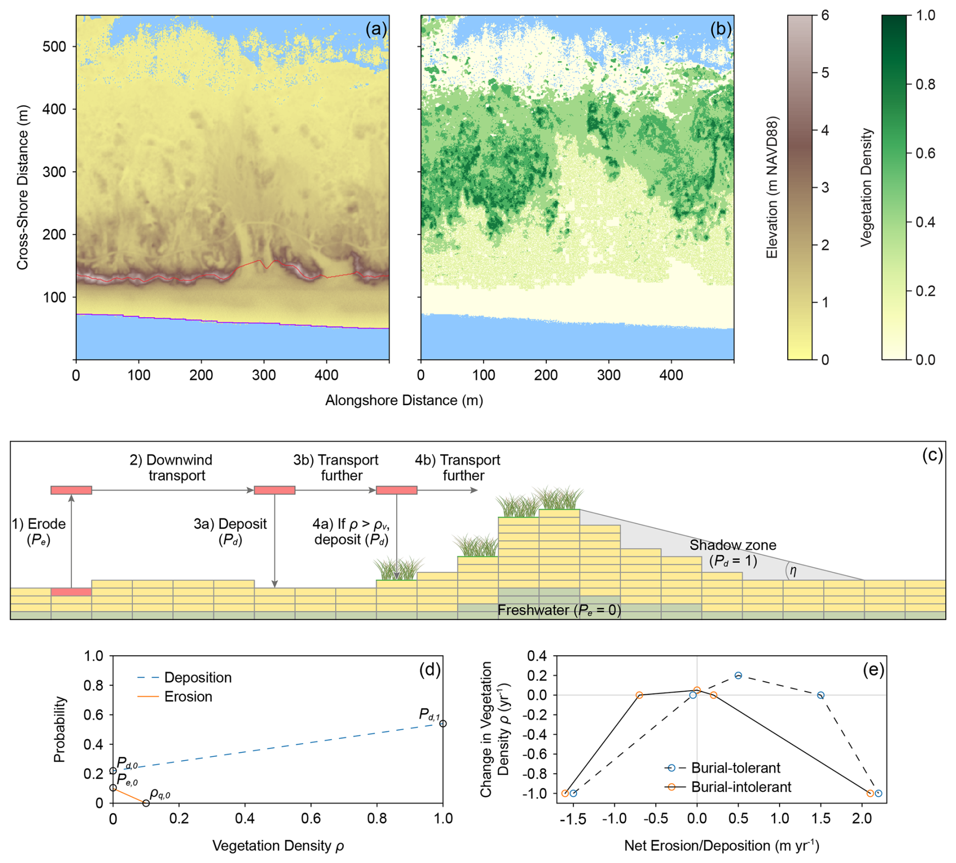
Figure 1MEEB model configuration. (a) Example model elevation domain, annotated with the foredune crestline (red) and ocean shoreline (purple), and (b) corresponding vegetation density domain. (c) Schematic diagram of sand slab transport in the Aeolian component of MEEB, wherein slabs are stochastically entrained, transported downwind, and either deposited or transported further; each of these processes is affected by vegetation, shadow zones, and the water table. (d) Probabilities of slab erosion and deposition as a function of vegetation density. (e) Annual vegetation growth for burial-tolerant and burial-intolerant species types as a function of the annual net sedimentation balance.
The model tracks changes in elevation and vegetation density and type through space and time across separate elevation and vegetation domains. Ecogeomorphic evolution in MEEB is limited to areas above the mean high water (MHW) elevation; intertidal and subaqueous environments are therefore not explicitly modeled. The MHW elevation changes each model iteration according to the RSLR rate, which is constant through time (given that RSLR projections up to the year 2050 can be closely approximated as linear). A groundwater lens is modeled as a function of the subaerial topography and may intersect depressions in the land surface as ponds. Due to complexities in modeling inlet dynamics, MEEB is not capable of simulating portions of a barrier chain with or directly influenced by active tidal inlets or shoals from recently abandoned inlets. Additionally, MEEB assumes the barrier system is composed entirely of unconsolidated sand. MEEB is initialized with elevation, vegetation cover, and high-water event climatology data, which we discuss in Sect. 3 below. All model parameters and dependent variables, along with their units and values, are listed in Appendix A.
2.1 Model Framework and Time-stepping
Four components comprise the MEEB framework: Aeolian, Marine, Shoreline, and Vegetation. These four components operate in succession within a model timestep but act at different timescales, so not all components are involved in each model iteration (Fig. 2). A model year begins with the Aeolian component, which occurs every model timestep (Δta=0.02 years or ∼ 7.3 d). The Aeolian component determines the entrainment, transport, and deposition of sand across the barrier surface resulting from wind and dependent on the vegetation cover and topography. This Aeolian process repeats itself twice, updating the elevation domain each iteration, and is then followed by the Marine component, which occurs every second model timestep (Δtm=0.04 years or ∼ 14.6 d) to correspond to a spring–neap tidal cycle and because storm systems can potentially last more than 7 d. The Marine component determines how sediment is transported across the beach, dune, and barrier interior from swash, collision, and overwash processes during a high-water event (HWE), defined as an event in which the total water level (TWL; the sum of tide, surge, and wave runup) exceeds MHW. These HWE-induced processes are influenced by the topography, vegetation cover, and HWE water elevation and duration. In addition to updating the elevation domain, the Marine component also updates the vegetation domain by converting previously vegetated cells to bare wherever inundated. The Shoreline component, which also occurs every second model timestep (Δts=0.04 years or ∼ 14.6 d), directly follows the Marine component. The Shoreline component determines the position of the MHW ocean shoreline according to RSLR and cross-shore and alongshore sediment transport, and adjusts the shoreline by adding (accretion) or removing (erosion) elevation. This sequence of two Aeolian iterations, one Marine iteration, and one Shoreline iteration repeats for a total of 25 times in the model year. Thereafter, the full model year is completed with execution of the Vegetation component, which occurs every 50 model timesteps (Δtv=1.0 year or 365 d). The Vegetation component determines the expansion of plants into previously bare cells and changes in vegetation density (growth or decay), the latter of which is dependent upon the net erosion/deposition over the course of the preceding year. The cycle then restarts with the updated elevation and vegetation domains for the next model year (Fig. 2).
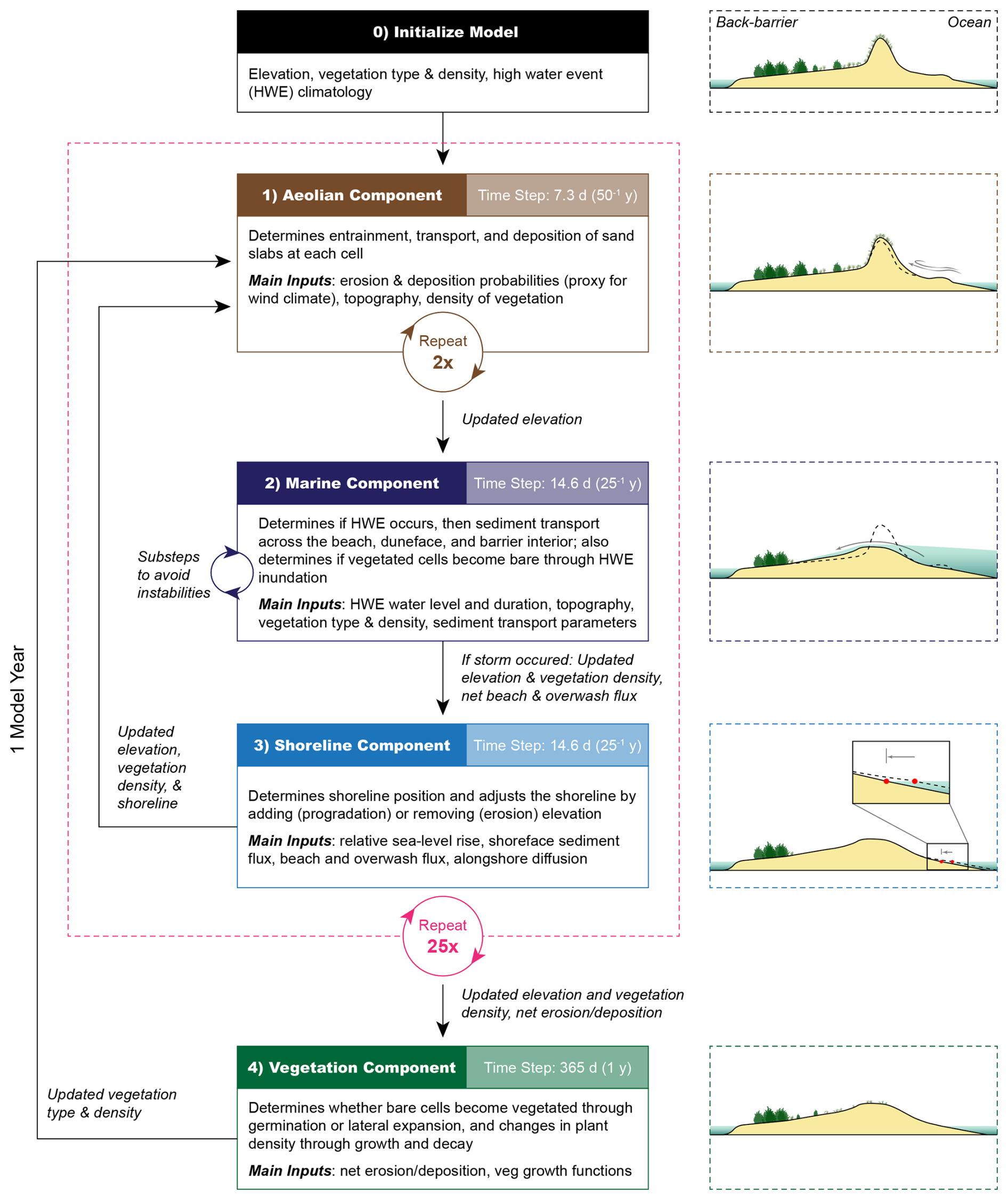
Figure 2Flow diagram and schematic illustrations of model process domains across one model year in MEEB.
2.2 Aeolian
MEEB uses a cellular model of aeolian morphologic development in which slabs of sand are probabilistically entrained, transported, and deposited based on a set of rules that capture the effects of real-world aeolian processes. Our Aeolian component stems from the aeolian side of the DUBEVEG model (Dune, BEach, and VEGetation; Keijsers et al., 2016), which itself builds upon earlier cellular slab-based dune models (Baas, 2002; Baas and Nield, 2007; Werner, 1995). The Aeolian component in MEEB updates the topography 50 times a year (time step Δta=0.02 years or ∼ 7.3 d).
During each Aeolian iteration, every cell in the domain is polled once for entrainment based on a probability of erosion (Pe) ranging from zero to one, as discussed below. If entrainment in a cell is probabilistically determined to occur, a slab of sand with a fixed height (Hs) is removed from the entrainment site and transported downwind according to the saltation length (Ls). A probability of deposition (Pd) at the receiving cell determines whether the slab will deposit or be transported downwind again (Fig. 1c). As a proxy for weekly time-varying wind speeds, we stochastically vary Ls each Aeolian iteration by drawing from a simple uniform distribution centered around a mean (here, 5 ± 2 m). As a proxy for the longer-term (annual- or decadal-scale) average strength of the wind climate, the maximum potential aeolian transport volume flux (qa,max) can be calculated following Nield and Baas (2008a) as:
Changing the values Pe and Pd, as well as Hs and Ls, therefore captures the effects of stronger or weaker wind climates. Wind direction – onshore, alongshore down, offshore, or alongshore up across the gridded domain – is determined by weighted random choice for each Aeolian iteration, with the probability of each of the 4 directions (PWD) summing to 1. The collective effects of oblique winds are roughly captured with asymmetric multidirectional transport directions (cf. Nield and Baas, 2008a). At the end of each Aeolian iteration, angles of repose for bare and vegetated cells are maintained by avalanching slabs in the direction of steepest descent. The Aeolian component uses open boundary conditions wherein slabs of sediment can be transported out of the lateral edges of the model domain (sediment can be imported into the domain within the Marine component of the model, as described below).
Probabilities of erosion and deposition vary across the landscape as a function of ecological and physical factors. Wind shadow zones, wherein Pe=0 and Pd=1, extend from the lee side of topographic peaks as determined by the shadow angle η (Fig. 1c). Where elevation is below MHW or the elevation of a groundwater lens, Pe=0 and Pd=1. Assuming that the groundwater surface typically resembles a subdued reflection of the topography, the groundwater surface in MEEB is determined as a proportion of the topographic surface height above MHW (Fig. 1c; Galiforni Silva et al., 2018) that has been smoothed by a Gaussian filter (with a standard deviation for the Gaussian kernel, σ, of 12 m). Groundwater can intersect topographic depressions as surface ponds (MEEB does not flatten the water surface in ponds given that Pe=0 and Pd=1 regardless). Additionally, the presence of vegetation cover reduces the probability that a slab will be eroded and increases the probability that a slab will be deposited in proportion to the vegetation density (ρ) of each cell (Fig. 1d). Pe decreases linearly from its maximum (Pe,0) when ρ=0 to 0 when ρ=ρq0, the vegetation density at which entrainment of sand becomes effectively negligible. Where vegetation is present in cells between the entrainment site and receiving site along the transport path, entrained slabs are polled for deposition at each intermediary vegetated cell if ρ is greater than a threshold value ρv (Teixeira et al., 2023). To account for the effects of vegetated cells on the local wind field of neighboring unvegetated cells, the Aeolian component of MEEB uses a copy of the current vegetation density domain that has been lightly smoothed with a Gaussian filter (σ=3 m).
2.3 Marine
High-water events (HWEs) occur intermittently in MEEB, causing changes to the subaerial morphology and ecology. We define HWEs as all events in which the total water level exceeds MHW. As discussed below, MEEB uses separate – but coupled – model formulations seaward and landward of the dynamic foredune crestline (described in Sect. 2.3.1 below) to simulate ecogeomorphic change from HWEs. The model can run hindcast simulations using time series of observed HWEs as input or run forecast simulations with a stochastic HWE environment developed from the time series of observed HWEs. Our methodology for the observational HWE time series and stochastic HWE environment is described in Sect. 3.3, below.
Every 25−1 years (Δtm=0.04 years or ∼ 14.6 d), MEEB determines whether a HWE occurs depending on the observed time series (for hindcasts) or a probability of occurrence dependent on the time of year (for forecasts). If no HWE is determined to occur for a Marine iteration, no marine processes take place (i.e., the landscape remains unaltered) and MEEB proceeds directly to the Shoreline component of the model. If a HWE is determined to occur for a Marine iteration, the HWE is described by a total water level (TWL), which can vary alongshore according to the local beach slope, and a duration (in hours). In the stochastic HWE environment, the conditions of each event are chosen randomly from a list of synthetic HWEs; the probability of occurrence and average intensity (TWL and duration) of the list of synthetic HWEs, however, remain constant over the course of each simulation. For simplicity, and because our identification of HWEs tend to lump multiple tidal cycles of an event together, MEEB allows a maximum of one HWE to occur during each 0.04 years (14.6 d) interval.
2.3.1 Dune crest location
MEEB uses separate formulations for HWE-driven morphologic change landward and seaward of the foredune crest, therefore requiring the alongshore-continuous location of the foredune ridge. MEEB identifies the cross-shore locations of the foredune crest (xD) for every dy alongshore – the foredune crestline – using a multi-step process that considers the general trend of the foredune crest location to identify gaps in the crestline where the dune would be most likely to (re)form. First, the algorithm finds the cross-shore locations of the elevation maximum for an elevation domain that has been smoothed in the alongshore dimension using a large-window (150 m) moving average. This maximum elevation crestline is smoothed again with a Savitzky-Golay filter (window length = 75 m), resulting in a demarcation that gives the broad, general trend of where the foredune crest is or would tend to be (in the case of gaps in the foredune) located within the barrier domain. Next, using the original non-smoothed elevation domain, the algorithm finds the cross-shore location of the dune-crest peaks within a 25 m buffer of this broad crest trendline. Dune-crest peaks are selected as the most-seaward peak of a profile with a minimum backshore drop of 0.6 m (Itzkin et al., 2020; Mull and Ruggiero, 2014). If no peak is found within a profile, the algorithm selects the location from the nearest neighboring peak and the location alongshore is considered a gap in the foredune crestline. Lastly, a Savitzky-Golay filter is applied again with a smaller window length (11 m) to produce the continuous foredune crestline.
2.3.2 Ocean shoreline to foredune crest
MEEB uses an equation for cross-shore net sediment transport between the surf-swash boundary and the foredune crest to simulate HWE processes seaward of the foredune crest. Based on Durán Vinent and Moore (2015) and, by extension, Larson et al. (2004a), the deposited volume of sediment at cross-shore location x, qx, each iteration is equal to
with βeq the representative equilibrium slope of the beach, βx the local slope at the cross-shore location x, Ztwl the TWL elevation, Zx the elevation at the cross-shore location x, and Te a calibration coefficient for the erosive timescale (see Appendix A for a list of model parameters and dependent variables, their units, and values used herein). Sediment transport for each HWE iteration is calculated from the ocean shoreline up to either the first cross-shore location at which Zx exceeds Ztwl, beyond which qx=0, or the crestline, beyond which sediment flux follows the overwash flow routing scheme described in Sect. 2.3.3. Transport depends on deviation from the equilibrium beach slope, as these local interactions nudge the beach volume towards a linear equilibrium configuration over time. As Eq. (2) calculates only cross-shore sediment fluxes, sediment flux in the alongshore dimension is not incorporated. Change in elevation () is calculated as the divergence of qx in the cross-shore dimension:
2.3.3 Foredune crest to back-barrier shoreline
To simulate HWE processes landward of the foredune crest, MEEB utilizes a version of the overwash flow routing formulation from Barrier3D (Reeves et al., 2021). Water introduced at overtopped dune cells is transported landward cell-by-cell, carrying sediment with it. After water and sediment have been routed across the barrier interior, the elevation of the barrier interior is updated according to the sediment flux into and out of each cell. This process occurs iteratively with hourly time steps for the duration of the HWE.
Water discharge is introduced at each overtopped dune crest cell (Qdc) according to
with ZD the dune-crest elevation, g gravitational acceleration, and U the velocity of the water overtopping the dune crest based on simple ballistics theory for the wave bore (Larson et al., 2004b):
where g=9.81 m s−2 is gravitational acceleration. Water is distributed to the three neighboring cells in the next landward row of the domain in proportion to the local slope. If any of the slopes to the 3 landward neighbors are downhill, the neighbor with the steepest downhill slope will receive the most water:
where Q0 is the discharge at the distributing cell, Qi is the discharge and Si the directional slope from the distributing cell to the landward neighbor i, Rd is a parameter to represent infiltration and drag, and n is a constant equal to 0.5 (derived from the equation for motion of uniform flow; Murray and Paola, 1997). If all of the slopes to the three landward neighbors are uphill, the neighbor with the least steep uphill slope receives the most discharge, and the total discharge from Q0 to Qi is reduced linearly with increasing uphill steepness to the extent of the uphill slope limit (SQlim):
Neighboring cells with adverse slopes steeper than SQlim will therefore receive no discharge.
The depositional volume of sediment transported each iteration (i.e., the volumetric sediment flux) from the distributing cell to landward neighbor i, qsi, depends on the discharge and local slope (i.e., the stream power index, QS; Murray and Paola, 1997):
where Kow is a dimensional sediment-transport coefficient, Cs is a non-dimensional constant roughly representing the effect of flow momentum (on the order of several times the average slope of the barrier interior), and m is a constant greater than or equal to 1. In contrast to the formulation in Barrier3D, MEEB allows upslope sediment transport and does not distinguish between different overwash regimes (i.e., run-up versus inundation) when determining parameter values and transport equations.
Where overwash reaches the back-barrier shoreline, the sediment load into the subaqueous back-barrier environment is distributed in an exponentially decaying fashion, with the landward neighbor with the most discharge receiving the most sediment, which produces steeply dipping delta-like foreset deposits typically observed when overwash flows into standing bodies of water (Schwartz, 1982; Shaw et al., 2015):
with qs0 the flux of sediment transported into the distributing cell, and Cbb the decay coefficient. MEEB assumes that the bottom of the back-barrier bay is flat and that depositional and erosional processes can maintain a constant equilibrium back-barrier depth (Dbb) relative to MHW over the course of the simulation (Marani et al., 2007). This assumption excludes the potential for back-barrier depth to change over space and time, for example via complex tidal bathymetry or the expansion of subtidal and/or intertidal landforms, but these dynamics are outside the present scope of the model.
2.3.4 Temporal discretization
To avoid instabilities, we compute each hourly storm iteration with a finer substep, smaller than some upper bound, for both the landward (ts_l) and seaward (ts_s) formulations of the Marine component. Our method involves simply dividing the resulting elevation change at each substep by the number of substeps within the hour. Smaller substeps maximize model skill (up to a point), while larger substeps (still small enough to avoid instabilities) maximize model speed. The size of substeps chosen for simulations herein (ts_l=0.02 h and ts_s=0.04 h) tends more towards model skill than efficiency, though significant improvements in model speed are likely possible with larger substeps while sacrificing comparatively little model skill.
2.3.5 Coupling Marine formulations across the foredune crest boundary
Although MEEB uses separate formulations for HWE-driven morphologic change landward and seaward of the foredune crest, the formulations are coupled to produce a smooth transition across this boundary. This coupling is accomplished by sequentially exchanging sediment fluxes and elevations at the foredune crest boundary each hourly timestep as the HWE progresses:
-
The current location of the foredune crestline is determined (Sect. 2.2.1).
-
Morphologic change landward of the foredune crest occurs (Sect. 2.2.3).
-
Morphologic change seaward of the foredune crest occurs (Sect. 2.2.2).
-
Sediment fluxes out of and into the dune crest cells (from steps 2 and 3, respectively) determine the change in elevation at the dune crest boundary.
-
The next hour of the HWE event begins with the updated elevation domain.
2.4 Shoreline
In MEEB, change in the cross-shore position of the ocean shoreline (Δxs) is the sum of cross-shore (Δxs,c) and alongshore (Δxs,a) shoreline change components:
Ocean shoreline change is applied following every Marine iteration (Δts=0.04 years or ∼ 14.6 d) to sections of the shoreline with a predetermined alongshore length Δya (typically 25 m), and the shoreline position within each alongshore section is held uniform (Fig. 1a). The initial ocean shoreline position is taken as the intersection of the initial MHW with initial topography averaged in increments of Δya alongshore. To implement shoreline erosion (landward change in xs) topographically, previous beach cells are set to subaqueous elevations that follow a linear shoreface drawn between the new shoreline position at MHW and the shoreface toe, as described further in Sect. 2.4.1. MEEB implements shoreline accretion (seaward change) by setting new beach cells to an elevation equal to the average elevation of the previous five most seaward beach cells plus the RSLR for that Shoreline iteration.
2.4.1 Cross-shore shoreline change
MEEB follows the equations from the model of Lorenzo-Trueba and Ashton (2014) governing the cross-shore location of the ocean shoreline (xs) and the shoreface toe (xt), which together determine the slope of the active shoreface (Ssf):
where Dsf is the shoreface depth. The shoreface slope is allowed to deviate from its equilibrium slope (Ssf,eq) in response to perturbations. When the shoreface steepens past its equilibrium configuration (e.g., as a result of RSLR; Bruun, 1962), shoreface fluxes are directed offshore; if the shoreface shallows past its equilibrium (which can occur when overwash and aeolian processes remove sediment from the upper shoreface), shoreface fluxes are directed onshore. Shoreface flux (qsf) therefore depends on the deviations of the shoreface slope from its equilibrium:
with ksf a dimensional shoreface flux rate coefficient, wherein a larger (smaller) ksf results in faster (slower) adjustment of the shoreline back towards its equilibrium configuration.
Following Lorenzo-Trueba and Ashton (2014), the cross-shore locations of the ocean shoreline and shoreface toe evolve as a function of RSLR, the cumulative volume of sediment added to or removed from the upper shoreface, and the net sediment exchange between the upper and lower shoreface:
where qow and qbd are the cumulative volumes of sediment per unit of alongshore length imported to or exported from the barrier interior as overwash (landward of the foredune crest) and beach and dune system (seaward of the foredune crest), respectively, during HWEs as determined by comparing pre- and post-event topography. The cross-shore locations of xs,c and xt will therefore change at relatively similar (dissimilar) rates with a larger (smaller) shoreface flux coefficient ksf. Unlike Lorenzo-Trueba and Ashton (2014), we do not extend the effective shoreface above MHW to include the subaerial barrier height in our formulations for the shoreface mass balance given that MEEB explicitly simulates subaerial morphologic evolution.
MEEB allows the user to optionally estimate Dsf, Ssf,eq, and ksf as a function of wave climate and sediment characteristics following the method of Nienhuis and Lorenzo-Trueba (2019a). From Hallermeier (1981),
where Hs and T are the average deepwater wave height and period, R the submerged specific gravity of sediment, and D50 the median sediment grain size. The equilibrium shoreface slope can be estimated as
where ws is the settling velocity according to Ferguson and Church (2004):
The shoreface response rate can be estimated as
with z0 the breaking wave depth (), es the suspended-sediment transport efficiency factor, and cs the friction factor (Nienhuis and Lorenzo-Trueba, 2019a).
2.4.2 Alongshore shoreline change
MEEB uses a nonlinear, wave-climate-averaged alongshore diffusion equation for deepwater wave conditions and non-complex coastlines from Nienhuis and Lorenzo-Trueba (2019a), based upon the formulations of Ashton and Murray (2006). Shoreline change from alongshore diffusion (Δxs,a) is computed using an implicit Crank-Nicholson scheme as:
where t and j denote relative time and location of each alongshore section, respectively. D is the shoreline diffusivity computed as a function of wave climate:
where θ is the angle of the coastline, which varies in space; ϕ0 is the offshore wave angle; and kd is an alongshore sediment–transport constant set equal to ∼ 0.06 m s from Nienhuis et al. (2015). Ψ sets the dependence of the diffusivity to the wave angle, equal to:
which, averaging over a long-term interannual wave climate, can be convolved with the normalized angular distribution of wave energy E(ϕ0),
where a is the proportion of waves approaching from the left when looking offshore relative to the regional shoreline trend (i.e., wave climate asymmetry), and h is the proportion of waves with an approach angle greater than 45° (i.e., proportion of high-angle waves), resulting in the long-term, averaged ocean shoreline diffusivity for each section j alongshore. MEEB uses single representative values of a and h for the entire shoreline, which, along with Hs and T, are derived from hindcast offshore wave conditions (described in Sect. 3.4). The nonlinear dependence of shoreline diffusion on wave angle mostly affects the overall magnitude of shoreline diffusivity, with a secondary dependence on shoreline angle θ, as demonstrated in calculations of the wave-climate averaged shoreline diffusivity for NCB (Fig. 4c).
For simplicity, MEEB assumes zero-diffusivity boundary conditions, which in effect holds shoreline positions at the edges of the model domain in place within the alongshore component of shoreline change, Δxs,a (the shoreline positions at the edges of the domain, however, can still change within the cross-shore component of shoreline change, Δxs,c). Therefore, the alongshore diffusion will tend to smooth the ocean shoreline towards a linear shape between the two endpoints of the domain over time, while alongshore variability in cross-shore sediment transport (e.g., overwash) counteracts this tendency by creating or sustaining perturbations in shoreline shape over time and can also move the endpoints in the cross-shore direction.
2.5 Vegetation
Vegetation dynamics in MEEB follow the vegetation module in DUBEVEG (Keijsers et al., 2016), with the vegetation updating once every year (Δtv=1 year or 365 d). Each cell in the model domain is described by a vegetation density ρ ranging from 0 (bare) to 1 (fully vegetated); this measure of density is taken as a proxy for the “effectiveness” of the vegetation in its ecogeomorphic interactions (Baas, 2002). In the model, multiple species types with varying ecogeomorphic behaviors can be used concurrently across the domain and may occupy the same cell at any given time. We determine initial vegetation density from remotely sensed imagery (described in Sect. 3.2.2, below).
The establishment of vegetation into previously bare cells occurs via two mechanisms, either dispersal of seeds and rhizome fragments randomly across the domain or via lateral expansion from neighboring vegetated cells. During each annual iteration, vegetation establishment in previously bare cells is stochastically determined based on the probability of successful germination from seeds or rhizome fragments (Pgerm). For subaqueous cells or cells below a species-specific minimum elevation relative to MHW (, Pgerm=0 (MEEB does not simulate the growth and morphodynamics of marsh vegetation). Lateral expansion, or the establishment of vegetation within previously bare cells that neighbor previously vegetated cells (8-cell neighborhood), is stochastically determined based on the probability of lateral expansion (Plat).
Growth of established vegetation is modeled as a function of the depositional balance of each vegetated cell (Fig. 1e), capturing a key ecogeomorphic coupling of coastal dune systems. The growth functions vary according to the species type. Here, we model a “burial-tolerant” species type representative of typical dune-building grasses (e.g., Ammophila spp., Uniola paniculata) that are stimulated by moderate rates of net accretion (Fig. 1e). This positive feedback between plant growth and deposition can give rise to logistic growth behavior of vegetation density in the model (Nield and Baas, 2008b). We also model a “burial-intolerant” species type that is representative of woody vegetation (e.g., Morella spp.), which are most productive in the absence of net erosion or accretion and grow more slowly than the burial-tolerant species type (Fig. 1e). Growth functions are defined by the x-coordinates of their five vertices () as well as the peak growth of the middle vertex (Vy,c; Fig. 1e). Negative growth (i.e., decay) can ultimately result in plant mortality. Vegetation mortality also occurs directly following HWEs wherever vegetated cells are inundated. These present mortality rules are a broad simplification in the model due to complexities in determining vegetation response to overwash disturbances, which depends on species-specific threshold levels of exposure to moisture, salinity, sediment deposition/erosion, and wave action; they also do not distinguish between dead and buried vegetation, which may allow vegetation in overwashed areas to reestablish more quickly. After an individual plant's density ρ reaches 0, representing mortality, no memory of the plant is preserved; this is a particularly suitable assumption for herbaceous species types which are easily decomposed and/or carried away by wind or water after death, but less so for woody species types that can remain in place and potentially impact barrier ecomorphodynamics years following mortality (Reeves et al., 2022). Nevertheless, plant mortality in the model captures the fundamental response of vegetation to important environmental stressors.
The presence of vegetation in MEEB influences not only aeolian sediment transport but also overwash sediment transport. Following Barrier3D (Reeves et al., 2022), the effective discharge leaving vegetated cells (Qi,eff) is reduced according to the species-specific flow reduction coefficient, Λ, and vegetation density ρ:
where Qi is the calculated discharge leaving neighboring cell i in the absence of vegetation. As such, discharge through vegetated cells is reduced relative to unvegetated cells, with denser vegetation causing more reduction, which in turn tends to cause greater net deposition of sediment within the cell. Future work could upgrade the Vegetation component to incorporate the effects of seasonality, climate forcing, and more robust representations of environmental filters and plant mortality.
2.6 Probabilistic framework
MEEB optionally can be used with a simple probabilistic framework to account for uncertainties related to external and intrinsic stochastic dynamics (Fig. 3). External stochasticity can arise from uncertainty in future forcing conditions, such as RSLR, storm frequency, or mean storm intensity, and is incorporated by running the model across discrete probability distributions of external drivers, i.e., simulating across a set of values for a particular external forcing variable, each with a specific probability of occurrence that collectively sum to 1. Intrinsic stochasticity within the model simulations arises from inherent randomness of natural phenomena – namely, the probabilistic nature of the storm sequence (timing, water level, duration) and the Aeolian and Vegetation model formulations – and is incorporated with a Monte Carlo method that runs multiple duplicate simulations for each bin of the external forcing probability distribution. Duplicate simulations use the same exact model inputs, yet differ in their ecogeomorphic evolution because of the internal model stochasticity. The larger the number of duplicate simulations (nP), the more accurately the sampled distribution represents the theoretical distribution; in our examples below, nP=32. Uncertainties of multiple external forcing parameters (e.g., RSLR and storm intensity) can be considered together by determining the joint probability of occurrence for scenarios that encompass all possible parameter value combinations, akin to the basic Joint Probability Method (JPM) commonly employed in storm and flood impact analyses (e.g., FEMA, 2023). In the probabilistic framework used herein, RSLR is the only external forcing parameter considered, and we utilize a discrete probability distribution for RSLR by the year 2050 CE (Fig. 3a) according to the Intergovernmental Panel on Climate Change Shared Socioeconomic Pathway SSP5-8.5 (Fox-Kemper et al., 2021); see Sect. 3.5 for details.
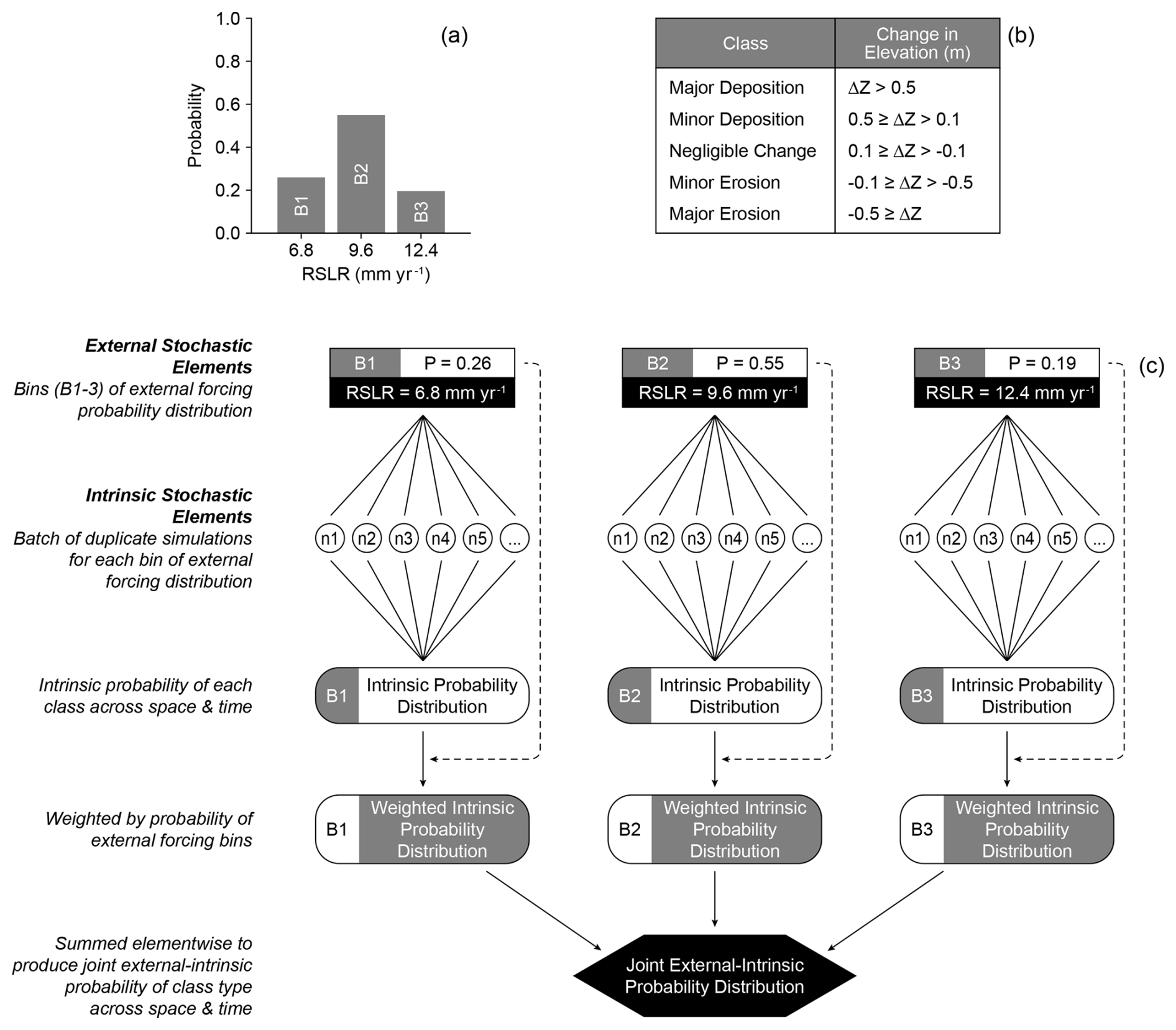
Figure 3Probabilistic model framework. (a) Discrete probability distribution for the rate of RSLR between 2020 and 2050 for North Core Banks, NC, USA, under IPCC SSP5-8.5. (b) Classification scheme for net elevation change used in probabilistic framework examples. (c) Annotated flowchart of the probabilistic framework in MEEB.
For each bin of the external forcing probability distribution, the probabilistic framework in MEEB runs a batch of nP duplicate simulations and determines the class (in this case, the range of elevation change) for each cell in the domain at every timestep for all nP simulations (Fig. 3c). These data are then used to form relative frequency distributions of class type across space and time for the intrinsic stochastic elements. Next, these distributions are weighted (multiplied) by the probability of their external forcing bin. The weighted probability distributions are then summed elementwise to produce a joint external-intrinsic probability distribution of class type for each cell of the model domain across all timesteps (Fig. 3c).
In this work, we use the likelihood of elevation change (relative to the simulation start) as an example of an outcome that can be explored with MEEB. Elevation change is categorized into classes of major deposition, minor deposition, negligible change, minor erosion, and major erosion (Fig. 3b). Other outcomes and categorizations can be developed to suit the goals of the modeling investigation, such as the presence of vegetation or flooding (simple), or ecosystem state (more complex).
Data integration and parameter calibration allows the user to explicitly explore the evolution of a particular setting through time within MEEB. To ensure MEEB best represents a real-world system of interest, thorough data integration and calibration specific to each study location is critical. MEEB integrates empirical data to set initial model conditions and determine the characteristics of the forcing environment. Furthermore, given the myriad process domains, many of which employ poorly constrained parameters, comparison of simulated output to observations is used to both evaluate model performance and, importantly, calibrate process parameter values; similar calibration procedures are typical of microscale models. Scripts for calibrating model parameters and comparing simulated results with observations are included with the model. Data integration and calibration is, of course, dependent on the availability of data, which varies significantly depending upon location and timeframe. Therefore, sources or forms of data different than those described herein can be used as necessary, so long as they are processed to satisfy the same requirements detailed below.
3.1 Case study location
MEEB can theoretically be applied to any sandy barrier system that satisfies the minimal data requirements as described in the following subsections. As a case study, we parameterized and calibrated MEEB for North Core Banks, NC, USA using data from 2014–2018 (National Geodetic Survey, 2024; NCFMP, 2018; USACE NCMP, 2024; USDA Farm Service Agency, 2019; Ritchie et al., 2021; Sturdivant et al., 2019). North Core Banks is a sandy, wave-dominated barrier island 36 km in length, expressing a broad spectrum of ecogeomorphic states from tall, well-developed foredune fields (∼ 5 m above MHW) to frequently inundated overwash flats (Hovenga et al., 2021). Part of the Cape Lookout National Seashore, the barrier is minimally developed and managed to preserve endemic coastal ecosystems and natural ecogeomorphic processes. The regional rate of RSLR from 1994–2024 was approximately 6.3 mm yr−1 (NOAA Tides and Currents, 2024) and dune vegetation is dominated by Ammophila breviligulata, a burial-tolerant dune-building species (Jay et al., 2022).
3.2 Initial conditions
MEEB requires a digital elevation model (DEM) as initial elevation input, paired with contemporaneous spatial rasters of initial vegetation density and species type (Fig. 1a, b). Sufficiently concurrent datasets (<0.5 years apart) ensure that initial vegetation conditions are representative of initial elevation conditions, and vice versa. All elevation and vegetation input raster datasets were resampled to the adopted model grid resolution (here, 1 m) if necessary, clipped to a specified bounding box that defines the spatial domain, and rotated such that the domain axes are parallel with the approximate trend of the barrier shoreline. In order to calibrate model parameter values, a minimum of two sets of observed elevation and vegetation cover datasets are needed to serve as the pre-hindcast initial conditions and the post-hindcast observations for comparison with simulation results. Our methods for satisfying these general data requirements in this case study are described in the following subsections.
3.2.1 Elevation
Initial topobathymetric DEMs were developed from three high-resolution lidar datasets for 2014 (NCFMP, 2018), 2017 (USACE NCMP, 2024), and 2018 (Ritchie et al., 2021). In the absence of bathymetry, and to conform with the model assumption of a linear shoreface geometry, we processed the DEMs by adding the shoreface slope by linearly increasing depth in the cross-shore dimension for all cells seaward of the ocean MHW shoreline according to Ssf,eq. A small back-barrier slope (0.05) was also added by setting the first 30 m landward of the back-barrier MHW shoreline (in the cross-shore dimension) to increase linearly in depth from MHW to Dbb. The back-barrier cells beyond the back-barrier slope are set uniformly to Dbb.
3.2.2 Vegetation
We derived rasters of initial species type from supervised landcover classification datasets for 2014 (Sturdivant et al., 2019) and 2018 (Sara Zeigler and Alexandra Evans, U.S. Geological Survey, unpublished data), generated from orthoimagery captured within the same months as their corresponding elevation datasets. The original landcover datasets were reclassified into three landcover classes: herbaceous vegetation, woody vegetation, and no vegetation. Using the orthoimagery from January to April 2014 (National Geodetic Survey, 2024) and October 2018 (USDA Farm Service Agency, 2019), rough approximations of initial vegetation density for the vegetated classes were derived via the Normalized Difference Vegetation Index, with thresholds set qualitatively for four classes corresponding to ρ values of 0.4, 0.6, 0.8, and 1.0 with random noise perturbations of ±0.1. In qualitatively setting NDVI thresholds, we were able to roughly control for the effect of image seasonality on the NDVI values.
3.3 High-water event climatology
MEEB uses a time series of modeled HWE total water level, duration, and timing for simulation hindcasts. For simulation forecasts, the observed HWE time series serves as the basis for a stochastic HWE environment, which consists of a list of synthetic storms and a probability distribution of storm occurrence based on the time of year, as described in the following.
3.3.1 Hindcast HWE time series
A modeled HWE time series (Fig. 4a) was created using hindcast hourly wave and water level conditions offshore of North Core Banks from 1979 to 2022 (Aretxabaleta et al., 2023), which include significant wave height (Hs), wave period (Tp), water level, and direction. The TWL (i.e., the representative highest elevation of the landward margin of runup) was calculated for each hour as the sum of the maximum 2 % exceedance of wave runup, following Stockdon et al. (2006), and the contemporaneous water-level elevation, which includes tides, storm surge, and other low-frequency fluctuations. Following Wahl et al. (2016) and Reeves et al. (2021), we extracted HWEs from the wave and water-level time series by conditioning upon Hs: HWEs were identified as periods of 8 or more consecutive hours with Hs>2.05 m, which is the minimum monthly averaged wave height for periods in which water levels exceeded the 25th percentile of dune toe elevations (1.78 m NAVD88) at North Core Banks measured from 2005 to 2018 (Doran et al., 2017). If two (or more) periods of 8 or more consecutive hours with Hs>2.05 m occurred less than 24 h apart, the two periods were considered part of the same large-scale weather system and therefore lumped together as single HWE; new HWEs were identified after Hs remained below the 2.05 m threshold for 24 h or longer (Li et al., 2014). Each HWE from the hindcast record is described by its maximum TWL; Hs and Tp concurrent with the maximum TWL; duration; and beginning and ending date/time.
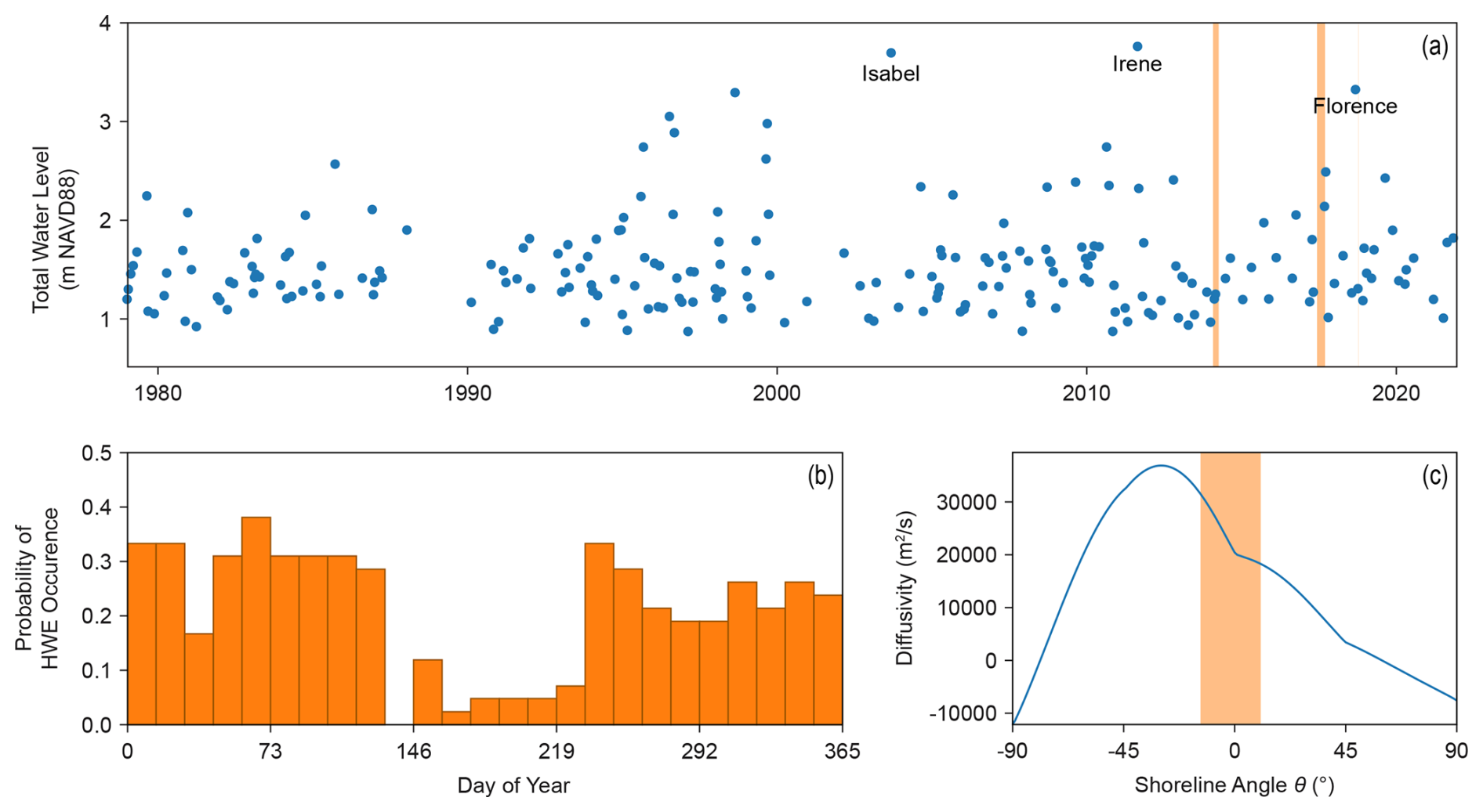
Figure 4Hindcast high water event (HWE) climatology for model input and shoreline diffusivity. (a) Total water level timeseries of HWEs (blue dots) off North Core Banks (NCB), NC, USA from 1979 to 2022; vertical orange bars indicate the dates of capture for the lidar datasets used in this study. Total water level is the sum of tide, surge, and wave runup. (b) Historic (1979–2022) probability of HWE occurrence by time of year; bins are sized according to the Marine component timestep (Δtm=0.04 years). (c) Wave-climate-averaged shoreline diffusivity as a function of shoreline angle θ calculated for a given a, h, Hs, and T representative of NCB; vertical orange bar indicates the range of shoreline angles from the initial 2024 NCB shoreline.
3.3.2 Stochastic HWE environment
The timing and characteristics (TWL and duration) of HWEs are determined stochastically in model forecasts. For each Marine iteration in the model (Δtm=0.04 years), a HWE may occur based upon the historical probability of HWE occurrence for each iteration in the observed HWE record, which was calculated as the number of years in which one or more HWEs occurred during each Marine timestep divided by the total length (in years) of the observational record (Fig. 4b). If a HWE is determined to occur, the TWL and duration is chosen from a list of 10 000 synthetic HWEs generated using the copula-based, multivariate sea-storm model from Wahl et al. (2016), which identifies interdependencies among relevant sea-storm parameters (water level, Hs, Tp, and duration) using the observed HWE record as required input. MEEB assumes that the probability of HWE occurrence for each iteration, as well as the characteristics of the synthetic HWEs (i.e., the average TWL and duration of the 10 000 synthetic HWEs), remain constant over the course of a simulation.
3.4 Wave climatology
MEEB requires estimates for long-term (multidecadal) averaged wave climate characteristics to drive alongshore shoreline diffusion, as described in Sect. 2.4.2. We used the same hindcast hourly wave and water-level conditions offshore of North Core Banks from 1979 to 2022 (Aretxabaleta et al., 2023) to derive the mean offshore significant wave height, mean wave period, and the wave climate asymmetry and proportion of high-angle waves (relative to the barrier shoreline trend) for the time period, which allows for computation of multidecadal shoreline change.
3.5 Probabilistic distribution of future RSLR
We developed a probabilistic distribution of RSLR for the year 2050 (Fig. 3a) from the IPCC AR6 SSP5-8.5 sea-level projections (Fox-Kemper et al., 2021; data available from Garner et al., 2021) for the grid tile encompassing North Core Banks at 34° N 77° W. Following others (Wainwright et al., 2015; Bamunawala et al., 2021), a triangular probability distribution of RSLR was created using the 5, 50, and 95 quantiles of the projected RSLR for the year 2050 under SSP5-8.5. This triangular distribution was then transformed into a discrete probability distribution with three bins.
SSP5-8.5 represents a “very high” greenhouse gas emissions pathway, and the accompanying sea-level rise projection follows a trajectory most similar to the NOAA “Intermediate” scenario from Sweet et al. (2022). Users can run the same probabilistic model framework with different RSLR probability distributions representative of other SSPs, and the results of multiple pathways can thereby be compared. For example, users can select and make projections for two pathways that correspond to “most likely” and “worst case” scenarios. For the year 2050, however, there is relatively little difference in projected sea levels between the highest and lowest IPCC SSPs, with considerable overlap of ranges. The relative convergence of RSLR to greenhouse gas emissions over the next three decades suggests a single SSP for a “very high” emissions pathway (i.e., SSP5-8.5) is sufficient for probabilistic projections up to the year 2050, in alignment with findings from the 2022 NOAA Interagency Technical Report for sea-level rise (Sweet et al., 2022).
3.6 Skill assessment and parameter optimization
We define model performance primarily through the direct cell-by-cell comparison of simulated and observed elevation with the Brier Skill Score (BSS), which measures how much the simulated change improves a prediction relative to the baseline of predicting no change at all:
where J is the total number of cells in the skill determination, simj is the simulated final elevation at cell j, obsj is the observed final elevation at cell j, and bj is the baseline prediction equal to the initial elevation at cell j (i.e., assumes no change). When specifically assessing the aeolian performance of the model, we also determined the BSS of the change in foredune crest elevation. While our skill assessment used a conventional cell-by-cell, point-based approach, future model calibration may benefit from alternative metrics that capture more qualitative behaviors or states (French et al., 2016; Murray, 2003).
We used particle swarm optimization (PSO) to calibrate 15 free parameters to maximize model skill. PSO is a metaheuristic computational method to search iteratively for the global optimum within a given parameter space. PSO seeds the parameter space with particles (i.e., specific sets of parameter values) that make up a swarm (i.e., a population of candidate solutions). The movement of each particle is guided both by its own local best-known position within the parameter space as well as the best-known position of the entire swarm. Over many iterations, the swarm tends to descend upon the global optimum set of parameter values that maximizes the model skill, while tending to avoid local optima. A minimum and maximum value for each parameter defines the calibration space; see Table A1 in the Appendix for the range of values used for each calibrated free parameter.
We optimized Aeolian and Marine parameters separately to reduce the number of free parameters calibrated at once and improve potential calibration. First, Marine parameters alone were optimized using only the Marine component of MEEB over a single HWE event: Hurricane Florence, which made landfall as a Category 1 hurricane in September 2018 south of Wrightsville Beach, NC, USA, was used for Marine calibration because of extensive overwash on North Core Banks and the availability of lidar captured 3 weeks after the event (Ritchie et al., 2021). We used a skill score for change in elevation that was designed to be representative of the barrier as a whole, calculated as the average BSS of elevation change across five ecogeomorphologically diverse, 300 m-long training sites characterized by a small and large overwash fan, a small and large overwash flat, and a tall continuous dune ridge (Figs. 5, 6). To best ensure that the observed change is representative of HWE impacts, determination of skill was limited to subaerial cells that fall seaward of the dune crest or within either the simulated or observed overwash extent. Observed overwash extent was digitized by hand with pre- (June to September 2017; USACE NCMP, 2024) and post-Florence (October 2018; Ritchie et al., 2021) imagery and lidar as reference.
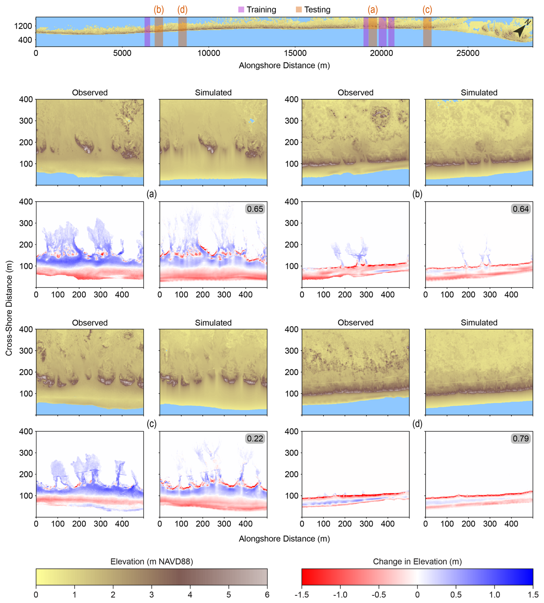
Figure 5Hindcast simulations testing performance of the MEEB Marine component with calibrated Marine parameters. (a–d) Observed and simulated post-Florence elevation and pre- to post-Florence elevation change at 4 test locations across North Core Banks, NC, USA. Locations of each marine testing site, as well as each marine training site used in calibration, are indicated in the top map. The Brier Skill Score for each hindcast (a–d) is given in the gray boxes and Table 1.
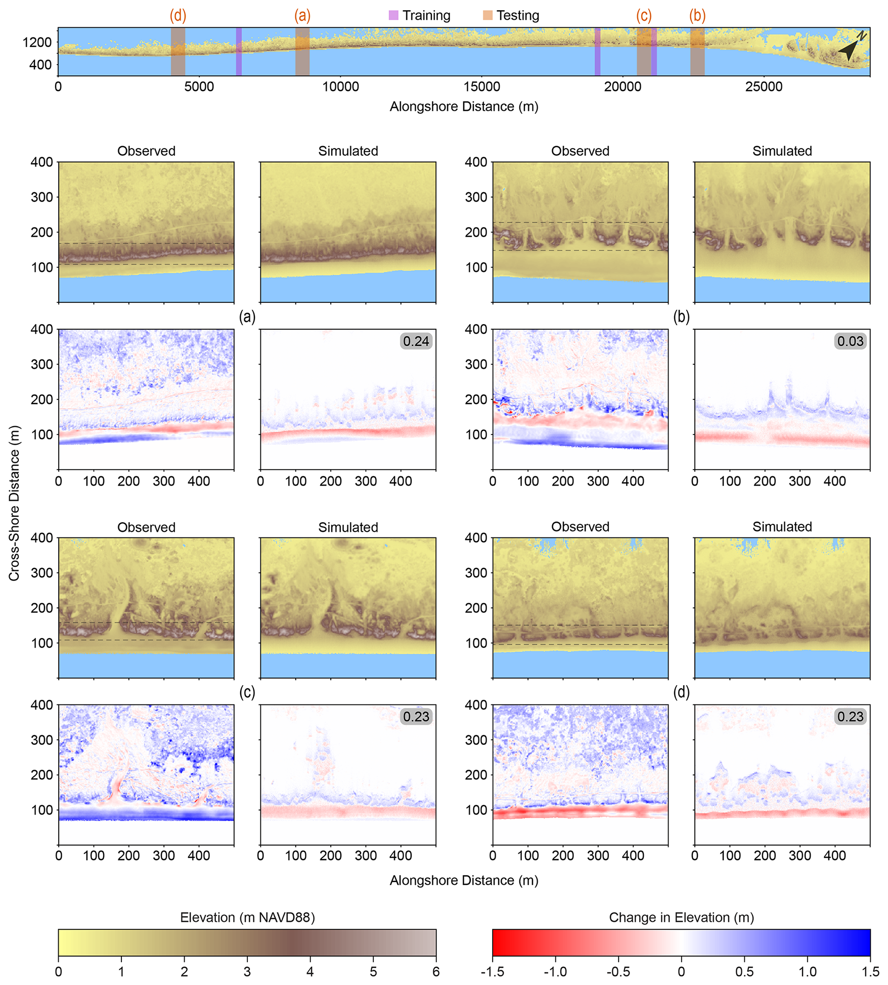
Figure 6Hindcast simulations (for the period of April 2014 to September 2017) testing MEEB performance with calibrated Aeolian parameters. (a–d) Observed and simulated post-simulation elevation and pre- to post-simulation elevation change at 4 test locations across North Core Banks, NC, USA. Locations of each aeolian testing site, as well as each aeolian training site used in calibration, are indicated in the top map. The Brier Skill Score for each hindcast (a–d) is given in the gray boxes and Table 1. Skill determination is confined to the area between the dashed lines at each location to focus calibration on foredune growth and exclude error in the lidar DEMs associated with reflectance off the vegetation surface. Areas of apparent significant accretion landward of the foredune field in (a)–(d) are artefacts of the post-Florence lidar capturing the shrub canopy elevations versus the true surface elevation in the pre-Florence lidar.
Next, Aeolian parameters were optimized by running the model over a period of relatively limited HWE activity (16 April 2014 to 16 September 2017), thereby controlling for the effects of marine processes on the Aeolian calibration. Results from the preceding Marine parameter calibration were used to set the Marine parameter values for the Aeolian calibration, and all components of MEEB (Aeolian, Marine, Shoreline, and Vegetation) were utilized and active. The RSLR rate was set to 6 mm yr−1 for these hindcasts, representative of historical conditions. We used a multi-objective skill score calculated as the average of the BSS for cell-by-cell elevation change and the BSS for dune crest height change. Including dune height as part of the multi-objective skill score helps prioritize accurate representation of vertical foredune growth over other characteristics, particularly as foredune height has a large impact on barrier response to HWEs. To focus calibration on foredune growth and to exclude interior areas with error in the lidar DEMs associated with reflectance off the vegetation surface, determination of skill was also limited to cells within a specified foredune field (Fig. 6). This multi-objective score was averaged again across three diverse, 200 m-long training sites to produce a single score representative for North Core Banks as a whole. To calibrate the four wind-direction probabilities (PWD) that collectively sum to 1, we used three parameters that can be tuned independently from each other: (1) the wind axis ratio, which is the ratio of wind directed cross-shore relative to alongshore; (2) the onshore wind ratio, which is the ratio of cross-shore wind directed onshore relative to offshore; and (3) the down-shore wind ratio, which is the ratio of alongshore wind directed down the coastline relative to up. The four values of PWD were calculated from the three resulting calibrated wind parameters. While historical wind direction data from North Core Banks is available for input into MEEB, we found calibrating the wind direction probabilities directly produced significantly better agreement with observations. This may be because the dominant historical wind directions at North Core Banks run oblique to the shoreline and therefore our model grid orientation, coupled with the fact that aeolian transport in the model is constricted to directions directly parallel with model gridlines (i.e., not diagonal), suggesting limitations to the relatively simple aeolian algorithm employed in MEEB (see also Nield and Baas, 2008a). Future research into incorporating wind direction observations, particularly with oblique wind directions, could prove fruitful.
Due to challenges in generating effective skill scores for hindcasts of vegetation cover, we did not calibrate Vegetation free parameters; instead, Vegetation parameter values roughly follow those of Nield and Baas (2008a) and Keijsers et al. (2016). Shoreline parameters, with perhaps the exception of the alongshore sediment transport constant kd, can be directly estimated and therefore do not necessitate optimization.
3.7 Sensitivity analyses
We investigated the global sensitivity of model output to input parameter variations for the purpose of ranking variables according to their relative contribution to output variability and screening variables that have minimal effect on output variability. We used the Method of Morris test (Morris, 1991), also known as the Elementary Effects Test, which is well-suited for models like MEEB with numerous input variables and/or relatively long run times (Pianosi et al., 2016). The Method of Morris determines both the overall importance of a parameter (μ∗; the mean of the absolute value of the elementary effects) and its degree of interaction with other input parameters (σ∗; the standard deviation of the absolute value of the elementary effects). As in the calibration workflow, we performed sensitivity analyses on the Aeolian and Marine components of the model separately, and used the same experimental setup, skill scores, and input parameter ranges. Because the Method of Morris depends on the range of input parameter values and because several parameters in MEEB are poorly constrained and abstract, conclusions drawn from our sensitivity analyses are relevant only with regards to the estimated ranges of parameter values used herein (Table A1). Our sampling strategy used six grid levels (which controls the sampling grid and variation sizes; Morris, 1991; Pianosi et al., 2016), with 75 aeolian and 115 marine trajectories resulting in 900 and 1150 combinations of parameter values evaluated for the Aeolian and Marine components of the model, respectively.
4.1 Parameter sensitivity analyses
Our parameter sensitivity analyses suggest that the Marine component of MEEB is most sensitive to the erosive timescale calibration coefficient (Te) and equilibrium beach slope (βeq), followed by the overwash infiltration and drag parameter (Rd) and sediment transport coefficients (Kow, m; Fig. 7a). These parameters also display the highest degree of interaction with each other (Fig. 7a). The Marine component in MEEB is insensitive to the vegetation flow-reduction coefficient (Λ), which controls the degree to which vegetation impacts the overwash flow, for both types of vegetation; we therefore did not include these parameters in our final calibration. Perhaps unsurprisingly, marine evolution in the model is particularly sensitive to poorly constrained coefficients (Te, Kow, m) that have limited relevance to real-world measurements or observations. That overwash in the model is particularly sensitive to infiltration and drag of the flow across the barrier interior (Rd) suggests continued study and measurement of these factors across the barrier landscape could be especially beneficial.
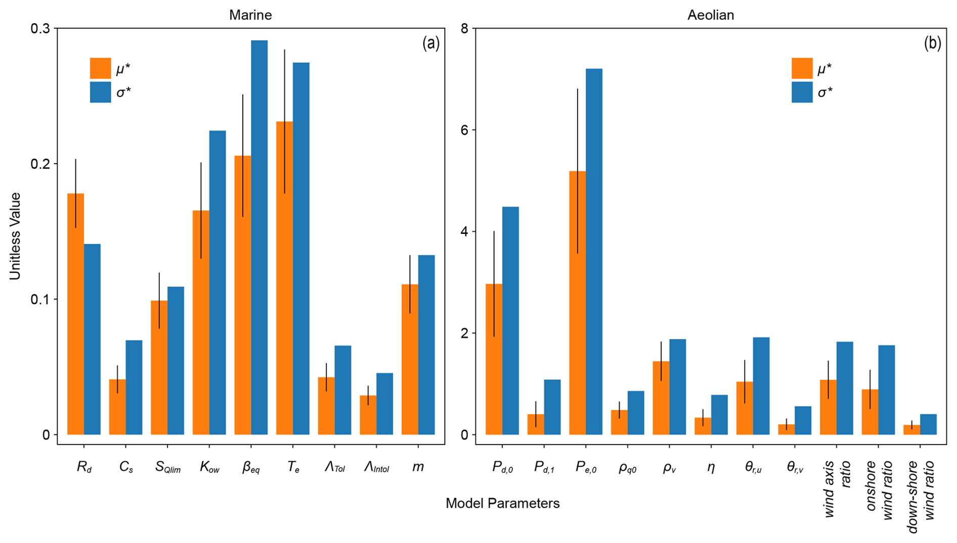
Figure 7Sensitivity analyses of model parameters for the (a) Marine and (b) Aeolian model components. Marine and Aeolian parameters are analyzed separately following the same design and parameter ranges as the parameter calibration simulations. Unitless values for the overall importance of a parameter (μ∗) and its degree of interaction with other parameters (σ∗) are given in orange and blue, respectively. Black lines represent the 95 % confidence interval.
The Aeolian component of MEEB is most sensitive, by far, to the probabilities of deposition (Pd,0) and erosion (Pe,0) in the absence of vegetation (Fig. 7b). These parameters also display the highest degree of interaction with other parameters. The model is insensitive to both the unvegetated and vegetated angles of repose (θr,u, θr,v), and we therefore exclude them from the model optimization. Overall, aeolian evolution in the model is most sensitive to parameters controlling the volumetric sediment flux, as opposed to the exact specifications of the way in which vegetation density and type alter this flux.
4.2 Hindcasts: comparisons to observations
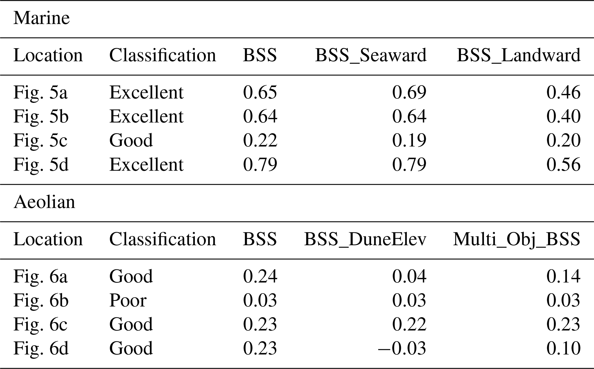
To assess model skill, we ran hindcast simulations using the calibrated parameter values and the same simulation set-up as in calibration except at testing sites that differ from the training sites (Figs. 5, 6). Simulation results were compared to observed elevation change and the resulting model skill scores are given in Table 1. Our testing sites each span 0.5 km in length alongshore to demonstrate the variability of model performance in different geomorphic settings; with increasingly larger model domain extents, the skill scores would tend to approach the mean score of the entire barrier.
Table 1Model skill scores for elevation change from MEEB hindcast simulations. BSS = cell-by-cell Brier Skill Score; BSS_Seaward = BSS of all cells seaward of the post-storm foredune crest; BSS_Landward = BSS of all cells landward of the post-storm foredune crest; BSS_DuneElev = BSS of change in elevation of all foredune crest cells; Multi_Obj_BSS = average of BSS and BSS_DuneElev. Brier Skill Score qualitative classification follows Sutherland et al. (2004).
Hindcast simulations of Hurricane Florence using calibrated Marine parameters produce good to excellent agreement with observations (following the BSS categorization from Sutherland et al., 2004) for pre- to post-storm elevation change at four test sites across North Core Banks (Fig. 5; Table 1). Good to excellent agreement is also found when considering elevation change landward of the foredune crest in isolation, as well as fair to excellent agreement seaward of the foredune crest (Table 1). MEEB does particularly well in capturing overwash deposition patterns and washover thicknesses. Naturally, the model is more skillful at some test sites across the barrier than others. In particular, the model tends to overestimate dune scarping in certain areas, particularly where overwash flows through gaps in the foredune line (Fig. 5a, c). MEEB also tends to underestimate lateral spreading of overwash flow in areas with confined or channelized topography (Fig. 5b), a direct consequence of the simplified flow-routing algorithm that directs flow only to the three landward neighboring cells.
Testing the skill of calibrated Aeolian parameters, hindcast simulations from April 2014 to September 2017 (a period of minimal storm activity) at four test sites across North Core Banks result in good to poor agreement with observed topographic change (Fig. 6; Table 1). As in calibration, the skill assessment was applied only to cells within the predetermined dune field (Fig. 6). While beach change is predicted poorly in some of the hindcasts (Fig. 6b, c), it is beyond the intent of the model to predict fluctuations in beach state on a monthly or seasonal timescale. Importantly, the model appears to do qualitatively well in capturing the location and/or pattern of dune growth. This includes the one hindcast with a poor (0.04) BSS (Fig. 6b), suggesting that our simple multi-objective BSS could be improved to better identify and prioritize important qualitatively correct behaviors (French et al., 2016) and better align with subjective judgements of similarity (Bosboom and Reniers, 2014). In our tests, the model tends to underestimate the vertical extent of dune growth. Additionally, aeolian reworking of the barrier interior (landward of the foredune crest) is overestimated in some areas (Fig. 6a, d), suggesting that the model is sensitive to the initial vegetation conditions.
4.3 Forecasts: probability of future change
MEEB was developed to provide useful projections at spatiotemporal scales relevant to coastal management. Here, the model is exercised in a predictive application using the probabilistic framework described in Sect. 2.6 and the RSLR probability distribution described in Sect. 3.5. We run example probabilistic projections of elevation change for the year 2050 at an initially overwash-prone site and an initially overwash-resistant site on North Core Banks. While these sites span only 0.5 km in length alongshore for the purpose of providing a clear and concise demonstration of model output, MEEB can handle model domains up to tens of kilometers in alongshore length. Figure 8 plots the most likely range of net elevation change across the model domain from 2018 to 2050 for these projections. At the initially overwash-prone site (Fig. 8a–c), the model projection suggests that major deposition is most likely at the proximal parts of the overwash fans with minor deposition most likely on the more distal portions (Fig. 8b). Repeated overwash events will tend to prevent vegetation from recolonizing the overwash fans over the course of the simulation. Consequentially, aeolian deflation of the sparsely vegetated overwash fans, and resulting minor deposition along the landward vegetated fringes of the fans (cf. Rodriguez et al., 2013), is also predicted to be likely. The model also predicts the high likelihood of major accretion around the seaward slope and toe of the present foredunes, reflecting the steeping of the beach profile with net seaward growth of the foredune system and likely net seaward expansion of vegetation cover. This probabilistic projection suggests that the areas encompassing the washover fans are likely to remain vulnerable to persistent overwash through the year 2050, while foredune areas are likely to not only be stable but expand.
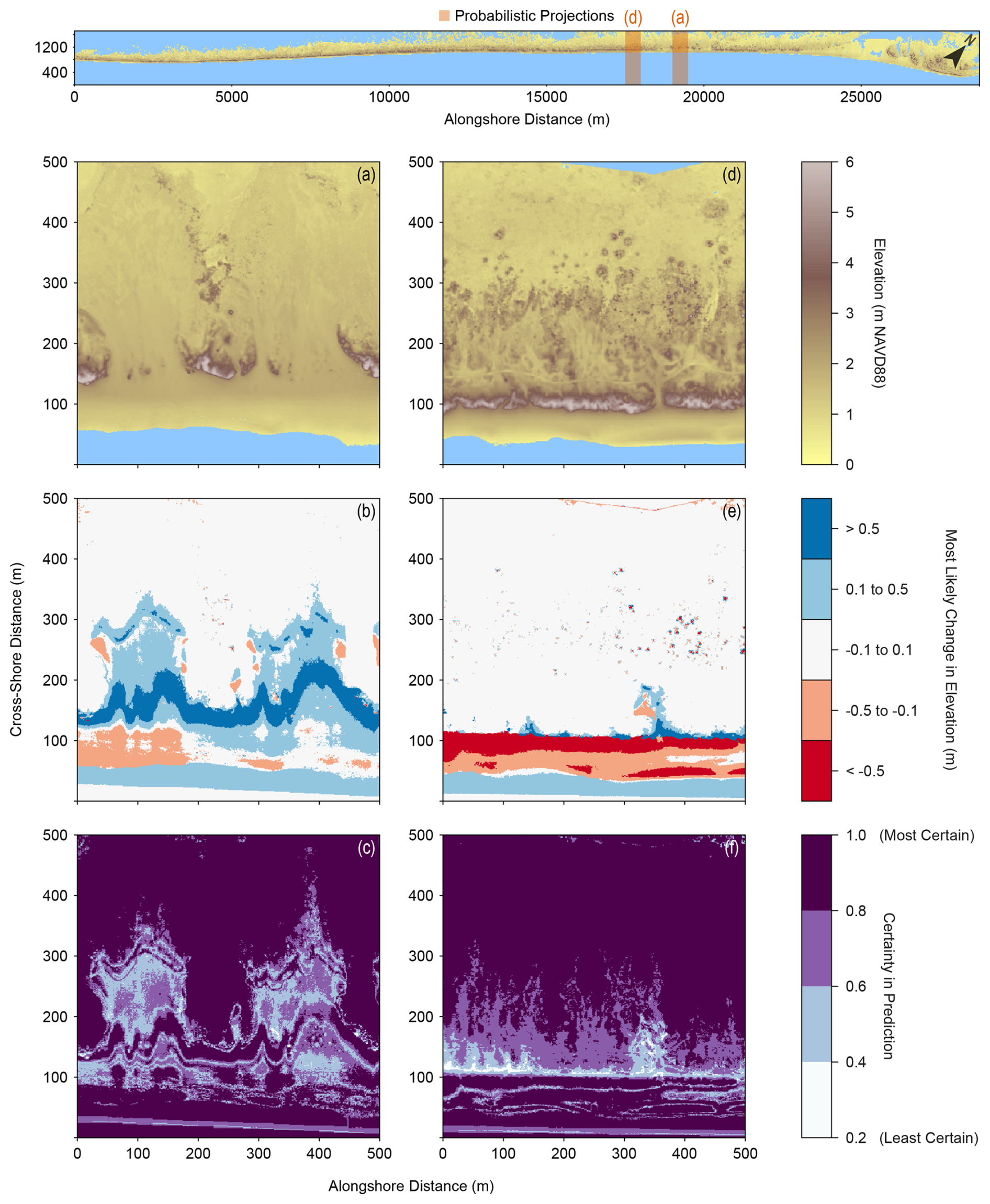
Figure 8Example probabilistic projections of elevation change for the year 2050, at two sites on North Core Banks, NC, USA: (a–c) an initially overwash-prone site and (d–f) an initially overwash-resistant site. Locations of both sites are indicated in the top map. (a, d) Initial 2018 topography for the overwash-prone and overwash-resistant sites, respectively. (b, e) Most likely net change in elevation between 2018 and 2050 classified into five elevation ranges. (c, f) Certainty in most likely elevation change predictions, taken as the proportion of all model runs resulting in the most likely class of elevation change.
At the initially overwash-resistant site (Fig. 8d–f), the probabilistic projection suggests that major lateral dune erosion via scarping is likely to occur but that the foredune ridge will most likely persist (Fig. 8e). Aeolian deposition near the initial foredune crest is likely to offset some of the height and volume lost from dune scarping. As a result of this persistent and resistant topography, dense vegetation will tend to cover the barrier interior and prevent aeolian reworking landward of the dune crest. Although the model predicts negligible elevation change is most likely landward of the foredune crest, uncertainty in this prediction – particularly near the left (Southwest) edge of the model domain – reflects the small but very real possibility of minor to major overwash deposition in the event of foredune overtopping and/or loss (Fig. 8f). Overall, this projection indicates that vulnerability to HWE-driven change is low through 2050 landward of the initial 2018 foredune crest, though the high probability of major dune width loss in this period suggests that the likelihood of a shift in morphologic regime from overwash-resistant to overwash-prone may increase rapidly in the subsequent decades. Potential increases in future HWE intensity (e.g., Knutson et al., 2020) could also enhance the likelihood of more fundamental morphological and ecological regime changes by 2050 – such fundamental changes would also be likely to occur by the end of the century.
MEEB was developed to simulate spatially explicit, ecogeomorphic, probabilistic evolution of coastal barrier systems over spatiotemporal scales of greatest interest to coastal managers and decision-makers. The goal of the model is to reconcile management needs for projections that are both quantitative/place-specific and multi-decadal/multi-kilometer (i.e., mesoscale) while accounting for ecogeomorphic feedbacks and uncertainties in the forces driving future change. In our approach for modeling mesoscale barrier ecogeomorphic evolution, we (a) integrated model parameterizations of varying mechanistic complexity, representing certain processes or interactions with relatively higher complexity (only as far as needed to produce mesoscale behaviors anticipated to be important) within an otherwise synthesist framework, and (b) thoroughly tested and calibrated these parameterizations with observational data. Because many of these relatively simple and heuristic algorithms involve calibration coefficients and poorly constrained independent variables, we have made a substantial effort to determine which of these parameters are most influential to model outcomes and assign values that provide the best model agreement with observations, as evaluated by our multi-objective skill scores for hindcasts on North Core Banks. While the model has yet to be applied to other sites, North Core Banks is an ideal case study location given its relative lack of human influence, multiple ecosystem types and barrier states, history of ecogeomorphic change, and availability of high-quality data, and therefore may be representative of other undeveloped barrier environments. Given the demonstrated skill of our hindcasts of North Core Banks, as well as our holistic and simplistic model representations of ecogeomorphic processes and interactions, we expect MEEB to be widely adaptable to most minimally-engineered barrier systems along the U.S. East and Gulf coasts. The model may be less applicable to barrier environments strongly influenced by tidal inlet dynamics, complex shoreline change, or human management, though in the future a human management module could be added to MEEB (e.g., Anarde et al., 2024a, b) to explore the ecogeomorphic effects of coupled human–natural interactions.
As with any numerical model, appropriate interpretation of the results depends on the scale and complexity of the model parameterizations. As a mesoscale model, MEEB is not suitable for investigations with the goal of predicting subtle changes in elevation or vegetation cover; nor is it an appropriate tool for explaining the large-scale behaviors of landscape configuration, such as the drowning of a barrier chain. Instead, MEEB is designed to answer questions about barrier ecogeomorphic change of moderate complexity by offering semi-qualitative predictions and semi-quantitative explanations. For example, MEEB can be used to investigate the effects of climate-induced shifts in ecological composition by adjusting Vegetation parameters over time to represent transitions in vegetation assemblages. Such transitions could affect the likelihood of coastal hazard impacts by altering aeolian growth rates and/or patterns and therefore landscape vulnerability to HWEs. As another example application, MEEB could be used to predict where and when overwash along a barrier is most likely to occur by generating probabilistic projections of overwash inundation through time and identifying ecogeomorphic indicators of overwash vulnerability. Future work could compare MEEB simulations with micro- (e.g., XBeach, Roelvink et al., 2009) or macro-scale (e.g. LTA14, Lorenzo-Trueba and Ashton, 2014) models to explicitly determine when, where, and how the trajectories of the models overlap in their respective utility.
To simulate spatially explicit ecological and geomorphological processes across an entire subaerial barrier landscape over several decades, MEEB employs many synthesized parameterizations and simplifying assumptions. Inevitably, MEEB bears several important limitations arising from this modeling approach. For example, MEEB assumes the barrier system is composed entirely of unconsolidated sand, whereas grain sizes and characteristics can vary over meters to kilometers in ways that affect dune growth (e.g., Hovenga et al., 2023) and barrier transgression (e.g., Brenner et al., 2015). Tidal inlet and breaching processes, including outwash events (Sherwood et al., 2023), are neglected in MEEB, despite the significant ecomorphodynamic changes associated with these processes and their importance to long-term transgressive sediment flux (e.g., Nienhuis and Lorenzo-Trueba, 2019b; Leatherman, 1979; Passeri et al., 2020; Sherwood et al., 2023). Therefore, we exclude portions of a barrier within several hundred meters of active tidal inlets and breaches from the model domain, rendering the model less relevant to tide-dominated barrier systems where barriers are frequently segmented by inlet channels. Further, MEEB models the long-term, wave-climate-averaged shoreline diffusivity by assuming the diffusive wave climate does not change over the course of a simulation, which may average over variability in shoreline diffusion that could potentially feedback with coupled ecogeomorphic processes (e.g., dune erosion). MEEB also presently assumes that no shoreline changes resulting from alongshore transport gradients occur at the domain boundaries (i.e., shoreline change at these cells only occurs from cross-shore processes). As such, if the MEEB model domain were part of a curved coastline eroding or accreting due to persistent alongshore transport gradients (Ashton and Murray, 2006), local shoreline change rates would be underpredicted. Lastly, the Vegetation component presently lacks finer temporal resolution needed to capture seasonal variations in vegetation density and growth, which could play an important role in how a barrier responds to and recovers from HWEs. Additionally, the simplified Vegetation component lacks many of the environmental filters (e.g., temperature, groundwater depth, elevation, salinity) that could affect the zonation and density of vegetation, with implications for aeolian and overwash sediment transport and thereby projections of future change. To improve the utility of MEEB for addressing the ecogeomorphic effects of climate-induced shifts in ecology, the model would require the addition of seasonality and species zonation dynamics.
Despite these limitations, comparisons of MEEB hindcast simulations to observations demonstrate that our relatively simple set of parameterizations for coupled aeolian, marine, vegetation, and shoreline processes can skillfully capture important mesoscale dynamics of barrier systems. This is achieved in large part through thorough calibration of the most sensitive free parameters, with integration of topographic, ecologic, and storm climatology data to set initial conditions and assess model performance. A single set of calibrated parameter values performs well at ecogeomorphologically diverse test sites spread across the nearly 30 km domain and in hindcast simulations spanning multiple continuous years, leading to confidence in model projections of future mesoscale change.
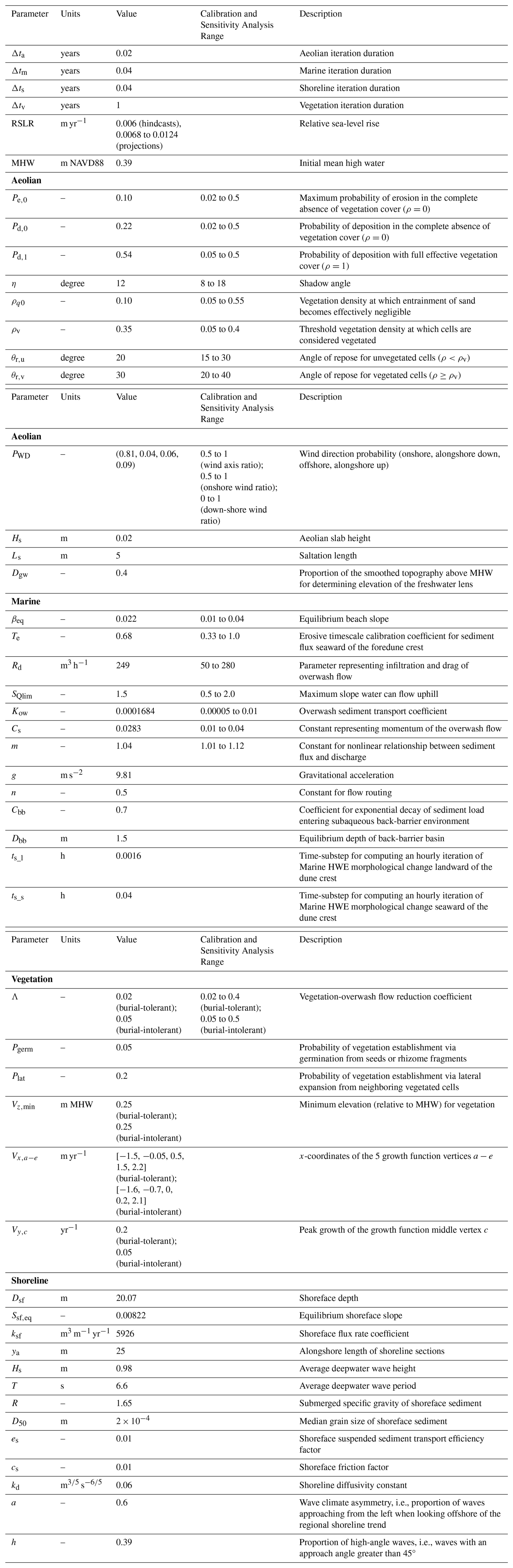
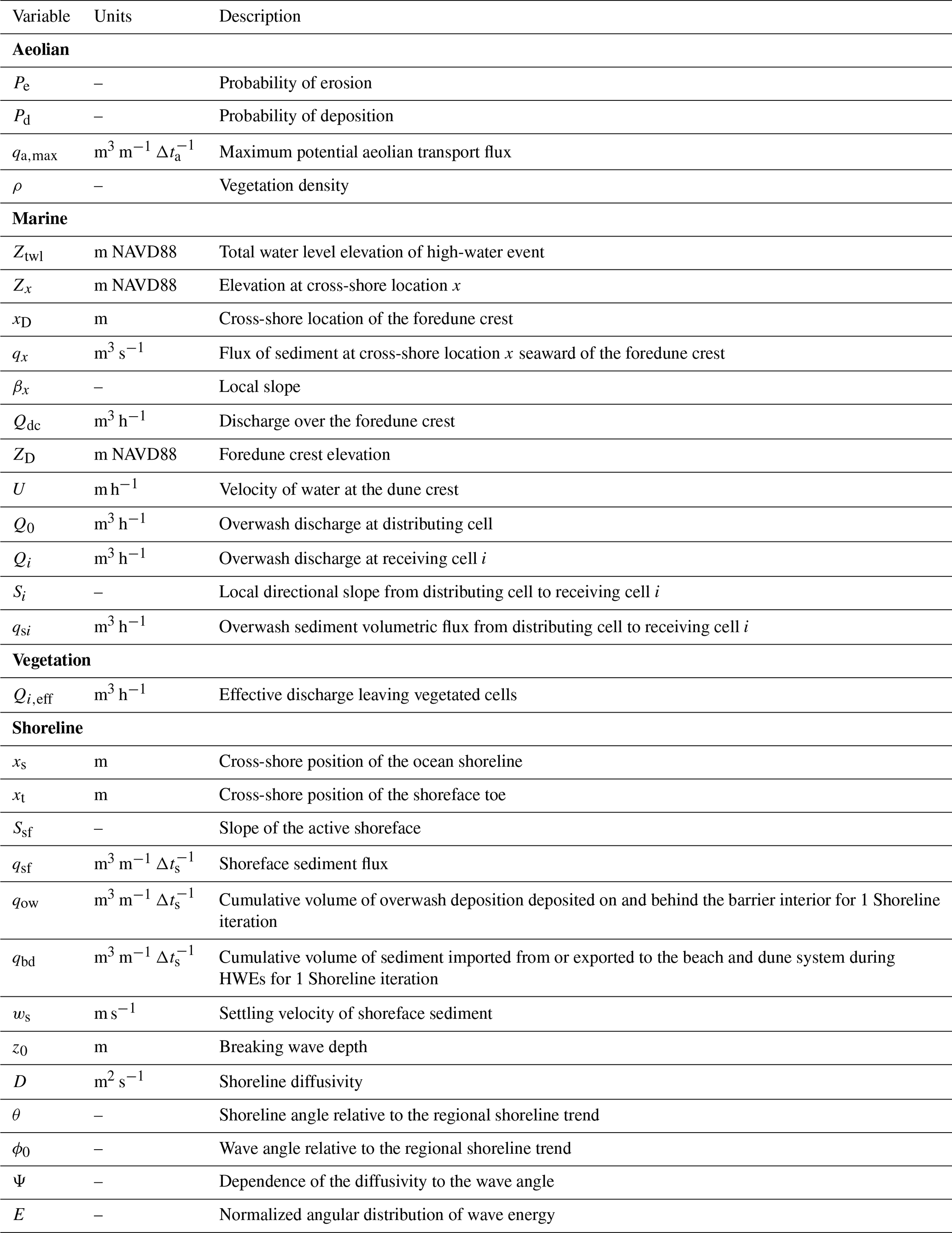
MEEB v1.0 source code and documentation are available at https://doi.org/10.5066/P13N6RHA (Reeves, 2025a), the official USGS software release, under a CC0 1.0 Universal license. A public copy of the MEEB v1.0 code and documentation is also archived on Zenodo at https://doi.org/10.5281/zenodo.15014191 (Reeves, 2025b). All elevation and vegetation input files used in the calibration procedures and simulations presented in this work are stored within the archived MEEB v1.0 software release (Reeves, 2025a, b) at /MEEB/Input. Hindcast hourly wave and water level conditions offshore of North Core Banks from 1979 to 2022, used to develop the observed HWE timeseries and stochastic HWE environment, are available from the Renaissance Computing Institute (https://renci.github.io/edsreanalysisdoc/, Blanton et al., 2024) and stored within the MEEB v1.0 software release at /MEEB/Data/NorthCoreBanks.
IRBR developed the model code, prepared input data, ran the simulations, analyzed the results, and wrote the original draft of the manuscript. All authors contributed to the project conceptualization, methodology, and editing of the manuscript.
The contact author has declared that none of the authors has any competing interests.
Any use of trade, firm, or product names is for descriptive purposes only and does not imply endorsement by the U.S. Government.
Publisher's note: Copernicus Publications remains neutral with regard to jurisdictional claims made in the text, published maps, institutional affiliations, or any other geographical representation in this paper. While Copernicus Publications makes every effort to include appropriate place names, the final responsibility lies with the authors. Views expressed in the text are those of the authors and do not necessarily reflect the views of the publisher.
This work was supported by a Woods Hole Oceanographic Institution and U.S. Geological Survey Postdoctoral Scholar Fellowship, and the U.S. Geological Survey Coastal and Marine Hazards and Resources Program as part of the Remote Sensing Coastal Change and Future Landscape Adaptation and Coastal Change projects. IRBR was supported in part by the U.S. Geological Survey's John Wesley Powell Center for Analysis and Synthesis as part of a working group entitled “Beyond waves and shifting sand: considering ecosystem processes in forecasts of coastal ecosystem change”; this project was co-sponsored by the National Science Foundation under grant 23DEB10330. Wave and water-level model hindcasts used in this work were provided by the Renaissance Computing Institute. The authors thank reviewers Eli Lazarus and Andy Wickert for providing thoughtful comments that helped to significantly improve this manuscript.
This research has been supported by the National Science Foundation (grant no. 23DEB10330).
This paper was edited by Andy Wickert and reviewed by Eli D. Lazarus and Andy Wickert.
Anarde, K. A., Moore, L. J., Murray, A. B., and Reeves, I. R. B.: The future of developed barrier systems: 2. Alongshore complexities and emergent climate change dynamics, Earth's Future, 12, e2023EF004200, https://doi.org/10.1029/2023EF004200, 2024a.
Anarde, K. A., Moore, L. J., Murray, A. B., and Reeves, I. R. B.: The future of developed barrier systems: 1. Pathways toward uninhabitability, drowning, and rebound, Earth's Future, 12, e2023EF003672, https://doi.org/10.1029/2023EF003672, 2024b.
Aretxabaleta, A. L., Sherwood, C. R., Blanton, B. O., Over, J.-S. R., Traykovski, P. A., and Sogut, E.: Temporal variability of runup and total water level on Cape Cod sandy beaches, in: The Proceedings of the Coastal Sediments 2023, Coastal Sediments 2023, New Orleans, LA, USA, 267–281, https://doi.org/10.1142/9789811275135_0024, 2023.
Ashton, A. D. and Murray, A. B.: High-angle wave instability and emergent shoreline shapes: 1. Modeling of sand waves, flying spits, and capes, Journal of Geophysical Research: Earth Surface, 111, https://doi.org/10.1029/2005JF000422, 2006.
Baas, A. C. W.: Chaos, fractals and self-organization in coastal geomorphology: Simulating dune landscapes in vegetated environments, Geomorphology, 48, 309–328, https://doi.org/10.1016/S0169-555X(02)00187-3, 2002.
Baas, A. C. W. and Nield, J. M.: Modelling vegetated dune landscapes, Geophysical Research Letters, 34, L06405, https://doi.org/10.1029/2006GL029152, 2007.
Bamunawala, J., van der Spek, A., Dastgheib, A., Murray, A. B., and Ranasinghe, R.: An integrated, probabilistic modeling approach to assess the evolution of barrier-island systems over the twenty-first century, Frontiers in Marine Science, 8, 755699, https://doi.org/10.3389/fmars.2021.755699, 2021.
Blanton, B. O., McManus, J. M., and Tilson, J. L.: Accessing the RENCI/NOAA Reanalysis datasets V2.00, Renaissance Computing Institute, https://renci.github.io/edsreanalysisdoc/ (last access: 10 June 2024), 2024.
Bosboom, J. and Reniers, A. J. H. M.: Displacement-based error metrics for morphodynamic models, Adv. Geosci., 39, 37–43, https://doi.org/10.5194/adgeo-39-37-2014, 2014.
Brenner, O. T., Moore, L. J., and Murray, A. B.: The complex influences of back-barrier deposition, substrate slope and underlying stratigraphy in barrier island response to sea-level rise: Insights from the Virginia Barrier Islands, Mid-Atlantic Bight, U.S.A., Geomorphology, 246, 334–350, https://doi.org/10.1016/j.geomorph.2015.06.014, 2015.
Bruun, P.: Sea-level rise as a cause of shore erosion, Journal of the Waterways and Harbors Division, 88, 117–130, https://doi.org/10.1061/JWHEAU.0000252, 1962.
Durán Vinent, O. and Moore, L. J.: Barrier island bistability induced by biophysical interactions, Nature Climate Change, 5, 158–162, https://doi.org/10.1038/nclimate2474, 2015.
Doran, K. S., Long, J. W., Birchler, J. J., Brenner, O. T., Hardy, M. W., Morgan, K. L. M., Stockdon, H. F., and Loubriel Torres, M.: Lidar-derived beach morphology (dune crest, dune toe, and shoreline) for U.S. sandy coastlines, version 5.0, U.S. Geological Survey [data set], https://doi.org/10.5066/F7GF0S0Z, 2017.
FEMA: Guidance for Flood Risk Analysis and Mapping, Coastal Statistical Simulation Methods, Federal Emergency Management Agency, Washington, D.C., 36 pp., https://www.fema.gov/sites/default/files/documents/Coastal_Statistical_Simulation_Methods_Nov_2023.pdf (last access: 12 June 2024), 2023.
Ferguson, R. I. and Church, M.: A Simple Universal Equation for Grain Settling Velocity, Journal of Sedimentary Research, 74, 933–937, https://doi.org/10.1306/051204740933, 2004.
Fox-Kemper, B., Hewitt, H. T., Xiao, C., Aðalgeirsdóttir, G., Drijfhout, S. S., Edwards, T. L., Golledge, N. R., Hemer, M., Kopp, R. E., Krinner, G., Mix, A., Notz, D., Nowicki, S., Nurhati, I. S., Ruiz, L., Sallée, J.-B., Slangen, A. B. A., and Yu, Y.: Ocean, cryosphere and sea level change, in: Climate Change 2021: The Physical Science Basis. Contribution of Working Group I to the Sixth Assessment Report of the Intergovernmental Panel on Climate Change, edited by: Masson-Delmotte, V., Zhai, P., Pirani, A., Connors, S. L., Péan, C., Berger, S., Caud, N., Chen, Y., Goldfarb, L., Gomis, M. I., Huang, M., Leitzell, K., Lonnoy, E., Matthews, J. B. R., Maycock, T. K., Waterfield, T., Yelekçi, O., Yu, R., and Zhou, B., Cambridge University Press, Cambridge, United Kingdom and New York, NY, USA, 1211–1362, https://doi.org/10.1017/9781009157896.011, 2021.
French, J., Payo, A., Murray, B., Orford, J., Eliot, M., and Cowell, P.: Appropriate complexity for the prediction of coastal and estuarine geomorphic behaviour at decadal to centennial scales, Geomorphology, 256, 3–16, https://doi.org/10.1016/j.geomorph.2015.10.005, 2016.
Galiforni Silva, F., Wijnberg, K. M., de Groot, A. V., and Hulscher, S. J. M. H.: The influence of groundwater depth on coastal dune development at sand flats close to inlets, Ocean Dynamics, 68, 885–897, https://doi.org/10.1007/s10236-018-1162-8, 2018.
Garner, G. G., Hermans, T., Kopp, R. E., Slangen, A. B. A., Edwards, T. L., Levermann, A., Nowicki, S., Palmer, M. D., Smith, C., Fox-Kemper, B., Hewitt, H. T., Xiao, C., Aðalgeirsdóttir, G., Drijfhout, S. S., Edwards, T. L., Golledge, N. R., Hemer, M., Krinner, G., Mix, A., Notz, D., Nurhati, I. S., Ruiz, L., Sallée, J-B., Yu, Y., Hua, L., Palmer, T., and Pearson, B.: IPCC AR6 sea level projections, version 20210809, Zenodo [data set], https://doi.org/10.5281/zenodo.5914709, 2021.
Goldstein, E. B., Mullins, E. V., Moore, L. J., Biel, R. G., Brown, J. K., Hacker, S. D., Jay, K. R., Mostow, R. S., Ruggiero, P., and Zinnert, J. C.: Literature-based latitudinal distribution and possible range shifts of two US east coast dune grass species (Uniola paniculata and Ammophila breviligulata), PeerJ, 6, e4932, https://doi.org/10.7717/peerj.4932, 2018.
Hallermeier, R. J.: A profile zonation for seasonal sand beaches from wave climate, Coastal Engineering, 4, 253–277, https://doi.org/10.1016/0378-3839(80)90022-8, 1981.
Hoagland, S. W. H., Jeffries, C. R., Irish, J. L., Weiss, R., Mandli, K., Vitousek, S., Johnson, C. M., and Cialone, M. A.: Advances in morphodynamic modeling of coastal barriers: A review, Journal of Waterway, Port, Coastal, and Ocean Engineering, 149, 03123001, https://doi.org/10.1061/JWPED5.WWENG-1825, 2023.
Hovenga, P. A., Ruggiero, P., Goldstein, E. B., Hacker, S. D., and Moore, L. J.: The relative role of constructive and destructive processes in dune evolution on Cape Lookout National Seashore, North Carolina, USA, Earth Surface Processes and Landforms, 46, 2824–2840, https://doi.org/10.1002/esp.5210, 2021.
Hovenga, P. A., Ruggiero, P., Itzkin, M., Jay, K. R., Moore, L., and Hacker, S. D.: Quantifying the relative influence of coastal foredune growth factors on the U.S. Mid-Atlantic Coast using field observations and the process-based numerical model Windsurf, Coastal Engineering, 181, 104272, https://doi.org/10.1016/j.coastaleng.2022.104272, 2023.
Itzkin, M., Moore, L. J., Ruggiero, P., and Hacker, S. D.: The effect of sand fencing on the morphology of natural dune systems, Geomorphology, 352, 106995, https://doi.org/10.1016/j.geomorph.2019.106995, 2020.
Itzkin, M., Moore, L. J., Ruggiero, P., Hovenga, P. A., and Hacker, S. D.: Combining process-based and data-driven approaches to forecast beach and dune change, Environmental Modelling & Software, 153, 105404, https://doi.org/10.1016/j.envsoft.2022.105404, 2022.
Jackson, D. W. T., Costas, S., González-Villanueva, R., and Cooper, A.: A global “greening” of coastal dunes: An integrated consequence of climate change?, Global and Planetary Change, 182, 103026, https://doi.org/10.1016/j.gloplacha.2019.103026, 2019.
Jay, K. R., Hacker, S. D., Hovenga, P. A., Moore, L. J., and Ruggiero, P.: Sand supply and dune grass species density affect foredune shape along the US Central Atlantic Coast, Ecosphere, 13, e4256, https://doi.org/10.1002/ecs2.4256, 2022.
Keijsers, J. G. S., De Groot, A. V., and Riksen, M. J. P. M.: Modeling the biogeomorphic evolution of coastal dunes in response to climate change, Journal of Geophysical Research: Earth Surface, 121, 1161–1181, https://doi.org/10.1002/2015JF003815, 2016.
Knutson, T., Camargo, S. J., Chan, J. C. L., Emanuel, K., Ho, C.-H., Kossin, J., Mohapatra, M., Satoh, M., Sugi, M., Walsh, K., and Wu, L.: Tropical cyclones and climate change assessment: Part II: Projected response to anthropogenic warming, Bulletin of the American Meteorological Society, 101, E303–E322, https://doi.org/10.1175/BAMS-D-18-0194.1, 2020.
Larsen, A., Nardin, W., van de Lageweg, W. I., and Bätz, N.: Biogeomorphology, quo vadis? On processes, time, and space in biogeomorphology, Earth Surface Processes and Landforms, 46, 12–23, https://doi.org/10.1002/esp.5016, 2021.
Larson, M., Kubota, S., and Erikson, L.: Swash-zone sediment transport and foreshore evolution: Field experiments and mathematical modeling, Marine Geology, 212, 61–79, https://doi.org/10.1016/j.margeo.2004.08.004, 2004a.
Larson, M., Wise, R. A., and Kraus, N. C.: Coastal overwash: Part 2, upgrade to SBEACH, US Army Engineer Research and Development Center, Coastal and Hydraulics Laboratory, Vicksburg, MS, Coastal and Hydraulics Engineering Technical Note ERDC/CHL CHETN-XIV-14, 21 pp., https://apps.dtic.mil/sti/tr/pdf/ADA603348.pdf (last access: 10 June 2024), 2004b.
Leatherman, S. P.: Migration of Assateague Island, Maryland, by inlet and overwash processes, Geology, 7, 104, https://doi.org/10.1130/0091-7613(1979)7<104:MOAIMB>2.0.CO;2, 1979.
Lentz, E. E., Thieler, E. R., Plant, N. G., Stippa, S. R., Horton, R. M., and Gesch, D. B.: Evaluation of dynamic coastal response to sea-level rise modifies inundation likelihood, Nature Climate Change, 6, 696–700, https://doi.org/10.1038/nclimate2957, 2016.
Lesser, G. R., Roelvink, J. A., van Kester, J. A. T. M., and Stelling, G. S.: Development and validation of a three-dimensional morphological model, Coastal Engineering, 51, 883–915, https://doi.org/10.1016/j.coastaleng.2004.07.014, 2004.
Li, F., van Gelder, P. H. A. J. M., Vrijling, J. K., Callaghan, D. P., Jongejan, R. B., and Ranasinghe, R.: Probabilistic estimation of coastal dune erosion and recession by statistical simulation of storm events, Applied Ocean Research, 47, 53–62, https://doi.org/10.1016/j.apor.2014.01.002, 2014.
Lorenzo-Trueba, J. and Ashton, A. D.: Rollover, drowning, and discontinuous retreat: Distinct modes of barrier response to sea-level rise arising from a simple morphodynamic model, Journal of Geophysical Research: Earth Surface, 119, 779–801, https://doi.org/10.1002/2013JF002941, 2014.
Lucas, K. L. and Carter, G. A.: Decadal changes in habitat-type coverage on Horn Island, Mississippi, U.S.A., Journal of Coastal Research, 26, 1142–1148, https://doi.org/10.2112/JCOASTRES-D-09-00018.1, 2010.
Marani, M., D'Alpaos, A., Lanzoni, S., Carniello, L., and Rinaldo, A.: Biologically-controlled multiple equilibria of tidal landforms and the fate of the Venice lagoon, Geophysical Research Letters, 34, 2007GL030178, https://doi.org/10.1029/2007GL030178, 2007.
Mariotti, G.: Self-organization of coastal barrier systems during the Holocene, Journal of Geophysical Research: Earth Surface, 126, e2020JF005867, https://doi.org/10.1029/2020JF005867, 2021.
Martin, J., Richardson, M., Passeri, D., Enwright, N., Yurek, S., Flocks, J., Eaton, M., Zeigler, S., Charkhgard, H., Udell, B., and Irwin, E.: Decision science as a framework for combining geomorphological and ecological modeling for the management of coastal systems, Ecology & Society, 28, 50, https://doi.org/10.5751/ES-13696-280150, 2023.
Masetti, R., Fagherazzi, S., and Montanari, A.: Application of a barrier island translation model to the millennial-scale evolution of Sand Key, Florida, Continental Shelf Research, 28, 1116–1126, https://doi.org/10.1016/j.csr.2008.02.021, 2008.
McNamara, D. E. and Lazarus, E. D.: Barrier islands as coupled human–landscape systems, in: Barrier Dynamics and Response to Changing Climate, edited by: Moore, L. J. and Murray, A. B., Springer International Publishing, Cham, 363–383, https://doi.org/10.1007/978-3-319-68086-6_12, 2018.
Morris, M. D.: Factorial sampling plans for preliminary computational experiments, Technometrics, 33, 161–174, https://doi.org/10.1080/00401706.1991.10484804, 1991.
Mull, J. and Ruggiero, P.: Estimating storm-induced dune erosion and overtopping along U.S. west coast beaches, Journal of Coastal Research, 298, 1173–1187, https://doi.org/10.2112/JCOASTRES-D-13-00178.1, 2014.
Murray, A. B.: Contrasting the goals, strategies, and predictions associated with simplified numerical models and detailed simulations, in: Prediction in Geomorphology, American Geophysical Union, Washington, D.C., https://doi.org/10.1029/135GM11, 2003.
Murray, A. B.: Reducing model complexity for explanation and prediction, Geomorphology, 90, 178–191, https://doi.org/10.1016/j.geomorph.2006.10.020, 2007.
Murray, A. B. and Paola, C.: Properties of a cellular braided-stream model, Earth Surface Processes and Landforms, 22, 1001–1025, https://doi.org/10.1002/(SICI)1096-9837(199711)22:11<1001::AID-ESP798>3.0.CO;2-O, 1997.
National Geodetic Survey: 2014 NOAA Ortho-rectified Mosaic of Hurricane Sandy Coastal Impact Area, NOAA National Centers for Environmental Information [data set], https://www.fisheries.noaa.gov/inport/item/48588 (last access: 12 March 2024), 2024.
NCFMP: North Carolina Statewide Lidar DEM 2014 Phase 1., NOAA National Centers for Environmental Information [data set], https://www.fisheries.noaa.gov/inport/item/49411 (last access: 12 March 2024), 2018.
Nield, J. M. and Baas, A. C. W.: Investigating parabolic and nebkha dune formation using a cellular automaton modelling approach, Earth Surface Processes and Landforms, 33, 724–740, https://doi.org/10.1002/esp.1571, 2008a.
Nield, J. M. and Baas, A. C. W.: The influence of different environmental and climatic conditions on vegetated aeolian dune landscape development and response, Global and Planetary Change, 64, 76–92, https://doi.org/10.1016/j.gloplacha.2008.10.002, 2008b.
Nienhuis, J. H. and Lorenzo-Trueba, J.: Simulating barrier island response to sea level rise with the barrier island and inlet environment (BRIE) model v1.0, Geosci. Model Dev., 12, 4013–4030, https://doi.org/10.5194/gmd-12-4013-2019, 2019a.
Nienhuis, J. H. and Lorenzo-Trueba, J.: Can barrier islands survive sea-level rise? Quantifying the relative role of tidal inlets and overwash deposition, Geophysical Research Letters, 46, 14613–14621, https://doi.org/10.1029/2019GL085524, 2019b.
Nienhuis, J. H., Ashton, A. D., and Giosan, L.: What makes a delta wave-dominated?, Geology, 43, 511–514, https://doi.org/10.1130/G36518.1, 2015.
NOAA Tides and Currents: Sea Level Trends, Station 8656483, National Oceanic and Atmospheric Administration [data set], https://tidesandcurrents.noaa.gov/sltrends/sltrends_station.shtml?id=8656483, last access: 3 June 2024.
Passeri, D. L., Long, J. W., Plant, N. G., Bilskie, M. V., and Hagen, S. C.: The influence of bed friction variability due to land cover on storm-driven barrier island morphodynamics, Coastal Engineering, 132, 82–94, https://doi.org/10.1016/j.coastaleng.2017.11.005, 2018.
Passeri, D. L., Dalyander, P. S., Long, J. W., Mickey, R. C., Jenkins, R. L., Thompson, D. M., Plant, N. G., Godsey, E. S., and Gonzalez, V. M.: The roles of storminess and sea level rise in decadal barrier island evolution, Geophysical Research Letters, 47, https://doi.org/10.1029/2020GL089370, 2020.
Pianosi, F., Beven, K., Freer, J., Hall, J. W., Rougier, J., Stephenson, D. B., and Wagener, T.: Sensitivity analysis of environmental models: A systematic review with practical workflow, Environmental Modelling & Software, 79, 214–232, https://doi.org/10.1016/j.envsoft.2016.02.008, 2016.
Piercy, C. D., Charbonneau, B. R., Russ, E. R., and Swannack, T. M.: Examining the commonalities and knowledge gaps in coastal zone vegetation simulation models, Earth Surface Processes and Landforms, 49, 24–48, https://doi.org/10.1002/esp.5565, 2023.
Rastetter, E. B.: A spatially explicit model of vegetation-habitat interactions on barrier islands, in: Quantitative Methods in Landscape Ecology, edited by: Turner, M. G. and Gardiner, R. H., Springer-Verlag, New York, 353–378, ISBN 9780387942414, 1991.
Reeves, I. R. B.: Mesoscale Explicit Ecogeomorphic Barrier Model (MEEB) v1.0, U.S. Geological Survey software release [code], https://doi.org/10.5066/P13N6RHA, 2025a.
Reeves, I. R. B.: Mesoscale Explicit Ecogeomorphic Barrier Model (MEEB) v1.0, Zenodo [code], https://doi.org/10.5281/zenodo.15014191, 2025b.
Reeves, I. R. B., Moore, L. J., Goldstein, E. B., Murray, A. B., Carr, J. A., and Kirwan, M. L.: Impacts of seagrass dynamics on the coupled long-term evolution of barrier-marsh-bay systems, Journal of Geophysical Research: Biogeosciences, 125, e2019JG005416, https://doi.org/10.1029/2019JG005416, 2020.
Reeves, I. R. B., Moore, L. J., Murray, A. B., Anarde, K. A., and Goldstein, E. B.: Dune dynamics drive discontinuous barrier retreat, Geophysical Research Letters, 48, e2021GL092958, https://doi.org/10.1029/2021GL092958, 2021.
Reeves, I. R. B., Goldstein, E. B., Moore, L. J., and Zinnert, J. C.: Exploring the impacts of shrub-overwash feedbacks in coastal barrier systems with an ecological-morphological model, Journal of Geophysical Research: Earth Surface, 127, e2021JF006397, https://doi.org/10.1029/2021JF006397, 2022.
Ritchie, A. C., Over, J. R., Kranenburg, C. J., Brown, J. A., Buscombe, D., Sherwood, C. R., Warrick, J. A., and Wernette, P. A.: Aerial photogrammetry data and products of the North Carolina coast: 2018-10-06 to 2018-10-08, post-Hurricane Florence, U.S Geological Survey [data set], https://doi.org/10.5066/P9CA3D8P, 2021.
Robson, G., Schoen, E., Chan, D. M., Ogrosky, H. R., Shrestha, K., and Zinnert, J. C.: Modeling the interaction of vegetation and sea level rise on barrier island evolution, PLoS ONE, 19, e0302395, https://doi.org/10.1371/journal.pone.0302395, 2024.
Rodriguez, A. B., Fegley, S. R., Ridge, J. T., VanDusen, B. M., and Anderson, N.: Contribution of aeolian sand to backbarrier marsh sedimentation, Estuarine, Coastal and Shelf Science, 117, 248–259, https://doi.org/10.1016/j.ecss.2012.12.001, 2013.
Roelvink, D., Reniers, A., van Dongeren, A., van Thiel de Vries, J., McCall, R., and Lescinski, J.: Modelling storm impacts on beaches, dunes and barrier islands, Coastal Engineering, 56, 1133–1152, https://doi.org/10.1016/j.coastaleng.2009.08.006, 2009.
Schwartz, R. K.: Bedform and stratification characteristics of some modern small-scale washover sand bodies, Sedimentology, 29, 835–849, https://doi.org/10.1111/j.1365-3091.1982.tb00087.x, 1982.
Shaw, J., You, Y., Mohrig, D., and Kocurek, G.: Tracking hurricane-generated storm surge with washover fan stratigraphy, Geology, 43, 127–130, https://doi.org/10.1130/G36460.1, 2015.
Sherwood, C. R., van Dongeren, A., Doyle, J., Hegermiller, C. A., Hsu, T.-J., Kalra, T. S., Olabarrieta, M., Penko, A. M., Rafati, Y., Roelvink, D., van der Lugt, M., Veeramony, J., and Warner, J. C.: Modeling the morphodynamics of coastal responses to extreme events: What shape are we in?, Annual Review of Marine Science, 14, 457–492, https://doi.org/10.1146/annurev-marine-032221-090215, 2022.
Sherwood, C. R., Ritchie, A. C., Over, J. R., Kranenburg, C. J., Warrick, J. A., Brown, J. A., Wright, C. W., Aretxabaleta, A. L., Zeigler, S. L., Wernette, P. A., Buscombe, D. D., and Hegermiller, C. A.: Sound-side inundation and seaward erosion of a barrier island during hurricane landfall, Journal of Geophysical Research: Earth Surface, 128, https://doi.org/10.1029/2022JF006934, 2023.
Stockdon, H. F., Holman, R. A., Howd, P. A., and Sallenger, A. H.: Empirical parameterization of setup, swash, and runup, Coastal Engineering, 53, 573–588, https://doi.org/10.1016/j.coastaleng.2005.12.005, 2006.
Stolper, D., List, J. H., and Thieler, E. R.: Simulating the evolution of coastal morphology and stratigraphy with a new morphological-behaviour model (GEOMBEST), Marine Geology, 218, 17–36, https://doi.org/10.1016/j.margeo.2005.02.019, 2005.
Sturdivant, E. J., Zeigler, S. L., Gutierrez, B. T., and Weber, K. M.: Barrier island geomorphology and shorebird habitat metrics: Sixteen sites on the U.S. Atlantic Coast, 2013–2014, U.S. Geological Survey [data set], https://doi.org/10.5066/P9V7F6UX, 2019.
Sutherland, J., Peet, A. H., and Soulsby, R. L.: Evaluating the performance of morphological models, Coastal Engineering, 51, 917–939, https://doi.org/10.1016/j.coastaleng.2004.07.015, 2004.
Sweet, W. V., Hamlington, B. D., Kopp, R. E., Weaver, C. P., Barnard, P. L., Bekaert, B., Brooks, W., Craghan, M., Dusek, G., Frederikse, T., Garner, G., Genz, A. S., Krasting, J. P., Larour, E., Marcy, D., Marra, J. J., Obeysekera, J., Osler, M., Pendleton, M., Roman, D., Schmied, L., Veatch, W., White, K. D., and Zuzak, C.: Global and regional sea level rise scenarios for the United States: Updated mean projections and extreme water level probabilities along U.S. coastlines, National Oceanic and Atmospheric Administration, National Ocean Service, Silver Spring, MD, 111 pp., NOAA Technical Report NOS 01, https://oceanservice.noaa.gov/hazards/sealevelrise/noaa-nos-techrpt01-global-regional-SLR-scenarios-US.pdf (last access: 12 March 2024), 2022.
Teixeira, M., Horstman, E. M., and Wijnberg, K. M.: Conceptualizing aeolian sediment transport in a cellular automata model to simulate the bio-geomorphological evolution of beach–dune systems, Journal of Marine Science and Engineering, 11, 1278, https://doi.org/10.3390/jmse11071278, 2023.
Thornhill, G., French, J., and Burningham, H.: ESTEEM – a new “hybrid complexity” model for simulating estuary morphological evolution at decadal to centennial scales, in: The Proceedings of the Coastal Sediments 2015, Coastal Sediments 2015, San Diego, USA, https://doi.org/10.1142/9789814689977_0229, 2015.
USACE NCMP: 2017 Topobathy Lidar DEM: East Coast (NY, NJ, DE, MD, VA, NC, SC, GA), NOAA National Centers for Environmental Information [data set], https://www.fisheries.noaa.gov/inport/item/52446 (last access: 12 March 2024), 2024.
USDA Farm Service Agency: 2018 North Carolina NAIP Digital Ortho Photo Imagery, NOAA National Centers for Environmental Information [data set], https://www.fisheries.noaa.gov/inport/item/58387 (last access: 12 March 2024), 2019.
van der Lugt, M. A., Quataert, E., van Dongeren, A., van Ormondt, M., and Sherwood, C. R.: Morphodynamic modeling of the response of two barrier islands to Atlantic hurricane forcing, Estuarine, Coastal and Shelf Science, 229, 106404, https://doi.org/10.1016/j.ecss.2019.106404, 2019.
van Maanen, B., Nicholls, R. J., French, J. R., Barkwith, A., Bonaldo, D., Burningham, H., Brad Murray, A., Payo, A., Sutherland, J., Thornhill, G., Townend, I. H., van der Wegen, M., and Walkden, M. J. A.: Simulating mesoscale coastal evolution for decadal coastal management: A new framework integrating multiple, complementary modelling approaches, Geomorphology, 256, 68–80, https://doi.org/10.1016/j.geomorph.2015.10.026, 2016.
Wahl, T., Plant, N. G., and Long, J. W.: Probabilistic assessment of erosion and flooding risk in the northern Gulf of Mexico, Journal of Geophysical Research: Oceans, 121, 3029–3043, https://doi.org/10.1002/2015JC011482, 2016.
Wainwright, D. J., Ranasinghe, R., Callaghan, D. P., Woodroffe, C. D., Jongejan, R., Dougherty, A. J., Rogers, K., and Cowell, P. J.: Moving from deterministic towards probabilistic coastal hazard and risk assessment: Development of a modelling framework and application to Narrabeen Beach, New South Wales, Australia, Coastal Engineering, 96, 92–99, https://doi.org/10.1016/j.coastaleng.2014.11.009, 2015.
Warner, J. C., Sherwood, C. R., Signell, R. P., Harris, C. K., and Arango, H. G.: Development of a three-dimensional, regional, coupled wave, current, and sediment-transport model, Computers & Geosciences, 34, 1284–1306, https://doi.org/10.1016/j.cageo.2008.02.012, 2008.
Werner, B. T.: Eolian dunes: Computer simulations and attractor interpretation, Geol, 23, 1107, https://doi.org/10.1130/0091-7613(1995)023<1107:EDCSAA>2.3.CO;2, 1995.
Woodroffe, C. D. and Murray-Wallace, C. V.: Sea-level rise and coastal change: The past as a guide to the future, Quaternary Science Reviews, 54, 4–11, https://doi.org/10.1016/j.quascirev.2012.05.009, 2012.
Zarnetske, P. L., Hacker, S. D., Seabloom, E. W., Ruggiero, P., Killian, J. R., Maddux, T. B., and Cox, D.: Biophysical feedback mediates effects of invasive grasses on coastal dune shape, Ecology, 93, 1439–1450, https://doi.org/10.1890/11-1112.1, 2012.
Zinnert, J. C., Shiflett, S. A., Via, S., Bissett, S., Dows, B., Manley, P., and Young, D. R.: Spatial–temporal dynamics in barrier island upland vegetation: The overlooked coastal landscape, Ecosystems, 19, 685–697, https://doi.org/10.1007/s10021-016-9961-6, 2016.
Zinnert, J. C., Via, S. M., Nettleton, B. P., Tuley, P. A., Moore, L. J., and Stallins, J. A.: Connectivity in coastal systems: Barrier island vegetation influences upland migration in a changing climate, Global Change Biology, 25, 2419–2430, https://doi.org/10.1111/gcb.14635, 2019.
- Abstract
- Introduction
- MEEB
- Data integration and calibration
- Example simulations and results
- Discussion and conclusions
- Appendix A: Model parameters and dependent variables
- Code and data availability
- Author contributions
- Competing interests
- Disclaimer
- Acknowledgements
- Financial support
- Review statement
- References