Comparison of simulations from a state-of-the-art dynamic global vegetation model (LPJ-GUESS) driven by low- and high-resolution climate data

Simulations of dynamic global vegetation models (DGVMs) are typically conducted at a spatial resolution of 0.5°, while higher-resolution simulations remain uncommon. This coarse resolution eliminates detailed orographic features and hence, associated climate variability, which are especially pronounced in mountainous regions. The impact of disregarding such variability on vegetation dynamics has not been thoroughly examined. In this study, we explore the differences in vegetation outcomes between the DGVM LPJ-GUESS simulations conducted at high and low spatial resolutions. Using the CHELSA algorithm, we create an elevation-informed high-resolution climate dataset for a domain encompassing the European Union. Distinctive features of this algorithm include orographic nature of formation of precipitation, a negative derivative of temperatures with respect to elevation, and also, detailed consideration of shadowing and exposure of the terrain to the Sun in computations of solar radiation. We design a custom experiment protocol and use it to perform LPJ-GUESS simulations on both resolutions. Comparative analysis reveals significant systematic discrepancies between the two resolutions. In mountainous areas, all of the considered output variables show statistically significant differences. In particular, carbon pools are smaller on the high resolution, with the total carbon pool being 37 %–39 % smaller. Furthermore, we quantify the extent to which the under-representation of orographic climate variation affects regional predictions across the European Union. This is expressed as a difference in the total value, which ranges from −3.8 % for the net ecosystem productivity to 2.9 % for the litter and soil C pools. These values are found to be comparable to differences caused by miss-representation of water bodies and shorelines on the low resolution.

1 Introduction

The rapidly progressing climate change reinforces the urgency with which political and societal measures need to be implemented to reduce greenhouse gas emissions and to mitigate further climate change as much as possible, while also considering appropriate adaptation measures. Due to the complexity of general circulation models, global climate change projections are still available only at very coarse spatial resolutions (>0.5°; e.g., Masson-Delmotte et al., 2021). These allow to assess very well the basic response of the earth system to climate change. But impacts of climate change on ecosystems and societies are felt locally; weather extremes in particular can happen at scales of few km, rather than tenths or hundreds of km. Many mitigation and adaptation measures that are being discussed rely on the ecosystem services provided by natural and managed ecosystems (Shin et al., 2022; Smith et al., 2022). Their design and permanence require climate change projections of a spatial resolution much closer to the spatial extents of the ecosystems under study. For instance, using the dynamic global vegetation model LPJ-GUESS, Lagergren et al. (2024) explored how climate change and CO₂ impacts of different vegetation types in Fennoscandia would affect habitats of rare and threatened species and also how reindeer grazing (an important source of income for the local population) would be affected. Another study based on LPJ-GUESS simulated the negative impacts of late-spring frosts on forest productivity, yielding a decline of NPP in frost years of around 50 % compared to non-frost years (Meyer et al., 2024). High-resolution climate for these analyses provided important information on, e.g., seasonal and altitudinal distribution of snowfall (Lagergren et al., 2024) and minimum temperatures (Meyer et al., 2024). Similarly, in the Spanish region of Catalonia 1km downscaled climate projections supported simulations of future productivity of a number of species of wild edible mushrooms, which provide both large economic and recreational value (Morera et al., 2024). In this study, too, the capability to resolve climate gradients in mountain areas underpins confidence in the projected patterns.

Downscaling methods can be applied to overcome the mismatch between coarse global climate projections, and the fine-resolution needs of impact models (Karger et al., 2023). At present, terrain-informed downscaling could be executed by either regional climate models for dynamical downscaling, or by topogaphic downscaling methods. Algorithms of the first class are very precise as they directly model physical and chemical processes in the atmosphere. This comes with the disadvantage of being computationally slow, which makes their application on large scales challenging (Giorgi et al., 2009; Sørland et al., 2021; Schär et al., 2020). Topogaphic downscaling uses mechanistic relationships to turn low-resolution climatologies into high-resolution ones based on knowledge of terrain. These relationships are quite simple and do not capture atmospheric effects unrelated to topography, so this class of algorithms fails to represent some small-scale effects, such as convective precipitation (Karger et al., 2021). Also, topographic downscaling is characterized by less computational complexity than that of dynamical downscaling. The two best performing and widely known topogaphic methods are CHELSA (Karger et al., 2017, 2021, 2023) and PRISM (Daly et al., 1994, 1997). For this study we choose CHELSA to perform downscaling for two reasons. First, we need a computationally fast algorithm as we examine a region covering the whole of Europe. Second, out of the two best performing topogaphic downscaling methods, CHELSA provides the easiest way to interpret the results from the point of view of atmospheric physics.

Here we present a downscaled climate product for the European region at 0.05° for use in climate change impact studies (Sect. 3). The downscaling adopts the approach presented in Karger (2022) and Karger et al. (2023), and uses ISIMIP3b 0.5° climate data (Lange and Büchner, 2021) to obtain their high-resolution counterpart. We used the downscaled data to force LPJ-GUESS simulations and, applying an ensemble approach, tested whether systematic differences in simulated output emerged between fine and coarse resolutions (Sect. 4). Lastly, we evaluated the impact of this bias on the scale of European Union (Sect. 5). The work is part of an ongoing effort to incorporate a simplified downscaling method into LPJ-GUESS, which eventually should allow users to downscale flexibly different climate projections for different regions.

2 Methods

2.1 CHELSA downscaling algorithm

CHELSA (Karger et al., 2017, 2021, 2023) is a family of semi-mechanistic algorithms designed to perform spatial downscaling of near-surface climate data. For this study, we choose CHELSA V2.1 presented in Karger et al. (2023) and its original software implementation (Karger, 2022), that scales ISIMIP3b temperature, precipitation, and downwelling shortwave radiation from an input resolution of 0.5° down to 0.0083(3)°. The code additionally requires 3D data from the CMIP6 ensemble (Jungclaus et al., 2019), as well as static data such as high-resolution surface elevation.

2.1.1 Temperature

For every low-resolution grid cell, the temperature is projected to the sea level via Eq. (1);

$$\begin{array}{}\text{(1)}& T_{\mathrm{lr}}^{\mathrm{sea}}-T_{\mathrm{lr}}^{\mathrm{c}}=\mathit{\gamma }(Z^{\mathrm{sea}}-Z_{\mathrm{lr}}^{\mathrm{c}}),\end{array}$$

where γ is the lapse rate, $T_{\mathrm{lr}}^{\mathrm{sea}}$ is the temperature to compute, Z^sea is the sea-level elevation, and $T_{\mathrm{lr}}^{\mathrm{c}}$ and $Z_{\mathrm{lr}}^{\mathrm{c}}$ are, correspondingly, the temperature and elevation of the cell. The lapse rate γ is obtained by applying linear regression to CMIP6 pressure-level data. The projected values $T_{\mathrm{lr}}^{\mathrm{sea}}$ are interpolated using B-splines to obtain high-resolution sea-level temperatures ($T_{\mathrm{hr}}^{\mathrm{sea}}$). For every high-resolution grid point, the surface temperature is computed using the interpolated values, the surface elevation, the lapse rates and Eq. (2):

$$\begin{array}{}\text{(2)}& T_{\mathrm{hr}}^{\mathrm{c}}-T_{\mathrm{hr}}^{\mathrm{sea}}=\mathit{\gamma }(Z_{\mathrm{hr}}^{\mathrm{c}}-Z^{\mathrm{sea}}).\end{array}$$

Elevation values are from the Global Multi-resolution Terrain Elevation Data 2010 (Danielson and Gesch, 2011), with the spatial resolution of 30 arcsec. This method is used to downscale mean, maximum, and minimum daily temperatures.

2.1.2 Precipitation

CHELSA considers only orographic precipitation (Karger et al., 2023), which is done by computing the wind effect index H for each high-resolution cell. This index reflects how much moisture gets pushed up towards the top of a mountain as well as rain shadow in its leeward direction, and it is computed using u-wind and v-wind components from CMIP6 data. Those components were interpolated to the high-resolution grid with a B-spline, and then were projected onto a world Mercator projection.

$$\begin{array}{}\text{(3)}& {\displaystyle }H=H_{\mathrm{W},\mathrm{L}}\to d_{\mathrm{L}{H}_i}<\mathrm{0}\times H_{\mathrm{W},\mathrm{L}}\to d_{\mathrm{L}{H}_i}\ge \mathrm{0},\text{(4)}& {\displaystyle }\begin{array}{rl}{H}_{\mathrm{W}}& ={\displaystyle \frac{\sum _{i=\mathrm{1}}^n\frac{\mathrm{1}}{d_{\mathrm{W}{H}_i}}{\tan }^{-\mathrm{1}}\left(\frac{d_{\mathrm{W}{Z}_i}}{d_{\mathrm{W}{H}_i}^{\mathrm{0.5}}}\right)}{\sum _{i=\mathrm{1}}^n\frac{\mathrm{1}}{d_{\mathrm{L}{H}_i}}}}\\ & +{\displaystyle \frac{\sum _{i=\mathrm{1}}^n\frac{\mathrm{1}}{d_{\mathrm{L}{H}_i}}{\tan }^{-\mathrm{1}}\left(\frac{d_{\mathrm{L}{Z}_i}}{d_{\mathrm{L}{H}_i}^{\mathrm{0.5}}}\right)}{\sum _{i=\mathrm{1}}^n\frac{\mathrm{1}}{d_{\mathrm{L}{H}_i}}}}\end{array}\text{(5)}& {\displaystyle }{H}_{\mathrm{L}}={\displaystyle \frac{\sum _{i=\mathrm{1}}^n\frac{\mathrm{1}}{\ln \left(d_{\mathrm{W}{H}_i}\right)}{\tan }^{-\mathrm{1}}\left(\frac{d_{\mathrm{L}{Z}_i}}{d_{\mathrm{W}{H}_i}^{\mathrm{0.5}}}\right)}{\sum _{i=\mathrm{1}}^n\frac{\mathrm{1}}{\ln \left(d_{\mathrm{L}{H}_i}\right)}}},\end{array}$$

where $d_{\mathrm{W}{H}_i}$ and $d_{\mathrm{L}{H}_i}$ denote the horizontal distances in windward (W) and leeward (L) directions, while $d_{\mathrm{W}{Z}_i}$ and $d_{\mathrm{L}{Z}_i}$ are the corresponding vertical distances. The summations in Eqs. (4) and (5) are performed within a circle with the radius of 75 km.

The H index is then corrected according to the atmospheric boundary layer height to account for the contribution of the surface pressure level to the wind effect. Lastly, the low-resolution precipitation p_lr is multiplied by the corresponding H indices and normalized to obtain high-resolution precipitations p_hr, so that within each low-resolution grid cell the sum of the values p_hr remains equal to p_lr (see section Methods in Karger et al., 2021).

2.1.3 Surface downwelling shortwave radiation (RSDS)

The total shortwave radiation, measured in W m⁻² is represented as in Karger et al. (2023), Sect. 2.2.2:

$$\begin{array}{}\text{(6)}& S_{\mathrm{n}}=S_{\mathrm{s}}+S_{\mathrm{h}}.\end{array}$$

Here, S_s is direct solar radiation reaching the surface, computed according to the position of the Sun with respect to the high-resolution grid cell. Diffuse solar radiation S_h, which is the energy re-emitted by the atmosphere, takes into account the percentage of the sky observable from a grid cell.

Computation of S_s component starts with astronomical equations. For the sun elevation angle θ, sun azimuth φ, latitude λ, the solar declination angle δ, the Julian day number J, hour h, and the hour angle in degrees $\stackrel{\mathrm{‾}}{\mathit{\omega }}$, we have the following:

$$\begin{array}{}\text{(7)}& \begin{array}{rl}& \sin \mathit{\theta }=\cos \mathit{\lambda }\cos \mathit{\delta }\cos \stackrel{\mathrm{‾}}{\mathit{\omega }}+\sin \mathit{\lambda }\sin \mathit{\delta }\\ & \cos \mathit{\phi }={\displaystyle \frac{\cos \mathit{\delta }\cos \stackrel{\mathrm{‾}}{\mathit{\omega }}-\sin \mathit{\theta }\cos \mathit{\lambda }}{\sin \mathit{\lambda }\cos \mathit{\theta }}}\\ & \mathit{\delta }=\mathrm{23.45}\cdot \sin \left({\displaystyle \frac{\mathrm{360}\mathit{°}[\mathrm{284}+J]}{\mathrm{365}}}\right)\\ & \stackrel{\mathrm{‾}}{\mathit{\omega }}=\mathrm{15}\mathit{°}(\mathrm{12}-h).\end{array}\end{array}$$

Using these identities, cos γ is computed as

$$\begin{array}{}\text{(8)}& \cos \mathit{\gamma }=\cos \mathit{\beta }\cdot \sin \mathit{\theta }+\sin \mathit{\beta }\cdot \cos \mathit{\theta }\cdot \cos (\mathit{\phi }-\mathit{\alpha }),\end{array}$$

where γ is the angle between the Sun beam and the normal to the terrain, while α and β are surface slope and aspect. Then, S_s is computed using constants G_sc=1367 kW m², τ=0.8, and air optical thickness m defined in formula (13) of Karger et al. (2023):

$$\begin{array}{}\text{(9)}& S_{\mathrm{s}}\left(h\right)=\mathit{\varsigma }\left(h\right)\cdot G_{\mathrm{sc}}\cdot {\mathit{\tau }}^m\cdot \cos \mathit{\gamma }.\end{array}$$

Diffuse solar radiation is calculated as

$$\begin{array}{}\text{(10)}& S_{\mathrm{h}}=(\mathrm{0.271}-\mathrm{0.294}{\mathit{\tau }}^m)G_{\mathrm{sc}}{\mathrm{\Psi }}_{\mathrm{s}},\end{array}$$

where Ψ_s is the sky view factor computed as

$$\begin{array}{}\text{(11)}& \begin{array}{rl}{\mathrm{\Psi }}_{\mathrm{s}}& ={\displaystyle \frac{\mathrm{1}}{N}}\sum _{i=\mathrm{1}}^N[\cos \mathit{\beta }\cos {\mathit{\phi }}_i+\sin \mathit{\beta }\cos ({\mathrm{\Phi }}_i-\mathit{\alpha })\\ & \cdot (\mathrm{90}-{\mathit{\phi }}_i-\sin {\mathit{\phi }}_i\cos {\mathit{\phi }}_i)]\end{array}\end{array}$$

for N=8 azimuth directions Φ_i and the corresponding horizon angles φ_i.

$$\begin{array}{}\text{(12)}& rsds={\stackrel{\mathrm{‾}}{S}}_n(\mathrm{1}-\mathrm{0.75}\cdot {\mathrm{clt}}^{\mathrm{3.4}}),\end{array}$$

where ${\stackrel{\mathrm{‾}}{S}}_n$ is an average of S_n over 24 h, and clt is the cloud cover computed according to formulas (19)–(22) (Karger et al., 2023).

To summarize this procedure, we note that the S_s and S_h components are obtained by taking into account shadowing and obstruction of light, the position of the Sun, the slope and the aspect of the terrain, and cloud cover resulting from orographic precipitation formation.

2.2 Bootstrap hypothesis test

In Sect. 4, we try to find systematic differences between high and low resolutions by comparing the corresponding regional averages of LPJ-GUESS output variables. We do this by testing if the mean values of the samples of the output variables are equal on both resolutions. Since on the 2 resolutions LPJ-GUESS produces outputs with different distribution variance, we are interested in the mean values only instead of the whole distributions. In order to test whether two random samples come from distributions having equal means, we employ the so-called bootstrap two-sample heterogenic location test (see Dikta and Scheer, 2021, Sect. 4.3) and its implementation in R package boot (Canty and Ripley, 2024; Davison and Hinkley, 1997). Assume that there are two samples: ${\mathit{X}}_n=\mathit{\{}{X}_{\mathrm{1}},\mathrm{\dots },X_n\mathit{\}}$ and ${\mathit{Y}}_m=\mathit{\{}{Y}_{\mathrm{1}},\mathrm{\dots },Y_m\mathit{\}}$. X_n is drawn from distribution F, and Y_m is drawn from G, where both distributions are univariate and have finite (but not necessarily equal) variances σ_x and σ_y as well as mean values μ_x and μ_y. The goal is to test null-hypothesis H_o against the alternative H_a:

$$\begin{array}{}\text{(13)}& H_{\mathrm{o}}:{\mathit{\mu }}_x={\mathit{\mu }}_y\text{vs.}{H}_{\mathrm{a}}:{\mathit{\mu }}_x\ne {\mathit{\mu }}_y\end{array}$$

Following the standard bootstrap approach,

$$\begin{array}{}\text{(14)}& \begin{array}{rl}& X_{li}^{*},i\in [\mathrm{1},\mathrm{\dots },n],\text{and}\\ & Y_{lj}^{*},j\in [\mathrm{1},\mathrm{\dots },m],l\in [\mathrm{1},\mathrm{\dots },L],\end{array}\end{array}$$

are obtained via sampling with replacement from sets $\mathit{\{}{X}_{\mathrm{1}},\mathrm{\dots },X_n\mathit{\}}$ and $\mathit{\{}{Y}_{\mathrm{1}},\mathrm{\dots },Y_m\mathit{\}}$ respectively, and bootstrap counterparts of the sample means and variances are computed:

$$\begin{array}{}\text{(15)}& \begin{array}{r}{\stackrel{\mathrm{‾}}{X}}_{l;n}^{*}={\displaystyle \frac{\mathrm{1}}{n}}\sum _{i=\mathrm{1}}^n{X}_{li}^{*},s_{l;x}^{*\mathrm{2}}={\displaystyle \frac{\mathrm{1}}{n-\mathrm{1}}}\sum _{i=\mathrm{1}}^n(X_{li}^{*}-{\stackrel{\mathrm{‾}}{X}}_{l;n}^{*}{)}^{\mathrm{2}},\\ {\stackrel{\mathrm{‾}}{Y}}_{l;m}^{*}={\displaystyle \frac{\mathrm{1}}{m}}\sum _{j=\mathrm{1}}^m{Y}_{lj}^{*},s_{l;y}^{*\mathrm{2}}={\displaystyle \frac{\mathrm{1}}{m-\mathrm{1}}}\sum _{j=\mathrm{1}}^m(Y_{lj}^{*}-{\stackrel{\mathrm{‾}}{Y}}_{l;m}^{*}{)}^{\mathrm{2}}\end{array}\end{array}$$

Under H_o, the following limiting result holds, which is used by the test:

$$\begin{array}{}\text{(16)}& \begin{array}{rl}{T}^{*}& :={\displaystyle \frac{({\stackrel{\mathrm{‾}}{X}}_{l;n}^{*}-{\stackrel{\mathrm{‾}}{X}}_n)-({\stackrel{\mathrm{‾}}{Y}}_{l;m}^{*}-{\stackrel{\mathrm{‾}}{Y}}_m)}{\sqrt{s_{l;x}^{*\mathrm{2}}/n+s_{l;y}^{*\mathrm{2}}/m}}}\\ & \stackrel{d}{\to }{\displaystyle \frac{{\stackrel{\mathrm{‾}}{X}}_n-{\stackrel{\mathrm{‾}}{Y}}_m}{\sqrt{s_x^{\mathrm{2}}/n+s_y^{\mathrm{2}}/m}}}=:T,\\ & \text{when}n\to \mathrm{\infty },n/m\to \mathit{\lambda },\\ & \mathrm{0}<\mathit{\lambda }<\mathrm{\infty }L>n+m.\end{array}\end{array}$$

T is used as a test statistic with the distribution of T^*, providing a p-value for the difference of the two populations. Here, the classical two-sided test is used: if T lies beyond 95 % of the generated sample of T^* (no matter to which side), then the null-hypothesis is rejected, otherwise – accepted.

We chose this test for two reasons. First, its only restriction on the data is the existence of a finite variance, which is justified by the conservation laws of physics. On the contrary, parametric tests, such as Z-test, require assuming at least a certain distribution family, which is too constraining, as we apply the testing procedure to a number of different quantities. Also, a standard t-test cannot be used due to differences in variations of samples we obtain – the low resolution data have smaller variation than the high-resolution ones (see Sect. 4.2). Second, our data are too small to make use of the central limit theorem; see Sect. 4.1 for the setup of the experiment. In the context of studies of large regions over the historical period 1850–2014, LPJ-GUESS simulations are computationally demanding especially on the high resolution. Because of this, generating samples that contain more than 50–100 observations of averages in the Alpine region is a challenging task on both 0.5° and 0.083(3)° resolutions. When the number of observations is larger, for example in regional studies, the central limit theorem ensures convergence in law of the means of the two samples to normal distributions, and it becomes possible to use Welch's t-test (Welch, 1947) as a good alternative to the bootstrap test.

2.3 LPJ-GUESS

2.3.1 Model description

LPJ-GUESS is a process-based Dynamic Global Vegetation Model (DGVM) that incorporates ecosystem biogeochemistry, water cycling, and tree demography (Smith et al., 2001, 2014). The model is able to simulate several types of land cover and land use change (Lindeskog et al., 2013; Olin et al., 2015; Lindeskog et al., 2021). At any given geographical location (gridcell), the different land cover types constitute separate stands, which share the same climate forcings. We restrict our test here to a model configuration that only includes potential natural vegetation. In natural forest stands, vegetation is represented as a mixture of woody Plant Functional Types (PFTs), divided into age classes or cohorts, and a grassy understory. Yearly establishment of new cohorts is subject to prescribed bioclimatic limits, which are specific to each PFT. Trees and grasses coexist in the same patch, which roughly represents the area of influence of one large, mature tree. Competition for available water, light and nutrients determines the daily rate at which each cohort absorbs atmospheric CO₂. At the end of every simulation year, the assimilated carbon is allocated to leaves, sapwood, or roots according to a set of PFT-specific allometric constraints. Within the stand, horizontal heterogeneity is represented by simulating a number of replicate patches. Establishment of new cohorts, death of individuals, and vegetation-destroying disturbances are modeled as stochastic processes, giving rise to different successional histories for each patch. Ecosystem pools and fluxes are estimated by averaging over patches. Wildfires are simulated explicitly with the SIMFIRE-BLAZE submodel (Knorr et al., 2014, 2016; Rabin et al., 2017). The potential burned area for each gridcell is calculated annually as a function of land cover type, meteorological information, and the fraction of absorbed photosynthetically-active radiation (FAPAR) as a proxy for vegetation cover. This is then used to model ignition stocastically, and calculate combustion rates and associated carbon and nitrogen fluxes. A comprehensive description of the fire submodel is available in Molinari et al. (2021).

In this paper we used the “European Applications” branch of LPJ-GUESS. This version differs from the standard (global) version in that the PFTs are parametrized based on observed characteristics of common European species (Hickler et al., 2012; Gregor et al., 2022, 2024).

2.3.2 Model modification

Stochastic events in LPJ-GUESS are triggered by the outcomes of a Random Number Generator (RNG). In the unmodified version of the model code, each stand keeps its own random number sequence, which is initialized (seeded) with a hard-coded value when the stand is created at the beginning of the simulation. This implies that all stands in the simulation derive their stochasticity from the same random number sequence. However, ensemble experiments require that observations within the ensemble are statistically independent. In order to emulate statistical independence of stands and gridcells between ensemble realizations, we modified the model code to initialize each stand's seed as follows:

$$\begin{array}{}\text{(17)}& {\mathrm{Seed}}_{igs}=(\mathrm{1}\mathrm{000}\mathrm{000}+N_{\mathrm{gc}}\cdot i+g)\cdot \mathrm{1000}+s,\end{array}$$

where $i=\mathrm{0},\mathrm{\dots },N-\mathrm{1}$ identifies the simulation within the ensemble, N_gc is the total number of gridcells in the simulation domain, $g=\mathrm{0},\mathrm{\dots },N_{\mathrm{gc}}-\mathrm{1}$ runs over gridcells, and $s=\mathrm{0},\mathrm{\dots },\mathrm{999}$ is a unique stand identifier. This method ensures that each stand in every realization of the ensemble draws random numbers from a different sequence, up to 1000 stands per gridcell. We emphasize, however, that each gridcell contains only one natural vegetation stand in the present study.

3 Climate data downscaling

Data processing

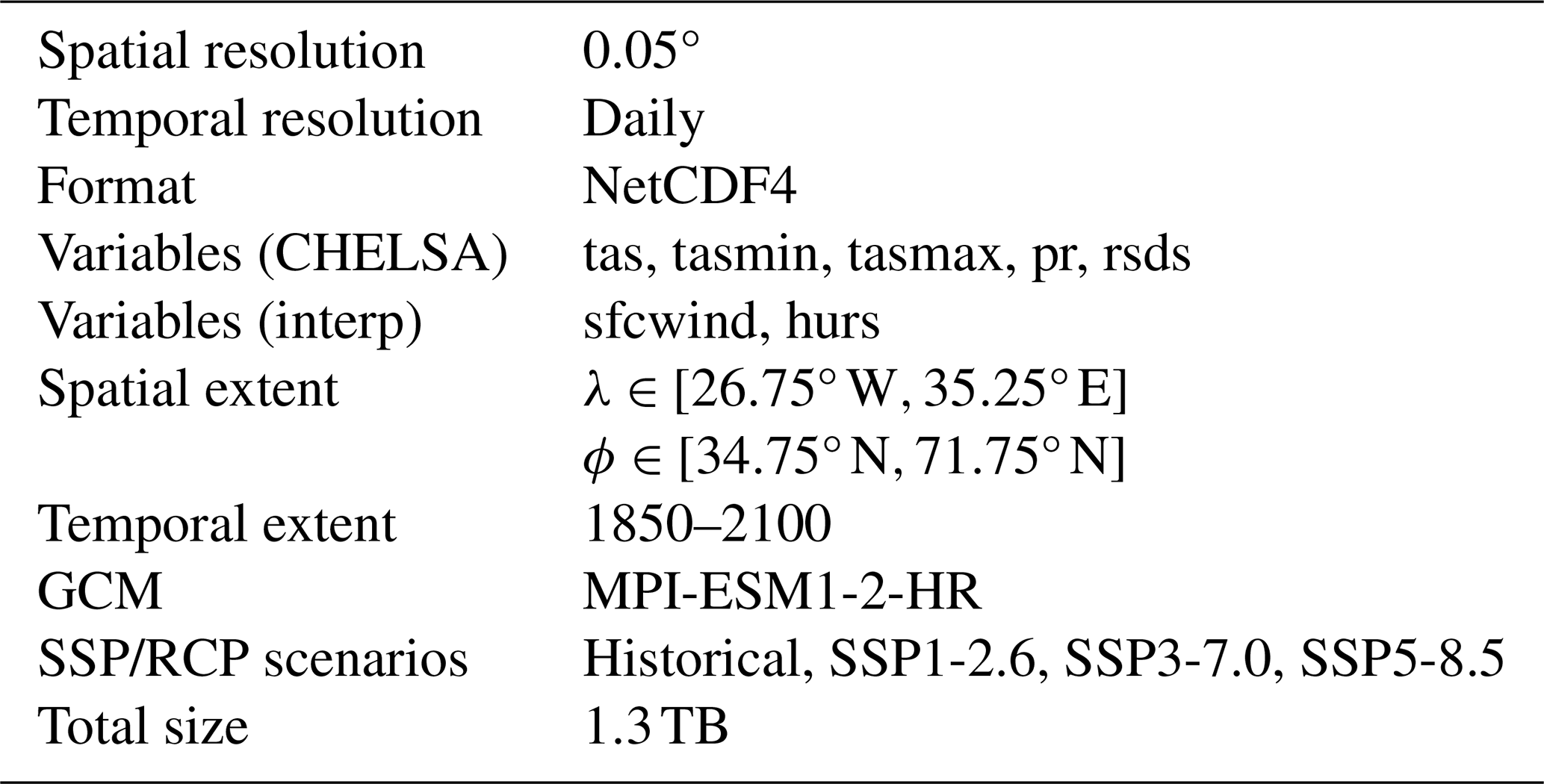
The CHELSA algorithm was used to downscale ISIMIP3b mean, maximum and minimum daily temperatures, precipitation rate, and downwelling solar radiation in the domain defined by $\mathit{\lambda }\in [\mathrm{26.75}\mathit{°}\mathrm{W},\mathrm{35.25}\mathit{°}\mathrm{E}]$; $\mathit{\varphi }\in [\mathrm{34.75}\mathit{°}\mathrm{N},\mathrm{71.75}\mathit{°}\mathrm{N}]$, where λ and ϕ are geographical longitude and latitude, respectively. This domain encompasses the continental European Union plus Norway, Iceland, Switzerland, the United Kingdom, the non-EU Balkan states, Moldova, Belarus, and parts of Ukraine, Russia, Morocco, Algeria, and Tunisia. CHELSA generates one TIFF file per day for each of the input variables at an output resolution of 0.0083(3)° (approximately 1 km near the Equator). LPJ-GUESS simulations covering the target domain at this resolution are computationally impractical. We thus first upscaled the files to 0.05° by taking the mean of every 6×6 block of adjacent 0.0083(3)° × 0.0083(3)° gridcells. This upscaled version was stored in NetCDF format. Gaps produced by missing days in CHELSA's output (∼0.34 % in the historical period, and fewer than 0.14 % in the scenarios) were filled with previous day values. The daily NetCDF files were stacked along the time dimension, and we added CF-compliant metadata (Hassell et al., 2017). LPJ-GUESS simulates the whole target period in one gridcell before proceeding to the next location. To optimize data retrieval by the model code, the stacked NetCDF files were rechunked along the time dimension. This operation rearranges the internal structure of the file in a way that greatly enhances performance when reading the full time series at a single spatial location. The resulting files underwent quality control, which included checking that there were no missing days, ensuring that all values were non-negative, and manually assessing that annual mean values were reasonable. In addition to the variables downscaled with CHELSA, we remapped ISIMIP3b near-surface wind speed and air relative humidity data to high resolution by applying bilinear interpolation to the original files. These variables are required when running LPJ-GUESS with the SIMFIRE/BLAZE fire model (Knorr et al., 2014, 2016; Rabin et al., 2017) (see Sect. 5). The CHELSA original algorithm depends on a B-spline interpolation for wind, while we adopt here bilinear interpolation. Both techniques derive from the same class-polynomial interpolation, and bi-linear interpolation is expected to capture terrain heterogeneity better. Relative humidity is not included in the original CHELSA approach. The pipeline scripts were implemented in Bash Script and Python, and use the NetCDF Operators (Zender, 2008) and the Climate Data Operators (Schulzweida, 2023).

Table 1 summarizes the properties of the dataset. The data is freely accessible through KIT/IMK-IFU's thredds storage server Otryakhin and Belda (2024), and is made available under the CC BY-SA 4.0 license.

Table 1 Characteristics of the final downscaled dataset. Variable names follow the ISIMIP3b nomenclature: daily average temperature, minimum, and maximum (“tas”, “tasmin”, “tasmax”), precipitation (“prec”), downwelling shortwave radiation (“rsds”), wind speed (“sfcwind”), and relative humidity (“hurs”).

4 Ensemble experiment

4.1 Setup

This experiment aims to find systematic differences in regional predictions between low- and high-resolution LPJ-GUESS simulations, arising from underrepresentation of orography-induced climate variability in the low-resolution forcings. To this end, we ran two sets of ensembles of LPJ-GUESS simulations (high- and low-resolution) in selected study and control regions. The simulations spanned the historical period 1850–2014. The low-resolution simulations were forced with ISIMIP3b climate, while the high-resolution simulations were forced with the downscaled dataset. Both simulations use the same soil properties dataset, derived from the Digitized Soil Map of the World (Zobler, 1986), as in Sitch et al. (2003). In order to prevent introducing possible confounding factors, the soil information was not downscaled, and we kept nitrogen deposition at a constant pre-industrial rate of 2 kgN ha⁻¹ yr⁻¹. We chose the Alps as our study region for its high variability in surface elevation. The control region, located between the Dinaric Alps and the Carpathian Mountains, was chosen to contain comparatively little mountainous terrain (Table 2), while being in close proximity to the Alpine region and of approximately the same size. The climate between the Pannonian basin and the European alps naturally differs but is still influenced by similar, large-scale circulation patterns that affect the European continent and the choice of the control region intended to prevent significant global differences. Figure 1 shows the study and control regions overlayed on an elevation map. The gridcell centers were chosen such that any low-resolution gridcell contains a block of 10×10 high-resolution gridcells, with no high-resolution gridcells outside these blocks (i.e., a perfect overlap of the high- and low-resolution grids). Prominent water bodies were avoided.

Table 2 Characteristics of elevations in the study and the control regions computed using values from GMTED2010 (Danielson and Gesch, 2011). All values are in meters.

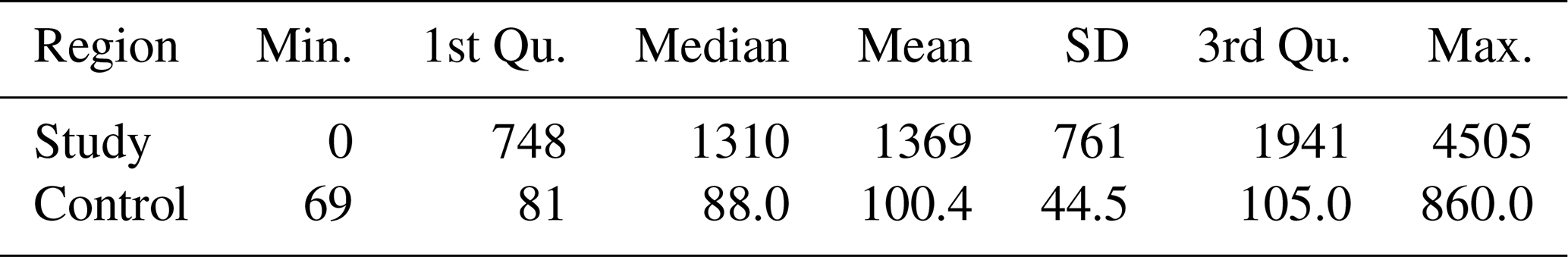
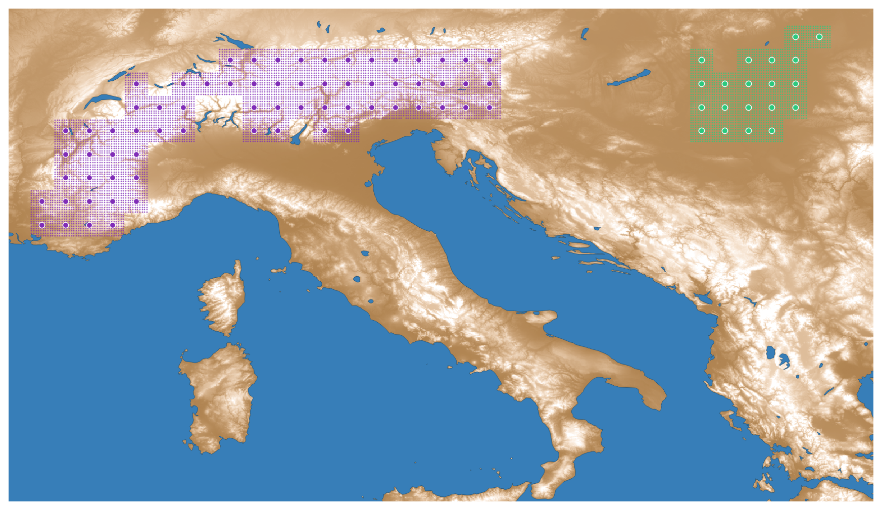
Figure 1 Study (violet) and control (green) regions for the ensemble experiment, overlaid on an elevation map based on values of GMTED2010 (Danielson and Gesch, 2011). The centers of low-resolution gridcells are indicated by solid circles. The smaller dots mark the location of the high-resolution gridcells. Elevation is encoded as a color gradient ranging from dark brown (low elevation) to white (high elevation).

The experimental design is outlined in Fig. 2. We considered the regional averages of each modeled variable (Table 3), evaluated in the last year of the simulation (2014), as random variables. We run 50 simulations per region and resolution, giving rise to 44 ensembles of random variables (11 modeled variables/simulation × 2 resolutions × 2 regions), each containing 50 observations of its random variable. For a given region and resolution, the simulations were identically set up, but used a different seed for the random number generator (see Sect. 2.3.2). Model runs were assumed to be independent and identically distributed. We note that such an assumption is not imposed on pairs of ecosystem variables within the same model run. The patch number was set to 20 in all simulations.

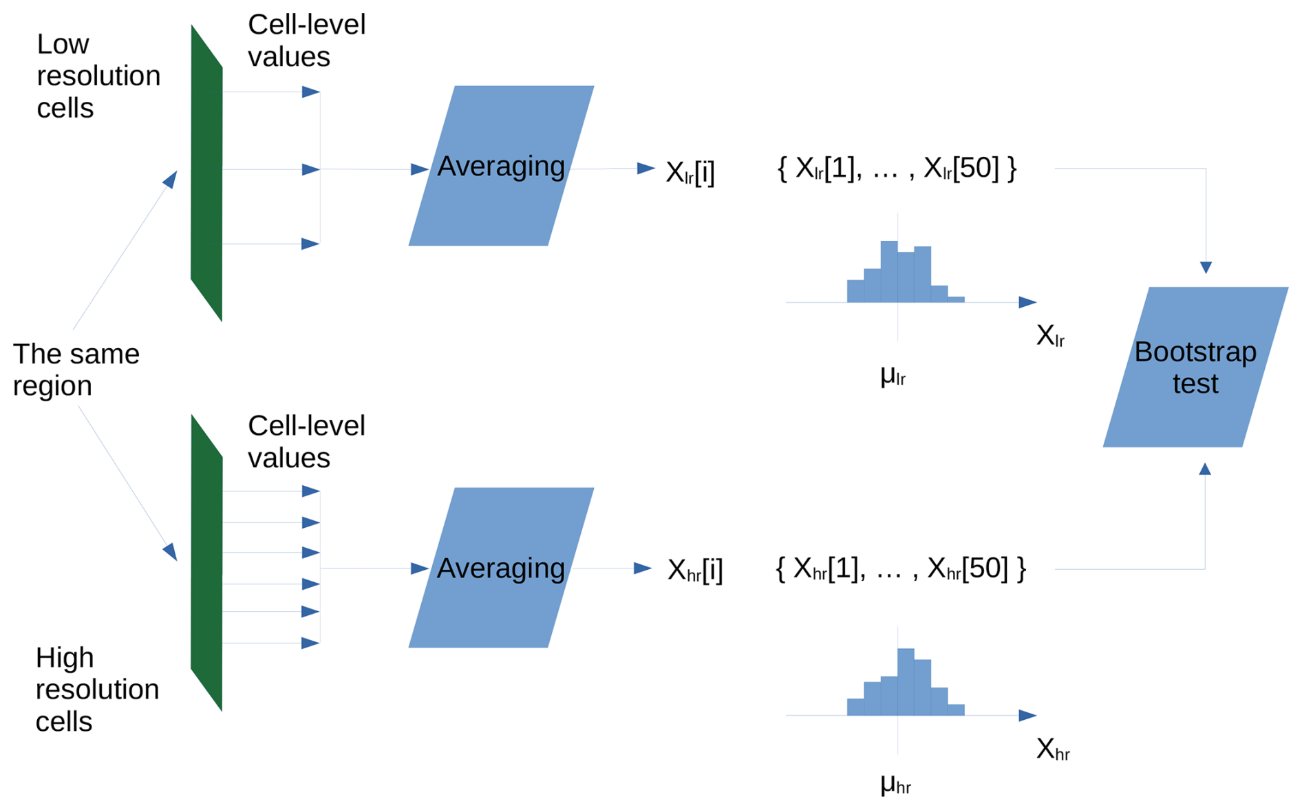
Figure 2 Scheme of computations in the ensemble experiment. Here, X is the average of values at the end of the computation period 1850–2014 in the region, lr and hr are the indicators of the low and high resolution correspondingly, $i=\mathit{\{}\mathrm{1},\mathrm{\dots },\mathrm{50}\mathit{\}}$ is the experiment id, μ's are the sample mean estimates.

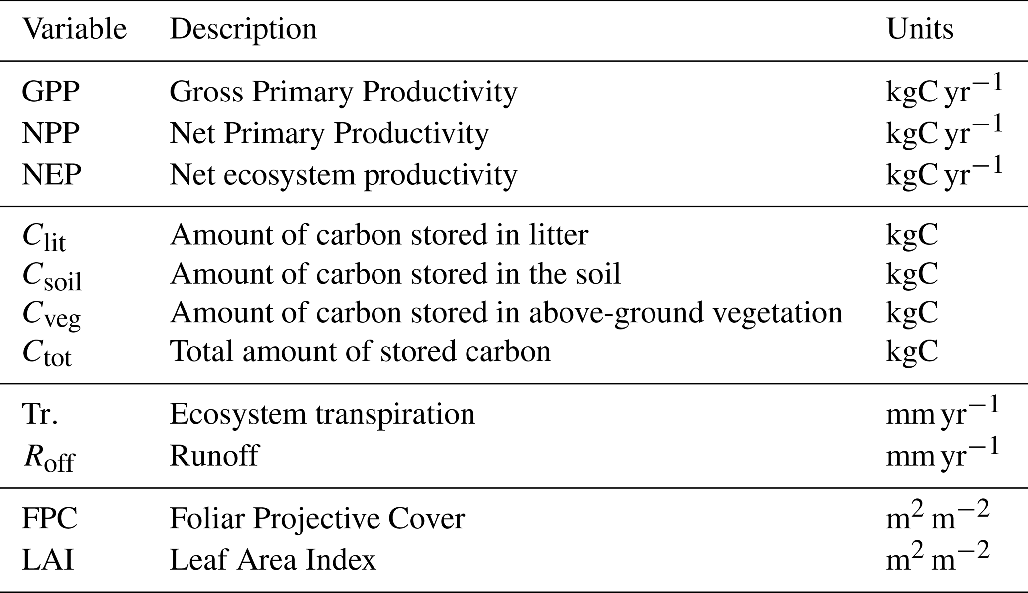
Table 3 List of ecosystem variables modeled by LPJ-GUESS that were included in the experiment. These include carbon fluxes (GPP, NPP, and NEP), carbon pools (C_lit, C_soil, C_veg, and C_tot), water cycle variables (Tr. and R_off), and vegetation structural variables (FPC and LAI). The units refer to regional aggregates (for all variables except FPC and LAI) and regional averages (for FPC and LAI) of the selected variables.

Let ${\mathit{\mu }}_{\mathrm{hr}}^{\mathrm{S}}$, ${\mathit{\mu }}_{\mathrm{lr}}^{\mathrm{S}}$, ${\mathit{\mu }}_{\mathrm{hr}}^{\mathrm{C}}$, and ${\mathit{\mu }}_{\mathrm{lr}}^{\mathrm{C}}$ denote the ensemble means of any of the modeled variables, with superscripts “S” and “C” identifying the study and control regions, and subscripts “hr” and “lr” denoting high- and low- resolution. The question of whether there are systematic differences between low- and high-resolution regional predictions in areas with high orographical variability can be cast in terms of two formal hypothesis tests:

$$\begin{array}{}\text{(18)}& \begin{array}{rl}& H_{\mathrm{o}}^{\mathrm{S}}:{\mathit{\mu }}_{\mathrm{hr}}^{\mathrm{S}}={\mathit{\mu }}_{\mathrm{lr}}^{\mathrm{S}}\text{(There are no differences in the study region)}\\ & \text{vs.}\\ & H_{\mathrm{a}}^{\mathrm{S}}:{\mathit{\mu }}_{\mathrm{hr}}^{\mathrm{S}}\ne {\mathit{\mu }}_{\mathrm{lr}}^{\mathrm{S}},\text{(There are differences in the study region)},\end{array}\end{array}$$

and

$$\begin{array}{}\text{(19)}& \begin{array}{rl}& H_{\mathrm{o}}^{\mathrm{C}}:{\mathit{\mu }}_{\mathrm{hr}}^{\mathrm{C}}={\mathit{\mu }}_{\mathrm{lr}}^{\mathrm{C}}\text{(There are no differences in the control region)}\\ & \text{vs.}\\ & H_{\mathrm{a}}^{\mathrm{C}}:{\mathit{\mu }}_{\mathrm{hr}}^{\mathrm{C}}\ne {\mathit{\mu }}_{\mathrm{lr}}^{\mathrm{C}},\text{(There are differences in the control region)}.\end{array}\end{array}$$

where the subscript “o” denotes the null hypotheses and “a” identifies the alternatives. We tested these hypotheses for every variable by applying the bootstrap test method described in Sect. 2.2.

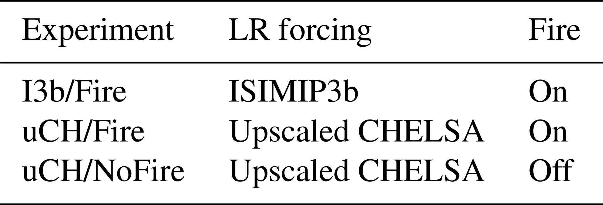
CHELSA conserves the amount of precipitation in the upscaled output by construction (Sect. 2.1.2), but does not impose such constraint on mean temperature and radiation. In order to investigate the possible biases associated with this non-conservative downscaling we repeated the above experiment, this time forcing the low-resolution simulations with CHELSA climate, upscaled back to 0.5° by spatially averaging the high-resolution data. This ensures that mean temperature, radiation and precipitation are the same on both resolutions. In addition, we wished to investigate the impact of fire disturbance on the results of the above experiments. This was motivated by the fact that, in LPJ-GUESS, fire disturbance depends on the climate forcings through the fire model (Rabin et al., 2017). To explore this effect we rerun the last experiment with fire switched off. The characteristics of the three ensemble experiments are summarized in Table 4.

Table 4 Ensemble experiments carried out in Sect. 4. The experiments differ in the climate data used to force the low-resolution simulations and on whether wildfires are allowed.

4.2 Results and analysis

The results of the first experiment (I3b/Fire) are shown in Table 5. We found statistically significant differences between the means of the high- and low-resolution samples (${\mathit{\delta }}^{\mathrm{S}}:={\mathit{\mu }}_{\mathrm{lr}}^{\mathrm{S}}-{\mathit{\mu }}_{\mathrm{hr}}^{\mathrm{S}}$) over the study region. The bootstrap test returned a p-value of 0 for all the variables, leading us to reject $H_{\mathrm{o}}^{\mathrm{S}}$ in favor of the alternative $H_{\mathrm{a}}^{\mathrm{S}}$.

Table 5 Results of the I3b/Fire experiment. The ensemble means and standard deviations are denoted μ and σ, respectively. The superscripts S and C identify the study and the control regions, respectively. The subscripts hr and lr denote high- and low-resolution. The δ is used for the difference between the low- and high-resolution ensemble means for the given region. The p^S and p^C denote the p-values for the statistical tests defined by Eqs. (18) and (19). The p^X are the p-values for the test defined in Sect. 4.2. A bold font face is used to identify tests with a p-value below the significance threshold. The ratios ${\mathit{\delta }}^{\mathrm{S}}/{\mathit{\mu }}_{\mathrm{hr}}^{\mathrm{S}}$, ${\mathit{\delta }}^{\mathrm{C}}/{\mathit{\mu }}_{\mathrm{hr}}^{\mathrm{C}}$, and ${\mathit{\delta }}^{\mathrm{S}}/{\mathit{\delta }}^{\mathrm{C}}$ are expressed as percentages.

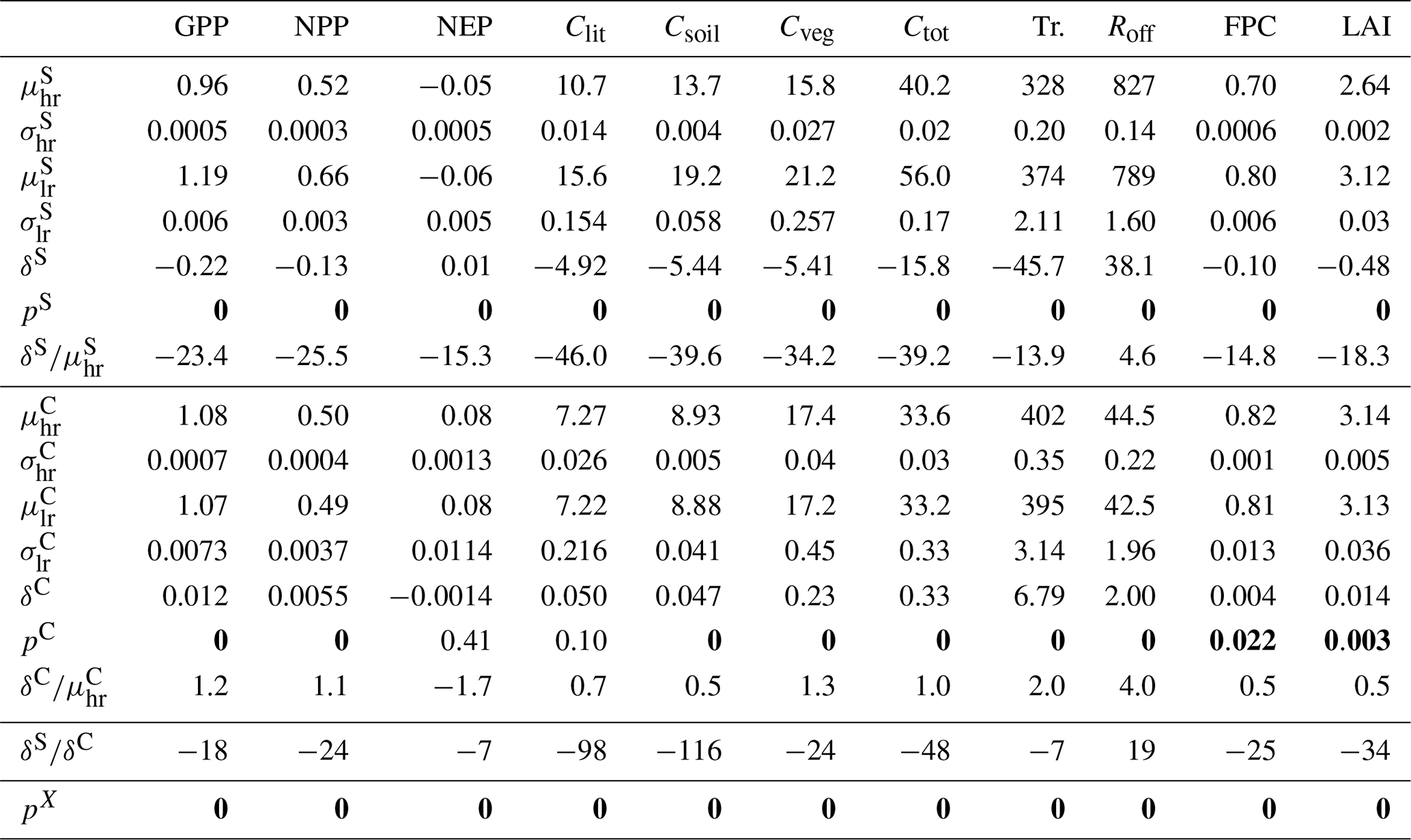
In the control region all differences between ensemble means, ${\mathit{\delta }}^{\mathrm{C}}:={\mathit{\mu }}_{\mathrm{lr}}^{\mathrm{C}}-{\mathit{\mu }}_{\mathrm{hr}}^{\mathrm{C}}$, are substantially smaller than their study region counterparts, ranging from $|{\mathit{\delta }}^{\mathrm{S}}/{\mathit{\delta }}^{\mathrm{C}}|\sim \mathrm{7}$ in the case of NEP and Transpiration to ∼116 in the case of C_soil. For the majority of the variables, the p-values indicate a statistically significant difference between ensemble means δ^C. For NEP and C_lit, however, we found no evidence in the data to reject the null hypothesis $H_{\mathrm{o}}^{\mathrm{C}}$. This indicates that, for these two variables, either there are no significant differences between ${\mathit{\mu }}_{\mathrm{lr}}^{\mathrm{C}}$ and ${\mathit{\mu }}_{\mathrm{hr}}^{\mathrm{C}}$, or the ensemble size is too small to detect them with a sufficient confidence level. Figure 3 shows δ^S and δ^C, as a fraction of μ_hr, for all variables. These values in the study region have the opposite sign to those in the control region, with the exception of NEP and R_off.

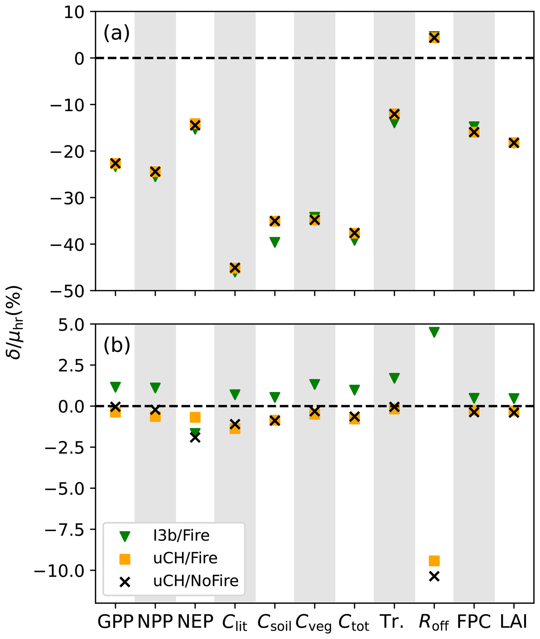
Figure 3 Mean difference between high- and low- resolution ensemble means, as a percentage of the high-resolution ensemble mean, over the study region (a) and the control region (b). The different symbols represent the three experiments; I3b/Fire: low-resolution simulations are forced with ISIMIP3b climate; uCH/Fire: low-resolution simulations are forced with upscaled CHELSA climate; uCH/NoFire: low-resolution simulations are forced with upscaled CHELSA climate and fire is switched off.

An additional bootstrap test was run to check whether random variability in the control region could give rise to differences between ensemble means as large as those seen in the study region. With low- and high-resolution values in place of X_i and Y_i, we generated the distribution of T^* from the left side of Eq. (16), and found the two-sided p-values using $-\left|{\mathit{\delta }}^{\mathrm{S}}\right|$ and $+\left|{\mathit{\delta }}^{\mathrm{S}}\right|$. These tests returned a p-value p^X=0 for all variables, which strongly suggests that control-region differences as large as those found in the study region could not be explained by mere random variability of the ensemble means.

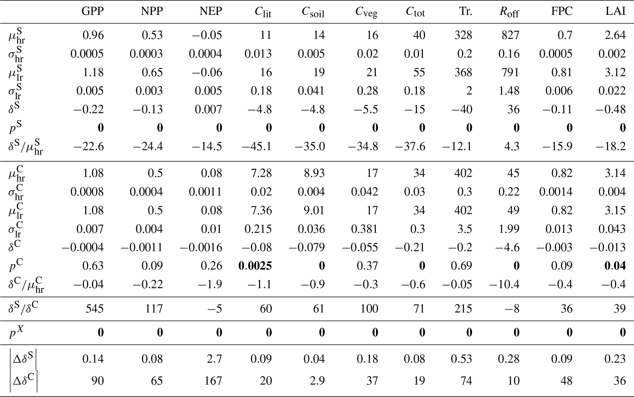
Table 6 Results of the uCH/Fire experiment. Repeated symbols are as in Table 5. |Δδ^S| and |Δδ^C| are the changes in magnitude of δ^S and δ^C with respect to I3b/Fire, expressed as a percentage.

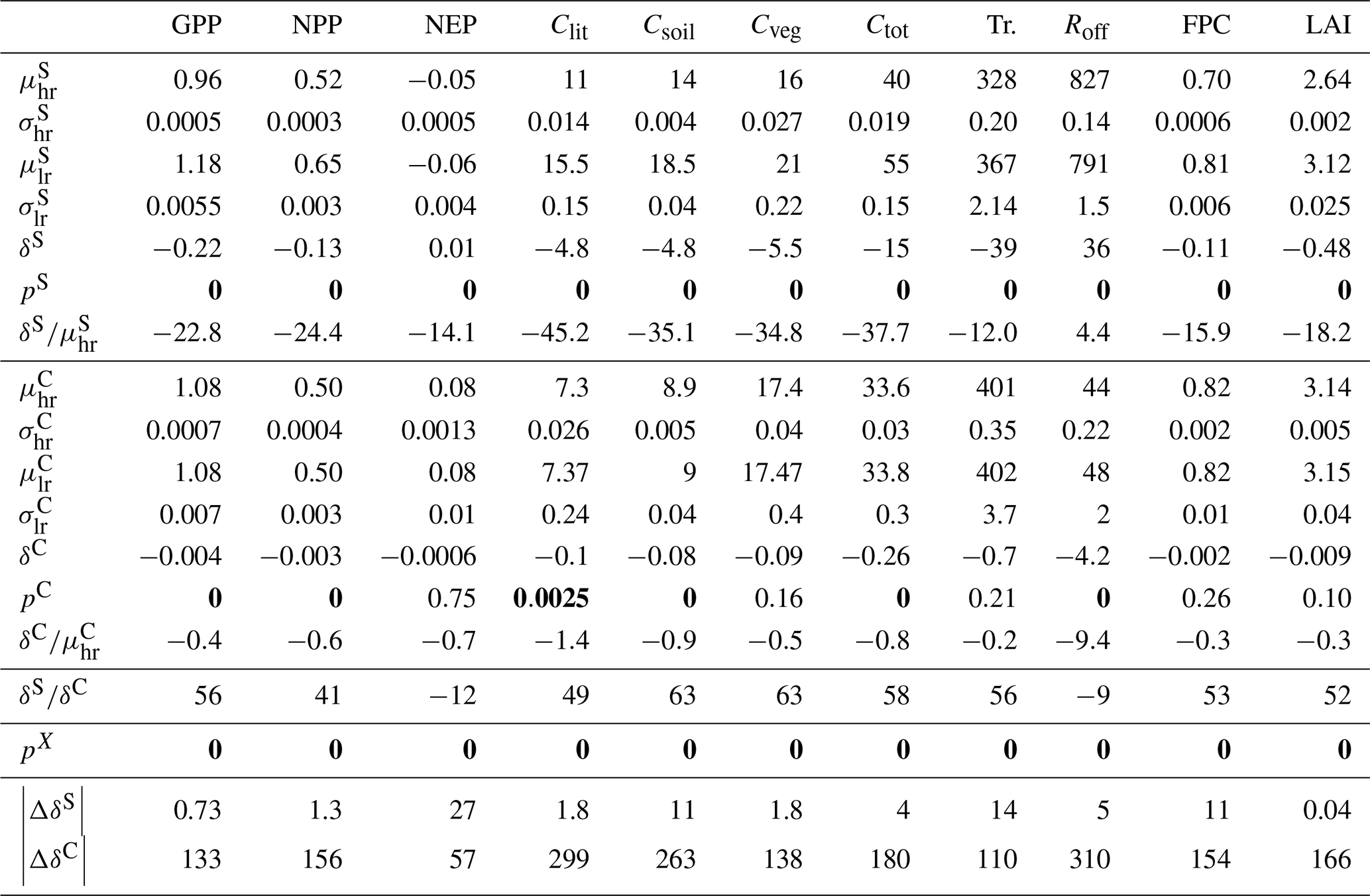
Table 6 shows the results of the second experiment (uCH/Fire). All bootstrap tests returned a p-value of 0 in the study region, again indicating very strong evidence of a mean difference between high- and low-resolution outputs. In the control region, 5 of 11 tests failed to reject the null hypothesis: NEP, C_veg, Tr., FPC, and LAI. Interestingly, the C_lit test switched to returning a significant p-value. The relative differences between ensemble means in the study and control regions, ${\mathit{\delta }}^{\mathrm{S}}/{\mathit{\mu }}_{\mathrm{hr}}^{\mathrm{S}}$ and ${\mathit{\delta }}^{\mathrm{C}}/{\mathit{\mu }}_{\mathrm{hr}}^{\mathrm{C}}$, are now both negative (Fig. 3) except for the high-resolution R_off. Runoff shows the largest relative discrepancy with respect to the previous experiment, but the difference in absolute terms is very small. This sign switch of δ^C with respect to I3b/Fire suggests that CHELSA's non-conservative properties introduce a bias of sign opposite to the response of the model to the altitude-driven climate differences. The relative importance of this effect is much larger over the control region, where it determines the sign of the overall difference δ^C. The change in magnitude of δ^C with respect to I3b/Fire, |Δδ^C|, was between ∼110 % and ∼310 %, except for NEP (∼57 %). By contrast, |Δδ^S| is much smaller, ranging between ∼0.04 % and ∼14 %. This may explain the significance switch in the C_lit test over the control region; the non-conservative bias present in the I3b/Fire experiment nearly compensates the altitude-induced differences for this variable. This brings the high- and low-resolution means closer together, which makes it more difficult to discern them. When this bias is removed in uCH/Fire, the difference between ensemble means increases, and the bootstrap test is able to detect it.

The outcome of the uCH/NoFire experiment is shown in Table 7. Like before, the impact on the control region is comparatively larger than in the study region, as shown by the values of |Δδ^S| and |Δδ^C|, and by the fact that some of the tests in the control region returned switched p-values again.

Table 7 Results of the uCH/NoFire experiment. Repeated symbols are as in Table 5. |Δδ^S| and |Δδ^C| are the changes in magnitude of δ^S and δ^C with respect to uCH/Fire, expressed as a percentage.

We summarize the analysis described in this section as follows. It was demonstrated that high- and low-resolution simulations produce significantly different average predictions over a study region with high elevation variability. Differences in the control region were also detected, but they are much smaller than in the study region. Climate data downscaled with CHELSA introduces a bias related to its non-conservative treatment of temperature and radiation. This bias is comparable in magnitude to the altitude-related differences in the control region, but small in relation to the magnitude of the variables, and largely inconsequential in the study region. When this bias was removed, average NEP, C_veg, Tr., and FPC were indistinguishable in the high- and low-resolution simulations. Fire was found to be a significant contributor to the ensemble mean differences in the control region.

CHELSA-downscaled climate data is closer to observations than the original, coarse resolution data (Karger et al., 2021, 2023). This motivates us to consider the difference between high- and low-resolution simulations as a systematic bias incurred when running LPJ-GUESS at low resolution, arising from the underrepresentation of orographical climate variability.

5 Comparison of Europe-wide simulations

5.1 Setup

In order to assess the impact of systematic biases in low-resolution LPJ-GUESS outputs on a European-regional level, we ran two simulations, at high and low resolutions, in the European domain from Sect. 3 (Table 1). The input to the model is as in the ensemble experiment, except now we use historical ISIMIP nitrogen deposition data (Tian et al., 2018). Both simulations were fed with the original 0.5° × 0.5° data. To capture coastline features and inland water bodies as accurately as possible for each resolution, we drop the restriction of one-to-one correspondence between blocks of 10×10 high-resolution gridcells and the low-resolution ones (see Sect. 4.1). The number of patches was set to 100 for both runs, and wildfires were enabled.

5.2 Analysis and results

Forcing LPJ-GUESS with low-resolution climate data introduces a bias in average predictions, related to the underrepresentation of climate spatial variability (Sect. 4). Figure 4 shows this climate-response bias for GPP, averaged over the 2010–2014 period. Similar maps for the rest of the variables can be found in the Supplement (Sect. S1: Supplement to Comparison of Europe-wide simulations). The most prominent discrepancies concentrate over highly mountainous regions, such as the Alps, the Spanish mountains and the Scandinavian Mountains. Large differences are also seen in Iceland, where the rapidly changing elevation leads to high spatial variability above and below the low-resolution predictions.

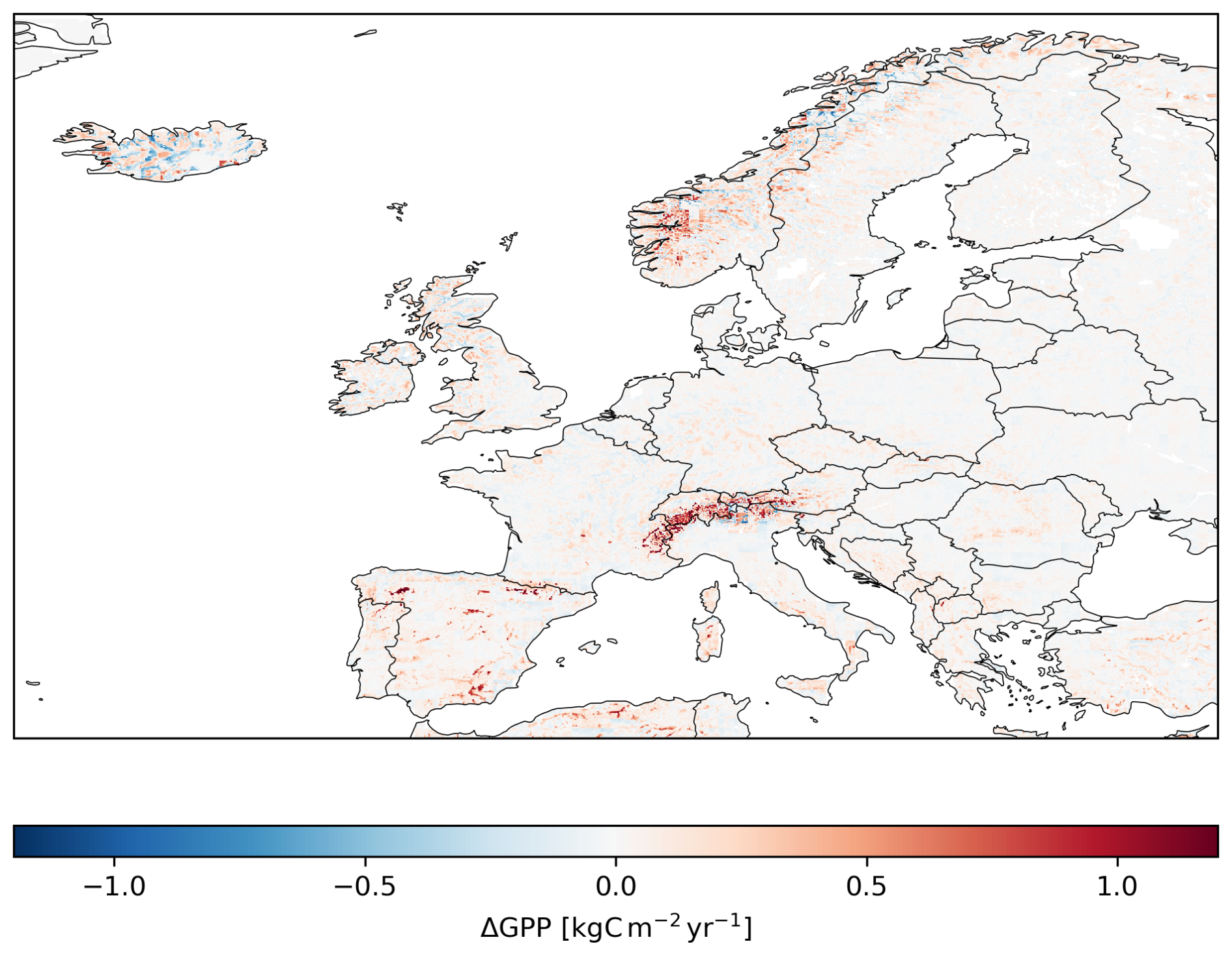
Figure 4 Climate-response bias in low-resolution modeled GPP, calculated as the difference between the low- and high-resolution predictions, averaged over the period 2010–2014. The value from every high-resolution gridcell was subtracted from the value in the corresponding 10×10 low-resolution block. Only fully overlapping low- and high- resolution gridcells are represented. Red indicates a higher GPP value in the low-resolution run than in the high-resolution run.

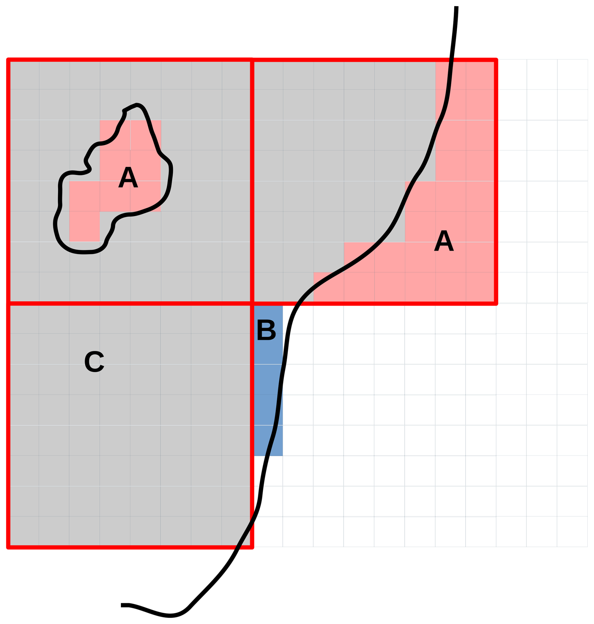
Figure 5 Three low-resolution gridcells (outlined in red) projected onto a high-resolution grid. A small lake and the coastline are represented with black, thick lines. The sea is to the right of the coastline. Red-shaded regions (marked A) indicate areas that are considered land in low-resolution simulations and water in high-resolution simulations. The blue-shaded area (marked B) is accounted for in a high-resolution run, but not in a low-resolution run. Gray areas (marked C) are represented in both high- and low-resolution simulations. White areas are considered water points in both simulations.

Additional bias results from the limitations of the low-resolution grid in representing areas around coastlines and inland water bodies (Fig. 5). In a low resolution simulation, some gridcells protrude outside the coastline, thus covering some sea-surface area (marked A), which is simulated as land. Similarly, the low-resolution grid cannot resolve small lakes, which adds to the overestimation of land-surface area. By contrast, some land-surface areas close to the seashore (marked B) are correctly accounted for in high-resolution simulations, but cannot be captured in low-resolution. In the European domain under consideration, these two counteracting effects amount to a ∼3.5 % increase in simulated surface area in the low resolution runs. This leads to a shoreline-representation bias in regional estimates.

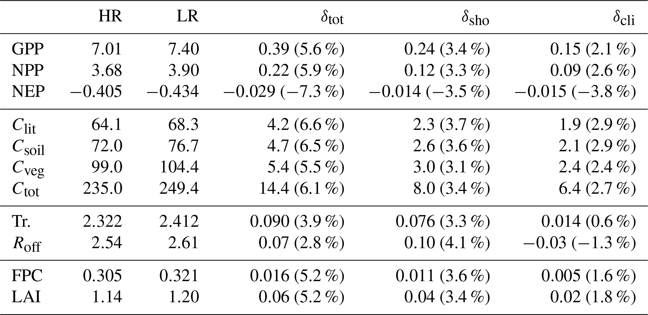
Aggregating GPP across the domain yields an average of 7.01 PgC yr⁻¹ over the period 2010–2014 for the high-resolution simulation, and 7.40 PgC yr⁻¹ for the low-resolution simulation (a 5.6 % increase). The climate-response and shoreline-representation contributions to this increase are δ_cli=2.1 % and δ_sho=3.4 %, respectively. Table 8 shows aggregate high- and low-resolution values for the rest of the selected variables. In this region, the shoreline-representation bias is larger in magnitude than the climate-response bias for all variables. The largest relative discrepancy is seen in C_lit; a 6.6 % increase respect to the high-resolution value, with contributions δ_cli=2.9 % and δ_sho=3.7 % (the bias in NEP is even larger, but NEP is a very small quantity resulting from the difference of two large quantities (GPP and ecosystem respiration), and hence very sensitive to small variations in either of those terms. In the case of aggregate runoff, the shoreline-representation bias (δ_sho=4.1 %) and the climate-response bias (${\mathit{\delta }}_{\mathrm{cli}}=-\mathrm{1.3}$ %) act in opposite directions, adding up to a net total of δ_tot=2.8 %. The calculation of the climate-response and shoreline-representation contributions to the total bias is detailed in Appendix A.

Table 8 Comparison of domain-wide aggregates of selected ecosystem variables for the high- and low- resolution European simulations (HR and LR, respectively). δ_tot is the total bias, δ_sho is the shoreline-representation bias, and δ_cli is the bias arising from the difference in climate forcings. Percentages are calculated with respect to the high-resolution values.

6 Discussion

Earlier work by Müller and Lucht (2007) showed little impact on model results when running the LPJ DGVM between 10° and 0.5°, at 0.5° intervals, suggesting that a resolution of 0.5° is still too coarse to account for relevant effects of spatial heterogeneity. Our study suggests that the impacts of resolution on the modeled output, linked to the influence of orography on the input climate, become noticeable at higher resolutions. The relative importance of these effects strongly depends on the focus region. Europe-wide simulations show an impact of resolution on aggregated ecosystem pools and fluxes of ∼3 %, likely smaller than the uncertainty derived from the spread in climate forcings by different GCMs (see, e.g., Schaphoff et al., 2006; Morales et al., 2007; Schurgers et al., 2018). By contrast, these differences increase up to ∼46 % in an Alpine region. Additional bias may result from poor representation of shorelines and small inland water bodies, but this effect could be mitigated by scaling the model output by the land-cover fraction in the affected gridcells. In areas of low variability in surface elevation, the difference between LPJ-GUESS outputs at different resolutions is much smaller and may be safely ignored in calculations involving regional averages of ecosystem variables. For this type of studies, one could optimize the resource requirements of the simulations by using a coarser resolution in areas with low elevation variability.

The high-resolution simulations were performed on a grid that captures coastlines and water bodies more precisely, and are driven by climate that is generally closer to the observed regional climate (see validation sections in Karger et al., 2021, 2023). This motivates us to interpret these differences as systematic biases incurred when running LPJ-GUESS on a coarse grid. We defer evaluating the simulation results against observational data to future studies. However, we note here that if the model output on low resolution was closer to observations, that would suggest that the model needs recalibration or revision.

Since geographical features and climate effects are not related to intrinsic properties of LPJ-GUESS, we infer that predictions by other DGVMs are likely to be affected in a similar manner. We note, however, that gridcells in LPJ-GUESS are independent of each other (there is no lateral information flow) and completely unaware of gridcell size. By contrast, other models may include processes, such as lateral matter transport, which are sensitive to the coarseness of the grid. This introduces an additional dependence of the output on resolution, on top of the effects discussed in this study.

One possible mechanism underpinning the difference in modeled GPP between high- and low-resolution simulations in areas with high elevation variability is the non-linear relationship between the mean gridcell temperature and the duration of the growing season, which is dynamically calculated by LPJ-GUESS. The linear relationship between temperature and elevation (Eqs. 1 and 2) implies that air temperatures in higher parts of resolved mountainous areas are lower than the average value in the corresponding low-resolution gridcell (Fig. 6), causing a shorter growing season. The lower parts will, in turn, experience a longer growing season. The shorter growing season in high areas leads to reduced productivity and vegetation cover. Because of the non-linear response of the model to climate forcings, this is not fully compensated by the additional productivity in the lower, warmer parts. A similar argument can be made for the photosynthetic rate, which is temperature-dependent.

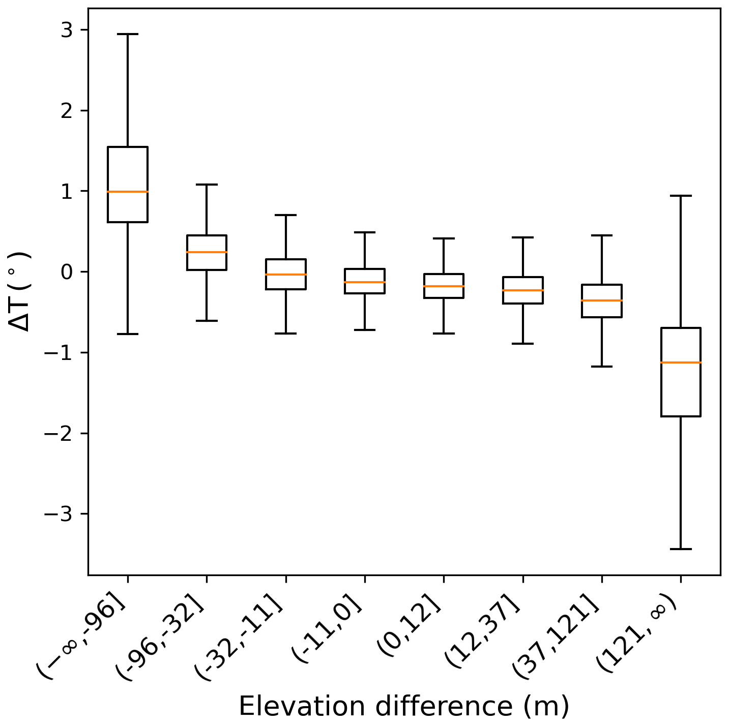
Figure 6 Distribution of the difference in mean air temperature between the downscaled and the original datasets. Positive values indicate a temperature increase after downscaling. The data was binned in octiles of elevation difference, calculated with respect to the average elevation of the low-resolution gridcell that contains the data point. The x-axis labels indicate limits of the bins. Water points are excluded. The distributions were derived from temperature averages over the 2011–2014 period.

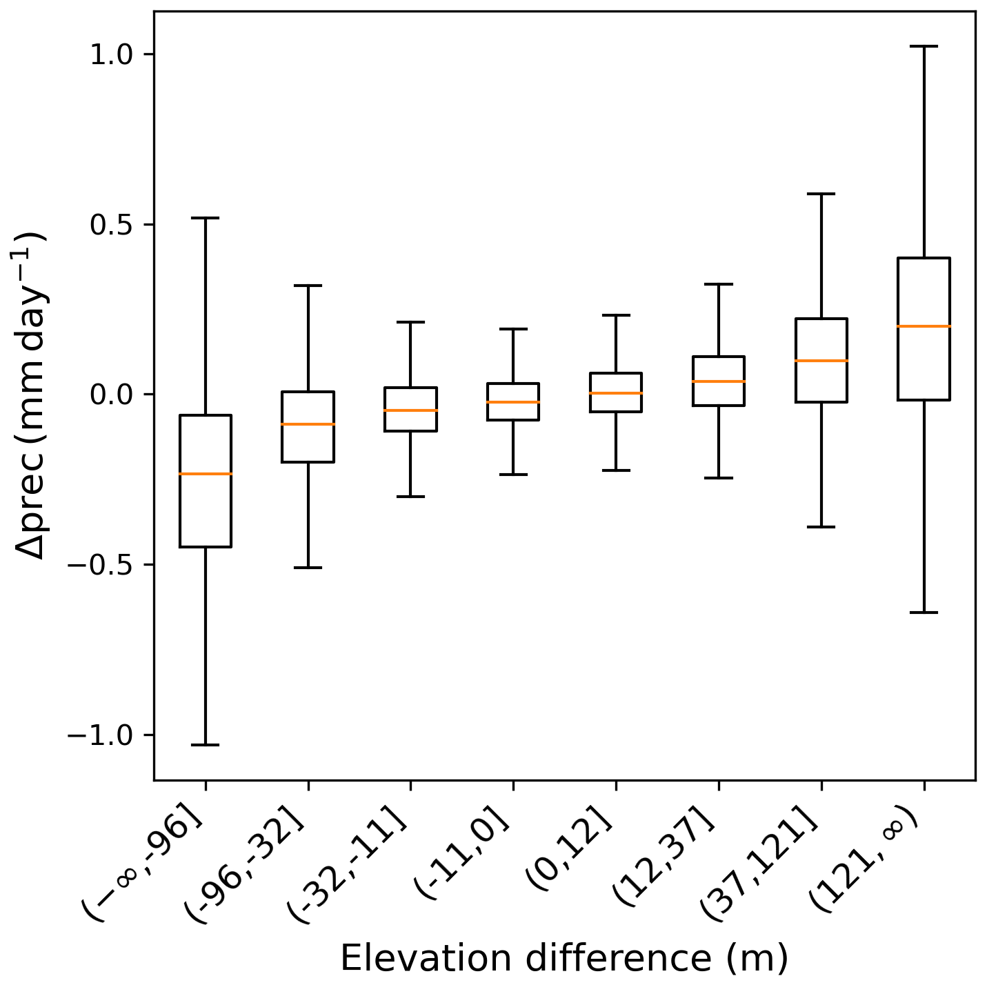
On the other hand, rainfall redistribution in the high-resolution grid may provide a counteracting effect. CHELSA tends to concentrate the total amount of rainfall towards high-elevation areas to account for the influence of orography on precipitation (Fig. 7), which may reduce water availability for plant growth in the lower areas.

Figure 7 As in Fig. 6, but for average precipitation.

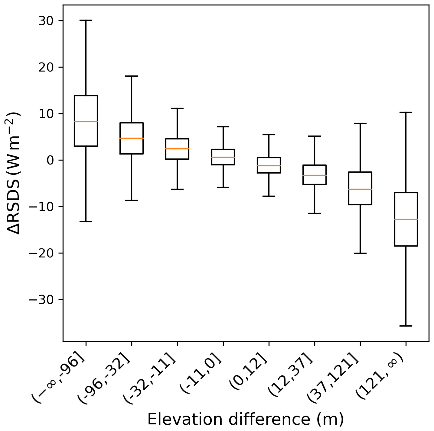
The radiation downscaling algorithm is more involved, and includes the effects of orographical features as well as those of the position of the Sun (Sect. 2.1.3). Nonetheless, there is a clear pattern in Fig. 8 showing that higher parts of mountains receive less solar radiation per square meter than the corresponding low-resolution value, while the lower parts – more. This suggests that the increased cloud cover resulting from orographic precipitation leads to a decrease in average radiation in areas of higher elevation difference. This effect contributes to the reduction of vegetation in places with high elevations.

Figure 8 As in Fig. 6, but for average RSDS.

Another counteracting factor is the excess land simulated in a grid too coarse to resolve small inland water bodies. The interplay between these factors will depend on the specific region being simulated, which emphasizes the complexity of the model's response to orographical and climate drivers.

There are many other modeled processes that respond non-linearly to climate forcings. Leaf-level photosynthesis shows a saturating (as opposed to linear) response to absorbed photosynthetically-active radiation when not limited by RuBisCo production (see Haxeltine and Prentice, 1996, for a discussion of the scaling of leaf-level photosynthesis to canopy-level productivity). Soil water transport follows a power law of available water content, which in turn depends on the amount of rainfall (see Gerten et al., 2004). The amount of radiation reaching the forest floor, which determines potential establishment of new saplings, obeys an exponential law that depends on the forest canopy's LAI (Monsi and Saeki, 1953, 2005). The decay rate of C in the different soil carbon pools is a non-linear function of soil temperature (driven by air temperature in the model) and soil water content (which depends non-linearly on precipitation rate, as mentioned above; see description of the carbon cycle submodel in Smith et al., 2014).

The effect of fire on simulation results was found to be somewhat important, but not as strong as those of non-conservative properties of CHELSA and differences in climate due to orography. The effect includes 2 parts. First, since ignition is stochastic, the presence of the fire module may be able to increase the variation of the simulation results. Comparison of the standard deviations in Tables 6 and 7 shows that this effect does not play a significant role. Second, fire is a rare but destructive event which introduces changes in the potential vegetation structure. This could be one of the reasons why we see more variables with statistically indistinguishable ${\mathit{\mu }}_{\mathrm{hr}}^{\mathrm{C}}$ and ${\mathit{\mu }}_{\mathrm{lr}}^{\mathrm{C}}$ in the uCH/NoFire experiment than in the uCH/Fire one. In the study region on the high resolution, ignition is expected to occur more in valleys, which are warmer and drier than mountain tops, thus the effect of reduced vegetation in mountainous areas should be decreased in the uCH/NoFire experiment. However, in Fig. 3 we see that the influence of fire on vegetation in the study region is negligible compared to the influence of orography-induced climate difference.

Systematic biases in model outputs may arise as a consequence of differences in forcings other than resolution. For instance, high-resolution simulations might be sensitive to the algorithm used to downscale the forcings. In the context of climate change mitigation, correlations between different climate variables might influence relevant modeled variables (Zscheischler et al., 2019). To give an example of mechanisms responsible for these correlations, we notice that at points where light is obstructed, the temperature is lower than at neighboring points with no obstruction. Analogously, a spot with a significant amount of precipitation would be colder and darker than the same spot without precipitation. Such correlations are not built into univariate methods like CHELSA but can be captured by dynamical or multivariate downscaling methods. These methods are, however, generally more complex, and might require intensive use of computational resources. Therefore, it might be of interest to find systematic differences between simulations forced by the different methods. This could be done with the help of the methodology presented in Sects. 2.2 and 4. A similar setup could also be employed to investigate systematic differences originating from alternative model configurations. For example, one could assess whether the modeled impacts of two different forest managing strategies on regional carbon sinks are significantly different from each other.

7 Summary

In this paper we presented a high-resolution climate dataset for ecosystem modeling applications in Europe. We applied the CHELSA semi-mechanistic algorithm to scale four ISIMIP3b scenarios (historical, SSP1-2.6, SSP3-7.0, and SSP5-8.5) from an original resolution of 0.5° down to 0.05°. Further processing involved quality checks, rechunking to optimize time-series retrieval at a single location, and the addition of CF-compliant metadata. The new dataset is provided in NetCDF format (one file per variable), and is publicly accessible under a CC BY-SA 4.0 license.

We studied systematic differences between high-resolution LPJ-GUESS simulations, forced with the new dataset, and low-resolution simulations. We found that low-resolution simulations are systematically biased. Two main sources of bias were identified: (a) bias associated to the non-linear response of the model to orographical climate variability, and (b) bias associated to the poor representation of coastlines and inland water bodies on a coarse grid. While the latter may be mitigated by rescaling the output by the land cover fraction in the affected gridcells, reducing the climate-response bias requires a finer grid resolution. These sources of bias are independent of the downscaling algorithm, and apply to other DGVMs, insofar as their response to climate forcings is non-linear. Climate-response bias can be very large in mountainous areas; low-resolution simulations overestimated average predictions between ∼4 % and ∼45 % in an alpine region, as opposed to a mean bias of ∼1.4 % in a nearly-flat control region. Biases as large as in the alpine region were shown to be vanishingly unlikely in the control region. On a European scale, climate-response bias led to an overestimation of regional averages of ∼3 %. This suggests that this type of bias is very sensitive to overall changes in elevation, and should be accounted for when the focus region presents high orographical variability.

Appendix A: Bias decomposition

Let X be a modeled variable, S_X the aggregated value of X over the simulated domain, and μ_X the domain-average. In order to calculate the climate-response and shoreline-representation components of the bias, we consider the following quantities, defined in the high resolution grid:

1. $X_{ij}^{\mathrm{HR}}$: Value of the high-resolution output at grid point (i,j).

2. $X_{ij}^{\mathrm{LR}}$: Value of the low-resolution output at grid point (i,j). We note that this value will be the same for all (i,j) within the same low-resolution gridcell (see Fig. 5).

3. A_ij: Surface area of the gridcell at gridpoint (i,j).

4. $M_{ij}^{\mathrm{LR},\mathrm{HR}}$: Overlap mask. It takes the value 1 at land points where low-resolution values and high-resolution values overlap (gray cells in Fig. 5), and 0 everywhere else.

5. $M_{ij}^{\stackrel{\mathrm{‾}}{\mathrm{LR}},\mathrm{HR}}$: Only high-resolution mask. It takes the value 1 at land points present in the high-resolution simulation, but not present in the low resolution one (blue cells in Fig. 5) and 0 everywhere else.

6. $M_{ij}^{\mathrm{LR},\stackrel{\mathrm{‾}}{\mathrm{HR}}}$: Only low-resolution mask. It takes the value 1 at land points present in the low-resolution simulation, but not present in the high resolution one (red cells in Fig. 5) and 0 everywhere else.

A1 Regionally aggregated quantities

For regionally aggregated variables, such as the carbon fluxes and pools, the bias between high- and low- resolution outputs is:

$$\begin{array}{}\text{(A1)}& \begin{array}{rl}{\mathit{\delta }}_{\mathrm{tot}}& =S_X^{\mathrm{LR}}-S_X^{\mathrm{HR}}\\ & =\sum _{i,j}{X}_{ij}^{\mathrm{LR}}{A}_{ij}(M_{ij}^{\mathrm{LR},\mathrm{HR}}+M_{ij}^{\mathrm{LR},\stackrel{\mathrm{‾}}{\mathrm{HR}}})\\ & -\sum _{i,j}{X}_{ij}^{\mathrm{HR}}{A}_{ij}(M_{ij}^{\mathrm{LR},\mathrm{HR}}+M_{ij}^{\stackrel{\mathrm{‾}}{\mathrm{LR}},\mathrm{HR}}),\end{array}\end{array}$$

where the indices (i,j) cover the whole domain. In this equation, the first sum represents the regional sum of the low resolution values, and the second term is the regional sum of the high-resolution values. Rearranging terms yields:

$$\begin{array}{}\text{(A2)}& \begin{array}{rl}{\mathit{\delta }}_{\mathrm{tot}}& =\underset{{\mathit{\delta }}_{\mathrm{cli}}}{\underbrace{\sum _{i,j}(X_{ij}^{\mathrm{LR}}-X_{ij}^{\mathrm{HR}})A_{ij}{M}_{ij}^{\mathrm{LR},\mathrm{HR}}}}\\ & +\underset{{\mathit{\delta }}_{\mathrm{sho}}}{\underbrace{\sum _{i,j}{A}_{ij}(X_{ij}^{\mathrm{LR}}{M}_{ij}^{\mathrm{LR},\stackrel{\mathrm{‾}}{\mathrm{HR}}}-X_{ij}^{\mathrm{HR}}{M}_{ij}^{\stackrel{\mathrm{‾}}{\mathrm{LR}},\mathrm{HR}})}}.\end{array}\end{array}$$

The first term of the above equation, labeled as δ_cli, involves values of X at overlapping gridcells exclusively (shown as gray cells in Fig. 5). Hence this term can be attributed to the difference in climate forcings between the two simulations. The second term, labeled δ_sho, involves values of X at non-overlapping gridcells between the high- and low- resolution simulations. These gridcells are the red and blue gridcells from Fig. 5, and are associated with poor shoreline representation at low resolution.

A2 Regionally averaged quantities

The variables FPC and LAI in Sect. 5 are averaged across the domain, rather than aggregated. The bias in this case is calculated as:

$$\begin{array}{}\text{(A3)}& \begin{array}{rl}{\mathit{\delta }}_{\mathrm{tot}}& ={\mathit{\mu }}_X^{\mathrm{LR}}-{\mathit{\mu }}_X^{\mathrm{HR}}\\ & ={\displaystyle \frac{\sum _{i,j}{X}_{ij}^{\mathrm{LR}}{A}_{ij}(M_{ij}^{\mathrm{LR},\mathrm{HR}}+M_{ij}^{\mathrm{LR},\stackrel{\mathrm{‾}}{\mathrm{HR}}})}{\sum _{i,j}{A}_{ij}(M_{ij}^{\mathrm{LR},\mathrm{HR}}+M_{ij}^{\mathrm{LR},\stackrel{\mathrm{‾}}{\mathrm{HR}}})}}\\ & -{\displaystyle \frac{\sum _{i,j}{X}_{ij}^{\mathrm{HR}}{A}_{ij}(M_{ij}^{\mathrm{LR},\mathrm{HR}}+M_{ij}^{\stackrel{\mathrm{‾}}{\mathrm{LR}},\mathrm{HR}})}{\sum _{i,j}{A}_{ij}(M_{ij}^{\mathrm{LR},\mathrm{HR}}+M_{ij}^{\stackrel{\mathrm{‾}}{\mathrm{LR}},\mathrm{HR}})}},\end{array}\end{array}$$

where the first term is the low-resolution regional average, and the second term is the high-resolution regional average. Rearranging terms yields

$$\begin{array}{}\text{(A4)}& {\mathit{\delta }}_{\mathrm{tot}}={\mathit{\delta }}_{\mathrm{cli}}+{\mathit{\delta }}_{\mathrm{sho}},\end{array}$$

where

$$\begin{array}{}\text{(A5)}& \begin{array}{rl}{\mathit{\delta }}_{\mathrm{cli}}& ={\displaystyle \frac{\sum _{i,j}{X}_{ij}^{\mathrm{LR}}{A}_{ij}{M}_{ij}^{\mathrm{LR},\mathrm{HR}}}{\sum _{i,j}{A}_{ij}(M_{ij}^{\mathrm{LR},\mathrm{HR}}+M_{ij}^{\mathrm{LR},\stackrel{\mathrm{‾}}{\mathrm{HR}}})}}\\ & -{\displaystyle \frac{\sum _{i,j}{X}_{ij}^{\mathrm{HR}}{A}_{ij}{M}_{ij}^{\mathrm{LR},\mathrm{HR}}}{\sum _{i,j}{A}_{ij}(M_{ij}^{\mathrm{LR},\mathrm{HR}}+M_{ij}^{\stackrel{\mathrm{‾}}{\mathrm{LR}},\mathrm{HR}})}},\end{array}\end{array}$$

and

$$\begin{array}{}\text{(A6)}& \begin{array}{r}{\mathit{\delta }}_{\mathrm{sho}}={\displaystyle \frac{\sum _{i,j}{X}_{ij}^{\mathrm{LR}}{A}_{ij}{M}_{ij}^{\mathrm{LR},\stackrel{\mathrm{‾}}{\mathrm{HR}}}}{\sum _{i,j}{A}_{ij}(M_{ij}^{\mathrm{LR},\mathrm{HR}}+M_{ij}^{\mathrm{LR},\stackrel{\mathrm{‾}}{\mathrm{HR}}})}}\\ -{\displaystyle \frac{\sum _{i,j}{X}_{ij}^{\mathrm{HR}}{A}_{ij}{M}_{ij}^{\stackrel{\mathrm{‾}}{\mathrm{LR}},\mathrm{HR}}}{\sum _{i,j}{A}_{ij}(M_{ij}^{\mathrm{LR},\mathrm{HR}}+M_{ij}^{\stackrel{\mathrm{‾}}{\mathrm{LR}},\mathrm{HR}})}}.\end{array}\end{array}$$