Modelling stratospheric composition for the Copernicus Atmosphere Monitoring Service: multi-species evaluation of IFS-COMPO Cy49

The daily analyses and forecasts of atmospheric composition delivered by the Copernicus Atmosphere Monitoring Service (CAMS) are produced by the ECMWF Integrated Forecasting System configured for COMPOsition (IFS-COMPO). In 2023 this system was upgraded to Cy48 which solves explicitly for stratospheric chemistry through a module extracted from the Belgian Assimilation System for Chemical ObsErvations (BASCOE). In 2024 the system was further upgraded to Cy49 which improves the representation of stratospheric composition with an adjusted parameterization of Polar Stratospheric Clouds (PSC), updated chemical rates for heterogeneous chemistry, and the implementation of missing processes to simulate an accurate distribution of sulfate aerosols in the stratosphere.

Here we report on these improvements and evaluate the resulting stratospheric composition in chemical forecast mode, where the model is constrained by assimilation of meteorological observations but not by assimilation of composition observations. These evaluations comprise 13 gas-phase species and sulfate aerosols in three case studies: a global-scale assessment during a quiescent period (July 2023 to May 2024) in the context of the operational upgrade of the CAMS system; the evolution of key tracers related to polar ozone depletion during the winter and spring seasons across several years; and the evolution of stratospheric aerosols over the three years following the June 1991 Mount Pinatubo eruption.

The model captures the rapid increase of the sulfate burden after the Pinatubo eruption, with the peak of stratospheric sulfate burden timed correctly, gradual recovery, and expected vertical profiles for quiescent periods. A scorecard assessment of chemical forecasts in the stratosphere of IFS-COMPO Cy49 highlights good performance for O₃, CH₄, N₂O, and H₂O and adequate performance for HCl, ClO, BrO and BrONO₂ in the polar lower stratosphere. The model performance is poorer for HNO₃, N₂O₅, NO₂ and ClONO₂, highlighting the need to improve the representation of heterogeneous chemistry, particularly the interactivity between aerosols and gas-phase composition, and refine the parameterization of PSC to better capture their impact on gas-phase composition. Overestimations of CH₄ and N₂O in the upper stratosphere are potentially related to the Brewer–Dobson Circulation, and long-standing biases of NO₂ and O₃ in the upper stratosphere remain unresolved.

Despite these points for further development, IFS-COMPO will be a useful tool for studies of the couplings between stratospheric aerosols and gas-phase chemistry. The current cycle paves the way for assimilating stratospheric composition observations beyond ozone.

1 Introduction

The Copernicus Atmosphere Monitoring Service (CAMS, https://atmosphere.copernicus.eu, last access: 12 February 2025) delivers analyses, reanalyses and short-term forecasts of atmospheric composition in the framework of the European Earth Observation programme Copernicus (Peuch et al., 2022). Its global composition products are produced by the Integrated Forecasting System (IFS) of the European Center for Medium-range Weather Forecasts (ECMWF), which was originally developed for medium-range numerical weather prediction (NWP) (ECMWF, 2025a). For NWP forecasts and meteorological reanalyses such as ERA5 (Hersbach et al., 2020), atmospheric composition is represented in the IFS model only through water vapour (H₂O) and ozone (O₃). For these applications, ozone chemical sources and sinks are only parameterized in the stratosphere through a linear expansion with respect to the photochemical equilibrium (Cariolle and Teyssèdre, 2007). The operational versions of IFS are designated by cycle and release numbers (e.g. Cy49R1) which identify both the code version and the corresponding configuration used for operational production during a specific time period.

The global products generated operationally for CAMS use the same cycle numbers of IFS, but with different configurations which solve explicitly for atmospheric composition by calling separate modules for chemistry and aerosols. In order to distinguish between NWP and CAMS configurations of the same IFS cycle, the IFS used for CAMS is named IFS-COMPO. Since the main focus of CAMS is the monitoring of tropospheric chemistry and air quality forecasts, all IFS-COMPO cycles prior to Cy48R1 called the tropospheric chemistry module CB05 (Huijnen et al., 2010; Flemming et al., 2015) and a module for tropospheric aerosols (Morcrette et al., 2009; Remy et al., 2019, 2022) but did not solve explicitly for composition in the stratosphere. These early cycles, which still used a linear parameterization for ozone in the stratosphere, were able to deliver useful analyses and short-term forecasts for stratospheric ozone thanks to the assimilation of profile retrievals from limb-scanning satellite instruments (Inness et al., 2015), while stratospheric ozone in the first CAMS reanalysis (Inness et al., 2019) provides historical context for the monitoring of ozone hole events (Inness et al., 2020; ECMWF, 2025b). Stratospheric ozone in IFS-COMPO Cy47R1, which became operational in October 2020, was much improved by introducing the Hybrid Linear Ozone (HLO) scheme, a Cariolle-type linear parameterization of stratospheric ozone chemistry using as mean state the multi-year mean of the CAMS reanalysis – i.e. an observation-based climatology (Eskes et al., 2020).

The Belgian Assimilation System for Chemistry ObsErvations (BASCOE) includes a module solving for 57 gas-phase species in the stratosphere (Errera et al., 2008). This module was first extracted from BASCOE and implemented into the Canadian Global Environmental Multiscale (GEM) model, enabling one of the first fully coupled chemistry–dynamics data assimilation systems (de Grandpré et al., 2009; Ménard et al., 2019). It was then implemented as an additional chemistry module into IFS-COMPO, which can call CB05 for the tropospheric levels and the BASCOE module for the stratospheric levels (Huijnen et al., 2016). While this configuration of IFS-COMPO was still experimental, it allowed a quantitative evaluation of the uncertainties due to chemistry modelling (Huijnen et al., 2019) and was adapted for use in OpenIFS, the portable version of IFS (Huijnen et al., 2022).

On 27 June 2023, CAMS was upgraded to Cy48R1, the configuration of IFS-COMPO that generates analyses and five-day forecasts of global atmospheric composition twice per day. Thanks to the activation of the BASCOE stratospheric chemistry module, this upgrade captured 56 species in the stratosphere in addition to ozone. Eskes et al. (2024a) addressed all the aspects of this release including data assimilation aspects, tropospheric composition, and some preliminary documentation and evaluation of the stratospheric composition. The BASCOE module in IFS-COMPO Cy48R1 contained several outdated processes, and stratospheric aerosols were still not included. The next upgrade of IFS-COMPO, to Cy49R1, became operational on 12 November 2024 with an updated stratospheric chemistry and new processes to capture sulfate aerosols in the stratosphere. This paper aims to document these improvements and to evaluate the stratospheric composition simulated by IFS-COMPO Cy49R1 and Cy49R2 in chemical forecast mode, where the dynamical fields are constrained by the assimilation of meteorological observations while there is no assimilation of composition observations.

In chemical forecast mode, the meteorological fields are constrained by observations while composition is running unconstrained. IFS-COMPO thus operates similarly to a chemistry–transport model (Ménard et al., 2020) or to a climate model with meteorological fields nudged towards a climate reanalysis (Davis et al., 2022). Climate model evaluation primarily relies on mean bias estimates from comparisons between decadal simulations and observational climatologies (e.g., Froidevaux et al., 2019). Such long runs are impractical for IFS-COMPO because it is derived from an NWP system and designed for much higher resolutions than climate models: even at low resolution, a decadal simulation would take at least six months. Therefore, our evaluation focuses on the “chemical weather” context, where simulations of roughly one year are compared either with individual observations prior to the derivation of the statistics, or with a reanalysis of the observations over the same period. The next CAMS reanalysis of atmospheric composition, named EAC5, will span more than two decades and be accompanied by a control run with no chemical data assimilation (Flemming et al., 2025). These future large experiments will allow climatological evaluations of IFS-COMPO.

We first evaluate the model on a global scale, with statistics of the differences between model output and the retrievals from limb-scanning satellite instruments, for ten gas-phase species and the aerosol extinctions at three wavelengths, over a recent and quiescent period of 11 months (July 2023–May 2024). We then focus on two specific applications: the evolution of some key tracers related to polar ozone depletion during the winter and spring seasons of several years of interest; and the evolution of stratospheric aerosols during the three years following the large explosive eruption of Mount Pinatubo in June 1991. After a description of the relevant features of IFS-COMPO Cy49 in Sect. 2, we introduce in Sect. 3 the observational datasets selected for these three evaluations and in Sect. 4 the configurations of the modelling experiments. The global-scale comparisons using statistical diagnostics are evaluated and discussed for the quiescent case in Sect. 5, and the polar ozone depletion episodes in Sect. 6. Section 7 presents a scorecard to summarize the evaluations of all gas-phase species, and Sect. 8 evaluates sulfate aerosols after the Pinatubo eruption. The conclusions are provided in Sect. 9, including some perspectives for future model improvements and further research.

2 Model description

2.1 Summary description of stratospheric processes in IFS-COMPO Cy48R1

Eskes et al. (2024a) provide an overview of the performance of IFS-COMPO Cy48R1, and a comprehensive evaluation of the operational analyses and short-term forecasts delivered in chemical data assimilation mode. We give here some additional details about the modelling of stratospheric composition in that version, in order to provide context for further developments in that part of the model. Full details about atmospheric composition modelling in IFS-COMPO Cy48R1, including for tropospheric chemistry, are reported by ECMWF (2023).

The default model grid for IFS-COMPO Cy48R1 is T511 (approx. cell size 40×40 km²) with 137 vertical levels extending up to 0.01 hPa. The IFS uses a Semi-implicit Lagrangian (SL) advection scheme (Hortal, 2002). This scheme is computationally efficient but does not conserve the tracer mass when the flow is either convergent or divergent as in the presence of orographic features or in the polar vortex. To address this shortcoming the COntinuous Mapping About Departure points (COMAD) scheme has been applied within the existing SL advection scheme so as to improve its mass conservation properties (Malardel and Ricard, 2015). Starting with Cy48R1, a form of this scheme limited to horizontal interpolation (COMADH) was also used for tropospheric and stratospheric species in conjunction with a three-dimensional quasi monotonic limiter (Diamantakis and Flemming, 2014; Diamantakis and Agusti-Panareda, 2017).

The BASCOE module used by IFS-COMPO requires surface boundary conditions for the long-lived “source” gases which are emitted at the surface and destroyed in the stratosphere, namely: CCl₄, CFC-11, CFC-113, CFC-114, CFC-115, CFC-12, CH₃Br, CH₃CCl₃, CH₃Cl, Ha-1211, Ha-1301, HCFC-22, CO₂, N₂O and CH₄. These boundary conditions are simply set as mass mixing ratios, allowing to simulate the fluxes of these species from the troposphere to the stratosphere without the need to simulate their surface emissions. The early versions of the BASCOE module in IFS-COMPO (Huijnen et al., 2016) used global, time-independent constants as surface boundary conditions for these mass mixing ratios. In IFS-COMPO Cy48R1, these input surface boundary conditions are read as a function of month, year and latitude from a dataset combining the greenhouse gas reanalysis by Meinshausen et al. (2017) for the period 1995–2014 with the future projection by Meinshausen et al. (2020) for the period 2015–2100. This future projection corresponds to the socio-economic pathway SSP2 4.5 (Gidden et al., 2019).

Photolysis rates in the BASCOE module of IFS-COMPO Cy48R1 are interpolated from lookup tables computed offline as a function of log-pressure altitude, ozone overhead column and solar zenith angle using a spectral grid of 171 wavelength bins covering the spectral range from 116 nm to 735 nm (Huang et al., 1998). This calculation is based on absorption cross-sections from the literature (Jet Propulsion Laboratory (JPL) evaluation no. 17; Sander et al., 2011) and on the solar spectral irradiance, accounting for temporal variations such as the 11 year solar activity cycle through a daily solar spectral irradiance dataset (Matthes et al., 2017). While most light gets absorbed at the shorter wavelengths before reaching the troposphere, back-scattering by clouds is important in the visible range – especially for the photolysis of NO₂ (Imanova et al., 2025). Yet the variability of this process cannot be captured by the offline look-up table approach in IFS-COMPO due to a lack of the prescription of the optical cloud properties in the troposphere. This issue is circumvented in the stratospheric chemistry module by using the NO₂ photolysis rate which is computed online for the tropospheric chemistry module with a modified band approximation (Williams et al., 2006).

In order to prepare for the future implementation of sulfate aerosol production in the stratosphere in IFS-COMPO Cy49R1, the stratospheric chemistry module in BASCOE was extended by the addition of four sulphur-containing gaseous species: OCS, SO₂, SO₃ and H₂SO₄. This extension is based on the simplified scheme described by Dhomse et al. (2014) with an update of the reaction rates, and OCS and SO₃ photolysis cross-sections, to follow the recommendations by the JPL evaluation no. 18 (Burkholder et al., 2015). The offline calculation of H₂SO₄ photolysis rates in the stratosphere is based on experimental measurements of its cross-sections (Feierabend et al., 2006) and compares well with the rates calculated by the Whole Atmosphere Community Climate Model (WACCM) (Miller et al., 2007). Upward transport of OCS from the troposphere largely controls the sulphur budget and the aerosol loading of the background stratosphere, i.e. during volcanically quiescent periods (Brühl et al., 2012). A globally constant surface boundary condition is thus put in place for this source species, with a mixing ratio of 266 parts per trillion in volume (pptv). The volcanic injection in Cy48R1 concerns only SO₂ and is carried out only over a single grid cell, i.e. each volcano is treated as a point source. The injection specifics (amount injected, latitude/longitude of the volcano, times of beginning and end of injection, minimum and maximum injection altitude) are prescribed in a model namelist. The model determines the matching grid cell and model levels and distributes the injected amount equally between the model levels.

Since the BASCOE stratospheric chemistry module was implemented in IFS-COMPO (Huijnen et al., 2016), heterogeneous chemistry is represented through the same list of 9 heterogeneous reactions:

$$\begin{array}{}\text{(R1)}& {\displaystyle }{\mathrm{ClONO}}_{\mathrm{2}}+{\mathrm{H}}_{\mathrm{2}}\mathrm{O}\to \mathrm{HOCl}+{\mathrm{HNO}}_{\mathrm{3}}\text{(R2)}& {\displaystyle }{\mathrm{ClONO}}_{\mathrm{2}}+\mathrm{HCl}\to {\mathrm{Cl}}_{\mathrm{2}}+{\mathrm{HNO}}_{\mathrm{3}}\text{(R3)}& {\displaystyle }{\mathrm{N}}_{\mathrm{2}}{\mathrm{O}}_{\mathrm{5}}+{\mathrm{H}}_{\mathrm{2}}\mathrm{O}\to \mathrm{2}{\mathrm{HNO}}_{\mathrm{3}}\text{(R4)}& {\displaystyle }{\mathrm{N}}_{\mathrm{2}}{\mathrm{O}}_{\mathrm{5}}+\mathrm{HCl}\to {\mathrm{ClNO}}_{\mathrm{2}}+{\mathrm{HNO}}_{\mathrm{3}}\text{(R5)}& {\displaystyle }\mathrm{HOCl}+\mathrm{HCl}\to {\mathrm{Cl}}_{\mathrm{2}}+{\mathrm{H}}_{\mathrm{2}}\mathrm{O}\text{(R6)}& {\displaystyle }{\mathrm{BrONO}}_{\mathrm{2}}+{\mathrm{H}}_{\mathrm{2}}\mathrm{O}\to \mathrm{HOBr}+{\mathrm{HNO}}_{\mathrm{3}}\text{(R7)}& {\displaystyle }\mathrm{HOBr}+\mathrm{HCl}\to \mathrm{BrCl}+{\mathrm{H}}_{\mathrm{2}}\mathrm{O}\text{(R8)}& {\displaystyle }\mathrm{HOBr}+\mathrm{HBr}\to {\mathrm{Br}}_{\mathrm{2}}+{\mathrm{H}}_{\mathrm{2}}\mathrm{O}\text{(R9)}& {\displaystyle }\mathrm{HOCl}+\mathrm{HBr}\to \mathrm{BrCl}+{\mathrm{H}}_{\mathrm{2}}\mathrm{O}\end{array}$$

In Cy48R1, the reaction rates were still based on JPL evaluation 13 (Sander et al., 2000) including an early formulation of the uptake coefficients for Reactions (R1), (R2) and (R5) on the surface of liquid sulfate aerosols as taken from Hanson and Ravishankara (1994). As in many simplified models of stratospheric chemistry, only three types of stratospheric aerosols are considered for these reactions: liquid sulfate particles of mostly volcanic origin; Nitric Acid Trihydrate (NAT) particles found in Polar Stratospheric Clouds (PSC); or water ice particles found in PSC at lower temperatures. The PSC parameterization in IFS-COMPO Cy48R1 was described in detail in Huijnen et al. (2016). The Surface Area Density (SAD) available for reactions on liquid sulfate aerosols was read from an annually repeating climatology aiming to represent the period 1999–2002, i.e. the most quiescent period of the satellite era. This climatology was generated by an experimental configuration of the IFS which included the Global Model of Aerosol Processes (GLOMAP) (Mann et al., 2010; Voudouri et al., 2023) to simulate tropospheric and stratospheric aerosol.

2.2 Upgrades to IFS-COMPO Cy49R1 which impact stratospheric composition

Transport in IFS-COMPO has been improved by an upgrade of the mass fixer, from the proportional form in Cy48R1 to the Bermejo–Conde formulation in Cy49R1 (Diamantakis and Agusti-Panareda, 2017). We describe here the modifications brought to the BASCOE module between IFS-COMPO Cy48R1 and Cy49R1. Full details about atmospheric composition modelling in IFS-COMPO Cy49R1, including for tropospheric chemistry, are reported by ECMWF (2025c).

The most important updates of heterogeneous chemistry concern the Reactions (R1), (R2) and (R5) on the surface of liquid sulfate aerosols and are exclusively associated with additional activation of chlorine. The parameterization of the corresponding uptake coefficients was updated with a more complete kinetic model (Shi et al., 2001). This update, which follows JPL evaluation 18 (Burkholder et al., 2015) and was highlighted in another stratospheric composition modelling study (Dennison et al., 2019), increases the rates of ClONO₂ conversion while decreasing the rate of HOCl conversion at temperatures relevant to the stratosphere. Reaction (R6) has been updated in a similar manner, with the uptake coefficient on liquid sulfate aerosols also becoming a function of the mass fraction of H₂SO₄ in those aerosols (Ammann et al., 2013). The uptake coefficients on ice particles were updated from constant values (Sander et al., 2000) to temperature-dependent Arrhenius laws for Reactions (R6) and (R8), and to a slightly decreased value of 0.25 for Reaction (R7) (Crowley et al., 2010). Reaction (R9) is now neglected on liquid sulfate aerosols and NAT PSC particles, but on ice PSC particles its uptake coefficient is updated with a parametrization depending on temperature and the concentrations of HBr and HOCl (Crowley et al., 2010).

The solubility of HOBr and HBr has been increased in IFS-COMPO Cy49R1 by using the most recent data recommendation (Sander, 2023), which subsequently enhances the heterogenous loss of these halogen intermediates in the troposphere and has a large impact on their stratospheric abundances. This results in global decreases in the lower stratosphere by a factor of three for HBr and by up to 45 % for HOBr.

Even though IFS-COMPO Cy49 is able to model the abundance of stratospheric sulfate aerosols (see next section), we did not yet implement the feedback from these aerosols to gas-phase composition through the Surface Area Density (SAD) available for heterogeneous reactions. We replaced instead the annually repeating climatology of sulfate aerosol SAD by a dataset based on observations including interannual variations, i.e. reflecting the variability due to large volcanic eruptions reaching the stratosphere. As recommended by the input4MIPs activity of the Coupled Model Intercomparison Project Phase 6 (Durack et al., 2018), we used version 1.1 of the Global Space-based Stratospheric Aerosol Climatology (GloSSAC) dataset (Thomason et al., 2018) which is described in some detail in Sect. 3.1. IFS-COMPO Cy48R1 used SAD values which were the correct order of magnitudes but failed to capture the large interannual variations represented in the GloSSAC v1.1 climatology (Fig. S1 in the Supplement). Since GloSSAC v1.1 provides monthly means only for the period 1990–2018, the last (first) annual cycle is repeated when the simulation year is after 2018 (before 1990).

The PSC parameterization in IFS-COMPO Cy48R1 and Cy49R1 aims to capture the correct stratospheric distribution of gas-phase PSC precursors while bypassing the modelling of the abundances of relevant PSC particles. It accounts for their gravitational settling (Carslaw et al., 2002) only through a slow removal of H₂O and HNO₃ at the gridpoints where condensation of PSC particles is possible. This parameterization is identical in both Cy48R1 and Cy49R1 cycles, except for the introduction in Cy49R1 of a supersaturation ratio for the condensation of NAT particles which is set at 10, i.e. these particles appear at any grid point once the gaseous nitric acid (HNO₃) partial pressure become ten times larger than the vapour pressure of condensed HNO₃ at the surface of NAT PSC particles (Hanson and Mauersberger, 1988). The PSC parameterization has five other adjustable parameters: the supersaturation ratio for condensation of water ice particles; the prescribed SAD of NAT and ice particles when (super)saturation is reached; and characteristic times of removal of HNO₃ and H₂O to represent the impact of the sedimentation of PSC particles. Preliminary sensitivity tests showed that no single or combined change of these five parameters could lead to a simultaneous reduction of biases in H₂O, HNO₃, HCl and ClO during polar O₃ depletion events. Hence they were kept identical to the values reported previously by Huijnen et al. (2016).

2.3 Stratospheric aerosols in IFS-COMPO Cy49

Primary aerosols (organic matter and black carbon) can be transported vertically in the stratosphere, following extreme fires for example; this process is represented in IFS-COMPO but its impact on gas-phase composition (Solomon et al., 2023) is not taken into account. In this paper we focus on stratospheric sulfate aerosols.

The representation of the stratospheric sulphur cycle in IFS-COMPO Cy48R1 was limited to gaseous species only. The aerosol tracers, which in IFS-COMPO comprise sulfate, nitrate (two modes), ammonium, organic matter, black carbon, desert dust and sea-salt, were only subjected to horizontal and vertical transport in the stratosphere and no explicit aerosol production processes, in particular sulfate, were coupled to the BASCOE chemical scheme. This imposed limits as to the performance of IFS-COMPO Cy48R1 which lacked the ability to e.g. represent the instantaneous impact of aerosols following a volcanic eruption that typically injects a large amount of SO₂ in the stratosphere, such as during Pinatubo (1991), El Chichon (1982), Calbuco (2015), Raikoke (2019) and Hunga (2022). These events have a significant impact in terms of stratospheric composition, as well as an impact on radiative fluxes which affect meteorology (e.g. temperature) and tropospheric composition (von Glasow et al., 2009; Kremser et al., 2016). The IFS-COMPO system has therefore been extended to address these shortcomings in Cy49, with the introduction of a full representation of the gaseous/particulate sulphur cycle to simulate accurate chemical processing after a large injection of SO₂ into the stratosphere, and with further refinements of volcanic injection.

In order to represent stratospheric sulfate with the existing single sulfate tracer, two processes have been added in IFS-COMPO Cy49R1 (Fig. 1): the nucleation/condensation of gaseous H₂SO₄ into liquid sulfate particles, and the subsequent evaporation of liquid sulfate particles back into gaseous H₂SO₄.

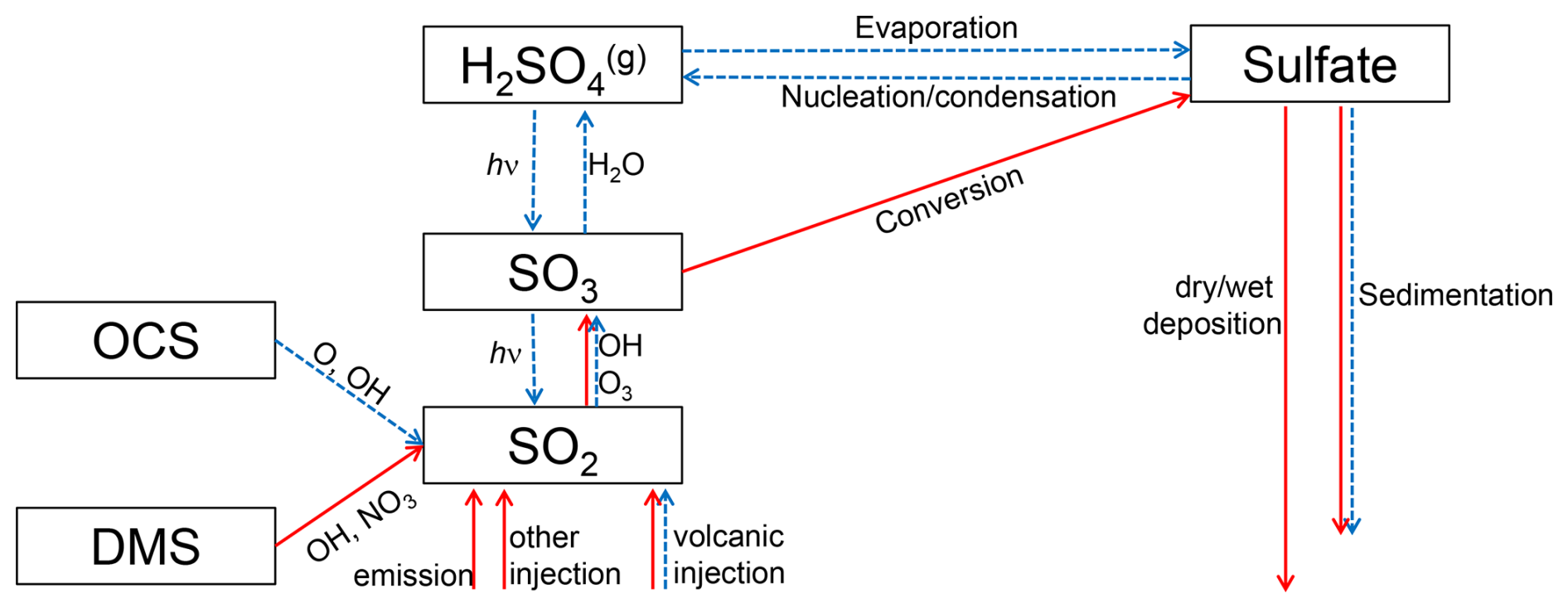
Figure 1 Architecture of the stratospheric sulphur cycle of IFS-COMPO as implemented in Cy49R2. Processes may be activated in the troposphere (red arrows), in the stratosphere (dashed blue arrows) or in the whole column (double arrows).

The production of particulate sulfate in the stratosphere, which represents the combined effect of homogeneous nucleation and condensation, is parameterized as a function of the temperature and concentration of gaseous H₂SO₄. The production rate of aqueous sulfuric acid in s⁻¹ is expressed as:

$$\begin{array}{}\text{(1)}& \mathit{\tau }=a[{\mathrm{H}}_{\mathrm{2}}{\mathrm{SO}}_{\mathrm{4}}{]}_{\mathrm{g}}^b\end{array}$$

where [H₂SO₄]_g is the mass density of gas-phase H₂SO₄ (kg m⁻³), a and b are two constants with values of $\mathrm{5}\times {\mathrm{10}}^{-\mathrm{12}}$ and 2 respectively. The production only occurs if the simulated partial pressure of gaseous H₂SO₄ is above the saturation pressure. The saturation pressure is computed as a function of temperature, pressure and humidity following Ayers et al. (1980) and Kulmala and Laaksonen (1990).

Whenever the partial pressure of gaseous H₂SO₄ is below the saturation pressure, all liquid particles evaporate. The production rate τ is then used to compute the updated mass mixing ratio of gaseous H₂SO₄ from nucleation/condensation:

$$\begin{array}{}\text{(2)}& [{\mathrm{H}}_{\mathrm{2}}{\mathrm{SO}}_{\mathrm{4}}{]}_{\mathrm{g},\text{upd}}=c[{\mathrm{H}}_{\mathrm{2}}{\mathrm{SO}}_{\mathrm{4}}{]}_{\mathrm{g}}{\mathrm{e}}^{-\mathit{\tau }\mathit{\delta }t}\end{array}$$

where δt is the model time step and c is an adjustable parameter (see below). The tendencies of gaseous and particulate H₂SO₄ are derived from the updated mass mixing ratio of gaseous sulphuric acid. The sedimentation of sulfate particles has been adapted to use the sedimentation velocity computed from the Stokes formula rather than adopting fixed sedimentation velocities as done in IFS-COMPO Cy48R1 (for all aerosol species except sea-salt).

The assumed size distribution used to compute the sedimentation velocity is now a simulated variable, depending on the simulated concentration of particulate H₂SO₄. This implicitly represents the more intense coagulation of smaller particles into more coarse modes that typically occurs in volcanic plumes with higher particulate sulfate concentration, resulting in an aerosol size distribution that is more tilted towards coarser particles than in quiescent conditions (Deshler et al., 2003, 2019). The assumed mass median diameter used to compute the sedimentation velocity is computed as:

$$\begin{array}{}\text{(3)}& D=D_{\mathrm{0}}\left(\right[{\mathrm{H}}_{\mathrm{2}}{\mathrm{SO}}_{\mathrm{4}}{]}_{\mathrm{p}}/c{)}^d\end{array}$$

where D₀ is the sulfate wet diameter as computed from the sulfate dry diameter of 0.8 µm and the sulfate hydrophilic growth factor, and [H₂SO₄]_p is the mass density of condensed H₂SO₄ (kg m⁻³). The parameters c and d have been adjusted to $\mathrm{5}\times {\mathrm{10}}^{-\mathrm{8}}$ and 0.25, respectively, to obtain a good agreement with the observed modal diameter of the aerosol size distribution in quiescent and volcanic conditions, as provided by Deshler et al. (2003).

The assumed reference size distribution is representative of the volcanic conditions, where the mechanism lowers the mass median diameter during more quiescent conditions, where the simulated concentration of particulate sulfate is lower, as illustrated in Fig. 2. The simulated wet diameter shows values of between 0.6–0.8 µm in the simulated volcanic plume on 31 January 1992, while the values are typically in the range 0.2–0.3 µm for quiescent conditions, as simulated on 31 January 1998.

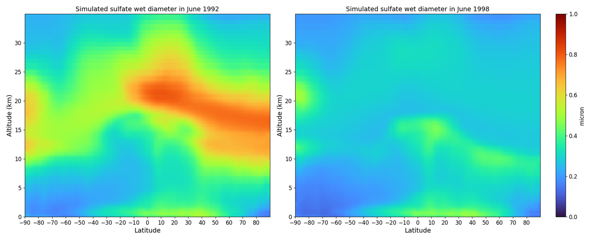
Figure 2 Altitude-latitude monthly-mean cross sections of sulfate wet diameter (µm) as simulated by IFS-COMPO Cy49R1 in June 1992 (left, representative of volcanic conditions), and June 1998 (right, representative of quiescent conditions).

Volcanic injection was further refined in IFS-COMPO Cy49R2, allowing injection over areas that comprise multiple grid cells and enabling the injection of water vapour alongside volcanic sulphur dioxide. These enhancements support the modelling of the impacts of the Pinatubo (1991) and Hunga (2022) eruptions, respectively. Despite these updates the coupling between stratospheric aerosols and chemistry is still not complete in IFS-COMPO Cy49R2, as the information from prognostic stratospheric aerosols is not used in stratospheric heterogeneous chemistry nor are their subsequent AOD values used in the calculation of photolysis rates. Furthermore, wildfire aerosols do not lead to chlorine activation as the model ignores the enhanced solubility of HCl on organic aerosols, and the subsequent heterogeneous reactions of HCl (Solomon et al., 2023). We aim to address these shortcomings in a future development phase of CAMS.

3 Reference datasets

3.1 Aerosols

The Global Space-based Stratospheric Aerosol Climatology (GloSSAC v1.1, Thomason et al., 2018; GloSSAC v2.0, Kovilakam et al., 2020) provides a gap-free monthly-varying global dataset depending on latitude and altitude, for the stratospheric aerosol layer's spatio-temporal variation for the period 1979–2018. It combines several satellite measurement datasets of the stratospheric aerosol layer with ground-based and aircraft-borne lidar measurements, in an attempt to fill gaps in the satellite measurements which occurred around the 1982 El Chichon eruption (gap between SAGE and SAGE-II) and after the 1991 Pinatubo eruption (see below) using a methodology detailed by SPARC (2006, chapter 4). The latest version, GloSSAC v2.2, ends in 2021 (NASA/LARC/SD/ASDC, 2022).

The GloSSAC dataset provides monthly-mean profiles of the aerosol extinction at wavelength 525 nm, on a vertical grid with 0.5 km spacing and a latitude grid with 5° intervals ranging from 77.5° S to 77.5° N. It also provides, on the same latitude grid, monthly-mean stratospheric Aerosol Optical Depths (AOD) which are vertically integrated from the tropopause up to 40 km altitude and additional “derived products” including stratospheric aerosol Surface Area Density (SAD), stratospheric aerosol volume concentration and stratospheric aerosol effective radius. However, the SAD is available only in GloSSAC v1.1 and not in v2.0 nor in v2.2. For the Pinatubo simulation (1991–1993) described at Sect. 4.3 and evaluated at Sect. 8, GloSSAC is based almost entirely on the measurements from the SAGE-II solar occultation instrument which provided observations up to September 2005. However the large opacity of the volcanic cloud injected by the Pinatubo eruption rendered the optical signal too weak for the sensitivity of SAGE-II, during several months, making the estimation of the aerosol burden very uncertain for this period. In consequence, the GloSSAC data have to be considered very cautiously for some months after June 1991, and we indeed notice that the stratospheric sulfate burden and AOD derived in GloSSAC are still underestimated in the domain of the volcanic plume (40° S–40° N latitude) for 1–1.5 years after the June 1991 Pinatubo eruption.

Since the saturation issue of SAGE-II after the Pinatubo is not entirely corrected in GloSSAC, we use two other satellite datasets in our evaluation. First we use the stratospheric AOD retrieved retrieved by Quaglia et al. (2023) from the Advanced Very High Resolution Radiometer (AVHRR/2), a space-borne sensor which measured the reflectance of the Earth in five spectral bands covering visible and infrared wavelengths (0.63, 0.86, 3.7, 11, 12 µm). The AVHRR/2 instrument, on board the polar-orbiting satellites (POES) NOAA-11, provided global coverage data twice per day with a resolution of 1.1 km. AVHRR cannot detect variations in stratospheric AOD smaller than 0.01, but can detect values up to 2.0 (Russell et al., 1996).

Second, we use the total particulate sulfate burden derived from High resolution Infra Red Sounder (HIRS) observations (Baran and Foot, 1994). While the limb-occultation measurements of SAGE-II provide vertical aerosol profiles and hence distinguish between tropospheric and stratospheric aerosols when the aerosol load in low enough, HIRS observes the nadir aerosol vertical column and derives the total (i.e. tropospheric + stratospheric) aerosol mass with about 10 % uncertainties. During the first year after the Pinatubo eruption, the aerosol burden derived from SAGE-II is noticeably lower than the burden derived from HIRS observation. This disagreement is likely related to the saturation effects of SAGE-II as a limb-occultation instrument during this period (Russell et al., 1996). The SAGE-3λ composite (Feinberg et al., 2019) provides significantly larger burdens than its predecessor (Arfeuille et al., 2013) due to additional data used in a gap-filling procedure (Revell et al., 2017), but is still much lower than HIRS. SAGE-II provides altitude-resolved extinction profiles, while HIRS estimates vertically-integrated aerosol mass. Over time, SAGE-II measurements are expected to yield more accurate aerosol extinction values, and therefore, more precise estimates of stratospheric sulfate mass. This improvement becomes evident once the atmosphere becomes sufficiently transparent. In contrast, HIRS-derived aerosol mass estimates become less reliable as the aerosol cloud spreads to higher latitudes. At these latitudes, the values approach the noise level of the HIRS technique, reducing its accuracy (Baran and Foot, 1994). This suggests that the HIRS data should be trusted until mid-1992 and the SAGE data afterwards, as suggested by Sheng et al. (2015).

The Stratospheric Aerosol and Gas Experiment on the International Space Station (SAGE III/ISS) works similar to its predecessors SAGE and SAGE-II and observes the aerosol extinction coefficients at nine different wavelengths in the UV-visible-IR range between 384 and 1545 nm (Mauldin et al., 1985; Cisewski et al., 2014). IFS-COMPO provides 3D output of simulated aerosol extinction at wavelengths 355, 532 and 1064 nm, which are compared in Sect. 5.7 against the closest available wavelengths (i.e. 384, 521 and 1022 nm) from the SAGE III/ISS v5.3 data (NASA/LARC/SD/ASDC, 2025).

3.2 Retrievals of gas-phase species

The primary target of CAMS in the stratosphere is the concentration of O₃ which is mostly determined by the Chapman cycle and four catalytic destruction cycles with the NO_x (NO+NO₂), HO_x ($\mathrm{H}+\mathrm{OH}+{\mathrm{HO}}_{\mathrm{2}}$), ClO_x (Cl+ClO), and BrO_x (Br+BrO) families (Brasseur and Solomon, 2005). A comprehensive evaluation should use vertically resolved measurements of the concentrations of one member for each family, as well as their long-lived source or reservoir species. These measurements are available from limb-scanning satellite instruments, except for BrO_x members where we use a ground-based spectrometer (see below) and HO_x members which are not measured in the lower and middle stratosphere.

The global evaluation relies on retrievals from the Atmospheric Chemistry Experiment Fourier Transform Spectrometer (ACE-FTS) onboard the Canadian satellite SCISAT and from the Microwave Limb Sounder onboard NASA's Aura satellite (Aura-MLS). Operating continuously since February 2004, ACE-FTS observes up to 30 solar occultation (sunrise and sunset) events every day, with a higher density in the high latitudes than in the Tropics and with a vertical resolution of about 3 km from an altitude of 5 km (or the cloud tops) up to 150 km (Bernath, 2017). We use the retrievals of 11 gas-phase species (N₂O, H₂O, NO, NO₂, HCl, HNO₃, ClO, CH₄, ClONO₂, N₂O₅ and O₃) among the 46 available in ACE-FTS version 5.2 (Boone et al., 2023). The ACE-FTS used here are screened using the ACE-FTS data quality flags (Sheese and Walker, 2025). As in Errera et al. (2019), the screening approach is modified from Sheese et al. (2015) in order to de-flag events which may have been erroneously identified as outliers (e.g. Sheese et al., 2017).

Aura-MLS is operating continuously since August 2004 and delivers around 3500 vertical profiles every day, during daytime as well as night-time. We use the Level 2 retrievals of 6 gas-phase species (N₂O, H₂O, HCl, HNO₃, ClO and O₃) in Aura-MLS version 5.0 (NASA GES DISC, 2025). As recommended in the corresponding data quality and description document (Livesey et al., 2022), the retrieved profiles which do not satisfy the recommended criteria for estimated precision, quality, convergence or status are filtered out while retaining negative values to avoid any overestimation of the mean profiles. In particular, this screening discards profiles contaminated by clouds, mainly for O₃ and HNO₃. The biases in ClO profiles at and below 68 hPa have been corrected as recommended by Livesey et al. (2022). Sheese et al. (2017) compared Aura-MLS retrievals v3.3 and ACE-FTS v3.6 retrievals for O₃, N₂O, H₂O and HNO₃, indicating typical agreements better than ±10 % below 35 km altitude, except for the N₂O retrievals. N₂O is a special concern in Aura-MLS retrievals because two different products are available: the standard product, retrieved from radiance observations in the 190 GHz region, suffers from a significant underestimation reaching up to 20 % below 35 km altitude (Sheese et al., 2017); and an alternate product, retrieved from the more favorable 640 GHz region, but not usable after 7 June 2013 (Livesey et al., 2022).

While the ACE-FTS and Aura-MLS datasets include two intermediate reservoirs for chlorine (HCl and ClONO₂) and a chlorine radical participating in the catalytic destruction of ozone (ClO), they do not include any usable bromine species. Aura-MLS v5.0 does include BrO retrievals, but these should not be used below 10 hPa (Livesey et al., 2022) while we are primarily interested in ozone depletion processes in the lower stratosphere.

Many UV-Vis spectrometers allow retrieval of the total BrO column, from the ground and from satellites, but the tropospheric contribution to this column may be significant in the polar regions (see e.g. Chen et al., 2023) while BrO is currently not represented in the tropospheric chemistry module CB05. The ground-based instrument in Harestua (60.2° N, 10.8° E) has sufficiently good observations to allow separation of the tropospheric and stratospheric BrO column densities by the DOAS technique (Hendrick et al., 2009). The corresponding product is converted from slant column density to vertical column density by application of appropriate Air Mass Factors, and the values at 13.5 h (solar local time) are derived from the sunrise/sunset measurements using an offline box-model. The final ground-based product can thus be compared in a straightforward manner with BrO total columns by IFS-COMPO at noon UT.

The Michelson Interferometer for Passive Atmospheric Sounding instrument (MIPAS), onboard the Envisat satellite, recorded atmospheric infrared spectra from 2002 until 2012 (Fischer et al., 2008). To evaluate the night-time abundance of BrONO₂ in the polar regions, we use a monthly-mean dataset derived from MIPAS retrievals (Höpfner et al., 2021). The measured spectra were filtered out to remove both tropospheric and polar stratospheric clouds. The BrONO₂ spectra were binned in 18 latitude bands with 10° spacing and with a temporal binning of 3 d. The vertical resolution is approximately 3 km at 15 km and decreases with altitude, reaching 8 km at 35 km of altitude.

3.3 Updated BASCOE reanalyses of Aura-MLS and MIPAS

Reanalyses of chemical composition allow the initialization of chemical forecast experiments, and the evaluation of the results of these forecasts through simple comparisons with the initializing reanalysis. This is the approach adopted for the initialization and evaluation of the seven polar winter-spring experiments realized with IFS-COMPO Cy49R1 (see Sect. 4.2 below). To this aim we use the BASCOE Reanalysis of Aura MLS, version 3 (BRAM3), an upgrade of BRAM2 (Errera et al., 2019). Both reanalyses result from the assimilation of Aura-MLS v4.2 observations of O₃, N₂O, H₂O, HNO₃, HCl, CO, CH₃Cl and ClO (Livesey et al., 2015) by the BASCOE chemical Data Assimilation System (DAS), but with different configurations (see Table 1). The most notable difference is the extension of the covered period until November 2023, thanks to the replacement of the input reanalysis for dynamical fields, from ERA-Interim (Dee et al., 2011) in BRAM2 to ERA5 (Hersbach et al., 2017, 2020) in BRAM3.

Table 1 Differences between the configurations of the BASCOE chemical Data Assimilation System (DAS) used for the BRAM2 reanalysis (Errera et al., 2019) and the upgraded version BRAM3.

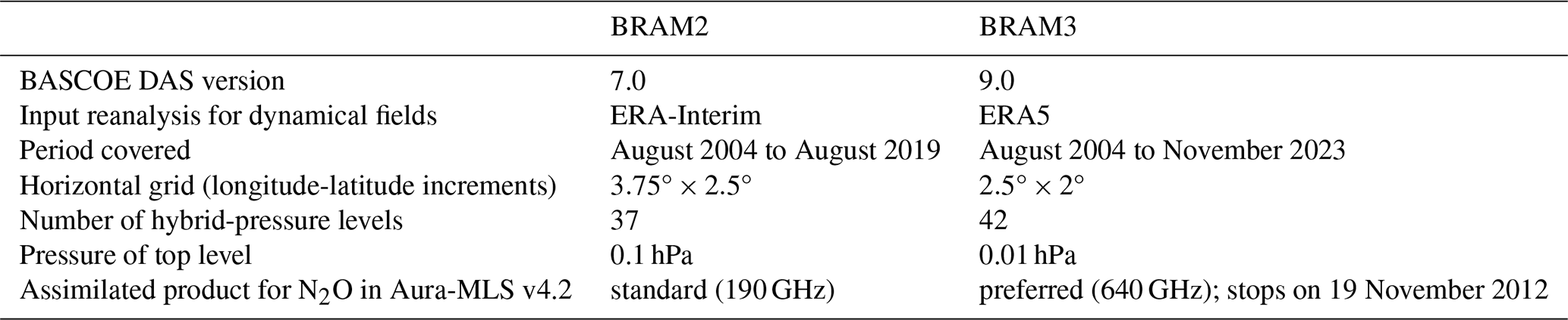
Another notable difference is the specific N₂O product which was assimilated from the Aura-MLS v4.2 dataset. The product assimilated into BRAM2 was the standard 190 GHz product which suffers from a low bias (see above) but is available for the whole duration of the mission. A drift was detected in the BRAM2 reanalysis of N₂O (Errera et al., 2019) and attributed to instrumental degradation of this spectrometer (Livesey et al., 2021). The alternate product, retrieved from the 640 GHz spectrometer, was assimilated into BRAM3 only until 19 November 2012. On later dates, the N₂O output of BRAM3 is not constrained by any observations.

BRAM3 was evaluated in the same manner as BRAM2 (Errera et al., 2019), i.e. through comparisons of the assimilated species with the Aura-MLS v4.2 input observations, with ACE-FTS v3.6 retrievals (Sheese et al., 2017), and with MIPAS retrievals (von Clarmann et al., 2013). The mean biases and standard deviations of the differences are as good or better than those obtained with BRAM2.

The evaluation of NO₂ in the polar regions (in Sect. 6.4 below) relies on MIPAS observations through another updated reanalysis by the BASCOE DAS. The first BASCOE analysis assimilated MIPAS NO₂ retrievals v4.61 (Wetzel et al., 2007) with a 4D-VAR algorithm (Errera et al., 2008). We use here a reanalysis of the MIPAS NO₂ retrievals v6 (Raspollini et al., 2013) generated by an upgraded 4D-VAR configuration of the BASCOE DAS (Errera et al., 2016). This reanalysis, labelled REAN01, was validated in the same manner as an earlier analysis of MIPAS O₃ retrievals (Errera and Ménard, 2012) and delivered mean biases and standard deviations of the differences which are as good or better than those obtained with the original analysis of MIPAS NO₂ (Errera et al., 2008).

4 Setting up the modelling experiments

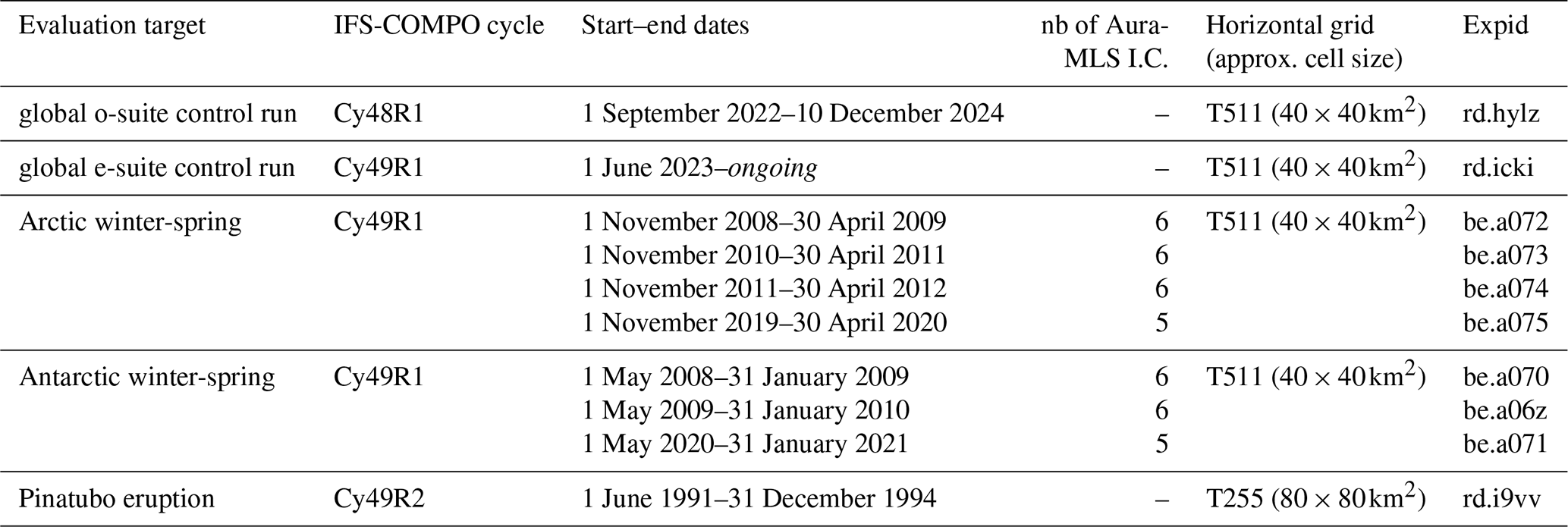
As explained in Sect. 1, IFS-COMPO Cy49 is too computationally expensive to run the long simulation required for climatological evaluation. As summarized by Table 2, we focus instead on three separate case studies with IFS-COMPO experiments lasting 6 to 24 months. These case studies have been chosen to exemplify the performance of Cy49 during both exceptional and quiescent meteorological conditions namely: (i) global statistics during a recent period preparing for the upgrade of the operational service; (ii) ozone depletion processes in the polar regions for various years and the (iii) the Pinatubo eruption in 1991 as a test of the capacity to simulate sulfate aerosol distributions in the stratosphere after exceptionally large volcanic injections of SO₂. In this section, we provide some details about the setup of the model for these modelling experiments.

Table 2 Details of the IFS-COMPO modelling experiments evaluated by comparison with observations or chemical reanalyses. The 4th column indicates the number of species initialised from Aura-MLS observations through the BRAM3 reanalysis (see Sect. 4.3).

4.1 Case study 1: o-suite and e-suite control runs

The operational analyses and forecasts of global atmospheric composition delivered by CAMS were upgraded from IFS-COMPO Cy48R1 to Cy49R1 on 12 November 2024. This operational process, named “o-suite”, simultaneously assimilates meteorological observations (the same observations as assimilated for NWP analyses) and composition observations. The assimilated composition observations include total ozone columns, vertical ozone profiles and Aerosol Optical Depths (AOD) which constrain the model results in the stratosphere (Eskes et al., 2024a). The candidate for the next system upgrade is run in parallel with the o-suite and is named “e-suite”. Eskes et al. (2024b) evaluate the e-suite for the CAMS Cy49R1 upgrade of 12 November 2024.

Here we aim to evaluate chemical forecast experiments that last a few months to a few years (see Table 2) and are constrained by the assimilation of meteorological observations while there is no assimilation of composition observations. In the context of CAMS operations, this is enabled by the “control runs” which are run in parallel with operational processes with the dynamical fields re-initialised every day from the corresponding analyses while the composition fields are not constrained by any observations of atmospheric composition. In Sect. 5, we thus evaluate the Cy49R1 upgrade by comparing the Cy48R1 (o-suite) control run, labelled rd.hylz, with the corresponding Cy49R1 (e-suite) control run, labelled rd.icki. These two control runs do not account for the large masses of H₂O and SO₂ which were injected into the stratosphere by the explosive eruption of the Hunga volcano on 15 January 2022 (Li et al., 2024; Fleming et al., 2024). These aspects are addressed specifically through the participation of IFS-COMPO Cy49R1 to the Hunga model-observation comparison (Zhu et al., 2025).

The initial composition of the e-suite control run on 1 June 2023 is read in from the o-suite control run on that date. The initial composition of the o-suite control run on 1 September 2022 is the outcome of a series of preliminary experiments with preparatory versions of IFS-COMPO Cy48R1, starting on 1 July 2013 from the BRAM2 reanalysis (Errera et al., 2019). IFS-COMPO was thus spinned up during 10 years before this test case, i.e. for a longer time than the largest mean Age of Air encountered in the stratosphere (Chabrillat et al., 2018).

4.2 Case Study 2: Winter-spring seasons in the polar regions

The fundamental connections between chlorofluorocarbon emissions, heterogeneous chemistry on stratospheric particles, and O₃ depletion have been clear for decades (Solomon, 1999; Solomon et al., 2015), and the monitoring of polar O₃ depletion events is arguably the most important application of CAMS with respect to stratospheric composition (Lefever et al., 2015; Inness et al., 2020). In this work we aim to evaluate the ability of IFS-COMPO Cy49R1 to forecast the composition of the lower stratosphere at the poles during the winter where chemical pre-processing occurs in the polar vortex, and during the springtime return of sunlight and the associated ozone depletion.

Since polar O₃ depletion is subject to interannual variability in meteorology, the evaluation is realized over three winter-spring seasons above the Antarctic and four winter-spring seasons above the Arctic. Figure 3 illustrates this variability through the evolution of temperature and O₃ above the poles for the selected years: 2008, 2009 and 2020 for the Antarctic and 2008–2009, 2010–2011, 2011–2012, 2019–2020 for the Arctic.

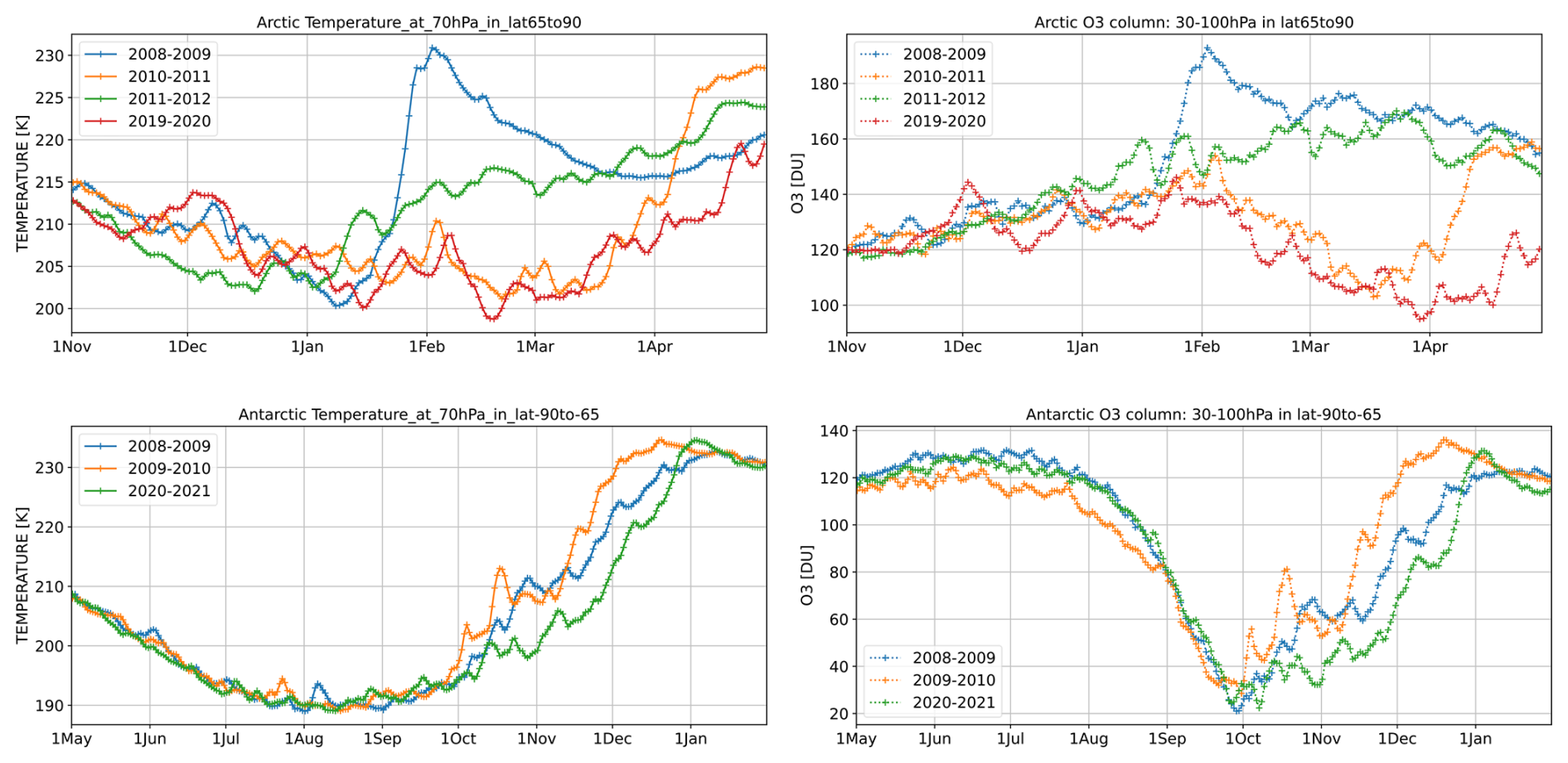
Figure 3 Mean ERA5 temperature at 70 hPa (left) and BRAM3 reanalyses of the O₃ partial columns (30–100 hPa, right) above the Arctic (65–90° N, top) for the winter-spring seasons of 2008–2009 (blue), 2010–2011 (orange), 2011–2012 (green) and 2019–2020 (red) and above the Antarctic (90–65° S, bottom) for the winter-spring seasons of 2008 (blue), 2009 (orange) and 2020 (green).

The large and long-lasting Antarctic O₃ hole of 2008 has been studied extensively with both forecast and analysis experiments by the first configurations of IFS-COMPO as developed for MACC (Flemming et al., 2011). While the Antarctic O₃ hole of 2009 had a similar volume of Southern Hemisphere air below the condensation temperature of ice PSC (VPSC: Lawrence et al., 2015), Fig. 3 shows a Sudden Stratospheric Warming (SSW) on mid-October 2009, accompanied by a temporary peak of O₃. Model biases until the end of September 2009 should thus be quite similar to those for 2008, allowing a consistency check for the first part of the season, and noticeable differences between 2008 and 2009 should arise for the second part of the season.

The Antarctic O₃ hole of 2020 also had a very large size, and it lasted longer than any previously observed Antarctic O₃ hole since 1980 (Stone et al., 2021). This corresponds with low temperatures lasting much longer than in 2008: the dynamical evolution of the vortex in 2020 was clearly exceptional, and it is tempting to draw causal links with the exceptional injection of aerosol by the Australian bushfires which happened earlier that year (Tencé et al., 2022). Salawitch and McBride (2022) reviewed such possible feedbacks between dynamics, aerosols and chemistry. It is an interesting question how IFS-COMPO forecasts this O₃ hole episode with constrained dynamics but no representation of wildfire-related aerosols in the stratosphere.

Figure 3 also presents the ERA5 temperatures above the Arctic (65–90° N; right panels) during four winter-spring seasons ending in 2009, 2011, 2012 and 2020. In 2008–2009 a major Sudden Stratospheric Warming (SSW) increased temperature by 30 K in mid-January accompanied with an increase of O₃ during the two next weeks. In 2010–2011 the temperatures and O₃ columns kept decreasing until the end of March, indicating an exceptional O₃ depletion event (see e.g. Manney et al., 2011; Strahan et al., 2013) which was studied extensively with both the MACC and CAMS analyses (Lefever et al., 2015; Inness et al., 2020). This is clearly an important event to assess the forecasting abilities of IFS-COMPO. The 2011–2012 season seems quite uneventful by comparison, with temperatures decreasing until December 2011 followed by a slow warming. This can thus be considered as a typical Arctic episode. The 2019–2020 season was very similar to 2010–2011, with an exceptionally strong and stable polar vortex causing again sustained low temperatures and a record-breaking O₃ hole event, which was already compared with the 2011 event through CAMS analyses (Inness et al., 2020).

The seven polar winter-spring experiments use the same horizontal and vertical grids as the o-suite and e-suite control runs and a similar “cycling forecast” configuration, with the meteorological initial conditions of each 24 h cycle taken from the ERA5 reanalysis, while the composition fields remain unconstrained. For each experiment, atmospheric composition is initialised on 1 November (for Arctic evaluation experiments) or on 1 May (for Antarctic evaluation experiments) by combining an earlier IFS-COMPO experiment for tropospheric levels with the BRAM3 reanalysis for stratospheric levels (see Sect. 3.3). This is a fundamental difference with the control runs, which have not been constrained by any assimilation of composition data for the 10 previous years. In this case study, at least five species (H₂O, HCl, HNO₃, ClO and O₃) are initialized from Aura-MLS through BRAM3, as well as N₂O for the experiments which start before 2012, i.e. before BRAM3 stopped assimilating Aura-MLS N₂O.

The initial conditions of these seven experiments are available (Chabrillat and Errera, 2025) for reproduction of the chemical forecasts with other models of stratospheric composition. Their evaluation, in Sect. 6 below, rests primarily on comparisons with the daily zonal means of the 6 species assimilated in BRAM3. These BRAM3 daily zonal means are also made available (Errera and Chabrillat, 2025) for reproduction of this evaluation

4.3 Case study 3: Pinatubo eruption

The first application of the stratospheric aerosol extension in IFS-COMPO Cy49R2 is a simulation of the evolution of the global volcanic aerosol cloud that formed in the stratosphere from the tropical eruption of Mount Pinatubo in the Philippines in June 1991. With a volcanic explosivity index of 6 and a dust veil index of 1000, this was the most important eruption since the Krakatau eruption in 1883, and the first major eruption cloud whose evolving stratospheric aerosol characteristics and subsequent dispersion to both hemispheres could be fully observed by satellite sounders (Robock, 2000). The Pinatubo eruptions has already been the subject of numerous simulations (e.g. Dhomse et al., 2014; Sheng et al., 2015; Mills et al., 2016; Kleinschmitt et al., 2017; Sukhodolov et al., 2018; Hu et al., 2025) and represents a good benchmark to evaluate the newly added stratospheric aerosol component of IFS-COMPO Cy49.

As in the chemical forecast experiments for evaluation of polar winter-spring seasons, the Pinatubo eruption experiment is configured as a “cycling forecast” using the ERA5 reanalysis to constrain the meteorological fields every 24 h while no data assimilation of aerosols and chemistry is used. Lasting more than two years, this experiment would be too costly to run at the T511 resolution currently used for CAMS. Hence the T255 resolution, corresponding to an 80 km grid cell, was selected instead. For the Pinatubo eruption, a total of 14 Tg of SO₂ was injected on 15 June 1991 between 18 and 24 km altitude (Sukhodolov et al., 2018). To better take into account the explosive nature of the eruption and local dynamical processes not described by the model, the injection was distributed over a 300 km×300 km area centered on the Pinatubo. The additional impact of the Cerro Hudson eruption is captured by also injecting 2.3 Tg of SO₂ on 15 August 1991, over a 300 km×300 km area centered on the Cerro Hudson.

5 Global evaluation: July 2023 to May 2024

In this section we evaluate and discuss the distributions of ten gas-phase species, and of the aerosol extinction coefficients, as simulated by IFS-COMPO Cy48R1 and Cy49R1, through comparisons with ACE-FTS, Aura-MLS, and SAGE III/ISS in the case of aerosols. The comparison methodology is built on the validation tools developed for the evaluations of stratospheric gases in the operational analyses and short-term forecasts of the CAMS global service which are published every three months (most lately by Errera et al., 2024) and with every system upgrade (Eskes et al., 2024b). These evaluations include mean values and statistics of the differences between the simulations and the retrievals, over a period of 11 months starting on 1 July 2023 and ending on 31 May 2024. Prior to computation of the statistics, the model output was retrieved with a time resolution of three hours and interpolated to the location and time of each retrieved profile. N₂O is evaluated in Sect. 5.1 as an example of long-lived tracer. H₂O is evaluated in Sect. 5.2. In Sect. 5.3 we evaluate HCl and three other gases impacted by heterogeneous chemistry. Sections 5.4, 5.5 and 5.6 discuss ClO, nitrogen oxides and O₃, respectively. Finally, Sect. 5.7 shows the first stratospheric aerosol results by IFS-COMPO. For the sake of conciseness, evaluation figures are presented for only six species (N₂O, H₂O, HCl, NO_x, ClO, O₃) while the Supplement includes evaluation figures of four other species (CH₄, HNO₃, ClONO₂, N₂O₅).

5.1 N₂O and CH₄

N₂O (Fig. 4) is a long-lived “source” tracer, i.e. it is emitted at the surface and destroyed in the stratosphere (Brasseur and Solomon, 2005). A vertical discontinuity between the pressure levels at 10 and 30 hPa is easily seen in the Aura-MLS observations, reflecting instrumental issues in the standard 190 Ghz product available for this period (see Sects. 3.2 and 3.3). The N₂O biases between IFS-COMPO and Aura-MLS should thus be discarded. A much better agreement is obtained with ACE-FTS below 10 hPa, where the biases and standard deviations are smaller than 10 % and the correlations remain above 0.8 except for the lowermost levels. Furthermore the biases with respect to ACE-FTS are noticeably smaller with the upgraded IFS-COMPO Cy49R1 than with Cy48R1. Since the photochemistry of N₂O did not change between Cy48R1 and Cy49R1, this can be attributed to the activation of the Bermejo–Conde mass fixer in the transport module (see Sect. 2.2).

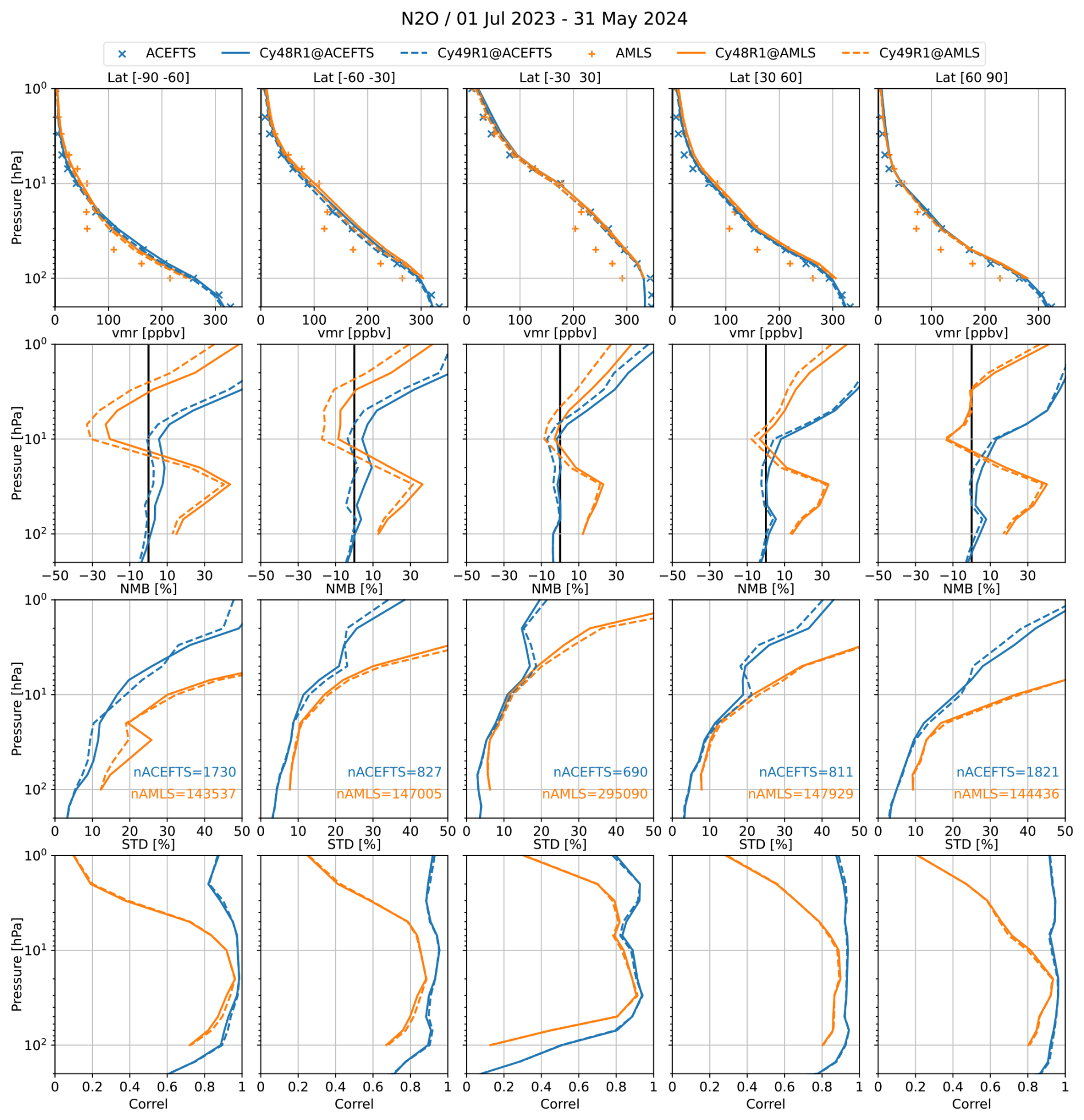
Figure 4 Comparison of N₂O simulated in the IFS-COMPO control runs Cy48R1 (solid lines) and Cy49R1 (dashed lines) with MLS (orange) and ACE-FTS (blue) profile observations between July 2023 and May 2024. Statistics are segregated into five latitude bands spanning both the Southern and Northern Hemispheres, from left to right: 90–60° S, 60–30° S, 30° S–30° N, 30–60° N and 60–90° N. Statistical values shown are, from top to bottom: mean volume mixing ratio (vmr); mean bias (model minus observations) normalized by the mean of the model profile (NMB); standard deviation of the mean bias (STD); and the correlation between models and observations (Correl). The number of profiles used in each comparison are given in the third (STD) row.

In the upper stratosphere, i.e. at pressures lower than 10 hPa, the N₂O biases between IFS-COMPO and ACE-FTS increase quickly to reach or exceed 50 % at the upper limit of our evaluation (1 hPa pressure level). Similar biases are obtained with CH₄ (Fig. S2 in the Supplement) and CFC-12 (not shown), and also with the experiments designed to study past winter-spring polar seasons with dynamical fields from ERA5 (not shown). Since the uppermost model level is at 0.01 hPa pressure, i.e. in the mesosphere and approximately 30 km above the upper limit of our evaluation, the upper boundary condition is not expected to play a role in this disagreement. This suggests that a common process leads to the overestimation of all source tracers in the upper stratosphere, and it is tempting to identify this process with the Brewer–Dobson Circulation (BDC; see the review by Butchart, 2014). A misrepresentation of the wind fields in the meteorological analyses at pressures lower 10 hPa could lead to excessively strong vertical transport in the deep tropical branch of the BDC, resulting in too young mean Age of Air (AoA; see the review by Waugh and Hall, 2002). Earlier comparisons between IFS-COMPO N₂O and CH₄ and ACE-FTS retrievals above 10 hPa had an opposite outcome, i.e. a model underestimation (Huijnen et al., 2016). This change of sign in upper stratospheric biases could lend support to our hypothesis, because Huijnen et al. (2016) used winds by ERA-Interim which produce a different BDC than the ERA5 winds or the winds used here. Yet Chemistry-Transport Models (CTM) seem to invalidate this hypothesis, at least below 10 hPa, as the BASCOE CTM driven by ERA-Interim yields an AoA in good agreement with in-situ observations up to 8 hPa in the Tropics (Chabrillat et al., 2018), and another CTM-based study indicates that the AoA derived from ERA5 is older – not younger – than the AoA derived from ERA-Interim, at all latitudes (Ploeger et al., 2021). One must note though that this comparison of AoA with ERA-Interim and AoA with ERA5 (Ploeger et al., 2021) does not extend above the 800 K potential temperature (or approximately 10 hPa) level.

These AoA modelling studies do not reach high enough into the stratosphere to clearly confirm or disprove an overestimation of the BDC strength in the IFS (re-)analyses, because observational evidence in this region is scarce. Most observational derivations of AoA do not reach into the upper stratosphere (e.g., Engel et al., 2017; Saunders et al., 2025). The AoA dataset derived from MIPAS SF₆ retrievals does reach 50 km, i.e. approximately 1 hPa (Haenel et al., 2015; updated by Stiller et al., 2021). Further research is clearly warranted, either by comparisons between the MIPAS AoA dataset and IFS simulations of AoA (e.g. using a clock tracer) or through implementation of SF₆ into the BASCOE module of IFS-COMPO.

5.2  H₂O

A chemical H₂O trace gas is defined at all levels within the composition component of IFS-COMPO. In the troposphere, the H₂O mass mixing ratios are constrained by the humidity (q). This humidity is simulated in the meteorological component (IFS) and acts at the tropopause as a boundary condition for water vapor in the stratosphere. In the stratosphere, H₂O is governed by chemical production and loss (Huijnen et al., 2016).

The upgrade from Cy48R1 to Cy49R1 has no significant impact on H₂O (Fig. 5). Following the BDC, we first inspect the tropical lower stratosphere, i.e. below 70 hPa. In this region, which is most directly impacted by the boundary condition at the tropopause, IFS-COMPO exhibits a large moist bias with model values larger than observations by more than 50 % at 100 hPa, both with ACE-FTS and Aura-MLS. This issue is a prime target for improvement in future versions of the model.

Figure 5 Same as Fig. 4 but for H₂O.

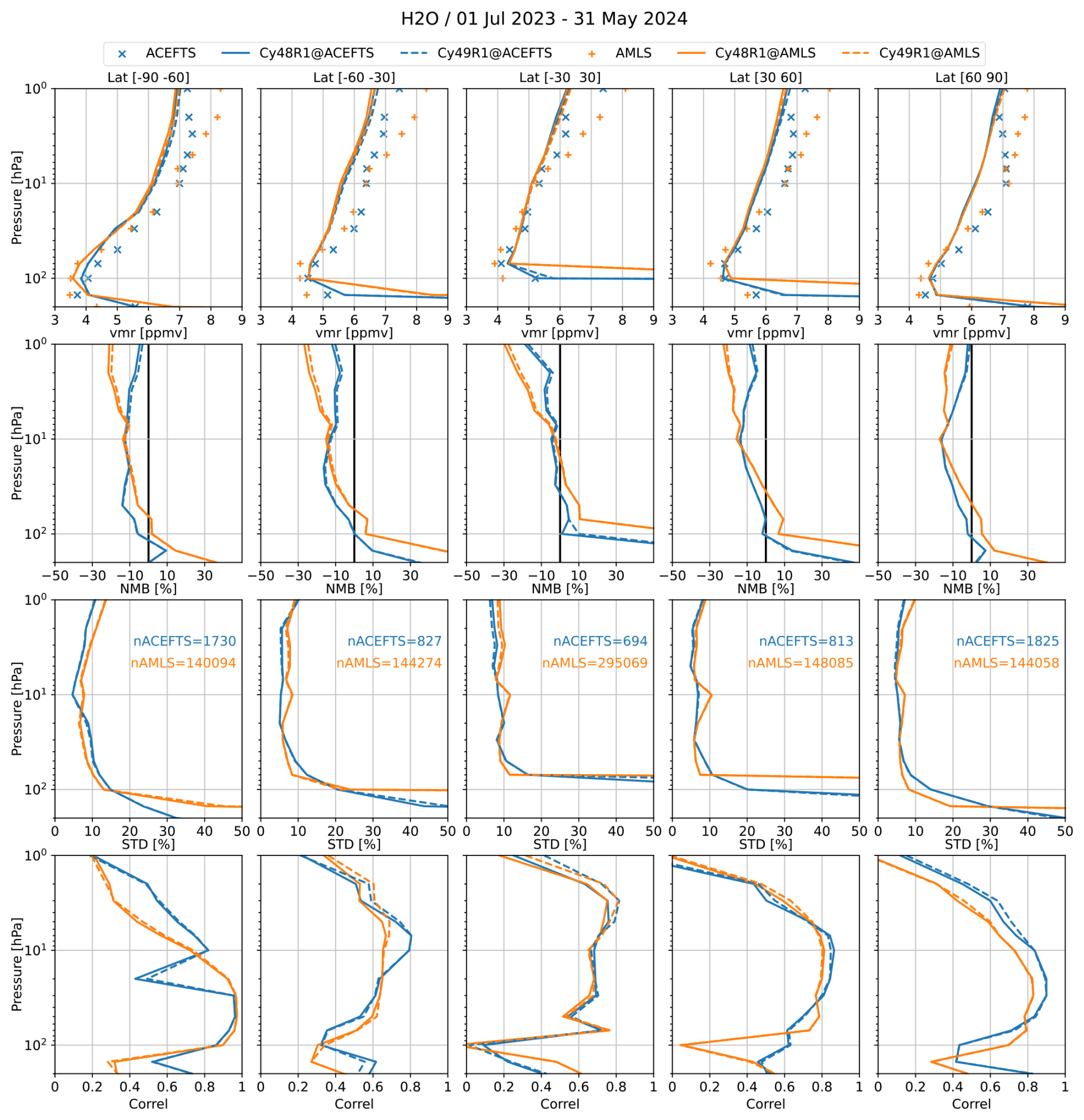
In the tropical middle stratosphere, i.e. between 6 and 50 hPa, the IFS-COMPO biases are smaller than 10 % with respect to Aura-MLS and smaller than 5 % with respect to ACE-FTS, the standard deviations remain below 10 % and the correlations around 0.7. This reflects the good results obtained in the comparison between N₂O and ACE-FTS (Fig. 4), except for smaller correlations with the observations. In the tropical upper stratosphere IFS-COMPO develops a negative bias with decreasing pressures, reaching at 1 hPa underestimations of 15 % with respect to ACE-FTS and 20 % with respect to Aura-MLS. Since water vapour is produced by the oxidation of methane in the upper stratosphere (le Texier et al., 1988), this underestimation is consistent with the hypothesis of an overly strong deep tropical branch of the BDC (see above).

Moving to the extratropics, we also note an underestimation of upper stratospheric H₂O by around 10 % with respect to ACE-FTS and less than 20 % with respect to Aura-MLS, with even smaller biases above the North Pole. The standard deviations of differences between forecasts and observations remain below 5 % at nearly all extratropical levels, except above the South Pole: the next section discusses in more detail H₂O in the polar lower stratosphere. In the extratropical upper stratosphere the correlations between forecasts and observations decrease rapidly with pressure, probably due to the increasing importance of the diurnal cycle: fast variations are poorly sampled in three-hourly IFS-COMPO output.

The H₂O bias with respect to ACE-FTS in the Southern mid-latitudes peaks at 30 hPa, and at this pressure level the H₂O bias is more severe in Southern mid-latitudes than in the other latitude bands. We interpret this as the signal of the 15 January 2022 Hunga eruption, which was not considered in the IFS-COMPO o-suite and e-suite (see Sect. 4.1). No such bias can be observed in the Tropics because water vapour in this region is controlled by tropical tropopause temperatures and the upward branch of the Brewer–Dobson Circulation. In other terms, the impact of the Hunga eruption on stratospheric H₂O cannot be seen in the Tropics after 18 months because it has been erased by the tape recorder effect (Mote et al., 1996; Schoeberl et al., 2012).

Most climate models suffer from large moist biases in the extratropical lowermost stratosphere, i.e. below about 100 hPa, likely due to difficulties modelling transport of water vapor near the tropopause with a strong gradient (Charlesworth et al., 2023). This issue also impacts humidity in the lowermost stratosphere of IFS, contributing to a cold bias in the NWP-oriented configuration (Bland et al., 2024) and explaining the large overestimation shown by Fig. 5 in the mid-latitudes below 100 hPa.

5.3 HCl, HNO₃, ClONO₂ and N₂O₅

HCl is produced by oxidation and photolysis of chlorine-bearing source tracers, most notably the man-made chlorofluorocarbons, resulting in a positive vertical gradient of its volume mixing ratio (vmr) throughout the stratosphere (Brasseur and Solomon, 2005). The global distribution of HCl (top row of Fig. 6) is well captured by IFS-COMPO, including the weaker vertical gradients between approximately 20 and 70 hPa in all latitude bands except for the Arctic. A low bias of approximately 10 % is noted above (i.e. at pressures lower than) 10 hPa, similar to the underestimation found for H₂O and probably sharing the same causes: the discussion about a possible misrepresentation of the BDC applies to HCl as well. The upgrade of heterogeneous chemical rates from IFS-COMPO Cy48R1 to Cy49R1 (see Sect. 2.2) had clearly beneficial impacts on HCl, reducing the biases and the standard deviations and increasing the correlations with observations at most pressure levels below 10 hPa. Large negative biases nonetheless remain in the lower stratosphere with IFS-COMPO Cy49R1, reaching approximately −30 % with respect to ACE-FTS in the mid-latitudes at the 30 hPa pressure level while the corresponding standard deviations are below 15 %.

Figure 6 Same as Fig. 4 but for HCl.

The evaluation of HNO₃ (Fig. S3 in the Supplement) also shows an improvement with the IFS-COMPO cycle upgrade, but HNO₃ remains even more underestimated than HCl in the lower stratosphere while the standard deviations reach very large values (more than 50 % at 70 hPa). ClONO₂ (Fig. S4 in the Supplement) is overestimated by up to 30 % at 100 hPa in the mid-latitudes and more than 60 % below 60 hPa in the Tropics. While normalized biases are less reliable in this region due to the very small observed vmr, the evaluation of N₂O₅ (Fig. S5 in the Supplement) also points to issues with the modelling of heterogeneous chemistry with overestimations reaching 30 % at 30 hPa where standard deviations exceed 20 %, in all latitude bands.

Overall, the disagreements in HCl, HNO₃, ClONO₂ and N₂O₅ indicate not only deficiencies in the representation of heterogeneous chemistry, but also the need for future versions of IFS-COMPO to capture the partitioning of HNO₃ between its gaseous and condensed phases – including its neutralization by semi-volatile cations such as ${\mathrm{NH}}_{\mathrm{4}}^{+}$.

The polar regions are investigated further in Sect. 6, where HCl and HNO₃ are initialised from BRAM3.

5.4 ClO

Since ClO participates in a catalytic destruction cycle of O₃, it is an important species to evaluate (Fig. 7). Large differences between ACE-FTS and Aura-MLS comparisons are noted. These are due to the very different samplings of each instrument, especially in the polar regions. The standard deviation of the differences between model and observations is not displayed, because it is greater than 50 % at all pressure levels and in all latitude bands. The precision of the ClO comparisons is not as good as for the previous species because it has a very short lifetime while the IFS-COMPO values are interpolated in time from three-hourly output. As shown by the correlation results (Fig. 7, bottom row), this issue is particularly pronounced in the comparisons with data retrieved from ACE-FTS solar occultations because the variations of ClO are fastest at sunset and sunrise (see e.g. Khosravi et al., 2013). Negative mean values are found for the observed ClO vmr at the lowermost pressure levels, in the Tropics for ACE-FTS and in all latitude bands for Aura-MLS. This casts some doubt on the reported accuracy of the retrievals.

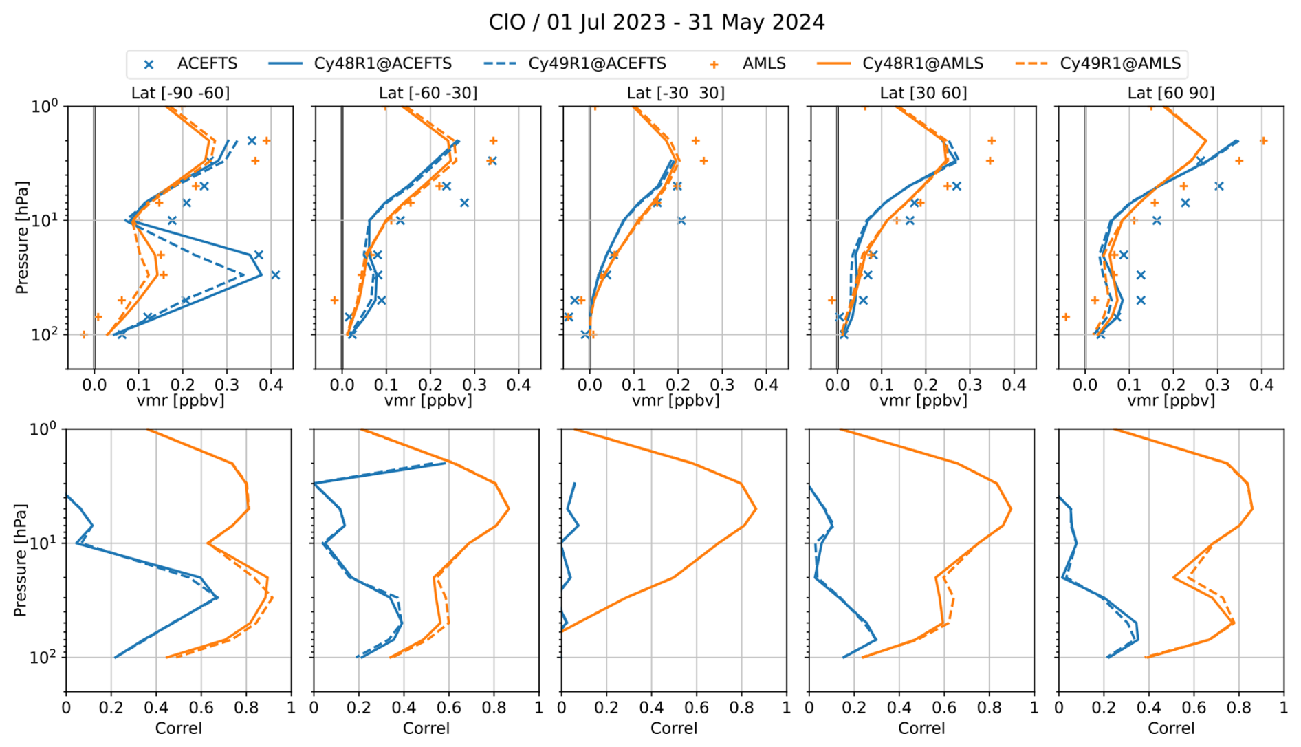
Figure 7 Same as Fig. 4 but for ClO and showing only the volume mixing ratios and correlations. The number of profiles used in each comparison are nearly identical with those used for HCl (see previous Figure).

Considering these difficulties, the evaluation of ClO provides some satisfactory agreement with respect to the general features of the distribution (Fig. 7, top row). The shapes of the vertical profiles are well captured, including the maxima at the correct level in the polar lower stratosphere. This signature of chlorine activation is evaluated in more detail and with tailored experiments in Sect. 6.

5.5  NO_x

NO₂ is a primary global product for CAMS, primarily for the monitoring of air quality in the lower troposphere. High-resolution tropospheric columns of NO₂ can be retrieved from nadir-looking instruments such as TROPOMI but this requires a good knowledge of the stratospheric column (van Geffen et al., 2022). ACE-FTS data are available to evaluate vertical profiles of stratospheric NO₂ but the interpolation of three-hourly output from IFS-COMPO may lead to undesirable errors, as was shown for ClO. We choose to evaluate instead the NO_x family (defined as the sum of NO and NO₂), which has a longer lifetime and is thus easier to compare with observations from a solar occultation instrument such as ACE-FTS. For the evaluation of NO_x (Fig. 8), we display its partial pressures rather than its volume mixing ratio in order to highlight differences in the lower stratosphere which contribute most to the stratospheric column.

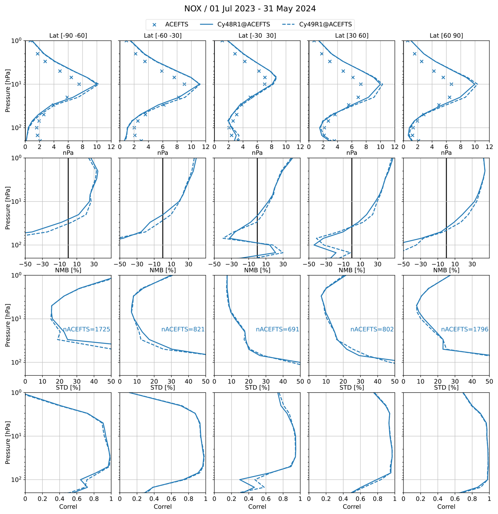
Figure 8 Same as Fig. 4 but for NO_x (i.e. NO+NO₂), using only ACE-FTS observations, and with the top row showing partial pressures in nPa.

Figure 8 shows differences increasing continuously with altitude, with a severe model underestimation in the lower stratosphere (approximately −30 % at the 50 hPa pressure level in all latitude bands), and a severe model overestimation in the upper stratosphere (30 % to 40 % at the 2 hPa pressure level). The standard deviation exceeds 20 % below (i.e. at pressures higher than) 40 hPa while the correlations with values larger than 0.8 are obtained in most stratospheric regions. The upgrade of IFS-COMPO to Cy49R1 shows a slight improvement in the lower stratosphere, especially with respect to the standard deviations and the correlations in the Southern Hemisphere (SH) and in the Tropics. The underestimation of NO₂ in the lower stratosphere correlates well with HNO₃ underestimation, suggesting again deficiencies in the modelling of heterogeneous chemistry and the partitioning between gaseous and condensed phases.

The overestimation of NO_x in the upper stratosphere is due to a large overestimation of nighttime NO₂. This is a recurrent feature of the BASCOE stratospheric chemistry module, as shown already by the control run for an early analysis of MIPAS NO₂ (Errera et al., 2008), and its implementation in the Canadian NWP model GEM (Fig. S8 in Ménard et al., 2020) and in the evaluation of the first implementation of BASCOE in IFS-COMPO (Huijnen et al., 2016). The IFS-COMPO Cy49R1 experiments which were set up to evaluate polar ozone depletion during earlier years, using temperature and winds from ERA5 (see Sect. 4.2), deliver similarly biased NO₂ in the upper stratosphere (not shown). The early IFS-COMPO experiments (Huijnen et al., 2016) used ERA-Interim temperatures, which were less biased than ERA5 temperatures with respect to independent observations in the upper stratosphere (Simmons et al., 2020; Marlton et al., 2021). The persistence of these biases with different meteorological (re-)analyses indicate that they are probably not due to temperature biases in the upper stratosphere. They are not related either to the photolysis rate of NO₂ as this rate is computed by completely different algorithms in the BASCOE CTM and in IFS-COMPO (see Sect. 2.1). Nor can they be due to differences in the nitrogen source, because the N₂O biases in Huijnen et al. (2016) and in this work (see Sect. 5.1) have opposite signs while the upper stratospheric NO₂ bias remains positive – and unexplained.

5.6  O₃

O₃ analyses and forecasts are the most important stratospheric products of CAMS, with a focus on the lower stratosphere (pressures larger than 10 hPa) which contributes most to the total ozone column. As for NO_x, the evaluation of O₃ (Fig. 9) displays partial pressures rather than its volume mixing ratio in order to highlight differences in this layer. Both ACE-FTS (Sheese et al., 2022) and Aura-MLS (Livesey et al., 2022) ozone retrievals have a reported accuracy smaller than 10 % in the whole vertical range of the evaluation, i.e. in the 1–200 hPa pressure range. In the lower stratosphere (20–150 hPa pressure range), the biases with IFS-COMPO Cy49R1 vary between −10 % and 10 % in all latitude bands and are thus very comparable to these observational accuracies. This is a significant improvement with respect to the Cy48R1, which underestimated ozone by 30 % to 50 % in the lowermost levels of the extratropical stratosphere. The standard deviation also improves in the lowermost stratosphere and in the polar lower stratosphere with the model upgrade, decreasing at 150 hPa from 25 %–30 % to 20 %–25 % in all latitude bands, at 20 hPa from 12 % to 7 % in the 90–60° S latitude range, and at 50 hPa from 8 %–5 % to 5 %–4 % in the 60–90° N latitude range. The standard deviation reaches values as low as 5 % in the middle stratosphere (i.e. in the 5–20 hPa pressure range) with both cycles of IFS-COMPO, and the correlations between models and observations are larger than 0.8 in all latitude bands and pressure levels, except for a few levels in the tropical and South Pole lowermost stratosphere. Overall, the model evaluation is very satisfactory in the lower stratosphere, especially considering the absence of any assimilation of composition data, and highlights improvements between the two latest cycles of IFS-COMPO.

Figure 9 Same as Fig. 4 but for O₃ with the top row showing partial pressures in mPa.

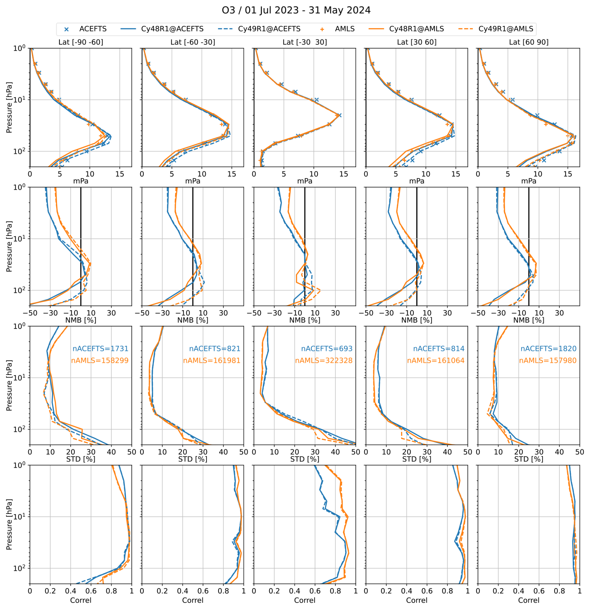
This contrasts with the IFS-COMPO biases in the upper stratosphere, where ozone is negatively biased by 2 % to 25 % in the Tropics and mid-latitudes, and by 10 % to 35 % in the polar regions. This is beyond the reported observational accuracy at most levels with pressure smaller than 10 hPa. In all latitude bands this upper stratospheric ozone deficit is more pronounced against ACE-FTS than against Aura-MLS and increases with decreasing pressures. It is accompanied by slight increases of the standard deviation, which remain nonetheless well below 10 % at extrapolar latitudes and 15 % in the polar regions.

Let us provide some context with earlier cycles of IFS-COMPO and the recent history of its operational production, which includes assimilation of Aura-MLS ozone retrievals. Stratospheric ozone in IFS-COMPO Cy47R1, which became operational in October 2020, was much improved by the introduction of the Hybrid Linear Ozone (HLO) scheme, a Cariolle-type linear parameterization of stratospheric ozone chemistry using as mean state a climatology derived from observations (Eskes et al., 2020). Eskes et al. (2024a) evaluated the operational analyses and five-day forecasts of ozone by IFS-COMPO Cy47R3 and Cy48R1 (respectively named “o-suite” and “e-suite” at that time) and reported a larger negative bias in the upper stratosphere with Cy48R1 than with Cy47R3. The ozone deficit found in the upper stratosphere with the BASCOE module is not entirely corrected by the assimilation of ozone retrievals from Aura-MLS. This increased ozone deficit is the only degradation in the stratospheric composition observed in the upgrade of Cy47R3 to Cy48R1, and it is still not corrected by the next upgrade to Cy49R1 (Eskes et al., 2024b).

The BASCOE CTM also underestimates MLS ozone by ∼20 % around 1 hPa (Skachko et al., 2016). Exactly in the same way as for the NO₂ overestimation, an ozone deficit in the upper stratosphere has been consistently obtained with all models containing the BASCOE stratospheric chemistry module, independently of their input meteorological analyses, transport algorithms, and initialization details (Errera et al., 2008; Huijnen et al., 2016; Ménard et al., 2020). The first implementation of BASCOE in IFS-COMPO evaluated an alternative set-up where tropospheric chemistry and stratospheric chemistry modules were merged by using a single reaction mechanism and the same solver in both regions. This integrated set-up yielded essentially the same ozone deficit in the upper stratosphere than the set-up with separate tropospheric and stratospheric chemistry modules that was kept for further developments (Huijnen et al., 2016).

The NO₂ overestimation and ozone deficit in the upper stratosphere are probably due to the same cause, but the issue remains unsolved and requires further research. Diouf et al. (2024) reported a similar ozone deficit in the upper stratosphere–lower mesosphere with the REPROBUS CTM and proposed a dual explanation: an overestimation of the temperatures in the meteorological analyses, and a missing source of ozone from highly vibrationally excited states of molecular oxygen.

5.7 Aerosol extinction coefficients

Figure 10 compares the simulated and retrieved extinction profiles at three different wavelengths (see legend) for nearly a year of simulation spanning 2023 and 2024. No volcanic injection is simulated for the operational analyses and short-term forecasts, as they rely only on data assimilation to represent the volcanic signal. We evaluate here the corresponding control runs, which do not assimilate any aerosol-related data. The two IFS-COMPO simulations evaluated here contain thus only the quiescent component of the stratospheric aerosol loading.

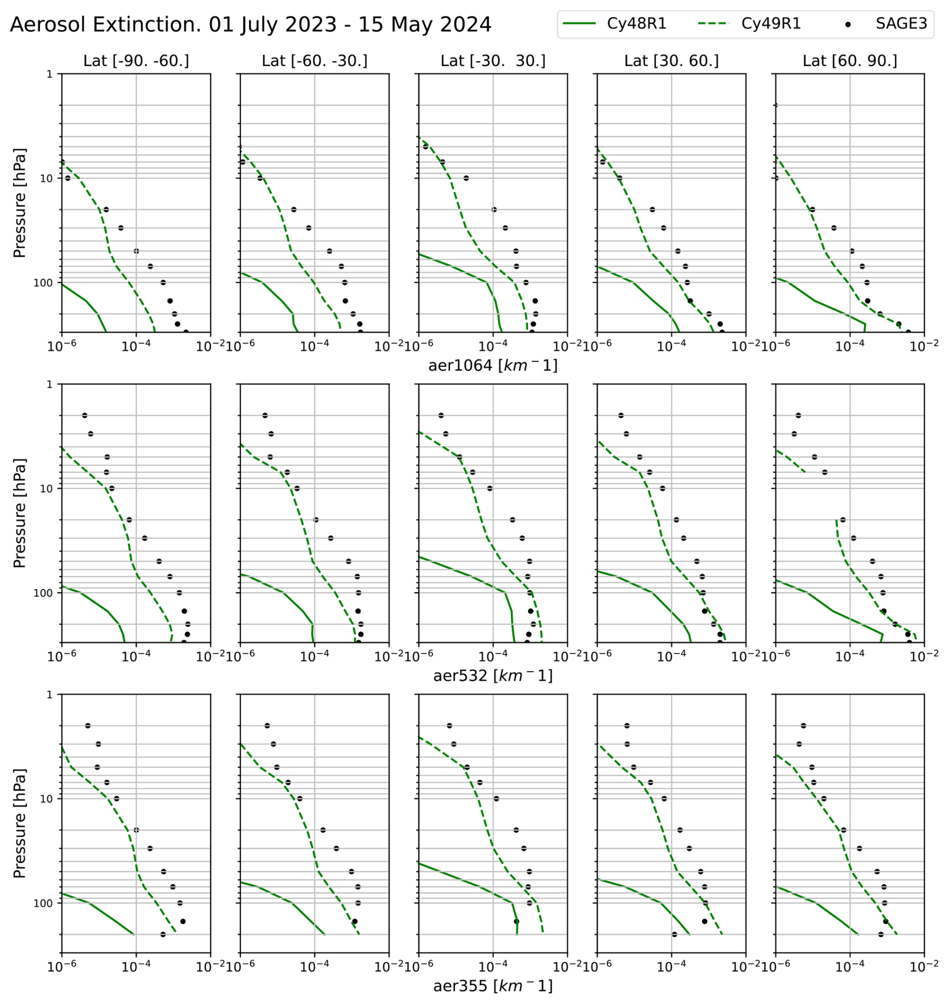
Figure 10 Comparison of mean aerosol extinction coefficients profiles at three different wavelengths over the same five latitude bands as in Fig. 5, for the period between 1 July 2023 and 31 May 2024: SAGE III/ISS observations (black dots) versus control runs of IFS-COMPO Cy48R1 (solid lines) and Cy49R1 (dashed lines). The IFS-COMPO aerosol extinction coefficients are compared at wavelengths 1064 (top row), 532 (middle row) and 355 nm (bottom row) with the closest wavelengths observed by SAGE III/ISS (respectively 1021, 521 and 384 nm).

The very large underestimation of Cy48R1 was caused by the lack of production of stratospheric sulfate. The implementation of new processes leading to the production of stratospheric sulfate in Cy49R1 increased significantly the simulated stratospheric aerosol extinction at all three wavelengths and brings a significant improvement at all levels, for all regions and for the three considered wavelengths. The vertical profiles of simulated extinctions match relatively well the retrievals, especially the constant or slow increase of retrieved extinction with pressure from ∼5 to ∼30 hPa and the stronger increase from ∼30 to ∼150 hPa. The low bias remaining in the middle stratosphere is due, at least in part, to the lack of any volcanic injection. The signal of the Hunga eruption, for example, is not represented and addressed in another study (Zhu et al., 2025).

6 Evaluation of seven polar winter-spring seasons between 2008 and 2020

6.1 H₂O and HNO₃

Figure 11 shows that IFS-COMPO Cy49R1 simulates a realistic distribution of water vapour in the lower Arctic stratosphere, compared against BRAM3, with the normalized biases never exceeding 3 %. The seasonal evolution of water vapour in the Antarctic polar vortex is somewhat more difficult to capture. The BRAM3 reanalysis shows very consistent behaviour across all four simulation years, with constant values until mid-June when condensation starts abruptly. This starts two weeks earlier in IFS-COMPO and develops at a slower rate, leading to an underestimation of H₂O of 5 % which remains approximately constant until the end of polar winter in September 2008 and September 2009. The 2020 Antarctic winter-spring season shows a different behaviour, with a surge of water vapour in the reanalysis starting in mid-July and lasting two weeks. The model fails to capture this event, leading to an additional bias of nearly −10 % compared with the two other considered years (2008 and 2009). Hence the underestimation of water vapour reaches −15 % in August 2020 and lasts three more months than in 2008 and 2009. Overall, Fig. 11 shows quite satisfactory results, especially considering the very simple approach adopted for the dehydration, which is considered here to be solely due to sedimentation of ice PSC particles (Huijnen et al., 2016). Even though the corresponding biases are difficult to disentangle from those introduced by downward transport in the vortex and horizontal transport across the vortex edge, we found here that they always remain in the range −20 % to 5 % for the seven events shown, which are influenced by very different meteorological conditions. Similar results are obtained for N₂O before 2013 (Fig. S6 in the Supplement).

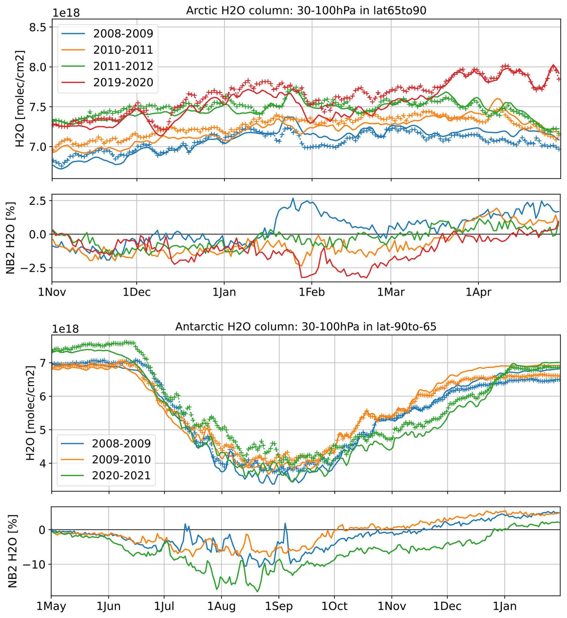
Figure 11 A time series of the H₂O partial columns (30–100 hPa, upper panels) in IFS-COMPO Cy49R1 chemical forecasts (solid lines) and in the BRAM3 reanalysis (crosses), and the corresponding normalized biases (lower panels). Comparisons are shown for both the Arctic (65–90° N, top) and the Antarctic (90–65° S, bottom) for the same years and using the same color scheme as in Fig. 3.

The time series of HNO₃ in polar winter and spring (Fig. 12) exhibit larger biases than those for H₂O (Fig. 11) with respect to the corresponding BRAM3 reanalyses. While these biases mostly remain in the range ±5 % in the Arctic during the typical winter-spring seasons 2008–2009 and 2011–2012, larger biases are observed during years with exceptional meteorological conditions (i.e. 2010–2011 and 2019–2020), reaching ±10 % during December and January. Furthermore, the impact on HNO₃ of the 2020 springtime vortex is less adequately captured by the model than the similar episode in 2011. According to BRAM3, the decrease in HNO₃ slowed down in February after the steep decrease during the end of January 2020. On the contrary, HNO₃ simulated in IFS-COMPO keeps decreasing, developing an underestimation of 10 % which worsens further to nearly 20 % in March and barely starts recovering during April 2020.

Figure 12 Same as Fig. 11 but for HNO₃.

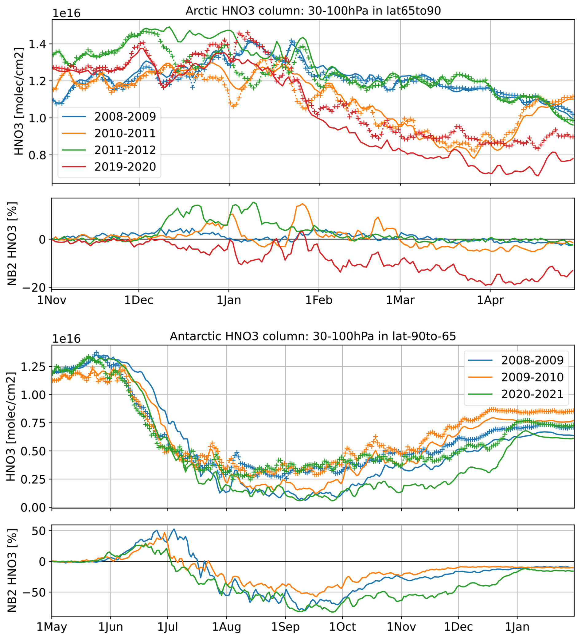
The depletion of HNO₃ above the Antarctic (bottom of Fig. 12), which is related to the presence and abundance of NAT PSC, starts one or two weeks later in IFS-COMPO than in the BRAM3 reanalysis. It proceeds more quickly and lasts until mid-September, while the HNO₃ recovery already starts at the beginning of August according to the BRAM3 reanalysis. A pattern of too intense HNO₃ depletion is thus obtained for polar vortex conditions. The resulting significant underestimation of HNO₃ during austral winter (up to 75 % in mid-September) is strongly highlighted by the bias normalization: the corresponding absolute biases (not shown) are not larger than those obtained in June. We attribute this disagreement to the overly simple PSC parameterization in the model which does not account for gravitational settling (see Sect. 2.2). Reinforcing our interpretation, the HNO₃ evolution during the year 2020 shows a similar behaviour: due to the fact that the vortex was exceptionally long-lasting and dissipated only in mid-December, the corresponding HNO₃ underestimation recovers two months later than in either 2008 or 2009.

6.2 HCl

Seasonal changes and interannual variability of HCl are a key indicator of the polar chemistry enabled by heterogeneous reactions on the surface of PSC particles (Solomon et al., 2015) but remain difficult to capture with state-of-the-art models (Grooß et al., 2018). The positive biases of the HCl timeseries (Fig. 13) are not consistent with the negative biases found in the polar lower stratosphere in the two control runs (Fig. 6). Rather than being an effect of interannual variability, we attribute this disagreement to the different initializations of HCl: the control runs discussed in the previous section had not been constrained by any observations of composition during the earlier runs, while the experiments discussed in this section are initialized from BRAM3 at the beginning of winter (see Sect. 4.2). This highlights the importance of the initial conditions for chemical forecasts in the stratosphere.

Figure 13 Same as Fig. 11 but for HCl.

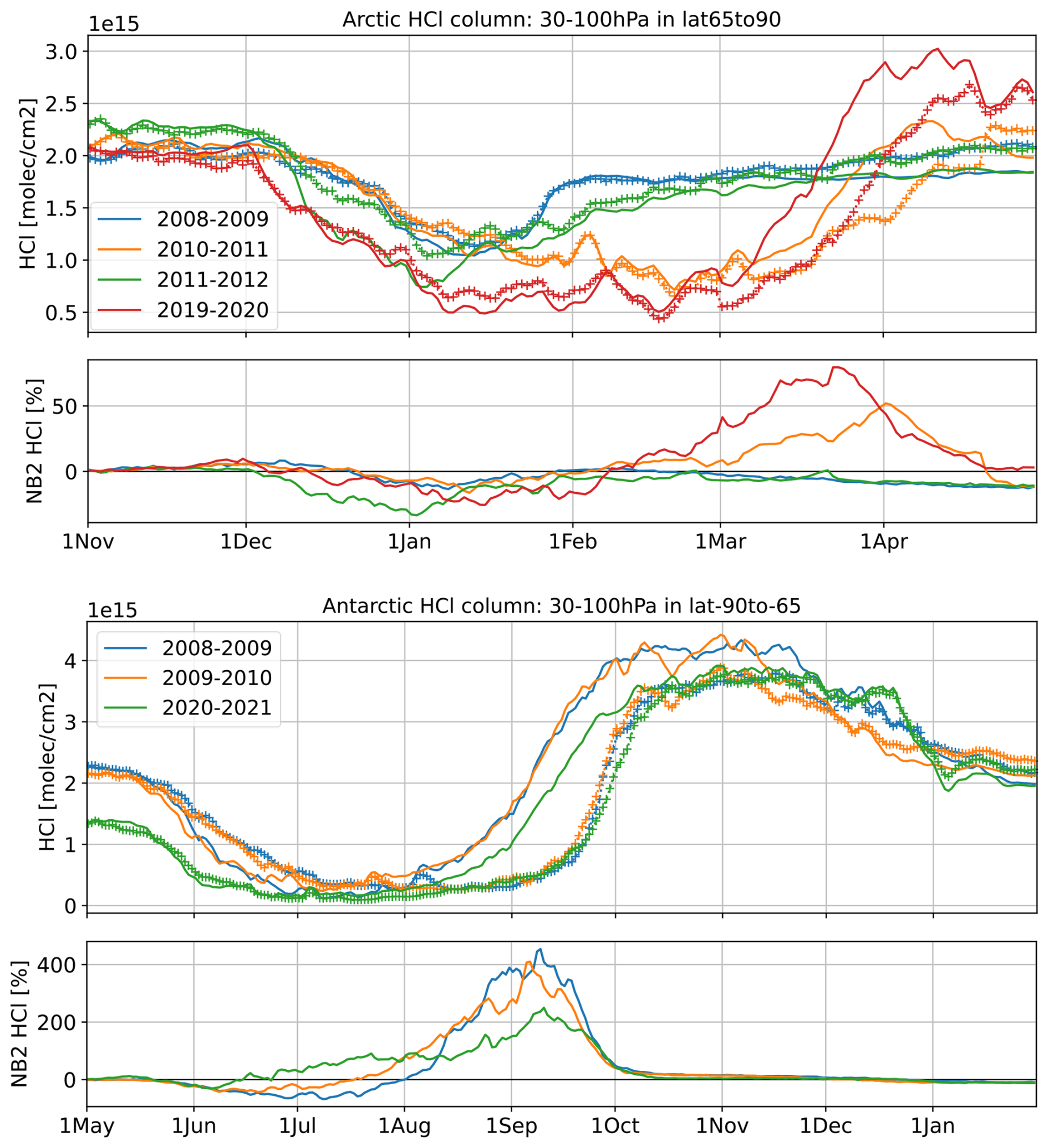
Figure 13 shows that the HCl partial columns simulated by IFS-COMPO are captured well at the beginning and the end of each winter-spring season but also highlight difficulties in modelling correctly the initial rate of this depletion, as well as its duration. HCl depletion is too fast at the beginning of winter-spring seasons for some years, i.e. over the Arctic in December 2011 and over the Antarctic in June 2008 and June 2009. The mid-season recovery of HCl presents different issues over the Arctic and over the Antarctic. Over the Arctic, this recovery starts at the correct date (i.e. in January for years 2008 and 2009, and in March for years 2011 and 2020) but takes place too rapidly during the two seasons with unusual O₃ depletion (March 2011 and 2020).

Above the Antarctic, the period of HCl depletion is too short, with recovery starting as early as July or August, whereas in the Aura-MLS reanalyses it starts systematically in September with the return of light (see also the ClO timeseries below). Furthermore, the rate of recovery above the Antarctic is remarkably independent of the simulated year and is generally too slow in IFS-COMPO compared to the reanalyses. As a result, positive HCl biases develop in the middle of every O₃ hole event (i.e. 2011 and 2020 above the Arctic and every year above the Antarctic), reaching very large values: approximately 50 % and 80 % in late March 2011 and 2020, respectively; 400 % in September 2009; and 200 % in September 2020. These HCl biases (Fig. 13) are much larger than those simulated for either H₂O (Fig. 11) or HNO₃ (Fig. 12) and the impact of meteorology is much more pronounced, i.e., the biases for the Arctic 2011 and 2020 and in the Antarctic 2020 are significantly higher when compared with the other years.

Remarkably, the exceptional meteorological conditions which occurred in the Antarctic 2020 event do not give rise to any detectable signature for HCl in the Aura-MLS reanalyses: as shown in Fig. 13, the observed recovery starts at exactly the same date and rate in 2020 as in both 2008 and 2009. This insensitivity to the specific dynamics of the Antarctic winter confirms that HCl will be a prime target for improvement if the PSC parameterization of the BASCOE module is replaced by a more sophisticated modelling approach in the future.

Previous CTM studies of polar O₃ depletion have also reported on HCl biases. As an example, Grooß et al. (2018) discussed the model overestimation of HCl at the beginning of the season by the stratospheric models CLaMS, SD-WACCM and TOMCAT/SLIMCAT. While they speculated about the existence of an unknown process in such state-of-the art models to explain such biases, the early-season biases reported by Grooß et al. (2018) are positive while in IFS(CBA) they are negative. We cannot investigate such aspects with the oversimplified parameterization of PSC in the BASCOE module currently employed in IFS-COMPO Cy49R1.

6.3 ClO

In the springtime polar stratosphere, catalytic destruction of stratospheric O₃ by chlorine compounds is induced by active chlorine in the form of the family ClO_x, with very rapid cycling between its three members Cl, ClO and Cl₂O₂. The availability of Aura-MLS observations of ClO (Nedoluha et al., 2016) allows us to easily evaluate the amount of PSC-activated chlorine in IFS-COMPO through the corresponding reanalysis in BRAM3. Figure 14 shows that, above the Arctic, chlorine activation happens not only in spring after winters with an exceptionally stable vortex (i.e. February–March 2011 and 2020) but also starts every year in December, as first reported from aircraft-borne measurements during the SOLVE/THESEO-2000 campaign (Bremer et al., 2002; Stimpfle et al., 2004). This activation lasted until the end of January in the 2009 case, and mid-February in the 2012 case (partial columns reaching 2–$\mathrm{4}\times {\mathrm{10}}^{\mathrm{14}}{\mathrm{cm}}^{-\mathrm{2}}$). For the exceptional years of 2011 and 2020, ClO kept increasing until mid-March (resulting in columns as large as 4–$\mathrm{5}\times {\mathrm{10}}^{\mathrm{14}}{\mathrm{cm}}^{-\mathrm{2}}$), after which mixing ratios became very small due to the breakup of the vortex. It is encouraging to see that the timing and intensity of ClO abundance is captured accurately by IFS-COMPO Cy49R1; there is a tendency to overestimate the wintertime partial columns by around 15 %–25 % but seasonal and interannual variations remain very well captured, especially considering the exceptional episodes of March–April 2011 and 2020.

Figure 14 Same as Fig. 11 but for ClO and showing absolute rather than normalized biases.

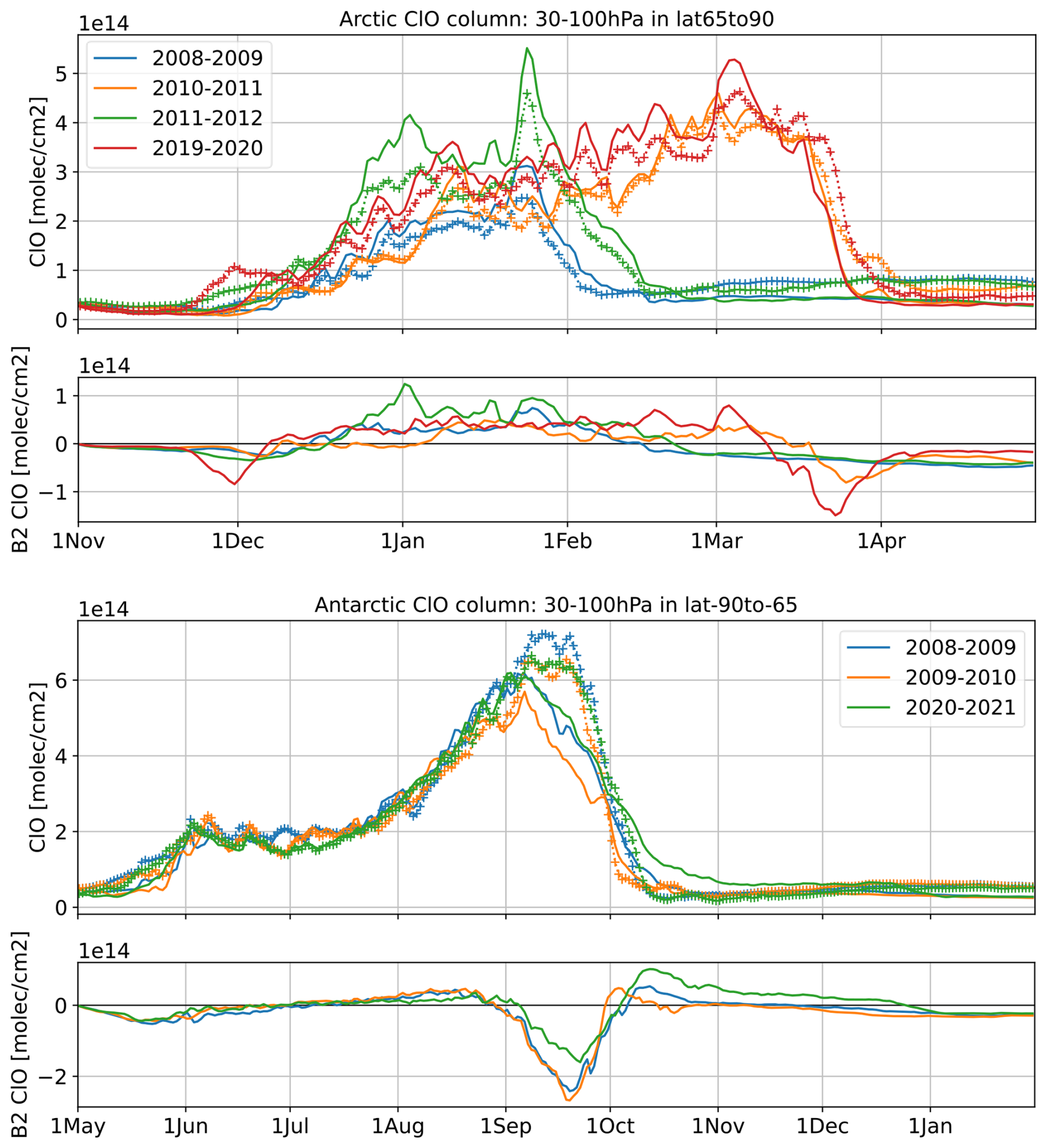
Over the Antarctic, the reanalyses indicate remarkably little interannual variability with partial columns consistently increasing to $\mathrm{2}\times {\mathrm{10}}^{\mathrm{14}}{\mathrm{cm}}^{-\mathrm{2}}$ in wintertime, increasing from mid-July until the end of August to reach 6–$\mathrm{7}\times {\mathrm{10}}^{\mathrm{14}}{\mathrm{cm}}^{-\mathrm{2}}$ in mid-September, before quickly decreasing back to near-zero values during the first week of September. Although IFS-COMPO agrees remarkably well with the BRAM3 reanalysis during austral winter, we observe a sudden drop early September, i.e. two weeks too early, leading to a significant underestimation until the end of that month. This is correlated with the September warm-up in the 30–100 hPa layer (see Fig. 3) and we interpret it as a consequence of the premature HCl recovery in IFS-COMPO during the same month (see Fig. 13). In September 2020, the bias was reduced by approximately 50 % compared to the same month in 2008 and 2009 and showed afterwards an unexpectedly slow decrease during the whole month of October 2020. This unusual behaviour may be associated with unusual transport in August–September of that year (see H₂O, Fig. 11) and obviously with the less severe HCl bias in September 2020 than in September 2008–2009 (see Fig. 13).

Overall, active chlorine is remarkably well modelled in the Arctic and in the wintertime Antarctic, but the model fails to capture the high concentrations in September of the reanalyses, due to the early recovery of the HCl reservoir. This confirms the importance of improving HNO₃ and HCl through an improvement of the PSC parameterization in future developments of IFS-COMPO.

6.4  NO₂

Figure 15 compares NO₂ with a BASCOE reanalysis of MIPAS by the updated 4D-VAR BASCOE DAS (see Sect. 3.3). The nighttime destruction of NO₂ during wintertime (Marchand et al., 2003) is well captured by IFS-COMPO. At the end of the winter and beginning of the spring, the rate of NO₂ increases following a timing that is also well captured by the model. The springtime NO₂ columns are systematically underestimated compared to the reanalysis of MIPAS, which is consistent with the global comparison of NO_x between the control runs and ACE-FTS measurements (see Sect. 5.5).

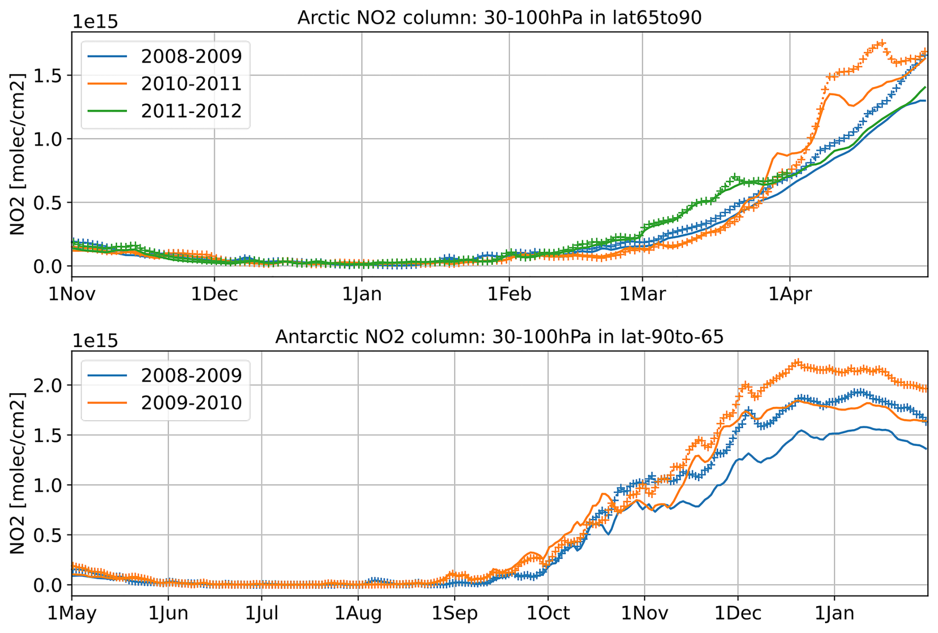
Figure 15 Comparisons of time series of the NO₂ partial columns (30–100 hPa) from IFS-COMPO Cy49R1 chemical forecasts (solid lines) and from the BASCOE reanalysis of MIPAS (crosses) in the Arctic (65–90° N, top) and in the Antarctic (90–65° S, bottom), for the winter-spring seasons of 2008–2009 (blue), 2010–2011 (orange) and 2011–2012 (green, Arctic only).

6.5 BrO and BrONO₂

Bromine atoms can either destroy O₃ directly or recombine with atomic chlorine to form BrCl, thereby decreasing the amount of active chlorine and slowing down O₃ destruction. Here we use the UV-Vis spectrometer at Harestua (see Sect. 3.2) to perform a first evaluation of BrO in the Arctic region.

Figure 16 shows that the order of magnitude of BrO stratospheric columns in IFS-COMPO is correct, with an excellent agreement during the beginning of winter followed by slight overestimation which lasts longer in 2008–2009 (December to March) than in 2019–2020 (March only). Using the BASCOE CTM to simulate the 2008–2009 season with chemical rates updated to JPL evaluation 19 (Burkholder et al., 2020), we assess that this overestimation is due to outdated chemical rates for the destruction of CHBr₃ and CH₂Br₂ in IFS-COMPO Cy49R1.

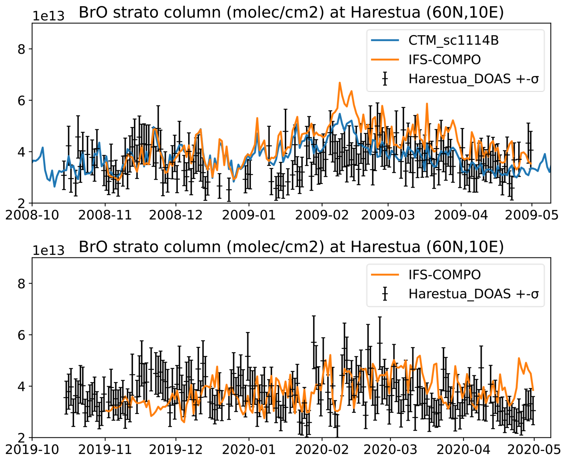
Figure 16 A time series of the stratospheric BrO Vertical Column Density above Harestua (60.2° N, 10.8° E) during the 2008–2009 (top) and 2019–2020 (bottom) winter-spring seasons. Black symbols and error bars: UV-Vis DOAS retrievals adjusted to 13:30 LT with a box-model; solid lines: results by IFS-COMPO Cy49R1 (orange) and by the BASCOE CTM with an updated chemical scheme (blue, 2008–2009 only) at noon UT.

Figure S7 in the Supplement shows the evolution of the BrO radical simulated in IFS-COMPO Cy49R1 at 100 hPa in the Arctic for both 2008–2009 and 2019–2020. During typical years such as 2008–2009, maximum values are reached above the North Pole at the end of spring, while the exceptional polar chemistry of springtime 2020 results in a noticeable drop in number density in BrO at the end of March and the beginning of April, i.e. just after heterogeneous chemistry has ended (see ClO, Fig. 16). Unfortunately this decrease does not extend equatorward of 70° N and this signal does not reach the Harestua station – neither in the observations nor in the model.

Bromine nitrate (BrONO₂) is the most important nighttime reservoir of bromine (Höpfner et al., 2021). It is produced by the reaction between BrO and NO₂ and is destroyed during daytime by photolysis producing Br and BrO (Burkholder et al., 2020). BrONO₂ concentration shows strong day/night variations with maximum values reaching 25 pptv at night (Höpfner et al., 2009). Since the signal is much larger during the night, we show only nighttime values of BrONO₂ concentration for both MIPAS and IFS-COMPO output.

Figure 17 shows a time series of nighttime BrONO₂ concentration at 50 hPa during the winter-spring season over several years for the Arctic and the Antarctic. We find a good agreement above the Arctic with low BrONO₂ concentration during winter due to conversion of BRONO₂ from heterogeneous reactions on the PSC particles (Höpfner et al., 2021). During austral winter-spring, IFS-COMPO finds low BrONO₂ concentration values compared to MIPAS, which is consistent with the control run underestimation of NO_x at 50 hPa over the Antarctic with respect toACE-FTS (see Sect. 5.5). While the MIPAS dataset of BrONO₂ shows a gradual recovery very early in austral winter, this recovery is delayed by about two months in IFS-COMPO and occurs much more quickly in September.

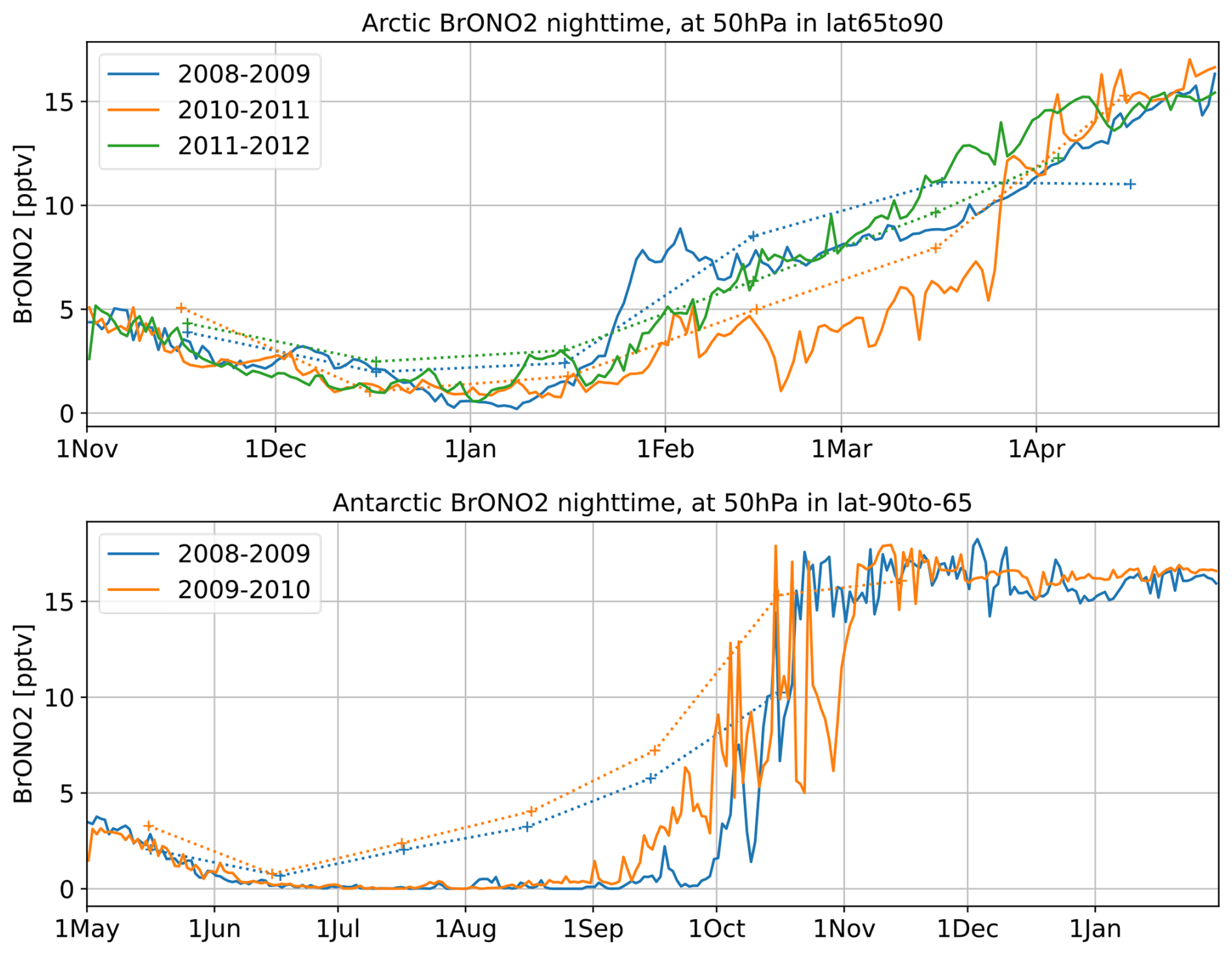
Figure 17 Same as Fig. 15 but for nighttime (i.e., solar zenith angle >90) BrONO₂ volume mixing ratios at the 50 hPa pressure level, using MIPAS monthly means as references (dotted lines; Höpfner et al., 2021).

6.6  O₃

Figure 18 shows that negative biases in stratospheric O₃ in IFS-COMPO appear only in very stable polar vortex conditions, with quite different behaviours in the Arctic for the years 2011 and 2020 compared to the Antarctic. For the Arctic “Ozone hole” episodes of 2011 and 2020, the modelled O₃ decreases more quickly than in the reanalysis, and remains biased low until the end of the episode, with a maximum underestimation at the time of the O₃ minimum i.e. in March 2011 (12 DU) and March 2020 (18DU).

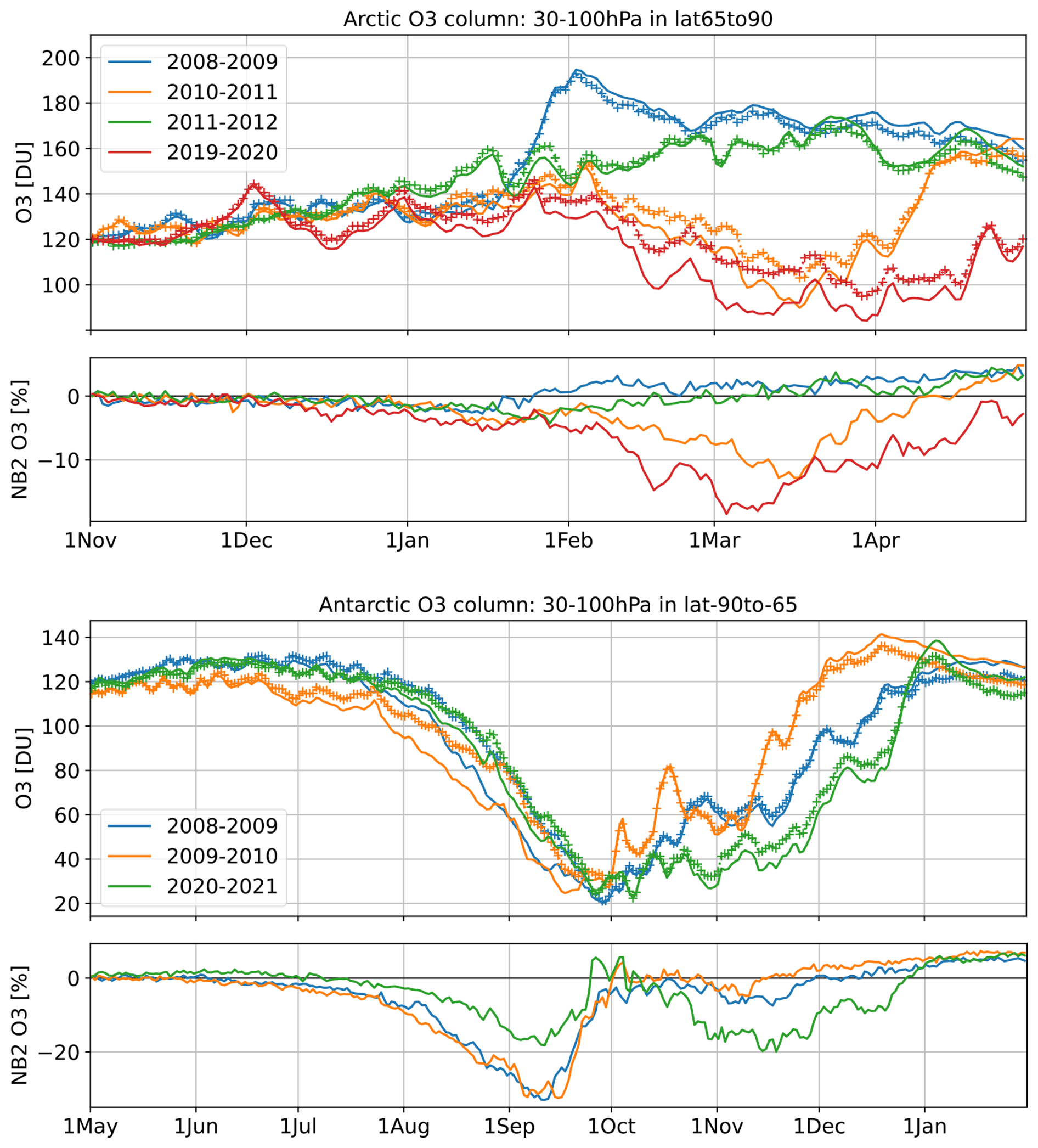
Figure 18 A time series of the O₃ partial columns in Dobson units (30–100 hPa, upper panels) in IFS-COMPO Cy49R1 chemical forecasts (solid lines) using the BRAM3 reanalysis as a reference (crosses), and the corresponding biases (lower panels). Comparisons are shown for both the Arctic (65–90° N, top) and the Antarctic (90–65° S, bottom) for the same years and using the same color scheme as in Fig. 3.

In the Antarctic, the wintertime behaviour is similar, but the O₃ underestimation disappears very rapidly when O₃ depletion reaches its maximum (end of September-beginning of October) i.e., when many processes involving PSCs reach their saturation point (Tritscher et al., 2021, Sect. 6.2). This explains that despite the underestimation of ClO observed in September, no bias remains by early October in any of the three Antarctic O₃ hole experiments. The Antarctic 2020 episode stands out again: during August the low bias is twice smaller than in the same month of 2008 and 2009, and in October–November the model captures successfully the exceptional duration of the O₃ hole – which was not necessarily expected. Yet, a low bias appears again and lasts until the end of the season, quite similar to the results obtained in the Arctic spring of 2011 and 2020.

To conclude, IFS-COMPO shows overall good performance but with a tendency to overestimate O₃ depletion during exceptionally long cold seasons in the Arctic and at the beginning of the season in the Antarctic. During the exceptional Antarctic O₃ hole in 2020, O₃ biases are unusually large but not larger than in 2008 or 2009. It is not possible to identify the causes of these O₃ biases by looking at O₃ only, but the large HCl biases point to shortcomings in the PSC parameterization.

7 Summary scorecard of gas-phase chemical forecasts in the stratosphere of IFS-COMPO Cy49R1

In view of the range of stratospheric gas-phase species evaluated in the two previous sections, and the diversity of the evaluation results across the different layers and latitudinal regions of the stratosphere, we choose to summarize the results of this evaluation in a synthetic scorecard (Fig. 19). This approach is similar to that presented in the comprehensive evaluation of Cy48R1 by Eskes et al. (2024a) but provides an assessment on the absolute performance of Cy49R1 rather than the relative improvement from Cy48R1 to Cy49R1.

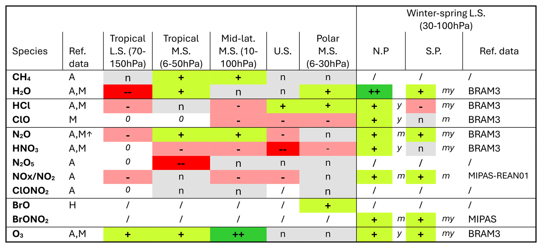
Figure 19 Scorecard for the performance of chemical forecasts in the stratosphere of IFS-COMPO Cy49R1 against observations and chemical reanalyses for 13 gas-phase species in five regions of the global stratosphere and for the winter-spring polar lower stratosphere. The five regions of the stratosphere are defined by latitudes and pressures as follows: tropical lower stratosphere (L.S.): 30° S–30° N, 70–150 hPa; tropical middle stratosphere (M.S.): 30° S–30° N, 6–50 hPa; mid-latitudes M.S.: 60–30° S and 30–60° N, 10–100 hPa; upper stratosphere (U.S.): 2–6 hPa in the Tropics, 2–10 hPa in the extra-Tropics; polar M.S.: 90–60° S and 60–90° N, 6–30 hPa. The winter-spring polar L.S. distinguishes the South Pole (S.P., 90–65° S) and the North Pole (N.P., 65–90° N). The performance is evaluated as “$++$” (very good), “+” (good), “n” (neutral i.e. acceptable), “-” (poor) or “–” (very poor). “0” indicates that the observed vmr is too small to allow evaluation. For the five regions of the global stratosphere this assessment relies on objective criteria derived from Sect. 5, and for the winter-spring polar L.S. it summarizes Sect. 6 (see text for details and reference datasets).

Figure 19 summarizes the performance of IFS-COMPO Cy49R1 with respect to stratospheric gas-phase species in the absence of chemical data assimilation. It is split into a left-side part which synthesizes the global statistical diagnostics of the e-suite control run (see Sect. 5), and a right-side part which summarizes the evaluation in the polar lower stratosphere during several winter-spring seasons (see Sect. 6). The order of regions follows broadly the Brewer–Dobson Circulation (BDC), from its entry point in the tropical lower stratosphere through is ascent in the tropical middle stratosphere, transport into the mid-latitudes mid-stratosphere, and descent into the polar stratosphere. The extratropical lower stratosphere (pressures larger than 100 hPa) is out of scope for this paper.

The regional scores are determined objectively from the absolute values of the Normalized Mean Bias (NMB), Standard Deviations of differences between model and observations (STD) and corresponding correlations, using criteria chosen to segregate between the four proposed scores while prioritizing bias performance (see Table S1 in the Supplement). These scores are computed separately for each reference dataset (second column: “A” for ACE-FTS; “M” for Aura-MLS) and added for the species where both datasets are available. The total score provides a combined performance assessment, requiring the availability and agreement with both ACE-FTS and Aura-MLS to allow “very good performance” assessment (see Table S2 in the Supplement for details). This approach implies that if the two reference datasets do not agree, the model will inevitably receive a lower score. The assessment for N₂O in the lower and middle stratosphere relied only on ACE-FTS because Aura-MLS shows suspiciously large disagreements at pressures larger than 10 hPa while difficulties were reported in the retrieval of Aura-MLS N₂O v4 (see Sect. 3.3).

The polar lower stratospheric scores summarize in a more subjective manner the ability of the model to capture the timing and rate of changes during winter-spring seasons, i.e. the intraseasonal variability on timescales from weeks to months, as well as the interannual variability, as evaluated in Sect. 6 with two reanalyses of stratospheric composition (see last column and Sect. 3.3 for details). Some polar L.S. scores are labelled with a combination of letters m, y to note difficulties capturing intraseasonal variability (monthly timescales) and/or interannual variability (yearly timescales).

The 12 gas-phase species included in Fig. 19 are grouped into families, namely: hydrogen source (CH₄) and reservoirs (H₂O), chlorine reservoir (HCl) and reactive radical (ClO), nitrogen source (N₂O) and reactive gases (HNO₃, N₂O₅, NO_x, ClONO₂), bromine reservoir (BrONO₂) and radical (BrO) and, finally, O₃ which is the primary stratospheric target of CAMS. The score for BrO is based on the bias of the stratospheric column in winter-spring 2008–2009 and 2019–2020 with respect to the UV-Vis spectrometer at Harestua (“H” in the second column; see Sect. 6.4).

Figure 19 highlights the successes as well as areas for further research and development in the stratosphere of IFS-COMPO Cy49R1, e.g. with respect to the nitrogen reactive species. These points have been discussed in the two previous sections and will be summarized in the Conclusions.

8 Evaluation of the stratospheric aerosols resulting from the Pinatubo eruption

Figure 20 shows a comparison of stratospheric sulfate burden simulated by IFS-COMPO against that retrieved from experimental measurements after the Pinatubo eruption. The rapid increase of the sulfate burden is well represented by IFS-COMPO with the peak of stratospheric sulfate burden being timed correctly. However, a positive bias of nearly 20 % is found when compared to both HIRS and SAGE-3λ products, equating to around 1 TgS overestimation in the stratospheric mass. The rate of decrease of the volcanic aerosol plume burden is rather realistic up to mid 1993. After that, the SAGE-3λ products are significantly lower than the simulated values (below 1 TgS compared to around 1 TgS for the simulated values).

Figure 20 Simulated and retrieved stratospheric burden of sulfate in TgS.

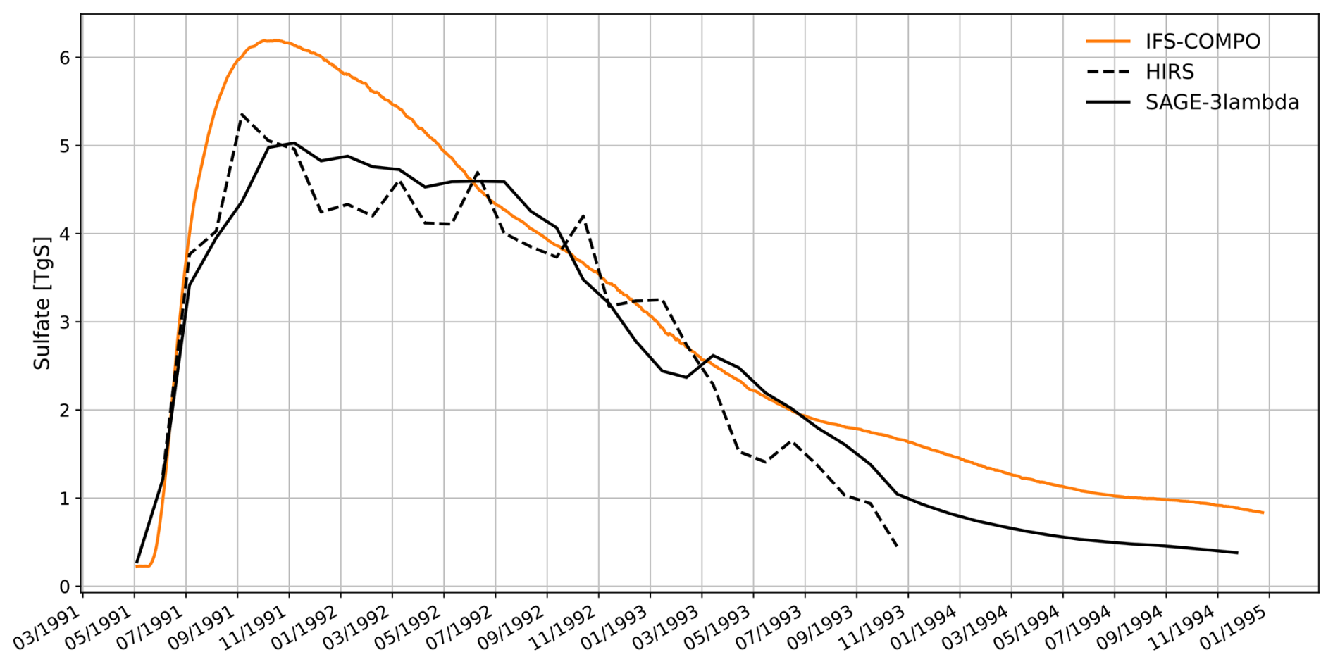
In order to assess the performance of IFS-COMPO in representing the radiative and optical impact of the Pinatubo eruption, Fig. 21 compares the simulated stratospheric aerosol optical depth (AOD) at 550 nm with retrievals and with values taken from the Community Earth System Model (CESM)-Whole Atmosphere Community Climate Model (WACCM) model as provided by Mills et al. (2016). In WACCM, aerosols are represented with a model aerosol scheme following with three lognormal modes (Liu et al., 2012). In general, the representation of stratospheric aerosol and chemistry in WACCM is more complex than in IFS-COMPO. As explained in Sect. 2, values from AVHRR in Fig. 21 are more trustworthy than GloSSAC up to around one year after the eruption (mid 1992), and GloSSAC is relatively more reliable after this. The general patterns in terms of global and tropical simulated stratospheric AOD are quite similar in WACCM and IFS-COMPO.

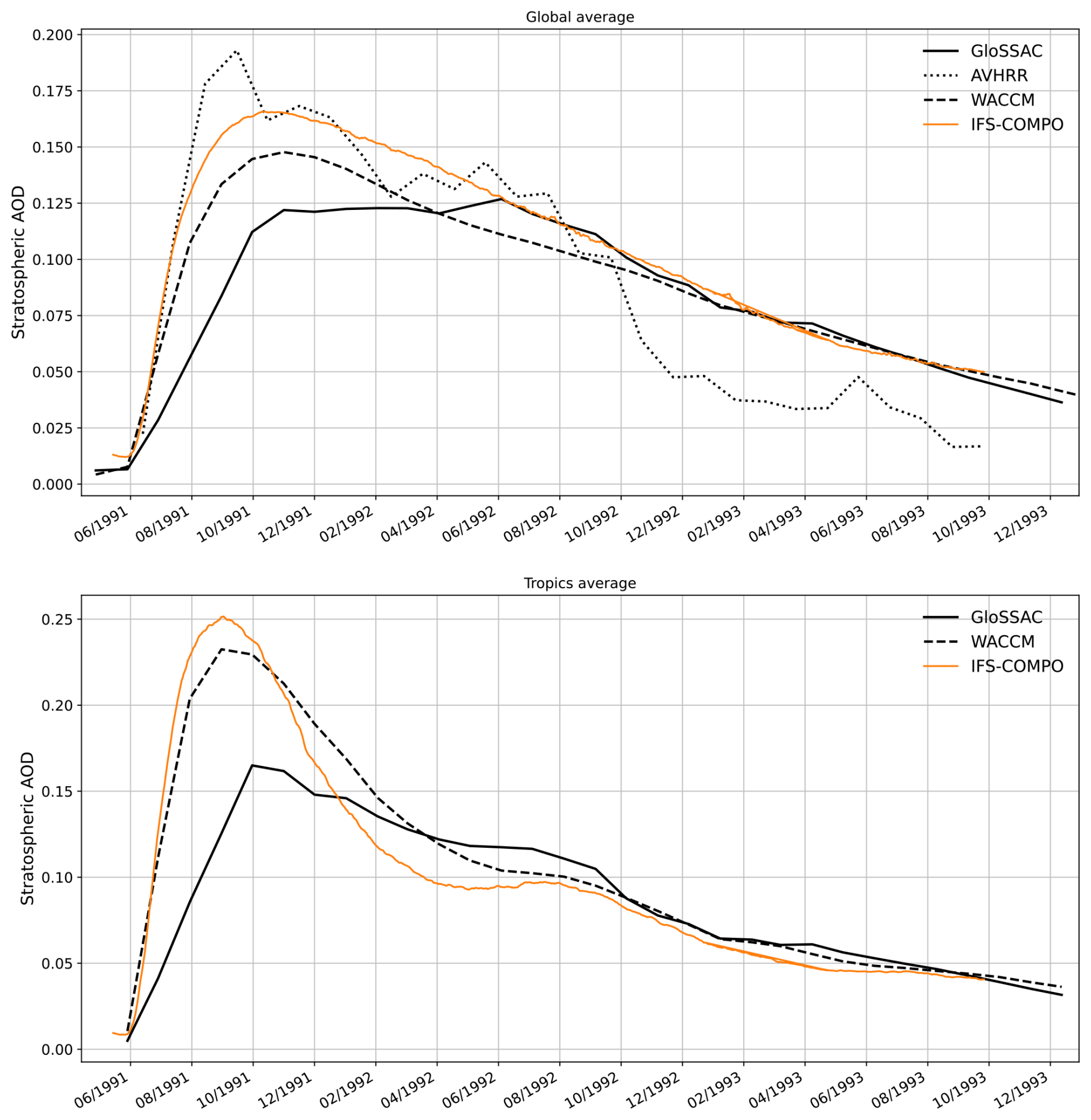
Figure 21 Simulated stratospheric AOD at 550 nm compared against GloSSAC data (AOD at 525 nm) and AVHRR data (AOD at 600 nm). Global value (top) and averaged over the tropics (bottom).

This shows that IFS-COMPO, with a much simpler approach and using a single sulfate tracer, manages to simulate stratospheric AOD with comparable performance to a much more complex scheme which uses 3 aerosol modes. For the global stratospheric AOD, IFS-COMPO shows relatively higher values in the few months after the eruption, with a peak at 0.17 compared to close to 0.15 with WACCM but simulated at the same time. The simulated peak is closer to AVHRR data with IFS-COMPO than with WACCM. The subsequent decrease in stratospheric global AOD is very similar between the two models up to May 1992, when it becomes slightly faster with IFS-COMPO compared to WACCM. After May 1992, the agreement is almost perfect between simulated global stratospheric AOD from IFS-COMPO and the GloSSAC values. The simulated peak in stratospheric AOD is much higher when averaging over the Tropics for both models, reaching 0.25 for IFS-COMPO and 0.23 for WACCM, at about the same time (August 1991). The simulated decrease in stratospheric AOD is faster with IFS than with WACCM, up to June 1992. After that, the two models show a very similar behaviour and are close to GlOSSAC values.

Figure 22 shows a time series of simulated and retrieved aerosol extinctions at 500 nm for both 22 and 30 km altitudes. It should be reminded that the very high values of aerosol extinction just after the eruption are not adequately quantified by GloSSAC (see Sect. 3.1). At 22 km and at 30 km, the broad features of the eruption simulated by the modelling experiment are similar to the ones found in GloSSAC. However the extension of the plume to the Southern Hemisphere (SH) is underestimated and at 30 km, the simulated extinction is slightly overestimated compared to GloSSAC. The underestimation of simulated extinction in the SH could be caused by an inadequate simulated injection height, affecting the subsequent horizontal and vertical transport of the volcanic sulfate plume.

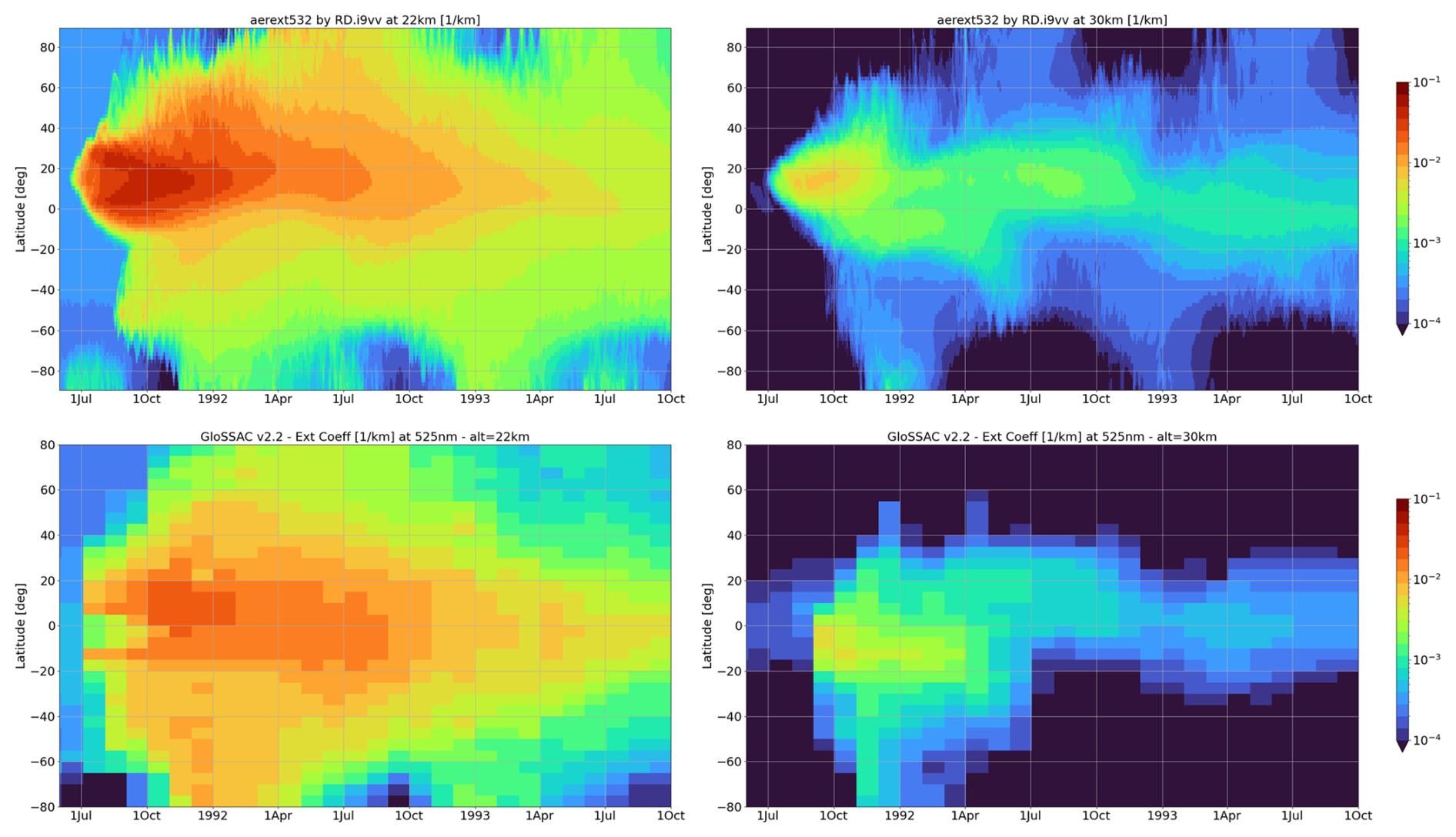
Figure 22 Time-latitude sections of the extinction coefficient around 500 nm (532 nm for IFS, upper panels; 525 nm for GloSSAC, lower panel) at 22 (left) and 30 km (right) altitude for the Pinatubo situation.

The August 1991 Cerro Hudson eruption, which released 2.3 TgSO₂, had an impact on stratospheric aerosol loading which is deeply intertwined with the volcanic burden produced by the Pinatubo eruption. A recent modelling study found a significant contribution of this Cerro Hudson eruption to the simulated aerosol load over the Antarctic (Case et al., 2024). In our simulations, the Cerro Hudson eruption produced a comparatively small amount of sulfate, which may be another cause for the underestimation of simulated extinction. The fact that the co-emission of water vapour is not taken into account could possibly explain this underestimation, or alternatively, the Cerro Hudson injection specifics could be improved.

Figure 23 shows the simulated surface area density (SAD) in June 1992. It should be noted that the SAD shown here is computed from the prognostic sulfate aerosol mass mixing ratio, together with the varying size distributions applied as outlined in Sect. 2.3. The SAD computed from prognostic aerosol information is not yet used to account for the aerosol impact on heterogeneous chemistry reactions. For the Northern hemisphere (NH) and the Tropics, the shapes of the simulated SAD profiles match those provided by GloSSAC quite well, especially in the tropics. In particular, the simulated SAD peak agrees with GloSSAC at altitudes close to 20 km in the NH, and between 20 and 24 km in the tropics. The simulated values exhibit a high bias of nearly 100 % for the NH while for the SH, the simulated SAD is too low below 23 km, which is consistent with the results of the evaluation versus GloSSAC extinction: the extension of the volcanic plume to latitudes below 30° S is underestimated. This could be due, either to a transport issue, or to an inadequate representation of the eruption of the Cerro Hudson on 15 August 1991, which released a significant amount of sulphur dioxide. Above 23 km, similarly to other regions, the simulated SAD is overestimated.

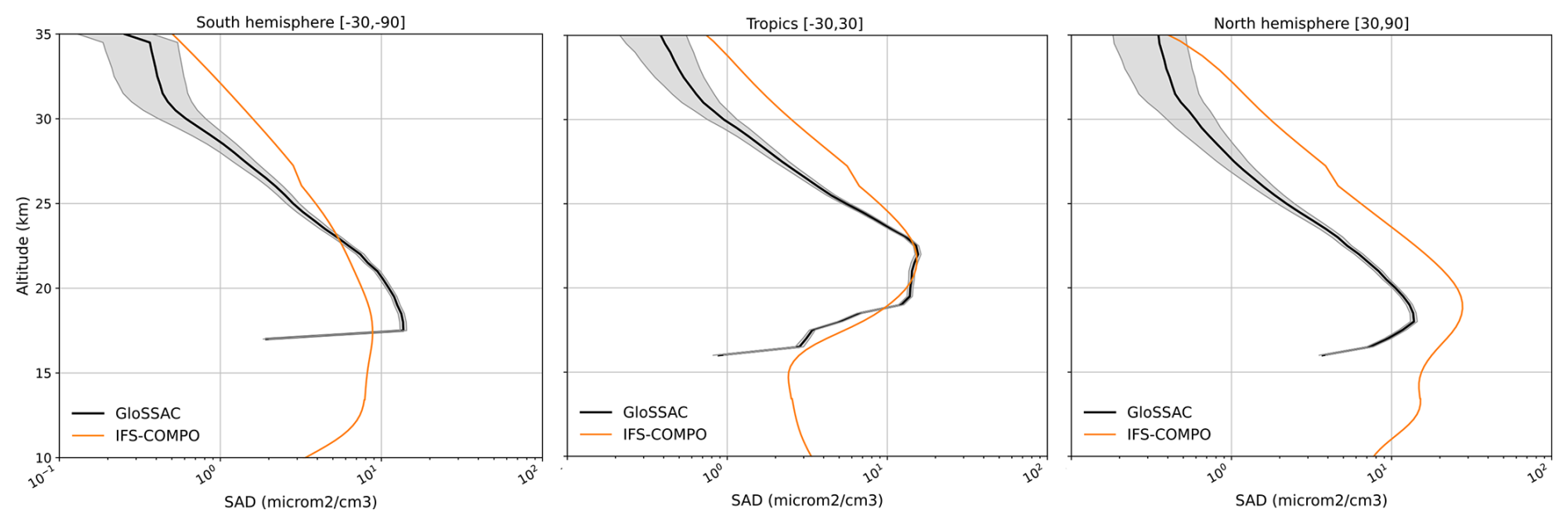
Figure 23 The simulated (blue line) and retrieved SAD (black line) in June 1992 in the extratropical Southern latitudes (left, 90–30° S), Tropics (bottom, 30° S–30° N), and Northern latitudes (right, 30–90° N).

9 Summary and conclusions

Over the past five years, the modelling of stratospheric composition for operational CAMS products has progressed from using a single, climatology-based parameterization of ozone to incorporating a comprehensive description of stratospheric chemistry and sulfate aerosols. We have documented here the two latest cycles of this model, and evaluated the resulting chemical forecasts using mainly limb-scanning satellite observations. This evaluation is expected to be of particular interest in future assessments of aspects related to the stratosphere in the next CAMS reanalysis of atmospheric composition. It comprises three case studies: an 11 month quiescent period (July 2023–May 2024) where global vertical profiles of 10 gaseous species and aerosol extinction coefficients are analysed, including the corresponding model-minus-observation statistics; polar ozone depletion through seven different winter-spring episodes for the same species and two bromine species; and the evolution of the volcanic sulfate aerosol layer during the years following the major Pinatubo eruption of 1991.

A simple representation of the stratospheric sulphur cycle has been implemented in IFS-COMPO Cy49, spanning gaseous and particulate phases. This representation is based on a single tracer that represents both tropospheric and stratospheric particulate sulfate in an integrated way, in order to minimize the computing costs. Despite this limitation, the simple stratospheric aerosol scheme is able to correctly represent the quiescent component of stratospheric aerosol loading, and the broad features of a major volcanic eruption such as the June 1991 Pinatubo eruption, where emissions are prescribed. As such, this development represents a significant and welcome extension of the capabilities of the global CAMS system.

Our evaluation has shown the usefulness of multi-species reanalyses of stratospheric composition, i.e. those which include other species than O₃. We used here the BASCOE Reanalyses of Aura-MLS (BRAM) to initialize chemical forecasts and easily evaluate the evolution of their biases over timescales of 6 months in the Arctic and 9 months in the Antarctic (Sect. 6). Considering the separate evaluation of the operational control runs with no chemical data assimilation (Sect. 5), the need arose to summarize our evaluations. A new scorecard fulfils this need (Sect. 7) and shows that in addition to O₃, the model already delivers good performance for CH₄, N₂O and H₂O – although significant issues are found in the tropical lower stratosphere, especially for water vapour.

The detailed discussions in Sects. 5 and 6 lead us to a process-oriented summary to highlight four areas where future research and developments are needed to improve the performance of IFS-COMPO in the stratosphere:

• Brewer–Dobson Circulation (BDC) and long-range transport. The distribution and variability of the long-lived species CH₄, H₂O and N₂O are well captured, including their temporal variations in the polar lower stratosphere. N₂O is improved by the Cy49R1 upgrade, which we attribute to the activation of the Bermejo–Conde mass fixer in the transport module. However, both CH₄ and N₂O are overestimated in the upper stratosphere, possibly reflecting a possible issue with the BDC resulting from the analyses of the wind fields. Further research is needed to confirm or reject this conjecture, potentially through comparisons with Age of Air datasets or by implementing SF₆ in the BASCOE module of IFS-COMPO.

• Heterogeneous Chemistry. The evaluation of HCl improved notably from Cy48R1 to Cy49R1 because of the update of heterogeneous chemical rates. On the other hand, persisting disagreements in the concentrations of HCl, HNO₃, ClONO₂, and N₂O₅ indicate gaps in the representation of heterogeneous chemistry. At this stage, IFS-COMPO Cy49 does not yet have full interactivity between aerosols and gas-phase composition, since the heterogeneous chemical rates still use a climatology of sulfate aerosols SAD. This feedback will be implemented in the near future and may correct some biases encountered with respect to nitrogen species in the lower stratosphere. Capturing the chlorine activation induced by wildfire aerosol will require accounting for the enhanced solubility of HCl on organic aerosols, and the subsequent heterogeneous reactions of HCl.

• Polar Stratospheric Clouds (PSC). due to its operational aim, IFS-COMPO can not afford to capture the details of PSC microphysics, chemistry and transport. While the current parameterisation only intends to capture their impact on gas-phase composition, it falls short of this target. The depletion of HNO₃ is too intense under polar vortex conditions because the overly simple PSC parameterization attempts to represent denitrification but does not account for gravitational settling. The partial columns of HCl in the polar lower stratosphere are well captured at the beginning and end of each winter-spring season, but they decrease too quickly at the beginning of winter and recover too early i.e., before spring. Since these HCl biases are insensitive to the specific dynamics of each Antarctic winter, this species is a prime target to guide future improvements of PSC-related processes. Future versions of IFS-COMPO should also consider the partitioning of HNO₃ between its gaseous and condensed phases.

• NO_x and O₃ in the upper stratosphere. The overestimation of NO₂ and the ozone deficit in the upper stratosphere remain unresolved issues, which persist in all models using the BASCOE photochemistry module (CTM, GEM-BACH, IFS-COMPO) despite different input meteorological analyses, photolysis configurations, transport algorithms, and initialization details. The causes of these deficits are probably related but remain uncertain and require further research. Progress may hinge on novel comparisons with the scarce observations of OH or HO₂.

IFS-COMPO may never be able to catch up with research models developed specifically to investigate in detail each of these processes. Still, it may prove to be a useful tool for further studies of the couplings between stratospheric aerosols and gas-phase chemistry. The current cycle also paves the way to the assimilation of stratospheric composition observations beyond ozone, in an operational Data Assimilation System developed primarily for Numerical Weather Forecasting. This will enable the operational monitoring and forecasting of stratospheric composition, including during exceptional events such as major volcanic eruptions.