A new hybrid particle-puff approach to atmospheric dispersion modeling, implemented in the Danish Emergency Response Model of the Atmosphere (DERMA)

The Danish Emergency Response Model of the Atmosphere (DERMA) is a Lagrangian puff model originally developed for long-range dispersion modeling, at distances longer than roughly 50 km from the source. The model is used operationally as part of Danish emergency preparedness for the prediction of atmospheric dispersion in case of nuclear accidents, airborne spread of animal diseases, and ash from volcanic eruptions. To be able to simulate dispersion on shorter spatial scales, a new description of turbulent diffusion has been developed and implemented in DERMA, combining a stochastic particle approach with a classic puff model. Furthermore, updates have been made to the parameterizations of the turbulent wind fluctuations and Lagrangian timescales, the boundary layer height, and the initial plume rise due to heat release. These improvements allow a more realistic description of turbulent diffusion near the release location, while an updated version of the existing turbulence description is used at longer distances. The new version of DERMA is evaluated against three different tracer gas experiments: the European Tracer Experiment (ETEX), the Øresund experiment, and the Kincaid experiment. The results indicate that the new particle-puff hybrid approach gives more accurate predictions, especially on shorter spatial scales, while a small improvement is also observed for long-range dispersion.

1 Introduction

Lagrangian atmospheric dispersion models can be divided into two categories, stochastic particle models and puff models. Both rely on modeling the positions of particles following Lagrangian trajectories. In stochastic particle models, each particle follows a turbulent trajectory estimated using stochastic differential equations, and the resulting concentration field is then determined by the spread of particles. These models typically make as few assumptions as possible; therefore, they are capable of making physically accurate simulations. However, a large number of particles is needed to accurately resolve the fine structures of the three-dimensional plume, which makes this type of model computationally expensive. Furthermore, as discussed by Stohl et al. (2005), short advection time steps, on the order of a few seconds, may be necessary in order to resolve the turbulent trajectories in all conditions. Some examples of stochastic particle models are the models FLEXPART (Stohl et al., 2005; Pisso et al., 2019), HYSPLIT (Draxler and Hess, 1997), and NAME (Jones et al., 2004). The latter uses a hybrid particle-puff description for short-range modeling, while the particles are only assumed to be point concentrations at longer distances (Jones et al., 2004).

The Lagrangian puff approach is a computationally cheaper alternative, where each puff instead follows the average wind field, and turbulent diffusion is assumed to follow a Gaussian distribution locally around each puff's centroid. Some examples are CALPUFF (Scire et al., 2000), DIPCOT (Andronopoulos et al., 2009), RIMPUFF (Thykier-Nielsen et al., 1999), and the Danish Emergency Response of Model of the Atmosphere (DERMA) (Sørensen et al., 2007). In this type of model, much fewer particles are used compared to the stochastic particle models, and the Gaussian concentration distributions then “fill the gaps” between particle locations. For relatively young puffs, this assumption works quite well, but when the puffs grow beyond a certain size, the vertical wind shear may cause puffs to stretch over different flow regimes, which would in reality distort the Gaussian shape (Jones et al., 2004). A typical solution for this problem, e.g., used in NAME, CALPUFF, and RIMPUFF, is the use of puff splitting; i.e., a puff that grows too large is split into several smaller puffs at different heights (Jones et al., 2004; Scire et al., 2000; Thykier-Nielsen et al., 1999). This ensures a more physical behavior, but it introduces new challenges due to the continuously increasing number of puffs (Draxler and Hess, 1997). An alternative approach, described further below, is to introduce stochastic movement, which exposes each puff to the wind at different heights and thereby leads to a more realistic dispersion pattern.

In addition to these two model types, different hybrid formulations have been proposed combining elements from both stochastic particle models and puff models. As already mentioned, the NAME model employs such an approach on shorter scales, but the models DIPCOT and DERMA also combine the puff approach with a stochastic displacement of puffs (Andronopoulos et al., 2009; Sørensen et al., 2007). Another example of a hybrid formulation is the Puff-Particle Model (PPM) suggested by De Haan and Rotach (1998). In the PPM, the turbulent effects are separated into two distinct physical processes, a meandering part (larger scale than the puff) and a relative dispersion around each puff centroid, represented by the puff growth. However, in order to keep puffs smaller than the meandering scales, PPM uses more puffs and more frequent puff splitting than in regular puff models and should be considered a compromise between the two model types, with respect to both accuracy and efficiency (De Haan and Rotach, 1998).

In the currently operational version of DERMA, v1.0.0, complete mixing throughout the boundary layer is assumed, which means that the concentration field of a puff is only assumed Gaussian horizontally, while it is described by a uniform distribution vertically for puffs inside the planetary boundary layer (PBL). Thus, as discussed above, the puffs in DERMA are likely to stretch over different flow regimes. However, a vertical stochastic transport scheme inside the PBL is used as an alternative to puff splitting; by randomly moving puff centroids inside the PBL to new vertical positions, each puff is exposed to the vertical wind shear over time (Sørensen, 1998; Sørensen et al., 2007). Despite this relatively simple formulation, DERMA was ranked as one of the best-performing models in the European Tracer Experiment (ETEX) model evaluation (Graziani et al., 1998).

DERMA is currently used operationally for a number of purposes for Danish emergency preparedness, including nuclear accidents, volcanic eruptions, and airborne animal diseases (Sørensen et al., 2000, 2001; Mikkelsen et al., 2003; Gloster et al., 2010; Hoe et al., 2002). In recent years, the model has further been used in different research projects about inverse modeling for source localization and source term reconstruction for a nuclear accident (Sørensen, 2018; Tølløse et al., 2021; Tølløse and Sørensen, 2022). DERMA was specifically designed for long-range dispersion modeling, and some assumptions are not applicable on shorter scales. The aim of this study is to develop a new description of turbulent diffusion, which enables the new version of the model, DERMA v2.0.0, to accurately predict dispersion closer to the release location.

In this study, we develop a new hybrid particle-puff approach, which separates the turbulent diffusion into a stochastic part and a puff part. On shorter scales, the separation is based on the size of the puff compared to the length scale associated with the largest turbulent eddies. This is conceptually similar to the approach by De Haan and Rotach (1998) used in the PPM. However, on longer scales, the stochastic part works as compensation for the fact that the puff assumption fails for physically large puffs, similar to the formulation in DERMA v1.0.0. In addition to the new description of turbulent diffusion, several updates have been made to DERMA, which are described in detail in Sect. 2. Furthermore, the new particle-puff approach has been evaluated against three tracer gas experiments: the European Tracer Experiment (ETEX), the Øresund experiment, and the Kincaid experiment. Details on the evaluation process and the results are presented in Sect. 3. Finally, a summary and the conclusions are presented in Sect. 4.

2 Model description

In this section, a detailed description of all the new elements in DERMA is given. For a more general description of DERMA, see Sørensen (1998), Baklanov and Sørensen (2001), and Sørensen et al. (2007). In Sect. 2.1, the new hybrid particle-puff formulation is described. Next, Sect. 2.2 describes the updates made to the PBL parameterization, including a new parameterization of turbulent wind fluctuations, Lagrangian timescales, and PBL height. Finally, Sect. 2.3 describes the Concawe and Briggs plume rise algorithms, which have also been implemented.

2.1 Hybrid particle-puff description

As discussed previously, one of the shortcomings of the puff model approach is that puffs will eventually grow larger than the characteristic length scale of the vertical wind shear, causing the puff assumption to fail. Furthermore, the smallest puffs may be smaller than the largest turbulent eddies in some conditions. Therefore, at the early stages, the puffs should be displaced by these, until they grow larger than the eddies themselves. In this study, we develop a simple hybrid approach, which attempts to target both of these issues. For small puffs, the hybrid approach is designed such that puffs are displaced by the largest eddies, while smaller eddies cause the puffs to grow, and, for large puffs, a stochastic displacement will expose puffs to the wind shear, hence avoiding the need for puff splitting.

As in DERMA v1.0.0, the puffs grow according to the formulation by Gifford (1984),

$$\begin{array}{}\text{(1)}& {\mathit{\sigma }}_i^{\mathrm{2}}=\mathrm{2}{K}_i{t}_{L_{u_i}}\left\{{\mathit{\tau }}_i-\left(\mathrm{1}-e^{-{\mathit{\tau }}_i}\right)-{\displaystyle \frac{\mathrm{1}}{\mathrm{2}}}{\left(\mathrm{1}-e^{-{\mathit{\tau }}_i}\right)}^{\mathrm{2}}\right\},\end{array}$$

where σ_i is the puff's standard deviation along the x_i axis; K_i is the turbulent diffusivity; $t_{L_{u_i}}$ is the Lagrangian timescale, i.e., the auto-correlation time for the velocity fluctuations; t is the age of the puff; and ${\mathit{\tau }}_i=t/t_{L_{u_i}}$. In DERMA v2.0.0, we instead consider the time derivative of Eq. (1),

$${\displaystyle \frac{\partial }{\partial t}}{\mathit{\sigma }}_i^{\mathrm{2}}=\mathrm{2}{\mathit{\sigma }}_{u_i}^{\mathrm{2}}{t}_{L_{u_i}}{\left(\mathrm{1}-e^{-{\mathit{\tau }}_i}\right)}^{\mathrm{2}},$$

where we have used the relation between the diffusivity and the turbulent velocity scale $K_i={\mathit{\sigma }}_{u_i}^{\mathrm{2}}{t}_{L_{u_i}}$. This can be written in the numerical form

$$\begin{array}{ll}{\displaystyle }\mathrm{\Delta }{\mathit{\sigma }}_i^{\mathrm{2}}(t+\mathrm{\Delta }t/\mathrm{2})=& {\displaystyle }\mathrm{2}{\mathit{\sigma }}_{u_i}^{\mathrm{2}}\left(t\right)t_{L_{u_i}}\left(t\right)\\ \text{(2)}& {\displaystyle }& {\displaystyle }\times \mathrm{\Delta }t{\left(\mathrm{1}-\text{exp}\left(-{\displaystyle \frac{t+\mathrm{\Delta }t/\mathrm{2}}{t_{L_{u_i}}\left(t\right)}}\right)\right)}^{\mathrm{2}},\end{array}$$

which is evaluated at the time $t+\mathrm{\Delta }t/\mathrm{2}$, i.e., halfway between the two neighboring discrete time steps. To avoid double-counting the effects of turbulence, Eq. (2) must describe the combined effects of the puff growth and stochastic parts of the turbulent diffusion.

We consider the case where puffs have been dispersed around a point following mean wind trajectories x_t and assume that the puff centroids, x_p, are distributed according to Gaussian particle distributions in all three spatial dimensions. Thus, along the x_i axis, puff centroids are distributed as $f\left(x_i\right)=\mathcal{N}(x_{i,\mathrm{t}},{\mathit{\sigma }}_{i,\text{part}})$. Furthermore, the concentration field from each puff around its centroid is assumed to follow the Gaussian distribution $g\left(x_i\right)=\mathcal{N}(\mathrm{0},{\mathit{\sigma }}_{i,\text{puff}})$.

The resulting concentration distribution can be obtained by calculating the convolution of the two distributions (Bromiley, 2003),

$$\begin{array}{ll}{\displaystyle }f\left(x_i\right)⊛g\left(x_i\right)& {\displaystyle }=\underset{-\mathrm{\infty }}{\overset{\mathrm{\infty }}{\int }}f\left(x_i^{\prime }\right)g(x_i-x_i^{\prime })\mathrm{d}{x}_i^{\prime }\\ {\displaystyle }& {\displaystyle }=\mathcal{N}\left(x_{i,\mathrm{t}},\sqrt{{\mathit{\sigma }}_{i,\text{part}}^{\mathrm{2}}+{\mathit{\sigma }}_{i,\text{puff}}^{\mathrm{2}}}\right).\end{array}$$

Next, we impose the requirement that the resulting concentration distribution should be identical to the Gaussian distribution $\mathcal{N}(x_{i,\mathrm{t}},{\mathit{\sigma }}_i)$, with σ_i from Eq. (1), in accordance with the formulation by Gifford (1984). To ensure this, the increment of the variances for the distributions f(x_i) and g(x_i) must fulfill the following requirements at every numerical time step

$$\begin{array}{ll}{\displaystyle }\mathrm{\Delta }{\mathit{\sigma }}_{i,\text{puff}}^{\mathrm{2}}& {\displaystyle }={\mathit{\beta }}_i^{\mathrm{2}}\mathrm{\Delta }{\mathit{\sigma }}_i^{\mathrm{2}},\\ \text{(3)}& {\displaystyle }\mathrm{\Delta }{\mathit{\sigma }}_{i,\text{part}}^{\mathrm{2}}& {\displaystyle }=(\mathrm{1}-{\mathit{\beta }}_i^{\mathrm{2}})\mathrm{\Delta }{\mathit{\sigma }}_i^{\mathrm{2}},\end{array}$$

where $\mathrm{\Delta }{\mathit{\sigma }}_i^{\mathrm{2}}$ is given by Eq. (2) and ${\mathit{\beta }}_i\in [\mathrm{0},\mathrm{1}]$ is a parameter determining how much stochastic movement is used. If β_i = 1, the model is a classical puff model, while, if β_i=0, the turbulent diffusion is described purely by the stochastic transport and the puffs keep their initial sizes.

The indices _i,part and _i,puff indicate the parts of the turbulence accounted for by stochastic displacement and puff growth along the x_i axis, respectively. Hence, during each numerical time step, a puff's variance grows with $\mathrm{\Delta }{\mathit{\sigma }}_{i,\text{puff}}^{\mathrm{2}}$, Eq. (3), while its centroid is moved by a random walk with step size Δσ_i,part, Eq. (3). If the turbulence is Gaussian and if there is no vertical wind shear, any value of β_i should be valid, provided there is a sufficient number of particles. However, since vertical wind shear is a fundamental feature of the atmosphere, especially in the PBL, the addition of a stochastic element to the turbulence description should improve the performance by exposing puffs to the winds at different heights.

2.1.1 Determining β_i

Early in the life of a puff, the puff might be smaller than the largest turbulent eddies; therefore, we can make a physical distinction between the particle part and the puff part. Although our approach is different, this distinction is conceptually similar to the approach by De Haan and Rotach (1998). Here, we use the fraction of the turbulent kinetic energy (TKE) on larger scales than the puff itself. Thus, we first consider the TKE spectrum: (Kolmogorov, 1941)

$$\begin{array}{}\text{(4)}& \text{TKE}\left(k\right)\propto {\mathit{\epsilon }}^{\mathrm{2}/\mathrm{3}}{k}^{-\mathrm{5}/\mathrm{3}},\end{array}$$

where ε is the TKE dissipation rate, $k=\frac{\mathrm{2}\mathit{\pi }}{\mathit{\lambda }}$ is the wave number, and the wavelength λ corresponds to the length scale associated with the turbulent eddies. In reality, k=|k|, where k is the three-dimensional wave number, which is of course not necessarily equal in all physical dimensions. However, for this purpose, we assume that the relation Eq. (4) holds in each spatial dimension individually. Thus, assuming that the puff has the spatial extent σ_i along the x_i axis, we can estimate the fraction of the TKE accounted for by eddies on smaller spatial scales than the puff itself.

$$\begin{array}{}\text{(5)}& {\displaystyle \frac{{\text{TKE}}_{\text{puff}}}{\text{TKE}}}={\displaystyle \frac{{\int }_{\frac{\mathrm{2}\mathit{\pi }}{{\mathit{\sigma }}_i}}^{\mathrm{\infty }}\text{TKE}\left(k_i\right)\mathrm{d}{k}_i}{{\int }_{\frac{\mathrm{2}\mathit{\pi }}{l_i}}^{\mathrm{\infty }}\text{TKE}\left(k_i\right)\mathrm{d}{k}_i}}={\left({\displaystyle \frac{{\mathit{\sigma }}_i}{l_i}}\right)}^{\mathrm{2}/\mathrm{3}},\end{array}$$

where l_i is the length scale associated with the largest eddies along the ith physical dimension, which is estimated as $l_i={\mathit{\sigma }}_{u_i}{t}_{L_{u_i}}$.

The fraction in Eq. (5) seems like a natural choice for the value of ${\mathit{\beta }}_i^{\mathrm{2}}$, except that, when the puff grows larger than the largest eddies, the particle part will then naturally die out. Thus, to ensure that the stochastic part does not vanish, we define

$$\begin{array}{}\text{(6)}& {\mathit{\beta }}_i=\text{max}\left({\mathit{\beta }}_{\text{min}},{\left({\displaystyle \frac{{\mathit{\sigma }}_i}{l_i}}\right)}^{\mathrm{1}/\mathrm{3}}\right),\end{array}$$

where ${\mathit{\beta }}_{\text{min}}\in [\mathrm{0},\mathrm{1}]$ is a hyperparameter that needs to be determined to find the ideal balance between the particle and puff parts. We use ${\mathit{\beta }}_{\text{min}}=\sqrt{\mathrm{1}/\mathrm{2}}$, which divides the turbulence evenly between the particle part and the puff part.

It is assumed that puffs inside the boundary layer are reflected both at the surface and at the PBL top. Furthermore, for puffs above the boundary layer, the stochastic part will automatically be turned off by setting β_i=1.

2.1.2 Short-range and long-range formulations

The concentration field from a puff in a point $(x_{\mathrm{p}},y_{\mathrm{p}},z_{\mathrm{p}})$ can be written as

$$\begin{array}{}\text{(7)}& {\displaystyle }\begin{array}{rl}& C_{\mathrm{p}}={\displaystyle \frac{Q_{\mathrm{p}}}{\mathrm{2}\mathit{\pi }{\mathit{\sigma }}_y^{\mathrm{2}}{\mathit{\sigma }}_z}}\\ & \times \text{exp}\left\{-{\displaystyle \frac{\mathrm{1}}{\mathrm{2}}}{\left({\displaystyle \frac{x-x_{\mathrm{p}}}{{\mathit{\sigma }}_y}}\right)}^{\mathrm{2}}-{\displaystyle \frac{\mathrm{1}}{\mathrm{2}}}{\left({\displaystyle \frac{y-y_{\mathrm{p}}}{{\mathit{\sigma }}_y}}\right)}^{\mathrm{2}}s-{\displaystyle \frac{\mathrm{1}}{\mathrm{2}}}{\left({\displaystyle \frac{z-z_{\mathrm{p}}}{{\mathit{\sigma }}_z}}\right)}^{\mathrm{2}}\right\},\end{array}\end{array}$$

where Q_p is the mass/activity carried by the puff. However, when a puff has grown to a certain size compared to the PBL height, a uniform distribution is assumed vertically; i.e., the formulation from DERMA v1.0.0 is adapted. This happens whenever ${\mathit{\sigma }}_z\ge h/\mathit{\alpha }$ , where h is the PBL height and α is a hyperparameter determining how fast a puff is assumed to fill out the boundary layer. We use α=2, which means that complete mixing is assumed when 2σ_z exceeds the PBL height. The reasoning behind this is that, at this stage, the Gaussian distribution is already sufficiently diluted such that the surface concentrations are not expected to change dramatically by changing to the uniform distribution.

Whenever a puff fulfills this requirement, the concentration field is instead described by

$$\begin{array}{ll}{\displaystyle }& {\displaystyle }{C}_{\mathrm{p}}={\displaystyle \frac{Q_{\mathrm{p}}}{\mathrm{2}\mathit{\pi }{\mathit{\sigma }}_y^{\mathrm{2}}h}}\text{exp}\left\{-{\displaystyle \frac{\mathrm{1}}{\mathrm{2}}}{\left({\displaystyle \frac{x-x_{\mathrm{p}}}{{\mathit{\sigma }}_y}}\right)}^{\mathrm{2}}-{\displaystyle \frac{\mathrm{1}}{\mathrm{2}}}{\left({\displaystyle \frac{y-y_{\mathrm{p}}}{{\mathit{\sigma }}_y}}\right)}^{\mathrm{2}}\right\}\mathit{\delta }(z,h),\\ \text{(8)}& {\displaystyle }& {\displaystyle }\text{where}\mathit{\delta }(z,h)=\left\{\begin{array}{ll}\mathrm{1}& \text{ if }z\le h\\ \mathrm{0}& \text{ if }z>h\end{array}\right..\end{array}$$

This concept is illustrated in Fig. 1, where a schematic drawing shows the behavior of the model at short and long scales. This formulation will naturally result in a sharp change in concentration at the top of the boundary layer, which is especially suitable for convective conditions with a capping inversion trapping particles inside the PBL. For stable conditions, the formulation may be less accurate, but, as described below, different processes allow puffs to escape the PBL, resulting in a smoother transition at the top of the PBL.

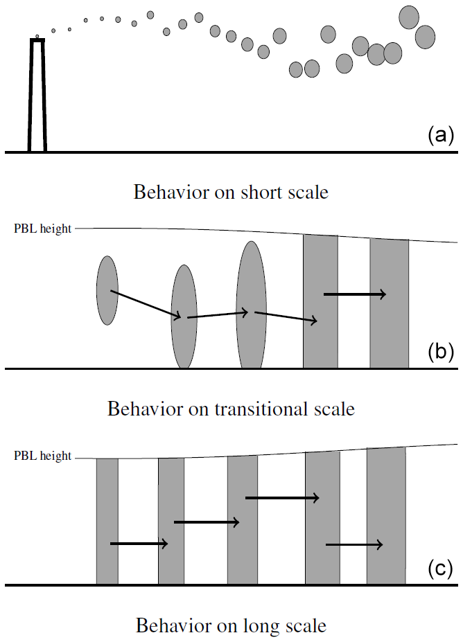
Figure 1 Illustration of the formulation used in DERMA v2.0.0. Panel (a) shows how puffs are released from the top of a stack and are randomly displaced vertically. Panel (b) shows the transition when a puff starts using a uniform concentration distribution in the vertical direction. Finally, panel (c) shows how the long-range formulation works; puffs assume a uniform vertical distribution inside the PBL, and the height of the puff centroid is displaced vertically with the stochastic transport scheme.

When the complete mixing state is reached, the puff is assumed to fill out the boundary layer at all later times, even when the boundary layer grows. Thus, since the puff is no longer growing vertically, all turbulence is assumed to contribute to the stochastic movement; i.e., we set β_z=0. Only if the centroid of a completely mixed puff escapes the boundary layer, will it transform back to a Gaussian form in the vertical dimension. The leakage of concentration to the free troposphere can happen in two different ways: (1) if a puff centroid is lifted sufficiently by the mean wind or (2) if the boundary layer shrinks and, as a result, a puff centroid happens to be above the boundary layer.

This long-range formulation is similar to that of DERMA v1.0.0 but with the improved stochastic transport scheme described above, whereas the old stochastic transport scheme simply assigns a new random height to each puff inside the PBL at every time step (Sørensen et al., 2007).

2.2 Parameterization of boundary layer parameters

The calculation of both the puff part and the particle part described above depends on ${\mathit{\sigma }}_{u_i}^{\mathrm{2}}$ and $t_{L_{u_i}}$, which in turn depend on several boundary layer parameters that are either imported or calculated in DERMA.

From the output of the numerical weather prediction (NWP) model, DERMA imports instantaneous turbulent fluxes of momentum, τ₀, and sensible and latent heat, Q_s and Q_l. From these, the following parameters are calculated (Zannetti, 2013, Chap. 3):

$$\begin{array}{}\text{(9)}& {\displaystyle }L& {\displaystyle }=-{\displaystyle \frac{u_{*}^{\mathrm{3}}{T}_{\mathrm{v}}}{\mathit{\kappa }g{\left(\stackrel{\mathrm{‾}}{w^{\prime }{\mathit{\theta }}_{\mathrm{v}}^{\prime }}\right)}_{\mathrm{0}}}},\text{(10)}& {\displaystyle }{u}_{*}& {\displaystyle }=\sqrt{{\displaystyle \frac{{\mathit{\tau }}_{\mathrm{0}}}{\mathit{\rho }}}},\text{(11)}& {\displaystyle }{w}_{*}& {\displaystyle }={\left({\displaystyle \frac{hg{\left(\stackrel{\mathrm{‾}}{w^{\prime }{\mathit{\theta }}_{\mathrm{v}}^{\prime }}\right)}_{\mathrm{0}}}{T_{\mathrm{v}}}}\right)}^{\mathrm{1}/\mathrm{3}},\end{array}$$

where L is the Obukhov length, which is related to the static stability of the boundary layer, and the friction velocity u_* is assumed the fundamental velocity scale of the non-convective turbulent boundary layer, whereas w_* is the convective velocity scale. Furthermore, ρ is the air density, g = 9.81 m s⁻² is the gravitational acceleration constant, κ=0.4 is the von Karman constant, T_v is the surface virtual temperature, and h is the PBL height, which is calculated as described in Sect. 2.2.1. Finally, $(\stackrel{\mathrm{‾}}{w^{\prime }{\mathit{\theta }}_{\mathrm{v}}^{\prime }}{)}_{\mathrm{0}}$ is the surface buoyancy flux, i.e., the flux of virtual potential temperature, which can be estimated directly from the imported heat fluxes as $(\stackrel{\mathrm{‾}}{w^{\prime }{\mathit{\theta }}_{\mathrm{v}}^{\prime }}{)}_{\mathrm{0}}\approx (Q_{\mathrm{s}}+\mathrm{0.07}{Q}_{\mathrm{l}})/(\mathit{\rho }{c}_{\mathrm{p}})$, where c_p is the heat capacity at constant pressure (Zannetti, 2013, Chap. 3).

2.2.1 PBL height

The PBL height parameterization is based on the approach by Vogelezang and Holtslag (1996), which relies on a modified form of the Bulk Richardson number:

$$\begin{array}{}\text{(12)}& Ri\left(z\right)={\displaystyle \frac{(g/{\mathrm{\Theta }}_{\text{v,s}})\left({\mathrm{\Theta }}_{\mathrm{v}}\right(z)-{\mathrm{\Theta }}_{\text{v,s}})z}{U(z{)}^{\mathrm{2}}+V(z{)}^{\mathrm{2}}+\mathrm{100}{u}_{*}^{\mathrm{2}}}},\end{array}$$

where Θ_v,s is the surface virtual potential temperature, Θ_v(z) is the virtual potential temperature at height z, and U(z) and V(z) are the horizontal wind components at height z. The PBL height h is set equal to the height z where the requirement Ri(z)=0.25 is obtained for the first time moving upwards from the ground.

2.2.2 Turbulent wind fluctuations

As in DERMA v1.0.0, the constant turbulent diffusivity $K_y=\mathrm{6}\times {\mathrm{10}}^{\mathrm{3}}$ m² s⁻¹ and corresponding Lagrangian timescale $t_{L_v}={\mathrm{10}}^{\mathrm{4}}$ s are assumed for the horizontal diffusion (Sørensen et al., 2007). The vertical component of turbulent velocity fluctuations and the corresponding Lagrangian timescale are parameterized according to the formulations by Hanna (1984). The formulas are given below for the different stability regimes and are valid for puffs within the PBL. For puffs above the boundary layer, we instead use the constant values σ_w=0.1 m s⁻¹ and $t_{L_w}=\mathrm{100}$ s, resulting in a vertical diffusivity of K_z=1 m² s⁻¹, which was used in the previous version of DERMA and is similar to other models, such as NAME, which uses K_z=1.5 m² s⁻¹ for the free troposphere (Sørensen, 1998; Jones et al., 2004). In the following, z is the particle's height above the ground, and $f={\mathrm{10}}^{-\mathrm{4}}$ s⁻¹ is the Coriolis parameter, assumed constant with the typical value valid for mid-latitudes.

Stable conditions

$$\begin{array}{}\text{(13)}& {\displaystyle }{\mathit{\sigma }}_w& {\displaystyle }=\mathrm{1.3}{u}_{*}\left(\mathrm{1}-{\displaystyle \frac{z}{h}}\right)\text{(14)}& {\displaystyle }{t}_{L_w}& {\displaystyle }=\mathrm{0.1}{\displaystyle \frac{h}{{\mathit{\sigma }}_w}}{\left({\displaystyle \frac{z}{h}}\right)}^{\mathrm{0.8}}\end{array}$$

Neutral conditions

$$\begin{array}{}\text{(15)}& {\displaystyle }{\mathit{\sigma }}_w& {\displaystyle }=\mathrm{1.3}{u}_{*}\text{exp}\left(-\mathrm{2}{\displaystyle \frac{fz}{u_{*}}}\right)\text{(16)}& {\displaystyle }{t}_{L_w}& {\displaystyle }={\displaystyle \frac{\mathrm{0.5}z/{\mathit{\sigma }}_w}{\mathrm{1}+\mathrm{15}fz/u_{*}}}\end{array}$$

Unstable conditions

If $\frac{z}{h}<\mathrm{0.03}$,

$$\begin{array}{}\text{(17)}& {\displaystyle \frac{{\mathit{\sigma }}_w}{w_{*}}}=\mathrm{0.96}{\left(\mathrm{3}{\displaystyle \frac{z}{h}}-{\displaystyle \frac{L}{h}}\right)}^{\mathrm{1}/\mathrm{3}}.\end{array}$$

If $\mathrm{0.03}\le \frac{z}{h}<\mathrm{0.4}$,

$$\begin{array}{}\text{(18)}& {\displaystyle \frac{{\mathit{\sigma }}_w}{w_{*}}}=\text{min}\left[\mathrm{0.96}{\left(\mathrm{3}{\displaystyle \frac{z}{h}}-{\displaystyle \frac{L}{h}}\right)}^{\mathrm{1}/\mathrm{3}},\mathrm{0.763}{\left({\displaystyle \frac{z}{h}}\right)}^{\mathrm{0.175}}\right].\end{array}$$

If $\mathrm{0.4}\le \frac{z}{h}<\mathrm{0.96}$,

$$\begin{array}{}\text{(19)}& {\displaystyle \frac{{\mathit{\sigma }}_w}{w_{*}}}=\mathrm{0.722}{\left(\mathrm{1}-{\displaystyle \frac{z}{h}}\right)}^{\mathrm{0.207}}.\end{array}$$

If $\mathrm{0.96}\le \frac{z}{h}<\mathrm{1}$,

$$\begin{array}{}\text{(20)}& {\displaystyle \frac{{\mathit{\sigma }}_w}{w_{*}}}=\mathrm{0.37}.\end{array}$$

If $\frac{z}{h}<\mathrm{0.1}\text{ and }z>-L$,

$$\begin{array}{}\text{(21)}& t_{L_w}={\displaystyle \frac{\mathrm{0.1}z}{{\mathit{\sigma }}_w[\mathrm{0.55}-\mathrm{0.38}z/L]}}.\end{array}$$

If $\frac{z}{h}<\mathrm{0.1}\text{ and }z\le -L$,

$$\begin{array}{}\text{(22)}& t_{L_w}=\mathrm{0.59}{\displaystyle \frac{z}{{\mathit{\sigma }}_w}}.\end{array}$$

If $\frac{z}{h}\ge \mathrm{0.1}$,

$$\begin{array}{}\text{(23)}& t_{L_w}=\mathrm{0.15}{\displaystyle \frac{h}{{\mathit{\sigma }}_w}}\left[\mathrm{1}-\text{exp}\left(-\mathrm{5}{\displaystyle \frac{z}{h}}\right)\right].\end{array}$$

2.3 Plume rise algorithm

Two different plume rise algorithms have been implemented in DERMA: the Concawe formula and the Briggs formula. The former has the advantage that it is compatible with the current operational setup of DERMA, while the latter takes into account more meteorological considerations. A good overview and a comparison of the algorithms are given by Korsakissok and Mallet (2009). All quantities in the equations below are in SI units.

2.3.1 Concawe formula

The Concawe formula only takes the heat release as input and is therefore more general than the Briggs formulas described below. Furthermore, its formulation makes it particularly interesting in the context of DERMA, because it can be directly implemented in the current operational setup. The plume rise Δh is calculated as (Brummage, 1968)

$$\begin{array}{}\text{(24)}& \mathrm{\Delta }h=\mathrm{0.071}{\displaystyle \frac{Q_{\mathrm{h}}^{\mathrm{0.55}}}{U^{\mathrm{0.67}}}},\end{array}$$

where Q_h is the heat release and U is the model's horizontal wind speed at the height of the release, i.e., the stack height z_s. In the Kincaid experiment, however, the heat release needs to be calculated from the measurements of the exhaust velocity v_g, the gas temperature T_g, and the temperature of the ambient air T. The heat release is calculated as (Korsakissok and Mallet, 2009)

$$\begin{array}{}\text{(25)}& Q_{\mathrm{h}}=\mathrm{228.19}{v}_{\mathrm{g}}{d}_{\mathrm{s}}^{\mathrm{2}}(T_{\mathrm{g}}-T),\end{array}$$

where d_s is the stack diameter.

2.3.2 Briggs formulas

The Briggs formulas are specifically developed for gas being exhausted from a stack; therefore both the exhaust velocity and the gas temperature are considered explicitly. Furthermore, different formulations are used for different stability conditions. The formulas presented here are from Briggs (1965).

Firstly, the static stability parameter s_p and the initial buoyancy flux parameter F_b are defined:

$$\begin{array}{}\text{(26)}& s_{\mathrm{p}}={\displaystyle \frac{g}{T}}{\displaystyle \frac{\mathrm{d}\mathrm{\Theta }}{\mathrm{d}z}},F_{\mathrm{b}}=g{v}_{\mathrm{g}}{d}_{\mathrm{s}}^{\mathrm{2}}{\displaystyle \frac{T_{\mathrm{g}}-T}{T_{\mathrm{g}}}},\end{array}$$

where g is the gravitational acceleration constant and $\mathrm{d}\mathrm{\Theta }/\mathrm{d}z$ is the gradient of the mean potential temperature. Since the algorithm is implemented in DERMA, the ambient air temperature T is the model temperature here instead of the observed temperature as used for calculation of Q_h in Eq. (25).

In all cases, the plume rise is given by

$$\begin{array}{}\text{(27)}& \mathrm{\Delta }h=\text{min}(\mathrm{\Delta }{h}_{\mathrm{1}},\mathrm{\Delta }{h}_{\mathrm{2}}),\end{array}$$

where the stability-dependent formulas for Δh₁ and Δh₂ are given below.

Stable conditions

$$\begin{array}{ll}{\displaystyle }\mathrm{\Delta }{h}_{\mathrm{1}}& {\displaystyle }=\mathrm{2.6}{\left({\displaystyle \frac{F_{\mathrm{b}}}{U{s}_{\mathrm{p}}}}\right)}^{\mathrm{1}/\mathrm{3}}\\ \text{(28)}& {\displaystyle }\mathrm{\Delta }{h}_{\mathrm{2}}& {\displaystyle }=\mathrm{4}{F}_{\mathrm{b}}^{\mathrm{1}/\mathrm{4}}{s}_{\mathrm{p}}^{-\mathrm{3}/\mathrm{8}}\end{array}$$

Unstable and neutral conditions

$$\begin{array}{ll}{\displaystyle }\mathrm{\Delta }{h}_{\mathrm{1}}& {\displaystyle }=\left\{\begin{array}{ll}\mathrm{21.4}\frac{F_{\mathrm{b}}^{\mathrm{3}/\mathrm{4}}}{U}& \text{if}{F}_{\mathrm{b}}<\mathrm{55}\\ \mathrm{38.71}\frac{F_{\mathrm{b}}^{\mathrm{3}/\mathrm{5}}}{U}& \text{if}{F}_{\mathrm{b}}\ge \mathrm{55}\end{array}\right.\\ \text{(29)}& {\displaystyle }\mathrm{\Delta }{h}_{\mathrm{2}}& {\displaystyle }=\left\{\begin{array}{ll}\mathrm{4.3}{\left(\frac{F_{\mathrm{b}}}{U{w}_{*}^{\mathrm{2}}}\right)}^{\mathrm{3}/\mathrm{5}}{h}^{\mathrm{2}/\mathrm{5}}& \text{unstable}\\ \mathrm{1.54}{\left(\frac{F_{\mathrm{b}}}{U{u}_{*}^{\mathrm{2}}}\right)}^{\mathrm{2}/\mathrm{3}}{z}_{\mathrm{s}}^{\mathrm{1}/\mathrm{3}}& \text{neutral}\end{array}\right.\end{array}$$

2.3.3 Partial penetration of inversion layer

If the plume rise is large enough, or the PBL is shallow enough, the plume may be lifted above the inversion layer at the top of the PBL. However, in some cases, the plume may only partially penetrate the inversion layer and leave a part of the plume trapped in the PBL. The formulas presented here are from Hanna and Paine (1989).

The penetration factor P, i.e., the fraction of the plume that penetrates the inversion layer, is calculated as

$$\begin{array}{}\text{(30)}& P=\mathrm{1.5}-{\displaystyle \frac{\mathrm{\Delta }z}{\mathrm{\Delta }h}},\end{array}$$

where Δh is the calculated plume rise and $\mathrm{\Delta }z=h-z_{\mathrm{s}}$. Note that the formulation of P allows both negative values and values larger than 1. However, as long as P≤0, the plume stays below the inversion layer, and, when P≥1, the entire plume is above the inversion layer. Thus, only when $\mathrm{\Delta }z/\mathrm{1.5}<\mathrm{\Delta }h<\mathrm{2}\mathrm{\Delta }z$ do we need to account for partial penetration. When this is the case, the altered plume rise of the part trapped in the boundary layer is given by

$$\begin{array}{}\text{(31)}& \mathrm{\Delta }{h}_{\text{below}}=(\mathrm{0.62}+\mathrm{0.38}P)\mathrm{\Delta }z,\end{array}$$

and the effective release rate is $Q_{\text{below}}=Q(\mathrm{1}-P)$. However, Hanna and Paine (1989) do not provide a formula for calculating the height of the penetrating part of the plume. For this case, we assume

$$\begin{array}{}\text{(32)}& \mathrm{\Delta }{h}_{\text{above}}=(\mathrm{1}+\mathrm{0.38}P)\mathrm{\Delta }z\end{array}$$

and that the effective release rate Q_above=QP, which gives a symmetric behavior around the boundary layer inversion. In practice, this is implemented by releasing the fraction (1−P) of the puffs according to Eq. (31) and the fraction P of the puffs according to Eq. (32).

2.3.4 Initial puff size

Finally, the puffs' initial sizes will also be influenced by the plume rise. These are calculated as (Hanna and Paine, 1989)

$$\begin{array}{ll}{\displaystyle }{\mathit{\sigma }}_{y\mathrm{0}}& {\displaystyle }={\displaystyle \frac{\mathrm{\Delta }h}{\mathrm{3.5}}},\\ \text{(33)}& {\displaystyle }{\mathit{\sigma }}_{z\mathrm{0}}& {\displaystyle }={\displaystyle \frac{\mathrm{\Delta }h}{\mathrm{2}}}.\end{array}$$

3 Model evaluation

The DERMA v2.0.0 model with the new elements described in Sect. 2 is evaluated against three different tracer gas experiments. For comparison, the model performance is compared to that of DERMA v1.0.0. For simplicity, we will refer to these as the “new” and “old” model versions throughout this section. Firstly, the models are evaluated against the first European Tracer Experiment (ETEX), which has also previously been used for the evaluation of DERMA (Graziani et al., 1998). Next, to evaluate the models' performances on shorter spatial scales, we use the Øresund experiment and the Kincaid experiment, which both consist of several releases on different days using varying measurement setups. In both experiments, the tracer concentrations are measured at ground level within the first 50 km downstream from the release location. The Kincaid experiment further provides a test case for the plume rise algorithms due to the large heat release associated with the release of the tracer. More details on the experiments and the data used are given in Sects. 3.1–3.3. Next, Sect. 3.4 describes the experimental setup, and Sect. 3.5 presents and discusses the evaluation results.

3.1 The European tracer experiment

The European tracer experiment (ETEX) consisted of two releases, ETEX-1 and ETEX-2 (Graziani et al., 1998; Nodop et al., 1998). In ETEX-1, which is used in this study, the non-decaying and non-depositing gas perfluoromethylcyclohexane (PMCH) was used as a tracer, and a total of 340 kg of the gas was released to the atmosphere with a constant release rate during a 12 h period starting at 16:00 UTC on 23 October 1994.

The gas was released near Monterfil in Brittany, France, from 8 m above the ground; see Fig. 2. The gas was then sampled over 30 3 h intervals by a network of 168 ground-level sampling stations distributed in 17 European countries. The ETEX observation dataset is available at https://remon.jrc.ec.europa.eu/past_activities/etex/site/index.html (last access: 12 March 2024).

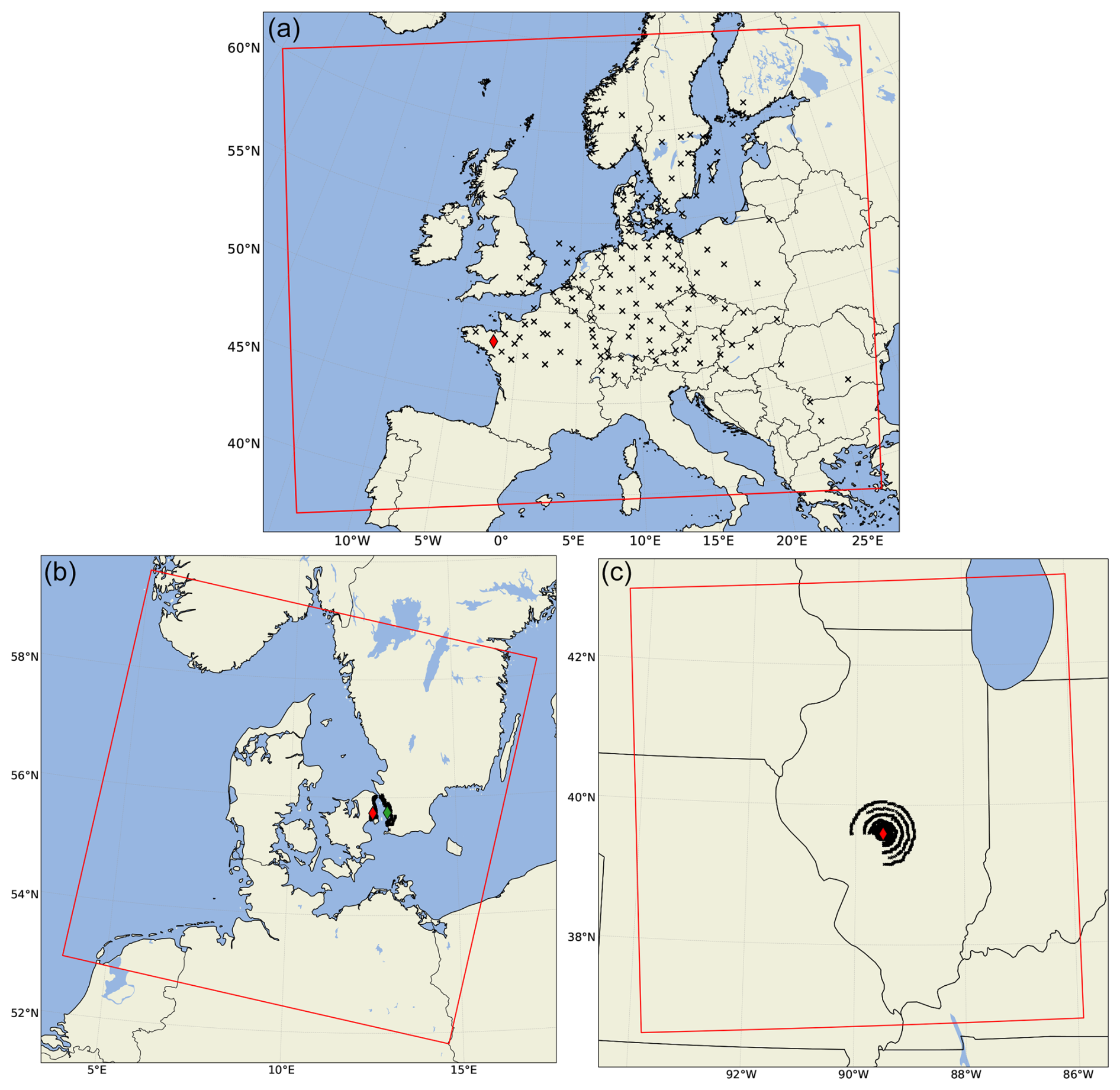
Figure 2 The three modeling domains used for the Harmonie simulations are indicated by the red squares in each plot. Panel (a) shows the domain used for ETEX. Panel (b) shows the domain used for the Øresund experiment. Panel (c) shows the domain used for the Kincaid experiment. In all three plots, the red (and green in the case of the Øresund experiment) diamond shows the release location, and the black crosses indicate the locations of sampling stations.

3.2 The Øresund experiment

The Øresund experiment consisted of nine non-buoyant sulfur hexafluoride (SF6) releases on different days from 16 May to 14 June 1984 (Mortensen and Gryning, 1989). Six releases were made from Barsebäck in Sweden (from 95 m above the ground), and three releases were made from the Gladsaxe mast in Denmark (from 115 m above the ground); release locations are shown in Fig. 2. In each of the releases, the release location was chosen based on the wind direction, such that the tracer was released near the upwind coast of Øresund and was sampled by a network of ground-based stations on the opposite coast. The sampling stations were typically configured in an arc near the coast and one or more arcs further inland. The dataset is thoroughly described by Mortensen and Gryning (1989) and is publicly available at https://doi.org/10.5281/zenodo.161966 (Mortensen and Gryning, 1987).

In this study, we use all the available ground-based measurements, but, when possible, measurements adjacent in time are averaged to provide average concentrations over longer time periods. This was done to reduce noise from the relatively short sampling periods (down to 15 min). For illustration, Fig. 3 shows the model predictions together with observations for a selected time during one of the Øresund releases. The example is not randomly selected but rather serves as a case demonstrating how the model improvements, in some scenarios, give a more realistic dispersion pattern.

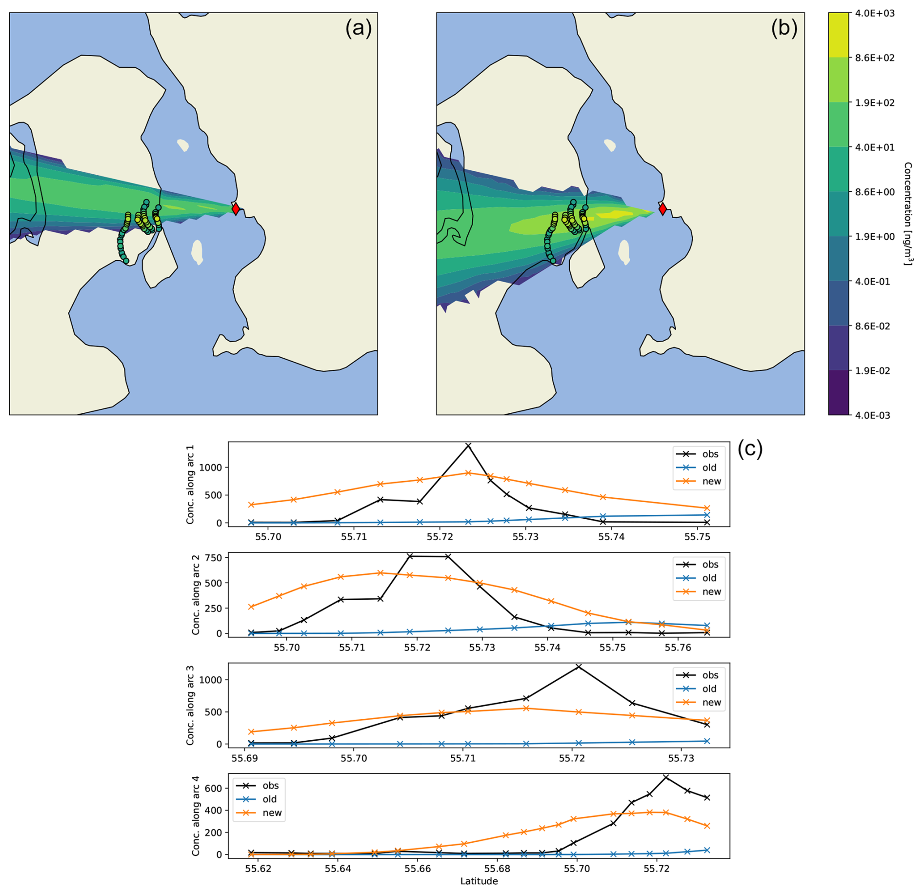
Figure 3 Examples of results are shown for a selected dispersion scenario for the Øresund experiment. The measurements and model results show average air concentrations during the interval 10:00 to 11:00 UTC, 6 June 1984. In the upper plots, the plumes show the model results of both the old (a) and new (b) models, while the dots show the measured values. In panel (c), observations are shown together with model predictions at the measurement locations. The arcs are numbered from 1 to 4, with 1 being the arc closest to the release location.

3.3 The Kincaid experiment

The Kincaid experiment consists of a series of SF6 releases spread out over three roughly 1-month-long periods in 1980 and 1981 (Bowne and Londergan, 1983). The gas was released from the 187 m high stack of the Kincaid power plant, located in Illinois, USA; see Fig. 2. In the surrounding area, primarily consisting of flat farmland with some lakes, air concentrations were sampled over 1 h periods by a network consisting of roughly 1500 potential sampling locations distributed in 12 arcs in varying distances from 0.5 up to 50 km downwind of the source. Not all samplers were active at all times, so the number of measurement locations varies. The SF6 tracer was released through the stack of the power plant, and the high gas temperatures often resulted in a substantial effective plume rise. The gas temperature and the exhaust velocity were measured and are available with relevant meteorological observations from a nearby weather mast (Bowne and Londergan, 1983).

The Kincaid data exist in different versions. One dataset is distributed as part of the Model Validation Kit (MVK) described by Olesen (2005), which is available at https://www.harmo.org/kit.php (last access: 12 March 2024). Another version of the Kincaid dataset was structured by John Irving and was distributed on his website, now maintained by the Harmo organization: https://www.harmo.org/jsirwin (last access: 12 March 2024).

As discussed by Olesen (2005), the concentration patterns were often irregular, with high and low values simultaneously occurring along the same arc. To provide a more robust foundation for model evaluation, arcwise maxima have been estimated along with a quality indicator ranging from 0 to 3 indicating how reliable each arcwise maximum is. The two abovementioned versions of the dataset differ slightly due to different algorithms used for assigning sampling stations to arcs and for assessing the quality of measurements; see https://www.harmo.org/jsirwin/KincaidHourlyDiscussion.html (last access: 12 March 2024). In this study, we use the version from John Irving, and both the entire set of SF6 measurements and the quality-controlled arcwise maximum values are used for the validation.

3.4 Experimental setup

For all three experiments, the simulations have been carried out using meteorological data from the limited-area NWP model Harmonie (Bengtsson et al., 2017). We use a horizontal grid resolution of approximately 2 km and a terrain-influenced hybrid vertical coordinate with 65 levels. The domains used for the simulations are shown in Fig. 2. For initial conditions and spatial boundary conditions, we use the ERA5 reanalysis (Hersbach et al., 2020, 2023).

Both versions of DERMA were then run for all three experiments. For the Kincaid experiment, the new model version was run with both of the plume rise algorithms described in Sect. 2.3. In all experiments, we use advection time steps of 3 min, and the sources have been discretized by releasing 50 puffs at every time step during the release period.

The resulting concentration fields have been interpolated in space using bilinear interpolation and integrated in time to obtain a list of modeled average concentrations corresponding to the set of observations. Denoting the observations x and the predictions y, we define the following statistical parameters used for model validation (cf. Draxler et al., 2001):

$$\begin{array}{}\text{(34)}& \begin{array}{rl}& \text{rmse}=\sqrt{{\displaystyle \frac{\mathrm{1}}{N}}\sum _i(y_i-x_i{)}^{\mathrm{2}}},\\ & \text{nmse}={\displaystyle \frac{\mathrm{1}}{N{\mathit{\mu }}_x{\mathit{\mu }}_y}}\sum _i(y_i-x_i{)}^{\mathrm{2}},\\ & r={\displaystyle \frac{(\mathit{x}-{\mathit{\mu }}_x)\cdot (\mathit{y}-{\mathit{\mu }}_y)}{{\mathit{\sigma }}_x{\mathit{\sigma }}_y}},\\ & b={\displaystyle \frac{\mathrm{1}}{N}}\sum _i{y}_i-x_i,\\ & \text{fb}={\displaystyle \frac{\mathrm{2}b}{{\mathit{\mu }}_x+{\mathit{\mu }}_y}},\\ & \text{fms}=\mathrm{100}{\displaystyle \frac{N(y>\mathrm{0})\cap N(x>\mathrm{0})}{N(y>\mathrm{0})\cup N(x>\mathrm{0})}},\\ & \text{foex}=\mathrm{100}\left({\displaystyle \frac{N_{(y_i>x_i)}}{N}}-{\displaystyle \frac{\mathrm{1}}{\mathrm{2}}}\right),\\ & {\text{fa}}_{\mathrm{2}}=\mathrm{100}\left({\displaystyle \frac{N_{(\mathrm{1}/\mathrm{2}<y_i/x_i<\mathrm{2})}}{N}}\right),\\ & {\text{fa}}_{\mathrm{5}}=\mathrm{100}\left({\displaystyle \frac{N_{(\mathrm{1}/\mathrm{5}<y_i/x_i<\mathrm{5})}}{N}}\right),\end{array}\end{array}$$

where μ and σ are the mean and standard deviation, rmse is the root-mean-square error, nmse is the normalized mean square error, r is the Pearson correlation coefficient, and b is the mean bias. Furthermore, fb is the fractional bias, which is a normalized measure of the mean bias ranging from −2 to 2; fms is the figure of merit in space, which is defined as the percentage of overlap between the measured and predicted areas; and foex is a measure of how many predictions are over-/underestimated, which is centered around zero and ranges from −50 % to 50 %. Finally, fa_α is the percentage of the predictions that are within a factor of $\mathrm{1}/\mathit{\alpha }$ to α from the observation. For the calculation of foex and fa_α, the 0–0 pairs are excluded. Due to the infinite nature of Gaussian distributions, a puff model technically always has non-zero predictions everywhere. For that reason, model predictions lower than the detection limit for each experiment are interpreted as non-detections.

3.5 Evaluation results

For all three experiments, the statistical parameters (Eq. 34) have been calculated and are shown in Tables 1–3. In Figs. 4–6, scatter plots of the model predictions as a function of the observed values are shown, along with quantile–quantile plots of predictions vs. observations. For the Kincaid experiment, the model is further evaluated using the arcwise maximum values with quality indicator 3 (best quality), shown in Table 4 and Fig. 7.

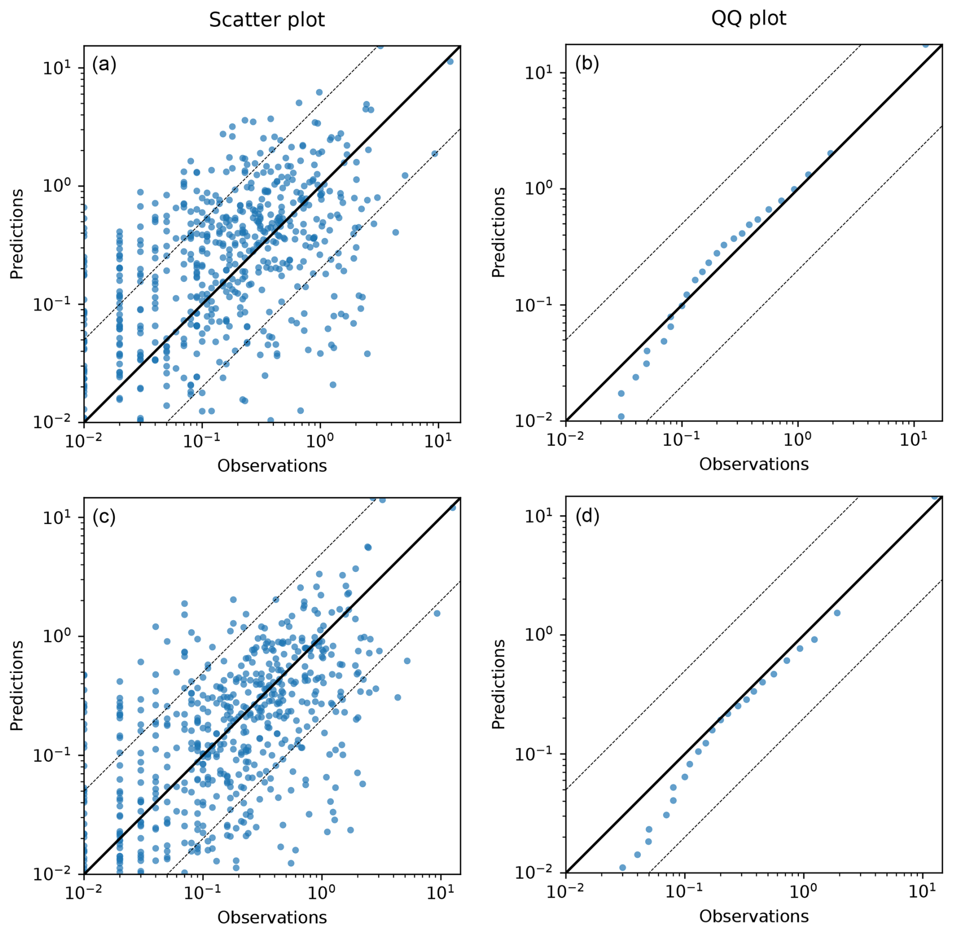
Figure 4 Results for the evaluation against ETEX. (a, c) Scatter plots of model predictions as a function of observations and (b, d) quantile–quantile plots. Concentrations are in ng m⁻³. Panels (a) and (b) are for the old version of DERMA, and panels (c) and (d) are for the new version. The solid black line indicates a perfect linear fit, and the dashed lines indicate deviations of a factor of 5 and $\mathrm{1}/\mathrm{5}$ away from the observation.

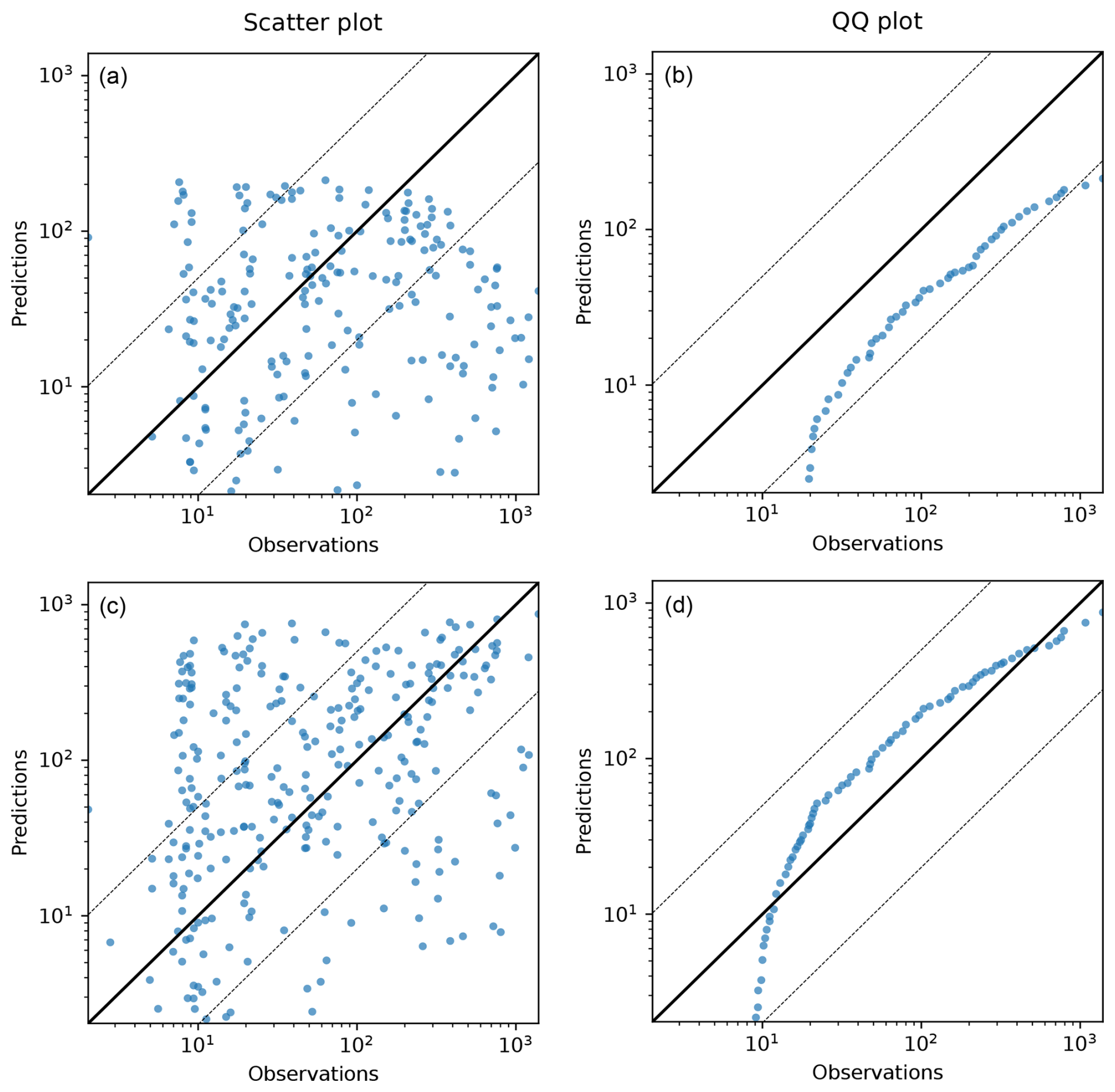
Figure 5 Results for the evaluation against the Øresund experiment. (a, c) Scatter plots of model predictions as a function of observations and (b, d) quantile–quantile plots. Concentrations are in ng m⁻³. Panels (a) and (b) are for the old version of DERMA, and panels (c) and (d) are for the new version. The solid black line indicates a perfect linear fit, and the dashed lines indicate deviations of a factor of 5 and $\mathrm{1}/\mathrm{5}$ away from the observation.

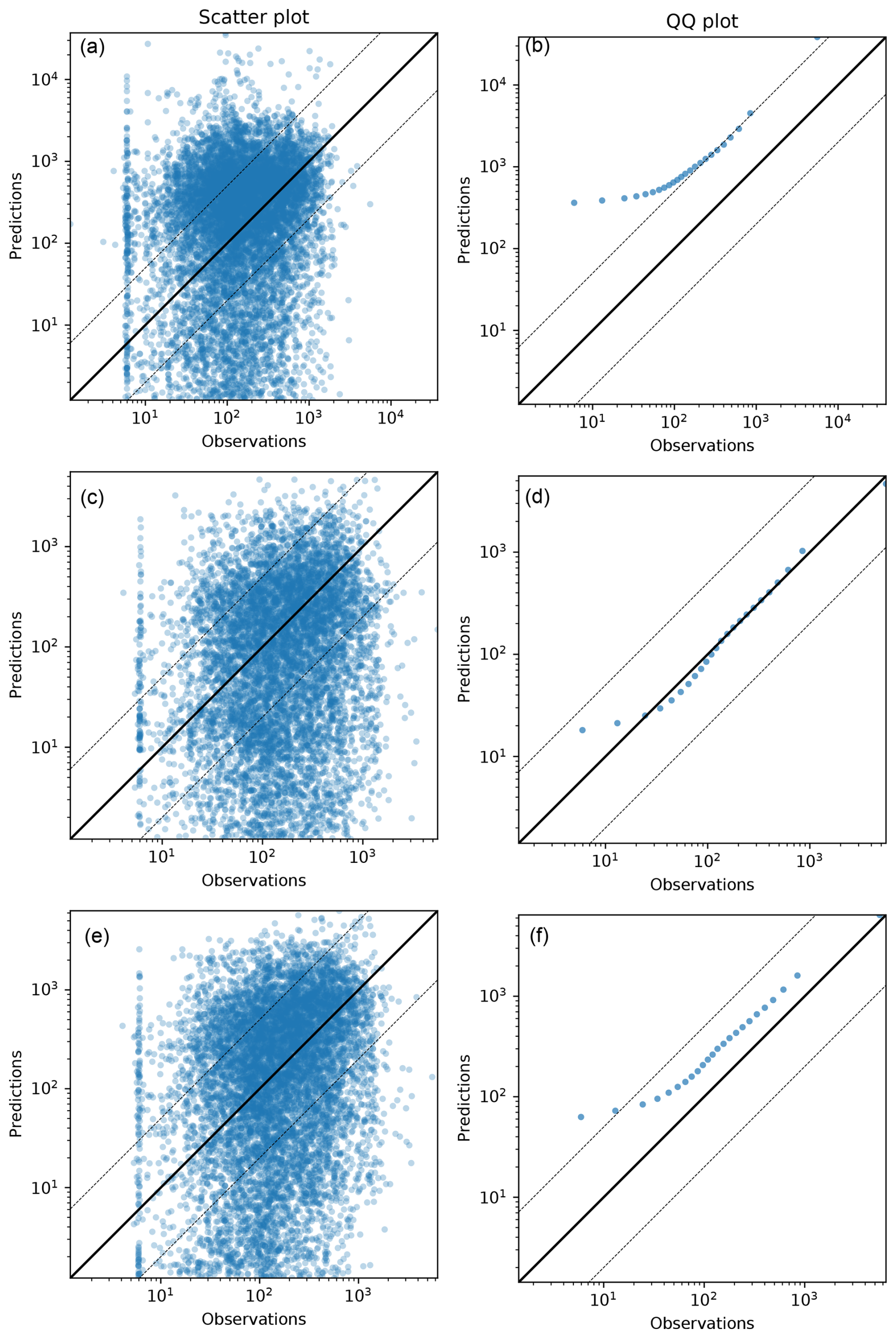
Figure 6 Results for the evaluation against the Kincaid experiment using alls available measurements. (a, c, e) Scatter plot of model predictions as a function of observations and (b, d, f) quantile–quantile plots. Concentrations are in ng m⁻³. Panels (a) and (b) are for the old version of DERMA, panels (c) and (d) are for the new version using the Briggs plume rise formula, and panels (e) and (f) are for the new version using the Concawe formula. The solid black line indicates a perfect linear fit, and the dashed lines indicate deviations of a factor of 5 and $\mathrm{1}/\mathrm{5}$ away from the observation.

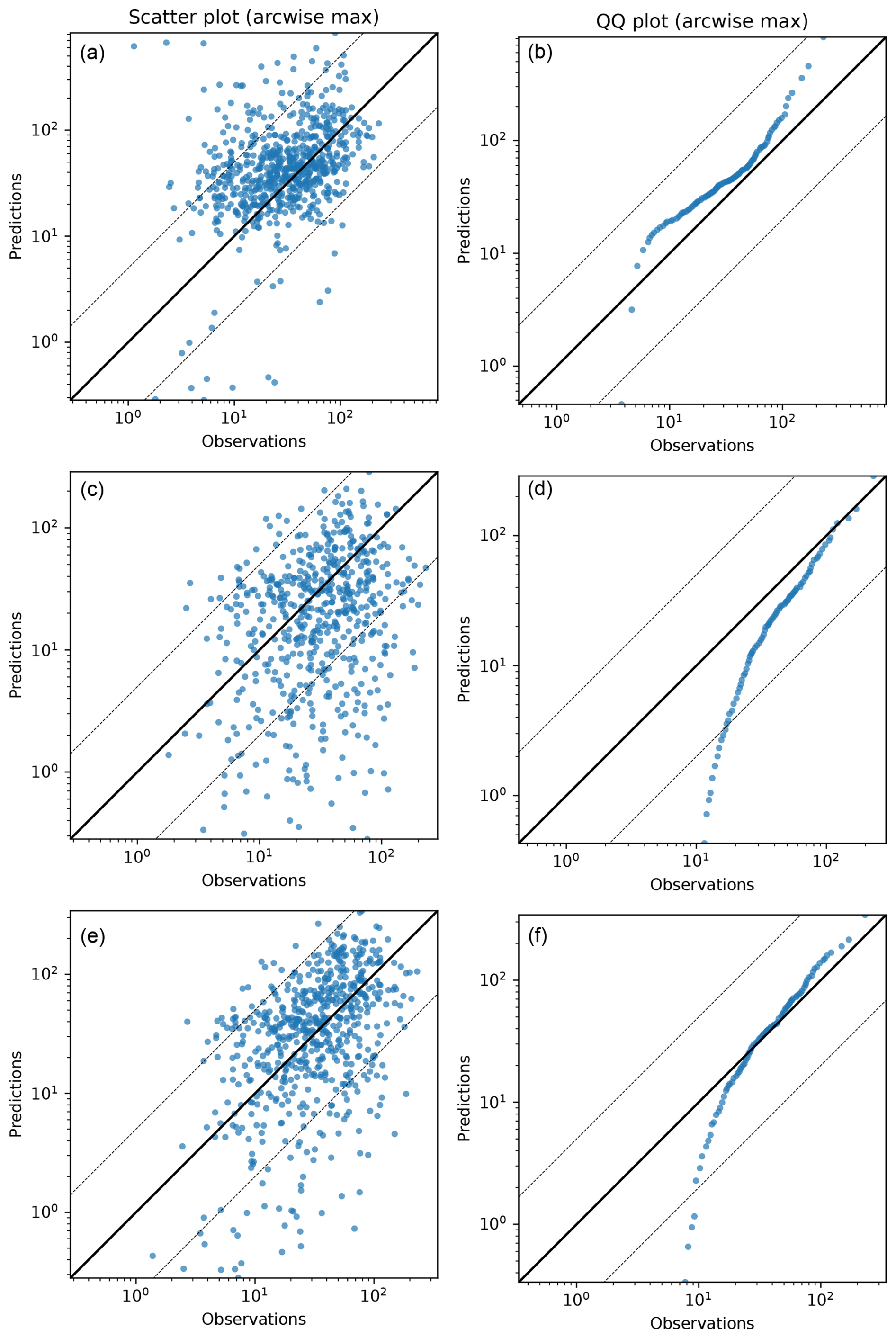
Figure 7 Results for the evaluation against the Kincaid experiment using arcwise maximum values with quality flag 3. (a, c, e) Scatter plots of model predictions as a function of observations and (b, d, f) quantile–quantile plot. Furthermore, concentrations have been divided by the mean release rate for the given release. Panels (a) and (b) are for the old version of DERMA, panels (c) and (d) are for the new version using the Briggs plume rise formula, and panels (e) and (f) are for the new version using the Concawe formula. The solid black line indicates a perfect linear fit, and the dashed lines indicate deviations of a factor of 5 and $\mathrm{1}/\mathrm{5}$ away from the observation.

Table 1 Statistical parameters, Eq. (34), calculated for ETEX.

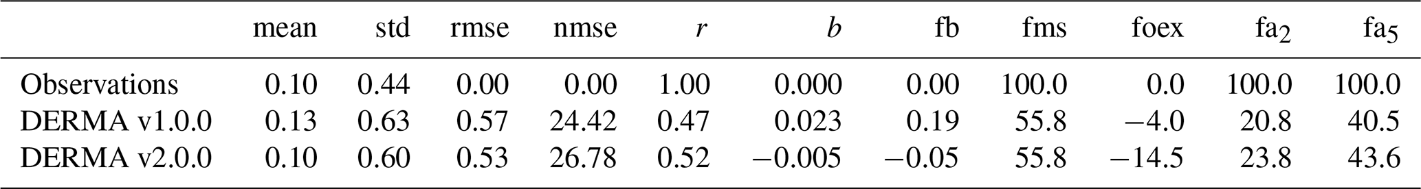
Table 2 Statistical parameters, Eq. (34), calculated for the Øresund experiment. When possible, longer time averages have been calculated to reduce the noise arising from the very short sampling periods; see Sect. 3.2 for further details.

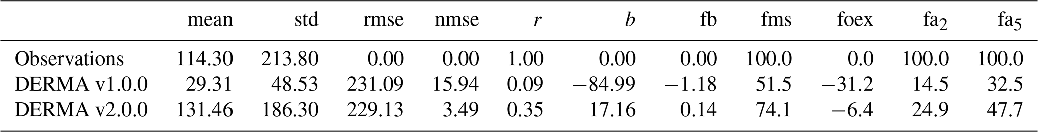
Table 3 Statistical parameters, Eq. (34), calculated for the Kincaid experiment using all available measurements.

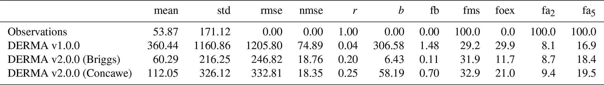
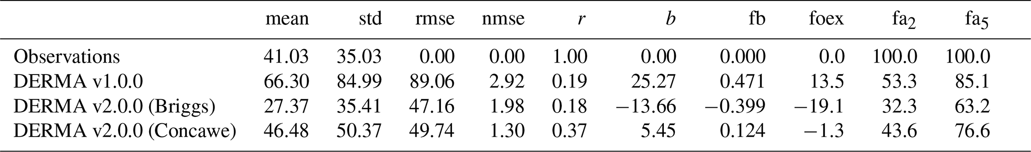
Table 4 Statistical parameters, Eq. (34), calculated for the Kincaid experiment using the arcwise maximum values with quality flag 3.

From Table 1, we see that the performances of the old and new models are quite similar for the ETEX experiment. The new model does show a slight improvement for the parameters r, b, fb, fa₂, and fa₅. For the other parameters, the old model performs slightly better, but the differences are very small in general, which is expected because the long-range formulation of the new hybrid approach is similar to that of the old version of DERMA, and there are few measurement stations close to the release point. From the scatter plots in Fig. 4, it does look like the new model has slightly less spread for higher values, while the quantile–quantile plots are very similar. Some statistical parameters, such as fa₂ and fa₅, may suggest a low level of agreement between the model predictions and observations. However, it is important to recognize that the Gaussian nature of the concentration distribution implies that even small shifts in plume position can produce large local discrepancies in surface concentration. Furthermore, these statistical parameters are consistent with those reported in the original model evaluation and thus fall within the expected range (Graziani et al., 1998).

The improved performance for long-range dispersion can likely be explained by the new stochastic transport scheme described in Sect. 2.1.2.

From Table 2, we see that the ground concentrations predicted by the old version of DERMA are systematically underestimated for the Øresund experiment. This is in accordance with the expectations due to the instantaneous vertical mixing throughout the PBL, which will cause lower concentrations near the source. In reality, the gas was released quite close to the ground, and we would therefore expect the ground concentrations to be high near the source. Essentially, the new model performs better across all statistical parameters, and the same is indicated by Fig. 5. Although none of the models correlate particularly well with the observations, the new model does predict high observed concentrations better, whereas the old model underestimates all the higher concentrations. The quantile–quantile plot also indicates that the new model is better on average, although it overestimates lower values and underestimates the highest observations.

For the Kincaid experiment, we firstly consider the results based on the full measurement dataset. Table 3 shows that the old model systematically overestimates the ground concentrations with a mean concentration of approximately 360 ng m⁻³, whereas the mean of the observations is roughly 54 ng m⁻³. This is again in accordance with the expectations: due to the plume rise, the effective release height is often quite high above the surface (therefore, the ground concentrations should be low near the source), whereas the old model mixes the tracer down to the surface from the start. The new version also has a positive bias, but the magnitude depends strongly on the plume rise algorithm used. The results obtained by using Briggs' formula give only a very small bias (average concentration of 60 ng m⁻³), while the results obtained by using the Concawe formula have an average of 112 ng m⁻³. The remaining statistics are quite similar for the two new models, and, for rmse, nmse, r, b, and fb, the performance is significantly better than for the old model, while, for the remaining statistics, there only seems to be a small improvement. Figure 6 also shows that there is a very large spread in the scatter plots for all three models. However, the quantile–quantile plots do suggest a significantly better representation of the concentration field with the new model, especially when using the Briggs plume rise scheme.

It should be noted that this comparison method is very sensitive to even small errors in the meteorological model data; since the spatial and temporal resolution of the measurements is so high, an error in, for example, the wind direction may result in large errors. Therefore, a more robust way of evaluating the model may be to compare model predictions with the arcwise maximum values. As described in Sect. 3.3, there were up to 12 arcs at distances of 0.5, 1, 2, 3, 5, 7, 10, 15, 20, 30, 40, and 50 km (not all arcs exist for all release periods). For every 1 h sampling period, the maximum value in each available arc is provided along with a quality indicator from 0 to 3. For the comparison, the predicted maximum concentration of each arc was estimated by firstly interpolating the concentration field to all sampling locations of that arc and then calculating the maximum value. The results in Table 4 and Fig. 7 are based only on maximum values with quality indicator 3.

In Table 4, the results are slightly more ambiguous than those from the previous comparisons. The new model using Briggs' formula performs slightly better than the old model for the parameters nmse, b, and fb, while the old model performs slightly better for foex, fa₂, and fa₅. However, the new model using the Concawe formula seems to stand out with better performance on all parameters except for fa₂ and fa₅, where the old model performs slightly better. Generally, all models perform much better on the arcwise maxima than when using the entire dataset, which confirms that this approach is less sensitive to errors in the predicted wind direction, for example. In Fig. 7, we also see that all three scatter plots have a much smaller spread than in Fig. 6.

Finally, it is relevant to note that there is quite a large difference in performance between the two new versions, which are identical except for the plume rise scheme used. This clearly indicates the importance of estimating the start height correctly in order to predict reliable ground concentrations near the source.

4 Summary and conclusions

This paper describes a new hybrid particle-puff formulation for dispersion modeling, making use of simple assumptions to separate turbulence into a stochastic particle part and a puff part, without the theoretical risk of double-counting turbulent effects. This formulation allows the use of a limited number of puffs and longer advection time steps compared to stochastic particle models. Furthermore, compared to the classical puff approach, it allows a more realistic description of turbulent diffusion for small puffs. For large puffs, on the other hand, the formulation allows puffs to be exposed to the vertical wind shear in the PBL without the need for puff splitting.

In addition, new parameterizations have been implemented in DERMA for turbulent wind fluctuation and Lagrangian timescales, for PBL height, and for plume rise. For the latter, both the Concawe formula and the Briggs formula have been implemented.

The model evaluation shows that implementation of the new hybrid approach improves the performance of DERMA for all three considered experiments. The evaluation method is not very robust, since the model predictions are very sensitive to meteorological errors. However, since our evaluation uses a large amount of measurement data sampled over many days during different times of the year, the overall trends in the results should give a good indication of the models' performances. Furthermore, the use of the arcwise maxima from the Kincaid experiment provides a completely different way of comparing model predictions with observations, which again indicates improved performance when using the new hybrid formulation.

Furthermore, a comparison of the two plume rise algorithms indicates how important it is to correctly estimate the initial plume height in order to predict the ground concentrations near the source. Unfortunately, there is no clear answer to which plume rise algorithm is best; in our evaluation, the Briggs formulas seem to give slightly better results when calculating statistics based on all data, while the Concawe formula performs better when compared to the arcwise maxima. However, the Concawe formula is somewhat more generally applicable because it only needs the released heat, whereas the Briggs formulas are specifically developed for gas being exhausted from a stack, and both gas temperature and exhaust velocity are necessary inputs.

In conclusion, the developed hybrid particle-puff formulation, in combination with the additional new implementations, has improved the performance of DERMA, especially for short-range dispersion modeling. Hence, these improvements could pave the way for new applications of DERMA in the future.