the Creative Commons Attribution 4.0 License.
the Creative Commons Attribution 4.0 License.
 | 10 Oct 2025
A trait-based model to describe plant community dynamics in managed grasslands (GrasslandTraitSim.jl v1.0.0)
Thibault Moulin
Oksana Buzhdygan
Britta Tietjen
Felix May
Temperate semi-natural grassland plant communities are expected to shift under global change, mainly due to land use and climate change. However, the interaction of different drivers on diversity and the influence of diversity on the provision of ecosystem services are not fully understood. To synthesize the knowledge of grassland dynamics and to be able to predict community shifts under different land-use and climate change scenarios, we developed the GrasslandTraitSim.jl model. In contrast to previously published grassland models, we link morphological plant traits to species-specific processes via transfer functions, thus avoiding a large number of species-specific parameters that are difficult to measure and calibrate. This allows any number of species to be simulated based on a list of commonly measured traits: specific leaf area, maximum height, leaf nitrogen per leaf mass, leaf biomass per plant biomass, above-ground biomass per plant biomass, root surface area per below-ground biomass, and arbuscular mycorrhizal colonization rate. For each species, the dynamics of the above- and below-ground biomass and its height are simulated with a daily time step. While the soil water content is simulated dynamically, the nutrient dynamics are kept simple, assuming that the nutrient availability depends on total soil nitrogen, yearly fertilization with nitrogen and the total plant biomass. We present a model description – which is complemented by online documentation with tutorials, flow charts, and interactive graphics – and calibrate and validate the model with two different datasets. We show that the model replicates the seasonal dynamics of productivity for experimental sites of the grass species Lolium perenne across Europe satisfactorily well. Furthermore, we demonstrate that the model can be used to simulate the productivity and functional composition of grassland sites with different numbers of mowing events and grazing intensity in three regions in Germany. Therefore, the GrasslandTraitSim.jl model is presented as a useful tool for predicting the plant biomass production and plant functional composition of temperate grasslands in response to management under climate change.
- Article
(11430 KB) - Full-text XML
- BibTeX
- EndNote


Permanent semi-natural grasslands cover 30.5 % of the agricultural area of the European Union (Eurostat, 2020), and many of them are known to support high levels of biodiversity (Petermann and Buzhdygan, 2021). At small spatial scales (< 100 m2), extensively managed grasslands have the highest recorded plant species richness per area in the world (Wilson et al., 2012). These plant-species-rich habitats can in turn support many other taxonomic groups, such as insects (European Environment Agency et al., 2013; Fartmann, 2024), which are adapted to open habitats. Moreover, 29 % of the European bird species are associated with grassland habitats (Nagy, 2009). In conclusion, temperate grasslands play an important role in supporting biodiversity in agricultural landscapes.
The key factor in maintaining the semi-natural grasslands in the temperate zone is management, as well as regular natural disturbances, such as low-intensity fires or avalanches, without which grasslands would become woodlands. This is because the abiotic conditions on most grassland sites favour tree growth by having the sufficient temperature, precipitation, soil moisture, and nutrients (Petermann and Buzhdygan, 2021). Mowing and/or grazing influence the plant species composition of grasslands and prevent the encroachment of woody species (Tälle et al., 2016). Therefore, grasslands and agriculture have been coevolving in Europe since the last glacial period (Hejcman et al., 2013; Pärtel et al., 2005). The intensity and type of land use influence the level of grassland biodiversity. Both intensification and abandonment can lead to a decline in grassland biodiversity (Gossner et al., 2016; Schils et al., 2020; Piseddu et al., 2021). Intensification, more specifically higher fertilization, more mowing events per year, and/or a higher livestock density, lead to a dominance of a few fast-growing plant species that are adapted to the high disturbance frequency by mowing and/or grazing. In particular, high fertilization results in the dominance of clonal species with wide runners and tall growth (Hejcman et al., 2007; Gough et al., 2012; Gross and Mittelbach, 2017). Abandonment, on the other hand, leads to the growth of woody species and a loss of specialists of open habitats (Hilpold et al., 2018). Management is therefore a key driver of plant community composition in the large majority of temperate grasslands.
Furthermore, climate change is expected to alter the plant community composition of grasslands, particularly during periods of heat waves and droughts, for example, by suppressing dominant species (Luo et al., 2025) and/or favouring plants with drought-avoidance strategies (Griffin‐Nolan et al., 2019; Schils et al., 2020). In addition, the diversity and composition of the plant community in grasslands affect the provision of ecosystem services, such as biomass production, resistance to climatic events, and pollination (Van Oijen et al., 2020; Buzhdygan et al., 2020). However, how different drivers and their interactions impact the community composition and how the composition relates to ecosystem service provision is poorly understood. In particular, the conditions under which a diverse plant community leads to higher biomass production remains a topic of debate (Adler et al., 2011; Chen et al., 2018; Dee et al., 2023). This highlights the need for a more comprehensive mechanistic understanding of the underlying processes. Simulation models can complement experimental and observational studies to predict the effects of management and climate change on grassland community dynamics and ecosystem service provision and can help to provide a better mechanistic understanding of processes. Current scientific knowledge is integrated into the models, and the models can be used to test hypotheses and to generate new knowledge (Clark et al., 2001; Jeltsch et al., 2008). Dynamic simulation models are therefore a useful tool for disentangling the effects of land use and climate on the plant community composition and the provision of ecosystem services by grasslands.
Historically, different research questions on grasslands, ranging from ecology to biogeochemistry, have led to the development of different grassland models by focusing on some parts of the grassland system while simplifying others (for an overview of representative models, see Table 1; for more detail, see Tables F1 and F2). In ecology, for example, questions about plant coexistence in grasslands have led to models with a strong focus on species interactions. In the biogeochemical community, questions were asked about the emission of greenhouse gases from grasslands, leading to the development of models with a focus on biogeochemical cycles in grasslands (Van Oijen et al., 2018). Ecological models are often simpler models and can be divided into difference or differential equation models and individual-based models. While individual-based models are characterized by a bottom-up approach by modelling the interactions of individuals, difference or differential equation models are characterized by a top-down approach by modelling the interactions of species, leading in both cases to the emergence of grassland community patterns. Examples of individual-based models are IBC-grass (May et al., 2009), originally developed to analyse the effects of grazing on plant communities; and GRASSMIND (Taubert et al., 2012), which can simulate the effects of climate change, mowing, fertilization, and irrigation on plant community dynamics. Examples of ecological differential equation models are DynaGraM (Moulin et al., 2021) and GraS (Siehoff et al., 2011), both of which can simulate the effect of mowing and grazing on the plant community. There are other more theoretical models that adopt the Lotka–Volterra differential equations for species competition to simulate grassland dynamics (Geijzendorffer et al., 2011; Fort, 2018; Pulungan et al., 2019; Chalmandrier et al., 2021). Competition between plant species is included in these models with interaction coefficients. The way that species or plant functional types are represented in all these models differ. The species in IBC-grass and GRASSMIND are described by morphological and physiological traits. GraS represents species mostly by species indicator values, and in DynaGraM species are represented by a combination of morphological and physiological traits and parameters derived from species indicator values. While IBC-grass, GraS, and the models using Lotka–Volterra-type equations focus strongly on ecological issues and are weak in representing biogeochemical cycles, GRASSMIND is coupled with a soil model, and DynaGraM has a basic representation of nutrient and water cycles included.
Chalmandrier et al. (2021)Moulin et al. (2021)Siehoff et al. (2011)Wirth et al. (2024)Confalonieri (2014)Piseddu et al. (2022)Taubert et al. (2012)Taubert et al. (2020)May et al. (2009)Table 1Overview of representative grassland models simulating several plant species or plant functional types. A more comprehensive overview, including models that simulate only one species, can be found in the appendix (Tables F1 and F2).
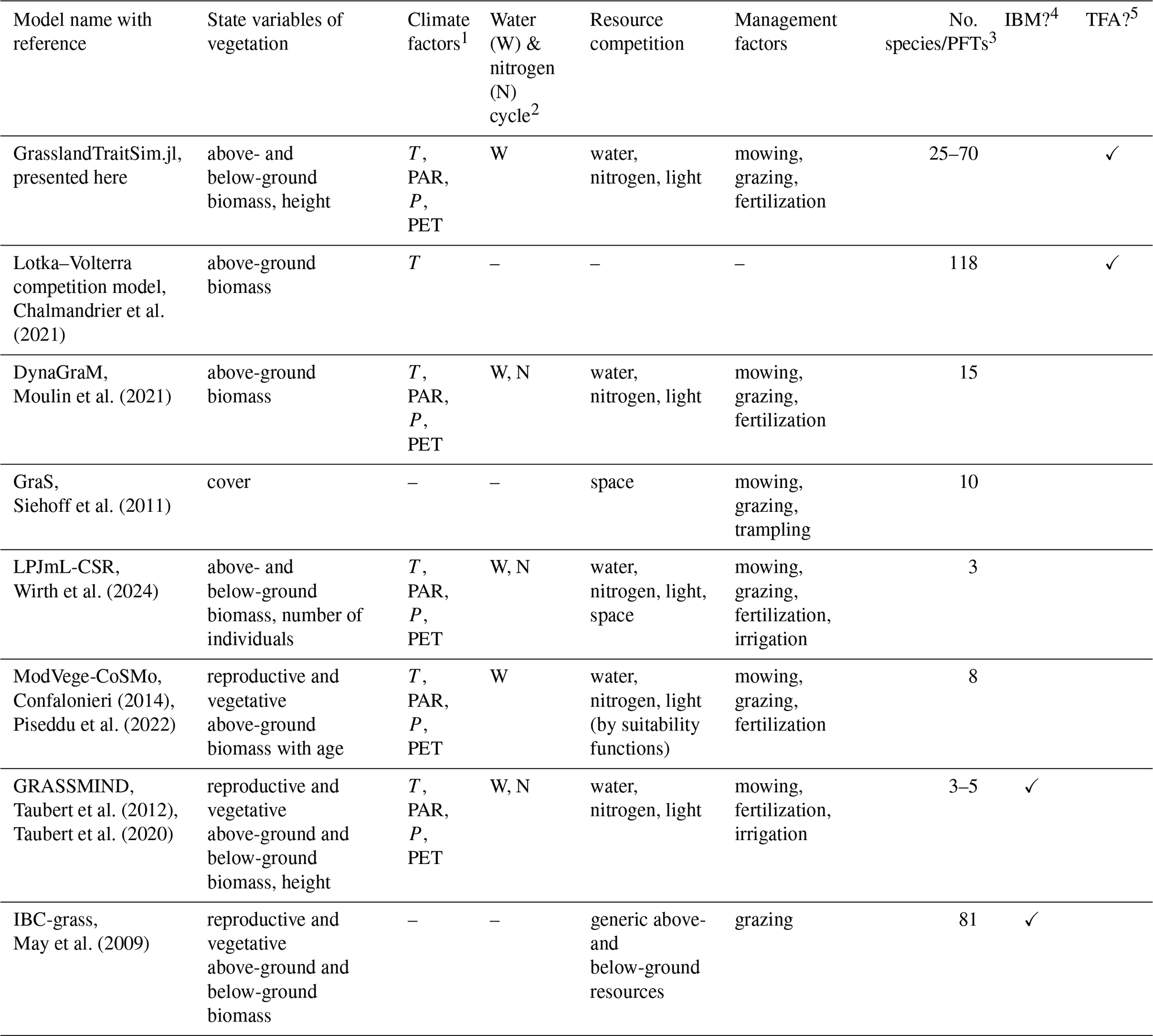
1 We have reviewed whether air temperature (T), photosynthetically active radiation (PAR), precipitation (P), and potential evapotranspiration (PET) are used in a model. Other external climate drivers, even if used in the specific model, are not shown in the table. 2 We evaluated whether the soil water and the soil nitrogen cycle are explicitly simulated in the models. 3 We reviewed the number of simulated species or plant functional types (PFTs), regardless of whether the species parameters were calibrated to data or whether the species were generated more theoretically. 4 We distinguish between individual-based models (IBMs), which directly simulate plant individuals; and population-based models, which simulate plant populations. 5 We distinguish between models in which parameters of transfer functions mapping morphological functional traits to species demographic rates are calibrated (TFA: “transfer function approach”) and models in which species demographic parameters are calibrated directly (Chalmandrier et al., 2021).
In contrast, models developed by the biogeochemical scientific community have a thorough representation of the nutrient, water, and carbon cycles in grasslands (Van Oijen et al., 2020). Examples include PaSim (Riedo et al., 1998), LPJmL (Rolinski et al., 2018), and CENTURY/DayCent (Parton, 1996; Parton et al., 1998). However, the representation of plant functional diversity in these models is limited. For example, in LPJmL, only two plant functional types (C3 and C4 grasses) are simulated in natural and managed grasslands (Rolinski et al., 2018). Recently, progress has been made to improve the representation of plant functional diversity by simulating C-, S-, and R-plant functional types in correspondence with the CSR model of plant strategies (Grime, 1977) in LPJmL (Wirth et al., 2024). Another approach to include a representation of plant functional diversity in a single-species grassland model is described by the CoSMo approach (Confalonieri, 2014). Before each time step, the relative abundance of several species is updated based on suitability functions of species to drivers. The relative abundance is used to calculate new community-weighted mean traits which are used as an input for the single-species grassland model for one time step. Thereby, the plant competition and the community growth dynamics are decoupled. An example is the coupling of the ModVege model with the CoSMo approach (Jouven et al., 2006; Piseddu et al., 2022). In summary, existing grassland models vary in their complexity in representing plant diversity and biogeochemical cycles and in how species are represented: by species indicator values, morphological traits, and/or physiological traits.
Modelling multi-species assemblages in grasslands has been identified as one of the key challenges in grassland modelling (Kipling et al., 2016). This is due to the fact that process-based grassland models require data on the physiological and demographic processes of species, such as measurements of growth rates of species under different radiation intensities. However, because demographic and physiological data are not readily available for many species, the number of species that can be modelled is limited (Jeltsch et al., 2008; Chalmandrier et al., 2021). To overcome the problem of missing demographic and physiological data, measurable morphological trait data can be used instead. Morphological trait data can be measured more easily and are available for many plant species, for example, from the plant trait database TRY (Kattge et al., 2020). For many morphological traits, it is known from experimental and observational studies how they affect species-specific processes (Funk et al., 2017). For example, a high specific leaf area is associated with high photosynthetic activity per leaf mass and a high senescence rate (Wright et al., 2004). So-called transfer functions can be built to map morphological parameters to physiological and demographic processes of species (“transfer function approach (TFA)”; see Table 1 and Chalmandrier et al., 2021). Parameters in the transfer function can control the strength of the link between morphological traits and physiological processes, for example, how strongly the specific leaf area correlates to the senescence rate of leaves. This has the technical advantage that the number of parameters for the model calibration does not increase with the species number. While this morphological trait-based approach enables broader species coverage and generality, it also comes with limitations. Morphological traits do not fully capture intra-specific genetic variation or phenotypic plasticity, both of which can be important for species' responses to environmental change. Additionally, environmental heterogeneity – such as soil texture, nutrient availability, and microclimate – may modulate the functional effects of traits in context-dependent ways.
Here, we use this transfer function approach of linking morphological traits to species-specific processes to develop the process-based model GrasslandTraitSim.jl. We extend the approach from Chalmandrier et al. (2021), which used a theoretical model with little or no representation of climate, management, and resource competition (see Table 1), to a model that can analyse the influence of management and climate on the productivity and plant functional composition of a grassland. The model is partly based on the DynaGraM model (Moulin et al., 2021), which in turn is based on LINGRA (Schapendonk et al., 1998) and ModVege (Jouven et al., 2006). Both ModVege and LINGRA simulate only one species or plant functional type (see Table F1). With DynaGraM, it is possible to study the influence of climate and management on the productivity and plant functional composition, and DynaGraM can simulate several species. However, DynaGraM does not rely solely on morphological species-specific parameters but uses instead a combination of morphological, demographic, and indicator values (see Table F2). This hinders the use of the transfer function approach of linking morphological traits to species' demographic rates and has the disadvantage of the species-specific demographic parameters not being available for many plant species. We decided to design a population-based model to not have the computational cost of calibrating an individual-based model. Moreover, we decided to keep the plant competition directly in the growth dynamics, as in the DynaGraM model, and not update the relative abundance of the species based on suitability functions, as with the CoSMo approach (Confalonieri, 2014). Our model is of intermediate complexity compared to the above-mentioned models in terms of the number of equations, which is reflected in the number of simulated state variables and the number of parameters (species-specific and global non-species-specific parameters, see Tables 1, F1, and F2). Consequently, our GrasslandTraitSim.jl model addresses a gap in existing grassland simulation models by simulating multi-species assemblages and predicting the functional composition of plant communities in response to management practices and climate change. As plant functional composition influences biomass supply in the model, cascading effects from management and climate through plant functional composition to biomass supply can be analysed. We will present a comprehensive model description and calibration and validation using two different datasets of managed grasslands in Europe.
The GrasslandTraitSim.jl model is designed to simulate the dynamics of grassland communities under different management scenarios and soil and climatic conditions. The state variables of many plant species (denoted by the subscript s) are simulated with daily time steps (indicated by the t subscript): above-ground dry biomass BA,ts [kg ha−1], below-ground dry biomass BB,ts [kg ha−1], and height Hts [m]. The sum of the above-ground and below-ground dry biomass equals the total dry biomass Bts [kg ha−1]. Additionally, the state variable soil water content in the rooting zone Wt [mm] is simulated (Fig. 1). Changes in the state variables from one day to the next are described by a set of difference equations (for details, see Table ). The morphological functional traits of all plant species are fixed (time-invariant inputs, for example, the maximum plant height) and are linked by model parameters to the species' demographic processes (Fig. 2). As a result of the differences in the demographic rates of all species, the performance of individual plant species differs (biomass increase or decrease under particular conditions), leading to the emergence of plant community dynamics. While reading the model description, we encourage the reader to have a look at the online documentation, which contains many interactive graphics and flow charts that make the model description more accessible (see the data availability statement).
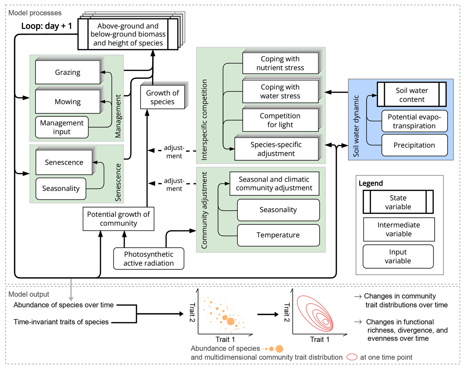
Figure 1Structure of the GrasslandTraitSim.jl model. Boxes represent state, intermediate, and input variables (forcing functions), and arrows indicate the influence of one variable on another. We use the term “intermediate variables” to describe variables that are neither inputs nor state variables but are important intermediate results in the calculation of the change in state variables. While the green areas show calculations that influence the change in above- and below-ground biomass and height, the blue area shows the calculation of the change in soil water content in the rooting zone. The arrows originating from the biomass and height of the species indicate that both the biomass and height play a role in the processes outlined in the green and blue areas. However, for simplicity, they do not indicate the exact position within the areas. Species-specific variables are represented by a series of offset boxes positioned behind one another, indicating the presence of multiple species within the model. We show how the distribution of community traits can be calculated from the model output; other model outputs include the state variables and the grazed and mown biomass, which can be summarized at the community level.
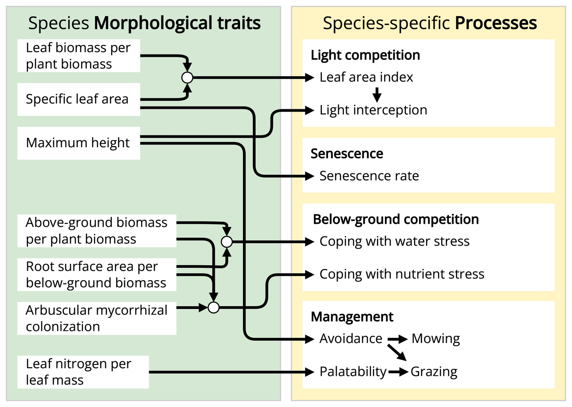
Figure 2The GrasslandTraitSim.jl model links morphological plant functional traits to processes. Arrows indicate which process or variable is influenced by each plant functional trait. Each plant functional trait can have species-specific values, allowing for species-specific responses in many of the model's processes.
The required model inputs are the plant functional traits of each species, soil properties, daily climatic data, and daily management data (e.g. timing and intensity of grazing, Table F3). The model has in total 54 global parameters (for details, see Table F4) that are not site, time, or species dependent. Outputs include the state variables and the grazed and mown biomass. The simulated abundance distribution can be summarized using taxonomic diversity indices (e.g. Simpson diversity) and plant functional diversity indices (e.g. functional dispersion and functional evenness), as well as community-weighted means and variances of each trait. All of these outputs can be calculated for each day. The model is not spatially explicit and does not account for spatial heterogeneity. As the assumption of spatial homogeneity is met only approximately for smaller spatial dimensions, we suggest using the model for areas between 1 m2 and 1 ha.
The model procedure is divided into an initialization and a simulation part. During the initialization, the state variables (height, above-ground and below-ground biomass of species, and soil water content) are set to user-supplied initial values. During the simulation, a loop is run over each day. For each day, very low or negative values () of the height Hts and biomass state variables (Bts, BA,ts, and BB,ts) are set to zero to avoid numerical problems. We have deliberately kept the threshold at a low level because the plant species should be able to recover, even from a very low biomass level. After that, the main part of the model is executed with the calculation of growth (Sect. 2.1–2.1.7, Eqs. 5–33), senescence (Sect. 2.1.8, Eqs. 34–35), biomass removal by management (Sect. 2.1.9, Eqs. 36–42), height dynamics (Sect. 2.2, Eq. 43), and soil water dynamics (Sect. 2.3, Eqs. 44–52).
2.1 Biomass dynamics
The change in the total biomass B from day t to t+1 of species s [kg ha−1] is calculated based on the actual growth Gact,ts [kg ha−1] (Eq. 5) and the losses by senescence Sts [kg ha−1] (Eq. 34) and management Mts [kg ha−1] (Eq. 36):
The change in the total biomass Bts is divided into the change in above-ground BA,ts [kg ha−1] and below-ground biomass Bts [kg ha−1]. We assume that plants aim to achieve a similar level of above-ground biomass per total biomass, similar to the time-invariant trait above-ground biomass per total biomass abps [−]. We therefore calculate Ats [−] as the ratio between the actual biomass ratio and the trait abps:
Ats is less than 1 if the above-ground biomass per total biomass is less than expected by the trait abps, for example, after a mowing event. This variable can be used to allocate biomass changes by growth and senescence to above-ground and below-ground biomass. Biomass loss by mowing and grazing affects only the above-ground biomass:
This formulation allows for the rapid regrowth of the above-ground biomass after a grazing period or a mowing event, as little of the growth is allocated to below-ground biomass and most is allocated to above-ground biomass.
The actual growth is derived from the community potential growth Gpot,t [kg ha−1] (Eq. 6) and the multiplicative effect of five growth adjustment factors:
where LIGts [−] is the species-specific competition for light (Eq. 12), NUTts [−] is the species-specific competition for nutrients (Eq. 15), WATts [−] is the species-specific competition for soil water (Sect. 2.1.5), ROOTts [−] is the species-specific cost for maintaining roots and mycorrhiza (Eq. 26), and ENVt [−] is the non-species-specific adjustment based on environmental and seasonal factors (Eq. 29).
2.1.1 Community potential growth
The model follows the concept of the light-use efficiency (Monteith, 1972) that describes how much dry matter the plants can build based on the solar radiation. This concept was widely adopted in grassland modelling studies (Schapendonk et al., 1998; Jouven et al., 2006; Moulin et al., 2021; for a review, see Pei et al., 2022). The community potential growth Gpot,t is described by
with the photosynthetically active radiation PARt [MJ ha−1], maximal radiation use efficiency γRUEmax [kg MJ−1], and the fraction of PARt that is intercepted by the plants FPARt [−].
The modelled fraction of radiation intercepted by the plants is determined by the number of leaves and the height of the community. A saturation function is used to describe the relationship between leaf area per ground area (leaf area index) and light interception. We argue that light interception is less effective when all plants are rather short, because the leaves are more densely packed. Individual plants avoid shading by growing taller (Heger, 2016). Therefore, we include the height of the community in the light interception calculation, also to prevent a community with short plants from building up a very high biomass. More technically, we use the Beer–Lambert equation to model the non-linear response of the fraction of light-intercepted FPARt to the total leaf area index LAItot,t (Monsi, 1953; Monsi and Saeki, 2005). This relationship is governed by the light extinction coefficient γRUE,k [−], which determines how quickly the fraction of absorbed radiation approaches 1 as the leaf area index increases. The reduction in radiation use efficiency because of densely packed leaves is a function of the community-weighted mean height and is influenced by the parameter [−], which specifies the growth reduction at . The 0.2 m has been arbitrarily set, and the parameter αRUE,cwmH is inversely calibrated. If Hcwm,t is greater than 0.2 m, less self-shading will occur because the leaves are less densely packed, and therefore the growth reduction is less than αRUE,cwmH:
with the community-weighted mean height calculated by weighting the height Hts [m] of each species by its share of above-ground biomass BA,ts of the total above-ground biomass BtotA,t [kg ha−1]:
The total leaf area index LAItot,t is the sum of the species-specific leaf area indices LAIts:
where LAIts is defined as
with above-ground biomass BA,ts [kg ha−1], specific leaf area slas [m2 g−1], and leaf biomass per above-ground biomass lbps [−]. As BA,ts and slas must be converted to the same unit, Eq. (10) is multiplied by 0.1.
2.1.2 Species-specific light competition
In our model, the proportion of total community biomass growth attributed to each species is determined by its leaf area index and height. Plant species with a high leaf area index per unit of biomass transfer more above-ground biomass to their leaves and have thinner leaves. These species can build a greater leaf area, allowing them to use the photosynthetically active radiation more efficiently per unit of biomass. Moreover, plant species that are taller than other species receive greater light exposure and are less affected by shading from other plant species (Falster and Westoby, 2003; Anten and Hirose, 1999). A situation in which taller species exploit relatively more light for growth than their biomass proportions is described by the term “size-asymmetric competition” (Weiner, 1990; Schwinning and Weiner, 1998). Some plant species devote more resources to supporting tissue (such as stems), resulting in taller plants that are less affected by shading. Other species invest more in leaves, resulting in a higher leaf area per unit of biomass. It is not possible to maximize both characteristics simultaneously, demonstrating a common trade-off in plant strategies (Westoby et al., 2002). Which strategy dominates depends on abiotic factors and biotic interactions. For example, fertilization can cause a shift in the grassland plant community towards taller clonal species (Gough et al., 2012; Dickson et al., 2014).
The proportion of light intercepted by each species out of the total light intercepted is derived by dividing the sward into vertical height layers of constant width, by default 0.05 m, to account for shading (similar to Taubert et al., 2012). We want to calculate how much light is intercepted in each height layer l INTt,l [−]. Therefore, we need to calculate how much light is intercepted in the layers above and the interception in layer l. We assume that the biomass, and therefore also the leaf area index, is uniformly distributed over the height of the plant. Thus, we can calculate the leaf area index of each species in each height layer LAIts,l [−] and the total leaf area index of all species in each layer LAI [−]. For each layer, we can calculate the total leaf area index above the layer up to the maximum height layer L. The maximum height layer can be reached by the tallest plants with the highest maxheight [m]. The reduction in incoming light based on the total leaf area index of the layers above and the interception of layer l is used to calculate the proportion of light intercepted in layer l INTt,l:
The proportion of light intercepted in the layer can be used to obtain the proportion of light intercepted for each species in each layer by multiplying INTt,l by the leaf area index proportion of the layer. The sum of all species-specific light interception proportions across all layers can be used to calculate the light competition factor LIGts [−]:
We divide the term by the total interception of all layers (compare Eq. 7) to ensure that the sum of all species-specific light competition factors is equal to 1.
2.1.3 General form of the growth reducer for nutrient and water stress
We use the same equations with different parameters to relate the plant-available nutrients and plant-available soil water to the growth reducers of nutrient and water stress. Therefore, we show here the general form of the equations (see Fig. 3) to avoid repetition and to define the specific variables and parameters used in the next two sections on nutrient and water stress. The derivation of the equations is shown in more detail in Appendix A. We use a logistic function to relate the resource density Rt (general symbol for the plant-available nutrients Np,ts and the plant-available water Wp,t) to the growth reducer REDts (general symbol for the growth reducers for nutrient stress NUTamc,ts and NUTrsa,ts and water stress WATts). The growth reducer REDts lies between zero (no growth possible) and 1 (no growth reduction at all). While the inflection points of the logistic function (general symbol for , , and ) are species specific depending on the trait values traitts (general symbol for the root surface area per total biomass TRSAts and the arbuscular mycorrhizal colonization rate per total biomass TAMCts), the slope βRED (general symbol for βNUT,rsa, βNUT,amc, and βWAT,rsa) is not species specific. We assume that if the plant has a trait value equal to the parameter ϕtrait (general symbol for ϕTRSA and ϕTAMC), then the growth reduction at 0.5 resource density is αRED,05 (general symbol for , , and ). If the parameter ϕtrait is set to the mean trait of a community, then the parameter αRED,05 can be interpreted as the mean response at half the maximum resource density. How much the inflection points deviate from this mean response can be controlled by the parameter δRED (general symbol for δNUT,rsa, δNUT,amc, and δWAT,rsa). If δRED is zero, there is no difference in the growth reduction between the species. If δRED is greater than zero, species with higher trait values are less affected by nutrient or water stress:
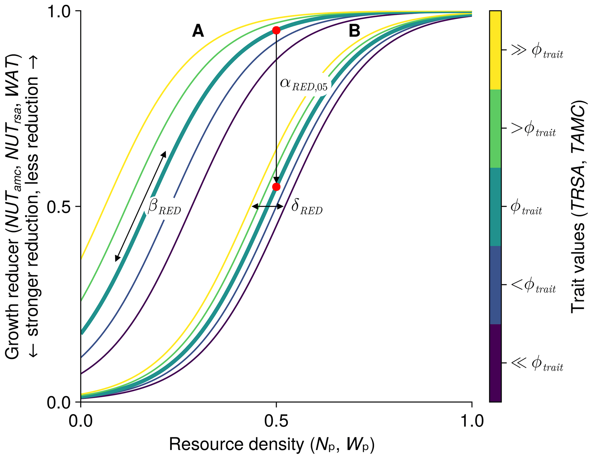
Figure 3General form of growth reducer as a function of resource density (plant-available nutrients and soil water). The function is governed by the four parameters βRED (slope of the logistic function), ϕtrait (usually the mean trait value), αRED,05 (growth reduction at half the resource density for species with a trait value of ϕtrait, marked by a red dot), and δRED (controls how much the species-specific inflection points differ from the inflection point of a species with a value of ϕtrait). We show two different curves for different parameter values: A with and δRED=0.25; B with and δRED=0.1. In both cases we used βR=9; ϕtrait=20; and the trait values 16, 18, 20, 22, and 24 (from dark purple to yellow). We include dynamic versions with sliders for the parameters for the three growth reducers NUTamc,ts, NUTrsa,ts, and WATts in the Supplement (see data accessibility statement).
2.1.4 Species-specific nutrient stress
Plant growth may be reduced when soil nutrient availability is low and plants are inefficient at taking up nutrients. We assume that the arbuscular mycorrhizal colonization rate (Marschner and Dell, 1994; George et al., 1995; Van Der Heijden et al., 2015) and the root surface area per total biomass (Barber and Silberbush, 1984) represent strategies in the nutrient uptake. High values of these traits lead to increased nutrient uptake rates and, consequently, reduced nutrient stress. Here, we only consider nutrient deficit as nutrient stress. The growth reducer NUTts [−] is composed of the maximum out of two nutrient stress factors that are linked to the arbuscular mycorrhizal colonization rate Namc,ts [−] and the root surface area per total biomass Nrsa,ts [−]:
The maximum of the two nutrient stress factors is used because, for simplicity, we assume that plants can invest either in a high root surface area per total biomass or in a high rate of arbuscular mycorrhizal colonization. Plants with a higher root surface area per total biomass follow the strategy of taking up nutrients themselves, while plants with high arbuscular mycorrhizal colonization rates follow the strategy of outsourcing nutrient uptake to arbuscular mycorrhizal fungi in the context of the root collaboration gradient (Bergmann et al., 2020). Since growth is reduced by how well plants follow their best strategy, the maximum of the two reduction factors is used to calculate the reduction in growth due to soil nutrients.
For the calculation of the growth reducers for nutrient stress based on the arbuscular mycorrhizal colonization rate NUTamc,ts [−], we use the parameters ϕTAMC [−], βNUT,amc [−], [−], δNUT,amc [−]; and for nutrients stress based on the root surface area per total biomass NUTrsa,ts [−], we use ϕTRSA [m2 g−1], βNUT,rsa [−], [−], and δNUT,rsa [g m−2]. Moreover, we still need the trait values and the plant-available nutrients (to replace traits and Rt in Eqs. 13–14).
For the traits that influence the nutrient growth reducer, we consider that plants with high below-ground biomass per total biomass are less affected by low nutrient levels because they have relatively more root tissue to supply nutrients to the above-ground biomass. It has been shown that the root-to-shoot ratio increases in many plants under nitrogen-poor conditions (Jiang et al., 2016; Meurer et al., 2019; Lopez et al., 2023). Therefore, we calculate the root surface area per total biomass TRSAts [m2 g−1] and the arbuscular mycorrhizal colonization rate per total biomass TAMCts [−] from the fixed-traits root surface area per below-ground biomass rsas and arbuscular mycorrhizal colonization rate per root tissue amcs with the dynamic proportion of the below-ground biomass BB,ts per total biomass Bts:
where the below-ground biomass is cancelled out. TAMCts and TRSAts are used to replace the trait in Eq. (13) for the calculation of NUTamc,ts and NUTrsa,ts.
The nutrients available to plants depends on the total soil nitrogen of site N [gN kg−1], the fertilization with nitrogen F [kgN ha yr−1], and the density effect (which accounts for stronger competition for nutrients if many plant species have a high biomass). The fertilization rate can vary between years and is the sum of organic and inorganic fertilization with nitrogen per year. More technically, the empirical parameters ωNUT,N [gN−1 kg] and ωNUT,F [] control how strongly the variables total soil nitrogen and fertilization rate, respectively, contribute to the value of the nutrient index (). The nutrient index is multiplied by the nutrient adjustment factor NUTadj,ts [−], which accounts for the biomass density, to get the plant-available nutrients Np,ts [−]:
The plant-available nutrients Np,ts are used in Eq. (14) for the resource Rt to calculate the growth reducers of NUTamc,ts and NUTrsa,ts. Np,ts can be greater than 1 if the total biomass is low; then growth is not reduced (see Eq. 14). In contrast to the plant-available water (Eq. 25), the plant-available nutrients are species specific.
Plants are most strongly affected by below-ground competition if conspecifics and plants with similar traits have a high biomass and share the below-ground resources. This is summarized with the nutrient adjustment factor NUTadj,ts [−], which takes into account the biomass and the trait similarity between all species:
with the trait similarity TSs,i [−] between species s and i, the biomass of species i Bti [kg ha−1], and the parameters αNUT,TSB [kg ha−1] and αNUT,maxadj [−]. A high nutrient adjustment factor NUTadj,ts is favourable for a species because the factor is multiplied by the site nutrients (Eq. 18), which means that the species has to share the resources with fewer competitors. More specifically, a high NUTadj,ts of a species indicates that either the total biomass is low or that the plant has traits that are very different from the traits of the abundant plant species. The parameter αNUT,TSB is a reference value for the sum of the product of trait similarity and the biomass of all species. If the sum of the product of trait similarity and biomass of all species is equal to αNUT,TSB, the nutrient adjustment factor is 1. The parameter αNUT,maxadj (≥1) controls the maximum of the nutrient adjustment factor. The parameter can be greater than 1 to allow the plant-available nutrients to be increased when the total biomass is low.
The trait similarity is derived by calculating the dissimilarity of the root surface area per above-ground biomass rsas [m2 g−1] and the arbuscular mycorrhizal colonization rate amcs [−] between all species and converting it to a similarity index. These two traits are chosen to calculate the trait dissimilarity index, because both traits encompass unique plant strategies for the acquisition of nutrients and water (Bergmann et al., 2020). The trait dissimilarity TDs,i [−] between species s and species i is calculated by the Euclidean distance between the normalized traits of the species:
This gives the dissimilarity matrix TD [−], which is transformed and scaled by the parameter βNUT,TS [−] to a trait similarity matrix TS [−]:
If βNUT,TS is zero, the trait similarity has no influence in the calculation of the nutrient adjustment factor in Eq. (19).
2.1.5 Species-specific water stress
Plant growth may be restricted under conditions of low soil-water content, particularly if the plants exhibit a limited water-uptake efficiency. We consider the root surface area per total biomass TRSAts [m2 g−1] (see Eq. 17) as the trait that influences how strong plants are exposed to the water stress at a certain soil water level. Here, we only consider too little water leading to water stress conditions, not too much water, as the primary goal of our model is not to model systems with regular flooding or waterlogging. We use the same equations for the water stress reducer WATts [−] as for the nutrient reducer (see Eqs. 13–14) with the parameters ϕTRSA [m2 g−1], βWAT,rsa [−], [−], and δWAT,rsa [g m−2]. The same explanation for the parameters applies as for the nutrient reducer.
The plant-available water is the rescaled soil water content (to replace R in Eq. 14): the soil water content Wt [mm] is scaled by the water-holding capacity WHC [mm] (Eq. 51) and the permanent wilting point PWP [mm] (Eq. 52) to scale water availability between zero (soil water content at or below the permanent wilting point) and 1 (soil water content at or above the water-holding capacity). The plant-available water Wp,t [−] is defined as
This formulation of plant-available water does not take into account some short-term temporal dynamics. For example, after a rainfall event, plants are often not water stressed at all, even if the soil water content is not replenished to the water-holding capacity.
2.1.6 Species-specific maintenance costs for roots and mycorrhizae
Maintaining a fine-root structure and symbiosis with mycorrhizal fungi costs energy. These costs include respiration (Caldwell, 1979), the production of metabolites for nutrient uptake (Canarini et al., 2019), and the supply of photosynthetic products to the mycorrhizal fungi (Konvalinková et al., 2017). Similarly to Taubert et al. (2012), who consider the costs of maintaining a symbiosis with nitrogen-fixing rhizobia, we include a cost term for root surface area per total biomass ROOTrsa,ts [−] and the mycorrhizal colonization rate per total biomass ROOTamc,ts [−]. This means that part of the potential growth cannot be used to produce new biomass:
where ROOTts [−] is the root investment factor that lowers the actual growth in (Eq. 5):
where TRSAts is the root surface area per total biomass [m2 g−1] (see Eq. 17), and TAMCts is the arbuscular mycorrhizal colonization rate per total biomass [−] (see Eq. 16). Therefore, the cost of maintaining fine roots and mycorrhizae does change with time, depending on the ratio between above-ground and below-ground biomass.
The parameters κROOT,rsa [−] and κROOT,amc [−] define the maximum possible growth reduction from zero to 1, where zero means no growth reduction at all. The parameters ϕTRSA [m2 g−1] and ϕTAMC [−] define the trait values of TRSAts and TAMCts at which the growth reducer is half in between 1 (no growth reduction) and the maximal growth reduction that is defined by κROOT,rsa and κROOT,amc. Note that the same values for ϕTRSA and ϕTAMC are also used for water- and nutrient stress reducers.
2.1.7 Community environmental and seasonal factors
The growth is adjusted for environmental and seasonal factors ENVt that apply in the same way to all species (Eq. 5). For simplicity, we do not consider the effect of species-specific plant traits on the following functions:
with the radiation RADt [−] (Eq. 30), temperature TEMPt [−] (Eq. 31), and seasonal SEAt [−] (Eq. 32) the growth adjustment factors.
Plant growth increases with photosynthetically active radiation (as formulated in Eq. 6), but excess radiation can lead to oxidative damage and photoinhibition (Long et al., 1994). We have therefore included the equation and parametrization from Schapendonk et al. (1998) that reduces the growth due to excess radiation. The radiation adjustment factor RADt [−] is calculated as follows:
with the photosynthetically active radiation PARt [MJ ha−1] and the parameters γRAD,1 [MJ−1 ha] and γRAD,2 [MJ ha−1]. A linear decrease in radiation use efficiency with a steepness of γRAD,1 is assumed if the photosynthetically active radiation is above γRAD,2.
Temperature is one of the fundamental environmental factors that influence plant growth (Went, 1953). Thus, a temperature adjustment factor TEMPt [−] is included in the model. The temperature adjustment factor is based on the empirical step functions by Schapendonk et al. (1998) that were adjusted by Jouven et al. (2006):
with the minimum temperature requirement for growth [°C], the optimum temperature for growth between [°C] and [°C], and the maximum temperature for growth [°C]. The temperature adjustment factor increases linearly from zero to 1 between and , stays at 1 between and , decreases linearly from 1 to zero between and , and stays at zero above .
A seasonal factor accounts for growth patterns that would not be expected from an analysis of daily abiotic conditions alone. Plants usually grow more strongly in spring than in autumn, even if the radiation and temperature values are similar. Therefore, in addition to the influence of radiation (Eqs. 6, 30) and temperature (Eq. 31), a seasonality factor is added. Jouven et al. (2006) build the following empirical step functions for the seasonal factor SEAt [−] based on the yearly accumulated degree days STt [°C] and the parameters ζSEAmin [−], ζSEAmax [−], [°C], and [°C]:
The seasonality factor starts to increase from ζSEAmin to ζSEAmax, with a yearly accumulated temperature of above 200 °C, reaching the maximum at °C. From °C to of the yearly accumulated temperature, the seasonality factor decreases from ζSEAmax to ζSEAmin.
2.1.8 Species-specific senescence
The removal of plant biomass occurs through senescence and through management. The biomass removed by senescence Sts [kg ha−1] depends on the basic senescence rate αSEN [month−1], a seasonality factor SENt [−], an effect of specific leaf area of the species slas [m2 g−1], and the biomass of the species Bts [kg ha−1]:
While the basic senescence rate and seasonality factor are consistent across the plant community, the contribution of specific leaf area and biomass to the senescence rate varies between species. To facilitate interpretation, we have chosen to use the basic senescence rate per month αSEN. Consequently, αSEN has been converted to a senescence rate per day, assuming a monthly duration of 30.44 d. The influence of specific leaf area on senescence is controlled by two parameters: ϕsla [m2 g−1] and βSEN,sla [−]. βSEN,sla controls how much the senescence rate differs between species. If βSEN,sla is zero, there is no difference, and if βSEN,sla is large, there is a large difference in senescence rate between species. ϕsla is used as a reference for the specific leaf area values: if slas<ϕsla, the senescence rate is less than αSEN; if slas=ϕsla, the senescence rate is equal to αSEN; and if slas>ϕsla, the senescence rate is greater than αSEN.
We linked the senescence rate to the specific leaf area in order to represent the underlying trade-off in the leaf economic spectrum. Plants that employ the “fast strategy” of the spectrum are highly photosynthetically efficient. They are modelled here with a higher leaf area index per unit of biomass, which is influenced by the specific leaf area (Eq. 10). However, species with a high specific leaf area have a short leaf lifespan and therefore a high senescence rate (Eq. 34). Conversely, plants representing the “slow strategy” of the spectrum exhibit the opposite characteristics (Reich et al., 1992; Wright et al., 2004; Onoda et al., 2017).
A seasonality factor is used to account for the higher senescence in autumn. Depending on the cumulative temperate since the beginning of the current year STt [°C] (Eq. 33), the seasonality factor increases from 1 [−] to a maximum ψSENmax [−]:
where [°C] and [°C] are the temperature thresholds at which the seasonality factor starts to increase and reaches its maximum. The equation and the parameter values are based on Moulin et al. (2021), which is in turn based on Jouven et al. (2006).
2.1.9 Biomass removal due to management
Biomass losses Mts [kg ha−1] due to management are caused by mowing MOWts [kg ha−1] (Eq. 37) and grazing GRZts [kg ha−1] (Eq. 38) :
The biomass removed by mowing MOWts [kg ha−1] depends on the cutting height of the mowing machine and the height of the plant species. The proportion of above-ground plant biomass removed by mowing is defined by calculating the fraction of the plant height Hts [m] above the cutting height CUTt [m] (see Table F3):
thereby assuming a uniform distribution of the biomass along the height of the plant.
The amount of biomass of one species that is fed by grazers depends on the livestock density, the palatability of the plant species that is linked to the leaf nitrogen content, and the height of the plants. The grazing function GRZts [kg ha−1] is divided into two parts: the first part defines the total grazed biomass and the second part the proportion between the grazed biomass of each species and the total grazed biomass:
The variables and parameters are explained in the following two paragraphs.
For the total grazed biomass, we assume that grazers can feed only on plant biomass that is above a certain height [m] (usually set to 0.05 m), because it has been shown that the intake rate of cattle decreases strongly with low sward height (Hirata et al., 2010; Silva et al., 2018; Kunrath et al., 2020; Boval and Sauvant, 2021). Therefore, we calculate the above-ground biomass that can be fed by grazers BF,ts [kg ha−1] with the proportion of the above-ground biomass that is above the height :
where BF,t [kg ha−1] is the total above-ground biomass that can be consumed by grazers. Furthermore, we assume that if the overall reachable above-ground biomass is low, the farmer will gradually increase the supply of additional fodder, resulting in less grazed biomass. If no reachable above-ground biomass is left, the farmer will fully compensate the requirements of the livestock animals. We do not include the fodder supply as an input in the model but rather calculate it based on the above-ground biomass that is available to grazers. To incorporate this, we use a function that works similarly to a Holling type III response curve. The consumption of the grazers is determined by the product of the livestock density LDt [LU ha−1] (see Table F3) and the consumption per livestock and day κGRZ [kg ha−1]. We assume that the fodder supply equals half of the consumption of the grazers if the reachable above-ground biomass is equal to LD. The parameter ηGRZ [−] is a scaling parameter in the term. For example, if ηGRZ equals 2, the total grazed biomass is reduced to half of the consumption at a reachable above-ground biomass that equals twice the consumption of the grazers.
The distribution of grazed biomass among plant species depends on their leaf nitrogen content, height, and the biomass accessible to grazers. The leaf nitrogen content factor LNCGRZ,ts [−] is based on the trait leaf nitrogen content per leaf mass lncs [mg g−1] relative to the community-weighted mean leaf nitrogen content per leaf mass LNCcwm,t [mg g−1]:
with βGRZ,lnc [−] acting as a scaling exponent that defines how strongly the LNCGRZ,ts values deviate from 1. This parameter thus controls the strength of the grazers' preference for plant species with high leaf nitrogen content. Empirical studies have demonstrated that cattle prefer plant species with high leaf nitrogen content (Pauler et al., 2020; Atkinson et al., 2024), and a high carbon-to-nitrogen ratio in leaves is associated with a grazing avoidance strategy (Archibald et al., 2019). Furthermore, we include a height factor because grazers feed more on plants that are tall and easily reachable (Hodgson et al., 1994). The height factor HGRZ,ts follows a similar equation as the leaf nitrogen factor, utilizing plant species Hts in place of leaf nitrogen content relative to the community-weighted mean height Hcwm,t [m] and scaled by the exponent βGRZ,H [−]. In summary, the distribution of grazed biomass among plant species is driven by the biomass of the plant species but can be altered by their relative leaf nitrogen content and height.
2.2 Plant height dynamics
Plant height Hts increases due to growth but decreases with mowing and grazing. The height can increase until the plant reaches the maximum height (maxheights [m]). The growth rate is the ratio of above-ground biomass growth (Eq. 3) to above-ground biomass BA,ts. We consider the proportion of mown MOWts (Eq. 37) or grazed biomass GRZts (Eq. 38) on the above-ground biomass as the proportion of height lost, assuming an even distribution of biomass along the height of the plant. Since leaves can die without reducing height, we assume that senescence has no effect on plant height:
2.3 Soil water dynamics
The change in the soil water content is influenced by multiple factors, including precipitation, evaporation, transpiration, and drainage and surface run-off. The equations follow Moulin et al. (2021) that are based on Schapendonk et al. (1998). The change in the soil water content Wt [mm] is described by
where Pt is the precipitation [mm], AETt is the actual evapotranspiration [mm], and Rt is the surface run-off and drainage of water from the soil [mm].
How strongly the soil surface is covered by vegetation influences whether more evaporation or transpiration occurs. This is modelled by the total leaf area index LAItot,t (Eqs. 9, 10). If the soil is barely covered with vegetation, evaporation is higher than transpiration. Conversely, if the soil is well covered with vegetation, transpiration is higher than evaporation. Water can continue to evaporate from the soil as long as it contains water. Therefore, the potential evapotranspiration PETt [mm], which is a forcing function influencing both evaporation and transpiration (see Table F3), is multiplied by the fraction between the soil water content Wt and the water-holding capacity WHC [mm] (Eq. 51) to obtain the evaporation Et:
On the other hand, plants can only transpire water that is available to them, so transpiration can only deplete the soil water content to the permanent wilting point. Therefore, the soil water content is rescaled by the permanent wilting point PWP [mm] (Eq. 52) and the water-holding capacity WHC [mm] (Eq. 51) to a factor between zero and 1, which influences the amount of transpiration TRt:
Additionally, in contrast to Moulin et al. (2021), the transpiration depends here on a factor of the community-weighted mean specific leaf area SLAt [m2 g−1]. It was shown that species reduce the specific leaf area under drought stress (Wright et al., 1993; Liu and Stützel, 2004), most likely to reduce transpiration. Therefore, it is here assumed that thinner leaves transpire more water. This relationship is modelled by the parameter αTR,sla [m2 g−1]; that is, the community-weighted mean specific leaf area where the factor equals 1 and βTR,sla [−], which simulates how strongly the factor deviates from 1 if the community-weighted mean specific leaf area is below or above αTR,sla.
The actual evapotranspiration AETt [mm] is the sum of the evaporation Et [mm] and the transpiration TRt [mm] but cannot exceed the soil water content Wt [mm]:
and any excess water above the water-holding capacity WHC [mm] (Eq. 51) is removed by surface run-off and drainage Rt [mm]:
The water-holding capacity and permanent wilting point are derived from soil properties. Gupta and Larson (1979) show how the fraction of soil that can be filled with water F can be related to particle size distribution, organic matter content, and bulk density for different matrix potentials. This fraction was calculated for a matrix potential of −7 kPa for the water-holding capacity (FWHC) and for a matrix potential of −1500 kPa for the permanent wilting point (FPWP). The respective fraction was multiplied by the rooting depth to derive the water-holding capacity and the permanent wilting point for the part of the soil that plants can reach with their roots:
We calibrated and evaluated the model performance independently using two datasets. First, we used an experimental dataset on the biomass production of a single species to compare intra-annual observations and simulations (see Sect. 3.1). Second, we compared the observed and simulated inter-annual dynamics in terms of both the biomass production and the plant functional composition in plant communities, using a dataset of real managed grasslands (see Sect. 3.2).
3.1 FAO dataset – seasonal dynamics of productivity
First, we used the dataset of the project “Predicting production from grassland” in the framework of an FAO subnetwork for lowland grassland, which was carried out from 1982 to 1986. The dataset was used to calibrate the LINGRA grassland model (Schapendonk et al., 1998) and is described in detail in Bouman et al. (1996). The project consisted of several sites across Europe in which the productivity of the grass Lolium perenne L. was measured weekly over 1 year. For some sites, experiments were repeated over several years. All experiments were fertilized, and we only used the irrigated experiments to evaluate whether our model can predict for one species the seasonal patterns under growth conditions with high water and nutrient supply. No site-specific soil data were measured, nor was this required for the model simulation without water and nutrient limitation. We used site-specific climate data that were supplied with the dataset. We used the trait data for Lolium perenne that we prepared for the Biodiversity Exploratories dataset (for details, see Appendix C). We used initial values for Lolium perenne of 200 and 250 kg ha−1 for above-ground and below-ground biomass, respectively, as well as an initial height of 0.4 m. We selected the initial values so that the simulated above-ground biomass is close to the first data point. The 26 experiments were split into nine experiments for calibration and 17 experiments for validation (see Table F7). We calibrated the parameters for senescence (αSEN, ψSENmax, , and ), seasonality in growth (ζSEAmin, ζSEAmax, , and ), and the reduction factor of radiation use efficiency based on the community height (αRUE,cwmH). All other parameters were kept constant (for their parameter values, see Table F4).
We applied the Haario-Bardenet adaptive Markov chain Monte Carlo method (Haario et al., 2001; Johnstone et al., 2016, as implemented in Clerx et al., 2019) for calibrating our parameters, given the priors and the experimental data (for technical details, see Appendix E). We set moderately informative priors (for details, see Table F6) that were based on the values used by Jouven et al. (2006) and Moulin et al. (2021). We used a likelihood function based on a normal distribution, where the mean is given by the simulated above-ground biomass, the measured above-ground biomass is treated as the data, and the variance is a parameter estimated during calibration. We calculated the total likelihood as the product of the likelihoods over all time points and all nine experiments. During the calibration, we reset the simulated above-ground biomass after evaluating the likelihood for one time point to the measured above-ground biomass (see Fig. 5, step 3). This approach allowed us to assess how well the model can predict changes in biomass from one data point to the next, given a set of parameters.
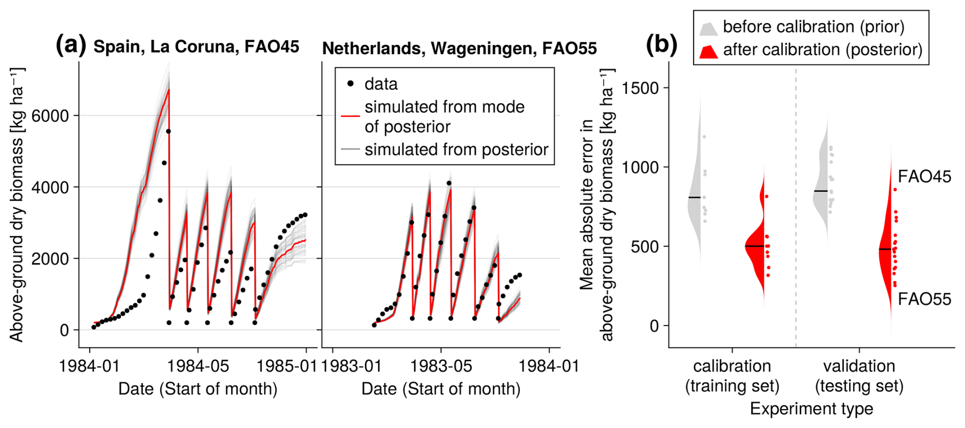
Figure 4Time series from the independent validation experiments with the highest (FAO45) and the lowest (FAO55) mean absolute error in predicting the above-ground dry biomass of the FAO dataset (a). Predictions from the mode of the posterior distribution (maximum a posteriori estimate) and predictions from draws of the posterior distribution are shown to compare with the measured above-ground biomass. In addition, the mean absolute error between the predicted and observed biomass is shown separately for the calibration (training set) and validation (testing set) experiments, both before and after calibration (b). The mean absolute error is calculated for each observation and then averaged across each experiment. The improvement in prediction before calibration, based on the mean error calculated with 50 draws from the prior distribution, is compared to the error after calibration, based on the mean error calculated with 50 draws from the posterior distribution.
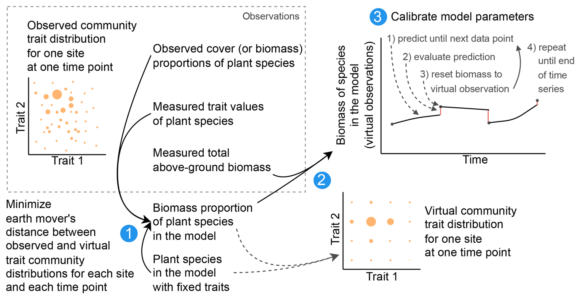
Figure 5Calibration workflow. For the Biodiversity Exploratories dataset, we reduced the number of species from 70 to 25 to lower the computation time in the calibration. We created virtual observations for the 25 species by finding the biomass proportion of the 25 species so that the community trait distribution closely resembles the trait distribution of the community with 70 species (step 1). The biomass proportion of the 25 species can be multiplied by the measured total biomass to create virtual observations for our modelled species (step 2). For the calibration of the global model parameters, the model can be used to simulate a trajectory for one parameter combination. The simulated trajectory is compared with the virtual observation to calculate the likelihood and then reset to the virtual observation. Due to the resetting, we can evaluate how good the model is in predicting from one observation to another. Starting from the second data point, we evaluate the likelihood of minimizing the influence of the initial values, which were not calibrated (step 3). The resetting is not used for the evaluation of the model after the calibration. For the calibration with the FAO dataset, only one species was grown and is simulated, and therefore we only used step 3 for the calibration.
After the calibration, our model can reproduce the seasonal patterns for the species Lolium perenne for independent validation sites across Europe to satisfactory degree (see Fig. 4). The mean absolute error in above-ground biomass was reduced from approximately 750 kg ha−1 of the prior to 500 kg ha−1 of the mode of the posterior (respectively the median of all validation experiments). The uncertainty in the posterior estimates of parameters was reduced greatly compared to the prior (see Figs. F1 and F2). Therefore, the uncertainty in the prediction from the prior compared to predictions from the posterior was also clearly lowered (see Fig. F3).
We conducted a local sensitivity analysis to identify the parameters to which the above-ground biomass of Lolium perenne is most sensitive (see Table F12 for details). The analysis revealed that the most sensitive parameters were those relating to the processes of radiation use efficiency (γRUEmax, γRUE,k, γRAD,1, and αRUE,cwmH), seasonal adjustment for growth (ζSEAmin and ζSEAmax), and senescence (βSEN,sla and αSEN), indicating that small variations in these parameter values lead to substantial changes in the above-ground biomass of Lolium perenne.
3.2 Biodiversity Exploratories dataset – dynamics of community traits and biomass
Second, we used data from the Biodiversity Exploratories project (Fischer et al., 2010). This is an observational dataset of permanent grassland sites from three different regions in Germany, and we used the subset from 2006 to 2022. Farmers documented their land-use practices, and vegetation composition and above-ground biomass were documented annually by researchers. We assessed whether our model could reproduce patterns in total biomass production and in the development of the community trait distribution. We used site-specific climate, management, and soil data (for details on data preparation and references, see Appendix C). In total, 150 sites are included the project. We selected those that were mainly used as meadows (mown) or as a mixture of pasture (grazed) and meadow. We excluded those sites that were used as pasture only, resulting in 92 sites over all three regions. We decided to exclude the pasture sites because farmers often decided to provide supplementary feeding on these sites, and the information on supplementary feeding is not detailed enough to be included in the simulation model. The 82 sites were split into 12 sites for calibration and 70 sites for validation (see Tables F9, F10, and F11). For calibration, we selected four sites from each of the three regions, some of which were mown only, while others were grazed and mown. We calibrated parameters of the water growth reducers ( and δWAT,rsa), nutrient growth reducers (, , δNUT,rsa, and δNUT,amc), investment into roots (κROOT,rsa and κROOT,amc), and the reference traits that influence all just-mentioned processes (ϕTRSA and ϕTAMC). All other parameters were kept constant and are based on literature, based on the calibration with the FAO dataset, or are set manually by comparing simulated trajectories with measured data of the calibration sites.
We compiled trait data for 70 plant species that occurred in the Biodiversity Exploratories sites, partly from measurements from the project and partly from trait databases (for details, see Appendix C). For the calibration, we wanted to lower the computation time. That is why we reduced the number of plant species to 25, by applying hierarchical clustering and calculating the mean trait values for the 25 groups (for details, see Appendix C1). Lowering the number of species did not change the general patterns in community dynamics (see Fig. F4). We derived virtual observations for these 25 virtual plant species by finding a community trait distribution with the 25 virtual species that closely resemble the community trait distribution with the 70 species by minimizing the earth mover's distance (also called the Wasserstein distance; Rubner et al., 2000) between these two community trait distributions (for details about distance between community trait distributions, see Appendix D). Thereby, we optimized the relative abundance of the 25 virtual species (see step 1 in Fig. 5) and calculated the biomass of each virtual species by multiplying the relative abundance by the total biomass (see step 2 in Fig. 5). These virtual observations help to reset the biomass of the simulated species after the evaluation of the likelihood for one time point (see step 3 in Fig. 5). We used a likelihood function based on a normal distribution with zero mean, where the distance between the simulated and the observationally derived community trait distribution (our virtual observations), as calculated by the earth mover's distance, is treated as the data, and the variance is a parameter estimated during calibration. We did not use the total above-ground biomass in the calibration but evaluated it after the calibration. We used the same Markov chain Monte Carlo method as for the calibration with the FAO dataset to derive the posterior distribution for the parameters.
Each species is initialized with the same above- and below-ground biomass (200 kg ha−1) and a height equal to half of their maximum height. This sets the total biomass at a rather high initial value (5000 kg ha−1 of above-ground biomass in winter, see Fig. 7). Environmental conditions, management practices, and biotic interactions with other plant species lead to the site-specific community assembly. While the biomass of most simulated species decreases rapidly due to their functional traits, the biomass of a few species increases over time.
The calibration resulted in a slight decrease in the mean absolute error for predicting the community trait distribution (see Fig. 6) and greatly reduced the mean absolute error for predicting the above-ground biomass (see Fig. 7). The time series of the community-weighted mean traits for the independent validation sites with the lowest distance between predicted and observationally derived community trait distribution (AEG41 in Fig. 6) show that the general trends are captured well for all traits except the root surface area per below-ground biomass. For the site with the highest error in predicting the community trait distribution (AEG31 in Fig. 6), the trend for the most community-weighted mean traits are not well captured. The development of the whole community trait distribution over time for the same sites show that the simulated functional diversity is lower than the observed functional diversity (for variance in the community trait distributions, see Figs. F8, F9, and F10). For most data points, the simulated and measured total above-ground biomass at the independent validation sites with the highest and lowest predictive error correspond closely (see Fig. 7).
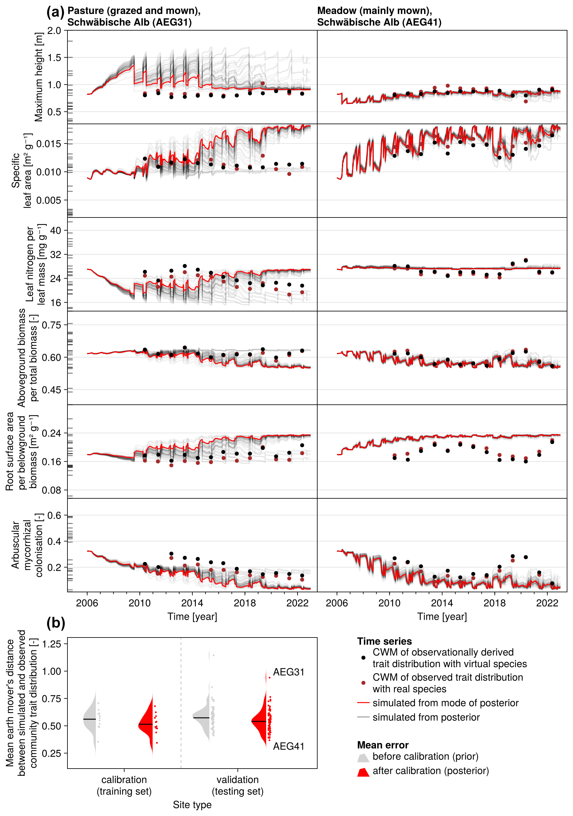
Figure 6Time series of the community-weighted mean trait values for the independent validation sites with the highest (AEG31) and the lowest (AEG41) mean absolute error for the distance between simulated and observationally derived community trait distribution (a). Predictions from the mode of the posterior (maximum a posteriori estimate) and from draws from the posterior distribution are shown in order to compare them with the observationally derived community-weighted mean traits. In addition, the mean absolute error between predicted and observationally derived community trait distribution is shown separately for the calibration (training set) and validation (testing set) sites, both before and after calibration (b). The mean absolute error is calculated for each observation and then averaged across each site. The predictive performance before calibration, based on the mean error calculated with 50 draws from the prior distribution, is compared to the error after calibration, based on the mean error calculated with 50 draws from the posterior distribution.
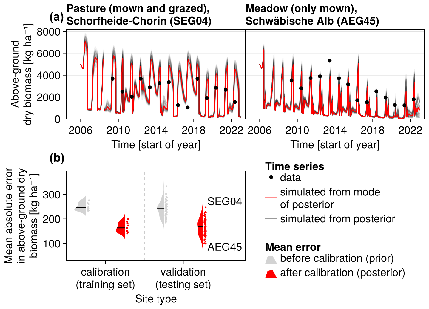
Figure 7Time series from the independent validation sites with the highest (SEG04) and the lowest (AEG45) mean absolute error in predicting the above-ground dry biomass of the Biodiversity Exploratories dataset (a). Predictions from the mode of the posterior distribution (maximum a posteriori estimate) and draws from the posterior distribution are shown in order to compare them with the measured above-ground biomass. In addition, the mean absolute error between predicted biomass and measured biomass is shown separately for the calibration (training set) and validation (testing test) sites, both before and after calibration (b). The mean absolute error is calculated for each observation and then averaged across each site. The predictive performance before calibration, based on the mean error calculated with 50 draws from the prior distribution, is compared to the error after calibration, based on the mean error calculated with 50 draws from the posterior distribution.
We applied a local sensitivity analysis and calculated the sensitivity of the total above-ground biomass to small changes in parameter values (for details, see Table F13). We confirmed that the total above-ground biomass is most sensitive to changes in parameters dealing with senescence (ϕsla, αSEN, and βSEN,sla), the calculation of the permanent wilting point and the water-holding capacity (βCLY,PWP, βSLT,WHC, and βCLY,WHC), radiation use efficiency (γRUEmax, γRUE,k and αRUE,cwmH), and seasonal growth adjustment (ζSEAmax and ζSEAmin).
4.1 Validation of GrasslandTraitSim.jl
The validation of the GrasslandTraitSim.jl model demonstrated its ability to relate the morphological traits of plant species to their species-specific physiological and demographic rates. Changes in these rates lead to changes in species biomass and, consequently, changes in plant community composition. We proved that the model could satisfactorily reconstruct seasonal biomass production for one species, biomass production of plant communities, and (with minor limitations) functional community composition for various grassland sites.
One of the key advantages of our modelling approach is that we can compare the simulated morphological trait distributions with measured morphological trait distributions at the community level. In contrast to previous grassland models (e.g. DynaGraM; Moulin et al., 2021 or GRASSMIND; Taubert et al., 2012) that require demographic or physiological rates as species-specific parameters, our model requires only commonly measured morphological traits (compare Fig. 2). In this way, our model can be applied to a much larger set of species and communities for which such trait data are available from on-site measurements or databases.
In our model, we tried to keep a balance between a model that can reproduce the basic patterns in biomass production and functional community composition but does not have too many global parameters, so that it is possible to calibrate all parameters with datasets that are readily available. However, already with the complexity that we presented here, it was not possible to calibrate all global parameters using the Markov chain Monte Carlo method at once. We had to manually fix some parameter values beforehand, and we had to set informative priors on the parameters so that all chains from random starting positions of the prior distribution converged to the posterior distribution within a reasonable number of iterations.
In general, it was much easier to calibrate the model parameters with the FAO dataset, because biomass was measured weekly rather than annually, as was the case with the Biodiversity Exploratories' observations of biomass and composition. Annual observations are not optimal because many different trajectories, simulated by sets of parameter values, can lead to the same simulated point after 1 year. This highlights the need for datasets with several measurements per year for the calibration of process-based grassland models (Taubert et al., 2020). These detailed datasets could also reduce the widespread problem of parameter identifiability in the calibration of ecosystem models (Luo et al., 2009).
Another limitation of the Biodiversity Exploratories dataset is that we used species mean traits, derived from the project or from trait databases, to calculate the community trait distribution (see Appendix C). However, using species mean traits results in the loss of intra-specific trait variability from the observations. We expect the realized community trait distributions to vary more between sites than is reflected in the dataset (Violle et al., 2012; Siefert et al., 2015).
We included grazing in our model because grazing is an important land-use factor in semi-natural grasslands. Some of the grassland models did not take this factor into account (see Table 1 or F2). However, in this study, we were not able to fully calibrate and evaluate grazing in our model, as the sites of the Biodiversity Exploratories lack accurate data to quantify supplementary feeding. Supplementary feeding is an important factor, for example, on year-round grazing sites.
For the independent validation site with the highest error in the FAO dataset (FAO45 in Spain, see Fig. 4), our model predicts too high above-ground biomass in spring. Thereby, we see that the model is not flexible enough to simulate production in a very wide range of regions. Our step function for seasonal growth adjustment assumes that the growth increases in spring after 200 °C have been accumulated (see Eq. 32). This might be a reasonable assumption for Lolium perenne in the Netherlands but not for sites in Spain. The strong growth starts too early for the site in Spain. For the calibration of the LINGRA model with the same dataset, it was assumed that species-specific parameters are different for the northern and southern sites (Bouman et al., 1996). We did not calibrate the model here for spatial subsets of the sites, as we wanted to analyse whether our model is in general applicable to a variety of sites.
4.2 Discussion of the concept
We chose the morphological functional traits that represent the main trade-offs in plant physiology. Rather than reflecting one process in detail with many traits (e.g. more traits dealing with water stress, such as stomatal conductance and rooting depth), we aimed to represent the following main trade-offs of plants: (1) the slow–fast continuum of the leaf economic spectrum states that plants with thinner leaves have a higher light-use efficiency per unit of biomass but also a higher senescence rate (as reflected by specific leaf area; Reich et al., 1992; Wright et al., 2004). (2) Taller plant species can overtop other plant species and are therefore less affected by shading. However, they are more susceptible to mowing and grazing (as reflected by maximum plant height; Díaz et al., 2007; Klimešová et al., 2008). (3) Investing in roots and mycorrhizae enhances nutrient and water uptake, but this comes at the cost of maintaining fine roots and the collaboration with mycorrhiza (as reflected by above-ground biomass per plant biomass, root surface per below-ground biomass, and arbuscular mycorrhizal colonization rate; Reich, 2014; Prieto et al., 2015; Bergmann et al., 2020).
To some extent, our model can simulate intra-specific trait variability based on the functional representation rather than species identity. In our model, two simulated species can represent one species in the real world that exhibits different traits at different sites. However, this approach is not applicable to plant species whose traits change dynamically depending on variable environmental conditions. Furthermore, our model does not reflect changes in traits during the life stages of plant species.
The number of co-existing species (e.g. with biomass > 2 %) is rather low, with three to five species accounting for most of the biomass in most scenario analyses. This is a common challenge in grassland models. For example, in a model comparison study with the GRASSMIND and LPJmL models, it was noted that in a two-species simulation, one species always accounted for most of the biomass (Wirth et al., 2021). We noticed that by including a density-dependent senescence rate (not shown in the model equations above), the simulated functional diversity is increased, and the distance between modelled and observed community trait distributions can be lowered. A density-dependent senescence rate can be explained, for example, by negative plant–soil feedbacks (Bonanomi et al., 2005; Liu et al., 2022; Goossens et al., 2023). This shows the potential to explore in future studies how the incorporation of co-existence mechanisms can lead to more realistic predictions of functional community composition.
We argue that our model is well suited for analysing the effects of management (grazing, mowing, and fertilization), edaphic factors (soil nitrogen, permanent wilting point, and water-holding capacity), and climatic factors (temperature, radiation, potential evapotranspiration, and precipitation) on the productivity and functional composition of diverse plant communities of temperate semi-natural grasslands. We envisage the model as a useful tool for conducting scenario analyses (e.g. what would happen if the input X were to change and why?), rather than as a model with superior predictive performance compared to conventional statistical models. For example, the influence of management type and intensity on achieving a balance between creating highly productive grasslands and maintaining plant diversity could be analysed. Furthermore, the influence of the initial species composition on the productivity under fluctuating climate conditions (e.g. years with drought) could be studied by answering the question of whether a more diverse community can buffer extreme climatic events. Moreover, we consider the potential application of including or excluding certain processes (e.g. a specific transfer function, which links traits to demographic rates) and analyse whether the agreement between simulations and measured data improves.
We presented GrasslandTraitSim.jl, a process-based model that can be used to simulate the effects of land use and climate change on the plant functional composition and biomass production of permanent semi-natural grasslands. We have extended the approach of Chalmandrier et al. (2021) by linking measurements of morphological plant traits with demographic and physiological species-specific processes. Our model uses only morphological traits as species-specific inputs to simulate the biomass of many plant species over time. Therefore, the study is a step towards modelling highly diverse plant communities in grasslands. Further simulation studies – for example, the analysis of different land-use scenarios – are required to fully explore the potential of the GrasslandTraitSim.jl model. We hope that the accompanying documentation, tutorials, and open-source code will encourage collaboration and discussion on this topic.
The response curves (growth reducers) REDts for different nutrient and water availabilities, denoted as Rt, are implemented via logistic equations with a minimum of zero (no growth is possible) and a maximum of 1 (no growth reduction). While the species-specific part of the response curves is implemented by different inflection points , the slope βRED is the same for all species:
We then used another logistic equation that relates the trait values to the inflection point of the response curve. We wanted to control how much the response curves should differ when the trait values differ from ; this is implemented with the parameter δRED. The equation could be written as
However, these equations and their parameters , , and are hard to understand and to interpret, therefore we reformulated the equation. Instead of calculating the inflection point directly, we calculated the growth reduction at 0.5 of the maximal resource availability:
This has the advantage of having natural boundaries , because the growth reduction cannot be larger than 1 (REDts=0) or lower than zero (REDts=1). We introduce one parameter αRED,05, which is the growth reducer for the mean trait ϕtrait at half of the maximal resource availability:
and rearranged the equation to
This leads to an equation that we can use to calculate the growth reducer for all trait values at half of the maximal resource availability:
Now, we need again the full equation to calculate the growth reducer for any resource availability. We use Eq. (A1) and solve for with REDts=0.5:
to get the inflection point :
Thus, the full equation to calculate the growth reducer for any resource availability is
and with everything combined and simplified,
Note the species-specific inflection point is in square brackets.
The model is implemented as a Julia package and can be used with the Julia programming language (Bezanson et al., 2017). It can be used on all major operating systems (Linux, MacOS, Windows). The model can be run on computers with low hardware requirements. For example, a 10-year simulation involving 70 species typically takes less than 0.5 s to run on a standard personal computer. A graphical user interface allows you to manually change parameter values and see the influence of each parameter on the simulation results (explained in more detail in the online documentation, see data accessibility statement). The model can be run on headless systems, but then the graphical user interface is not available. Throughout the model, units are used directly in the programming code using Unitful.jl, making the model easier to understand and debug. The outputs of the model have labelled axes using DimensionalData.jl, making it easy to know which is the space, time, or species axis. The package has extensive online documentation with all the equations, tutorials on how to set up the input data, and how to analyse the output (see data accessibility statement). For each equation, there are interactive plots to visualize the relationship between the variables and the influence of the parameters. Flow charts are also available online to give a quick overview of the sub-processes. The model version described here can be installed in Julia using import Pkg; Pkg.add("GrasslandTraitSim", version = "1.0.0"). The newest version can be installed using the same command without the version argument. All dependencies will be installed with this command. The model is open source and licensed under the GNU GPLv3. Contributions are welcome and can be made via GitHub. The development of the model is hosted at https://github.com/felixnoessler/GrasslandTraitSim.jl (last access: 8 September 2025), and new versions will be published in the General Julia package registry.
We compiled input data for the model from different sources. Management data were used directly from the Biodiversity Exploratories project (timing and intensity of grazing, timing, and height of mowing events and total fertilization of nitrogen per year; Vogt et al., 2024). The exact dates of grazing were not available, only the type of grazing, the number of days, and the start and end month of a grazing period. We assumed different numbers of consecutive grazing days (2 for rotational grazing type I – “Portionsweide”, 5 for rotational grazing type II – “Umtriebsweide”, and all days for permanent grazing) and distributed them equally over the whole grazing period. Potential evapotranspiration was used from AMBAV, an agro-meteorological model that outputs “potential evaporation over grass” from weather stations in the three regions (DWD Climate Data Center, 2019) and is therefore the same for all sites of one region. Air temperature and precipitation were obtained for each site from the Biodiversity Exploratories project (Wöllauer et al., 2023). Photosynthetically activate radiation (PAR) was downloaded with a 3 h resolution from Wang (2021), and the daily sum of PAR was obtained by calculating the integral of a quadratic regression to the PAR values. We calculated the PAR values per region. We created region-specific PAR inputs due to the coarse resolution of the PAR data. Soil texture (Schöning et al., 2021c), rooting depth (Herold et al., 2021), bulk density (Schöning et al., 2021d), and organic matter content (Schöning et al., 2021b) were used from soil-sampling campaigns of the Biodiversity Exploratories project. The total nitrogen concentration was aggregated from 4 years to get a mean overall total nitrogen concentration (Schöning et al., 2021b, e, a; Schöning, 2023). The trait data were compiled from species that are present in the grasslands of the Biodiversity Exploratories project. Leaf area and leaf dry weight were sampled from individuals from sites of the Exploratories project (Prati et al., 2021) to calculate the specific leaf area. The root surface area per below-ground biomass, arbuscular mycorrhizal colonization rate, and above-ground biomass per total biomass were obtained from individuals that were grown in a greenhouse experiment on sand (Bergmann and Rillig, 2022). The maximum height was obtained from Jäger et al. (2017) and the leaf nitrogen per leaf mass from the TRY database (Kattge et al., 2020, mainly from Gubsch et al., 2010; Pakeman et al., 2008; Schroeder-Georgi et al., 2016). We decided to set leaf biomass per above-ground biomass to 80 % for all species, as values for the trait leaf biomass per plant biomass were not available for many species. For 70 species, we had values for all the traits. We used a reduced set of 25 species as input for the simulation (see Appendix C1). During initialization, the initial above-ground and below-ground biomass of 5000 kg ha−1 was evenly distributed across all species. The initial height was set to half of the maximum height of each plant species. The initial soil water content was set to 180 mm, which assumes no drought stress in the beginning of the simulation. For the calibration and validation data, we used the cut above-ground biomass and the cover to compare observed and simulated community trait distributions. The biomass was cut once per year on every site at a height of 4 cm (Hinderling et al., 2024). Each year, the cover of plant species was estimated on an area of 16 m2 (Hinderling and Keller, 2023). Whereas we used input data from 2006 to 2022, we used only calibration data from 2010 to 2022 to allow for an initialization phase of the grassland model.
C1 Reducing the number of species from 70 to 25 for the Biodiversity Exploratories dataset
For calibration, we reduced the number of simulated species from 70 to 25. We calculated new trait values for the 25 species by forming groups of species with similar trait values and calculating the mean trait values within each of the 25 groups. To do this, we first standardized the trait values by min–max normalization to a range of [0, 1] to give each trait value equal weight in the distance calculation. We then calculated the Manhattan distance between all 70 species. We applied a hierarchical clustering (“hclust” function from “stats” package, R Core Team, 2024), formed 25 groups, and calculated the mean of the non-standardized trait values to obtain the trait values for 25 virtual species. A comparison of the simulated community dynamics with 70 and 25 species showed that lowering the number of species did not change the general community patterns (see Fig. F4).
The earth mover's distance, which is also called the Wasserstein distance, can be used to calculate the distance between two discrete distributions (Rubner et al., 2000; Villani, 2009; Bernton et al., 2019; for application in movement ecology, see Potts et al., 2014; Kranstauber et al., 2017). The cost is computed as the product of the amount of probability mass transported and the distance it is moved. We used the implementation in the Python package “scipy” (“wasserstein_distance_nd” function; Virtanen et al., 2020). With this function, the trait values of both distributions are given as “u_values” and “v_values” (matrices, each row with trait values for one species), and the respective cover or biomass proportions are given as “u_weights” and “v_weights”. We standardized the trait values by z-score normalization () to give each trait an equal weight in the calculation of the earth mover's distance.
For both datasets, we used the Haario-Bardenet Markov chain Monte Carlo with the Python software package PINTS (Clerx et al., 2019). We called our Julia package GrasslandTraitSim.jl from Python. We ran four independent chains for 75 000 iterations (150 000 for the FAO dataset) and discarded the first half of the iterations as warm-up. The first 5000 iterations were used as an adaption-free initial phase. We checked that all four chains converged to the same posterior region by visually examining the trace plots (see Figs. F2 and F7) and by checking that all rhat values were less than 1.01 (not shown; Vehtari et al., 2021). We compared how much the posterior shifted in comparison to the prior densities and interpreted this as how much uncertainty was reduced (see Figs. F1 and F6). We also compared how much uncertainty was reduced while simulating trajectories with GrasslandTraitSim.jl from the prior and from the posterior (comparing the prior predictive with the posterior predictive distribution, see Figs. F3 and F5).
For both datasets, we used the one-step-ahead prediction method (predict until next data point, evaluate prediction, reset state variables to data point, and repeat the procedure). By using this method and not explicitly estimating the hidden state of the above-ground biomass (e.g. by a state space model), we ignored the observational error and only considered the process error. We assumed that the observational error is small and decided to keep the calibration method simpler by not estimating the hidden states.
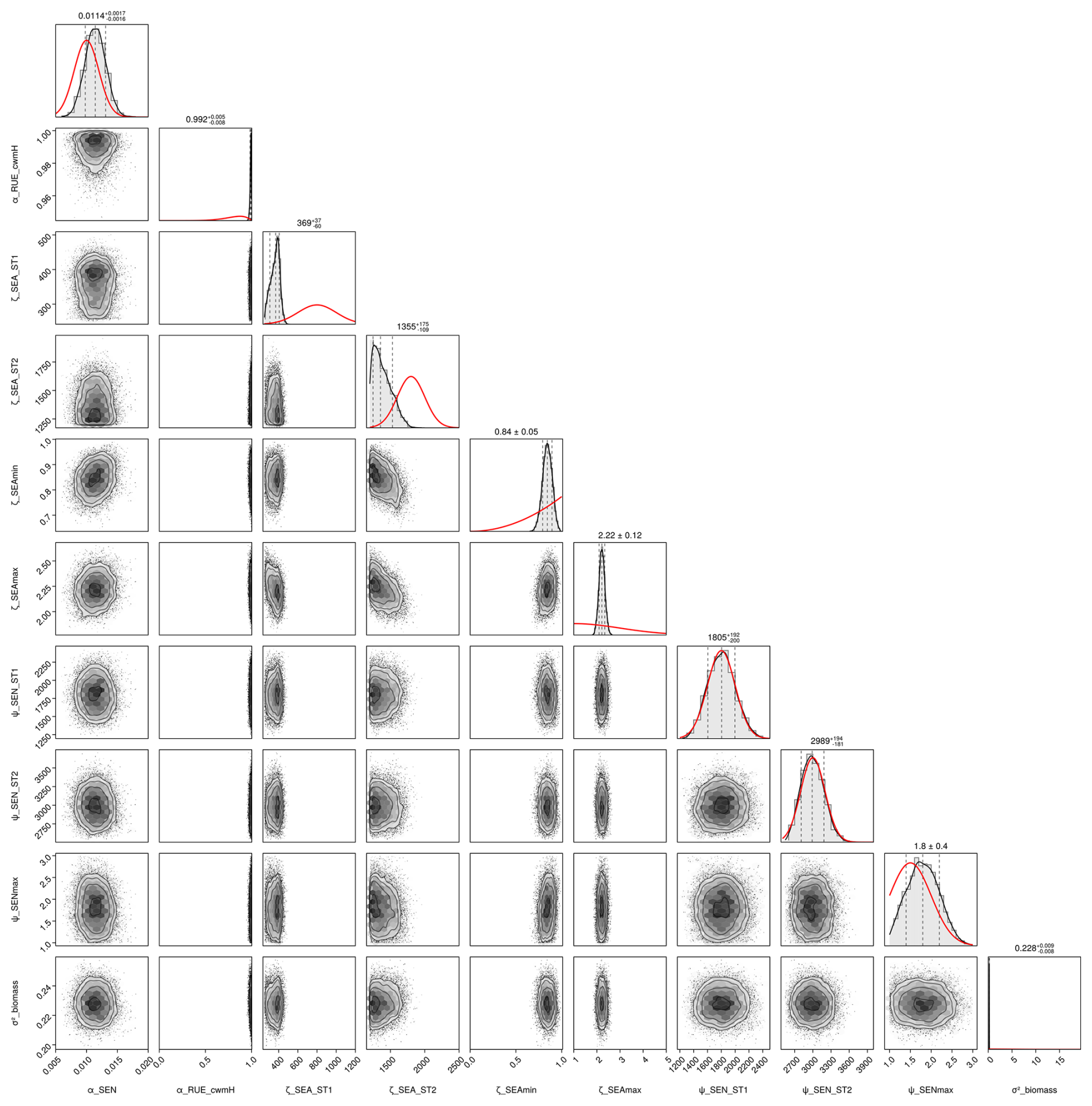
Figure F1Pair plot of the posterior densities for calibration with the FAO dataset. In the right upper plots, the marginal posterior densities (histograms) are shown, together with the prior densities (red lines). The first half of the iterations were discarded as warm-up.
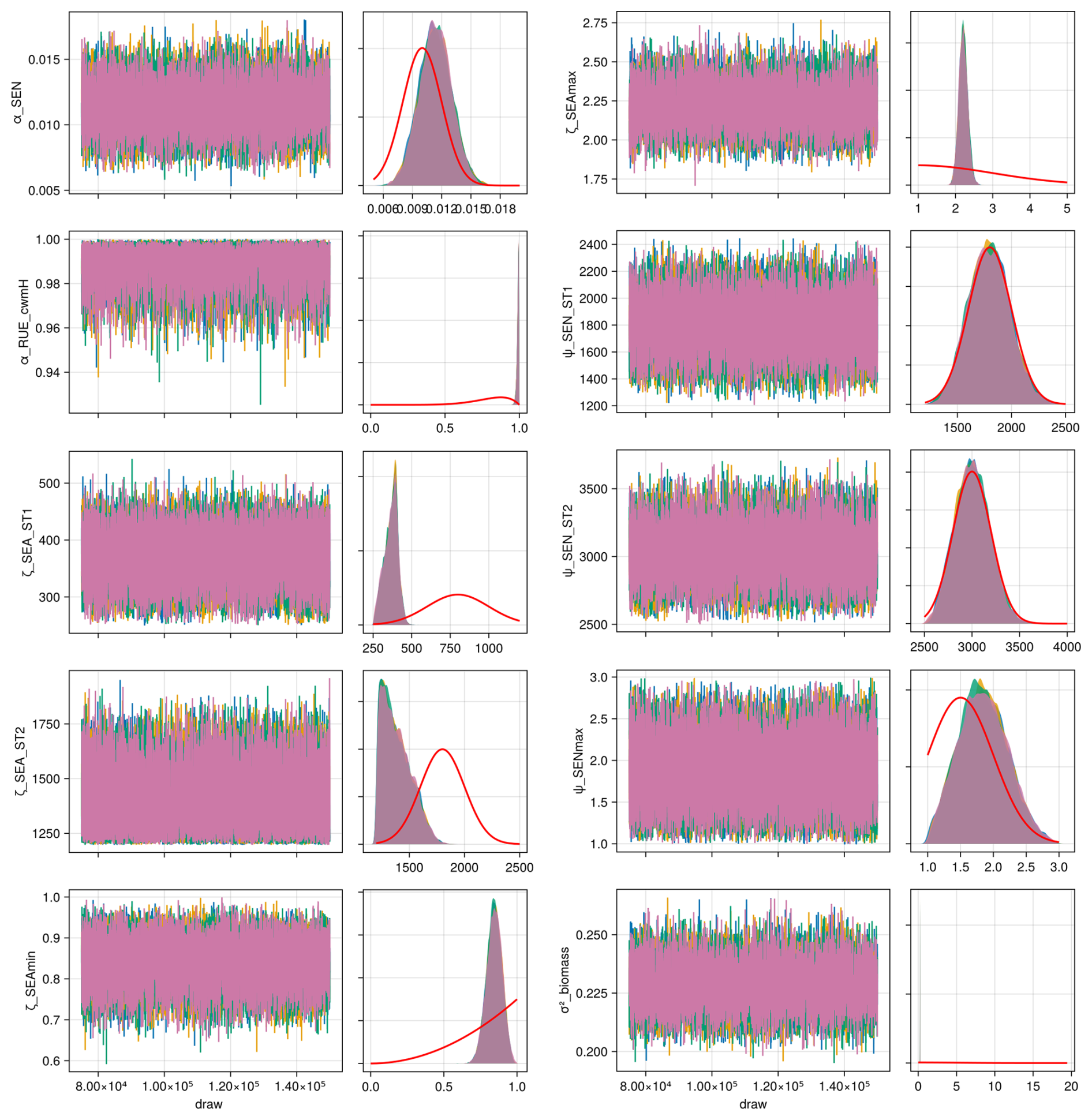
Figure F2Trace plot and prior and posterior densities for calibration with the FAO dataset. Different colours represent the different Markov chains. In the density plot, the prior density (red line) and the posterior densities are visible. The first half of the iterations were discarded as warm-up.
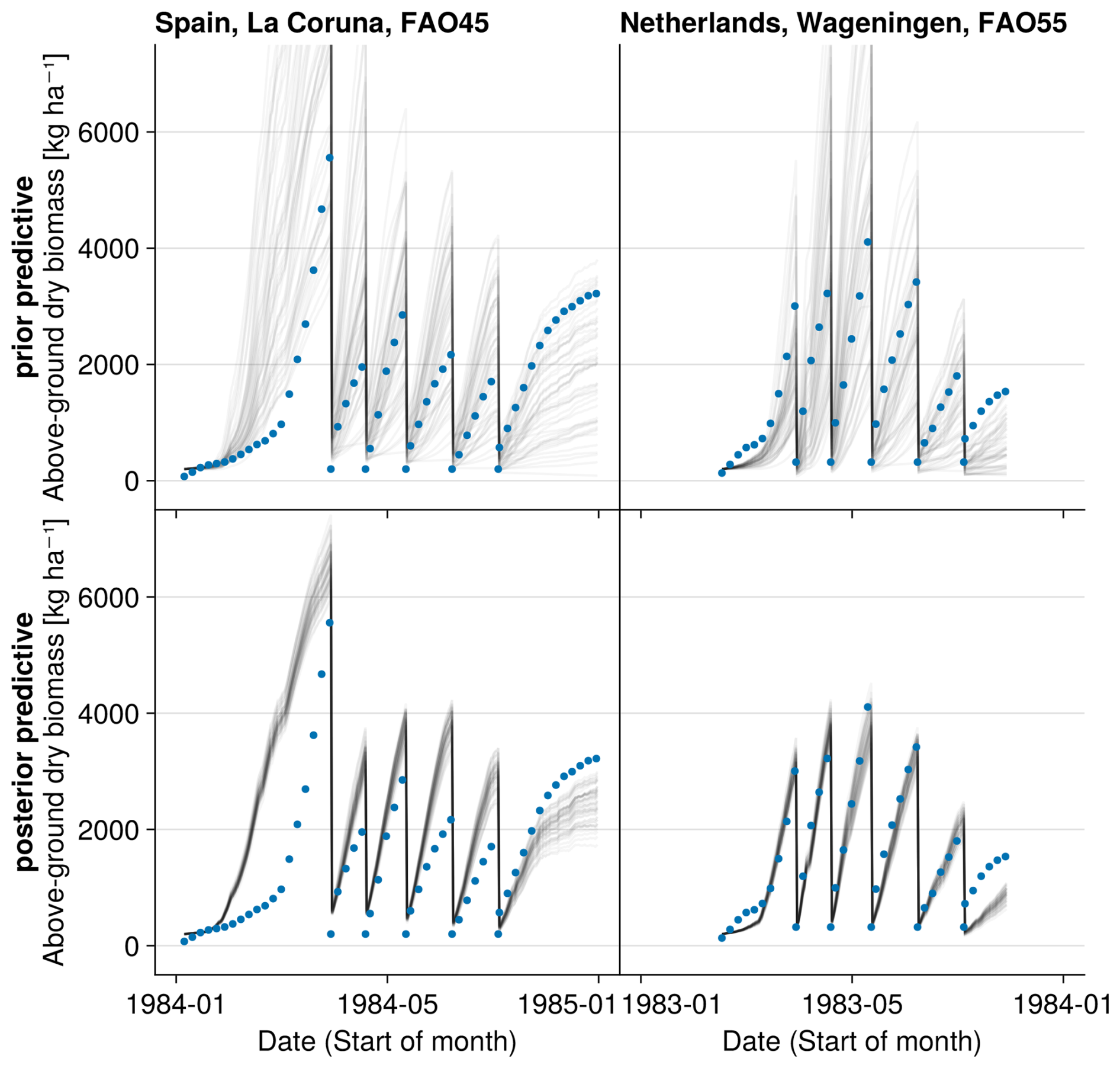
Figure F3Prior and posterior predictive checks for the FAO dataset. Simulations with parameters drawn from the prior distribution or from the posterior distribution (grey lines) are compared to measured above-ground biomass (blue dots).
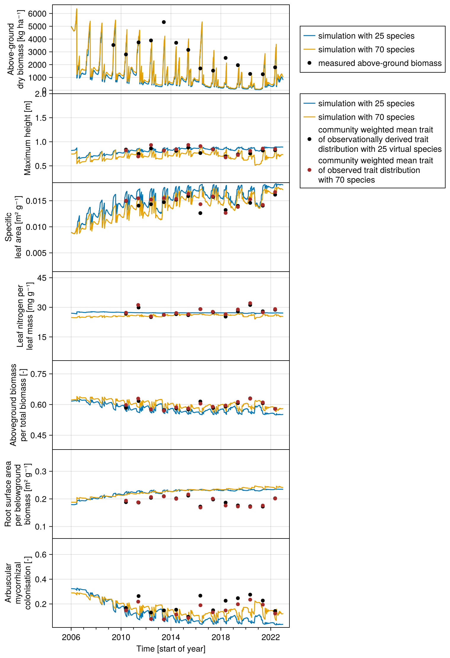
Figure F4Comparison of community dynamics (above-ground biomass and community-weighted mean traits) with 70 species and with the reduced set of 25 species. The trait values of the 25 species were derived by calculating the mean trait values of 25 groups that were built from the dataset with the trait values of all 70 species (see Appendix C1).
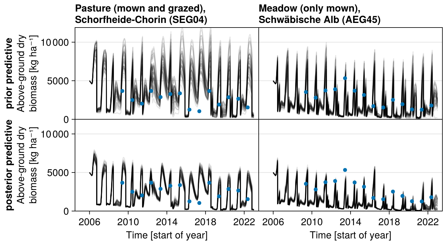
Figure F5Prior and posterior predictive checks for two sites of the Biodiversity Exploratories dataset. The predicted above-ground biomass, based on simulations with parameters drawn from either the prior or the posterior distributions, is compared to the measured above-ground biomass.
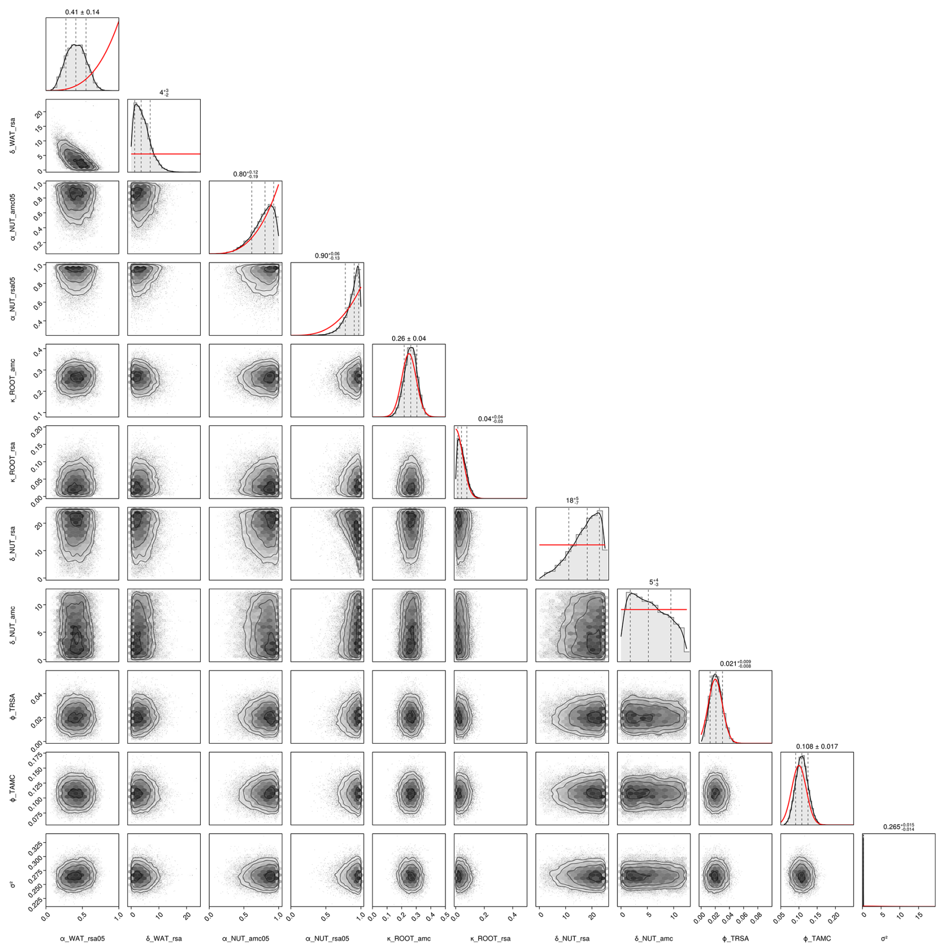
Figure F6Pair plot of the posterior densities for calibration with the Biodiversity Exploratories dataset. In the right upper plots, the marginal posterior densities (histograms) are shown, together with the prior densities (red lines). The first half of the iterations were discarded as warm-up.
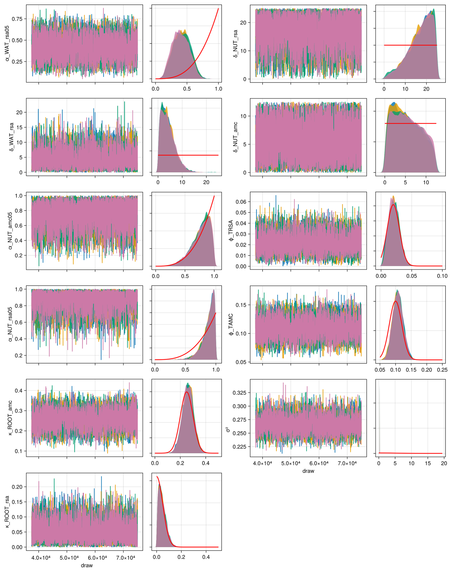
Figure F7Trace plot and prior and posterior densities for calibration with the Biodiversity Exploratories dataset. Different colours represent the different Markov chains. In the density plot, the prior density (red line) and the posterior densities are visible. The first half of the iterations were discarded as warm-up.
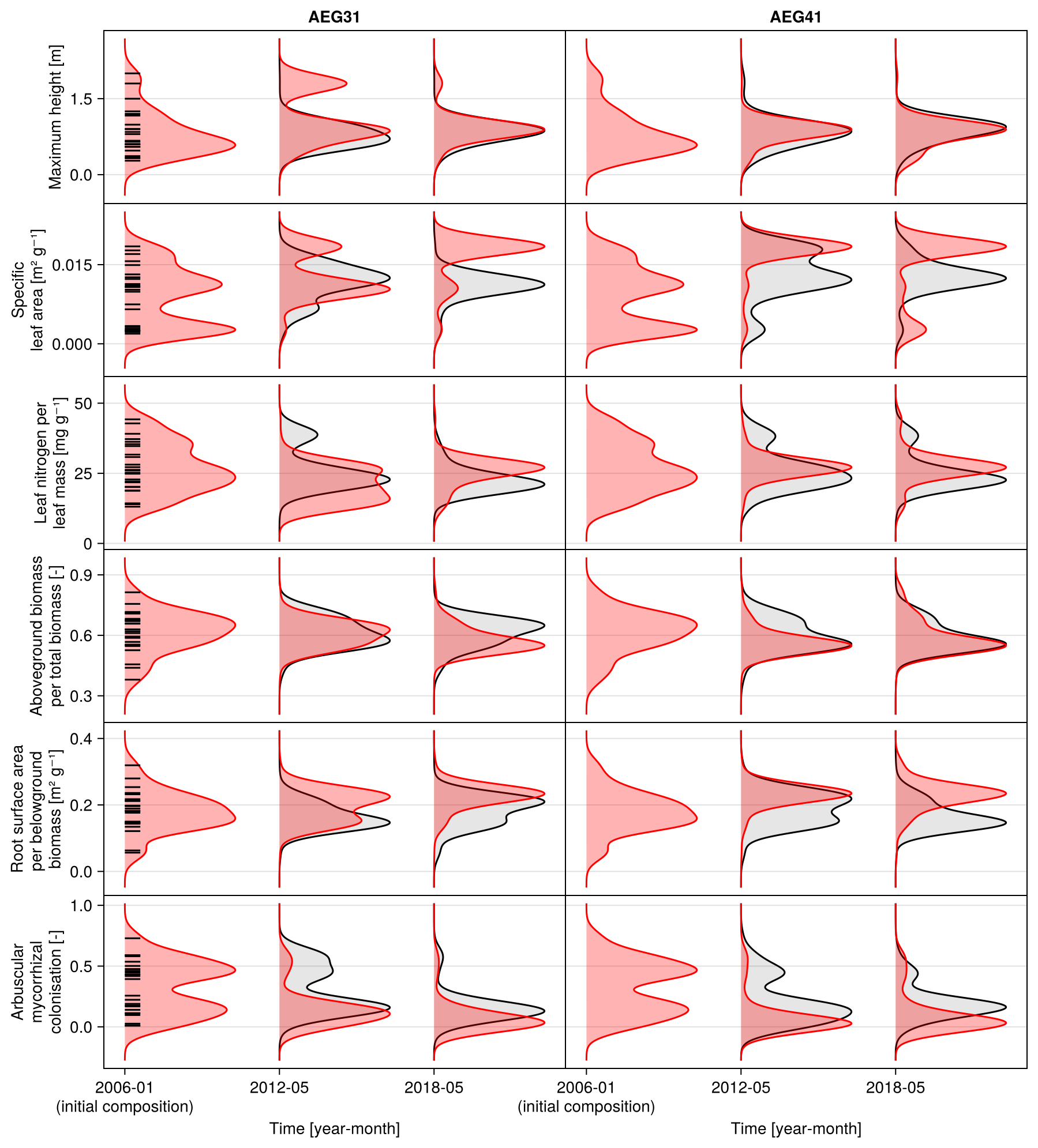
Figure F8Development of the community trait distribution over time for validation sites, with the highest (SEG20) and the lowest (HEG47) mean absolute error for the distance between simulated and observed community trait distribution (for the selection, see Fig. 6). The simulated (red) and observed (grey) densities are calculated using kernel density estimation by including the biomass proportion of the species as weights. The trait values of the species are constant (horizontal black lines on the left). To analyse correlations between traits, the observed and simulated trait distributions are shown in a pair plot for 2018 in Figs. F9 and F10.
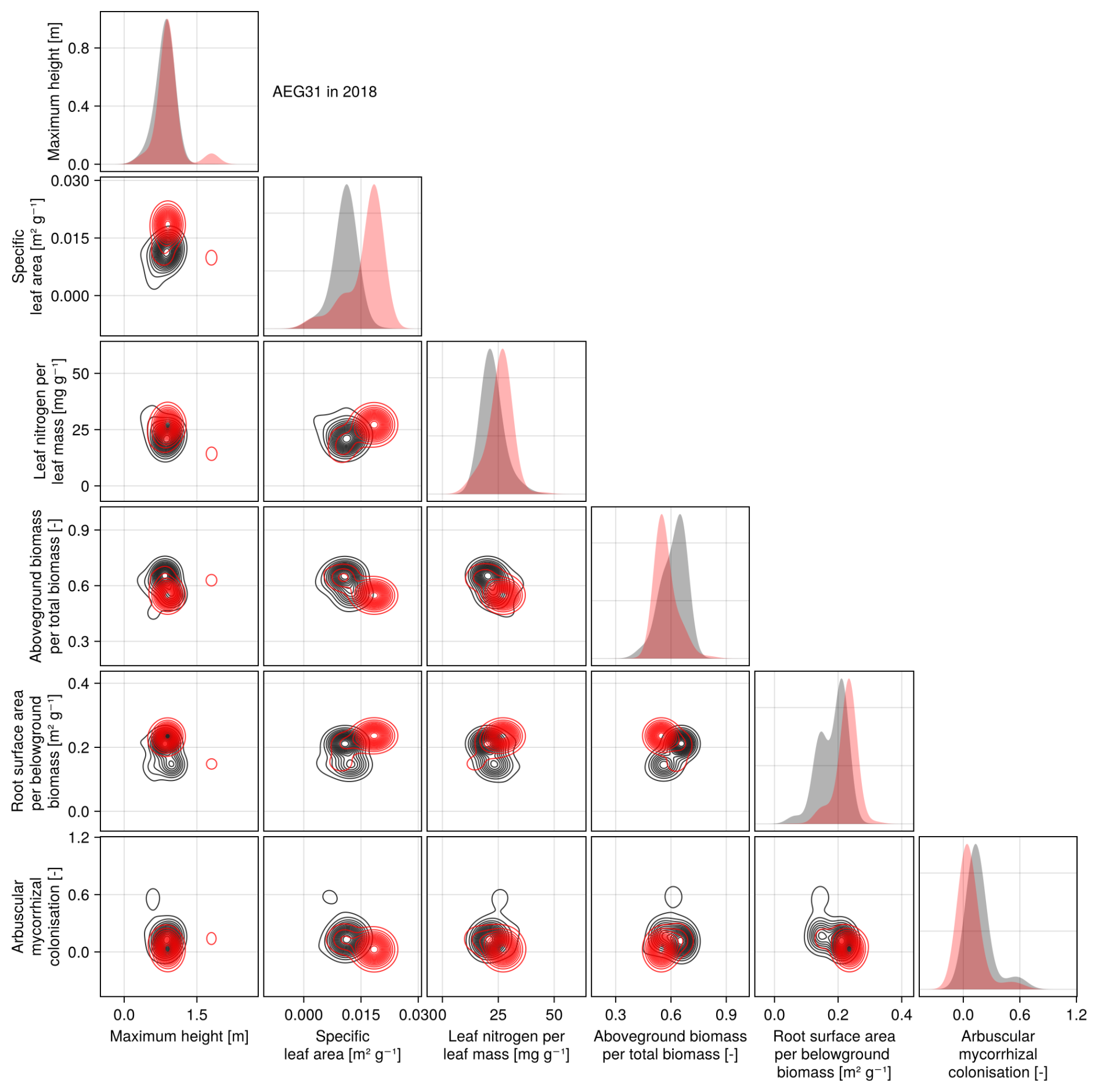
Figure F9Simulated (red) and observationally derived (black) community trait distribution for the grassland site AEG31 of the Schwäbische Alb region (Germany) in 2018. The AEG31 site has the greatest distance between the simulated and the observationally derived community trait distribution over all years (see Fig. 6).
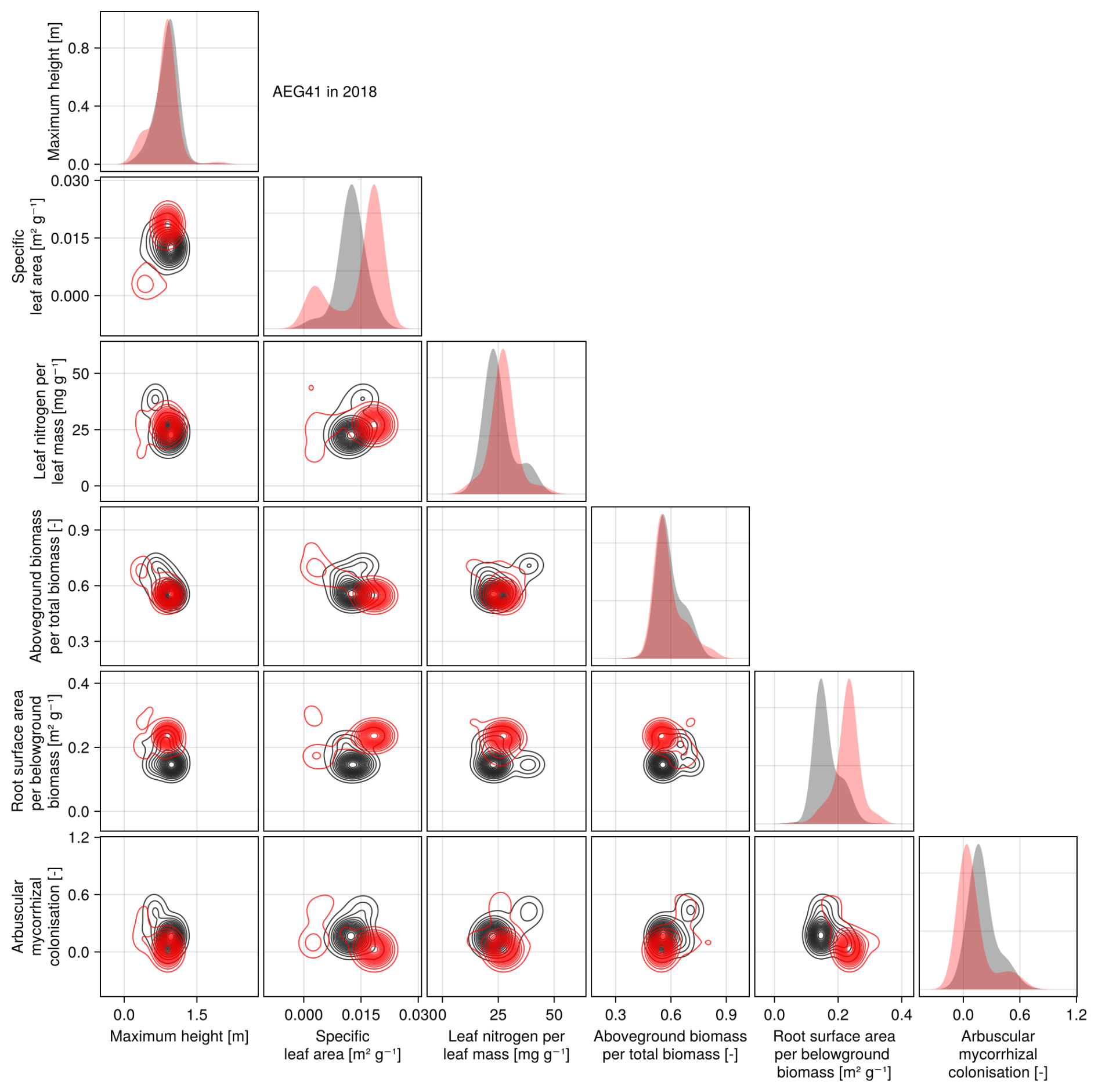
Figure F10Simulated (red) and observationally derived (black) community trait distribution for the grassland site AEG41 of the Schwäbische Alb region (Germany) in 2018. The AEG41 site has the shortest distance between the simulated and observationally derived community trait distribution over all years (see Fig. 6).
Table F1Grassland model overview – general characteristics.
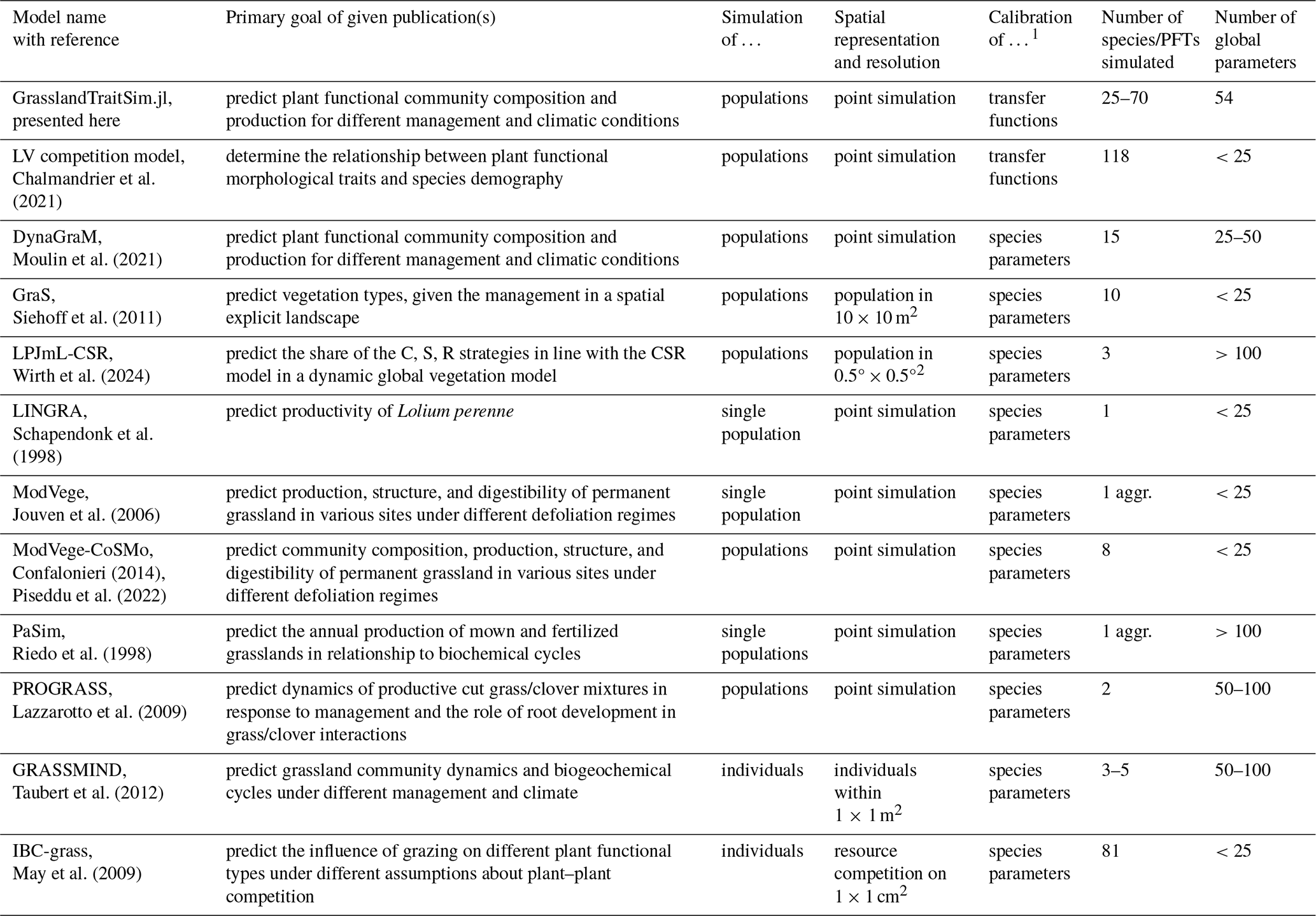
1 We distinguish between models in which parameters of transfer functions mapping morphological functional traits to species demographic rates are calibrated, together with models in which species demographic parameters are calibrated directly (Chalmandrier et al., 2021). 2 LPJmL-CSR can be applied on a global scale but was also used on a higher spatial resolution for smaller areas, e.g. with grid cells of 1 × 1 km2.
Table F2Grassland model overview – ecological and technical details.
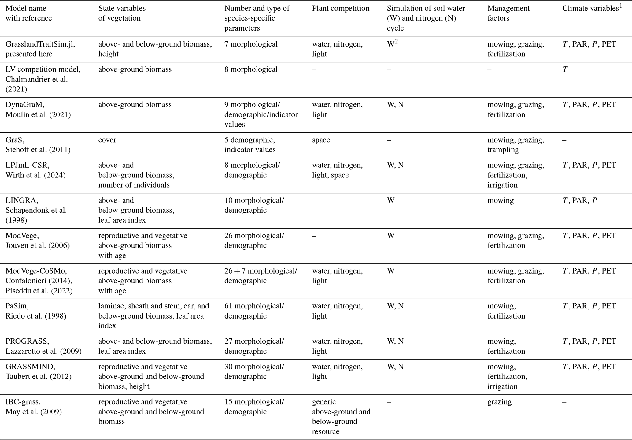
1 We have reviewed whether air temperature (T), photosynthetically active radiation (PAR), precipitation (P), and potential evapotranspiration (PET) are used in a model. Other external climate drivers, even if used in the specific model, are not shown in the table. 2 While the soil nutrient index can change with time and the amount of biomass, the soil nitrogen cycle is not simulated explicitly in GrasslandTraitSim.jl. 3 We define the number of global parameters as all parameters that are not species specific.
Table F3Input variables of the GrasslandTraitSim.jl model. The dimensions of the variables are given in the subscript of the symbols: t per day and s per species.
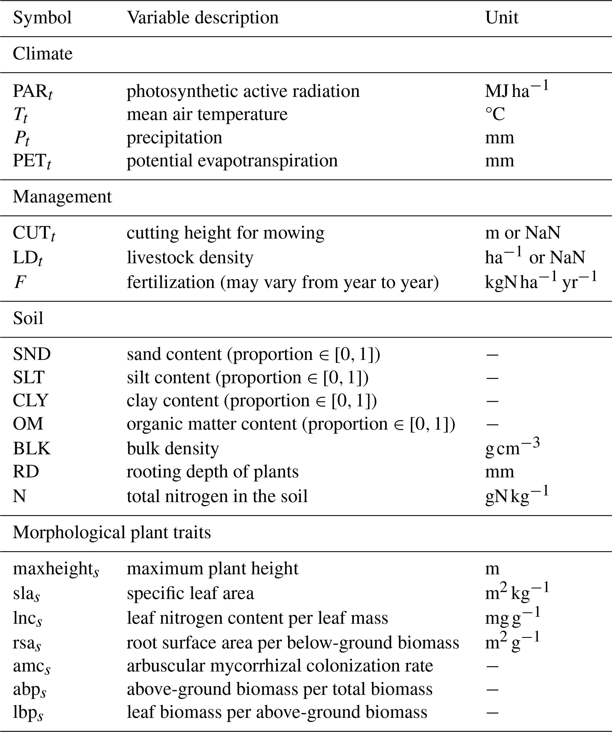
Table F4Parameters of the model and the references for the parameter values. In the reference column, we denote whether a parameter is calibrated with the Biodiversity Exploratories (BE) or the FAO dataset, whether the parameter is set manually by comparing time series with data or if the parameter value is derived from literature. For the parameters calibrated using the FAO dataset, we set prior distributions based on the literature, as shown in Table F6.
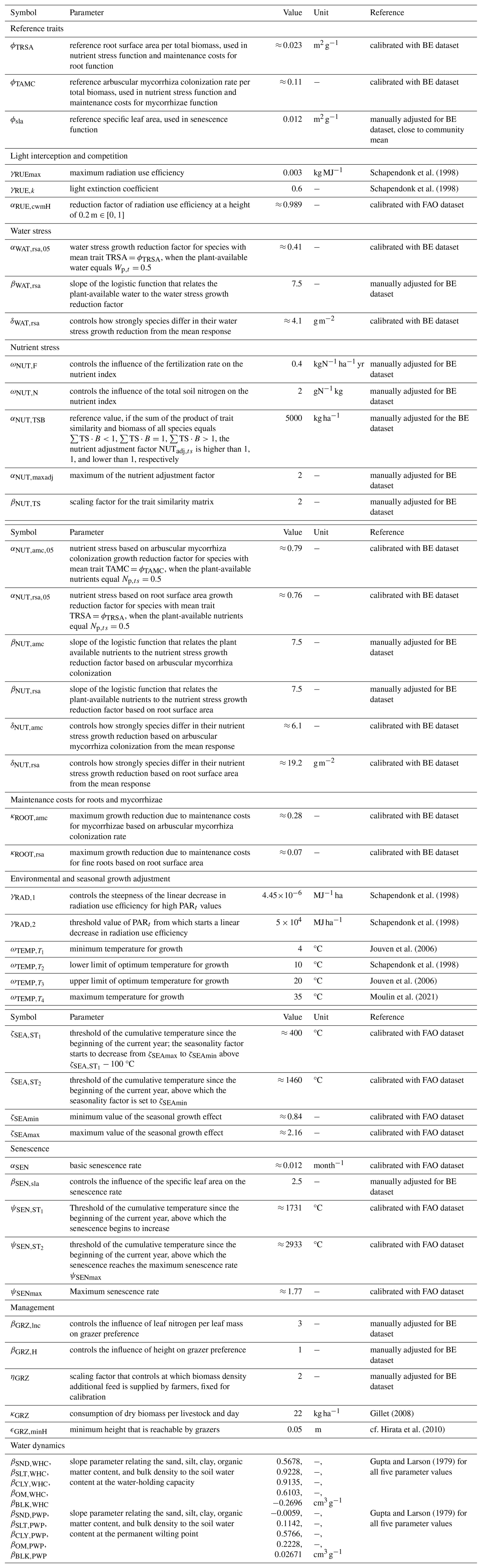
Table F5Overview of the model equations and their references. New means that the equations are newly composed for the grassland model and were not adopted from other grassland models.
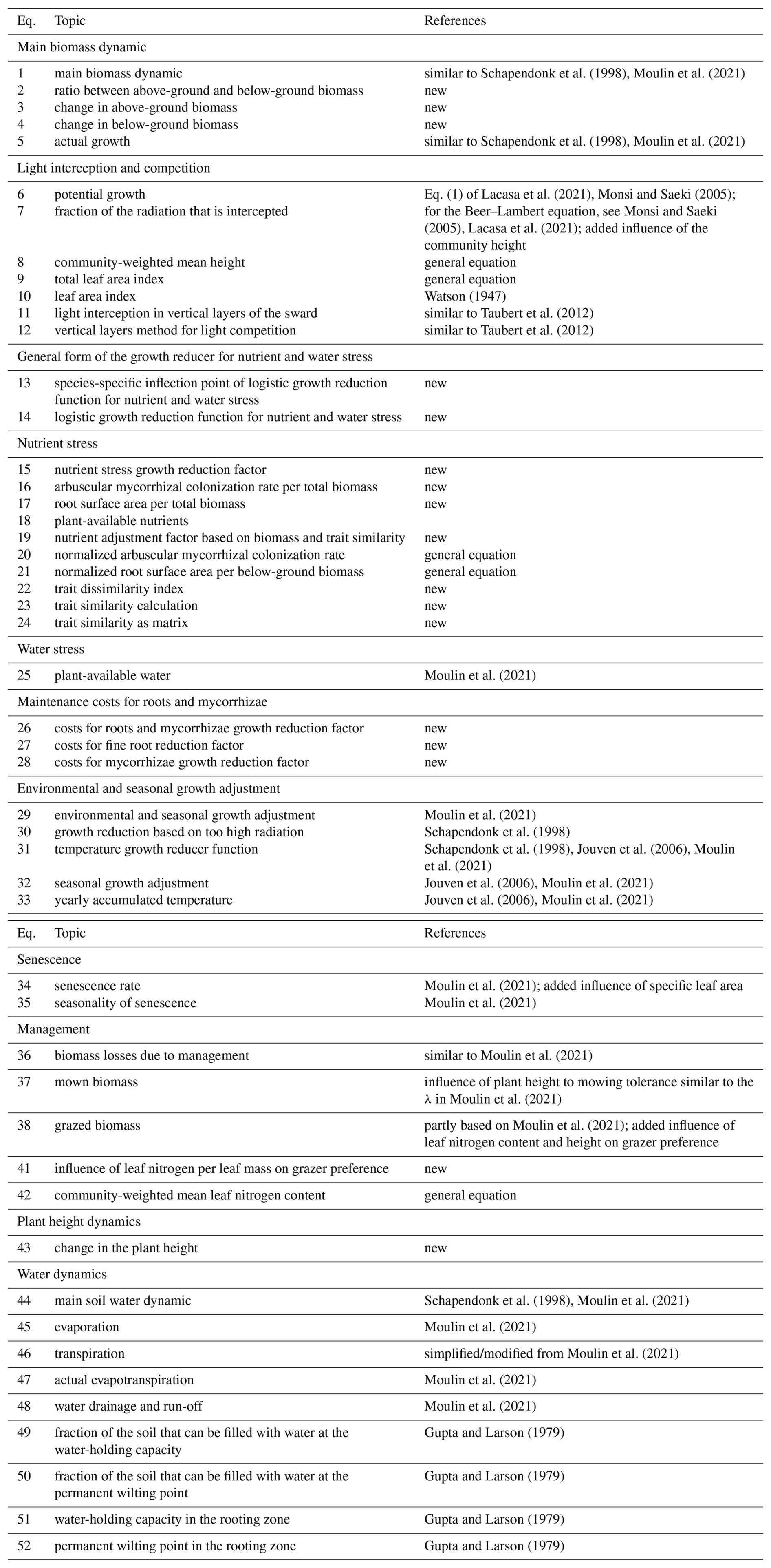
Table F6Prior distributions for calibration with the FAO dataset.
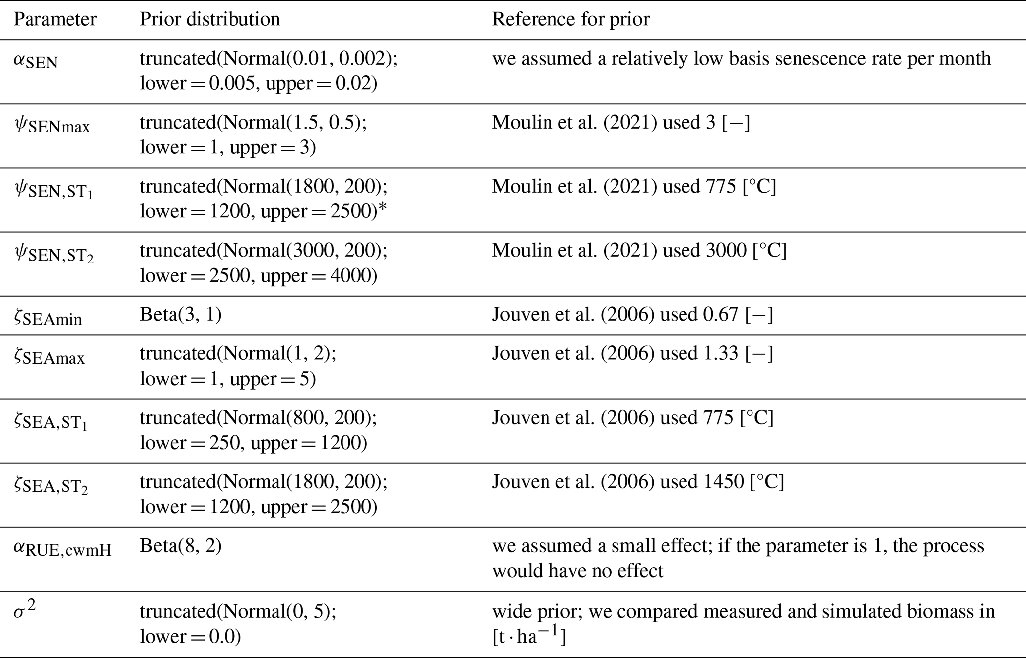
*Note that we assumed higher values for because we calibrated our model for lower altitudes compared to Moulin et al. (2021), as more heat is accumulated over the year before the senescence starts to increase in autumn.
Table F7Overview of experiments with location, year, and whether an experiment is used for calibration for the FAO dataset. If an experiment is not used for calibration, it is used for validation. We used only the subset of the experiments that were irrigated.
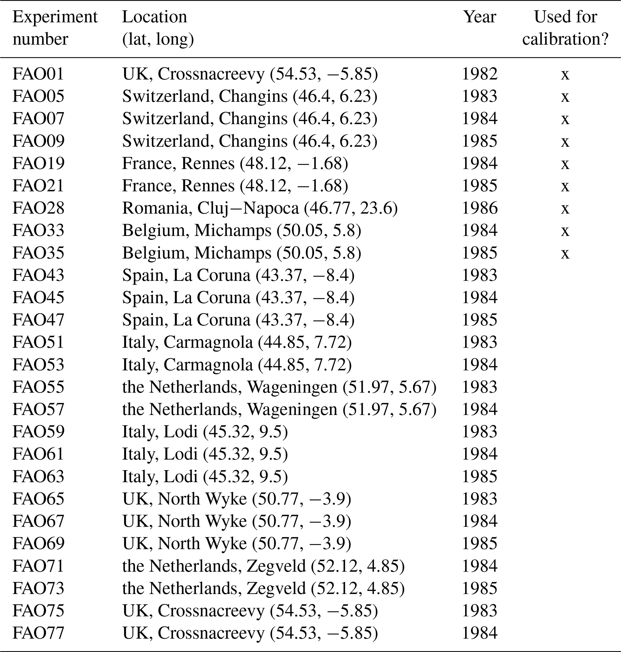
Table F8Prior distributions for calibration with the Biodiversity Exploratories dataset. The prior distributions for the parameters, which are rather theoretical, were set so that the simulated trajectories were close to the measured above-ground biomass and to the community-weighted mean traits.
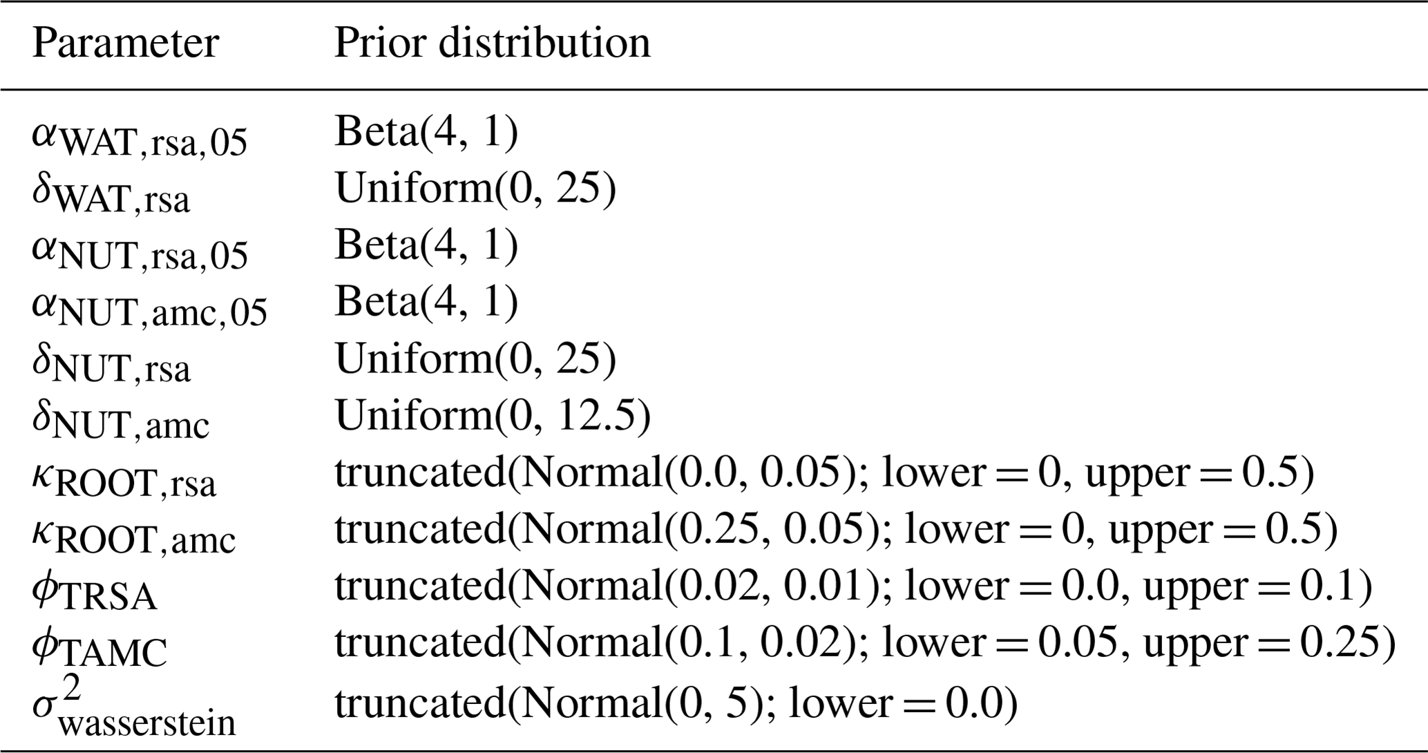
Table F9Overview of sites with location, dominant land use, and whether a site is used for calibration of the Biodiversity Exploratories dataset from the Schwäbische Alb region. If a site is not used for calibration, it is used for validation.
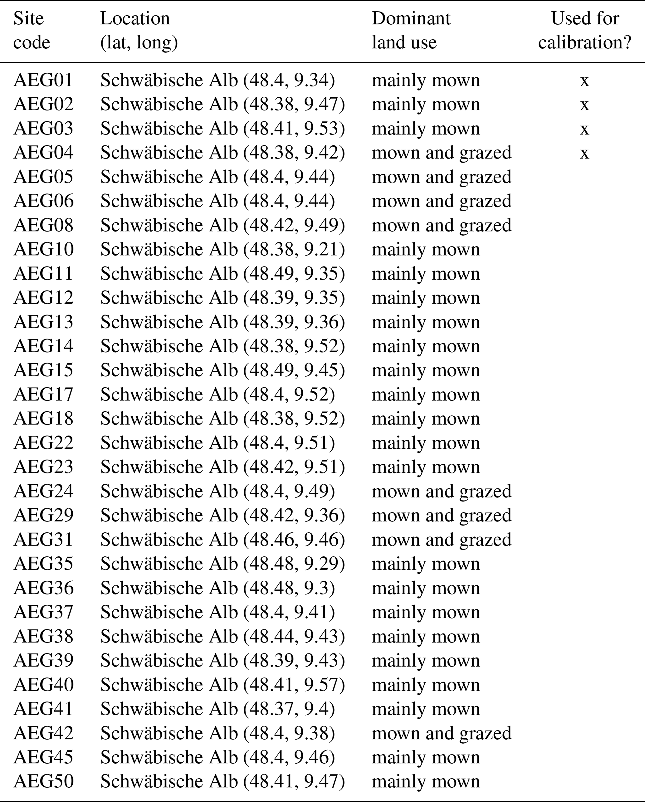
Table F10Overview of sites with location, dominant land use, and whether a site is used for calibration of the Biodiversity Exploratories dataset from the Hainich region. If a site is not used for calibration, it is used for validation.
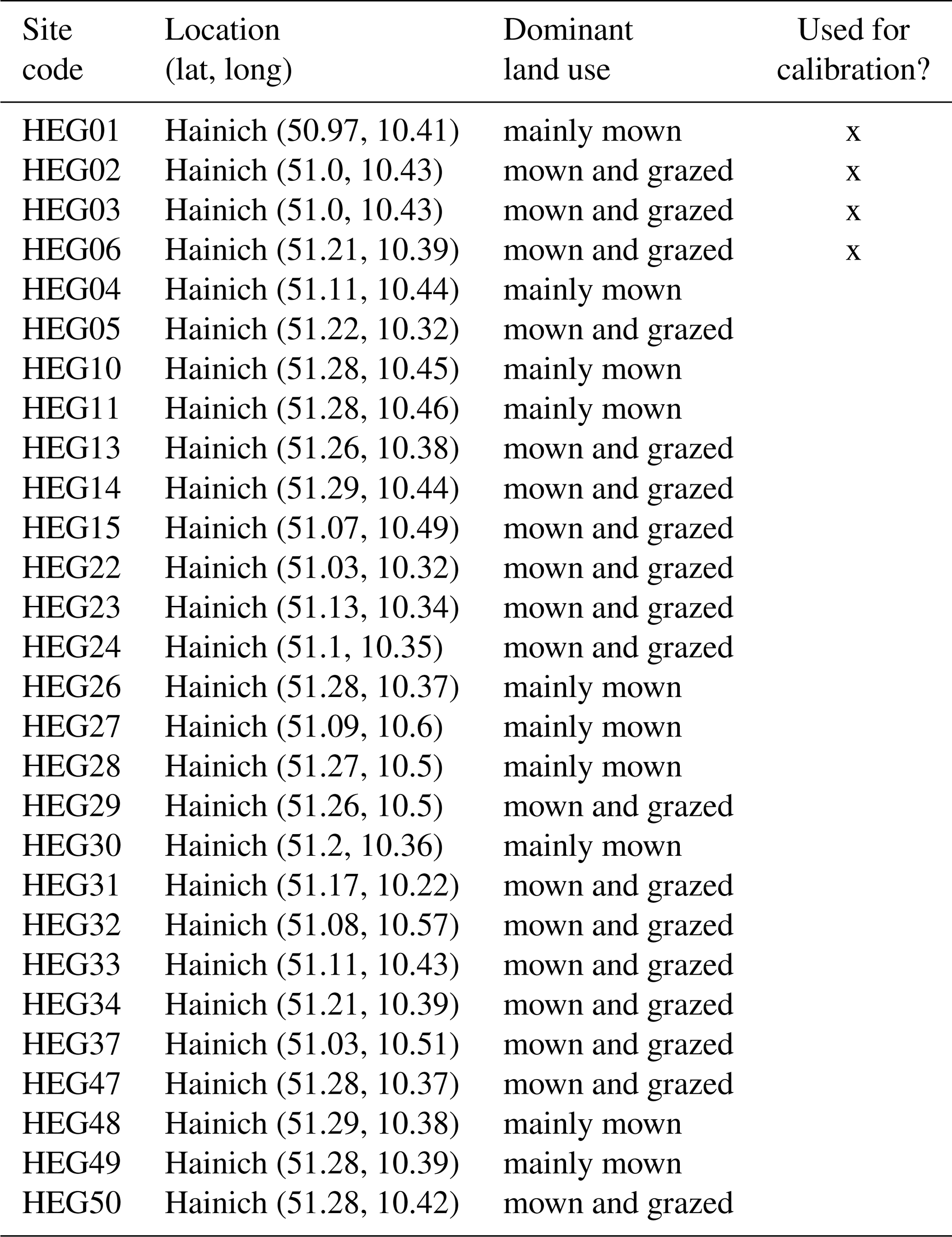
Table F11Overview of sites with location, dominant land use, and whether a site is used for calibration of the Biodiversity Exploratories dataset from the Schorfheide-Chorin region. If a site is not used for calibration, it is used for validation.
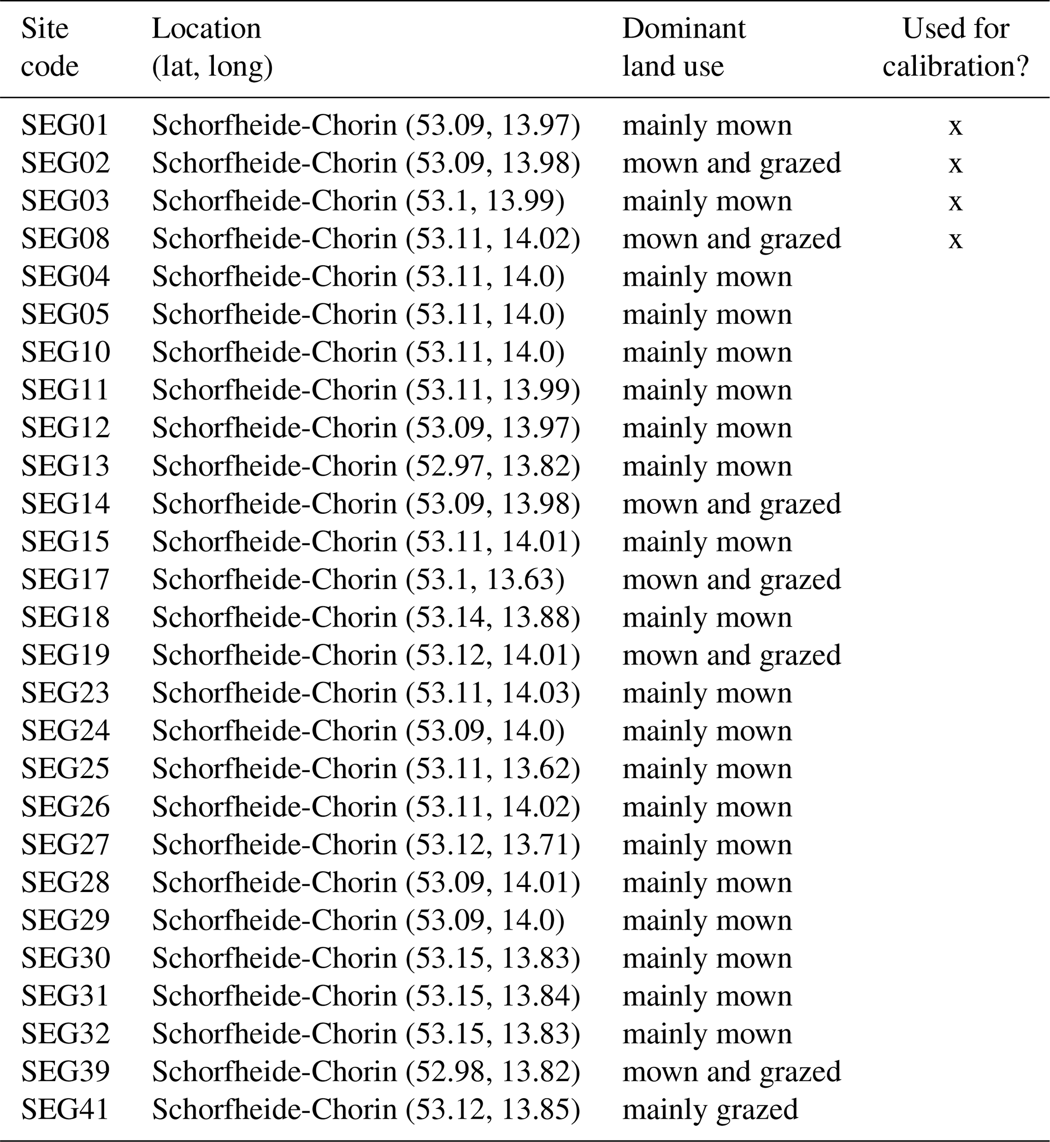
Table F12Sensitivity of above-ground biomass of Lolium perenne to changes in parameter values for all experiments in the FAO dataset. The default parameter values are listed in Table F4. We decreased (θ−) and increased (θ+) each parameter one at a time by 1 % (local sensitivity analysis). We calculated the output variable (denoted by Y) with one parameter decreased, one parameter increased, and the default parameters to calculate the following quotient: . We calculated the ratio for each time point and for all the experiments and took the overall average. All parameters not listed here have no influence on the biomass dynamic without soil water and nutrient growth limitation. The parameters are ordered from positive to small positive/negative effect to negative effect on the above-ground biomass.
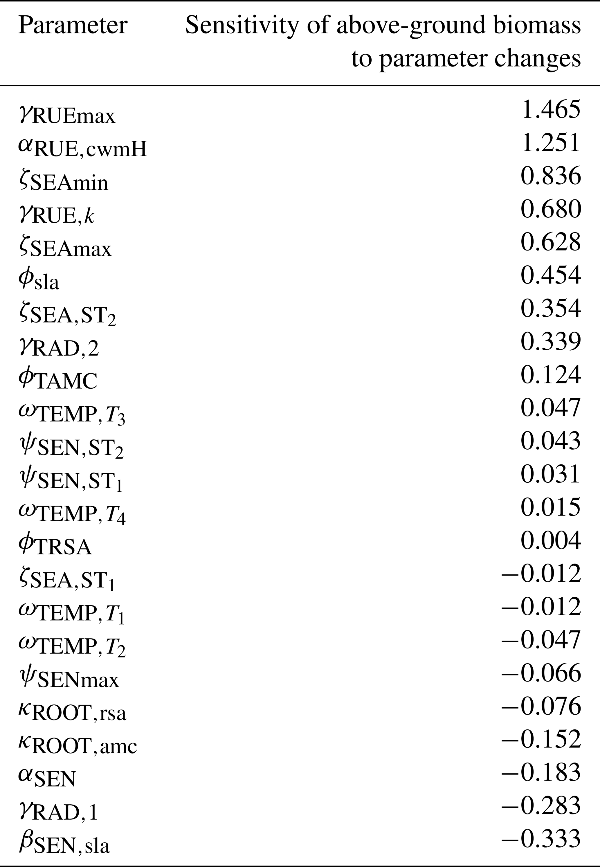
Table F13Sensitivity of the total above-ground biomass to changes in parameter values for all sites in the Biodiversity Exploratories dataset. The default parameter values are listed in Table F4. We decreased (θ−) and increased (θ+) each parameter one at a time by 1 % (local sensitivity analysis). We calculated the output variable (denoted by Y) with one parameter decreased, one parameter increased, and the default parameters to calculate the following quotient: . We calculated the ratio for each time point and for all the sites and took the overall average. The parameters are sorted into positive (left columns) and negative effect or almost no effect (right columns) on the total above-ground biomass.
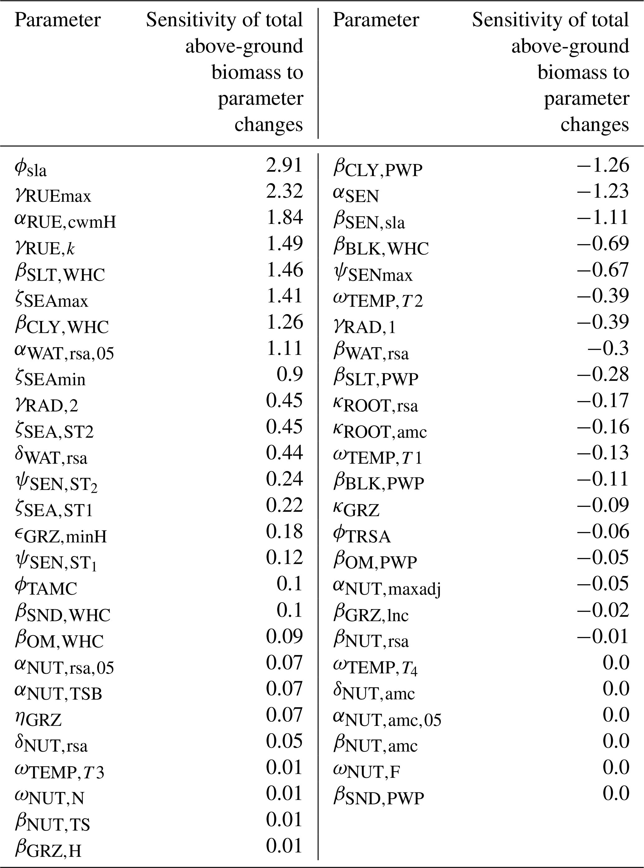
The model code, scripts for calibration, and raw and processed data for the calibration and validation can be found on Zenodo at https://doi.org/10.5281/zenodo.14011849 (Nößler, 2025). This work is partly based on data of the Biodiversity Exploratories programme (DFG Priority Programme 1374). These datasets are publicly available from the Biodiversity Exploratories Information System (https://doi.org/10.17616/R32P9Q, re3data.org, 2025) (with links to the specific datasets in the reference section) and are included in the Zenodo repository. The documentation of the model with installation instructions and tutorials can be found online at https://felixnoessler.github.io/GrasslandTraitSim.jl/ (last access: 8 September 2025).
Conceptualization: FN, FM, TM, and OB. Methodology: FN and TM. Software, formal analysis, visualization, and writing of the original draft: FN. Writing (review and editing): FN, BT, TM, FM, and OB. Supervision: FM, OB, BT, and TM.
The contact author has declared that none of the authors has any competing interests.
Publisher’s note: Copernicus Publications remains neutral with regard to jurisdictional claims made in the text, published maps, institutional affiliations, or any other geographical representation in this paper. While Copernicus Publications makes every effort to include appropriate place names, the final responsibility lies with the authors.
We would like to thank Florian Hartig for the discussion on calibration and Joana Bergmann for the discussion on below-ground plant traits. We thank the managers of the three exploratories Julia Bass, Miriam Teuscher, Franca Marian – and all former managers for their work in maintaining the plot and project infrastructure; Victoria Grießmeier for giving support through the central office; Andreas Ostrowski for managing the central database; and Markus Fischer, Eduard Linsenmair, Dominik Hessenmöller, Daniel Prati, Ingo Schöning, François Buscot, Ernst-Detlef Schulze, Wolfgang W. Weisser, and the late Elisabeth Kalko for their role in setting up the Biodiversity Exploratories project. We thank the administration of the Hainich National Park, the UNESCO Biosphere Reserve Swabian Alb, and the UNESCO Schorfheide-Chorin Biosphere Reserve as well as all landowners for the excellent collaboration. The work has been (partly) funded by the DFG Priority Programme 1374 “Biodiversity – Exploratories”. Field work permits were issued by the responsible state environmental offices of Baden-Württemberg, Thüringen, and Brandenburg.
The article processing charges for this open-access publication were covered by the Freie Universität Berlin.
This paper was edited by Roslyn Henry and reviewed by two anonymous referees.
Adler, P. B., Seabloom, E. W., Borer, E. T., Hillebrand, H., Hautier, Y., Hector, A., Harpole, W. S., O’Halloran, L. R., Grace, J. B., Anderson, T. M., Bakker, J. D., Biederman, L. A., Brown, C. S., Buckley, Y. M., Calabrese, L. B., Chu, C.-J., Cleland, E. E., Collins, S. L., Cottingham, K. L., Crawley, M. J., Damschen, E. I., Davies, K. F., DeCrappeo, N. M., Fay, P. A., Firn, J., Frater, P., Gasarch, E. I., Gruner, D. S., Hagenah, N., Hille Ris Lambers, J., Humphries, H., Jin, V. L., Kay, A. D., Kirkman, K. P., Klein, J. A., Knops, J. M. H., La Pierre, K. J., Lambrinos, J. G., Li, W., MacDougall, A. S., McCulley, R. L., Melbourne, B. A., Mitchell, C. E., Moore, J. L., Morgan, J. W., Mortensen, B., Orrock, J. L., Prober, S. M., Pyke, D. A., Risch, A. C., Schuetz, M., Smith, M. D., Stevens, C. J., Sullivan, L. L., Wang, G., Wragg, P. D., Wright, J. P., and Yang, L. H.: Productivity Is a Poor Predictor of Plant Species Richness, Science, 333, 1750–1753, https://doi.org/10.1126/science.1204498, 2011. a
Anten, N. P. R. and Hirose, T.: Interspecific differences in above-ground growth patterns result in spatial and temporal partitioning of light among species in a tall-grass meadow, J. Ecol., 87, 583–597, https://doi.org/10.1046/j.1365-2745.1999.00365.x, 1999. a
Archibald, S., Hempson, G. P., and Lehmann, C.: A unified framework for plant life‐history strategies shaped by fire and herbivory, New Phytol., 224, 1490–1503, https://doi.org/10.1111/nph.15986, 2019. a
Atkinson, J., Gallagher, R., Czyżewski, S., Kerr, M., Trepel, J., Buitenwerf, R., and Svenning, J.: Integrating functional traits into trophic rewilding science, J. Ecol., https://doi.org/10.1111/1365-2745.14307, 2024. a
Barber, S. A. and Silberbush, M.: Plant Root Morphology and Nutrient Uptake, in: Roots, Nutrient and Water Influx, and Plant Growth, ASA Special Publications, 49, 65–87, https://doi.org/10.2134/asaspecpub49.c4, 1984. a
Bergmann, J. and Rillig, M.: Fine root and mycorrhizal traits of 82 grassland species measured in a greenhouse experiment on sand, 2018, Biodiversity Exploratories Information System [data set], https://www.bexis.uni-jena.de/ddm/data/Showdata/26546?version=2 (last access: 8 September 2025), 2022. a
Bergmann, J., Weigelt, A., van der Plas, F., Laughlin, D. C., Kuyper, T. W., Guerrero-Ramirez, N., Valverde-Barrantes, O. J., Bruelheide, H., Freschet, G. T., Iversen, C. M., Kattge, J., McCormack, M. L., Meier, I. C., Rillig, M. C., Roumet, C., Semchenko, M., Sweeney, C. J., van Ruijven, J., York, L. M., and Mommer, L.: The fungal collaboration gradient dominates the root economics space in plants, Science Advances, 6, eaba3756, https://doi.org/10.1126/sciadv.aba3756, 2020. a, b, c
Bernton, E., Jacob, P. E., Gerber, M., and Robert, C. P.: On parameter estimation with the Wasserstein distance, Information and Inference: A Journal of the IMA, 8, 657–676, https://doi.org/10.1093/imaiai/iaz003, 2019. a
Bezanson, J., Edelman, A., Karpinski, S., and Shah, V. B.: Julia: A fresh approach to numerical computing, SIAM Rev. Soc. Ind. Appl. Math., 59, 65–98, https://doi.org/10.1137/141000671, 2017. a
Bonanomi, G., Giannino, F., Mazzoleni, S., and Setälä, H.: Negative Plant-Soil Feedback and Species Coexistence, Oikos, 111, 311–321, https://doi.org/10.1111/j.0030-1299.2005.13975.x, 2005. a
Bouman, B., Schapendonk, A., Stol, W., and van Kraalingen, D.: Description of the growth model LINGRA as implemented in CGMS, Quantitative Approaches in Systems Analysis, 7, 1–56, ISBN: 978-90-73384-47-7, 1996. a, b
Boval, M. and Sauvant, D.: Ingestive behaviour of grazing ruminants: Meta-analysis of the components linking bite mass to daily intake, Anim. Feed Sci. Tech., 278, 115014, https://doi.org/10.1016/j.anifeedsci.2021.115014, 2021. a
Buzhdygan, O. Y., Meyer, S. T., Weisser, W. W., Eisenhauer, N., Ebeling, A., Borrett, S. R., Buchmann, N., Cortois, R., De Deyn, G. B., de Kroon, H., Gleixner, G., Hertzog, L. R., Hines, J., Lange, M., Mommer, L., Ravenek, J., Scherber, C., Scherer-Lorenzen, M., Scheu, S., Schmid, B., Steinauer, K., Strecker, T., Tietjen, B., Vogel, A., Weigelt, A., and Petermann, J. S.: Biodiversity increases multitrophic energy use efficiency, flow and storage in grasslands, Nature Ecology & Evolution, 4, 393–405, https://doi.org/10.1038/s41559-020-1123-8, 2020. a
Caldwell, M. M.: Root Structure: The Considerable Cost of Belowground Function, in: Topics in Plant Population Biology, edited by: Solbrig, O. T., Jain, S., Johnson, G. B., and Raven, P. H., Macmillan Education UK, London, 408–427, https://doi.org/10.1007/978-1-349-04627-0_18, ISBN 978-1-349-04627-0, 1979. a
Canarini, A., Kaiser, C., Merchant, A., Richter, A., and Wanek, W.: Root Exudation of Primary Metabolites: Mechanisms and Their Roles in Plant Responses to Environmental Stimuli, Front. Plant Sci., 10, https://doi.org/10.3389/fpls.2019.00157, 2019. a
Chalmandrier, L., Hartig, F., Laughlin, D. C., Lischke, H., Pichler, M., Stouffer, D. B., and Pellissier, L.: Linking functional traits and demography to model species-rich communities, Nat. Commun., 12, https://doi.org/10.1038/s41467-021-22630-1, 2021. a, b, c, d, e, f, g, h, i, j
Chen, S., Wang, W., Xu, W., Wang, Y., Wan, H., Chen, D., Tang, Z., Tang, X., Zhou, G., Xie, Z., Zhou, D., Shangguan, Z., Huang, J., He, J.-S., Wang, Y., Sheng, J., Tang, L., Li, X., Dong, M., Wu, Y., Wang, Q., Wang, Z., Wu, J., Chapin, F. S., and Bai, Y.: Plant diversity enhances productivity and soil carbon storage, P. Natl. Acad. Sci. USA, 115, 4027–4032, https://doi.org/10.1073/pnas.1700298114, 2018. a
Clark, J. S., Carpenter, S. R., Barber, M., Collins, S., Dobson, A., Foley, J. A., Lodge, D. M., Pascual, M., Pielke Jr., R., and Pizer, W.: Ecological forecasts: an emerging imperative, Science, 293, 657–660, https://doi.org/10.1126/science.293.5530.657, 2001. a
Clerx, M., Robinson, M., Lambert, B., Lei, C. L., Ghosh, S., Mirams, G. R., and Gavaghan, D. J.: Probabilistic Inference on Noisy Time Series (PINTS), Journal of Open Research Software, 7, 23, https://doi.org/10.5334/jors.252, 2019. a, b
Confalonieri, R.: CoSMo: A simple approach for reproducing plant community dynamics using a single instance of generic crop simulators, Ecol. Model., 286, 1–10, https://doi.org/10.1016/j.ecolmodel.2014.04.019, 2014. a, b, c, d, e
Dee, L. E., Ferraro, P. J., Severen, C. N., Kimmel, K. A., Borer, E. T., Byrnes, J. E. K., Clark, A. T., Hautier, Y., Hector, A., Raynaud, X., Reich, P. B., Wright, A. J., Arnillas, C. A., Davies, K. F., MacDougall, A., Mori, A. S., Smith, M. D., Adler, P. B., Bakker, J. D., Brauman, K. A., Cowles, J., Komatsu, K., Knops, J. M. H., McCulley, R. L., Moore, J. L., Morgan, J. W., Ohlert, T., Power, S. A., Sullivan, L. L., Stevens, C., and Loreau, M.: Clarifying the effect of biodiversity on productivity in natural ecosystems with longitudinal data and methods for causal inference, Nat. Commun., 14, 2607, https://doi.org/10.1038/s41467-023-37194-5, 2023. a
Dickson, T. L., Mittelbach, G. G., Reynolds, H. L., and Gross, K. L.: Height and clonality traits determine plant community responses to fertilization, Ecology, 95, 2443–2452, https://doi.org/10.1890/13-1875.1, 2014. a
Díaz, S., Lavorel, S., McIntyre, S., Falczuk, V., Casanoves, F., Milchunas, D. G., Skarpe, C., Rusch, G., Sternberg, M., Noy-Meir, I., Landsberg, J., Zhang, W., Clark, H., and Campbell, B. D.: Plant trait responses to grazing – a global synthesis, Glob. Change Biol., 13, 313–341, https://doi.org/10.1111/j.1365-2486.2006.01288.x, 2007. a
DWD Climate Data Center: Calculated daily values for different characteristic elements of soil and crops, https://opendata.dwd.de/climate_environment/CDC/derived_germany/soil/daily/historical/ (last access: 3 September 2023), 2019. a
European Environment Agency, Kühn, E., Pettersson, L., Strien, A., Õunap, E., Warren, M., Settele, J., Švitra, G., Botham, M., Regan, E., Prokofev, I., Swaay, C., Stefanescu, C., Heliölä, J., Popov, S., Roth, T., Leopold, P., Verovnik, R., Fontaine, B., Musche, M., Julliard, R., Collins, S., Goloshchapova, S., Öberg, S., Cornish, N., Brereton, T., Titeux, N., Harpke, A., and Roy, D.: The European grassland butterfly indicator – 1990–2011, Publications Office of the European Union, https://doi.org/10.2800/89760, 2013. a
Eurostat: Main farm land use by NUTS 2 regions, https://doi.org/10.2908/ef_lus_main, 2020. a
Falster, D. S. and Westoby, M.: Plant height and evolutionary games, Trends Ecol. Evol., 18, 337–343, https://doi.org/10.1016/s0169-5347(03)00061-2, 2003. a
Fartmann, T.: Routledge Handbook of Insect Conservation, Chap. Insect Conservation in Grasslands, Routledge, ISBN 9781003285793, https://doi.org/10.4324/9781003285793, 2024. a
Fischer, M., Bossdorf, O., Gockel, S., Hänsel, F., Hemp, A., Hessenmöller, D., Korte, G., Nieschulze, J., Pfeiffer, S., Prati, D., Renner, S., Schöning, I., Schumacher, U., Wells, K., Buscot, F., Kalko, E. K. V., Linsenmair, K. E., Schulze, E.-D., and Weisser, W. W.: Implementing large-scale and long-term functional biodiversity research: The Biodiversity Exploratories, Basic Appl. Ecol., 11, 473–485, https://doi.org/10.1016/j.baae.2010.07.009, 2010. a
Fort, H.: On predicting species yields in multispecies communities: Quantifying the accuracy of the linear Lotka-Volterra generalized model, Ecol. Model., 387, 154–162, https://doi.org/10.1016/j.ecolmodel.2018.09.009, 2018. a
Funk, J. L., Larson, J. E., Ames, G. M., Butterfield, B. J., Cavender-Bares, J., Firn, J., Laughlin, D. C., Sutton-Grier, A. E., Williams, L., and Wright, J.: Revisiting the Holy Grail: using plant functional traits to understand ecological processes, Biol. Rev., 92, 1156–1173, https://doi.org/10.1111/brv.12275, 2017. a
Geijzendorffer, I. R., van der Werf, W., Bianchi, F. J. J. A., and Schulte, R. P. O.: Sustained dynamic transience in a Lotka-Volterra competition model system for grassland species, Ecol. Model., 222, 2817–2824, https://doi.org/10.1016/j.ecolmodel.2011.05.029, 2011. a
George, E., Marschner, H., and Jakobsen, I.: Role of Arbuscular Mycorrhizal Fungi in Uptake of Phosphorus and Nitrogen From Soil, CRC Cr. Rev. Biotechn., 15, 257–270, https://doi.org/10.3109/07388559509147412, 1995. a
Gillet, F.: Modelling vegetation dynamics in heterogeneous pasture-woodland landscapes, Ecol. Model., 217, 1–18, https://doi.org/10.1016/j.ecolmodel.2008.05.013, 2008. a
Goossens, E. P., Minden, V., Van Poucke, F., and Olde Venterink, H.: Negative plant-soil feedbacks disproportionally affect dominant plants, facilitating coexistence in plant communities, npj Biodiversity, 2, 27, https://doi.org/10.1038/s44185-023-00032-4, 2023. a
Gossner, M. M., Lewinsohn, T. M., Kahl, T., et al.: Land-use intensification causes multitrophic homogenization of grassland communities, Nature, 540, 266–269, https://doi.org/10.1038/nature20575, 2016. a
Gough, L., Gross, K. L., Cleland, E. E., Clark, C. M., Collins, S. L., Fargione, J. E., Pennings, S. C., and Suding, K. N.: Incorporating clonal growth form clarifies the role of plant height in response to nitrogen addition, Oecologia, 169, 1053–1062, https://doi.org/10.1007/s00442-012-2264-5, 2012. a, b
Griffin‐Nolan, R. J., Blumenthal, D. M., Collins, S. L., Farkas, T. E., Hoffman, A. M., Mueller, K. E., Ocheltree, T. W., Smith, M. D., Whitney, K. D., and Knapp, A. K.: Shifts in plant functional composition following long‐term drought in grasslands, J. Ecol., 107, 2133–2148, https://doi.org/10.1111/1365-2745.13252, 2019. a
Grime, J. P.: Evidence for the Existence of Three Primary Strategies in Plants and Its Relevance to Ecological and Evolutionary Theory, The American Naturalist, 111, 1169–1194, https://doi.org/10.1086/283244, 1977. a
Gross, K. L. and Mittelbach, G. G.: Negative effects of fertilization on grassland species richness are stronger when tall clonal species are present, Folia Geobot., 52, 401–409, https://doi.org/10.1007/s12224-017-9300-5, 2017. a
Gubsch, M., Buchmann, N., Schmid, B., Schulze, E.-D., Lipowsky, A., and Roscher, C.: Differential effects of plant diversity on functional trait variation of grass species, Ann. Bot., 107, 157–169, https://doi.org/10.1093/aob/mcq220, 2010. a
Gupta, S. C. and Larson, W. E.: Estimating soil water retention characteristics from particle size distribution, organic matter percent, and bulk density, Water Resour. Res., 15, 1633–1635, https://doi.org/10.1029/WR015i006p01633, 1979. a, b, c, d, e, f, g
Haario, H., Saksman, E., and Tamminen, J.: An Adaptive Metropolis Algorithm, Bernoulli, 7, 223–242, https://doi.org/10.2307/3318737, 2001. a
Heger, T.: Light availability experienced in the field affects ability of following generations to respond to shading in an annual grassland plant, J. Ecol., 104, 1432–1440, https://doi.org/10.1111/1365-2745.12607, 2016. a
Hejcman, M., Klaudisová, M., Schellberg, J., and Honsová, D.: The Rengen Grassland Experiment: Plant species composition after 64 years of fertilizer application, Agr. Ecosyst. Environ., 122, 259–266, https://doi.org/10.1016/j.agee.2006.12.036, 2007. a
Hejcman, M., Hejcmanová, P., Pavlů, V., and Beneš, J.: Origin and history of grasslands in Central Europe – a review, Grass Forage Sci., 68, 345–363, https://doi.org/10.1111/gfs.12066, 2013. a
Herold, N., Schöning, I., and Schrumpf, M.: Soil Survey 2008 Subplot Description, Biodiversity Exploratories Information System [data set], https://www.bexis.uni-jena.de/ddm/data/Showdata/4761?version=3 (last access: 8 September 2025), 2021. a
Hilpold, A., Seeber, J., Fontana, V., Niedrist, G., Rief, A., Steinwandter, M., Tasser, E., and Tappeiner, U.: Decline of rare and specialist species across multiple taxonomic groups after grassland intensification and abandonment, Biodivers. Conserv., 27, 3729–3744, https://doi.org/10.1007/s10531-018-1623-x, 2018. a
Hinderling, J. and Keller, S.: Vegetation records for grassland EPs, 2008 – 2022, Biodiversity Exploratories Information System [data set], https://www.bexis.uni-jena.de/ddm/data/Showdata/31389?version=7 (last access: 8 September 2025), 2023. a
Hinderling, J., Penone, C., Prati, D., Bolliger, R., Schäfer, D., Boch, S., and Schmitt, B.: Biomass data for grassland EPs, 2009–2023, Biodiversity Exploratories Information System [data set], https://www.bexis.uni-jena.de/ddm/data/Showdata/31581?version=5 (last access: 8 September 2025), 2024. a
Hirata, M., Kunieda, E., and Tobisa, M.: Short-term ingestive behaviour of cattle grazing tropical stoloniferous grasses with contrasting growth forms, J. Agr. Sci., 148, 615–624, https://doi.org/10.1017/S0021859610000353, 2010. a, b
Hodgson, J., Clark, D., and Mitchell, R.: Foraging Behavior in Grazing Animals and Its Impact on Plant Communities, in: Forage Quality, Evaluation, and Utilization, John Wiley & Sons, Ltd., 796–827, https://doi.org/10.2134/1994.foragequality.c19, 1994. a
Jäger, E. J., Müller, F., Ritz, C., Welk, E., and Wesche, K. (Eds.): Rothmaler – Exkursionsflora von Deutschland, Gefäßpflanzen: Atlasband, Springer Berlin Heidelberg, ISBN 9783662497104, https://doi.org/10.1007/978-3-662-49710-4, 2017. a
Jeltsch, F., Moloney, K. A., Schurr, F. M., Köchy, M., and Schwager, M.: The state of plant population modelling in light of environmental change, Perspectives in Plant Ecology, Evolution and Systematics, 9, 171–189, https://doi.org/10.1016/j.ppees.2007.11.004, 2008. a, b
Jiang, Y., Li, Y., Nie, G., and Liu, H.: Leaf and Root Growth, Carbon and Nitrogen Contents, and Gene Expression of Perennial Ryegrass to Different Nitrogen Supplies, J. Am. Soc. Hortic. Sci., 141, 555–562, https://doi.org/10.21273/JASHS03883-16, 2016. a
Johnstone, R. H., Chang, E. T., Bardenet, R., de Boer, T. P., Gavaghan, D. J., Pathmanathan, P., Clayton, R. H., and Mirams, G. R.: Uncertainty and variability in models of the cardiac action potential: Can we build trustworthy models?, J. Mol. Cell. Cardiol., 96, 49–62, https://doi.org/10.1016/j.yjmcc.2015.11.018, 2016. a
Jouven, M., Carrère, P., and Baumont, R.: Model predicting dynamics of biomass, structure and digestibility of herbage in managed permanent pastures. 1. Model description, Grass Forage Sci., 61, 112–124, https://doi.org/10.1111/j.1365-2494.2006.00515.x, 2006. a, b, c, d, e, f, g, h, i, j, k, l, m, n, o, p, q, r
Kattge, J., Bönisch, G., Díaz, S., et al.: TRY plant trait database – enhanced coverage and open access, Glob. Change Biol., 26, 119–188, https://doi.org/10.1111/gcb.14904, 2020. a, b
Kipling, R. P., Virkajärvi, P., Breitsameter, L., Curnel, Y., De Swaef, T., Gustavsson, A.-M., Hennart, S., Höglind, M., Järvenranta, K., Minet, J., Nendel, C., Persson, T., Picon-Cochard, C., Rolinski, S., Sandars, D. L., Scollan, N. D., Sebek, L., Seddaiu, G., Topp, C. F. E., Twardy, S., Van Middelkoop, J., Wu, L., and Bellocchi, G.: Key challenges and priorities for modelling European grasslands under climate change, Sci. Total Environ., 566-567, 851–864, https://doi.org/10.1016/j.scitotenv.2016.05.144, 2016. a
Klimešová, J., Latzel, V., de Bello, F., and van Groenendael, J. M.: Plant functional traits in studies of vegetation changes in response to grazing and mowing: towards a use of more specific traits, Preslia, 80, 245–253, 2008. a
Konvalinková, T., Püschel, D., Řezáčová, V., Gryndlerová, H., and Jansa, J.: Carbon flow from plant to arbuscular mycorrhizal fungi is reduced under phosphorus fertilization, Plant and Soil, 419, 319–333, https://doi.org/10.1007/s11104-017-3350-6, 2017. a
Kranstauber, B., Smolla, M., and Safi, K.: Similarity in spatial utilization distributions measured by the earth mover's distance, Methods Ecol. Evol., 8, 155–160, https://doi.org/10.1111/2041-210X.12649, 2017. a
Kunrath, T. R., Nunes, P. A. d. A., de Souza Filho, W., Cadenazzi, M., Bremm, C., Martins, A. P., and Carvalho, P. C. d. F.: Sward height determines pasture production and animal performance in a long-term soybean-beef cattle integrated system, Agr. Syst., 177, 102716, https://doi.org/10.1016/j.agsy.2019.102716, 2020. a
Lacasa, J., Hefley, T. J., Otegui, M. E., and Ciampitti, I. A.: A practical guide to estimating the light extinction coefficient with nonlinear models – a case study on maize, Plant Methods, 17, 60, https://doi.org/10.1186/s13007-021-00753-2, 2021. a, b
Lazzarotto, P., Calanca, P., and Fuhrer, J.: (2009). Dynamics of grass–clover mixtures – An analysis of the response to management with the PROductive GRASsland Simulator (PROGRASS), Ecol. Model., 220, 703–724, https://doi.org/10.1016/j.ecolmodel.2008.11.023, 2009. a, b
Liu, F. and Stützel, H.: Biomass partitioning, specific leaf area, and water use efficiency of vegetable amaranth (Amaranthus spp.) in response to drought stress, Sci. Hortic., 102, 15–27, https://doi.org/10.1016/j.scienta.2003.11.014, 2004. a
Liu, X., Parker, I. M., Gilbert, G. S., Lu, Y., Xiao, Y., Zhang, L., Huang, M., Cheng, Y., Zhang, Z., and Zhou, S.: Coexistence is stabilized by conspecific negative density dependence via fungal pathogens more than oomycete pathogens, Ecology, 103, https://doi.org/10.1002/ecy.3841, 2022. a
Long, S. P., Humphries, S., and Falkowski, P. G.: Photoinhibition of Photosynthesis in Nature, Annu. Rev. Plant Phys., 45, 633–662, https://doi.org/10.1146/annurev.pp.45.060194.003221, 1994. a
Lopez, G., Ahmadi, S. H., Amelung, W., Athmann, M., Ewert, F., Gaiser, T., Gocke, M. I., Kautz, T., Postma, J., Rachmilevitch, S., Schaaf, G., Schnepf, A., Stoschus, A., Watt, M., Yu, P., and Seidel, S. J.: Nutrient deficiency effects on root architecture and root-to-shoot ratio in arable crops, Front. Plant Sci., 13, https://doi.org/10.3389/fpls.2022.1067498, 2023. a
Luo, W., Ishii, N. I., Muraina, T. O., Song, L., Te, N., Griffin-Nolan, R. J., Slette, I. J., Ross, S. R. P. J., Sasaki, T., Rudgers, J. A., Smith, M. D., Knapp, A. K., and Collins, S. L.: Extreme Drought Increases the Temporal Variability of Grassland Productivity by Suppressing Dominant Grasses, Ecol. Lett., 28, e70127, https://doi.org/10.1111/ele.70127, 2025. a
Luo, Y., Weng, E., Wu, X., Gao, C., Zhou, X., and Zhang, L.: Parameter Identifiability, Constraint, and Equifinality in Data Assimilation with Ecosystem Models, Ecol. Appl., 19, 571–574, https://doi.org/10.1890/08-0561.1, 2009. a
Marschner, H. and Dell, B.: Nutrient uptake in mycorrhizal symbiosis, Plant Soil, 159, 89–102, https://doi.org/10.1007/bf00000098, 1994. a
May, F., Grimm, V., and Jeltsch, F.: Reversed effects of grazing on plant diversity: the role of below‐ground competition and size symmetry, Oikos, 118, 1830–1843, https://doi.org/10.1111/j.1600-0706.2009.17724.x, 2009. a, b, c, d
Meurer, K. H. E., Bolinder, M. A., Andrén, O., Hansson, A.-C., Pettersson, R., and Kätterer, T.: Shoot and root production in mixed grass ley under daily fertilization and irrigation: validating the N productivity concept under field conditions, Nutr. Cycl. Agroecosys., 115, 85–99, https://doi.org/10.1007/s10705-019-10006-3, 2019. a
Monsi, M.: Über den Lichtfaktor in den Pflanzengesellschaften und seine Bedeutung fur die Stoffproduktion, Jap. J. Bot., 14, 22–52, 1953. a
Monsi, M. and Saeki, T.: On the Factor Light in Plant Communities and its Importance for Matter Production, Ann. Bot., 95, 549–567, https://doi.org/10.1093/aob/mci052, 2005. a, b, c
Monteith, J. L.: Solar Radiation and Productivity in Tropical Ecosystems, J. Appl. Ecol., 9, 747–766, https://doi.org/10.2307/2401901, 1972. a
Moulin, T., Perasso, A., Calanca, P., and Gillet, F.: DynaGraM: A process-based model to simulate multi-species plant community dynamics in managed grasslands, Ecol. Model., 439, 109345, https://doi.org/10.1016/j.ecolmodel.2020.109345, 2021. a, b, c, d, e, f, g, h, i, j, k, l, m, n, o, p, q, r, s, t, u, v, w, x, y, z, aa, ab, ac, ad, ae, af, ag
Nagy, S.: Grasslands as a bird habitat, in: Grasslands in Europe: Of High Nature Value, KNNV Publishing, 35–41, ISBN 9789004278103, https://doi.org/10.1163/9789004278103_005, 2009. a
Nößler, F.: Supplementary material (empirical data for calibration and validation, model code, analysis scripts): A trait-based model to describe plant community dynamics in managed grasslands (GrasslandTraitSim.jl v1.0.0), Zenodo [code], https://doi.org/10.5281/zenodo.14011849, 2025. a
Onoda, Y., Wright, I. J., Evans, J. R., Hikosaka, K., Kitajima, K., Niinemets, Ü., Poorter, H., Tosens, T., and Westoby, M.: Physiological and structural tradeoffs underlying the leaf economics spectrum, New Phytol., 214, 1447–1463, https://doi.org/10.1111/nph.14496, 2017. a
Pakeman, R. J., Garnier, E., Lavorel, S., Ansquer, P., Castro, H., Cruz, P., Doležal, J., Eriksson, O., Freitas, H., Golodets, C., Kigel, J., Kleyer, M., Lepš, J., Meier, T., Papadimitriou, M., Papanastasis, V. P., Quested, H., Quétier, F., Rusch, G., Sternberg, M., Theau, J.-P., Thébault, A., and Vile, D.: Impact of abundance weighting on the response of seed traits to climate and land use, J. Ecol., 96, 355–366, https://doi.org/10.1111/j.1365-2745.2007.01336.x, 2008. a
Pärtel, M., Bruun, H., and Sammul, M.: Biodiversity in temperate European grasslands: origin and conservation, in: Integrating efficient grassland farming and biodiversity: Proceedings of the 13th international occasional symposium of the European grassland federation, Vol. 10 of Grassland Science in Europe, 1–14, ISBN: 9985-9611-3-7, 2005. a
Parton, W.: The CENTURY model, in: Evaluation of soil organic matter models: Using existing long-term datasets, Springer, 283–291, https://doi.org/10.1007/978-3-642-61094-3_23, 1996. a
Parton, W. J., Hartman, M., Ojima, D., and Schimel, D.: DAYCENT and its land surface submodel: description and testing, Global Planet. Change, 19, 35–48, https://doi.org/10.1016/S0921-8181(98)00040-X, 1998. a
Pauler, C. M., Isselstein, J., Suter, M., Berard, J., Braunbeck, T., and Schneider, M. K.: Choosy grazers: Influence of plant traits on forage selection by three cattle breeds, Funct. Ecol., 34, 980–992, https://doi.org/10.1111/1365-2435.13542, 2020. a
Pei, Y., Dong, J., Zhang, Y., Yuan, W., Doughty, R., Yang, J., Zhou, D., Zhang, L., and Xiao, X.: Evolution of light use efficiency models: Improvement, uncertainties, and implications, Agr. Forest Meteorol., 317, 108905, https://doi.org/10.1016/j.agrformet.2022.108905, 2022. a
Petermann, J. S. and Buzhdygan, O. Y.: Grassland biodiversity, Curr. Biol., 31, R1195–R1201, https://doi.org/10.1016/j.cub.2021.06.060, 2021. a, b
Piseddu, F., Bellocchi, G., and Picon-Cochard, C.: Mowing and warming effects on grassland species richness and harvested biomass: meta-analyses, Agron. Sustain. Dev., 41, https://doi.org/10.1007/s13593-021-00722-y, 2021. a
Piseddu, F., Martin, R., Movedi, E., Louault, F., Confalonieri, R., and Bellocchi, G.: Simulation of Multi-Species Plant Communities in Perturbed and Nutrient-Limited Grasslands: Development of the Growth Model ModVege, Agronomy, 12, https://doi.org/10.3390/agronomy12102468, 2022. a, b, c, d
Potts, J. R., Auger-Méthé, M., Mokross, K., and Lewis, M. A.: A generalized residual technique for analysing complex movement models using earth mover's distance, Methods Ecol. Evol., 5, 1012–1022, https://doi.org/10.1111/2041-210X.12253, 2014. a
Prati, D., Goßner, M., and Neff, F.: Leaf traits of most abundant plant species from all EPs, 2017/2018, Biodiversity Exploratories Information System [data set], https://www.bexis.uni-jena.de/ddm/data/Showdata/24807?version=2 (last access: 8 September 2025), 2021. a
Prieto, I., Roumet, C., Cardinael, R., Dupraz, C., Jourdan, C., Kim, J. H., Maeght, J. L., Mao, Z., Pierret, A., Portillo, N., Roupsard, O., Thammahacksa, C., and Stokes, A.: Root functional parameters along a land-use gradient: evidence of a community-level economics spectrum, J. Ecol., 103, 361–373, https://doi.org/10.1111/1365-2745.12351, 2015. a
Pulungan, M. A., Suzuki, S., Gavina, M. K. A., Tubay, J. M., Ito, H., Nii, M., Ichinose, G., Okabe, T., Ishida, A., Shiyomi, M., Togashi, T., Yoshimura, J., and Morita, S.: Grazing enhances species diversity in grassland communities, Sci. Rep., 9, https://doi.org/10.1038/s41598-019-47635-1, 2019. a
R Core Team: R: A Language and Environment for Statistical Computing, R Foundation for Statistical Computing, Vienna, Austria, https://www.R-project.org/ (last access: 1 October 2024), 2024. a
re3data.org: Biodiversity Exploratories Information System; re3data.org - Registry of Research Data Repositories [data set], https://doi.org/10.17616/R32P9Q, last access: 8 September 2025. a
Reich, P. B.: The world-wide “fast–slow” plant economics spectrum: a traits manifesto, J. Ecol., 102, 275–301, 2014. a
Reich, P. B., Walters, M. B., and Ellsworth, D. S.: Leaf Life-Span in Relation to Leaf, Plant, and Stand Characteristics among Diverse Ecosystems, Ecol. Monogr., 62, 365–392, https://doi.org/10.2307/2937116, 1992. a, b
Riedo, M., Grub, A., Rosset, M., and Fuhrer, J.: A pasture simulation model for dry matter production, and fluxes of carbon, nitrogen, water and energy, Ecol. Model., 105, 141–183, https://doi.org/10.1016/S0304-3800(97)00110-5, 1998. a, b, c
Rolinski, S., Müller, C., Heinke, J., Weindl, I., Biewald, A., Bodirsky, B. L., Bondeau, A., Boons-Prins, E. R., Bouwman, A. F., Leffelaar, P. A., te Roller, J. A., Schaphoff, S., and Thonicke, K.: Modeling vegetation and carbon dynamics of managed grasslands at the global scale with LPJmL 3.6, Geosci. Model Dev., 11, 429–451, https://doi.org/10.5194/gmd-11-429-2018, 2018. a, b
Rubner, Y., Tomasi, C., and Guibas, L. J.: The Earth Mover's Distance as a Metric for Image Retrieval, Int. J. Comput. Vision, 40, 99–121, https://doi.org/10.1023/a:1026543900054, 2000. a, b
Schapendonk, A. H. C. M., Stol, W., van Kraalingen, D. W. G., and Bouman, B. A. M.: LINGRA, a sink/source model to simulate grassland productivity in Europe, Eur. J. Agron., 9, 87–100, https://doi.org/10.1016/S1161-0301(98)00027-6, 1998. a, b, c, d, e, f, g, h, i, j, k, l, m, n, o, p, q, r
Schils, R. L. M., Newell Price, P., Klaus, V., Tonn, B., Hejduk, S., Stypinski, P., Hiron, M., Fernández, P., Ravetto Enri, S., Lellei-Kovács, E., Annett, N., Markovic, B., Lively, F., Ten Berge, H., Smith, K., Forster-Brown, C., Jones, M., Buchmann, N., Janicka, M., Fernandez, J., Rankin, J., McConnell, D., Aubry, A., and Korevaar, H.: European permanent grasslands mainly threatened by abandonment, heat and drought, and conversion to temporary grassland, Grassland Science in Europe, 25, 553–555, https://doi.org/10.3929/ETHZ-B-000448642, 2020. a, b
Schroeder-Georgi, T., Wirth, C., Nadrowski, K., Meyer, S. T., Mommer, L., and Weigelt, A.: From pots to plots: hierarchical trait-based prediction of plant performance in a mesic grassland, J. Ecol., 104, 206–218, https://doi.org/10.1111/1365-2745.12489, 2016. a
Schwinning, S. and Weiner, J.: Mechanisms determining the degree of size asymmetry in competition among plants, Oecologia, 113, 447–455, https://doi.org/10.1007/s004420050397, 1998. a
Schöning, I.: Soil carbon and nitrogen concentrations – soil sampling campaign 2021, all experimental plots (EPs), 0–10 cm, Biodiversity Exploratories Information System [data set], https://www.bexis.uni-jena.de/ddm/data/Showdata/31210?version=13 (last access: 8 September 2025), 2023. a
Schöning, I., Klötzing, T., Apostolakis, A., Trumbore, S., and Schrumpf, M.: MinSoil 2017 – Soil Carbon and Nitrogen Concentrations, Biodiversity Exploratories Information System [data set], https://www.bexis.uni-jena.de/ddm/data/Showdata/23846?version=10 (last access: 8 September 2025), 2021a. a
Schöning, I., Solly, E., Klötzing, T., Trumbore, S., and Schrumpf, M.: MinSoil 2011 – Soil Carbon and Nitrogen Concentrations, Biodiversity Exploratories Information System [data set], https://www.bexis.uni-jena.de/ddm/data/Showdata/14446?version=19 (last access: 8 September 2025), 2021b. a, b
Schöning, I., Solly, E., Klötzing, T., Trumbore, S., and Schrumpf, M.: MinSoil 2011 – Soil Texture, Biodiversity Exploratories Information System [data set], https://www.bexis.uni-jena.de/ddm/data/Showdata/14686?version=10 (last access: 8 September 2025), 2021c. a
Schöning, I., Solly, E., Klötzing, T., Trumbore, S., and Schrumpf, M.: MinSoil 2011 – Soil Bulk Density and Carbon and Nitrogen stocks, Biodiversity Exploratories Information System [data set], https://www.bexis.uni-jena.de/ddm/data/Showdata/17086?version=4 (last access: 8 September 2025), 2021d. a
Schöning, I., Trumbore, S., Schrumpf, M., Klötzing, T., and Gan, H. Y.: MinSoil 2014 – Soil Carbon and Nitrogen Concentrations, Biodiversity Exploratories Information System [data set], https://www.bexis.uni-jena.de/ddm/data/Showdata/18787?version=6 (last access: 8 September 2025), 2021e. a
Siefert, A., Violle, C., Chalmandrier, L., et al.: A global meta-analysis of the relative extent of intraspecific trait variation in plant communities, Ecol. Lett., 18, 1406–1419, https://doi.org/10.1111/ele.12508, 2015. a
Siehoff, S., Lennartz, G., Heilburg, I. C., Roß-Nickoll, M., Ratte, H. T., and Preuss, T. G.: Process-based modeling of grassland dynamics built on ecological indicator values for land use, Ecol. Model., 222, 3854–3868, https://doi.org/10.1016/j.ecolmodel.2011.10.003, 2011. a, b, c, d
Silva, G. P., Fialho, C. A., Carvalho, L. R., Fonseca, L., Carvalho, P. C. F., Bremm, C., and Da Silva, S. C.: Sward structure and short-term herbage intake in Arachis pintoi cv. Belmonte subjected to varying intensities of grazing, J. Agr. Sci., 156, 92–99, https://doi.org/10.1017/S0021859617000855, 2018. a
Tälle, M., Deák, B., Poschlod, P., Valkó, O., Westerberg, L., and Milberg, P.: Grazing vs. mowing: A meta-analysis of biodiversity benefits for grassland management, Agr. Ecosyst. Environ., 222, 200–212, https://doi.org/10.1016/j.agee.2016.02.008, 2016. a
Taubert, F., Frank, K., and Huth, A.: A review of grassland models in the biofuel context, Ecol. Model., 245, 84–93, https://doi.org/10.1016/j.ecolmodel.2012.04.007, 2012. a, b, c, d, e, f, g, h, i
Taubert, F., Hetzer, J., Schmid, J. S., and Huth, A.: Confronting an individual-based simulation model with empirical community patterns of grasslands, PLOS ONE, 15, e0236546, https://doi.org/10.1371/journal.pone.0236546, 2020. a, b
Van Der Heijden, M. G. A., Martin, F. M., Selosse, M., and Sanders, I. R.: Mycorrhizal ecology and evolution: the past, the present, and the future, New Phytol., 205, 1406–1423, https://doi.org/10.1111/nph.13288, 2015. a
Van Oijen, M., Bellocchi, G., and Höglind, M.: Effects of Climate Change on Grassland Biodiversity and Productivity: The Need for a Diversity of Models, Agronomy, 8, 14, https://doi.org/10.3390/agronomy8020014, 2018. a
Van Oijen, M., Barcza, Z., Confalonieri, R., Korhonen, P., Kröel-Dulay, G., Lellei-Kovács, E., Louarn, G., Louault, F., Martin, R., Moulin, T., Movedi, E., Picon-Cochard, C., Rolinski, S., Viovy, N., Wirth, S. B., and Bellocchi, G.: Incorporating Biodiversity into Biogeochemistry Models to Improve Prediction of Ecosystem Services in Temperate Grasslands: Review and Roadmap, Agronomy, 10, 259, https://doi.org/10.3390/agronomy10020259, 2020. a, b
Vehtari, A., Gelman, A., Simpson, D., Carpenter, B., and Bürkner, P.-C.: Rank-normalization, folding, and localization: An improved R̂ for assessing convergence of MCMC (with discussion), Bayesian Anal., 16, 667–718, https://doi.org/10.1214/20-BA1221, 2021. a
Villani, C.: Optimal Transport – Old and New, Springer Berlin Heidelberg, ISBN 9783540710509, https://doi.org/10.1007/978-3-540-71050-9, 2009. a
Violle, C., Enquist, B. J., McGill, B. J., Jiang, L., Albert, C. H., Hulshof, C., Jung, V., and Messier, J.: The return of the variance: intraspecific variability in community ecology, Trends Ecol. Evol., 27, 244–252, https://doi.org/10.1016/j.tree.2011.11.014, 2012. a
Virtanen, P., Gommers, R., Oliphant, T. E., Haberland, M., Reddy, T., Cournapeau, D., Burovski, E., Peterson, P., Weckesser, W., Bright, J., van der Walt, S. J., Brett, M., Wilson, J., Millman, K. J., Mayorov, N., Nelson, A. R. J., Jones, E., Kern, R., Larson, E., Carey, C. J., Polat, İ., Feng, Y., Moore, E. W., VanderPlas, J., Laxalde, D., Perktold, J., Cimrman, R., Henriksen, I., Quintero, E. A., Harris, C. R., Archibald, A. M., Ribeiro, A. H., Pedregosa, F., van Mulbregt, P., and SciPy 1.0 Contributors: SciPy 1.0: Fundamental Algorithms for Scientific Computing in Python, Nat. Methods, 17, 261–272, https://doi.org/10.1038/s41592-019-0686-2, 2020. a
Vogt, J., Weisser, W., Ayasse, M., Fischer, M., Schumacher, U., Schreiber, C., Lauterbach, R., Franke, A., Ostrowski, A., Teuscher, M., and Pompe, S.: Grassland management parameter as input data for a computer model based on interview data of the Biodiversity Exploratories project, Biodiversity Exploratories Information System [data set], https://www.bexis.uni-jena.de/ddm/data/Showdata/31715?version=9 (last access: 8 September 2025), 2024. a
Wang, D.: MODIS/Terra+Aqua Photosynthetically Active Radiation Daily/3-Hour L3 Global 0.05Deg CMG V061, NASA EOSDIS Land Processes Distributed Active Archive Center [data set], https://doi.org/10.5067/MODIS/MCD18C2.061, 2021. a
Watson, D. J.: Comparative Physiological Studies on the Growth of Field Crops: I. Variation in Net Assimilation Rate and Leaf Area between Species and Varieties, and within and between Years, Ann. Bot., 11, 41–76, https://doi.org/10.1093/oxfordjournals.aob.a083148, 1947. a
Weiner, J.: Asymmetric competition in plant populations, Trends Ecol. Evol., 5, 360–364, https://doi.org/10.1016/0169-5347(90)90095-U, 1990. a
Went, F.: The effect of temperature on plant growth, Annu. Rev. Plant Physio., 4, 347–362, https://doi.org/10.1146/annurev.pp.04.060153.002023, 1953. a
Westoby, M., Falster, D. S., Moles, A. T., Vesk, P. A., and Wright, I. J.: Plant ecological strategies: some leading dimensions of variation between species, Annu. Rev. Ecol. Syst., 33, 125–159, https://doi.org/10.1146/annurev.ecolsys.33.010802.150452, 2002. a
Wilson, J. B., Peet, R. K., Dengler, J., and Pärtel, M.: Plant species richness: the world records, J. Veg. Sci., 23, 796–802, https://doi.org/10.1111/j.1654-1103.2012.01400.x, 2012. a
Wirth, S. B., Taubert, F., Tietjen, B., Müller, C., and Rolinski, S.: Do details matter? Disentangling the processes related to plant species interactions in two grassland models of different complexity, Ecol. Model., 460, 109737, https://doi.org/10.1016/j.ecolmodel.2021.109737, 2021. a
Wirth, S. B., Poyda, A., Taube, F., Tietjen, B., Müller, C., Thonicke, K., Linstädter, A., Behn, K., Schaphoff, S., von Bloh, W., and Rolinski, S.: Connecting competitor, stress-tolerator and ruderal (CSR) theory and Lund Potsdam Jena managed Land 5 (LPJmL 5) to assess the role of environmental conditions, management and functional diversity for grassland ecosystem functions, Biogeosciences, 21, 381–410, https://doi.org/10.5194/bg-21-381-2024, 2024. a, b, c, d
Wright, G. C., Hubick, K. T., Farquhar, G. D., and Rao, R. N.: Genetic and environmental variation in transpiration efficiency and its correlation with carbon isotope discrimination and specific leaf area in peanut, in: Stable isotopes and plant carbon-water relations, Elsevier, 247–267, https://doi.org/10.1016/B978-0-08-091801-3.50025-8, 1993. a
Wright, I. J., Reich, P. B., Westoby, M., Ackerly, D. D., Baruch, Z., Bongers, F., Cavender-Bares, J., Chapin, T., Cornelissen, J. H. C., Diemer, M., Flexas, J., Garnier, E., Groom, P. K., Gulias, J., Hikosaka, K., Lamont, B. B., Lee, T., Lee, W., Lusk, C., Midgley, J. J., Navas, M.-L., Niinemets, Ü., Oleksyn, J., Osada, N., Poorter, H., Poot, P., Prior, L., Pyankov, V. I., Roumet, C., Thomas, S. C., Tjoelker, M. G., Veneklaas, E. J., and Villar, R.: The worldwide leaf economics spectrum, Nature, 428, 821–827, https://doi.org/10.1038/nature02403, 2004. a, b, c
Wöllauer, S., Hänsel, F., Nauss, T., and Forteva, S.: Climate data – Time Series Web Interface, Biodiversity Exploratories Information System [data set], https://www.bexis.uni-jena.de/tcd/PublicClimateData/ (last access: 1 May 2025), 2023. a
- Abstract
- Introduction
- Description of the GrasslandTraitSim.jl model
- Calibration and validation of the model
- Discussion
- Conclusions
- Appendix A: Derivation of the species-specific water and nutrient growth reducers
- Appendix B: Technical details of the GrasslandTraitSim.jl model
- Appendix C: Detailed description and data preparation for the Biodiversity Exploratories dataset
- Appendix D: Calculating the distance between two community trait distributions
- Appendix E: Technical details on running the Markov chain Monte Carlo routine
- Appendix F: Supporting figures and tables
- Code and data availability
- Author contributions
- Competing interests
- Disclaimer
- Acknowledgements
- Financial support
- Review statement
- References