Aging and stress explain the earlier start of leaf senescence in trees in warmer years: translating the latest findings on senescence regulation into the DP3 model (v1.1)

Leaf senescence ends the growing season of deciduous trees, affecting the amount of atmospheric CO₂ sequestered by forests. Therefore, some climate models integrate projected leaf senescence dates to simulate the carbon cycle. Here, we developed a process-oriented model of leaf senescence (the “DP3 model”) by testing 34 formulations of the leaf development process based on the latest findings on the regulation of leaf aging and senescence. The period between leaf unfolding and leaf senescence was separated into the subsequent young, mature, and old leaf phases, with particular reactions to leaf aging and cold stress, photoperiod stress, and dry stress. The DP3 model simulates daily rates of aging and stress to predict dates of transition from young to mature to old leaf, senescence induction dates, and leaf senescence dates. This allows new hypotheses regarding the regulation of leaf senescence to be tested. For example, the DP3 model predicted an earlier onset of senescence in warmer conditions, likely due to earlier leaf unfolding (aging) and increased cold and dry stress in spring, together with longer-lasting senescence, likely due to the later accumulation of photoperiod stress relative to leaf development and decreased cold stress in summer and fall, which can be validated through experiments and in situ observations. The DP3 model and compared previous models were equally accurate but less accurate than the Null model (average senescence date observed in the calibration sample). This lower accuracy of the DP3 and compared models is likely due to noise in the visually observed leaf senescence data, which blurs the signal of the leaf senescence process, and to incorrect model formulations. The model errors were similarly affected by climate conditions and location among compared models (including the Null model) and varied mostly due to the leaf senescence data. Noisy leaf senescence data likely force the models to resort to the mean observation, impeding inferences from accuracy-based model comparisons about the leaf senescence process. This calls for revised observation protocols and methods that measure rather than estimate different senescence stages, such as senescence induction and 50 % of the leaves having changed color, e.g., based on greenness, involving digital cameras and automated image assessment.

1 Introduction

Leaf senescence involves several processes and regulation pathways, but the most important process is the degradation of chlorophyll and breakdown of chloroplasts to retrieve nutrients, especially nitrogen, and to mobilize them in new leaves in spring (Cooke and Weih, 2005; Keskitalo et al., 2005; Lim et al., 2007; Rogers, 2017). A side effect of this nutrient resorption is the change in leaf color from green to yellow, orange, or red (Keskitalo et al., 2005, but see Wheeler and Dietze, 2023). There have been many studies on how the timing of leaf coloring is influenced by climatic conditions (e.g., Bigler and Vitasse, 2021; Liu et al., 2018; Meier et al., 2021). As these studies usually used the term “leaf coloring” or “leaf senescence” to refer to a particular stage of leaf senescence, we use “leaf senescence” as a collective term for the stages when a given relative amount of leaves have changed color or have fallen, unless stated otherwise.

Leaf senescence marks the end of a process that has been better understood over the last 10 years, mainly thanks to studies in cell and molecular biology and in environmental sciences. These studies have shown that leaf senescence relates to leaf development state (e.g., Jan et al., 2019; Jibran et al., 2013; Lim et al., 2007). On the one hand, the development state of leaves depends on their age and thus on the time since leaf unfolding and the state of carbohydrate sinks (Jibran et al., 2013), which relates to photosynthetic activity and nutrient availability (Paul and Foyer, 2001). While earlier leaf unfolding was related to earlier leaf senescence (Fu et al., 2014, 2019), an intense discussion has started about the possibility of earlier leaf senescence due to increased photosynthetic activity (Kloos et al., 2024; Lu and Keenan, 2022; Marqués et al., 2023; Norby, 2021; Zohner et al., 2023). On the other hand, the development state of leaves is influenced by hormone levels (Addicott, 1968; Jan et al., 2019; Jibran et al., 2013; Lim et al., 2007), which are, among others, stimulated by environmental stress caused by cold (Kloos et al., 2024; Wang et al., 2022; Xie et al., 2015, 2018), drought (Bigler and Vitasse, 2021; Mariën et al., 2021; Tan et al., 2023; but see Kloos et al., 2024; Xie et al., 2015, 2018), heat (Bigler and Vitasse, 2021; Mariën et al., 2021; Tan et al., 2023; Xie et al., 2015, 2018), heavy rain (Kloos et al., 2024; Xie et al., 2015, 2018), short days (Addicott, 1968; Keskitalo et al., 2005; Singh et al., 2017; Tan et al., 2023; Wang et al., 2022), and lack of nutrients (Fu et al., 2019; Tan et al., 2023). In the early phase of leaf development (“young leaf”), senescence cannot be induced, whereas aging and stress induce it in later phases (“mature leaf” and “old leaf”) and regulate the rate of senescence (Fig. 1; Jan et al., 2019; Jibran et al., 2013; Lim et al., 2007; Paul and Foyer, 2001; Tan et al., 2023).

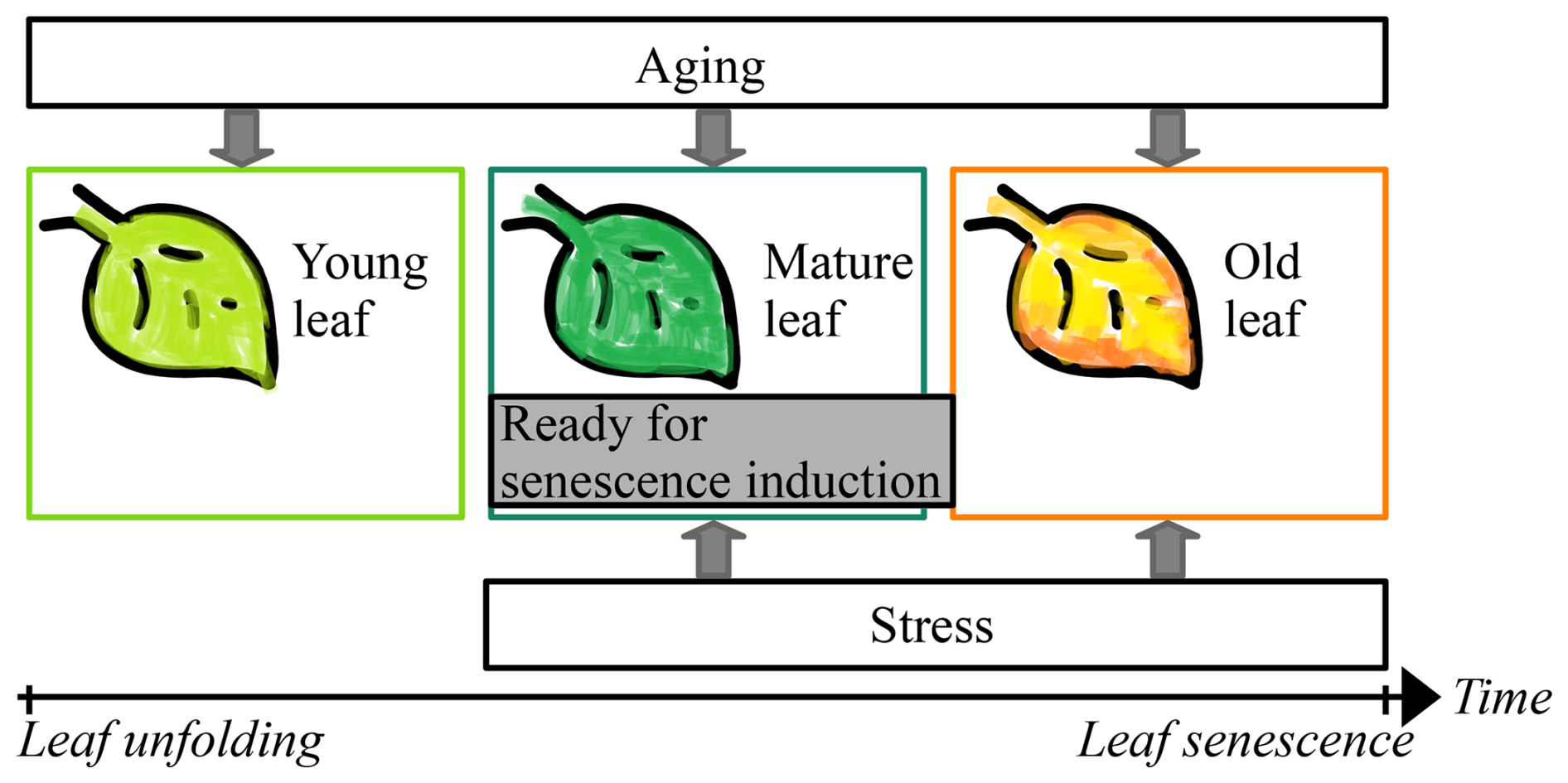
Figure 1 Leaf development. Starting with leaf unfolding, the young leaf develops first into a mature leaf and then into an old leaf. During the three phases of the young, mature, and old leaf, the leaf ages continuously. With the transition from young to mature leaf, the leaf becomes ready for senescence induction through environmental stress (e.g., cold days). If senescence is not induced through stress in the mature leaf, it certainly is through aging with the transition from mature to old leaf. Thus, senescence cannot be induced during the phase of the young leaf and the onset of senescence (i.e., the senescence induction date) depends on the time since leaf unfolding and on the environmental conditions since the transition from young to mature leaf. Adapted from Fig. 1 in Jibran et al. (2013).

As senescence induction depends on environmental conditions, leaf senescence of deciduous trees shifts as climate changes, which influences the timing and length of their growing season and thus affects the amount of CO₂ absorbed from the atmosphere (Meier et al., 2021; Menzel et al., 2020; Piao et al., 2019; but see Mariën et al., 2021). This links the feedback loop between atmospheric CO₂ concentration and climate to the feedback loop between climate and forests and more generally to terrestrial ecosystems (Luo, 2007; Richardson et al., 2013). Further, the amount of absorbed CO₂ relates to the amount of sugars available for tree growth, defense, and reproduction (Herms and Mattson, 1992; Tan et al., 2023). Therefore, accurate projections of leaf senescence dates under a changing climate are necessary for accurate forecasts of both climate change and future species composition of temperate forests.

Leaf senescence dates are often projected using process-oriented models. These models are usually based on the results of experiments testing the effect of various environmental cues that are translated mathematically (Chuine et al., 2013; Chuine and Régnière, 2017). Various process-oriented models of leaf senescence have been proposed over the last 20 years (Liu et al., 2020; Meier and Bigler, 2023). They generally formulate leaf senescence as a one-way process that starts shortly after summer solstice by accumulating a daily rate of senescence until a threshold is reached (but see Wheeler and Dietze, 2023). The daily rate is usually dependent on temperature and day length, and the threshold is either a constant or depends on leaf unfolding dates or on environmental conditions during the growing season (e.g., Delpierre et al., 2009; Keenan and Richardson, 2015; Liu et al., 2019; Zani et al., 2020).

Previous studies have shown that these leaf senescence models are heavily biased towards the mean of the calibration sample (Meier et al., 2023) and are less efficient relatively to leaf unfolding models (e.g., Liu et al., 2020; Meier and Bigler, 2023). However, it is not yet clear whether this is due to noisy phenological data and/or an incomplete process formulation.

The phenological data used to train leaf senescence models have often been recordings of visual observations, which cover long time periods and are species-specific (e.g., ongoing since 1951 in the Swiss phenology network, 2025). However, the observations are noisy due to different observers and small sample sizes. For leaf senescence, Liu et al. (2021) showed, e.g., that the observer bias was 15 d (days; median) and the sampling bias was 10 d (median) for 10 trees observed per population. These biases lead not only to noise between sites but also within sites when observers and samples change. Such changes can lead to sudden changes in the mean in the time series, as was found for some Swiss sites (Auchmann et al., 2018; Swiss phenology network, 2025). Moreover, the observation protocols may differ between the meteorological institutes and citizen-science-based networks that are responsible for the recording in the different European countries (Menzel, 2013).

Current models formulate leaf senescence as the result of an accumulated stress caused by cold and short days after summer solstice (Delpierre et al., 2009; Dufrêne et al., 2005; Keenan and Richardson, 2015; Lang et al., 2019; Liu et al., 2019; Zani et al., 2020). Two models further consider environmental conditions before summer solstice, either through temperature and precipitation during the growing season (Liu et al., 2019) or through photosynthetic activity during the growing season (Zani et al., 2020), while one model considers age through leaf unfolding dates (Keenan and Richardson, 2015). However, in these models, environmental conditions and age affect the amount of stress needed for leaf senescence rather than senescence induction. In other words, according to current models, senescence induction depends only on stress caused by cold and short days after summer solstice, which considerably contrasts with current knowledge (see above). None of the current models allows for senescence induction due to aging or stress before summer solstice. While two models consider stress that occurred before summer solstice, senescence is always induced after summer solstice. Finally, we are unaware if aging, stress caused by other than cold and short days, and different stress effects among the phases of leaf development have been tested, as none of the corresponding studies mentioned tested but discarded model formulations.

Here, we developed a new process-oriented model that predicts leaf senescence dates based on the latest knowledge of the physiological processes and drivers of leaf senescence. Leaf senescence was formulated through a leaf development process that starts at leaf unfolding and is driven by aging and various types of abiotic stress. We tested 34 model formulations of this process. Finally, the most accurate formulation was evaluated with a particular focus on the differences between the predicted and observed dates (i.e., “model errors”). We addressed the following research questions:

1. Which model formulation yields the most accurate predictions of leaf senescence dates?

2. How accurately does this model predict leaf senescence dates compared to previous models?

3. How do the model errors relate to the phenological data, climate, and site conditions?

2 Data and methods

2.1 Phenological data

The model was developed and evaluated with leaf phenology data of common beech (Fagus sylvatica L.), which was visually observed in Austria, Germany, Great Britain, and Switzerland between 1950 and 2022 (Fig. 2, Table 1, Sect. S1.1 in the Supplement; PEP725, 2024; Swiss phenology network, 2025; Templ et al., 2018). We used the phenological stages, with 50 % of the leaves having unfolded as well as 50 % and 100 % of the leaves having changed color or having fallen (hereafter referred to as “leaf unfolding” [LU], “leaf senescence₅₀” [LS₅₀], and “leaf senescence₁₀₀” [LS₁₀₀], respectively, corresponding to BBCH15, BBCH95, and BBCH97 according to Meier, 2018). The LS₁₀₀ data were recorded in Austria and Great Britain only.

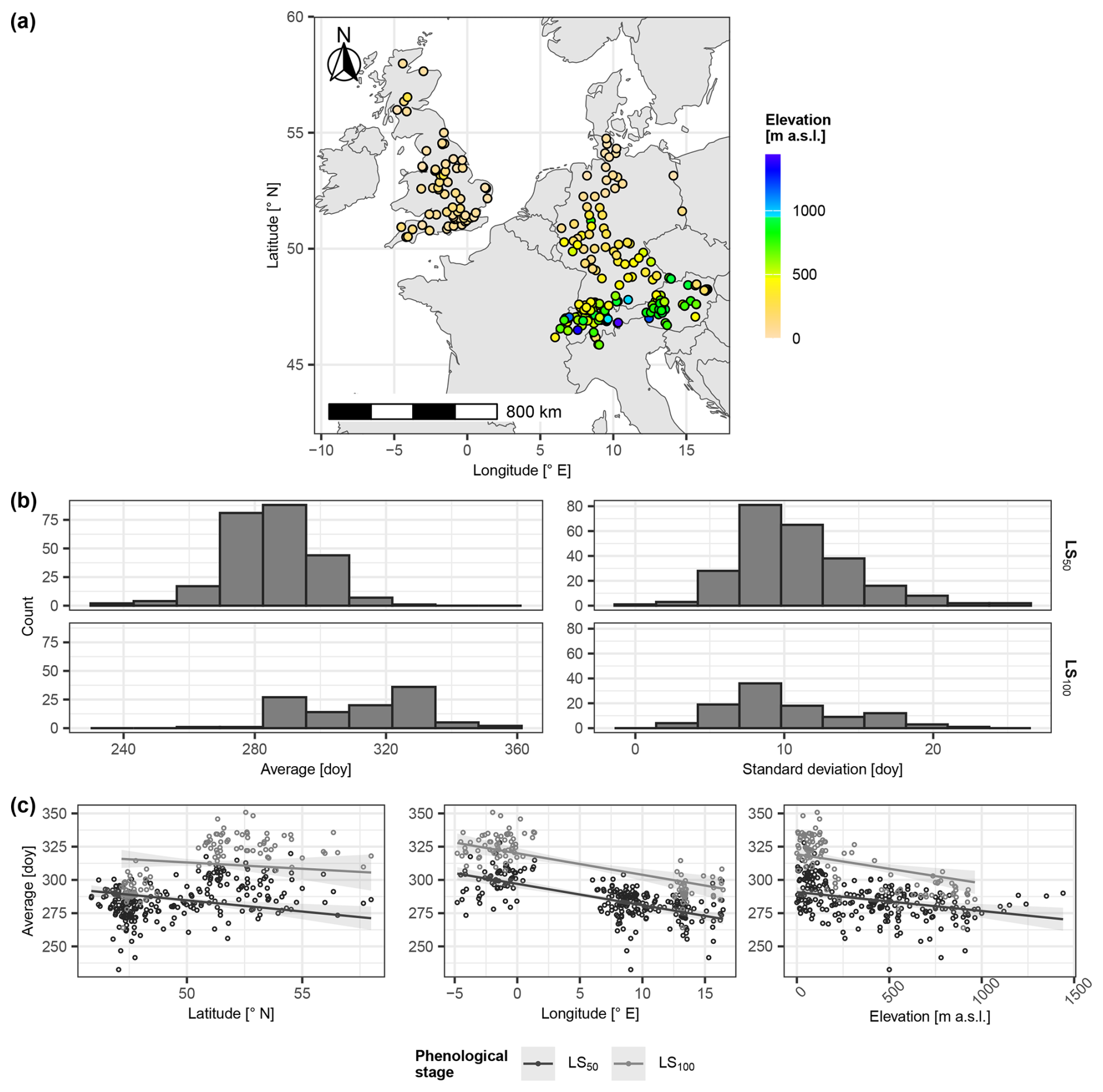
Figure 2 Selected phenological sites. Panel (a) locates the selected sites and indicates corresponding elevation (meters above sea level (m a.s.l.)). In panel (b), the histograms illustrate the distributions of the site-specific average day of year (doy; left) and corresponding standard deviation (right) per leaf senescence stage (i.e., 50 % and 100 % of the leaves having changed color or having fallen (LS₅₀ and LS₁₀₀, respectively); rows). Panel (c) plots the site-specific average doy of LS₅₀ and LS₁₀₀ (grey and black circles, respectively) in relation to site latitude (° N) (left), longitude (° E) (middle), and elevation (m a.s.l.) (right), together with the linear regression lines and corresponding 99 % confidence intervals. The linear regression explained site-specific average LS₅₀ and average LS₁₀₀ by latitude, longitude, and elevation (Sect. S1.1.2). Corresponding estimates were plotted against latitude for mean longitude and mean elevation (left), against longitude for mean latitude and mean elevation (middle), and against elevation for mean latitude and mean longitude.

Table 1 Observations of spring and fall leaf phenology.

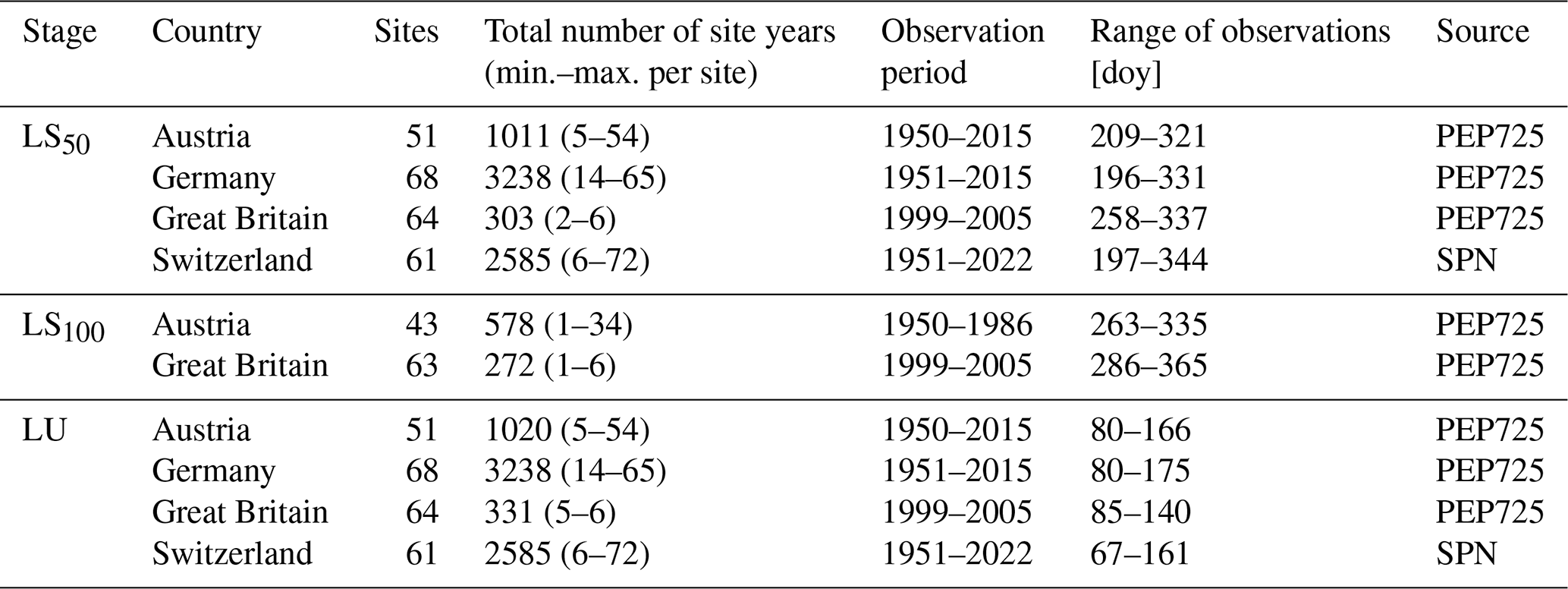
Note: LU refers to the stage when 50 % of the leaves are unfolded. LS₅₀ and LS₁₀₀ refer to the stages with 50 % and 100 % of the leaves, respectively, having changed color or having fallen. The timing of these stages is given by the day of year (doy). A site year is a year for which an observation of both LU and LS₅₀ or LS₁₀₀ was recorded at a given site. Two data sources were considered: PEP725 (Templ et al., 2018) and the Swiss phenological network (SPN; Swiss phenology network, 2025).

We checked all site years with regards to the order and completeness of the phenological observations. Observations of LS₅₀ and LS₁₀₀ that occurred between the day of year (doy) 60 and 151 were discarded, as were observations of LU that occurred after doy 180 or after LS₅₀ or LS₁₀₀. Thus, we considered only site years with an observation for LU that was followed by either LS₅₀ or LS₁₀₀, or by both LS₅₀ and later LS₁₀₀, leaving 5018 sites.

From these sites, we made a pre-selection so that the phenological and geographical range of the LS₅₀ observations was evenly covered and all LS₁₀₀ observations were included. This involved splitting all 5018 sites into 8–10 bins with equal spans for the average and standard deviation of LS₅₀ as well as for latitude, longitude, and elevation, so that each bin contained at least two sites (e.g., the range between doy 232 and 328 for the average LS₅₀ was split into 10 bins of 9.7 d). From each bin, we chose the site with the most LS₅₀ observations, with random choice if this applied to more than one site. These sites were completed by all sites with an LS₁₀₀ observation, resulting in a pre-selection of 7137 LS₅₀ and 850 LS₁₀₀ observations recorded at 244 and 106 sites, respectively.

2.2 Driver data

For each phenological site, weather variables, elevation, and the leaf area index (LAI) were approximated by the weighted averages from octagons with a radius of 2.5 km around the phenological sites, and combined with the atmospheric CO₂ concentration. Daily weather variables and elevation were derived for each site from the E-OBS dataset (Copernicus Climate Change Service, Climate Data Store, 2020; Cornes et al., 2018), which contains interpolated data from a 100-member ensemble driven with meteorological observations. We extracted and approximated site elevation, maximum temperature, mean temperature, minimum temperature, precipitation, relative humidity, and surface shortwave downwelling radiation for 1950–2022. These temperature variables were corrected through day- and site-specific lapse rates to account for elevational differences between the octagon averages and sites (i.e., the elevation according to the phenology datasets or, if missing, according to EU-DEM, 2024, with a resolution of 25 m, and the location according to the phenology datasets). These lapse rates were linearly regressed from the grid cell of a particular site and the eight neighboring grid cells, assuming an elevation of 0 m a.s.l. (meters above sea level) for grid cells over the sea. Occasional gaps in the regressed lapse rates were interpolated with site-specific cubic splines. LAI per site was taken from the remotely sensed monthly LAI (1981–2015) in the GIMMS-LAI3g dataset (version 2; Mao and Yan, 2019). LAI is averaged among years in this dataset, and thus we also used these monthly LAI values for the years 1950–1980. Atmospheric CO₂ concentrations were taken from a reconstructed dataset for the years 1950–2013 and a remotely sensed dataset for the years 2002–2022 (Cheng et al., 2022; Copernicus Climate Change Service, Climate Data Store, 2018). Both datasets provide monthly data, which we distilled into annual averages. These averages were combined through weighted means over the years 2002–2013 to assure a smooth transition between the datasets. As some monthly CO₂ observations between 2002 and 2022 were missing, we used modeled CO₂ values derived from site-specific cubic splines based on the remotely sensed data (Copernicus Climate Change Service, Climate Data Store, 2018).

We further calculated for each site day length, daily photosynthetic activity, and the daily Keetch and Byram drought index (KBDI). Day length was calculated following Brock (1981), using the latitude of each site (Sect. S1.2.1). Daily sink limited photosynthetic activity was calculated following Farquhar et al. (1980) and Collatz et al. (1991), using daily surface shortwave downwelling radiation, day length, and mean temperature together with monthly LAI averaged among years and annual atmospheric CO₂ concentration (Sect. S1.2.2). The daily KBDI was calculated following Keetch and Byram (1968), using precipitation and maximum temperature (Sect. S1.2.3).

2.3 Model conceptualization

Based on the process of leaf development according to Jibran et al. (2013), we defined our model as a one-way process that may be formulated with either two or three phases of leaf development, i.e., either the phases mature and old leaf or the phases young, mature, and old leaf (Figs. 1 and 3). After leaf unfolding, the young leaf is insensitive to stress and ages until it becomes a mature leaf (Fu et al., 2014; Jibran et al., 2013; Keenan and Richardson, 2015). The mature leaf can be affected by stress and ages until it becomes an old leaf (Jan et al., 2019; Jibran et al., 2013; Lim et al., 2007). Senescence induction may be caused by stress in the mature leaf or by aging, in the case of which it coincides with the transition from mature to old leaf, causing the leaf to change color and to fall off (Jan et al., 2019; Jibran et al., 2013; Lim et al., 2007).

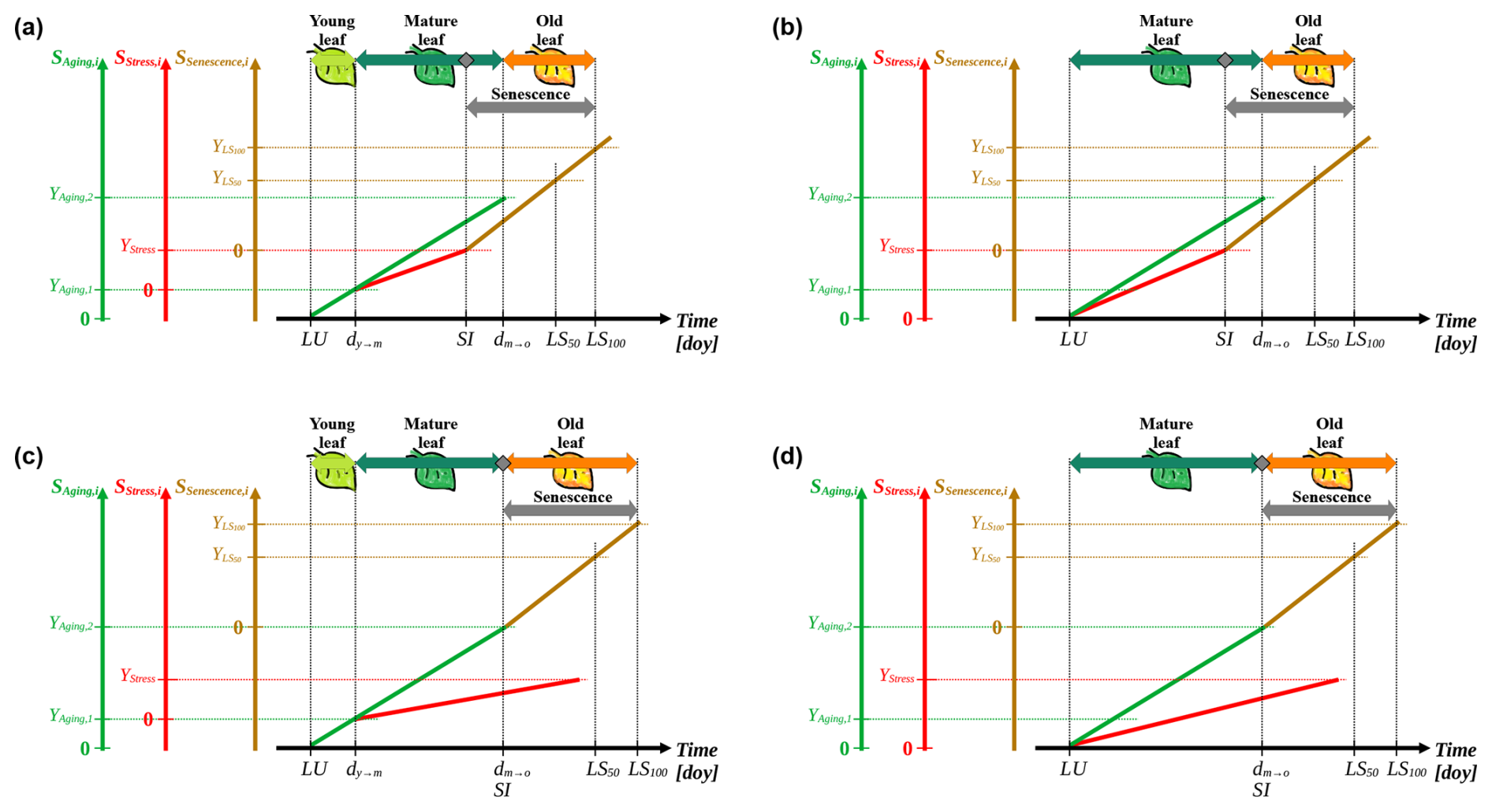
Figure 3 Conceptualization of the leaf development model. The process of leaf development is defined by three subsequent phases of leaf development, i.e., “young leaf”, “mature leaf”, and “old leaf” (light green, dark green, and orange horizontal arrows, respectively; a and c). Alternatively, the process is simplified into two subsequent development phases, i.e., “mature leaf”, and “old leaf” (b, d). Senescence may be induced by stress during the phase of the mature leaf (grey rhombuses; a, b) or by aging on the day of transition from the mature to the old leaf (d_m→o; c, d, respectively). The state of aging, stress, and senescence (y axes; S_Aging,i, S_Stress,i, and S_Senescence,i; Eq. 1; solid green, red, and brown lines, respectively) for day i are derived from the corresponding daily rates (Eqs. 3, 4, and 8) accumulated over time (x axis; day of year (doy)). Starting from the leaf unfolding date (LU), these states simulate the leaf development, marked by transitions from the young to the mature leaf (d_y→m) and d_m→o as well as by the dates of senescence induction (SI) and of the phenological stages 50 % and 100 % leaf coloring or fall (LS₅₀ and LS₁₀₀, respectively). These transitions and stages occur when S_Aging,i, S_Stress,i, and S_Senescence,i reach corresponding thresholds (Y_Aging,1, Y_Aging,2, Y_Stress, $Y_{{\mathrm{LS}}_{\mathrm{50}}}$, and $Y_{{\mathrm{LS}}_{\mathrm{100}}}$). SI is defined as the first day on which either Y_Stress or Y_Aging,2 is reached (a, b versus c, d, respectively) and marks the onset of senescence (grey horizontal arrow), during which the daily senescence rate accumulates. If SI results from Y_Aging,2 being reached, it coincides with d_m→o. Dotted lines are auxiliary lines.

Based on these definitions, we formulated the leaf development process under the following assumptions. Aging may be simulated either by photosynthetic activity (Jibran et al., 2013; Paul and Foyer, 2001; Zohner et al., 2023) or, more simply, by a number of days. Stress may be simulated by a combination of sudden or gradual responses to the stressors cold, shortening day length, drought, heat, frost, heavy rain, and nutrient depletion (Bigler and Vitasse, 2021; Jan et al., 2019; Jibran et al., 2013; Kloos et al., 2024; Mariën et al., 2021; Tan et al., 2023; Wang et al., 2022; Xie et al., 2015, 2018; Zohner et al., 2023). Senescence may be simulated in linear, convex, or sigmoidal dependence on combined aging and stress (Tan et al., 2023; Xie et al., 2015).

All formulations are based on daily states of aging, stress, and senescence (Eq. 1), which are compared to corresponding thresholds (Eq. 2):

$$\begin{array}{}\text{(1)}& {\displaystyle }{S}_{k,j}={\sum }_{i=t_{\mathrm{0},k}}^j{R}_{k,i},\text{(2)}& {\displaystyle }{S}_{k,j}⩾Y_k.\end{array}$$

Here, S_k.j is the state on day j of either aging, stress, or senescence (k). This state is formulated as the sum of the corresponding rates on day i(R_k,i), which accumulated between the starting day t_0,k and j, until the threshold Y_k is reached. In other words, the daily aging rate (R_Aging,i) accumulates from LU ($t_{\mathrm{0},\mathrm{Aging}}=\mathrm{LU}$). The transition from young leaf to mature leaf occurs when S_Aging,j reaches Y_Aging,1. Thus, day j becomes t_0,Stress and the accumulation of the daily stress rate (R_Stress,i) starts, while R_Aging,i continues to accumulate. While the transition from mature leaf to old leaf occurs when S_Aging,j reaches Y_Aging,2, senescence is either induced with this transition or already earlier due to S_Stress,j reaching Y_Stress. Upon senescence induction, day j becomes t_0,Senescence and the daily senescence rate (R_Senescence,i) starts to accumulate. Eventually, S_Senescence,j reaches $Y_{{\mathrm{LS}}_{\mathrm{50}}}$ and $Y_{{\mathrm{LS}}_{\mathrm{100}}}$, and respective LS₅₀ and LS₁₀₀ are marked by the corresponding days j.

R_Aging,i was either set equal to the daily net photosynthetic activity or to one (i.e., A_net [mol C d⁻¹] or 1 [d d⁻¹], respectively), depending on the formulation (Eq. 3):

$$\begin{array}{}\text{(3)}& R_{\mathrm{Aging},i}=\left\{\begin{array}{l}{A}_{\mathrm{net},i},\\ \mathrm{1}.\end{array}\right.\end{array}$$

R_Stress,i was formulated as the sum of three to seven weighted stressors (D_stress; Eqs. 4–6), always considering (1) cold days (derived from minimum temperature; T_n [°C]), (2) shortening days (derived from the difference in day length; δL [h], with $\mathit{\delta }{L}_i=L_i-L_{i-\mathrm{1}}$), and (3) dry days (approximated by KBDI; Q). In addition, some formulations of R_Stress also considered (4) periods of heavy rainfall (approximated by the 5 d precipitation; P₅ [mm], with $P_{{\mathrm{5}}_i}$ being the sum of P_i−4 to P_i), (5) heat days (derived from maximum temperature; T_x [°C]), (6) nutrient depletion (approximated by the accumulated A_net since LU, due to the absence of soil data), and/or (7) frost days (through a response to T_n with lower thresholds than for cold days; Table S3 in the Supplement):

$$\begin{array}{}\text{(4)}& {\displaystyle }{R}_{\mathrm{Stress},i}=\sum w_{D_{\mathrm{Stress}}}\times f\left(D_{\mathrm{Stress},i}\right),\text{(5)}& {\displaystyle }{D}_{\mathrm{Stress},i}\in \left\{T_{n_i},\mathit{\delta }{L}_i,Q_i,P_{{\mathrm{5}}_i},T_{x_i},{\sum }_{l=d_{\mathrm{LU}}}^i{A}_{\mathrm{net},l},T_{{\mathrm{n}}_i}\right\},\text{(6)}& {\displaystyle }f\left(x\right)=\left\{\begin{array}{l}g\left(x\right),\\ h\left(x\right).\end{array}\right.\end{array}$$

Here, $w_{D_{\mathrm{Stress}}}$ is the weight for the response [f(x)] to D_Stress, calculated according to g(x) or h(x) (Eqs. 7 and 8):

$$\begin{array}{}\text{(7)}& {\displaystyle }g\left(x\right)=\left\{\begin{array}{ll}\mathrm{1}& \text{if}x\ge a,\\ \mathrm{0}& \text{if}x<a,\end{array}\right.\text{(8)}& {\displaystyle }h\left(x\right)=\left\{\begin{array}{ll}\mathrm{1}& \text{if}x<b_{\mathrm{0}},\\ \frac{b_{\mathrm{1}}-x}{b_{\mathrm{1}}-b_{\mathrm{0}}}& \text{if}{b}_{\mathrm{0}}\le x\le b_{\mathrm{1}},\\ \mathrm{0}& \text{if}x>b_{\mathrm{1}}.\end{array}\right.\end{array}$$

While a marks the sudden boundary between an unstressed and stressed state, b₀ and b₁ mark the lower and upper bounds, respectively, between which stress gradually increases (Fig. 4). Because stress results when x≥a and x≥b₀, the response to δL and T_n was formulated as g(−δL) and g(−T_n) as well as h(−δL) and h(−T_n). This translates into stress if $\mathit{\delta }L\le -a$, $\mathit{\delta }L\le -b_{\mathrm{0}}$, $T_n\le -a$, and $T_n\le -b_{\mathrm{0}}$. For example, if stress occurs suddenly or gradually when $\mathit{\delta }L\le -\mathrm{0.01}$ h, then a=0.01 h and b₀=0.01 h, respectively. Note that these are examples, see Table 3 for the calibrated values.

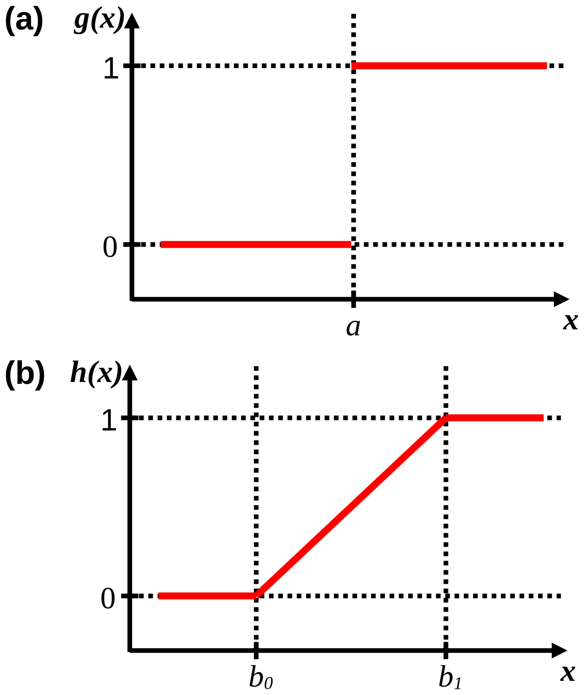
Figure 4 Response functions (solid red lines) of g(x) and h(x). In panel (a), a marks the boundary value of x at which g(x) suddenly changes from 0 to 1 (i.e., from no effect to an effect). In panel (b), b₀ and b₁ mark the lower and upper bounds of x, respectively, between which f(x) gradually increases from 0 to 1. Dotted lines are auxiliary lines.

R_Senescence,i was either formulated as the sum, product, or exponential function of R_Aging,i and R_Stress,i or of S_Aging,i and R_Stress,i, which yield linear, convex, and sigmoid curves, respectively (Eq. 9):

$$\begin{array}{}\text{(9)}& R_{\mathrm{Senescence},i}=\left\{\begin{array}{l}{w}_{\mathrm{A}}{R}_{\mathrm{Aging},i}+w_{\mathrm{S}}{R}_{\mathrm{Stress},i}\\ s_X\left(R_{\mathrm{Aging},i}\times R_{\mathrm{Stress},i}^{x_{\mathrm{S}}}\right)\\ s_X\frac{\mathrm{1}}{e^{c{S}_{\mathrm{Aging},i}\left(d-R_{\mathrm{Stress},i}\right)}}\end{array}.\right.\end{array}$$

w_A and w_S are the weights of R_Aging and R_Stress, respectively, and s_X is a scaling factor, all of which allowed us to hard code $Y_{{\mathrm{LS}}_{\mathrm{50}}}=\mathrm{1}$, x_S is the range bounded exponent of R_Stress, while c and d are the parameters of the sigmoid curve that relates R_Stress and S_Aging (Lang et al., 2019).

2.4 Model calibration and validation

We selected the observations for the calibration and validation samples with different procedures. To have a low risk of overfitting (i.e., the bias–variance trade-off; Sect. 2.2.2 in James et al., 2017), each calibration sample contained at least 10 observations per calibrated parameter (Meier and Bigler, 2023). We defined two calibration datasets: one to calibrate a model that predicts both LS₅₀ and LS₁₀₀ simultaneously, and one to calibrate a model that predicts LS₅₀ only. For the two datasets, we identified the site years with the most extreme conditions during the growing season, i.e., the hottest, coldest, and driest 10 d periods observed between LU and LS₅₀ as well as the shortest and longest growing season observed in the pre-selected data (Sect. 2.1). For the first dataset, hereafter called “LS₅₀–LS₁₀₀ sample”, we randomly selected 250 of these site years containing an observation for both LS₅₀ and LS₁₀₀. For the second dataset, hereafter referred to as “LS₅₀ sample”, we randomly selected 250 of these site years containing observations for LS₅₀. These calibration samples were paired with validation samples that contained all remaining LS₅₀ and LS₁₀₀ observations or all remaining LS₅₀ observations, respectively. We drew both the LS₅₀ and LS₅₀–LS₁₀₀ samples twice. While model development was based on the LS₅₀–LS₁₀₀ samples, model evaluation was based on the LS₅₀ sample to allow for a comparison with previously published models. All models were calibrated five times per drawn sample (i.e., 10 “calibration runs” per model and LS₅₀ sample or LS₅₀–LS₁₀₀ sample) by minimizing the root mean squared error (RMSE; Eq. S44) with generalized simulated annealing and optimal, model-specific controls (see Sect. S2.2; Xiang et al., 1997, 2017).

2.5 Model development

We based our model on the most accurate formulation of the leaf development process after testing different formulations in several iterations (Fig. 5; see Table S3 for parameter ranges). First, we defined the process structure based on sudden responses (g(x); Eq. 7) to the stressors for cold days, shortening days, and dry days. In iteration 1, we tested the definition of the aging rate (R_Aging) and of the senescence rate (R_Senescence) based on the two phases of leaf development “mature leaf” and “old leaf” (Fig. 3b and c). R_Aging was formulated as a function of either the net photosynthetic activity (A_net) or of the number of days (Eq. 3). R_Senescence was formulated in linear, convex, or sigmoidal dependence on combined aging and stress (through R_Aging or the state of aging (S_Aging) and through the stress rate (R_Stress)) in either a sum, product, or exponential function (Eq. 9). In iteration 2, we tested the number of phases of leaf development and added the phase “young leaf” (Fig. 3a and d). Thus, we formulated R_Stress with gradual responses (h(x); Eq. 8) to the initial stressors and a forward selection of additional stressors. In iteration 3, we considered each stressor for cold days, shortening days, and dry days through h(x) rather than g(x). In iteration 4, we considered one additional stressor, i.e., heavy rain periods, heat days, nutrient depletion, or frost days through g(x). In iteration 5, we considered the additional stressor through h(x) rather than g(x). In iteration 6, the procedure of iterations 4 and 5 was repeated as long as they resulted in a formulation that was selected for further development.

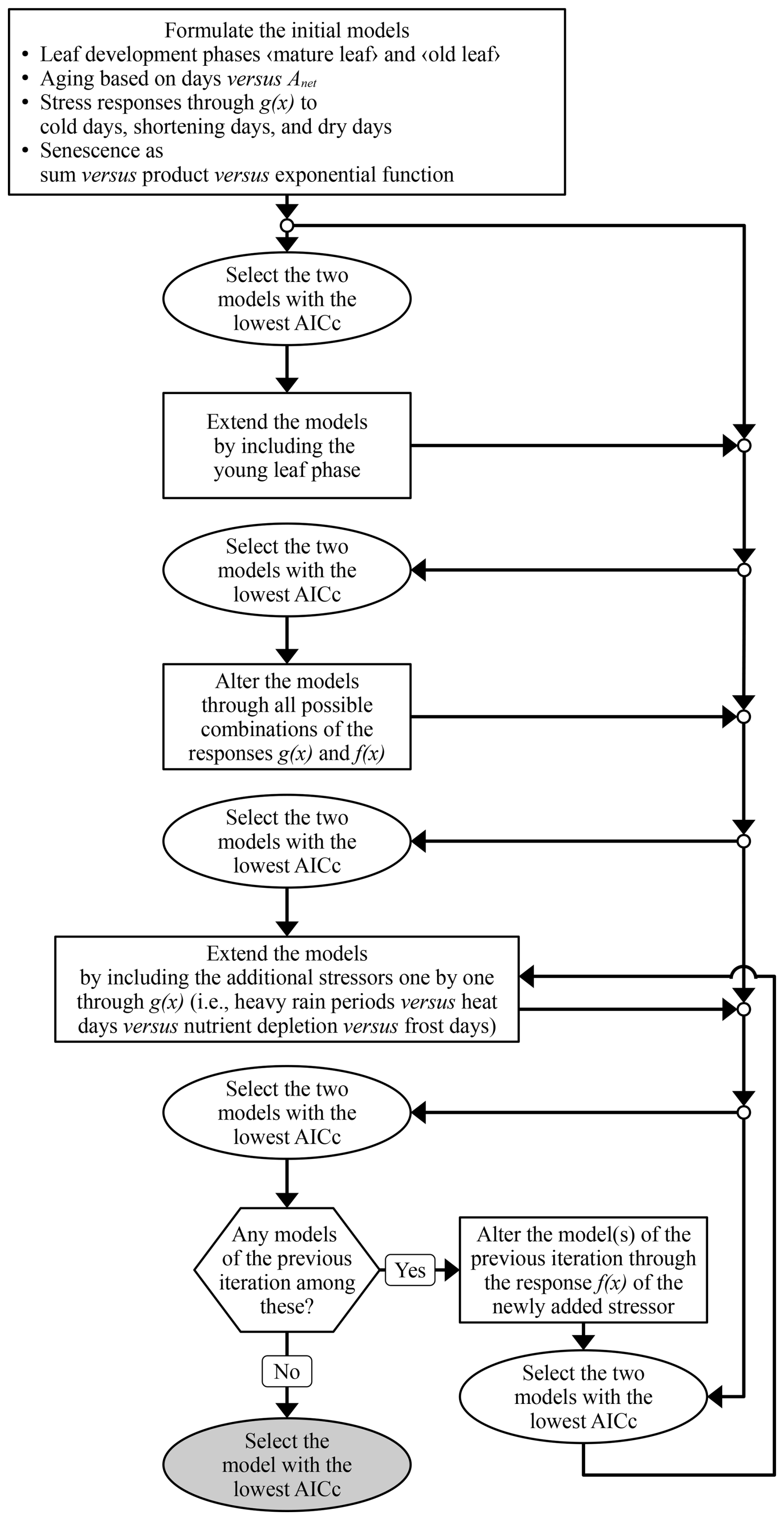
Figure 5 Model development. The iterations of model development are symbolized with rectangles. Selection of the best formulated models (ellipses) was based on the Akaike information criterion corrected for small samples (AICc; Eq. S41; Akaike, 1974; Burnham and Anderson, 2004) and the final selection is marked in grey. For the response functions g(x) and h(x), see Eqs. (7) and (8).

The formulations to be further developed were selected according to the accuracy of the corresponding model in predicting LS₅₀ and LS₁₀₀, i.e., through calibration with the LS₅₀–LS₁₀₀ sample. This accuracy was assessed with the Akaike information criterion corrected for small samples (AICc; Eq. S41 in the Supplement; Akaike, 1974; Burnham and Anderson, 2004), which accounts for both the goodness of fit between the predicted and observed leaf senescence dates and the number of free parameters. The AICc was calculated for each calibration run (see Sect. 2.4) and the run with the highest AICc per model was excluded. We further developed the formulations of the two models with the lowest median AICc across the given and all previous iterations. Finally, the model with the lowest median AICc was selected and further evaluated.

2.6 Model evaluation

First, we evaluated the functionality of the selected model. We were particularly interested in the causes of senescence induction that could be due to aging or stress (Fig. 3). We counted how often aging versus stress induced senescence, and we quantified the relative amount of accumulated stress caused by each stressor at the time of senescence induction. We compared both aging- and stress-induced senescence as well as the relative amounts of stress across mean annual temperature (MAT; °C), mean annual KBDI (MAQ), latitude (LAT; ° N), and elevation (ELV; m a.s.l.) for the given year and site. While MAT and MAQ were assumed to directly affect cold and dry stress, LAT relates to day length through the inclination angle of Earth (Brock, 1981), and ELV relates to dry stress through decreasing nutrients with elevation (Huber et al., 2007; Loomis et al., 2006). The evaluation was based on the calibration runs that resulted in the highest modified Kling–Gupta efficiency (KGE^′; Eq. S45; Gupta et al., 2009; Kling et al., 2012), which combines bias, variability, and correlation of the predicted and observed leaf senescence dates.

Second, we compared the accuracy of the selected model to three previously published models, i.e., the CDD, DM2, and PIA models. Because these models simulate only one stage of leaf senescence, which usually is LS₅₀, we based our comparison on this stage (Delpierre et al., 2009; Dufrêne et al., 2005; Zani et al., 2020). The CDD model determines LS₅₀ by the time the cold degree days reaches a particular threshold (Dufrêne et al., 2005). The DM2 model accumulates the product of temperature differences and day length ratios to corresponding thresholds until the threshold that determines LS₅₀ is reached (Delpierre et al., 2009). The PIA model accumulates temperatures and day lengths that are combined in an exponential function, and derives the threshold to determine LS₅₀ from the photosynthetic activity during the growing season (Zani et al., 2020). All these models were compared based on the calibration run that resulted in the highest KGE^′. Further, we compared the RMSE and AICc as well as the Pearson correlation (ρ) across the entire validation sample (ρ_Overall), across space (ρ_Spatial), and across time (ρ_Temporal). ρ_Spatial was calculated across sites based on their mean predicted and observed LS₅₀. ρ_Temporal was calculated for each site, based on the yearly predicted and observed LS₅₀.

Third, we estimated the extent to which the model error (i.e., predicted minus observed LS₅₀) was affected by data structure as well as by climatic and spatial deviations from the LS₅₀ calibration sample, using a linear mixed-effects model (LMM; Pinheiro and Bates, 2000) and an analysis of variance (ANOVA; Sect. S2.4; Fox, 2016). In the LMM, the response variable “model error” was explained by the factor variable “country” as well as the interaction of the factor variable “model” with each of the differences between a site year and the average of the calibration sample in MAT (δMAT), MAQ (δMAQ), the accumulated A_net between LU and summer solstice (δA_net), latitude (δLAT), and elevation (δELV). The random intercept was grouped by “site”. The LMM was fitted with fast restricted maximum likelihood (Wood, 2011), and served as basis for the ANOVA. This type-III ANOVA (Yates, 1934) quantified the impact of the explanatory variables on the variance of the model error that was explained by the LMM. The impact attributable to data structure was caused by the fixed effects of “country” and the standard deviation in the random intercepts grouped by “site”, while the impacts attributable to climatic versus spatial deviations from the calibration sample was caused by the effects of δMAT, δMAQ, and δA_net versus the effects of δLAT and δELV, respectively.

2.7 Statistical software and reporting of results

We used the programming language R, together with the R package data.table for data processing (Barrett et al., 2024). In R, data from xslx files were extracted with the R package readr (Wickham et al., 2024), and data from netCDF files were extracted and averaged with the R packages ncdf4 (Pierce, 2023), raster (Hijmans, 2023), sf (Pebesma, 2018; Pebesma and Bivand, 2023), and sp (Bivand et al., 2013; Pebesma and Bivand, 2005). Leap years were identified with the function leap_year in the R package lubridate (Grolemund and Wickham, 2011). Gaps in the regressed lapse rates were filled with the function na.spline in zoo (Zeileis and Grothendieck, 2005). Seasonal splines of atmospheric CO₂ concentrations were calculated with the function sm in npreg (Helwig, 2024). The leaf senescence models were calibrated with the R package GenSA (Xiang et al., 2013), while the LMM was fitted with the R package mgcv (Wood, 2017) and the ANOVA was calculated with the R package stats (R Core Team, 2025). LMM estimates and 99 % confidence intervals (i.e., significance level α=0.01) for combined coefficients, e.g., the effect of δMAT for a given model, were calculated with the Delta method (chap. 5.1.4 in Fox and Weisberg, 2019; chap. 9.9 in Wasserman, 2004) through the function deltaMethod in the R package car (Fox and Weisberg, 2019). For each LMM coefficient and ANOVA impact, we expressed the most optimistic change of odds between the null hypothesis (being zero; H₀) and alternative hypothesis (being different from zero or greater than zero, respectively; H₁) with the minimum Bayes factor (BF₀₁), labeling H₀ : H₁ ratios of 1/1000 and 1/100 as “decisive” and “very strong”, respectively (Held and Ott, 2018; Johnson, 2005). BF₀₁ was calculated from the p values and number of data with the function tCalibrate in the R package pCalibrate (Held and Ott, 2018). For the visualizations, we used the R packages ggplot and ggpubr (Kassambara, 2020; Wickham, 2016), as well as the R packages ggspatial and rnaturalearth for the maps (Dunnington, 2023; Massicotte and South, 2023).

3 Results

3.1 Model formulation – the DP3 model

We tested 34 formulations of the leaf development process through 1428 calibration runs, and found that three subsequent leaf development phases resulted in the most accurate model (according to the AICc; Figs. 3a, c, 6, and S1–S2 in the Supplement). In this model, the phase “young leaf” starts with leaf unfolding. As a daily aging rate R_Aging accumulates (Eq. 10), the simulated state of aging increases by 1 day per day. When this state reaches the threshold Y_Aging,1 (Eqs. 1 and 2), the phase “mature leaf” begins. During this phase, the leaf continues to age and is also sensitive to stress caused by cold days, shortening days, and dry days, to which we hereafter refer to as “cold stress”, “photoperiod stress”, and “dry stress”, respectively. This stress is summarized in a daily stress rate (R_Stress; Eq. 11) and thus accumulated to determine the state of stress. The first day that either the state of stress or the state of aging reaches the respective thresholds Y_Stress or Y_Aging,2 (Eqs. 1 and 2), senescence is induced, while the phase “old leaf” starts only when the state of aging reaches Y_Aging,2. Once senescence is induced, a daily senescence rate (R_Senescence) in convex dependence on stress accumulates (Eq. 12) and determines the state of senescence. The days this state reaches the thresholds $Y_{{\mathrm{LS}}_{\mathrm{50}}}$ and $Y_{{\mathrm{LS}}_{\mathrm{100}}}$ (Eqs. 1 and 2) correspond to the predicted dates of LS₅₀ and LS₁₀₀, respectively. Hereafter, we refer to this model as “DP3” model (Tables 2 and 3; Meier, 2025b, coded in R).

$$\begin{array}{}\text{(10)}& {\displaystyle }{R}_{\mathrm{Aging},i}=\mathrm{1}\text{(11)}& {\displaystyle }{R}_{\mathrm{Stress},i}=w_{C}g\left(-T_{n_i}\right)+w_{P}g\left(-\mathit{\delta }{L}_i\right)+w_{D}g\left(Q_i\right)\text{(12)}& {\displaystyle }{R}_{\mathrm{Senescence},i}=s_X{R}_{\mathrm{Stress},i}^{x_{\mathrm{S}}}\end{array}$$

Here, w_C, w_P, and w_D are the weights for the response functions g(x) (Eq. 7) to the minimum temperature (T_n), difference in day length (δL), and KBDI (Q) on day i, respectively (e.g., w_Pg(−δL_i) results in the photoperiod stress on day i). s_X is the scaling factor for R_Stress, which is shaped by x_S.

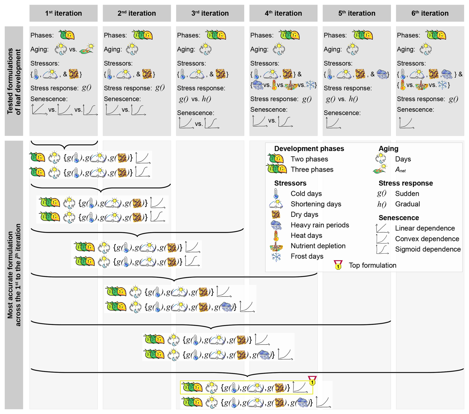
Figure 6 Tested model formulations. The tested formulations differed in their number of leaf development phases (i.e., two or three phases), in their driver of the aging rate (i.e., days or photosynthetic activity (A_net)), their stress rate in response (i.e., g(x) or h(x)) to the stressors cold, shortening, dry, heat, and frost days, heavy rain periods, and nutrient depletion, and their dependence of the senescence rate on aging and stress (i.e., linear, convex, or sigmoid dependence as a the result of a sum, product, or exponential function, respectively). After each iteration, we identified the two most accurate formulations across the given and all previous iterations (Fig. 5, Sect. 2.5). These formulation were further developed through the next iteration. As soon as an iteration did not produce any new model formulations, we selected the more accurately formulated model (“top formulation”; i.e., the “DP3” model). All formulations were tested for beech based on the LS₅₀–LS₁₀₀ sample (Sect. 2.4).

Table 2 Input and output variables of the DP3 model.

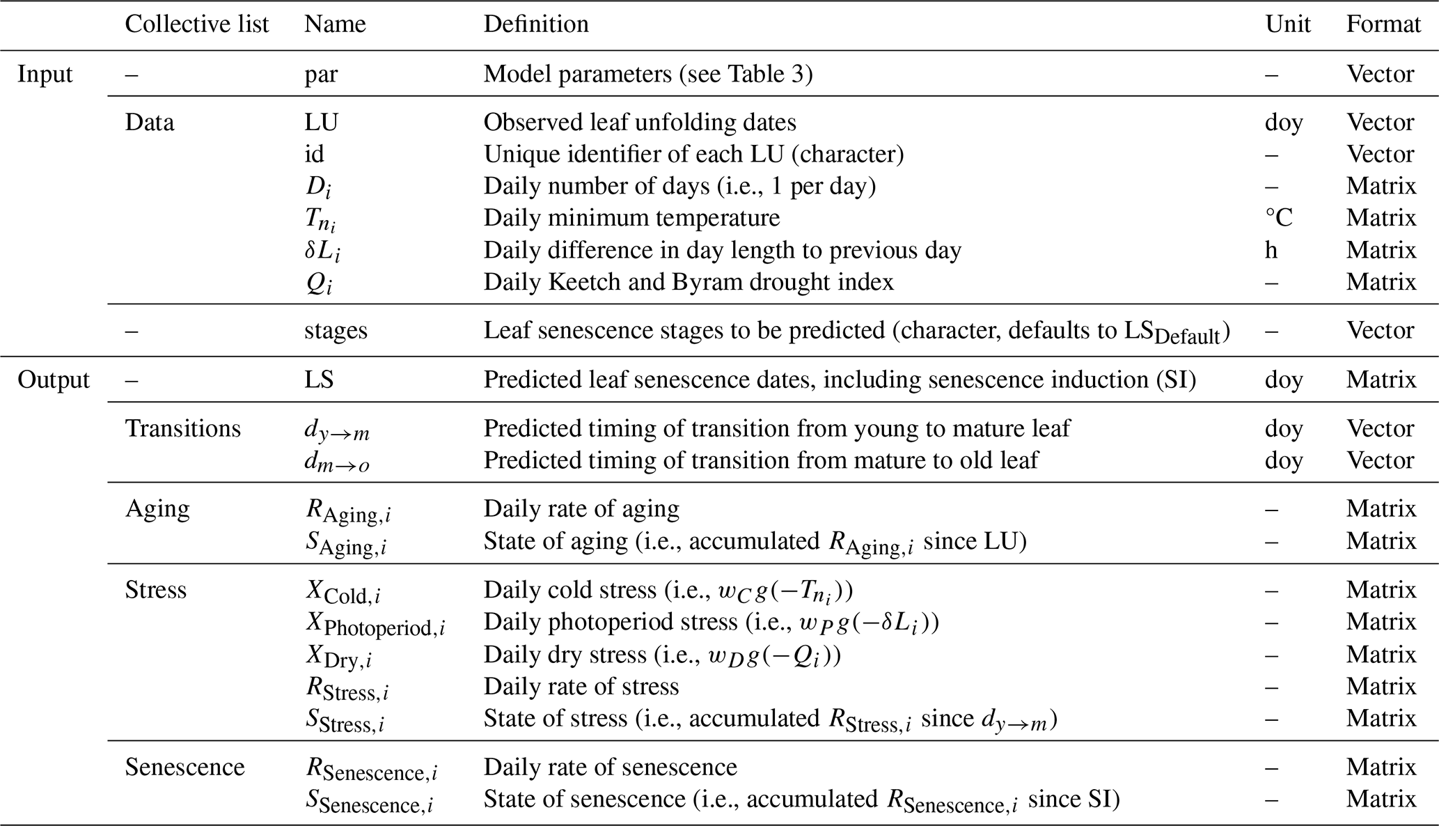
Note: daily variables refer to day i, and accumulated variables refer to the period until day i. The vector par contains the model parameters listed in Table 3. In the collective lists data, aging, stress, and senescence, the rows of the matrices refer to the days of the year, while the columns refer to site years and are ordered identically between all matrices. This order matches the order of the vectors in the collective lists data and transition. For the LS matrix, the rows refer to the site years and the columns refer to the senescence induction date and the dates of the leaf senescence stages indicated by the vector stages. LU, LS, d_y→m, and d_m→o are given in day of year (doy; Meier, 2025b).

Table 3 Fitted parameters of the DP3 model.

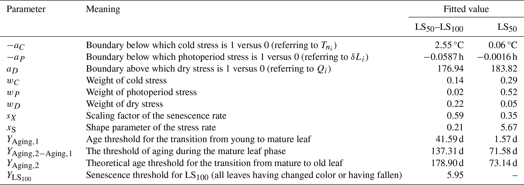
Note: the parameters refer to Eqs. (7) and (9)–(11) and were fitted for beech with the LS₅₀ and LS₅₀–LS₁₀₀ samples (Sect. 2.4). All of the parameters were calibrated within the initial ranges (Table S3) to their fitted value. To avoid fitted values of $Y_{\mathrm{Aging},\mathrm{1}}>Y_{\mathrm{Aging},\mathrm{2}}$, we used and calibrated $Y_{\mathrm{Aging},\mathrm{2}-\mathrm{Aging},\mathrm{1}}$ instead of Y_Aging,2. The theoretical threshold Y_Aging,2 was not calibrated but calculated from $Y_{\mathrm{Aging},\mathrm{1}}+Y_{\mathrm{Aging},\mathrm{2}-\mathrm{Aging},\mathrm{1}}$ and displayed for easier interpretation. The thresholds for stress (Y_Stress) and LS₅₀ ($Y_{{\mathrm{LS}}_{\mathrm{50}}}$; i.e., the time of 50 % of the leaves having changed color or having fallen) were hard coded with Y_Stress=1 and $Y_{{\mathrm{LS}}_{\mathrm{50}}}=\mathrm{1}$. The shortening of a day length of 0.0016 h (a_P, corresponding to 0.1 min) based on the LS₅₀ calibration is reached on doys 175, 174, and 174 (i.e., 24, 23, and 23 June) at the exemplary minimum, median, and maximum latitudes of our samples (i.e., 45.9° N, 47.8° N, and 58.0° N), respectively. Alternatively, the shortening of 0.0587 h (3.5 min) based on the LS₅₀–LS₁₀₀ calibration is reached on doys 252 and 202 (i.e., 9 September and 21 July) at the median and maximum latitudes of our samples, respectively, whereas it is never reached at the minimum latitude.

According to the DP3 model, leaf senescence was generally induced earlier during warmer years and at lower elevations (Fig. 7; Tables S5–S8). In average, senescence was induced a month earlier when mean annual temperatures were 13–15 °C than when they were 4–6 °C (i.e., 29 May versus 22 June and 20 April versus 12 May when the DP3 model was calibrated with the LS₅₀–LS₁₀₀ and LS₅₀ samples, respectively; hereafter referred to as “DP3${}_{{\mathrm{LS}}_{\mathrm{50}}{\text{–LS}}_{\mathrm{100}}}$ model” and “DP3${}_{{\mathrm{LS}}_{\mathrm{50}}}$ model”; Sect. 2.4). Accordingly, senescence induction was 20 d earlier below 288 m a.s.l. than above 1150 m a.s.l. (i.e., 5 June versus 25 June and 26 April versus 16 May based on the DP3${}_{{\mathrm{LS}}_{\mathrm{50}}{\text{–LS}}_{\mathrm{100}}}$ and DP3${}_{{\mathrm{LS}}_{\mathrm{50}}}$ model, respectively). Both the DP3${}_{{\mathrm{LS}}_{\mathrm{50}}{\text{–LS}}_{\mathrm{100}}}$ model and DP3${}_{{\mathrm{LS}}_{\mathrm{50}}}$ model predicted generally longer-lasting senescence (i.e., the duration between senescence induction and LS₅₀ or LS₁₀₀) during years of higher mean annual temperatures (Fig. S3; Tables S5–S8).

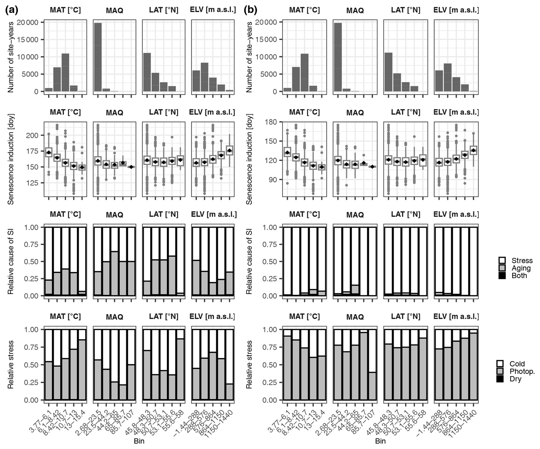
Figure 7 Senescence induction. Panels (a) and (b) are based on simulations by the DP3 model calibrated with the LS₅₀–LS₁₀₀ versus LS₅₀ samples, respectively (Sect. 2.4). The top row of each panel shows the number of site years in the bins, which were equally distributed among mean annual temperature (MAT; °C), mean annual Keetch and Byram drought index (MAQ), latitude (LAT; ° N), and elevation (ELV; m a.s.l.). The second row of each panel visualizes the senescence induction (SI) dates in day of year (doy). While the mean and median dates are marked with black dots and grey lines, respectively, the most extreme values are indicated with dots if outside ±1.5 times the inner quartile range from the 1st and 3rd quartiles and with whiskers otherwise. The third row of each panel illustrates the relative number of site years during which senescence was induced by stress versus aging or by both stress and aging (i.e., both the accumulated stress and aging rates reached their thresholds for SI on the same date). The bottom row of each panel shows the relative amounts of cold stress, photoperiod stress (Photop.), and dry stress that accumulated at stress-caused SI.

Stress induced senescence 2 times and 40 times more often than aging according to the DP3${}_{{\mathrm{LS}}_{\mathrm{50}}{\text{–LS}}_{\mathrm{100}}}$ and DP3${}_{{\mathrm{LS}}_{\mathrm{50}}}$ model, respectively (Fig. 7, Tables S5–S8). Thus, while aging was of negligible importance to senescence induction according to the DP3${}_{{\mathrm{LS}}_{\mathrm{50}}}$ model, it mattered according to the DP3${}_{{\mathrm{LS}}_{\mathrm{50}}{\text{–LS}}_{\mathrm{100}}}$ model, particularly during years of medium mean annual temperature (6–13 °C) as well as at sites of medium latitude (48.3–55.6° N) and of low elevation (below 576 m a.s.l.). At the time of senescence induction due to stress, the amounts of accumulated photoperiod stress and cold stress relative to total stress were 56 % versus 44 % (DP3${}_{{\mathrm{LS}}_{\mathrm{50}}{\text{–LS}}_{\mathrm{100}}}$ model) and 77 % versus 23 % (DP3${}_{{\mathrm{LS}}_{\mathrm{50}}}$ model), respectively, while the corresponding amounts of dry stress were 0.5 % and 0.0 %. Photoperiod stress dominated mostly in warm years and medium-elevation sites according to the DP3${}_{{\mathrm{LS}}_{\mathrm{50}}{\text{–LS}}_{\mathrm{100}}}$ model, whereas it did so in cool years and high-elevation sites according to the DP3${}_{{\mathrm{LS}}_{\mathrm{50}}}$ model. In summary, photoperiod stress rather than cold and dry stress induced leaf senescence, but the importance of these stressors and their dependency on climatic conditions and location differed between the DP3${}_{{\mathrm{LS}}_{\mathrm{50}}{\text{–LS}}_{\mathrm{100}}}$ and DP3${}_{{\mathrm{LS}}_{\mathrm{50}}}$ models.

Accordingly, the relative importance of these stressors for the duration of senescence differed between the DP3${}_{{\mathrm{LS}}_{\mathrm{50}}{\text{–LS}}_{\mathrm{100}}}$ and DP3${}_{{\mathrm{LS}}_{\mathrm{50}}}$ model (Fig. S3; Tables S5–S8). Photoperiod stress clearly dominated the progress from senescence induction to LS₅₀ according to the DP3${}_{{\mathrm{LS}}_{\mathrm{50}}}$ model. However, according to the DP3${}_{{\mathrm{LS}}_{\mathrm{50}}{\text{–LS}}_{\mathrm{100}}}$ model and especially during cool years, cold stress was most important between senescence induction and LS₅₀, whereas photoperiod stress was most important between senescence induction and LS₁₀₀.

3.2 Model accuracy

Leaf senescence dates were predicted with similar accuracy by the DP3 model as by previous models (Fig. 8; Table 4). All models calibrated with the LS₅₀ sample resulted in an RMSE of ∼ 15 d, with the lowest RMSE for the Null model (i.e., constant prediction of each the average LS₅₀ and LS₁₀₀ observations in the calibration sample). The LS₅₀–LS₁₀₀ sample yielded considerably higher RMSE for both the DP3${}_{{\mathrm{LS}}_{\mathrm{50}}{\text{–LS}}_{\mathrm{100}}}$ and Null model, i.e., 23–25 and 18–21 d, respectively. Nevertheless, the DP3${}_{{\mathrm{LS}}_{\mathrm{50}}{\text{–LS}}_{\mathrm{100}}}$ model resulted in the highest overall correlation (ρ_Overall of 0.2 for LS₁₀₀). The highest correlation across space was obtained with the PIA model (ρ_Spatial of 0.4), while the DP3 model resulted in the highest correlation across time (average ρ_Temproal of 0.05 according to DP3${}_{{\mathrm{LS}}_{\mathrm{50}}}$ and according to DP3${}_{{\mathrm{LS}}_{\mathrm{50}}{\text{–LS}}_{\mathrm{100}}}$ for LS₁₀₀).

Table 4 Model accuracy.

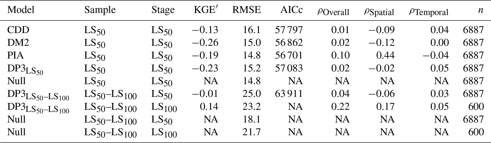
Note: the Null model constantly predicts the average observation in the calibration sample (i.e., the stages with either 50 % or 100 % of the leaves having changed color or having fallen: LS₅₀ or LS₁₀₀, respectively). The modified Kling–Gupta efficiency (KGE^′), root mean squared error (RMSE), Akaike information criterion for small samples (AICc), and Pearson correlation overall, across space, and across time (ρ_Overall, ρ_Spatial, and average ρ_Temporal (ρ_Temporal), respectively) are explained in Sects. 2.6, S2.1, and S2.2. All of these metrics were calculated for the predicted and observed dates in the validation samples LS₅₀ and LS₅₀–LS₁₀₀ (Sect. 2.4). Except for the RMSE, they result in NA if the variance of the predicted dates is zero, which is the case for the Null model. In addition, the AICc for the stage LS₁₀₀ according to the model DP3${}_{{\mathrm{LS}}_{\mathrm{50}}{\text{–LS}}_{\mathrm{100}}}$ was omitted because n, i.e., the number of observations in the validation sample, differed between LS₁₀₀ and LS₅₀. NA – not available.

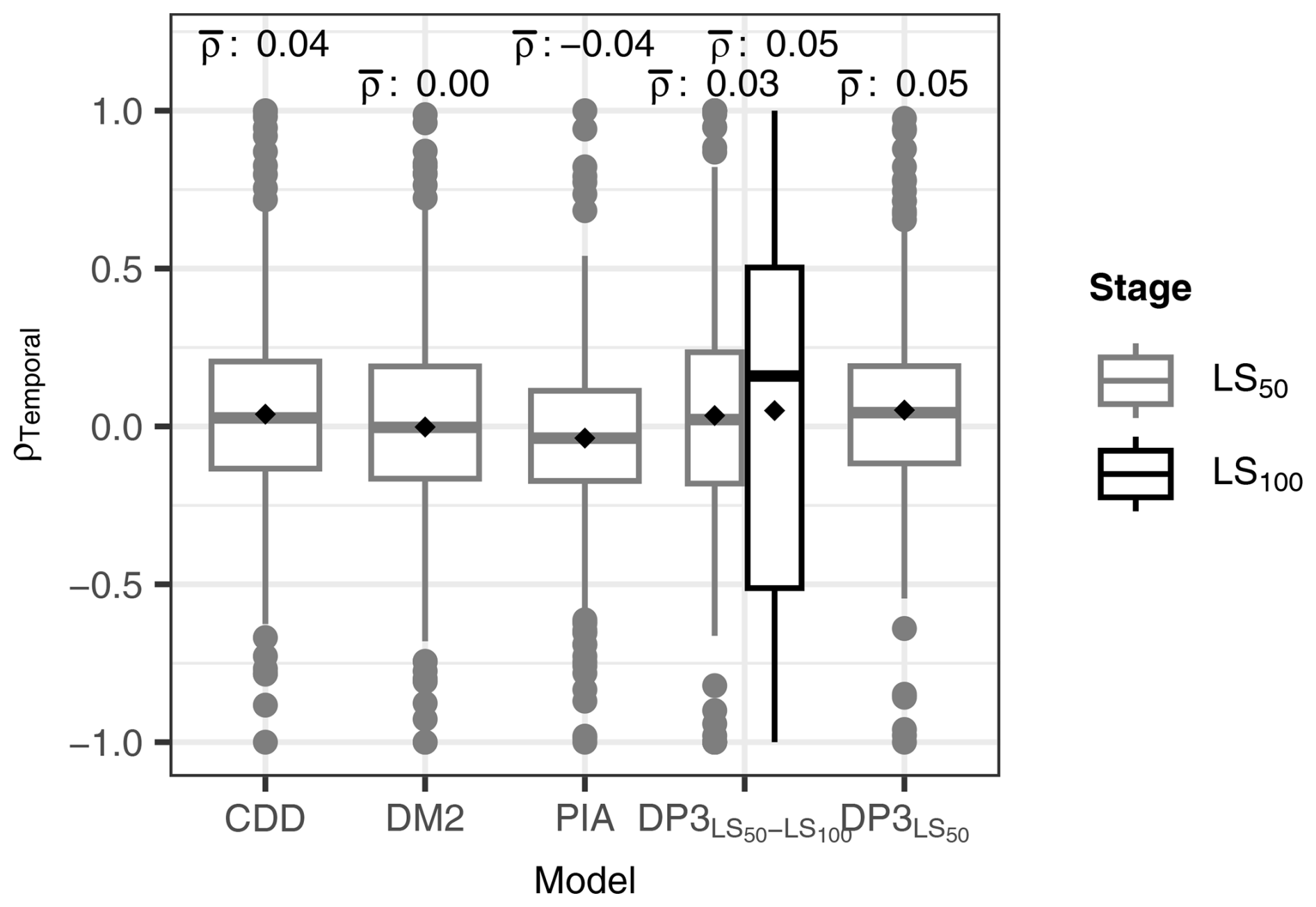
Figure 8 Temporal Pearson correlation (ρ_Temporal). The distribution of ρ_Temporal per site between predicted and observed leaf senescence (the dates when 50 % and 100 % of the leaves having changed color or having fallen (LS₅₀ and LS₁₀₀, respectively)) is displayed for each model. The DP3 model was calibrated twice, i.e., with the LS₅₀–LS₁₀₀ sample (DP3${}_{{\mathrm{LS}}_{\mathrm{50}}{\text{–LS}}_{\mathrm{100}}}$) and with the LS₅₀ sample (DP3${}_{{\mathrm{LS}}_{\mathrm{50}}}$; Sect. 2.4), the latter of which was also used to calibrate the CDD, DM2, and PIA models. The mean ρ_Temporal (black rhombuses) is indicated above each box (ρ). The boxes indicate the inner quartile range and the median (middle line). The most extreme values are indicated with dots if outside ±1.5 times the inner quartile range from the 1st and 3rd quartiles and with whiskers otherwise.

3.3 Model error

The model errors according to the DP3 model and previous models were similarly affected by data structure and climatic and spatial deviations from the calibration sample as the Null model (Fig. 9a). The data structure was described by the fixed effects of countries and the random intercepts grouped by sites. The countries altered the model error by −18 to +8 d, depending on the model (Tables S9–S10). The standard deviation in the model error due to the random intercepts was 9 d. Depending on the model, the fixed effects of the climatic deviations ranged from −22 to −19 d 10 °C⁻¹ (δMAT), from +3.6 to +9.0 d 100⁻¹ (δMAQ), and from +4.1 to +4.6 d 10 mol C⁻¹ (δA_net), respectively. The model-specific effects of the spatial deviations δLAT and δELV ranged from +2.0 to +2.1 d °N⁻¹ and from +1.0 to +1.1 d 100 m⁻¹, respectively. While the evidence in the data was decisive (BF₀₁ < 1/1000; Sect. 2.7) and significant (p<0.005) for an effect of the CDD model on the model error different from zero, as well as for the individual climatic deviations and δLAT, it was significant for corresponding effects of the DM2 model as well as for δELV and all individual countries. The evidence was neither decisive nor significant for any effect different from zero of the interaction terms between the models and the climatic or spatial deviations. The LMM explained the model error with an adjusted R² of 0.44. Differences between the sites accounted for 92 % of the variance in the model error explained by the LMM, followed by the effects of δA_net and δMAT (6 % and 2 %, respectively), whereas the effects of the models accounted for 0.3 % (Fig. 9b; Table S11). In general, the model errors according to the DP3 model and previous models behaved as those of the Null model and mainly varied due to data structure.

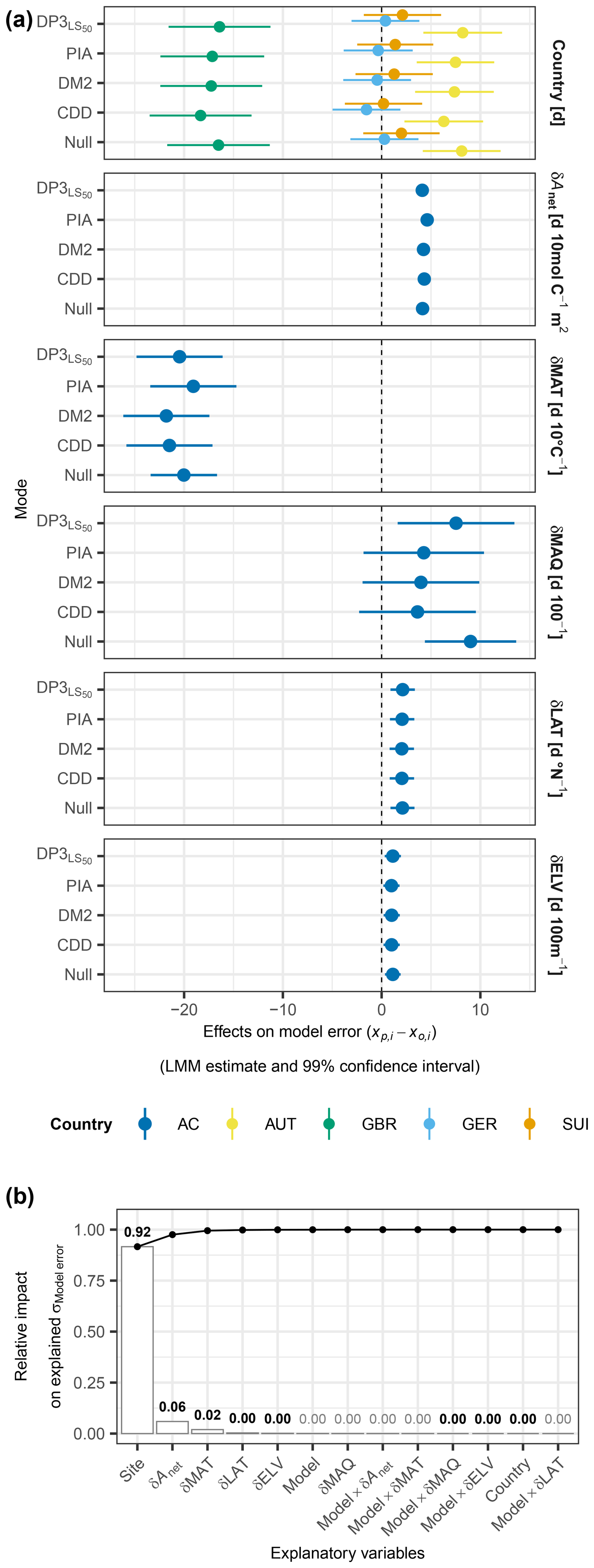
Figure 9 Model error versus data structure and climatic and spatial deviations. Panel (a) visualizes the LMM-based, model-specific estimated fixed effects (dots) and 99 % confidence intervals (bars) of data structure described by “country”, climatic deviations described by mean annual temperature (δMAT; d 10 °C⁻¹), mean annual Keetch and Byram drought index (δMAQ; d 100⁻¹), accumulated net photosynthetic activity between leaf unfolding and summer solstice (δA_net; d 10 mol C⁻¹), and spatial deviations described by latitude (δLAT; d °N⁻¹) and elevation (δELV; d 100 m⁻¹). These deviations were calculated as the difference between a given site year and the average in the calibration sample. The colors indicate the countries Austria (AUT), Great Britain (GBR), Germany (GER), and Switzerland (SUI) as well as estimates across countries (AC). The model error was calculated as the predicted minus the observed timing ($x_{p,i}-x_{o,i}$). Panel (b) shows, based on the ANOVA, the relative impact of the explanatory variables on the variance in the model error as explained by the LMM. The random intercepts in the LMM were grouped by “site”, also describing data structure. The bars indicate the impact of individual variables, while the connected dots show the accumulated impact. The numbers above each bar state the impact, in bold in the case of combined significance and decisiveness (i.e., p≤0.01 and BF${}_{\mathrm{01}}\le \mathrm{1}/\mathrm{1000}$).

4 Discussion

4.1 Model formulation

The DP3 model predicts leaf senescence dates through a novel formulation that differs considerably from the formulation of current models. This novel formulation may change the way we see leaf senescence, i.e., as a consequence of leaf development that relates to both aging and stress. Current models start their simulation with the onset of senescence, i.e., the senescence induction date, which they determine from day length and temperature (e.g., Delpierre et al., 2009; Dufrêne et al., 2005; Keenan and Richardson, 2015; Lang et al., 2019; Liu et al., 2019; Zani et al., 2020). This date is calibrated such that leaf senescence dates are predicted most accurately. In the DP3 model, and in addition to this prerequisite, accumulated aging or accumulated stress since leaf unfolding must have reached a given threshold (i.e., Y_Aging,2 and Y_Stress as well as Fig. 3c and a, respectively; Table 3). In other words, while current models define the senescence induction date backward, the DP3 model defines it both backward and forward, arguably resulting in a more robust definition. Moreover, as current models generally ignore aging (but see the model by Keenan and Richardson, 2015, which considers the leaf unfolding date in the stress threshold for leaf senescence), their formulation partially ignores current knowledge (e.g., Field and Mooney, 1983; Guo et al., 2021; Jibran et al., 2013; Lim et al., 2007). In addition, the models by Liu et al. (2019) and Zani et al. (2020) postulate an effect of the conditions before senescence induction on senescence duration, which remains speculative. However, these conditions likely affect senescence induction dates, possibly through photosynthetic activity (Zohner et al., 2023) or through aging and stress (DP3 model).

The novel formulation of the DP3 model supports the advancement of leaf senescence research by postulating new hypotheses. To our knowledge, it is the first process-based leaf senescence model that (a) predicts leaf senescence dates through daily leaf development status, (b) starts the simulation with leaf unfolding, (c) differentiates between daily aging and stress rates, and (d) predicts the dates of transition between the leaf developmental phases young, mature, and old leaf as well as the senescence induction date. This allows the development of several new hypotheses (Carley, 1999; Hauke et al., 2020), which may relate to the currently disputed effect of climate change on productivity (Lu and Keenan, 2022; Norby, 2021; Zani et al., 2020; Zohner et al., 2023) and can be tested by controlled experiments. In particular, these hypotheses may concern (1) the duration of the young leaf phase during which stress cannot induce senescence, (2) the timing and cause (i.e., aging versus stress) of senescence induction, and (3) the relative importance of the stressors in relationship to climate and location, all of which are further elaborated on here below.

The duration of the young leaf phase differed considerably between the DP3${}_{{\mathrm{LS}}_{\mathrm{50}}{\text{–LS}}_{\mathrm{100}}}$ and DP3${}_{{\mathrm{LS}}_{\mathrm{50}}}$ model (i.e., the DP3 models calibrated with the LS₅₀–LS₁₀₀ versus LS₅₀ samples; Sect. 2.4), i.e., 41 d versus 1 d, respectively. Because the DP3 assumes that stress during this phase is irrelevant for senescence induction, the duration of this phase affects the induction and end of senescence (see below). Moreover, corresponding projections under future climate scenarios are also likely affected, as the probability of late spring frost events will likely change under climate warming (Bigler and Bugmann, 2018; Meier et al., 2018; Sangüesa-Barreda et al., 2021). Therefore, duration and characteristic of this young leaf phase should be examined further, e.g., with controlled experiments that apply continuous stress right after leaf unfolding to determine until when stress is either completely irrelevant for senescence induction or accumulates without inducing senescence.

Senescence was induced in late spring/early summer and more often by stress than by aging, but the induction dates and the stress:aging ratios differed notably between the DP3${}_{{\mathrm{LS}}_{\mathrm{50}}{\text{–LS}}_{\mathrm{100}}}$ and DP3${}_{{\mathrm{LS}}_{\mathrm{50}}}$ model. Senescence induction dates predicted by the DP3${}_{{\mathrm{LS}}_{\mathrm{50}}{\text{–LS}}_{\mathrm{100}}}$ and DP3${}_{{\mathrm{LS}}_{\mathrm{50}}}$ models differed by 40 d, which matches the difference in the predicted duration of the young leaf phase (see above). As stress during the young leaf phase does not affect the predicted leaf senescence dates by definition (Figs. 1, 3a, and c), this result illustrates the importance of studying the effects of stress after leaf unfolding (see above). It also shows that different combinations of calibrated model parameters eventually yield similar predictions. Such compensating effects between different model parameters have also been reported in previous studies (Chuine and Régnière, 2017; Van der Meersch and Chuine, 2025), and explain the different stress:aging ratios as well as the earlier senescence induction during warmer years and at lower elevations. On the one hand, the ratio of stress to aging induced senescence shifts in favor of stress with shorter young leaf phases, because more cold stress can accumulate in spring. On the other hand, senescence must be induced earlier when senescence lengthens to predict leaf senescence dates that are close to the average observation in the calibration sample, as suggested by model accuracy and model error (see below). Longer senescence, in turn, results from arguably reduced cold stress in fall in warmer years and at lower sites. Nevertheless, earlier induction and longer duration of senescence in warmer years may also be a valid description of reality (Zohner et al., 2023). However, Zohner et al. (2023) argue that senescence induction dates relate negatively to pre-solstice productivity (see also Zani et al., 2020), whereas we show that these dates relate to particular interactions between aging and stress rather than to productivity (see below; Eqs. 3 and 10; Lu and Keenan, 2022; Marqués et al., 2023; Norby, 2021). Because such different mechanisms very likely affect leaf senescence projections under climate warming, they certainly need further investigations.

How do aging and stress interact to predict earlier induction and longer duration of senescence in warmer years and at lower sites? The aging requirement for the transition from mature to old leaf (i.e., Y_Aging,2; Table 3) represents the longest possible duration from leaf unfolding to senescence induction. Earlier senescence induction is only possible through sufficient stress between the transition from young to mature leaf and senescence induction (i.e., Y_Stress; Table 3), whereas stress after senescence induction relates negatively to the duration of senescence. Thus, according to the DP3 model, both earlier leaf unfolding and increased stress in spring advance senescence induction, while reduced stress in summer and fall lengthens senescence, which corresponds to observed patterns. Leaves unfold earlier at lower sites in general (Vitasse et al., 2009, 2013) and in warm springs in particular (given that the buds have been sufficiently chilled; Asse et al., 2018; Meier et al., 2021; Menzel et al., 2020). Warmer years have been shown to increase cold stress in spring (i.e., through leaves unfolding overly early in comparison to late frost; Asse et al., 2018; Meier et al., 2018; Sangüesa-Barreda et al., 2021) and relate positively to dry stress (i.e., through evapotranspiration; Allen et al., 1994; Berdanier and Clark, 2018; Wu et al., 2022), but leave photoperiod stress unaffected (Brock, 1981). Thus, earlier senescence induction is likely due to earlier leaf unfolding, and thus aging, and increased cold and dry stress in spring, while the longer senescence duration is likely due to the later accumulation of photoperiod stress relative to leaf development and reduced cold stress in summer and fall.

Surprisingly at first, the DP3${}_{{\mathrm{LS}}_{\mathrm{50}}{\text{–LS}}_{\mathrm{100}}}$ model postulated photoperiod rather than cold and dry stress as being the most important stressor for senescence induction during warmer years, whereas the DP3${}_{{\mathrm{LS}}_{\mathrm{50}}}$ model saw photoperiod stress as being most important during cooler years. By definition, stress only matters when it occurs after the transition from young to mature leaf (Figs. 1, 3a, and c). Photoperiod stress occurs, if at all, after this transition (i.e., after 21 July to 9 September in the DP3${}_{{\mathrm{LS}}_{\mathrm{50}}{\text{–LS}}_{\mathrm{100}}}$ model and after 23–24 June in the DP3${}_{{\mathrm{LS}}_{\mathrm{50}}}$ model, depending on latitude; Table 3) and gains in importance quickly after the first occurrence unless senescence is induced soon by either cold or dry stress. Cold stress likely occurs in spring and fall, both before and after the transition from young to mature leaf. Thus, cold days in spring are less likely to affect senescence induction the later the young leaf phase ends, and vice versa. In addition, more cold days in fall can be accumulated the later the young leaf phase ends and the later photoperiod stress starts to accumulate, and vice versa. Therefore, on the one hand, the long young leaf phase and late accumulation of photoperiod stress in the DP3${}_{{\mathrm{LS}}_{\mathrm{50}}{\text{–LS}}_{\mathrm{100}}}$ model favor the accumulation of cold stress in fall, which arguably decreases in warmer years, making photoperiod stress relatively more important. On the other hand, the short young leaf phase in the DP3${}_{{\mathrm{LS}}_{\mathrm{50}}}$ model favors the accumulation of cold stress in spring, which likely decreases in cooler years through leaves unfolding overly late in comparison to late frost (Asse et al., 2018; Meier et al., 2018; Sangüesa-Barreda et al., 2021), making photoperiod stress relatively more important.

4.2 Model accuracy

We compared the DP3 model to three previous models of leaf senescence (i.e., the models CDD, DM2, and PIA; Delpierre et al., 2009; Dufrêne et al., 2005; Zani et al., 2020) based on the LS₅₀ calibration sample and found the RMSE of all compared models to be above the RMSE for the Null model. This may be explained by unrealistic model formulations, poor model calibrations, and noisy data to drive and calibrate the models, all of which we discuss here below.

While the formulations of the compared models differ, they all build on the results of previous studies. For example, according to all compared models, the leaf senescence date advances due to cold temperatures, which was also observed by Kloos et al. (2024), Wang et al. (2022), Wang and Liu (2023), and Xie et al. (2015, 2018). Moreover, in all but one model, shorter days cause earlier leaf senescence, which is in agreement with Addicott (1968), Keskitalo et al. (2005), Singh et al. (2017), Tan et al. (2023), and Wang et al. (2022). Therefore, while the Null model predicted the leaf senescence dates more accurately according to the RMSE, it is unlikely that it is more realistically formulated than the compared models. The currently most realistic model is arguably the DP3 model (Jan et al., 2019; Jibran et al., 2013; Lim et al., 2007), which makes it the first choice to study the leaf senescence process (see above). Moreover, while the Null model could be a good choice for predictions of leaf senescence dates (i.e., accuracy), the most suited models for predictions of leaf senescence trends (i.e., precision) may have to be identified yet.

We calibrated the compared models with the generalized simulated annealing algorithm and with model-specific controls (Sects. 2.4 and S2.1; Xiang et al., 1997, 2017). Algorithm and controls affect the accuracy of the calibrated models (Meier and Bigler, 2023). Therefore, we used generalized simulated annealing, which was shown to yield accurate models of leaf phenology (Chuine et al., 1998; Meier and Bigler, 2023) and has been used by many studies to calibrate such models (e.g., Basler, 2016; Liu et al., 2019; Meier et al., 2018; Zani et al., 2020). In addition, we used model-specific controls selected to most accurately predict leaf senescence dates for the same validation samples (Sect. S2.2) as the comparison to the Null model was based on. Possible overfitting (James et al., 2017) through this procedure would have benefited the compared models and is unlikely, as the number of observations in the calibration samples was large enough (Sect. 2.4; Jenkins and Quintana-Ascencio, 2020; Meier and Bigler, 2023). Therefore, it is highly improbable that this procedure caused the models to be calibrated so poorly that they are outperformed by the Null model.

All compared models were driven with daily weather data from the E-OBS dataset (Cornes et al., 2018) and calibrated and validated with leaf senescence data from the datasets of MeteoSwiss and PEP725 (Swiss phenology network, 2025; Templ et al., 2018). The E-OBS dataset has been used by many studies (e.g., Bowling et al., 2024; Meng et al., 2021; Schwaab et al., 2021; Zeng and Wolkovich, 2024), and we are unaware of any difficulties concerning the daily weather data used here. The MeteoSwiss and PEP725 datasets, however, compile visually observed leaf senescence data, and such data are noisy due to different observers and small sample sizes (Liu et al., 2021): estimates of the leaf senescence dates for individual trees varied by 15 d (median, spreading from 2 to 53 d) between observers and increased to 28 d (median) for different samples of 10 trees. The data become even noisier if the observers follow different protocols from various institutions and countries (Menzel, 2013), eventually blurring the signal of the leaf senescence process. Arguably, the more this signal is blurred, the closer the simulations will follow the mean observation in the data. Here, we used leaf senescence data from 244 sites (i.e., probably at least 244 observers) and four countries (Sect. 2.1), which implies considerable noise and thus a blurred signal of the leaf development process. These data very likely forced the compared models to predict leaf senescence dates close to the mean observation, impairing their accuracy.

4.3 Model error

While climatic and spatial deviations from the calibration sample generally affected the model error, their model-specific effects only differed insignificantly from the Null model. In other words, the model error in the compared models reacted similarly to climatic and spatial deviations as the model error of the Null model. This implies that the compared models predicted leaf senescence dates closely to the mean observation of the calibration sample and thus were heavily biased to the mean (i.e., as the Null model). Possible explanations for this are unrealistic model formulations, poor model calibrations, and noisy data. Interestingly, Meier et al. (2023), who reported a heavy bias towards the mean for 21 process-oriented models of leaf senescence, based their study on leaf senescence data from 500 sites (i.e., probably at least 500 observers) and at least three countries from the PEP725 dataset (Templ et al., 2018). This supports our inference that the compared models resorted to the mean observation due to the used leaf senescence data rather than to model formulations and model calibrations.

Moreover, leaf senescence data were most relevant for the model error in the compared models, which was illustrated by the fixed effects of countries and the variation caused by the random intercepts grouped by sites. These effects of countries differed considerably between countries, demonstrating how different observation protocols (see above; Menzel, 2013) add noise to leaf senescence data, which to our knowledge has not yet been investigated. The random intercepts grouped by sites varied considerably, and corresponding differences among sites were attributed to a substantial amount of the explained variance in the model error (chap. 23.3.2 in Fox, 2016). Meier et al. (2023) also noted a large amount of the explained variance in the RMSE being attributed to differences between the sites. They reasoned that this was caused by, among others, noisy leaf senescence data (see above) and different interannual variability of observations between the sites (Cole and Sheldon, 2017; Čufar et al., 2015; Li et al., 2022; Liu et al., 2020). It remains to be seen if such site-specific interannual variability as well as inter-site variability in leaf senescence dates would be predicted correctly by models calibrated with noise-free data.

4.4 Ways forward

While the DP3 model is likely the currently most realistic process-oriented model of leaf senescence, it may be developed further by (1) testing other drought indices, (2) considering nutrient depletion in combination with drought, and (3) ameliorating the formulation of the senescence rate. First, while various indices summarize drought differently (Speich, 2019; Zargar et al., 2011), the KBDI used here can be calculated from few data, being based on precipitation and temperature. It should be tested, however, if other indices, such as the standardized precipitation evapotranspiration index (based on precipitation and temperature; Vicente-Serrano et al., 2010) or the ratio of actual to potential evapotranspiration (based on precipitation, temperature, and soil moisture; Bugmann and Cramer, 1998), may approximate the effects of dry stress on leaf senescence more accurately. Second, despite more accurate predictions of LS₅₀ and LS₁₀₀ when nutrient depletion was disregarded (Figs. 6 and S1), model errors indicated that LS₅₀ and LS₁₀₀ dates were predicted later than observed due to nutrient depletion as approximated by elevation (Fig. 9; Tables S9–S10). This can be explained by higher elevation relating to increased nutrient depletion, which in turn fuels dry stress (Fu et al., 2014; Huber et al., 2007; Loomis et al., 2006; Tan et al., 2023). Consequently, drought indices that consider nutrient depletion should be tested. Third, the DP3${}_{{\mathrm{LS}}_{\mathrm{50}}{\text{–LS}}_{\mathrm{100}}}$ model was considerably less accurate than the DP3${}_{{\mathrm{LS}}_{\mathrm{50}}}$ model, implying difficulties in the accurate, simultaneous prediction of LS₅₀ and LS₁₀₀. This points to an incorrectly formulated dependency of the senescence rate on aging and stress (Eqs. 1 and 12), and corresponding new formulations should be evaluated.

In addition, because noisy data blur the signal of the leaf development process, (1) alternative data may be used, (2) observation protocols may be revised, and (3) visually observed data may be carefully selected. First, alternative data to calibrate and validate models of leaf senescence include data recorded with phenocams and remotely sensed data in which leaf senescence dates are identified through the measured greenness, machine learning algorithms, and vegetation indices (Donnelly et al., 2022; Dronova and Taddeo, 2022; Gong et al., 2024; Richardson, 2023; Zeng et al., 2020). While these data are species-specific if recorded with phenocams, this may not be the case for remotely sensed data (Joiner et al., 2016; Tang et al., 2016). Second, revised observation protocols should describe how to determine dates of leaf senescence stages (i.e., senescence induction, LS₅₀, and LS₁₀₀ at least) based on the measured, rather than estimated, state of leaf senescence. Such a measurement could be based on the greenness derived from images taken with consumer-grade digital cameras (Ide and Oguma, 2013; Richardson et al., 2018; Toomey et al., 2015; Zimmerman and Richardson, 2024). Moreover, a given observational time series should be based on at least 25 trees which are measured every other week (Liu et al., 2021; Morellato et al., 2010). Third, visually observed leaf senescence data should be selected primarily from the point of view of precision, e.g., by ensuring identical observation protocols and by sampling from cleaned data with a minimum of breakpoints (i.e., sudden changes in the mean). For this, the time series may be cleaned from outliers (Schaber et al., 2010) and separated through a breakpoint analysis (Auchmann et al., 2018) before being sampled, preferably through spatially and climatologically stratified sampling, according to the research focus (e.g., gaining insight into the underlying processes or producing most accurate or most precise predictions; Meier and Bigler, 2023).

5 Conclusion

The DP3 model builds on three subsequent phases of leaf development: the young, mature, and old leaf phase. The young leaf is insensitive to stress and transfers into a mature leaf solely due to aging. The mature leaf answers to aging and stress, both of which may induce senescence. While aging induces senescence with the transition from mature to old leaf, stress may already do so during the mature leaf phase through combining cold stress, photoperiod stress, and dry stress. The output of the DP3 model includes daily rates of aging rates as well as of cold, photoperiod, and dry stress, along with the dates of transition from young to mature to old leaf, senescence induction dates, and the leaf senescence dates. Thus, the DP3 model allows to develop testable hypotheses about the leaf senescence process, e.g., regarding the effect of site conditions on the induction and duration of senescence: the DP3 model predicted earlier onset of senescence (i.e., senescence induction) under warmer conditions, likely due to earlier leaf unfolding and thus aging, and increased cold and drought stress in spring, as well as longer-lasting senescence, likely due to the later accumulation of photoperiod stress relative to leaf development and reduced cold stress in summer and fall. Both these predictions and their implied relationships with aging and stress can be tested through experiments and in situ observations. This makes the DP3 model an important tool in the research of leaf senescence.

The accuracy of the DP3 model and of previous models of leaf senescence was lower than the accuracy of the Null model (i.e., the constant prediction of the average observation in the calibration sample). This was probably due to model formulations that do not fully reflect the leaf senescence process and, more importantly, to the leaf senescence data used for calibration and validation. Visually observed leaf senescence data are susceptible to observer bias and based on observation protocols that are partly inconsistent between countries. Such noisy data blur the signal of the leaf senescence process, thereby probably forcing the models to resort to the average observation. This leads to low accuracy, regardless of the model formulation, which hinders the necessary further development of process-oriented models of leaf senescence.

The model error of the compared models was similarly affected by climatic and spatial deviations from the calibration sample across models, and varied mainly due to the leaf senescence data. The similar effect of climatic and spatial deviations on the model error across models (including the Null model) illustrates that these models were heavily biased towards the mean. Moreover, the degree of noise in the used leaf senescence data is exemplified by these data accounting for over 90 % of the explained variance in the model error. Therefore, these data should be selected with particular attention to precision, e.g., by using time series without sudden changes in the mean. Moreover, revised observation protocols should include senescence induction dates and rely on measurements rather than visual estimates. Such measurements may be based on the greenness of leaves to identify the degree of color change, involving digital cameras and automated image assessment.