Design, evaluation, and future projections of the NARCliM2.0 CORDEX-CMIP6 Australasia regional climate ensemble

NARCliM2.0 (New South Wales and Australian Regional Climate Modelling) comprises two Weather Research and Forecasting (WRF) regional climate models (RCMs) which downscale five Coupled Model Intercomparison Project Phase 6 (CMIP6) global climate models contributing to the Coordinated Regional Downscaling Experiment (CORDEX) over Australasia at 20 km resolution and southeast Australia at 4 km convection-permitting resolution. We first describe NARCliM2.0's design, including selecting two definitive RCMs via testing 78 RCMs using different parameterisations for the planetary boundary layer, microphysics, cumulus, radiation, and land surface model (LSM). We then assess NARCliM2.0's skill in simulating the historical climate versus CMIP3-forced NARCliM1.0 and CMIP5-forced NARCliM1.5 RCMs and compare differences in future climate projections. RCMs using the new Noah multi-parameterisation (Noah-MP) LSM in WRF with default settings confer substantial improvements in simulating temperature variables versus RCMs using Noah Unified. Noah-MP confers smaller improvements in simulating precipitation, except for large improvements over Australia's southeast coast. Activating Noah-MP's dynamic vegetation cover and/or runoff options primarily improves the simulation of minimum temperature. NARCliM2.0 confers large reductions in maximum temperature bias versus NARCliM1.0 and 1.5 (1.x), with small absolute biases of ∼ 0.5 K over many regions versus over ∼ 2 K for NARCliM1.x. NARCliM2.0 reduces wet biases versus NARCliM1.x by as much as 50 % but retains dry biases over Australia's north. NARCliM2.0 is biased warmer for minimum temperature versus NARCliM1.5, which is partly inherited from stronger warm biases in CMIP6 versus CMIP5 GCMs. Under Shared Socioeconomic Pathway (SSP) 3-7.0, NARCliM2.0 projects ∼ 3 K warming by 2060–2079 over inland regions versus ∼ 2.5 K over coastal regions. NARCliM2.0-SSP3-7.0 projects dry futures over most of Australia, except for wet futures over Australia's north and parts of western Australia, which are the largest in summer. NARCliM2.0-SSP1-2.6 projects dry changes over Australia with only few exceptions. NARCliM2.0 is a valuable resource for assessing climate change impacts on societies and natural systems and informing resilience planning by reducing model biases versus earlier NARCliM generations and providing more up-to-date future climate projections utilising CMIP6.

1 Introduction

Climate projections are foundational to informing climate change mitigation and adaptation planning at various spatial scales (IPCC, 2021). Regional climate models (RCMs) dynamically downscale global climate models (GCMs) at ∼ 100–200 km resolution to simulate higher-resolution climate projections that better resolve local-scale influences on regional climate, such as mountain ranges, land-use variation, land–sea contrasts, and convective processes (Torma et al., 2015; Giorgi, 2019). As such, whilst GCMs are the best tools for investigating climate at global scales, RCMs provide improved guidance for climate policy at the regional scale, which is the scale at which climate change impacts are experienced (Hsiang et al., 2017).

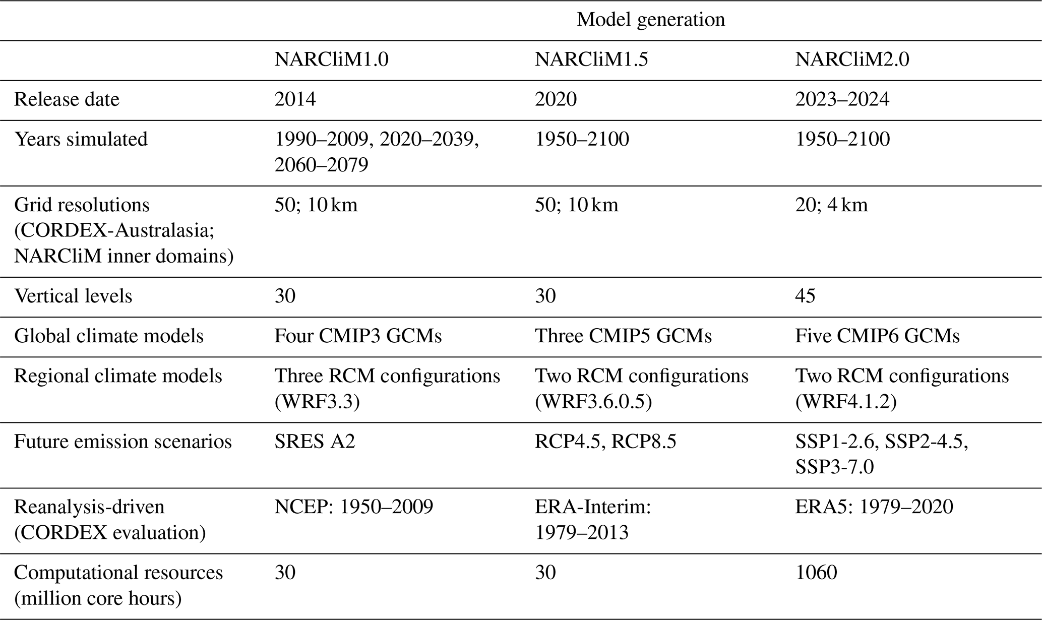
The NARCliM (New South Wales and Australian Regional Climate Modelling) programme is now in its third generation. Like its predecessors, NARCliM version 2.0 (NARCliM2.0) aims to produce robust, detailed regional climate projections at spatial scales relevant for use in local-scale climate change analysis. A key feature of all NARCliM generations is to simulate the climate over the Coordinated Regional Downscaling Experiment (CORDEX) Australasia domain and a higher-resolution inner domain over southeast Australia via one-way nesting (Fig. 1). With one-way nesting, the inner domain obtains its initial and lateral boundary conditions from the simulation over CORDEX-Australasia. NARCliM1.0 simulated the climate of Australasia for three periods (1990–2009, 2020–2039, and 2060–2079) at 50 km resolution and southeast Australia at 10 km using three configurations of the weather research and forecasting (WRF) RCM (Skamarock et al., 2008) to downscale GCMs from the Coupled Model Intercomparison Project Phase 3 (CMIP3) under the greenhouse gas (GHG) Special Report on Emissions Scenario (SRES) A2 (Evans et al., 2014). NARCliM1.5 used CMIP5 GCMs under Representative Concentration Pathways (RCP) 4.5 and 8.5 to simulate continuously for 1950–2100 on the same grids as NARCliM1.0 using two of its RCMs (Nishant et al., 2021).

NARCliM2.0 aims to improve performance in simulating the Australian climate relative to previous NARCliM generations with the goal of better informing community resilience to climate change (NSW Government, 2022, 2023). All NARCliM projects include a bottom-up design ethos involving multi-sectoral end-user engagement in specifying model requirements to ensure model performance and outputs meet end-user needs. Key requirements from the NARCliM2.0 user consultation include providing increased detail in climate simulations via higher resolution and improving the simulation of precipitation and temperature as these are fundamental inputs to climate impact studies. Whilst NARCliM1.0 and 1.5 (1.x) confer the expected level of performance in simulating the Australian climate (Di Virgilio et al., 2019; J. P. Evans et al., 2020), recent technological and scientific advancements mean that aspects of their performance might now be improved. NARCliM1.x RCMs show widespread cold biases in maximum temperature exceeding −5 K for some RCMs. Conversely, minimum temperature is simulated more accurately with biases in the range of ±1.5 K. NARCliM1.x RCMs overestimate precipitation, particularly over Australia's socioeconomically important eastern seaboard (Di Virgilio et al., 2019).

As they are expensive to run from both computational and data storage perspectives, dynamical downscaling projects like NARCliM2.0 use a subset of available GCMs as driving data, necessitating careful model selection. Similarly, a large combination of different physical parameterisations available for the WRF RCM enables many structurally different RCMs to be potentially used to downscale GCMs. A key component of NARCliM2.0's design is testing the viability of alternative RCM parameterisations via a three-phase approach, with each phase building on the preceding phase to identify the RCM parameterisations that perform well during testing to meet NARCliM2.0's aim of improving the simulation of Australia's climate. GCM and RCM statistical independence is also sought to avoid creating a biased sample of climate change. Hence, the aims of this paper are to

1. describe how and why NARCliM2.0 differs from its predecessors in terms of its design and production processes, explaining the model test and evaluation approaches underlying its design decisions, where a key focus is on the design and testing of 78 structurally different WRF RCMs and their evaluation to identify a subset of RCMs for use in NARCliM2.0;

2. characterise the performance improvements of CMIP6-NARCliM2.0 RCMs in simulating the Australian climate relative to previous NARCliM generations by evaluating their skill in simulating mean maximum and minimum temperature and precipitation versus observations;

3. summarise the climate projections produced by CMIP6-NARCliM2.0 and how these differ from previous CMIP3-5-NARCliM generations.

The following section summarises the basic design features of each NARCliM generation. Section 3 describes evaluation methods and metrics, Sect. 4 describes NARCliM2.0's design process with a focus on its RCM physics testing as well as a brief overview of its production process, Sect. 5 summarises the RCM physics test results, Sect. 6 evaluates the performance of all NARCliM models in simulating the recent Australian climate, Sect. 7 provides an overview of their future projections, Sect. 8 discusses key results, and Sect. 9 summarises this paper.

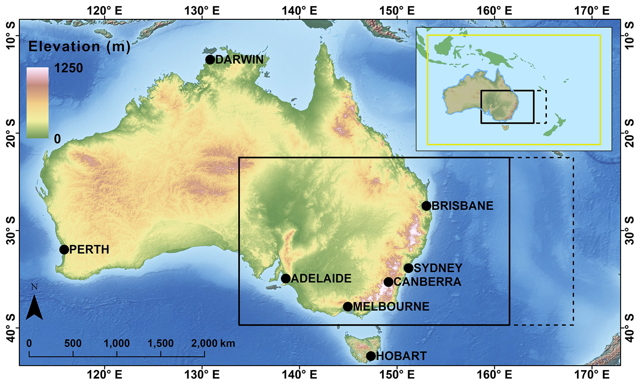
Figure 1 Model domains for NARCliM regional climate simulations. The southeast inner domain for NARCliM2.0 is delineated with a solid black rectangle; the corresponding inner domain for NARCliM1.0 and 1.5 is delineated with a dashed black line. The elevated terrain of the Australian Alps, which form part of the Great Dividing Range, is in eastern Australia. The inset shows the CORDEX-Australasia outer domain.

2 Three generations of NARCliM: model overviews

The design of NARCliM1.0 is described in Evans et al. (2014); NARCliM1.5 used the same design approach but used CMIP5 rather than CMIP3 GCMs. All generations of NARCliM use different versions of the WRF model to perform dynamical downscaling of GCMs since the WRF model goes through regular updates. The southeast Australian inner domain captures five of Australia's eight capital cities (Fig. 1) and over 75 % of the Australian population (Australian Bureau Statistics, 2024). Additionally, the inner domain captures coastal regions that are characterised by topographic complexity and land-use class variation. Regions east of the Great Dividing Range mountains in southeast Australia (Fig. 1) show different responses to oceanic climate modes compared to inland semi-arid regions (Murphy and Timbal, 2008) and are impacted by events such as rapidly developing storms, including east-coast lows (Pepler and Dowdy, 2021). Such atmospheric processes are not adequately resolved by GCMs due to coarse resolutions (Di Virgilio et al., 2022; Grose et al., 2020).

NARCliM2.0 encompasses several design advancements over its predecessors (Table 1). NARCliM2.0 RCMs have a 20 km resolution CORDEX-Australasia domain (versus 50 km) and a 4 km (versus 10 km) domain over southeast Australia and use 45 (versus 30) vertical levels. The aim of increasing the resolution of this inner domain from 10 to 4 km is to render these simulations convection-permitting (Kendon et al., 2021; Lucas-Picher et al., 2021). Hence, whilst the 20 km resolution outer domain uses cumulus parameterisation, simulations over the 4 km domain do not use cumulus parameterisation. NARCliM2.0 also includes a new collaboration with the Western Australian government, with separate 4 km simulations being performed over southwest and northwest Western Australia (not shown in Fig. 1) as part of the Western Australian climate science initiative (DWER, 2023). Boundary conditions derived from the 20 km NARCliM2.0 CORDEX-Australasia domain are used to drive these simulations. Additional major differences in model setup for NARCliM2.0 include

• NARCliM1.0 RCMs use different parameterisations for planetary boundary-layer (PBL) physics, surface physics, cumulus physics, land surface model (LSM), and radiation (Evans et al., 2014). These RCM parameterisations were also used for NARCliM1.5. Owing to the project aims stated above, RCM parameterisations for NARCliM2.0 differ from those of NARCliM1.x (see Sect. 4).

• NARCliM2.0 increases the number of driving GCMs to five and simulates for a wider range of plausible future climates via three Shared Socioeconomic Pathways (SSPs). SSP1-2.6 is selected as a low-GHG scenario envisaging a future climate with CO₂ emissions cut to net zero by around 2075 and warming held to below 2 °C by 2100, SSP2-4.5 estimates projected warming under a middle-of-the-road scenario where temperatures increase to ∼ 2.7 °C by 2100, and SSP3-7.0 is a high-GHG scenario which assumes a warming of ∼ 4 °C by 2100 (IPCC, 2021).

• Urban physics is activated in NARCliM2.0 (WRF setting: sf_urban_physics = 1) to represent surface energy balance in urban areas via a single-layer urban canopy model (Kusaka and Kimura, 2004).

• Input of different aerosol species is activated for the RCM radiation scheme using the Tegen et al. (1997) climatology available in WRF (aer_opt = 1). This aerosol forcing is the same for all GCMs and is not model-specific.

• The eastern boundary of the NARCliM2.0 inner domain is located further westward relative to that of NARCliM1.x (Fig. 1).

Table 1 High-level design features of three generations of NARCliM regional climate models.

3 Evaluation methods

This section largely focuses on the methods and metrics used for the NARCliM2.0 RCM physics testing and comparisons of model biases and future climate projections with previous generations of NARCliM. Details on methods and results for the CMIP6 GCM evaluation used to select driving GCMs and the ERA5-NARCliM2.0 RCM evaluation used to select two definitive RCMs for the GCM-driven simulations are available in Di Virgilio et al. (2022) and Di Virgilio et al. (2025), respectively, with overviews of these components of NARCliM2.0 design provided in Sect. 4.2 and 4.4 below.

3.1 Observations

Australian Gridded Climate Data (AGCD version 1.0; A. Evans et al., 2020) are the observational data used to evaluate the NARCliM2.0 RCM physics test RCMs. These daily gridded data for maximum and minimum temperature and precipitation are obtained from an interpolation of station observations across Australia. AGCD data are on a regular WGS84 grid with a grid-averaged resolution of 0.05°. For the NARCliM2.0 RCM physics tests, the AGCD data were re-gridded to correspond to the RCM data from the inner domain on their native grids using a conservative area-weighted re-gridding scheme. All data (RCM and AGCD) were restricted to a common extent contained within the inner domain over southeast Australia, and a land mask was applied so that statistics were computed using only land pixels. Treatment of AGCD for the CMIP6 GCM evaluation and the ERA5-NARCliM2.0 RCM evaluation is described in Di Virgilio et al. (2022) and Di Virgilio et al. (2025), respectively.

3.2 Methods and metrics: phase I–III NARCliM2.0 physics tests

Test RCM performances in reproducing observations for daily maximum and minimum temperature and daily precipitation were assessed by calculating the model bias, i.e. model outputs without AGCD, and the root mean squared error (RMSE) of modelled versus observed fields. Model biases and RMSEs were calculated at annual and seasonal timescales. The model representations of the hottest and the wettest day on an annual timescale over the study region were also compared with AGCD. Probability density functions (PDFs) were calculated for each variable using daily data. Perkins' skill score (PSS) (Perkins et al., 2007) was calculated to assess the overall degree of overlap between modelled and observed distributions, with PSS = 1 indicating that distributions overlap perfectly.

There are several methods to evaluate the overall performance of RCMs. In this study, we ranked the RCMs individually based on their bias, RMSE, and PSS for maximum temperature, minimum temperature, and precipitation. Each variable was ranked separately for each metric. The ranks were then summed to determine the overall ranking for each RCM.

3.3 Independence assessments

We used the method of Bishop and Abramowitz (2013) as one of two methods of assessing the independence of physics test RCMs and the target CMIP6 GCMs under evaluation for use in NARCliM2.0. This approach uses the covariance in model errors as the basis to define model dependence; specifically, independence coefficients are derived from the error covariance matrix of the RCMs or GCMs. Model independence is quantified using the correlation of model errors. For the physics test RCMs, errors are computed by comparing the climatology of maximum and minimum temperature and precipitation over the southeast Australia inner domain for 2016 with corresponding AGCD observations. The same calculation is performed for the CMIP6 GCMs, except for the Australian continent. Daily time series of precipitation and maximum and minimum temperatures are calculated individually for each RCM and for AGCD. The simulated and observed daily time series of each variable are then normalised by the standard deviation of the corresponding observed variable. These normalised variables are concatenated for each RCM (GCM) and AGCD. An anomaly time series for each grid cell is then produced. These time series are used to create a model error covariance matrix containing the errors for all RCMs (GCMs). The coefficients of a linear combination of the RCMs (GCMs) that optimally minimises the mean square error (MSE) depend on both model performance and model dependence (Bishop and Abramowitz, 2013). The result of this minimisation problem is written in terms of the covariance matrix. The magnitude of coefficients assigned to each RCM (GCM) reflects a combination of their performance and independence. Highly independent models have different errors when simulating the recent climate. Models with the largest coefficients have the most independent errors compared to observations.

The Herger method of subset selection (Herger et al., 2018), as implemented here, uses quadratic integer programming to find the subset of models whose equally weighted subset mean (EWSM) minimises a quadratic cost function. This cost function is chosen to measure the performance of the EWSM in comparison to a given observational product. The two cost functions used here are the mean squared error (MSE) between the EWSM and the observational product (Eq. 1 in Herger et al., 2018) and another which measures a combination of the MSE of the EWSM, the average MSE of each subset member, and the average pairwise mean squared distance between subset members (Eq. 2 in Herger et al., 2018).

3.4 NARCliM2 CMIP6 RCMs: historical evaluation and climate change projections

Performances of NARCliM2.0 versus NARCliM1.x RCMs in reproducing the recent Australian climate are evaluated by calculating the model biases (model outputs without AGCD observations) for mean maximum and minimum temperature and precipitation for 1990–2009. To enable comparison of future projections between NARCliM1.0, NARCliM1.5, and NARCliM2.0 (where NARCliM1.0 projected for 1990–2009, 2020–2039, and 2060–2079), all NARCliM ensemble projected changes are shown as the far future (2060–2079) with the present day (1990–2009) subtracted.

3.5 Statistical significance

When quantifying RCMs' future climate change projections (compared to the historical period) and biases in maximum and minimum temperature, the statistical significance is calculated for each grid cell using t tests assuming equal variance. The Mann–Whitney U test is used for precipitation given its non-normality. Significance thresholds were adjusted to account for multiple testing using Walker's test (Eq. 2 in Wilks, 2016). For individual RCMs, grid cells showing statistically significant changes are stippled; otherwise, they are shown in colour where change is statistically insignificant. Results of the statistical significance of each ensemble mean are separated into three categories following Tebaldi et al. (2011): (1) statistically insignificant areas are shown in colour, denoting that less than 50 % of RCMs are significantly biased/different; (2) in areas of significant agreement (stippled), at least 50 % of RCMs are significantly biased/different, and at least 70 % of significant models in the CMIP6-NARCliM2.0 RCM ensemble agree on the sign of the bias/difference. In such areas, many ensemble members have the same bias sign which is an undesirable outcome; and (3) areas of significant disagreement, where at least 50 % of RCMs are significantly biased/different and fewer than 70 % of significant models agree on the bias sign, are shown with diagonal hatching for the CMIP6-NARCliM2.0 historical evaluation and climate change signals.

4 NARCliM2.0 design and production process overview

The NARCliM2.0 design and production processes are summarised below in reference to Fig. 2. The design process is an adaptation of that introduced in Evans et al. (2014). Two companion manuscripts describe elements shown in Fig. 2, which are therefore only summarised briefly in this manuscript. Di Virgilio et al. (2022) describe the CMIP6 GCM selection process summarised in Box 2, and Di Virgilio et al. (2025) describe the ERA5 RCM evaluation undertaken in Boxes 5 and 6.

• I.

  The design phase comprises the following steps:

  • i.

    Box 1. Model design requirements are identified via consultation between NARCliM2.0 modelling groups and multi-sectoral end users as well as adherence to CORDEX-CMIP6 design requirements (WCRP, 2020).

  • ii.

    Box 2. NARCliM1.x driving CMIP3-5 GCMs (respectively) via literature review of existing GCM evaluations is selected. During NARCliM2.0 design, there were no pre-existing comprehensive evaluations of individual CMIP6 GCMs for the Australian region, including assessments of climate change signals and GCM statistical independence. Hence, an evaluation and selection of CMIP6 GCMs was conducted (see Di Virgilio et al., 2022). This evaluation selected five GCMs to force two NARCliM2.0 RCMs (see Sect. 4.2 and 4.4). The relative contribution to uncertainty/variation in climate projections can be larger for GCMs than for RCMs (e.g. Lee et al., 2023).

  • iii.

    Boxes 3–4. A new WRF RCM multi-physics test ensemble is created for NARCliM2.0: RCM physics testing is conducted via a three-phase approach, with each phase building on the findings of the preceding phase to identify the RCM parameterisations that perform well during testing with the aim of improving the simulation of the Australian climate. In this way, RCMs are parameterised with different physics settings via each test phase, systematically removing poor-performing options while facilitating the fine-tuning and improvement of the parameterisations that perform well during testing to build a total ensemble size of 78 structurally different test RCMs. The performance of the different test RCM configurations is evaluated, ultimately leading to the selection of a subset of seven RCMs for a subsequent downscaling of ERA5 reanalysis as part of the CORDEX evaluation experiment.

  • iv.

    Boxes 5–6. These seven RCMs are used to downscale ERA5 reanalysis over the 20 and 4 km domains for 1979–2020. Evaluating these ERA5-forced simulations informs the selection of two definitive production RCMs for CMIP6-forced downscaling (see Sect. 4.4 and Di Virgilio et al., 2025).

• II.

  The production phase is structured as follows:

  • i.

    Boxes 7–8. CMIP6 GCM data are pre-processed to create initial and boundary conditions to drive simulations for the historical (1950–2014) and SSP experiments (2015–2100). A code repository used for this GCM pre-processing is available on Zenodo at https://doi.org/10.5281/zenodo.11184830 (Di Virgilio et al., 2024) within the WRF/repo_snapshots subdirectory. Quality assurance/quality control (QA/QC) is performed on these data before initiating the simulations (e.g. variables are checked to confirm data do not contain significant outliers across ensemble members).

  • ii.

    Boxes 9–11. The 151-year CMIP6-forced NARCliM2.0 RCM simulations are run using the National Computational Infrastructure at Canberra, Australia (NCI, https://nci.org.au/, last access: 12 December 2024). File integrity verification and QA/QC are performed on each year of raw WRF output throughout the simulation life cycle and prior to post-processing to CORDEX-compliant-format climate variables. QA/QC tests include calculating the minimum, maximum, mean, and standard deviation for key variables over consecutive periods of 6 simulation days. Variables are categorised as either normally distributed or otherwise. Normally distributed variables (e.g. surface temperature) are deemed potentially erroneous if their minima/maxima are more than 5 standard deviations away from the global mean of the relevant statistic of the rolling 6 d period. Non-normally distributed variables (e.g. snow depth and precipitation) are checked only for global minima and maxima.

  • iii.

    Boxes 12–13. After each year of simulation raw output is generated for, their post-processing is initiated to produce CORDEX CORE Tier 1 and Tier 2 variables (WCRP, 2022). A statistical QA/QC process is automatically applied to each year of post-processed CORDEX CORE variables as they are generated throughout the simulations. QA/QC tests include

    • –

      checking for presence of missing values,

    • –

      checking that all values are within realistic ranges for minima and maxima,

    • –

      checking minima and maxima are not equal at any time step with exceptions (e.g. snow depth, which can be zero everywhere in the outer domain),

    • –

      checking that changes over time are within realistic ranges (i.e. assessing temporal gradients),

    • –

      checking that changes between neighbouring data points are within realistic ranges (i.e. assessing spatial gradients),

    • –

      checking the number of grid cells with NaN (non-numerical) values does not exceed the threshold set for the variable.

    Reasonable ranges for variables are determined using a series of threshold values that are based on historical records and/or empirical analysis. QA/QC computer scripts generate exceedance files which output every data point that surpasses the threshold values, and these exceedance files are then manually reviewed to determine whether an issue is a true or false positive and so on.

  • iv.

    Box 14. Once each year of WRF raw files is post-processed, raw files are transferred to a tape facility for long-term storage.

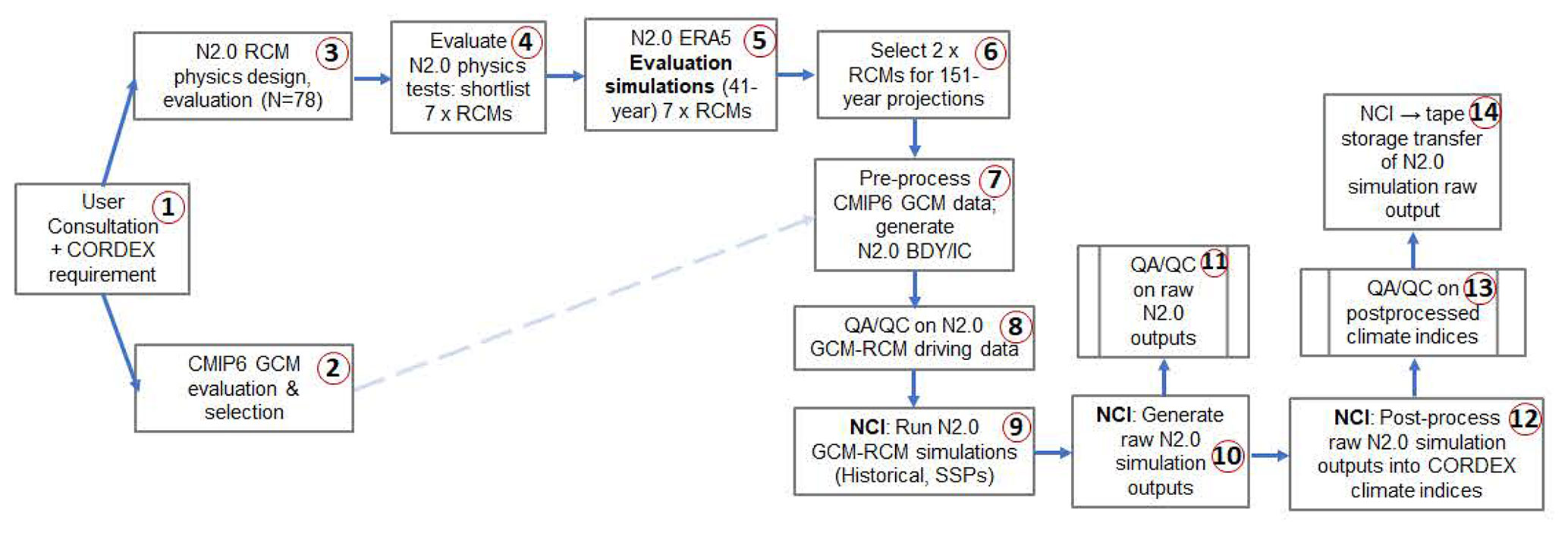
Figure 2 Simplified overview of NARCliM2.0 (N2.0) design and production processes. ERA5: ECMWF Reanalysis v5 data, BDY: boundary conditions, IC: initial conditions, QA/QC: quality assurance/quality control, and NCI: National Computational Infrastructure (high-performance computer used to run N2.0 simulations).

These model design and production stages are now described in more detail.

4.1 Model evaluation and selection

Practical constraints such as available computing and data storage resources enforce an upper limit on GCM–RCM ensemble size. Thus, NARCliM2.0 uses a subset of available CMIP6 GCMs and WRF RCM configurations, necessitating careful GCM and RCM selection to create a subset of GCM–RCMs that provide robust climate simulations whilst also adequately sampling model uncertainty. In selecting a subset of GCMs and RCMs for dynamical downscaling, it is desirable to reject models that perform consistently poorly relative to their peers in simulating the current climate as this provides lower confidence in the projected change (J. P. Evans et al., 2020; Di Virgilio et al., 2022; Grose et al., 2023). Furthermore, the modelled climate space sampled is reduced when selecting a subset of GCMs, which can create a biased view of the climate as well as the plausible change in climate. Care must therefore be taken to ensure that the subset of models used for downscaling is representative of the full range of possible climates and that model errors are uncorrelated, i.e. that models are statistically independent. The steps taken to evaluate and select GCMs and RCMs for NARCliM2.0 are described next.

4.2 CMIP6 GCM evaluation

A three-phase process was used to evaluate individual CMIP6 GCMs (for further details, see Di Virgilio et al., 2022).

4.2.1 CMIP6 GCM performance

We evaluated the performances of individual CMIP6 GCMs in simulating the following aspects of the observed historical climate of Australia:

• annual and seasonal climatologies and daily distributions of maximum and minimum temperatures and precipitation;

• climate extremes, such as the 99th percentiles of daily maximum temperature and precipitation and the 1st percentile of minimum temperature;

• teleconnections of oceanic climate modes and Australian regional rainfall.

Temperature and precipitation variables are chosen for evaluation because, being well-represented in high-quality gridded observational datasets for the Australian continent, they provide the most direct comparison to observations (King et al., 2013). They are also often prioritised for impact studies. Given that variables such as winds (U, V), air temperature (T), water mixing ratio (Q), geopotential height (Z), sea surface temperature (SST), and sea level pressure (PSL) serve as boundary conditions for driving RCMs, these could be incorporated into future GCM evaluation studies. However, evaluating such variables would require the use of reanalysis data as surrogate observations.

A set of GCMs that performed consistently poorly across the variables and statistics considered was identified. These models, as well as those with insufficient data to enable dynamical downscaling using the WRF RCM, were excluded from further evaluation, leaving 27 GCMs for subsequent assessment.

4.2.2 CMIP6 GCM independence

The retained 27 GCMs were subjected to the Bishop and Abramowitz (2013) and Herger et al. (2018) independence analyses (see Sect. 3.5). The GCMs were then ranked according to their relative level of statistical independence.

4.2.3 Sampling CMIP6 GCM climate change spread

For climate change risk assessments, climate projections should reflect as much of the range of plausible future climate changes as possible (Whetton and Hennessy, 2010). The subset of CMIP6 GCMs selected for NARCliM2.0 spanned a wide range of future changes in annual mean temperature and precipitation. Climate change signals were calculated for 2080–2099, omitting 1995–2014, for the Australian continent and southeast Australia under SSP3-7.0 (for the latter, see Fig. 3). The GCM independence rankings were placed within this climate change space, with higher independence rankings viewed as favourable, along with the consideration of the following criteria:

• I.

  A balanced range of GCM equilibrium climate sensitivities (ECSs) were sampled. ECS is the long-term increase in global mean surface air temperature in response to the radiative forcing caused by a doubling of pre-industrial CO₂ concentrations. ECS is related to global temperature change and not just changes over Australia; however, it correlates strongly with regional warming. Around one-third of CMIP6 GCMs show ECS values higher than the upper end of the likely range of 2.5 to 4 °C (IPCC, 2021). An upper range of more than ∼5 °C cannot be ruled out (Meehl et al., 2020; Bjordal et al., 2020; Sherwood et al., 2020).

• II.

  Some CMIP6 GCMs that are favourable in terms of model performance and independence could not be selected as input to WRF for NARCliM2.0 owing to insufficient data availability for key variables, where, ideally, WRF requires subdaily data for the variables shown in Table S1 in the Supplement.

As a result of the above process, the five CMIP6 GCMs listed in Table 2 are selected to force each of the two definitive NARCliM2.0 RCMs selected via the RCM physics testing and ERA5 evaluation processes.

Table 2 Basic details of the CMIP6 GCMs used to force the two definitive RCMs comprising the NARCliM2.0 CORDEX-CMIP6 ensemble.

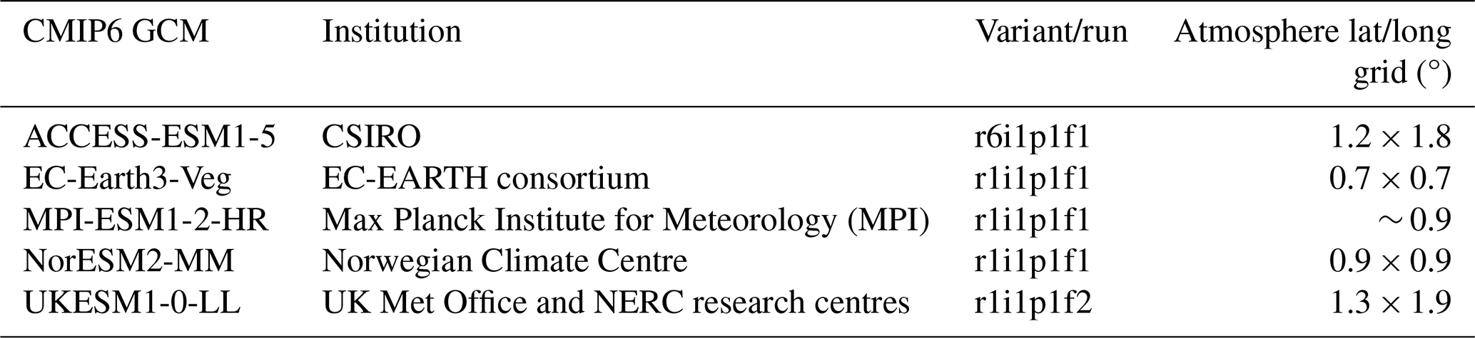
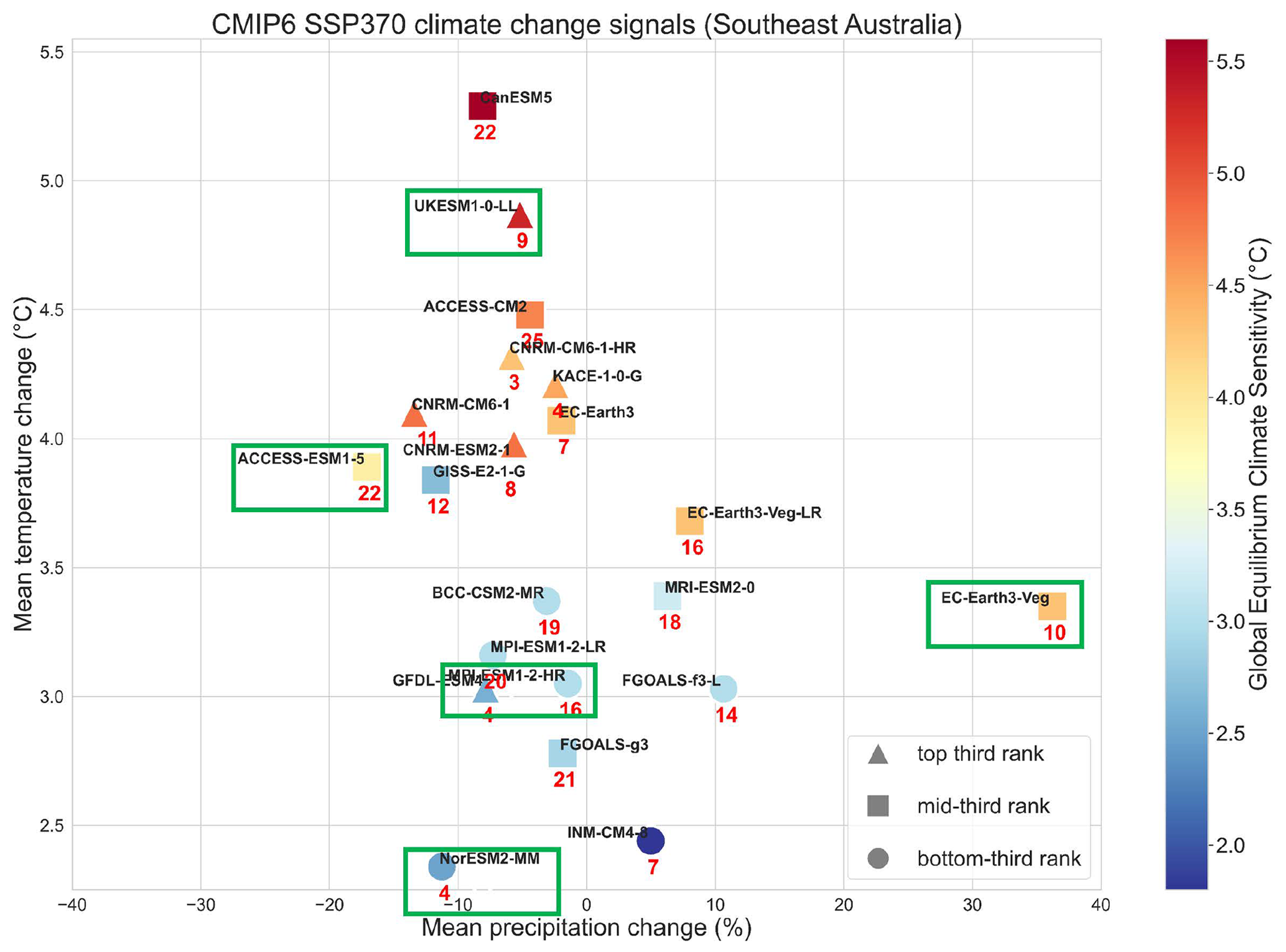
Figure 3 CMIP6 GCM climate change signals (2080–2099 versus 1995–2014) over southeast Australia for the subset of GCMs retained following the model performance evaluation in Di Virgilio et al. (2022) and that simulated at least monthly mean near-surface air temperature and precipitation for the SSP-3.70 scenario. Boxed GCMs are selected to force NARCliM2.0 RCMs. Marker shapes indicate overall GCM performance; markers are coloured according to their global equilibrium climate sensitivity (ECS) values; red numbers represent the smallest Herger method 1 set for that GCM.

4.3 NARCliM2.0 RCM physics testing

The NARCliM2.0 RCM physics testing aims to identify and exclude RCMs that perform consistently poorly in simulating the southeast Australian climate and to select RCMs that have high statistical independence. The selection of RCMs in NARCliM2.0 involves the creation of a multi-physics ensemble where each RCM uses different physical parameterisations for PBL, microphysics, cumulus, radiation, and LSM. This enables many structurally different RCMs to be constructed and tested. In NARCliM1.0, 36 WRF RCM configurations were designed, tested, and evaluated (Evans et al., 2014). NARCliM2.0 physics testing assesses 78 RCM configurations which are progressively tested via three phases, where each test phase is informed by the outcomes of the preceding phase to systematically remove poor-performing RCM options while facilitating the selection of parameterisations that perform well during testing. The N=36 RCMs tested for NARCliM1.0 were evaluated based on eight representative storm event simulations, with each being 2 weeks in duration (Evans et al., 2014). NARCliM2.0 physics simulations were run over an entire annual cycle (2016) with a 2-month spin-up period commencing on 1 November 2015. Australia experienced a range of weather extremes during 2016 driven by a range of climatic influences, making 2016 a suitable target year (Bureau of Meteorology, 2017). Whilst assessing RCMs for an entire year improves on assessing for discrete storm events as per physics testing for NARCliM1.0, it was not feasible to run a large RCM physics ensemble for a longer duration. Initial and boundary conditions for all phases of the NARCliM2.0 RCM physics test simulations were derived from the ERA-Interim reanalysis dataset (Dee et al., 2011). ERA-Interim was used because ERA5 was not available at the time. The three phases of NARCliM2.0 physics testing are as follows.

4.3.1 Phase I (N=36)

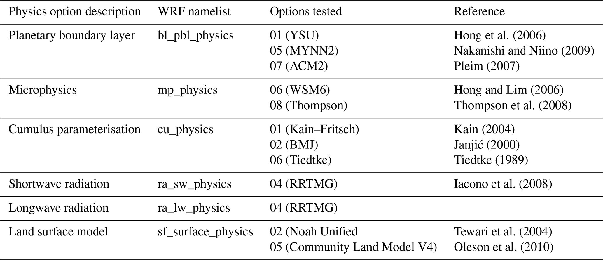
In total, 36 RCMs were evaluated in phase I. One radiation scheme (RRTMG) was tested for both long- and shortwave radiation (it was held fixed for all RCMs), whereas physics settings for PBL, microphysics, cumulus, and LSM were varied. Of the 36 simulations, 18 used the Noah Unified LSM, whilst the remainder used Community Land Model version 4.0 (CLM4). The physics options tested are listed in Table 3, where these were selected based on literature review. Each physics test simulation is denoted by a 12-digit identifier which comprises six pairs of digits, with each pair corresponding to the choice of a specific physics option as specified in the WRF namelist.input file. These pairs of digits follow the order: planetary boundary layer (pbl) | cloud microphysics (mp) | cumulus convection (cu) | shortwave radiation (sw) | longwave radiation (lw) | LSM (sf) and correspond to the WRF namelist options shown in Table 3. For example, simulation 050601040402 is interpreted as 05 | 06 | 01 | 04 | 04 | 02 and denotes that this simulation uses the following physics settings:

bl_pbl_physics	=05 (MYNN2),
mp_physics	=06 (WSM6),
cu_physics	=01 (Kain–Fritsch),
ra_sw_physics	=04 (RRTMG),
ra_lw_physics	=04 (RRTMG),
sf_surface_physics	=02 (Noah Unified).

The complete set of WRF RCM configurations tested in phase I is shown in Table S2 in the Supplement.

Table 3 Physics options used in phase I (N=36) tests.

4.3.2 Phase II (N=60): additional LSM and radiation scheme tests

Phase I RCMs using CLM4.0 were omitted from further testing because they did not consistently improve performance in simulating the Australian climate relative to RCMs using Noah Unified. In addition, RCMs using CLM4.0 had increased simulation times (by approximately twice when compared to Noah Unified). Hence, phase II focused exclusively on further testing of the RCM configurations that used the Noah Unified LSM.

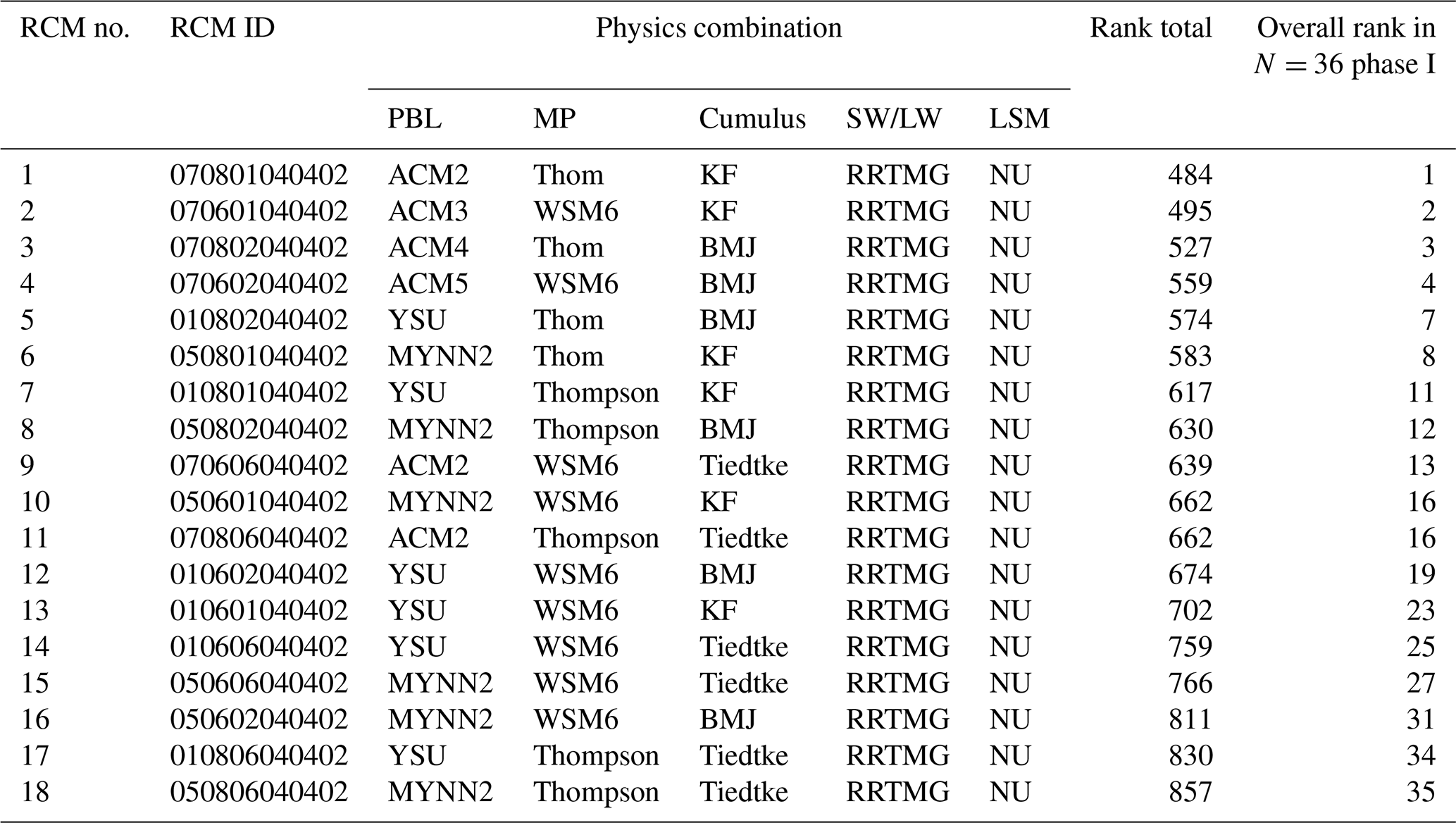
The physics settings tested in phase II are an alternative LSM to Noah Unified (Noah multi-parameterisation, Noah-MP; Niu et al., 2011) and New Goddard (NG) radiation (Chou et al., 2001). Owing to time and resource constraints, testing all 18 phase I RCMs using Noah Unified was not feasible. To reduce the number of RCMs for further testing, the worst-performing Noah Unified-based RCM configurations identified in phase I were excluded. The N=18 RCMs using Noah Unified are listed along with their overall performance total scores in Table 4, where the lowest scores under “Rank total” indicate the RCMs that overall perform relatively well versus their peers (see Sect. 3, “Evaluation methods”). Note that the overall rank denotes the RCMs' relative ranking among all phase I RCMs. There is a sharp reduction in rank totals for RCMs no. 13–18 inclusive relative to RCMs no. 1–12. Therefore, RCMs no. 13–18 are excluded from further testing, and RCMs no. 1–12 are retained.

Table 4 RCM physics combination ranks of the phase I, N=18, Noah Unified-based (NU-based) RCMs. Scores/ranks are based on model bias and root mean square error for annual and seasonal precipitation, minimum temperature, maximum temperature, climate extremes (wettest and hottest days), and Perkins' skill scores (see Sect. 3). RCMs no. 1–12 are selected for further testing.

This gives two sets of physics combinations for additional testing: (1) one replaces only RRTMG (04|04) for short- and longwave radiation with New Goddard (05|05), making no other changes, and (2) RRTMG radiation is retained, but Noah-MP (04) replaces Noah Unified (02). This creates an additional 24 RCM configurations for assessment, bringing the total number of RCMs tested to 60. Although Noah-MP has several parameter options, phase II uses its default settings.

4.3.3 Phase III (N=78): parameterising Noah-MP

Phase II shows that RCM performance using New Goddard radiation is generally inferior to the same RCMs using RRTMG (see Sect. 5, “RCM physics test results”). Consequently, RRTMG radiation is re-adopted for phase III. Conversely, a general performance improvement is conferred using Noah-MP over Noah Unified (Sect. 5). Given this performance improvement using Noah-MP with default settings, phase III assesses RCM performances using specific parameter settings for Noah-MP.

Noah-MP provides a dynamic vegetation cover model option (referred to as dynamic vegetation in the WRF users' guide) (Niu et al., 2011). When deactivated (the default), the monthly leaf area index (LAI) is prescribed for various vegetation types, and the greenness vegetation fraction (GVF) comes from monthly GVF climatological values. Conversely, when dynamic vegetation cover is activated, LAI and GVF are calculated using a dynamic leaf model. We clarify here that dominant plant functional types do not change when using this option but only the LAI and GVF, i.e. only the intensity of green cover changes.

Noah-MP also provides several options for modelling surface runoff and groundwater processes, including a TOPMODEL (TOPography based hydrological MODEL)-based surface runoff scheme and a simple groundwater model (SIMGM; Niu et al., 2011). Some studies have shown that using this option improves the modelling of soil moisture (e.g. Zhuo et al., 2019). Thus, three new sets of physics configurations are tested using Noah-MP, where the default options for specific settings are changed as follows:

1. Activate dynamic vegetation cover (dveg = 2 in the WRF namelist); no other changes.

2. Activate TOPMODEL runoff with simple groundwater (opt_run = 1); no other changes.

3. Activate both dynamic vegetation and TOPMODEL runoff with simple groundwater; no other changes.

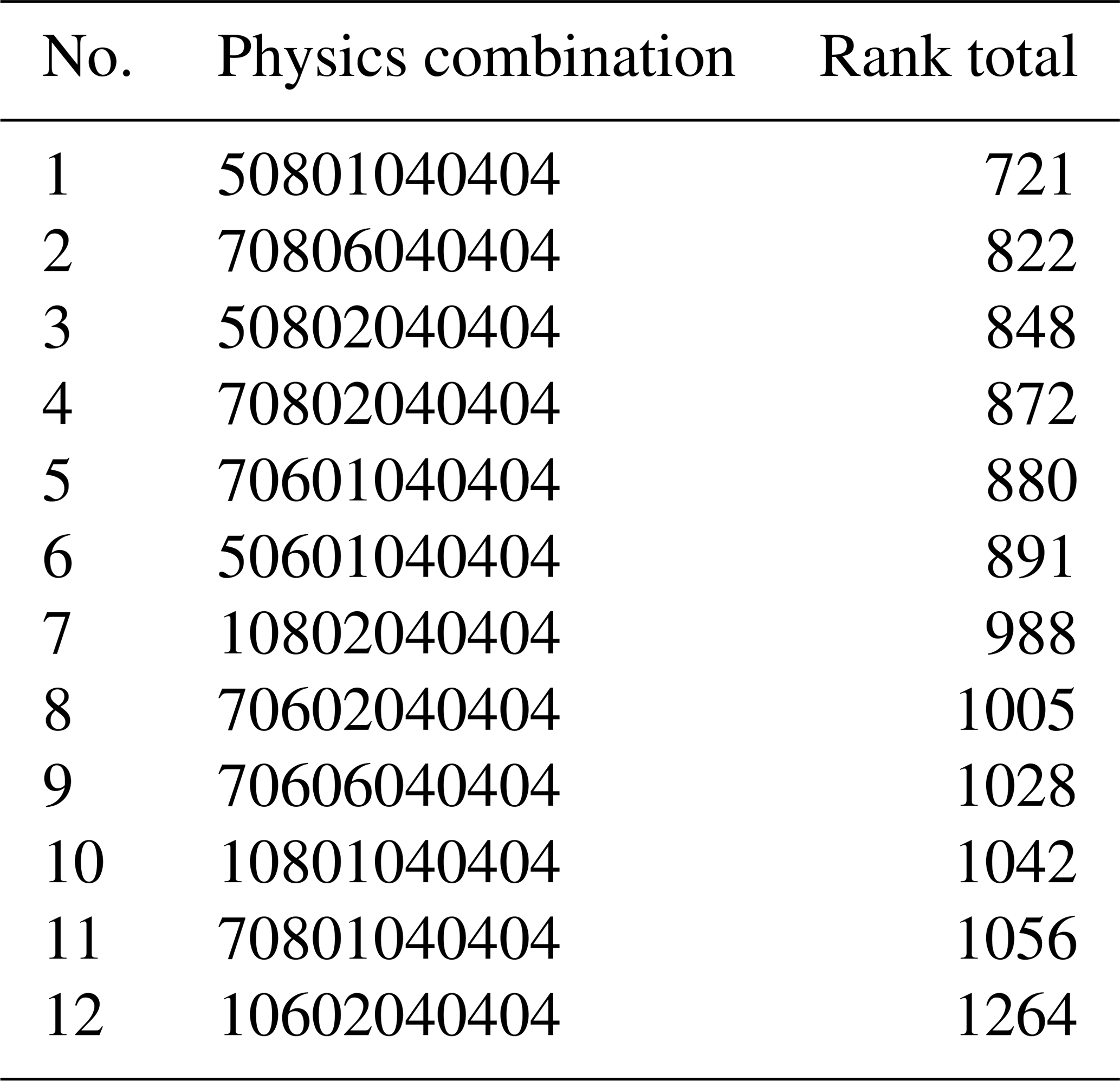
As above, the worst performing RCMs in phase II are excluded from phase III testing. Based on the RCM configuration performance rankings (Table 5), there is a sharp reduction in performance starting from RCM no. 7 inclusive. Therefore, RCMs no. 7–12 are excluded from further testing. Phase III thus comprises 18 new test simulations (sets 1–3, each comprising six RCMs), bringing the total RCMs tested to N=78. Phase III physics tests are denoted using the same RCM identification schemes distinguished by appending set_1, set_2, and set_3 to identifiers.

Table 5 RCM physics combination ranks of the phase II Noah-MP RCMs. Scores/ranks are based on model bias and root mean square error for annual and seasonal precipitation, minimum temperature, maximum temperature, climate extremes (wettest and hottest days), and Perkins' skill scores (see Sect. 3).

4.3.4 Shortlisting physics test RCMs for ERA5-NARCliM2.0 evaluation simulations

Considering the complete NARCliM2.0 N=78 physics test ensemble, to identify physics test RCMs that perform poorly overall, RCMs are eliminated if they are in the lowest one-third for RCM performance ranks for any of maximum temperature, minimum temperature, or precipitation or for the overall model performance rank across these variables (see Sect. 5, “RCM physics test results”). Using this scheme, 20 RCMs remain. The independence measures are then applied to the remaining 20 RCMs to choose a final subset of seven RCMs for ERA5-forced evaluation simulations (see Sect. 4.4). The ensemble size limit of N=7 is determined by available computing resources. These seven candidate RCMs are assessed for potential use in the CMIP6 GCM-forced downscaling phase of NARCliM2.0 (Sect. 4.4 and Di Virgilio et al., 2025).

4.4 CORDEX ERA5-NARCliM2.0 evaluation simulations

NARCliM1.x performed production climate simulations using a two-phase process. Its RCM physics testing selected definitive production-grade RCMs which were then used to downscale both reanalysis data and CMIP3/5 GCMs. In contrast, for NARCliM2.0 as described above the N=78 RCM, physics testing culminates in shortlisting seven production-candidate RCMs, which are used to downscale the ERA5 reanalysis for 42 years (1979–2020). This enables the assessment of the performances of these seven shortlisted RCMs over a climatological period rather than the single year (2016) of the physics testing, which helps ascertain that performance differences between shortlisted RCMs are robust across a multidecadal timescale, capturing climatologically diverse years. The aim is that two definitive production-grade RCMs can be selected for CMIP6-forced downscaling from these ERA5-forced CORDEX evaluation simulations. Thus, the seven ERA5-NARCliM2.0 RCMs were driven by ERA5.0 boundary conditions for January 1979 to December 2020 using the model and nested domain setups described above for NARCliM2.0. The skill of these RCMs in simulating the recent Australian climate was assessed as follows (see Di Virgilio et al., 2025): annual and seasonal means were calculated for maximum and minimum temperature and precipitation using monthly means for temperature variables and the monthly sum for precipitation. Extremes of maximum temperature and precipitation (99th percentiles) and extreme minimum temperature (1st percentile) were calculated using daily data. RCM performances in reproducing observations at these timescales were assessed by calculating model outputs without observations (i.e. model bias) and the RMSE of modelled versus observed fields. The RCM skill in simulating distributions of observed variables was assessed by comparing the PDFs for daily mean observations versus those of the RCMs. The ultimate outcome of these ERA5-forced simulations and their evaluation is the selection of two definitive RCM configurations, R3 and R5, to run the CMIP6-forced phase of NARCliM2.0; see Di Virgilio et al. (2025) for further details on the evaluation methods and results. Figure S1 in the Supplement shows the WRF namelist settings for the R3 and R5 RCMs (see also the “Code availability” section).

4.5 CORDEX-CMIP6-forced NARCliM2.0 simulations

The ideal CMIP6 GCM variables and the frequencies required to run the WRF RCM are listed in Table S1. A minority of variables in Table S1 are not available at subdaily frequencies for every target GCM. This necessitates assumptions/data proxies to be made. For instance, soil moisture and soil temperature variables were unavailable for some selected GCMs; hence, surrogate data, such as surface temperature, were used for initialisation (noting that soil data are only used by the RCM at initialisation). In these cases, we investigated how long it took for uncertainty in the initial conditions to disappear from the WRF output by analysing the regionally averaged soil moisture time series. The data were regionalised according to the four Australian natural resource management (NRM) regions/climate zones (Fig. S2 in the Supplement) which are broadly aligned with climatological boundaries (Fiddes et al., 2021) and with the IPCC reference regions (Iturbide et al., 2020). Time series plots (Fig. S3) show that soil moisture equilibrates to be within a normal range following initialisation, indicating that the 12-month spin-up year (1950) is sufficient to account for the assumptions made at model initialisation.

Boundary and initial conditions were prepared using selected GCM data to run the 151-year GCM-driven simulations using WRF version 4.1.2. The GCM-driven simulations were run and completed using the pre-defined RCM settings for the two definitive RCM configurations using the WRF namelists in Fig. S1 in the Supplement (see also the “Code availability” section). A cold restart was performed in the last historical experiment year (2014), thus enabling the SSP1-2.6 and SSP3-7.0 experiments to be run for 2015–2100 concurrently with the historical experiment. Testing the time duration required for soil moisture to equilibrate from the cold start showed that 1 year is sufficient. The 2014 cold-start year is eventually overwritten by historical runs initiated in 1950.

5 RCM physics test results

5.1 Phase I RCM performance summary

The spatial variation and magnitudes for phase I RCM biases and RMSEs for annual mean maximum and minimum temperature and precipitation are shown in Figs. 4 and 5, respectively. Overall, RCMs are biased cold for maximum temperature (mean absolute bias for the ensemble mean = 1.18 K) and warm-biased for minimum temperature (mean absolute bias = 1.31 K; Fig. 4a, b). Maximum temperature RMSE magnitudes are large over the elevated terrain of the southeast coast and over western regions (Fig. 5a). The simulation of precipitation shows biases of varying sign, with wet biases that are strongest over eastern coastal regions (Fig. 4c). Precipitation RMSEs are particularly large along the eastern coastline (>15 mm) and generally show an east–west gradient, i.e. progressively decreasing further inland from the coast (Fig. 5c).

5.2 Comparing phase II physics test RCM performance with that of phase I

5.2.1 Climate means

Overall, the RCM ensemble using New Goddard (NG) radiation has inferior performance to the corresponding RCMs using RRTMG in terms of annual/seasonal mean maximum temperature biases, RMSEs, and PSS (Table 6). In contrast, NG confers superior performance for annual/seasonal mean minimum temperature for these statistics. RCMs using NG show reduced biases for annual mean and spring-time precipitation but larger errors for DJF and JJA (Table 6). RMSEs for annual and seasonal precipitation are similarly variable.

Table 6 Climate means performance: phase II physics tests (i.e. N=12) set 1 changing only RRTMG to New Goddard (NG) and N=12 set 2 changing only land surface model (LSM) from Noah Unified to Noah-MP (NMP) compared with the phase I physics test RCMs that were shortlisted for further testing (N=12). rad.: radiation.

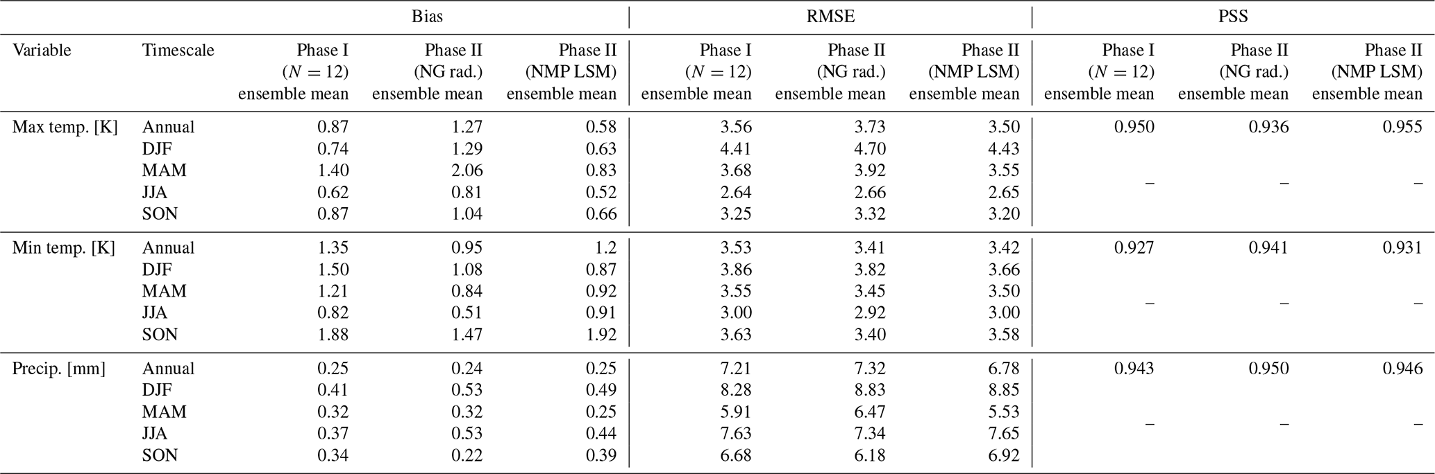
Phase II RCMs using Noah-MP with RRTMG retained show improved performance in simulating mean maximum and minimum temperatures at annual timescales and most seasons relative to corresponding phase I RCMs using Noah Unified (Table 6; Figs. 4 and 5). For instance, the mean absolute bias for annual mean maximum temperature is 0.58 K for the Noah-MP ensemble mean versus 1.18 K for the Noah Unified ensemble. In particular, cold-bias magnitudes for maximum temperature are considerably lower over eastern and southern regions for the RCMs using Noah-MP (Fig. 4d). RMSE magnitudes for maximum temperature are substantially reduced over the topographically complex regions of the southeast and the southwest and central regions (Fig. 5d).

Overall, the magnitude of warm biases for minimum temperature is broadly similar for phase I and phase II RCMs (Fig. 4b, c). Conversely, while RCMs in both phases show large RMSEs for minimum temperature over several eastern regions, RMSEs are smaller for the Noah-MP ensemble over some southern areas (Fig. 5b, c).

In contrast to the above results for the simulation of maximum temperature, overall, phase II RCMs using Noah-MP show smaller performance improvements for the simulation of precipitation relative to the phase I RCMs (Table 6). However, precipitation bias magnitudes are smaller for the Noah-MP ensemble over specific regions, e.g. northeastern coastal regions and the elevated terrain of the southeast (Fig. 4c, f).

Figure 4 Phase I (N=36), phase II (N=60), and phase III (N=78) ensemble mean biases for annual mean maximum temperature, minimum temperature, and precipitation with respect to Australian Gridded Climate Data (AGCD) observations for NARCliM2.0 phase I physics test RCMs using Noah Unified as the land surface model (LSM) (a–c). Phase II physics test RCMs using Noah-MP as the LSM and its default settings (d–f). Phase III set 1 physics test RCMs using Noah-MP with dynamic vegetation cover activated (g–i). Phase III set 2 physics test RCMs using Noah-MP with TOPMODEL surface runoff and simple groundwater activated (j–l). Phase III set 3 physics test RCMs using Noah-MP with both dynamic vegetation cover and TOPMODEL runoff activated (m–o).

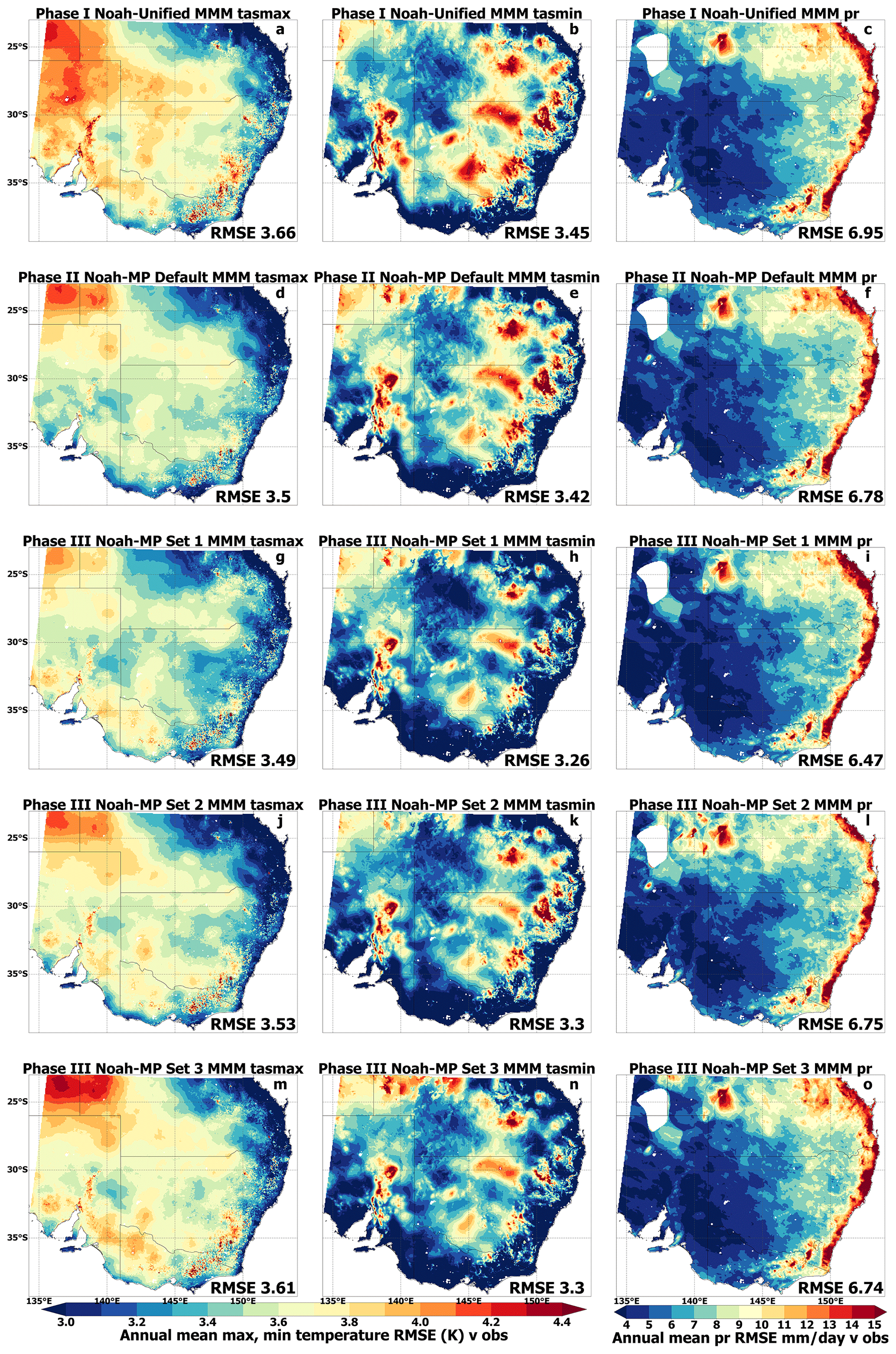
Figure 5 As in Fig. 4 but showing RMSEs.

5.2.2 Climate extremes

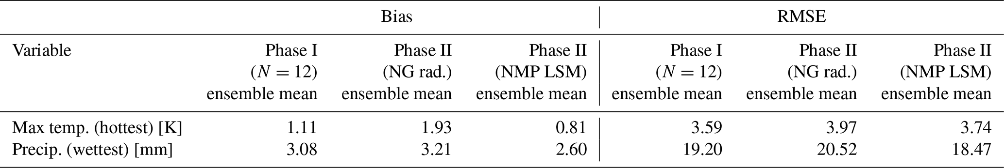
Climate extreme analysis assesses RCM representations of the hottest and the wettest day versus AGCD. For both extremes and for RCM biases and RMSEs, phase II RCMs using NG radiation showed inferior performance relative to phase I RCMs using RRTMG (Table 7). Conversely, phase II RCMs using Noah-MP show substantial reductions in bias for both the hottest and the wettest days (Table 7). Phase II Noah-MP RCMs show a small increase in RMSE for the hottest day (phase I bias = 3.59 K; phase II bias = 3.74 K); however, RMSEs are smaller for the wettest day (i.e. phase I RMSE = 19.20 mm; phase II RMSE = 18.47 mm) (Table 7).

Table 7 Climate extremes performance – comparing phase I RCMs (N=12) with phase II RCMs (i.e. 12 RCMs changing radiation (rad.) from RRTMG to New Goddard, NG, and 12 RCMs changing land surface model (LSM) from Noah Unified to Noah-MP, NMP).

5.3 Phase III RCM performance summary and shortlisting N=7 RCMs for ERA5-NARCliM2.0 evaluation simulations

Overall, RCM biases for mean maximum temperature do not show marked improvements once the dynamic vegetation cover and surface runoff options are activated for Noah-MP (Fig. 4g, j, m) relative to RCMs using Noah-MP with default settings (Fig. 4d). However, specifically for the RCM ensemble with dynamic vegetation cover activated for Noah-MP, RMSE magnitudes for maximum temperature are lower over some eastern coastal regions (Fig. 5g).

The simulation of mean minimum temperature shows clear performance improvements for phase III RCMs using options activated for Noah-MP, relative to RCMs using Noah-MP defaults. Overall, both biases and RMSEs for minimum temperature are reduced in magnitude for RCMs using either of dynamic vegetation cover and runoff/groundwater options activated for Noah-MP or both relative to the default parameters (Figs. 4 and 5). These performance improvements are the largest over eastern and southern regions.

There are no substantial overall performance improvements in the simulation of precipitation for phase III RCMs relative to phase II RCMs (Figs. 4 and 5f, i, l, o). However, using Noah-MP with specific LSM options remains favourable to using RCMs with Noah Unified although the performance gains are generally small, except for some coastal regions and especially the northeast.

All 78 RCMs in the complete RCM physics test ensemble are ranked for performance as described in Sect. 3.2. Once the poor-performing RCMs are excluded, there are 20 RCMs remaining (Table 8; Figs. 6–8). In Table 8, we see that 16 Noah-MP-based RCMs from phase II and phase III comprise this set of 20 RCMs, with 3 of the 20 RCMs using Noah Unified and 1 using CLM4.0. For maximum temperature, some shortlisted RCMs show substantial RMSEs over northwestern and inland areas (e.g. Fig. 6d–f) that are of a larger magnitude over these areas than the ensemble means of phase I-III RCMs (Fig. 5). Conversely, several shortlisted RCMs show very low RMSEs for maximum temperature across eastern and southern regions, especially along the eastern coast (Fig. 6, e.g. RCMs in panels d, l, n, o, q). For minimum temperature, a subset of the 20 shortlisted RCMs show substantially reduced RMSEs over many regions relative to the Phase I–III ensemble means (Fig. 7, e.g. RCMs in panels b, h, i). Additionally, several shortlisted RCMs show reduced RMSEs for precipitation over the eastern coast and northeast (Fig. 8, e.g. RCMs in panels c, l, m, n, o) relative to the Phase I–III RCM ensemble means in Fig. 5c, f, i, l, o.

These 20 RCMs are assessed for statistical independence and seven RCMs from this RCM set are shortlisted for the ERA5-forced RCM simulations considering both their performance and independence scores (Table 8). These seven shortlisted RCMs are listed in bold in Table 8 and are identified as R1–R7 in the ERA5-forced evaluation simulations (Table 8, final column). RCMs are shortlisted from the set of 20 if they rank highly for both performance and independence. For instance, RCM 050801040404_set_3 (Table 8, top row) is top-ranked for performance. However, its independence scores/ranks are low; hence, it is not shortlisted. It is important to note that while a general performance gain is observed in the physics testing when using Noah-MP, there are some specific RCM configurations using Noah Unified that perform well in simulating the Australian climate. For instance, the RCM 010602050502 (R1; Table 8, row 7) uses Noah Unified and performs well overall (its overall performance rank = 7) and especially for the simulation of maximum temperature (Fig. 6a). It is also the only RCM in this set of 20 RCMs to use YSU for PBL. Importantly, this RCM is highly ranked for statistical independence; hence, this RCM is shortlisted for the N=7 set. We note here that R1–R7 is simply a chronological naming convention and does not imply any ranking for these seven RCM configurations.

Table 8 The 20 NARCliM2.0 physics test RCMs shortlisted from the ensemble of 78 RCMs based on their performance in simulating the Australian climate and independence (ind.). N=7 R1–R7 RCMs shortlisted for ERA5-forced evaluation simulations are shown in bold. R1–R7 is a naming convention and does not imply a ranking for these seven RCMs. NU: Noah Unified, NMP: Noah-MP, DV: dynamic vegetation cover, and TOP: TOPMODEL runoff.

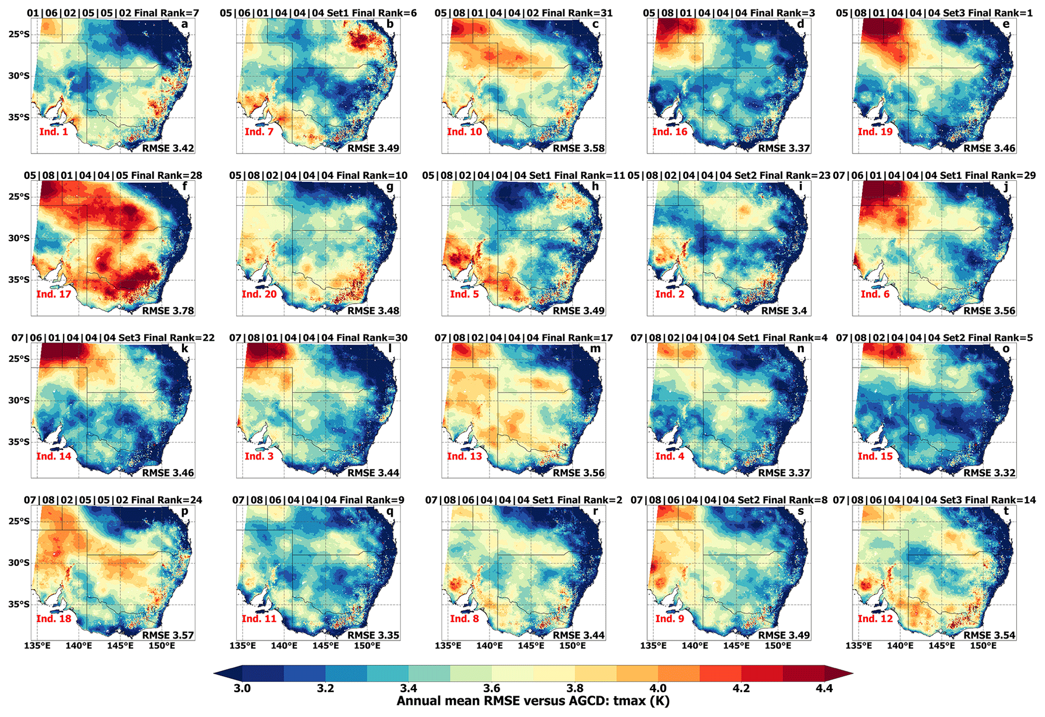
Figure 6 RMSEs for modelled mean maximum temperature (tmax) versus observations for the 20 NARCliM2.0 physics test RCMs shortlisted from the full ensemble of 78 RCMs based on their performance in simulating the recent southeast Australian climate. Overall (final) performance ranks and Bishop and Abramowitz (2013) method independence (ind.) scores are shown.

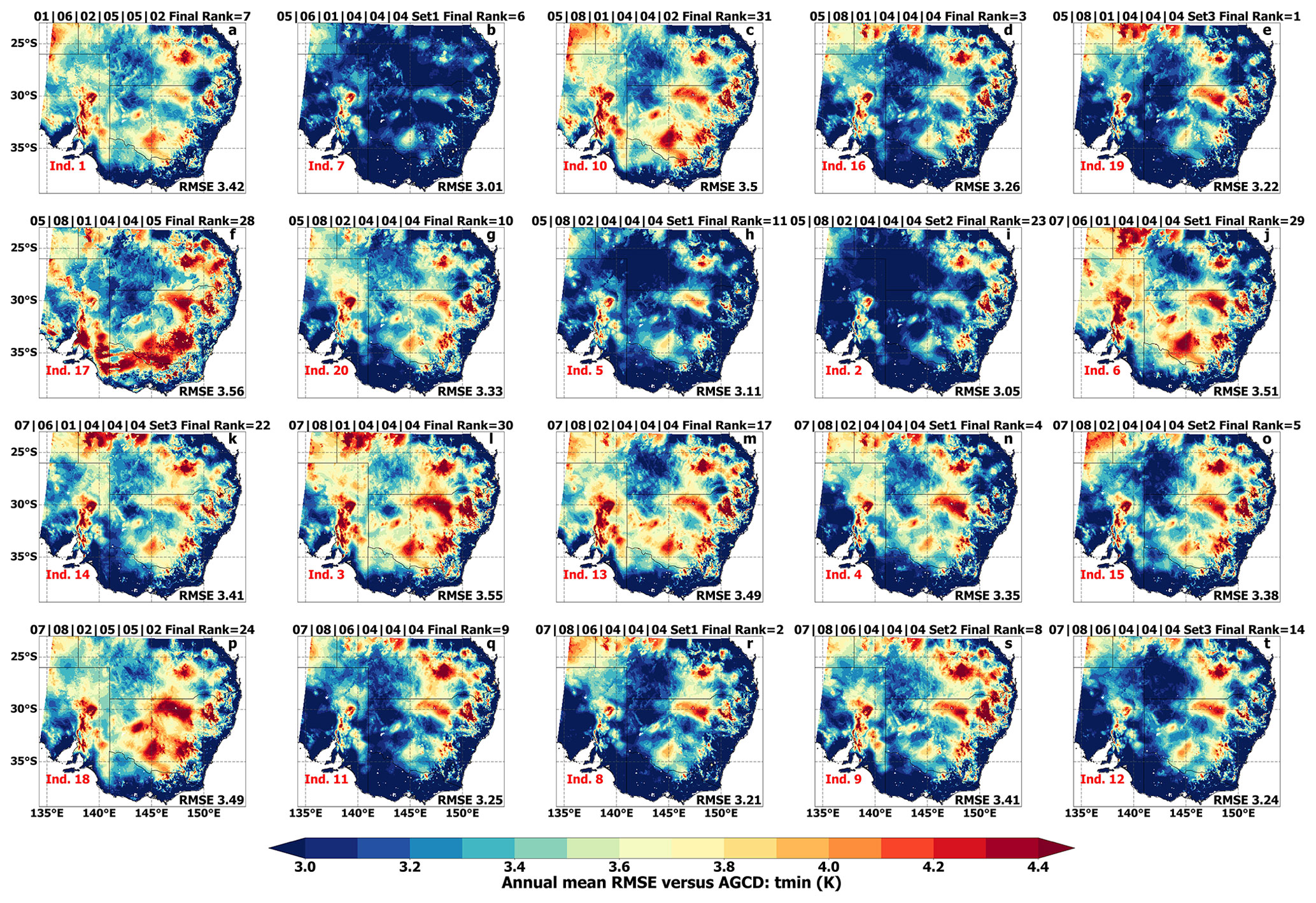
Figure 7 As in Fig. 6 but for mean minimum temperature (tmin).

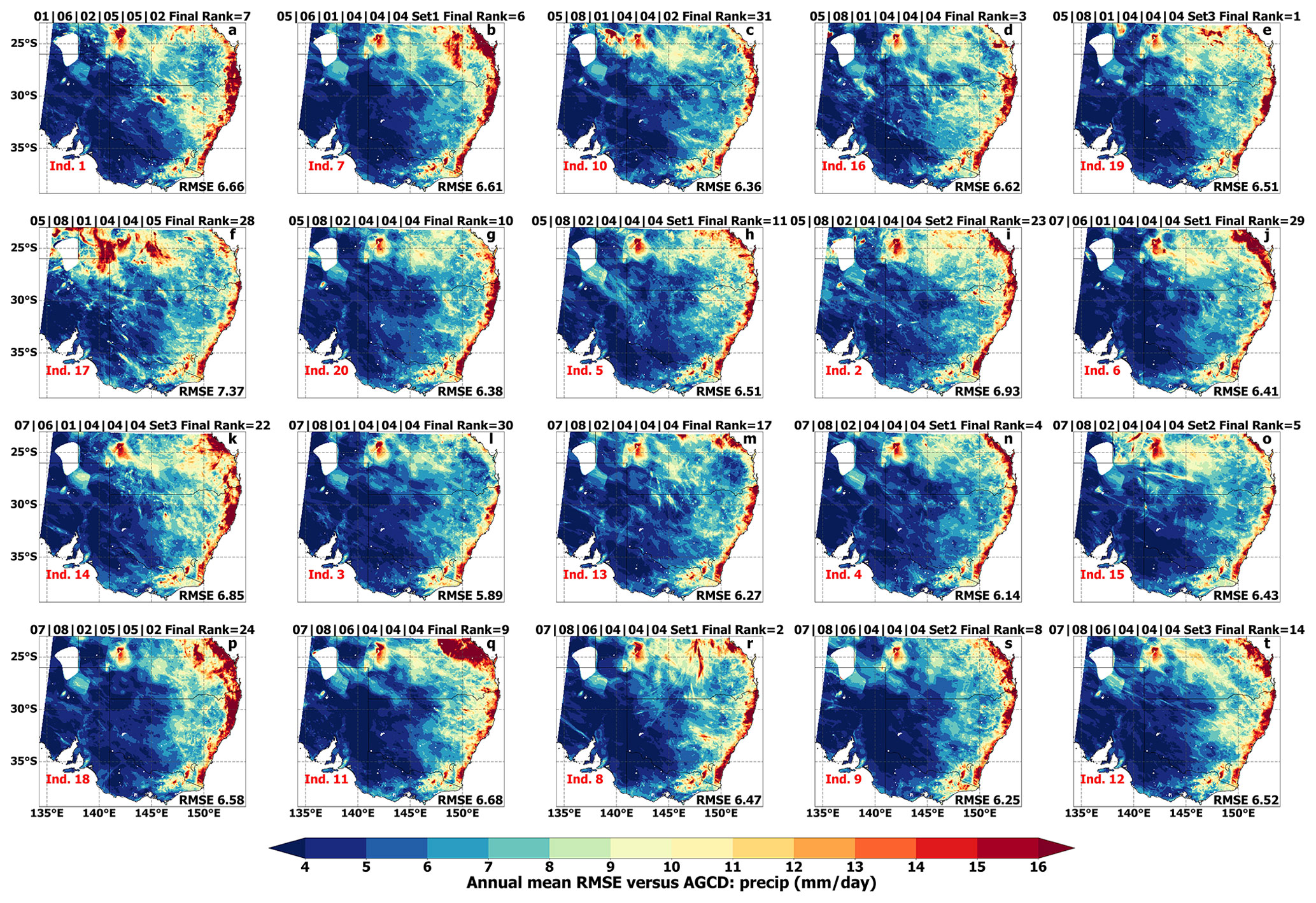
Figure 8 As in Fig. 6 but for mean precipitation (precip).

6 CORDEX-CMIP6 NARCliM2.0 historical evaluation

6.1 Maximum temperature

Overall, NARCliM2.0 RCMs simulate maximum temperature more accurately than NARCliM1.x, with widespread statistically significant reductions in cold biases in the ensemble mean (Fig. 9) as well as for many individual RCMs (Figs. S4–S6 in the Supplement). These reductions in the bias apply to all timescales but are largest for the annual mean, i.e. the area-averaged mean absolute bias for the NARCliM2.0 ensemble is 0.75 K (range from 0.61 to 2.03 K), 1.73 K (range from 1.1 to 2.37 K) for NARCliM1.5, and 1.89 K (range from 0.55 to 4.12 K) for NARCliM1.0 (Fig. 9d, g, j and Fig. S4). Notably, the NARCliM2.0 ensemble mean annual mean maximum temperature bias magnitudes are small, i.e. around <0.5 K, over southwest WA, southern coastal regions, and several eastern regions. This may be important from a climate change adaptation and mitigation perspective as these regions are heavily populated and economically significant. NARCliM2.0 retains warm biases of a similar magnitude to NARCliM1.5 along the northwest coast of Australia (Fig. 9d, g). Moreover, these warm biases cover additional areas for NARCliM2.0, especially during DJF (Fig. 9e, h). A wide range of bias signs is evident for the individual NARCliM2.0 ensemble members (Figs. S4–S6), and a minority of NARCliM2.0 RCMs retain strong cold biases, e.g. at an annual timescale NARCliM2.0-NorESM2-MM R3 (mean absolute bias = 2.03 K) and UKESM-1-0-LL R3 (1.77 K). Additionally, the R5 RCM is generally warmer than R3 (e.g. Fig. S4c, d). Considering the forcing GCM data, overall, ensemble means for the CMIP6 and CMIP5 GCMs generally show similar patterns and magnitudes of cold bias for maximum temperature (Fig. S7 in the Supplement).

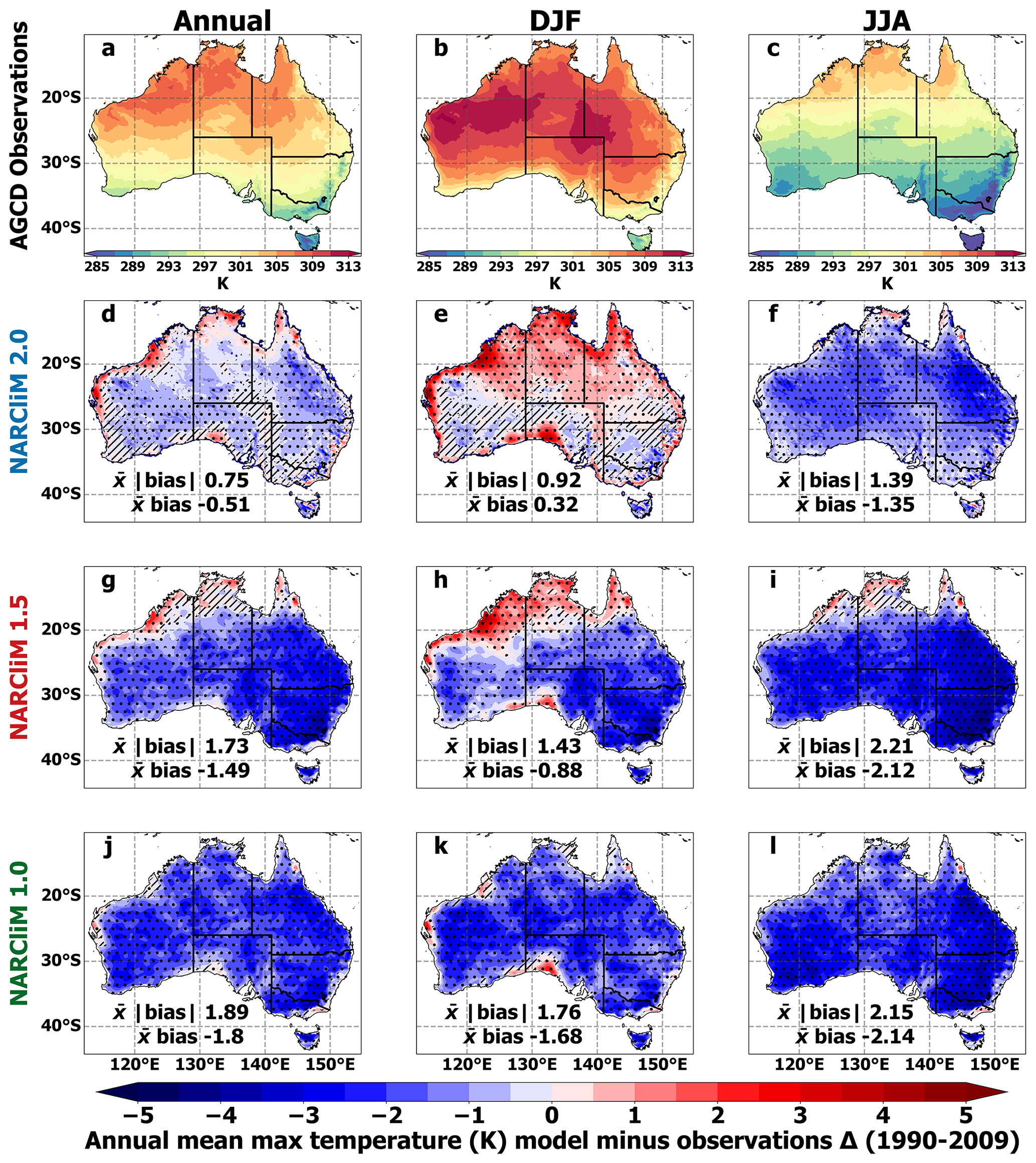
Figure 9 Annual, DJF, and JJA mean near-surface atmospheric maximum temperature biases for NARCliM2.0, 1.5, and 1.0 historical ensemble means with respect to Australian Gridded Climate Data (AGCD) observations for 1990–2009. Stippled areas indicate locations where an RCM shows statistically significant bias. Significance stippling for the ensemble mean bias follows Tebaldi et al. (2011) and is applied separately to each RCM ensemble. Statistically insignificant areas are shown in colour, denoting that less than half of the models are significantly biased. In significant agreeing areas (stippled), at least half of RCMs are significantly biased, and at least 70 % of significant RCMs in each ensemble agree on the direction of the bias. Significant disagreeing areas are shown in hatching, which are where at least half of the models are significantly biased and less than 70 % of significant models in each ensemble agree on the bias direction; see main text for additional details on the stippling regime.

6.2 Minimum temperature

The simulation of mean minimum temperature by NARCliM2.0 is generally warm-biased at all timescales (Fig. 10). Its bias magnitudes over many regions are larger versus NARCliM1.5; e.g. annual mean area-averaged absolute biases are 0.98 and 0.79 K for NARCliM2.0 and NARCliM1.5, respectively (Fig. 10d, g). However, there are exceptions to this result over specific regions; for example, parts of southwest western Australia show annual mean bias magnitudes of <1 K for NARCliM2.0, but these areas show biases below −2 K for NARCliM1.x (Fig. 10d, g, j). Most individual RCMs comprising the NARCliM2.0 ensemble show stronger warm biases than their NARCliM1.5 peers at both annual and seasonal timescales (Figs. S8–S10). The ACCESS-ESM-1-5-forced NARCliM2.0 RCMs are considerably more warm-biased than the other NARCliM2.0 RCMs, with average absolute biases of 1.74 and 1.9 K (Fig. S8c–d).

Many of the CMIP6 GCMs used to force the NARCliM2.0 RCMs are warmer than the CMIP5 GCMs used to force NARCliM1.5 such that the ensemble mean bias of the former is 1.9 K versus 1.11 K (Fig. S11). In particular, ACCESS-ESM-1-5 and MPI-ESM1-2-HR are substantially more warm-biased relative to all other selected GCMs, with mean absolute biases of 2.2 and 3.47 K, respectively (Fig. S11). This suggests that NARCliM2.0's warm biases for mean minimum temperature are at least partially inherited from the driving data. However, whilst the ACCESS-ESM-1-5-forced NARCliM2.0 RCMs are much warmer than their counterparts (i.e. 1.74 and 1.9 K), this does not apply to the MPI-ESM1-2-HR-forced RCMs, which have biases of only 1.01 and 1.09 K. Hence, factors additional to the driving data, such as changes in RCM parameterisations between NARCliM generations and other model design changes likely contribute to the warmer biases observed for NARCliM2.0.

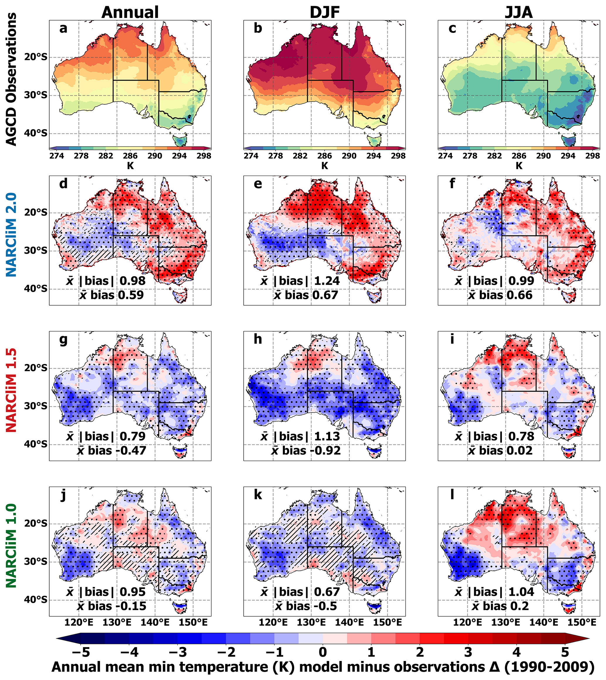
Figure 10 As in Fig. 9 but for mean minimum temperature.

6.3 Precipitation

The NARCliM2.0 ensemble shows small dry biases for mean precipitation over most regions, except for some areas mainly in the east of the country, which show slight wet biases (Fig. 11d–f). This contrasts with stronger wet biases of NARCliM1.5 that are statistically significant over many regions (Fig. 11g–i) and the even stronger wet biases of NARCliM1.0 (Fig. 11j–l). Area-averaged bias magnitudes are considerably smaller for NARCliM2.0 relative to NARCliM1.x, especially for the annual mean, i.e. 8.03 mm versus 16.69 and 33.25 mm, respectively. Annual mean precipitation biases are particularly small over eastern regions, often being <5 mm. NARCliM2.0 retains the strong summertime dry biases for precipitation over northern Australia that are also evident for NARCliM1.5 (Fig. 11e, h), noting that this region also shows strong warm biases for maximum temperature (Fig. 9).

The individual RCMs comprising NARCliM2.0 show a range of results for annual and seasonal mean precipitation biases (Figs. S12–S14). Notably, three of the 10 NARCliM2.0 RCMs have substantially larger bias magnitudes than their peers at annual and summer timescales, i.e. both MPI-ESM1-2-HR-R3 and R5 (absolute biases are 15.53 and 22.45 mm for annual mean precipitation; Fig. S12g–h) and EC-Earth3-Veg-R5 (Fig. S12f; 18.59 mm). Despite EC-Earth3-Veg-R5 being strongly dry-biased, EC-Earth3-Veg-R3 simulates precipitation more accurately; i.e. its mean absolute bias = 9.53 mm (Fig. S12e). Analogously to NARCliM2.0's performance for temperature, R5 is drier than R3. Comparing the ensemble means of the driving GCMs, the CMIP6 GCMs are marginally more accurate in simulating annual mean precipitation than the CMIP5 GCMs (Fig. S15). Whilst the CMIP6 ensemble produces small biases over inland areas, its biases are larger along the east coast.

Figure 11 As in Fig. 9 but for mean precipitation (precip).

7 CORDEX-CMIP6 NARCliM2.0 climate change projections

Dependent on location, the largest maximum temperature projected increases for NARCliM2.0 under SSP3-7.0 are over ∼ 3 K and over ∼ 1.5 K under SSP1-2.6 (Fig. 12a, d). SSP3-7.0-NARCliM2.0 shows faster warming over inland than coastal regions, with greater warming across a horizontal band of the continent during annual and summer timescales (Fig. 12a–b). This contrasts with NARCliM1.5, which shows a north–south warming gradient at annual and seasonal timescales, with its fastest warming rate over northern regions, and NARCliM1.0, which projects the fastest warming over the west (Fig. 12). For NARCliM2.0, the tropical north warms faster during the winter dry season than during the summer wet season under SSP3-7.0, but this is not the case for SSP1-2.6 (Fig. 12b–c; e–f). NARCliM2.0 simulations under SSP3-7.0 show less warming than NARCliM1.5-RCP8.5 but warmer futures than for NARCliM1.0-SRES A2, with differences in the underlying driving GCMs and GHG scenarios likely contributing to these variations in warming. As per NARCliM1.x, all NARCliM2.0 maximum temperature projections significantly agree with all RCMs projecting statistically significant temperature increases.

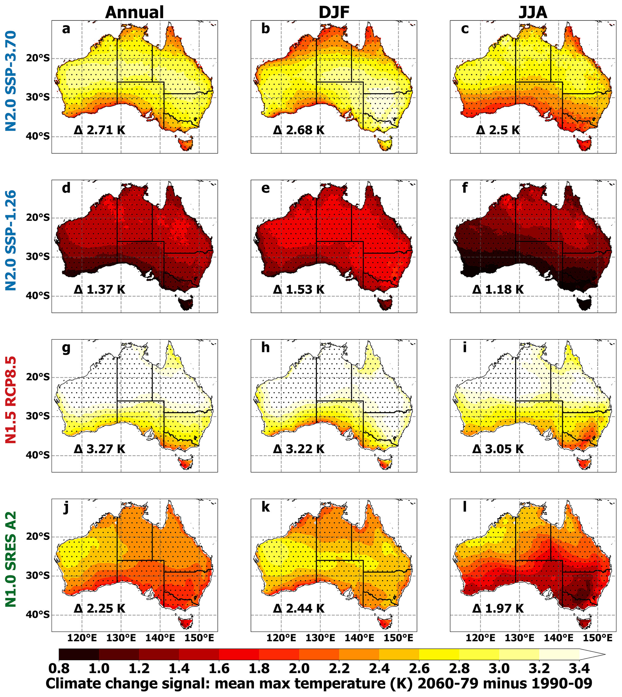
Figure 12 Ensemble mean climate change projections (far future without the present day) for annual, DJF, and JJA mean maximum temperatures, with significance stippling as in Fig. 9.

Projected increases in annual mean minimum temperature for NARCliM2.0 exceed 3 K over some regions for SSP3-7.0 and 1.6 K for SSP1-2.6 (Fig. 13). Under both GHG scenarios, at annual and winter timescales, warming is fastest over northeast Australia. Conversely, NARCliM1.x minimum temperature future increases are generally the largest over northwest or northern Australia, though the summertime projection for NARCliM1.0 is an exception (Fig. 13k). As for maximum temperature projections, all RCMs for all NARCliM generations project statistically significant increases.

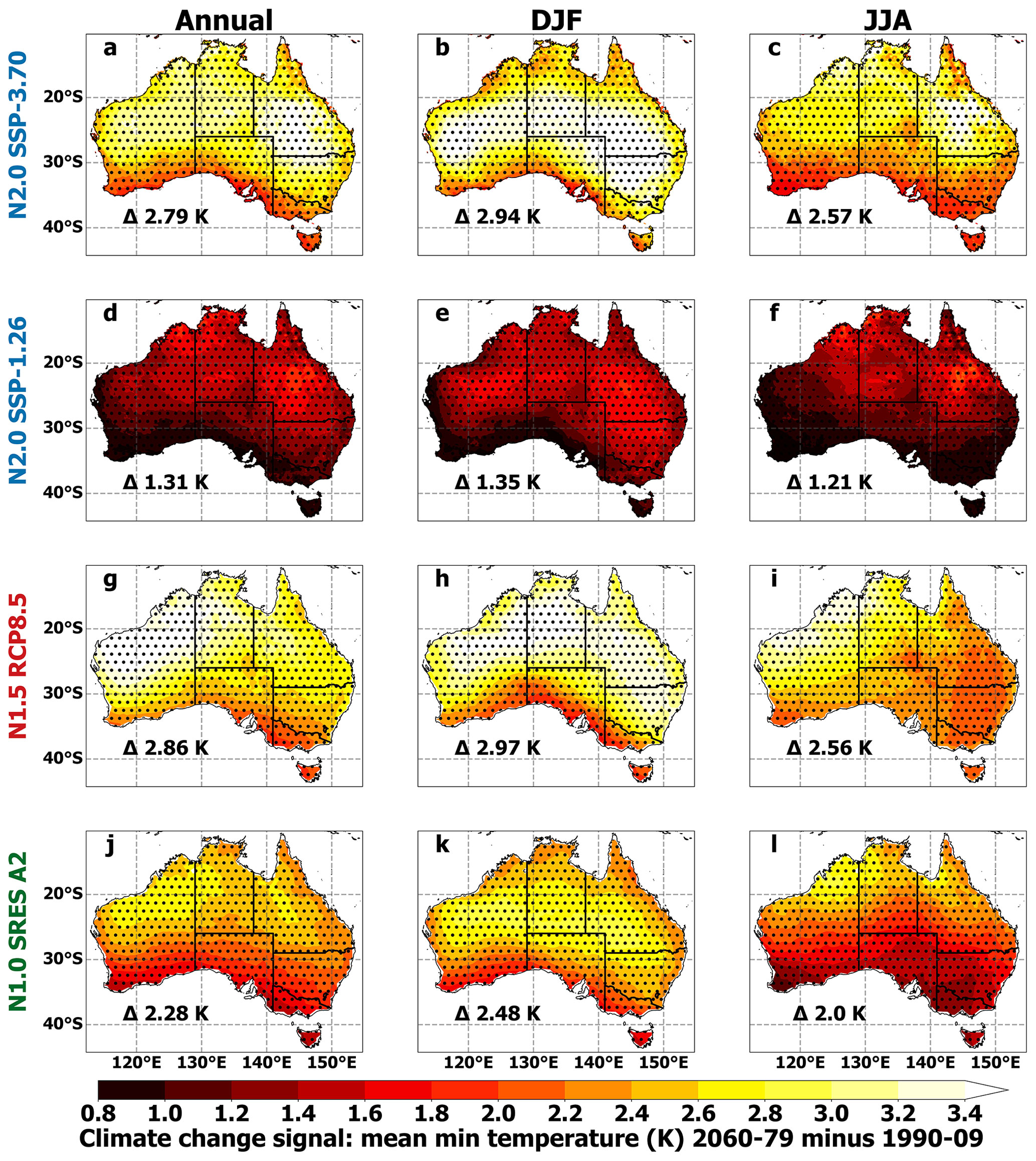
Figure 13 Ensemble mean climate change projections (far future without the present day) for annual, DJF, and JJA mean minimum temperatures, with significance stippling as in Fig. 9.

NARCliM2.0 SSP3-7.0 projects a dry future over most of Australia, except for wetter futures over northern and western regions, which are largest in magnitude in summer (Fig. 14a–b). In contrast, overall, NARCliM2.0 SSP1-2.6 projects dry changes across most of Australia, with the strongest drying over northern Australia during summer (Fig. 14e). Similarities between NARCliM2.0 projections for the low- and high-GHG SSPs include faster drying over the eastern coastline at all timescales, especially during summer. The wetter futures projected by RCMs downscaling SSP3-7.0 GCMs relative to SSP1-2.6 may be partially inherited from the driving CMIP6 GCMs because, overall, SSP3-7.0 GCMs show wetter futures than corresponding SSP1-2.6 GCMs (Fig. S16).

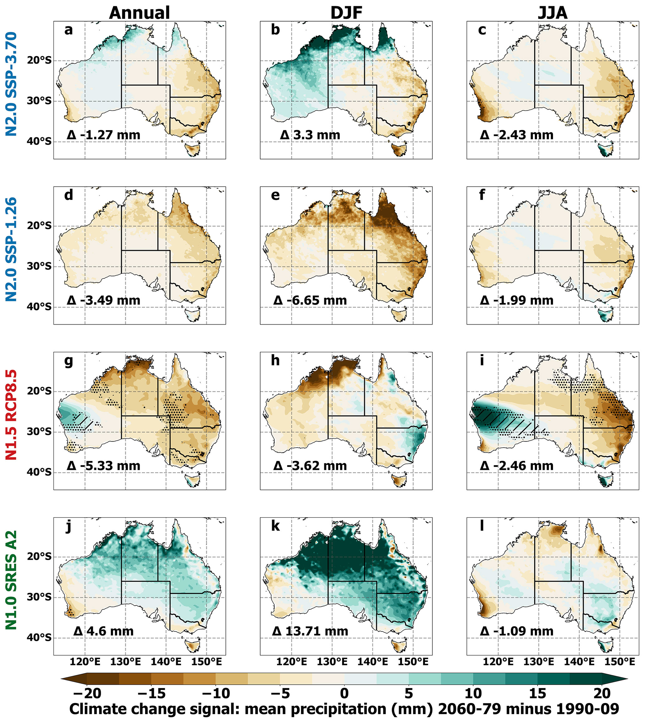
Figure 14 Ensemble mean climate change projections (far future without the present day) for annual, DJF, and JJA mean precipitation, with significance stippling as in Fig. 9.

Considering mean precipitation projections for individual NARCliM2.0 RCMs, in some cases, R3 and R5 RCMs produce similar results when downscaling the same GCM. For instance, ACCESS-ESM-1-5 forced R3 and R5 both show strong projected decreases in annual mean precipitation across Australia (Fig. 15b–c). In contrast, while UK-ESM1-0-LL R3-R5 both show projected decreases in annual mean precipitation over eastern Australia, R3 shows precipitation increases that are substantially more widespread over western and northern regions relative to R5 (Fig. 15j–k). Overall, the NARCliM2.0 ensemble members show a variety of climate change signals for precipitation (Fig. 15) and temperature (not shown), reflecting the range within the larger CMIP6 ensemble (Di Virgilio et al., 2022).

There are some key differences between the mean precipitation projections of NARCliM2.0 relative to those of previous NARCliM generations. For instance, NARCliM1.5 shows stronger reductions in future precipitation over northern and eastern regions at annual and winter timescales (Fig. 14), and these changes are statistically significant over a few regions, whereas projected changes for NARCliM2.0 are largely non-significant. Additionally, NARCliM2.0 projects marked precipitation decreases along the southeast coast during summer, while NARCliM1.5 shows the opposite result (Fig. 14). NARCliM1.0 generally projects wet futures across larger portions of Australia, especially at annual and summer timescales.

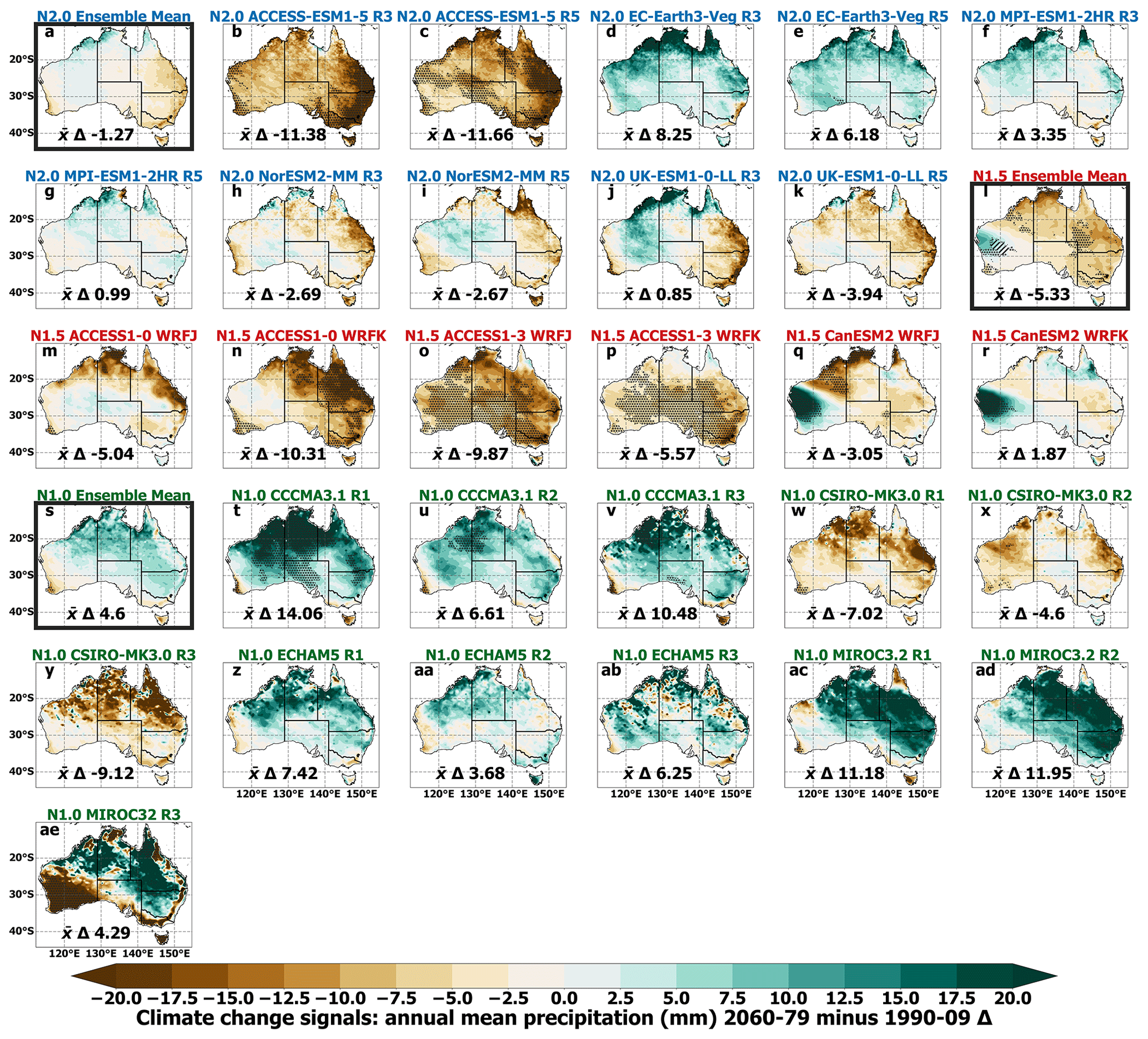
Figure 15 Climate change projections (1990–2009 versus 2060–2079) for annual mean precipitation for NARCliM ensemble mean climate change signals (a, l, s) and for individual ensemble members for each generation of NARCliM simulations (NARCliM2.0 under SSP3-7.0, NARCliM1.5 under RCP8.5, and NARCliM1.0 under SRES A2). Significance stippling as in Fig. 9.

8 Discussion

NARCliM regional climate models produce robust climate projections at spatial scales suitable for local-scale climate change analysis and impact decision-making. The third and latest generation of these regional climate models, NARCliM2.0, encompasses several model design advancements over its predecessors. A key aim of this paper is to describe how NARCliM2.0 differs from its predecessors and explain the rationale behind these design decisions. We also characterise the improvements in model skill in simulating the Australian climate relative to previous NARCliM generations as well as compare climate projections across NARCliM generations. The next section discusses aspects of NARCliM2.0 RCM design and parameterisation in relation to previous studies before reviewing differences in the model biases and the climate projections of the NARCliM2.0 versus NARCliM 1.x RCMs.

8.1 NARCliM2.0 RCM physics testing

In addition to RCM design choices including increased resolution and incorporation of convection-permitting modelling and urban physics, a major change for NARCliM2.0 relative to its predecessors is to use new WRF RCM configurations, which are selected via a large suite of physics tests. RCM performance evaluations for the NARCliM2.0 RCM physics testing focused on the 4 km resolution convection-permitting domain, which does not use a cumulus physics parameterisation. Notably, the seven candidates shortlisted RCMs from the N=78 physics test ensemble used three different cumulus parameterisations for their outer domains, with four RCMs using BMJ, two RCMs using Tiedtke, and one using Kain–Fritsch. This indicates that differences in the outer domain boundary conditions have key influences on the RCM performances in the convection-permitting domain.

Using the Noah-MP LSM in the NARCliM2.0 RCM physics tests conferred overall RCM skill improvements relative to RCMs using the Noah Unified LSM, especially in terms of the simulation of temperature. Although using Noah-MP also improved the simulation of precipitation in some respects, these improvements were smaller relative to the gains for temperature, and improvements were mainly located over coastal regions. The developers of Noah-MP suggest that some limitations in the Noah Unified LSM have been modified to better represent several parameters. These include surface layer radiation balances, snow depth, soil moisture and heat fluxes, leaf area–rainfall interaction, vegetation and canopy temperature distinction, drainage of soil, and runoff.

In the NARCliM2.0 physics testing, improvements in RCM skill were evident for Noah-MP with default settings. Activating specific parameterisations for this LSM (i.e. dynamic vegetation cover and surface runoff–simple groundwater) delivered comparatively smaller gains in RCM performances. Some previous studies have found no overall benefit of using Noah-MP with default settings. For instance, Imran et al. (2018) conducted an evaluation of WRF coupled with a variety of LSMs including Noah-MP using its default settings. They simulated short-duration (∼ 3 d) heatwaves in Melbourne, Australia, and observed larger temperature biases using Noah-MP relative to RCMs using Noah Unified and CLM4.0. However, their focus on specific short-duration heatwave events over one urban area was not intended as a comprehensive evaluation of Noah-MP's performance. Additionally, several physics schemes used by these authors differed from those used in the NARCliM2.0 physics testing; i.e. they used the following: PBL = MYJ; microphysics = Thompson; cumulus = Grell3D; radiation = RRTMG/RRTMG. Only Thompson microphysics and RRTMG radiation are used in the NARCliM2.0 physics testing. WRF and Noah-MP versions also differed; i.e. Imran et al. used WRF3.6.1 and a Noah-MP version prior to 3.7, whereas NARCliM2.0 uses WRF4.1.2 and Noah-MP version 4.1. Additionally, there are also several studies that have reported benefits of using Noah-MP with default parameters relative to other LSMs for other regions globally, such as Chen et al. (2014a, b) and Salamanca et al. (2018).

The NARCliM2.0 physics testing found that the optimal LSM configuration for the simulation of minimum temperature used Noah-MP with dynamic vegetation cover activated, even though the performance gain relative to Noah-MP with default settings was small. Constantinidou et al. (2020) ran WRF coupled with four LSMs (Noah Unified, Noah-MP, CLM, and Rapid Update Cycle) over the Middle East North Africa CORDEX domain. They compared the performance of Noah-MP with dynamic vegetation cover turned on and off and found that air and land temperatures were best simulated using Noah-MP with dynamic vegetation cover activated.

In terms of other NARCliM2.0 RCM parameterisations, focusing on PBL, by the completion of phase I physics testing, only 3 out of 12 RCMs shortlisted for further testing use the YSU scheme. By the completion of phase II testing, all remaining RCMs using YSU are discarded, with only RCMs using PBL schemes other than YSU remaining (i.e. ACM2 and MYNN2). YSU PBL is a first-order closure scheme that expresses turbulent mixing via mean variables rather than prognostic variables (Hong et al., 2006). It is classed as a non-local scheme because it estimates turbulent mixing by small-scale eddies as well as representing transport caused by convective large eddies. Two previous studies evaluating convection-permitting WRF simulations using different parameterisations that included YSU for the PBL scheme found that, relative to other PBL schemes, YSU produced the highest bias for simulated precipitation (Huang et al., 2023; Nuryanto et al., 2019). However, these studies focused on different regions globally and used various experimental setups that are not directly comparable to those used here. Hence, a separate study investigating sensitivities of the NARCliM2.0 RCMs to the different PBL schemes is currently underway.

8.2 CORDEX-CMIP6 NARCliM2.0 historical evaluation

We characterised the improvements conferred by NARCliM2.0 over its predecessors in simulating the present-day Australian climate. NARCliM2.0 simulates mean maximum temperature and precipitation more accurately than NARCliM1.x. Specifically, NARCliM1.x has strong maximum temperature cold biases which are in keeping with other downscaling projects of the CMIP3-CMIP5 eras (e.g. Andrys et al., 2016 and J. P. Evans et al., 2020), but these are substantially reduced in NARCliM2.0. A contributing cause of CMIP5-forced RCM cold biases of maximum temperature is their overestimation of precipitation (J. P. Evans et al., 2020). This relationship was also noted in ERA-Interim-forced RCMs of this same modelling era (Di Virgilio et al., 2019). In NARCliM2.0, the widespread wet biases that characterise the NARCliM1.x RCMs are reduced in magnitude. NARCliM2.0 produces smaller wet biases over eastern Australia and smaller dry biases elsewhere, except for in Australia's tropical north. This marked reduction in wet bias magnitudes is one plausible contributing factor for the reduction in maximum temperature cold bias for the NARCliM2.0 RCMs. The CMIP6 and CMIP5 GCMs used to drive NARCliM2.0 and 1.5 RCMs generally show similar magnitudes of maximum temperature cold bias. This suggests that the underlying nature of the CMIP6 driving data is not a principal factor underlying the observed improvements for NARCliM2.0's simulation of maximum temperature. In fact, the RCMs appear to have a substantial influence on the reduced maximum temperature biases.

The fact that NARCliM2.0 underestimates precipitation over tropical northern Australia during the wet season (summer) to a similar degree of magnitude to the NARCliM1.5 RCMs indicates that the newer models still struggle to accurately capture the strength of the Australian monsoon. The fact that NARCliM1.x strongly overestimates precipitation over southeastern Australia, whereas wet biases over this region are reduced for NARCliM2.0, indicates that the newer models may confer an improved simulation of broad-scale processes associated with synoptic-scale systems interacting with the extratropical storm track over Australia (Grose et al., 2019).

The extent to which NARCliM2.0's improved simulation of precipitation might be attributable to its driving data warrants consideration. Overall, the CMIP6 GCMs used to drive NARCliM2.0 show marginally reduced wet biases versus the CMIP5 GCMs used for NARCliM1.5 (e.g. area-averaged ensemble mean absolute biases are 7.13 and 8.89 mm, respectively; Fig. S15 in the Supplement). This suggests that the underlying nature of the CMIP6 driving data might not be the principal factor underlying the observed improvements for NARCliM2.0's simulation of mean precipitation. Conversely, in terms of RCM design features, the use of the Noah-MP LSM in the NARCliM2.0 RCM physics tests conferred overall RCM skill improvements relative to RCMs using the Noah Unified LSM for both mean precipitation and mean maximum temperature. As noted above, the developers of Noah-MP suggest that some features of the Noah Unified LSM have been modified to better represent several parameters. The production NARCliM2.0 RCMs used Noah-MP, whereas NARCliM1.x RCMs used Noah Unified. Given these performance improvements observed for RCMs using Noah-MP versus using Noah Unified, it is plausible that the newer LSM contributes to the improved NARCliM2.0 skill in simulating precipitation and maximum temperature, for instance, via changing the land surface feedback (via soil moisture) to the simulation of precipitation. This possibility requires more extensive investigation via future studies.

More generally, the scope of the present study was to focus on an initial first-order evaluation of mean precipitation rather than extremes of precipitation. However, clearly valuable research into evaluating the skill of NARCliM2.0 in simulating extreme precipitation, subdaily precipitation, etc. can now be undertaken using NARCliM2.0 20 and 4 km data, and we note that these data are now publicly available. A good avenue for further research is to assess the potential added value in simulating extreme and subdaily precipitation at a convection-permitting scale versus the convection-parameterised 20 km data. Several previous studies have confirmed that convection-permitting resolution models can improve the simulation of daily and subdaily rainfall extremes (Xie et al., 2024; Cannon and Innocenti, 2019; Kendon et al., 2017).

NARCliM2.0 RCMs overestimate minimum temperatures across Australia, and these biases are larger relative to NARCliM1.5 but comparable to those of NARCliM1.0. The CMIP6 GCMs used to force NARCliM2.0 show substantially stronger warm biases for minimum temperature than the CMIP5 GCMs used for NARCliM1.5. This suggests that the increased warm bias for minimum temperature in NARCliM2.0 RCMs could be partially inherited from the driving GCMs. However, Noah-MP's simulation of factors such as LAI and other aspects of vegetation as well as surface albedo in semi-arid and arid areas has been shown to have deficiencies (Glotfelty et al., 2021). These issues may contribute to some of the biases shown by the NARCliM2.0 RCMs. Moreover, the NARCliM2.0 ensemble mean reduces the overall minimum temperature bias of the CMIP6 GCM ensemble by almost half, attesting to the added value conferred by the NARCliM2.0 RCMs with respect to near-surface temperature variables.

Consideration of observational uncertainty is warranted. We have evaluated NARCliM RCM skill via comparison with AGCD observations. Whilst AGCD is a high-quality gridded observational dataset, like any set of observations, it contains errors and uncertainties. Consequently, the outcomes of our evaluations depend on both models being evaluated and the AGCD observational dataset. This is clearly a broader issue that applies to any model evaluation versus observations. Uncertainties in AGCD for temperature and precipitation arise from sparse station coverage in some locations, especially in remote areas, and interpolation errors in generating gridded data. More specifically, temperature uncertainties include urban heat island effects, inhomogeneities in observation records, and elevation differences. Precipitation uncertainties involve underestimation of extremes, rain gauge measurement errors, and challenges in representing complex terrain. For our purposes, the question of how much of the model bias of ∼ 0.5 K is due to the model errors versus the observational uncertainty cannot be currently quantified because the models are evaluated against this single observational dataset. This leaves the observational uncertainty as implicitly included in our results. In the future observational uncertainty could be explicitly considered using a method like the observation range adjusted (ORA) statistics (Evans and Imran, 2024).

8.3 CORDEX-CMIP6 NARCliM2.0 climate change projections

In terms of NARCliM2.0 future climate projections, major changes between NARCliM generations such as differences in GHG scenarios mean that NARCliM2.0 projected temperature changes differ in some respects to those of its predecessors. Overall, as is expected, projected warming is less intense in NARCliM2.0 under SSP3-7.0 than for NARCliM1.5 under RCP8.5. Other differences in the projections between NARCliM generations require further investigation in order to be explained, such as NARCliM1.5's latitudinal warming gradient for maximum temperature that contrasts with NARCliM2.0's band of faster warming over central Australia relative to northern and southern regions. Irrespective of these differences, all three NARCliM ensembles show widespread statistically significantly agreeing results for warming projections.

Precipitation projections for the different NARCliM generations show some key similarities, such as reductions in mean annual precipitation over eastern Australia for NARCliM2.0 and NARCliM1.5, though a difference is that these are statistically significant over some areas only for NARCliM1.5. NARCliM2.0-SSP3-7.0 and SSP1-2.6 ensembles differ in that the former generally projects wet changes over northern and western Australia, whereas the latter is generally dry, the results that appear being partially traceable to the underlying driving CMIP6-SSP data (Fig. S16 in the Supplement).

Some NARCliM2.0 RCMs produce very similar precipitation projections for certain GCM–RCM combinations. Notably, ACCESS-ESM-1-5-R3 and R5 under SSP3-7.0 both produce widespread dry projections that are substantially drier than other NARCliM2.0 models. This GCM projects very dry futures across Australia (Di Virgilio et al., 2022), so this result in the R3 and R5 RCMs could be largely inherited from the driving data. There are 40 realisations for ACCESS-ESM1-5, but only realisation no. 6 provides subdaily outputs that can be used in dynamical downscaling using WRF. This realisation simulates a particularly dry projection over Australia, especially for eastern Australia, making it a useful “stress test” case. In terms of GCM skill versus observations, globally, this GCM is dry biased over a few regions owing to a location bias with the Inter-Tropical Convergence Zone (Rashid et al., 2022; Ziehn et al., 2020).

In other instances, there are marked divergences between the NARCliM2.0 R3 versus R5 precipitation projections when forced with the same GCM. An example is UK-ESM-1-0-LL under SSP3-7.0, where R3 projects stronger precipitation increases that are more geographically widespread relative to R5. This raises the question of varying sources of uncertainty in the climate projections, i.e. to what extent these are attributable to GCMs versus RCMs as well as other factors.

9 Summary

In summary, the CORDEX-CMIP6 NARCliM2.0 regional climate projections are a 10-member ensemble comprising two configurations of the WRF RCM dynamically downscaling five GCMs under three SSPs at 20 km resolution over CORDEX-Australasia and at 4 km convection-permitting resolution over southeast Australia. In addition to several high-level model design changes, e.g. increased spatial resolution, a large (N=78) RCM physics test suite is evaluated to select two new WRF RCM configurations for CMIP6-forced NARCliM2.0 climate projections. The NARCliM2.0 physics tests identified RCM configurations that generally performed well in simulating the recent Australian climate over southeast Australia. A key finding was that WRF RCMs using the Noah-MP LSM generally out-performed RCMs using other LSMs in representing regional climate. Despite the overall performance gains evident for RCMs using Noah-MP, these improvements were superior over temperate/coastal regions of southeast Australia relative to the semi-arid interior. These performance characteristics might be linked to Noah-MP's development being focused on Northern Hemisphere mid-latitudes, including assumptions such as accounting for differences in seasonality in the Northern versus Southern hemispheres by shifting the Northern Hemisphere LAI profiles by 6 months. For the southeast Australian context, noting its distinctive coastal dry sclerophyll and expansive inland grassland biomes, such assumptions might lead to discontinuities in quantities such as LAI. Given the geographic focus of Noah-MP's development as well as its performance characteristics, it may be more suited for application over the temperate regions of Australia rather than the semi-arid interior. It is also possible that modifying/tuning Noah-MP to specific aspects of the Australian context would yield performance benefits for follow-up dynamical downscaling.

Overall, the CMIP6-NARCliM2.0 ensemble produces a good representation of recent mean climate that in several key respects improves on the model skill of earlier NARCliM generations. This study provides a foundation for more detailed investigations of the model biases and future climate changes described here, including process-focused studies exploring their mechanisms. CORDEX-CMIP6 NARCliM2.0 RCM data provide valuable resources to investigate projected climate changes and their impacts on societies and natural systems and potential climate change mitigation and adaptation actions for the CORDEX-Australasia region.