New submodel for emissions from Explosive Volcanic ERuptions (EVER v1.1) within the Modular Earth Submodel System (MESSy, version 2.55.1)

This work documents the operation of a new submodel for tracer emissions from Explosive Volcanic ERuptions (EVER v1.1), developed within the Modular Earth Submodel System (MESSy, version 2.55.1). EVER calculates additional tendencies of gaseous and aerosol tracers based on emission source parameters, aligned to specific sequences of volcanic eruptions or other atmospheric emission sources and allowing various vertical emission profiles. We show that volcanic SO₂ plumes can be reasonably reproduced through EVER emissions in numerical simulations with the ECHAM/MESSy Atmospheric Chemistry Model (EMAC), using satellite observations of SO₂ columns and mixing ratios following the explosive eruption of the Nabro volcano (Eritrea) in 2011 and a degassing event of the Kilauea volcano (2018) in Hawaii. Previous volcanic studies have shown large variability in stratospheric SO₂ burdens depending on the chosen volcanic emission databases and parameters. Sensitivity studies on SO₂ emissions from the Nabro volcano explore perturbations of the emission source parameters, revealing that emission altitude and the emitted mass above the tropopause are most important for the mid- to long-term evolution of stratospheric SO₂ plumes and the resulting stratospheric aerosol, while the correct timing and geographical location of the stratospheric entrance are crucial for the short-term plume evolution. We integrate information from a volcanic SO₂ emission inventory, additional satellite observations, and our findings from the sensitivity studies to establish a historical standard setup for volcanic eruptions impacting stratospheric SO₂ from 1990 to 2023. This setup was successfully evaluated with satellite observations of stratospheric SO₂ burden and aerosol optical properties. We advocate for this to be a standardized setup in all simulations within the MESSy framework concentrating on the upper troposphere and stratosphere in this period. Further potential applications of EVER involve studies on volcanic ash, wildfires, solar radiation modification, and atmospheric transport processes.

1 Introduction

Volcanic eruptions strongly impact atmospheric chemistry, climate dynamics, and air pollution. The most explosive eruptions reach the upper troposphere and lower stratosphere (UTLS), carrying primarily emitted particles (mostly volcanic ash) and volcanic gases that lead to the formation and growth of aerosol particles. The resulting additional stratospheric aerosol loading may exert a negative radiative forcing (Schallock et al., 2023; Schmidt et al., 2018) and serves as surfaces for heterogeneous reactions, thus impacting stratospheric composition in general and ozone in particular (e.g. Klobas et al., 2017; Tie and Brasseur, 1995). Moreover, in the troposphere, gaseous and particulate emissions from degassing volcanoes can affect the environment and public health via inhalation or acid rain (Durand and Grattan, 2001; Stewart et al., 2022).

Although volcanically emitted gases are typically dominated by water vapour and carbon dioxide, the respective total amount is mostly negligible¹ in comparison to global emissions and concentrations (Textor et al., 2004). However, in general, the third most abundant species in volcanic plumes, sulfur dioxide (SO₂), exerts the most significant impact on atmospheric chemistry and climate, substantially enriching atmospheric SO₂ levels (Textor et al., 2004). Subsequently, SO₂ undergoes oxidation to form sulfuric acid (H₂SO₄), which is rapidly converted into the liquid aerosol phase under most atmospheric conditions (e.g. Kremser et al., 2016), but it can also form solid salts depending on atmospheric conditions. We refer to “sulfur aerosol” as the sum of liquid and solid sulfur aerosol in the following.

The (global) impact of volcanic eruptions strongly depends on the strength of the eruption and its geographical location. SO₂ emissions from degassing volcanoes and smaller eruptions, which fail to reach the stratosphere, primarily influence the local environment, as emitted species and their products are usually removed in the troposphere by rainout processes within weeks.² When volcanic SO₂ emissions reach the stratosphere, the subsequently formed sulfur aerosol enhances stratospheric aerosol and is distributed widely across the globe. The lifetime of stratospheric aerosol can exceed 2 years when injected in the tropics, leading to sustained impacts on atmospheric radiative balance and climate dynamics. The strongest eruption in recent times, that of Mount Pinatubo in 1991, significantly increased the stratospheric aerosol optical depth (sAOD) and resulted in a radiative forcing of −3 to −5 W m⁻² (Schallock et al., 2023; Schmidt et al., 2018), comparable to the magnitude of positive anthropogenic radiative forcing attributed to greenhouse gas emissions (IPCC, 2023).

In addition to gaseous emissions, volcanic eruptions release varying amounts of primary aerosol, mainly consisting of volcanic ash, directly into the atmosphere. While the lifetime of ash particles in the atmosphere is relatively short, resulting in mostly negligible climate effects, recent studies have indicated that ash can persist in the atmosphere for longer durations than previously anticipated (Vernier et al., 2016). Furthermore, ash particles can interact with other atmospheric constituents, such as SO₂ and H₂SO₄, thereby influencing atmospheric chemistry (Zhu et al., 2020), and pose severe hazards to aviation and affect public health and the environment, as they are deposited on Earth's surface (Durand and Grattan, 2001; Stewart et al., 2022).

The understanding of the aforementioned impacts of volcanic eruptions on climate and atmospheric chemistry heavily relies on atmospheric numerical modelling. Numerical simulations can be used to study the impact of volcanoes on the radiative budget, atmospheric chemistry, and dynamics of the atmosphere. Furthermore, the incorporation of volcanic eruptions is indispensable for model-based studies on global atmospheric aerosol, particularly in comparison to observations from satellites and aircraft campaigns. Without accurate accounting for volcanic eruptions, models may underestimate upper-tropospheric and stratospheric aerosol concentrations, thereby compromising the accuracy of simulated atmospheric aerosol distributions (e.g. Reifenberg et al., 2022). Thus, atmospheric models need the capability to account for gaseous and particulate volcanic emissions in general and SO₂ in particular.

Several volcanic SO₂ emission databases have been developed, each providing a basis for implementing best-estimate emission parameters for individual eruptions into global atmospheric chemistry models. Timmreck et al. (2018) recommend four different emission inventories within the Interactive Stratospheric Aerosol Model Intercomparison Project (ISA-MIP). Neely and Schmidt (2016) and Mills et al. (2016) provide an inventory for tropospheric and stratospheric volcanoes, covering daily emissions and providing plume top and minimal height. The emission database of Carn et al. (2017) provides a comprehensive list of individual explosive volcanic SO₂ injections, covering both tropospheric and stratospheric eruptions but not distinguishing between the tropospheric and stratospheric part of the plume. Brühl et al. (2018) developed a volcanic SO₂ emission database covering 1990 to 2021 (updated by Schallock et al., 2023), focusing only on the stratospheric part of the plume and also including smaller eruptions. Finally, the emission database from Diehl et al. (2012) only covers volcanoes up to 2010.

The treatment of SO₂ from volcanic eruptions based on the available emission inventories in global atmospheric models varies widely (e.g. Quaglia et al., 2023; Timmreck et al., 2018). Quaglia et al. (2023) performed a model intercomparison study focusing on the Pinatubo eruption, finding that inter- and intra-model differences in the response of SO₂ and sulfur aerosol to the Pinatubo eruption are large for a range of sensitivity experiments. The differences were mostly attributed to differing stratospheric transport, emission databases, aerosol microphysics, and stratospheric chemistry. Vattioni et al. (2024) investigated the impact of microphysical settings within the SOCOL-AERv2 aerosol chemistry–climate model and found that the microphysical time step, as well as the order of the microphysical processes, can lead to vastly differing resulting stratospheric aerosol.

Brodowsky et al. (2021) analysed how small- and medium-sized explosive eruptions (from 2008 to 2012) are represented within interactive models, investigating the sensitivity of the resulting aerosol burdens to the different emission databases, internal model variability, dynamic nudging, and vertical resolution. The largest uncertainties resulted from the emission databases and their application. Most interactive aerosol volcanic model studies inject SO₂ in columns at the geographical location of the volcano (e.g. Quaglia et al., 2023; Mills et al., 2016; Schmidt et al., 2018; Brodowsky et al., 2021); however the vertical extent of the column is mostly unknown and depends on a number of assumptions. For instance, Brodowsky et al. (2021) used emissions of the recommended SO₂ amounts (for the emission inventories of Brühl et al., 2018; Carn et al., 2017; Diehl et al., 2012) from the prescribed plume top height down to two-thirds of that altitude. However, this approach may not align with how the emission inventory was derived, i.e. depending on whether only the stratospheric plume is considered for the derived SO₂ mass (as in the database from Brühl et al., 2018) or the tropospheric part of the plume as well (as in the databases from Carn et al., 2017, and Diehl et al., 2012).

In this study, we expand the capabilities of the Modular Earth Submodel System, MESSy (version 2.55.1; Jöckel et al., 2010), to incorporate the seamless simulation of volcanic eruptions with a new submodel, Explosive Volcanic ERuptions (EVER). In previous simulations within the MESSy framework, 3D mixing-ratio perturbations of SO₂ were added manually to existing mixing ratios at fixed points in time (e.g. Schallock et al., 2023; Brühl et al., 2018). This required a high manual effort, and thus stratospheric volcanic eruptions were not part of standard simulations. The new submodel along with a newly developed namelist setup for stratospheric volcanic eruptions from 1990 to 2023 (based on the emission inventory from Schallock et al., 2023, and Brühl et al., 2018), which automates this functionality, is presented in Sect. 2.

Using the new EVER submodel, we perform three numerical experiments:

1. First, we investigate the initial SO₂ injection parameters, such as emission altitude, geographical location, emitted mass, and vertical extent, with sensitivity simulations varying the aforementioned parameters. The resulting short- to mid-term SO₂ plume development is compared to satellite observations of SO₂ columns and stratospheric mixing ratios for the Nabro eruption in 2011 to tackle uncertainties in the initial stratospheric SO₂ burden introduced by the different emission inventories. We provide recommendations regarding the implementation of stratospheric SO₂ injections from volcanic eruptions within the MESSy framework (applied in the historic default namelist setup for EVER), as well as in atmospheric models more broadly.

2. Second, we evaluate a historic default namelist setup for the EVER submodel for the period from 2008–2011. This setup is developed based on the emission database from Schallock et al. (2023), and we further refine it here using observations from the IASI satellite (Clarisse et al., 2012, 2014) and the findings from our sensitivity studies. Simulated stratospheric SO₂ burden and the optical properties of the resulting stratospheric aerosol are compared to satellite observations.

3. Third, we evaluate the EVER submodel with regard to the additional use case of tropospheric degassing volcanoes with SO₂ column observations of the Kilauea degassing event from June 2018. We use SO₂ emission rates from a previous study and provide a method to tune the emission rates such that observed SO₂ column amounts can be reproduced.

The methods and the experimental setup are outlined in Sect. 3, and the results of the numerical experiments are presented in Sect. 4.

2 New submodel for emissions from Explosive Volcanic ERuptions (EVER)

The new submodel EVER is developed as an extension to the second version of MESSy (version 2.55.1; Jöckel et al., 2010), which can be coupled with various base models, i.e. general circulation models (GCMs). MESSy employs strict coding structures across its submodels to ensure portability and high flexibility in chemistry–climate simulations.

2.1 Submodel description

The core of EVER is based on the MESSy submodel TREXP (Jöckel et al., 2010), primarily employed for artificial tracer studies and capable of emitting point sources and uniformly distributed columns of trace gases. To enable the simulation of volcanic eruptions, novel functionalities were introduced as part of the new EVER submodel, including the incorporation of different types of vertical distributions, primary emission of aerosol species, and seamless coupling with aerosol submodels.

Volcanic eruptions or other local atmospheric emission sources can be simulated and controlled via namelists. Each volcanic eruption or emission is initiated using the following parameters:

• geographical location (latitude and longitude)

• type of vertical distribution (see Sect. 2.1.2)

• altitude range (minimum to maximum altitude) [km a.s.l. – above surface level]

• midpoint [km a.s.l.] and sigma [km] of the eruption plume (only needed for Gaussian vertical distributions)

• period of the (volcanic) emission (date and time of start and end)

• list of emitted tracers (corresponding to tracer names)

• list of tracer masses (in Tg)

• list of aerosol parameter sets (see Sect. 2.1.1).

The EVER module code converts the individual emitted tracer masses into tracer increments, which are added to the total mixing ratios during runtime, uniformly distributed over the specified time range, within the grid column over the defined location, and following a user-specified vertical distribution. Aerosol parameter sets only need to be provided for aerosol species and are defined as described in Sect. 2.1.1. An example Fortran95 namelist setup for the EVER submodel is provided in the Supplement (ever_example.nml), in which both SO₂ and volcanic ash are emitted using the same vertical distribution and time frame. If the temporal or spatial extents differ, new emission points must be defined accordingly.

2.1.1 Primary aerosol emissions

The MESSy framework includes several alternative submodels for interactively simulating atmospheric aerosols. The new EVER submodel is currently designed to flexibly interface with modal aerosol submodels to emit primary aerosol and was tested for the three MESSy aerosol submodels GMXe (Pringle et al., 2010), MADE3 (Kaiser et al., 2014, 2019), and PTRAC (Jöckel et al., 2008), while future coupling to sectional aerosol models is possible with adjustments to the interface. However, currently MESSy does not contain any sectional aerosol submodel. While PTRAC only requires an increase in the mixing ratio of the tracer for primary aerosol emissions (as the diameter and density of each aerosol tracer remain fixed), the submodels GMXe and MADE3 require an additional increase in the number concentration of the corresponding aerosol size mode. For these two submodels, the respective channel name (“aermod_channel” in namelist; see the Supplement) has to be provided.

The emitted number concentration is calculated based on aerosol parameter sets, which can be defined via a Fortran95 namelist using the following variables:

• aerosol parameter set name (referenced by the volcanic eruption points)

• density of the emitted aerosols ρ

• median emission particle diameter of the emitted species d_md [m]

• size mode as defined in the aerosol submodel.

The median emission particle diameter should reside within the diameter boundaries of the corresponding aerosol mode to ensure proper treatment of the emission. The sigma of the log-normal distribution (σ_ln) is obtained from the defined aerosol submodel for the given size mode. In EVER v1.0, which is included in the latest MESSy releases 2.55.1 and 2.55.2, primary emissions were handled differently. Specifically, EVER could only be directly integrated with GMXe, requiring the GMXe mode as a string, while sigma had to be explicitly provided for other submodels. The improved coupling with aerosol submodels was introduced in EVER v1.1 and will be available in all subsequent releases.

On the basis of the aerosol parameter sets, number concentrations are calculated using

$$\begin{array}{}\text{(1)}& N_{\mathrm{aer}}={\displaystyle \frac{\mathrm{6}\cdot M_{\mathrm{trac}}}{\mathit{\pi }\cdot \mathit{\rho }\cdot \exp \left(\mathrm{3}\ln d_{\mathrm{md}}+\mathrm{4.5}{\ln }^{\mathrm{2}}{\mathit{\sigma }}_{\ln }\right)}},\end{array}$$

where M_trac denotes the mass of the emitted species and ρ, d_md, and σ_ln are as described above.

2.1.2 Vertical distributions

As volcanic plumes typically span a range of altitudes rather than being centred at a specific altitude, it is reasonable to specify vertical distributions as well for the corresponding emissions. Presently, two types of vertical distributions are supported, with the potential for expansion in the future:

1. Uniform distribution. In this distribution, the mass is uniformly distributed between the minimum and maximum altitudes, proportionally to the height of the grid cell. The lowermost and uppermost grid cells within the altitude range are filled based on the fraction of the grid cell covered by the altitude range.

2. Gaussian distribution. In this distribution, the mass follows a Gaussian-shaped vertical profile with mean altitude and sigma specified in the EVER emission namelist. It can be confined to a vertical extent in the same way as for the uniform distribution, truncating the tail and scaling accordingly. The emission amount in each grid cell is calculated by considering the fraction of the error function integrated from the bottom to the top of the grid cell (for the lowermost and uppermost grid cells, the minimum and maximum altitudes, respectively, are used) relative to the integral of the error function across the entire confined vertical extent.

Although each injection is realized within a single column of grid boxes horizontally, multiple emission points can be defined to accurately reproduce the observed horizontal extent of a single eruption. This is especially important for large volcanic plumes entering the stratosphere that exceed the area of one grid box (Schallock et al., 2023). Tilmes et al. (2023) showed that the emission of the Pinatubo SO₂ plume over a horizontal area, rather than in one single column, leads to a significantly improved agreement with observations. However, in this study we only used one emission point for each eruption.

2.2 Historic volcanic eruption namelist setup

A primary aim of this study is the development of a methodology that automatically integrates volcanic eruptions significantly impacting the stratosphere in standard simulations using the MESSy framework and thus reproduces stratospheric SO₂ mixing ratios. Therefore, we established a historic volcanic eruption namelist configuration for the EVER submodel based on the SO₂ emission inventory developed by Schallock et al. (2023), which we have now extended to the period from 1990 to 2023 (encompassing 774 significant explosive volcanic eruptions) and refined with observations from the IASI satellite.

The emission inventory from Schallock et al. (2023) provides information regarding the mass of emitted SO₂ reaching the stratosphere, the plume altitude as observed from satellites, the initial satellite observation date, and the geographic coordinates of the volcano. This inventory was translated into an EVER namelist. The development of the emission inventory involved satellite observations and information from the Global Volcanism Program, Smithsonian Institute (https://volcano.si.edu/, last access: 25 March 2024). It is important to note that this inventory may not include all relevant volcanic events, and we encourage the community to contribute additional significant volcanic events to the extendable namelist.

The emission inventory is refined using IASI observations as follows: for each volcano, we conduct a scan of both temporal and spatial parameters, extending ±10 d from the emission inventory date and ±10° latitude and ±15° longitude from the volcano's geographical coordinates. From this analysis, we extract the horizontal space–time point exhibiting the maximum stratospheric SO₂ mixing ratios observed by IASI as the optimal estimate for both the timing and the geographical location for injecting the plume into the stratosphere.

The SO₂ mass is then distributed vertically in a Gaussian profile centred 1 km below the maximum altitude (sigma of 2 km, confined to the vertical extent of the maximum plume altitude down 2 km, truncating the Gaussian distribution at $\mathit{\sigma }/\mathrm{2}$) provided in the emission inventory from Schallock et al. (2023), at the horizontal geographical location derived from IASI observations, over 6 h around the identified date and time of peak mixing ratio. In reality, the eruption duration and plume vertical extent may vary and can be adjusted for the study of specific eruptions. It is important to note that IASI became operational only in 2007 and primarily observes larger volcanoes. SO₂ injections from volcanic eruptions occurring before 2007 or those not observed by IASI are introduced with the same vertical distribution but at the geographical location of the volcano and from 09:00 to 15:00 UTC on the date provided by the emission inventory from Schallock et al. (2023). Consequently, these emissions are subject to uncertainties, as discussed later.

We provide the namelist setup in the Supplement (ever_historic_stratVolcanoes.nml) for direct application in numerical simulations with the EVER submodel. The 54 strong injections with optimized horizontal geographical locations and timing of the stratospheric entry point (e.g. Raikoke 2019, Ulawun 2019, Taal 2020) are marked accordingly.

3 Methods

3.1 Observations

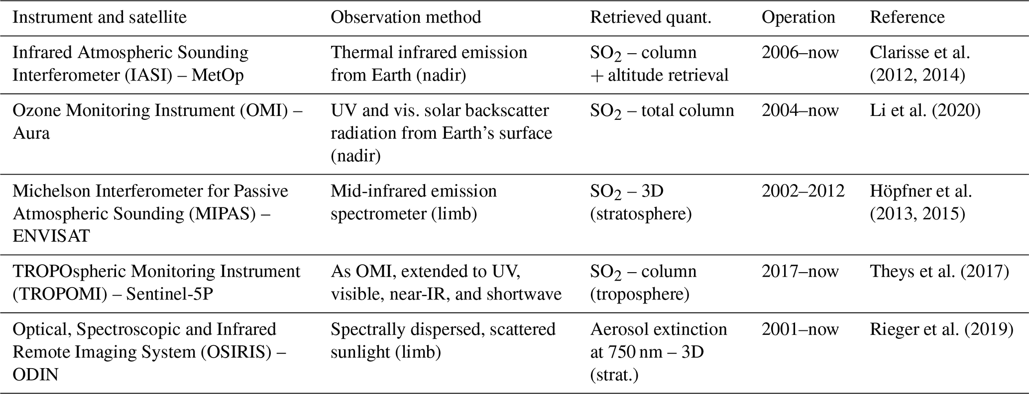
SO₂ and optical properties of aerosols in the atmosphere are continuously monitored by satellites. We use satellite observations of volcanic plumes for the evaluation of the new submodel, briefly summarized in Table 1. More details can be found in the provided references. Section 3.2 outlines which observations were used for which study. The versions of the datasets used are provided in the “Data availability” section.

Clarisse et al. (2012, 2014)Li et al. (2020)Höpfner et al. (2013, 2015)Theys et al. (2017)Rieger et al. (2019)

Table 1 Summary of satellite instruments and the respective observed quantities used for the evaluation of model simulations with the EVER submodel. More technical details in the observations and the applied retrievals can be found in the provided references.

Satellites typically do not directly observe the retrieved variables but rather functions of these variables, which rely on certain a priori information (Rodgers and Connor, 2003; Rodgers, 1990; Raspollini et al., 2006). Additionally, observed values are influenced by the horizontal and vertical resolutions used for retrieval, leading to contributions from neighbouring layers. To account for this effect, averaging kernel matrices (AKMs) can be applied to model data for comparison purposes. In this analysis, AKMs are used for comparisons with MIPAS observations. It is important to note that it is not possible to invert the AKM to correct the retrieved product.

3.2 EMAC model and experimental setup

We perform three separate numerical model experiments for the evaluation of the new submodel EVER and the established historic namelist setup. All simulations are performed with the ECHAM5/MESSy Atmospheric Chemistry (EMAC) model (Jöckel et al., 2006) that couples MESSy2 (Jöckel et al., 2010) to the general circulation model ECHAM5 (version 5.3.02; Roeckner et al., 2003). Temperature, the logarithm of the surface pressure, divergence, and vorticity are “nudged” (more details by  Jöckel et al., 2006; Jeuken et al., 1996) towards meteorological reanalysis data (ERA5; Hersbach et al., 2020) from the European Centre for Medium-Range Weather Forecasts (ECMWF) below 100 hPa. In addition, we employ the submodel for the simulation of the Quasi-Biennial Oscillation (QBO) to weakly nudge the simulations to QBO zonal wind observations between 10 and 90 hPa (Giorgetta et al., 2002) to avoid phase drift. Simulations are performed at T63 horizontal resolution for the simulation of stratospheric volcanic emissions and at T255 for the degassing case.

Gas-phase chemistry is addressed by the MECCA submodel (Sander et al., 2019). Details on the selected chemical mechanism in the different experiments are given below. Emissions from anthropogenic and biogenic sources and from biomass burning are introduced as described by Kohl et al. (2023). Sedimentation and dry and wet deposition are simulated using the submodels SEDI and DDEP (both Kerkweg et al., 2006) and SCAV (Tost et al., 2006), respectively. The namelist setup, chemical mechanism, and run script for the stratospheric (Sect. 4.1 and 4.2) and the Kilauea (Sect. 4.3) simulation can be found in the Supplement.

3.2.1 SO₂ in explosive volcanic eruptions – Nabro (2011)

First, we evaluate the EVER submodel and investigate the sensitivity of the resulting SO₂ plume to the injection parameters with the eruption of the Nabro volcano, starting on 13 June 2011 (Global Volcanism Program, 2011). The volcanic cloud predominantly comprised water and SO₂, reaching up to 20 km in altitude. As it was observed by a number of satellite instruments in contrast to the stronger eruption of Mount Pinatubo, it offers a perfect case study to investigate the spatio-temporal evolution of volcanic SO₂ in the stratosphere.

Figure 1 illustrates the evolution of the plume during the first days after the initial eruption, as observed from IASI and OMI. The top panel provides SO₂ height retrievals from IASI (Clarisse et al., 2014). The second and third row show retrieved SO₂ columns from IASI and OMI, respectively. SO₂ columns derived from IASI are presented only for coordinates where the retrieved SO₂ height exceeds 14 km, whereas OMI observes the total column. It is noteworthy that the precise timing of the satellite overpasses does not align for IASI and OMI observations.

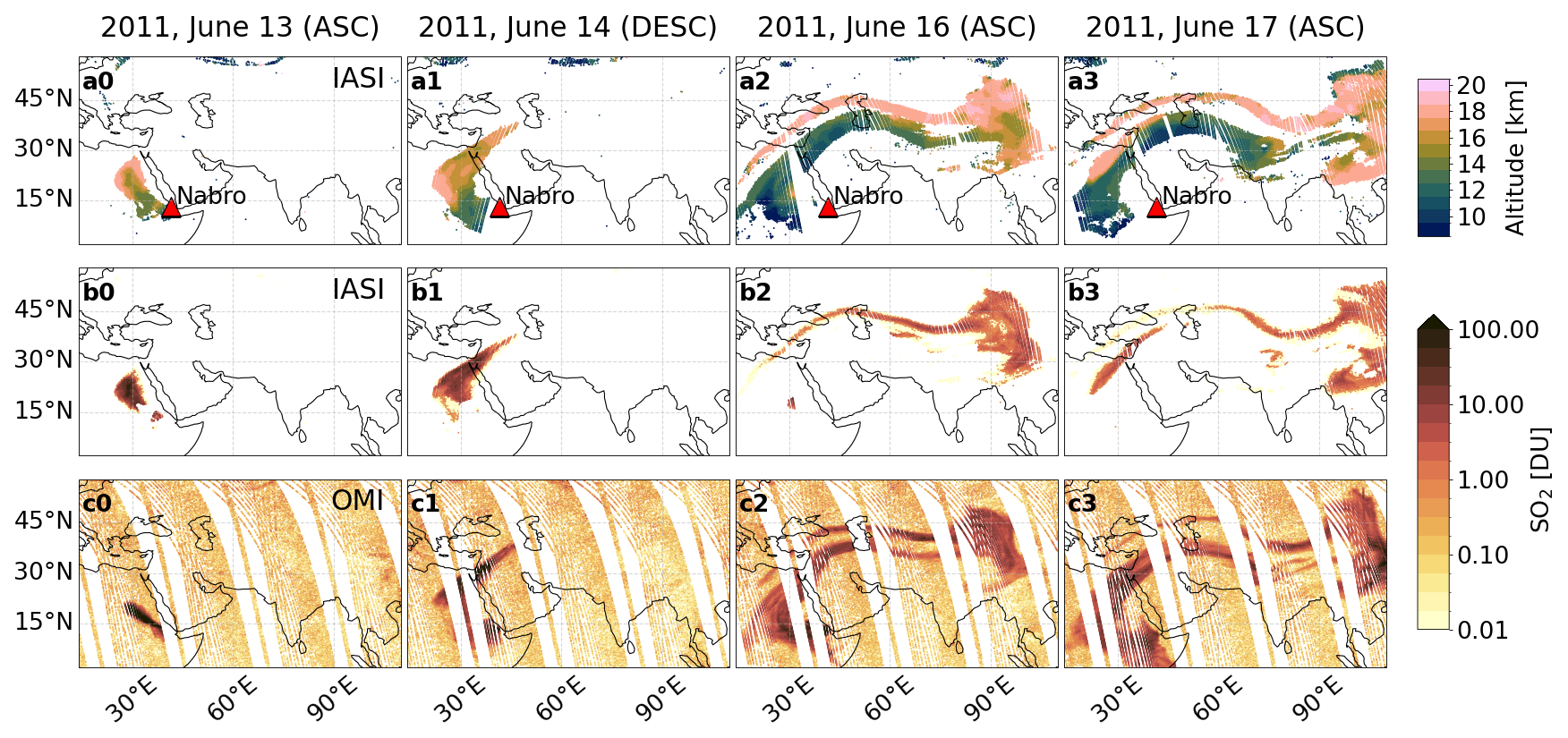
Figure 1 Observations of the Nabro plume on selected dates in the first week after the Nabro eruption. (a) SO₂ plume height retrievals from IASI satellite observations (Clarisse et al., 2014) during ascending (ASC) and descending (DESC) orbits. (b) Derived SO₂ columns from IASI (Clarisse et al., 2014) observations. (c) Derived SO₂ columns from OMI (Li et al., 2020) observations. IASI SO₂ columns are calculated assuming that all SO₂ is centred at the retrieved plume height (a0–a3), and we only display pixels where the retrieved SO₂ plume is detected in the stratosphere (above 14 km), whereas OMI displays the total column. Note that the timings of the observations do not coincide in general.

The initial stratospheric plume followed a northwestward trajectory during its ascent, entering the stratosphere at approximately 18° N, 30° E, and reached an altitude of up to 18 km (see Fig. 1a0, b0, c0). Within the UTLS, the SO₂ plume is influenced by the Asian monsoon anticyclone, subsequently evolving in a northeastward direction (Fig. 1a1, b1, c1). In the night of 15 to 16 June, an additional plume entered the stratosphere, as evident in the IASI observations from 16 June (Fig. 1a2). Concurrently, a wind shear within the AMA around the tropical tropopause induced a separation between tropospheric and stratospheric SO₂, with the stratospheric component further north (Fig. 1a2, a3). Subsequently, the SO₂ originating from the stratospheric entries mixed and was transported in the anticyclone. Approximately 10 d after the initial eruption, stratospheric SO₂ was distributed widely across the displayed region (not shown).

The difference between the stratospheric IASI SO₂ observations and OMI total columns confirms the altitude-specific findings depicted in the top panels of Fig. 1, enabling a distinction between tropospheric and stratospheric contributions to the total column. Furthermore, it highlights that while the Nabro volcano continuously emitted SO₂, plumes entered the stratosphere exclusively on 13 and 16 June. It is debated whether these stratospheric entries resulted from a direct injection caused by the eruption or whether the initial plumes failed to reach the stratosphere and were subsequently uplifted within the South Asian monsoon system (Bourassa et al., 2012b; Fromm et al., 2013; Vernier et al., 2013; Bourassa et al., 2013; Clarisse et al., 2014). Especially the second stratospheric plume on 16 June could comprise remnants of the tropospheric plume from 13 June that were uplifted. This study does not engage in this ongoing discussion but exclusively concentrates on the stratospheric entrance points of the plume.

For the Nabro eruption, we carried out a series of EMAC simulations to assess the sensitivity of stratospheric SO₂ burdens to varying emission source parameters. The simulations are performed at T63 horizontal resolution (approx. 190×190 km at the Equator), with 90 vertical levels up to 0.01 hPa and a model time step of 8 min. The SO₂ injection parameters of the reference simulation are based on the emission inventory developed by Schallock et al. (2023), refined with IASI observations (see below). We employed the Mainz Isoprene Mechanism version 1 (MIM1; Pöschl et al., 2000; Jöckel et al., 2016) within MECCA (see the Supplement for the detailed mechanism), considering oxidation of SO₂ with OH to form SO₃ and subsequently reacting with H₂O to form H₂SO₄. Carbonyl sulfide (OCS), a precursor for stratospheric aerosols, is constrained using monthly averaged surface concentrations as outlined by Montzka et al. (2007). Dimethyl sulfide (DMS) emissions from the ocean are computed using the MESSy submodel AIRSEA (Pozzer et al., 2006) and global ocean surface DMS concentrations derived by Lana et al. (2011) in the stratospheric setup.

The following simulations were performed:

• reference. This comprises the column emission centred at the altitude from the emission inventory minus 1 km (17 km); the Gaussian vertical distribution with a sigma of 2 km, confined to the altitude range from 16 to 18 km (see Sect. 2.1.2); horizontal position and timing derived from IASI (one column encompassing 22.9° N, 29.7° E, on 13 June 2011, 16:00–22:00 UTC); and the SO₂ amount (406 kt) from the emission inventory from Schallock et al. (2023).

• optimized. This is the same as the reference simulation but with the total amount distributed on two stratospheric entry points (67 % on 13 June and 33 % on 16 June based on the qualitative findings from the IASI observations).

• reduced. This is the same as the reference simulation but with reduced SO₂ emissions (280 kt).

• volc_pos. This is the same as the reference simulation but with emissions injected at the geographical location of the volcano (13° N, 41° E).

• point. This is the same as the reference simulation but using only one single grid box at the emission inventory altitude minus 1 km (17 km).

• min_2days. This is the same as the reference simulation but with emissions shifted by 2 d (11 June 2011, 16:00–22:00 UTC).

• plus_1km. This is the same as the reference simulation but with emissions shifted by 1 km in altitude (18 km).

• mills_et_al. These are emissions as described by Mills et al. (2016). The emissions are injected over several days and in columns covering the free troposphere and the UTLS region, ranging from 2.5 to 17 km. The only partly stratospheric emission takes place on 13 June, emitting 1500 kt and uniformly distributed over the altitude range from 9.7 to 17 km.

IASI observations of SO₂ columns and plume altitude are used for the qualitative evaluation of the short-term plume evolution (first week after the eruption; Sect. 4.1.1) by sampling simulated SO₂ columns at the time of the satellite's overpass using the SORBIT submodel (Jöckel et al., 2010). For the mid-term plume evolution and quantitative assessment of simulated SO₂ mixing ratios, we use three-dimensional observations from the MIPAS instrument³ (Sect. 4.1.2).

For the comparison with MIPAS observations, we calculate the stratospheric SO₂ burden, defined here as the sum over the SO₂ mass from lower integration limits depending on latitude (16 km for 0–30°, 14 km for 30–60°, and 12 km for 60–90°)⁴ up to 30 km altitude. We investigate the sensitivity of the model–observation agreement to the lower integration limit in Appendix A, showing changes in absolute values at similar agreement levels when varying the lower integration limit, thus justifying the usage of fixed lower integration limits for the evaluation.

3.2.2 Multi-year simulation with historic eruption namelist

To evaluate the new historic eruption namelist (EVER v1.1; see Sect. 2.2), we performed an EMAC simulation from January 2008 to December 2011, configured as detailed in Sect. 3.2.1. This time frame is characterized by high volcanic activity, including three strong eruptions – Kasatochi (August 2008), Sarychev (June 2009), and Nabro (June 2011) – alongside several smaller eruptions. Over the simulated 4 years, a total of 107 stratospheric injections from volcanic events are documented by Schallock et al. (2023) and considered in the simulation.

We use three-dimensional observations from the MIPAS instrument to evaluate the total stratospheric SO₂ burden (Sect. 4.2.1) with the same lower integration limit as described above. Whilst this study primarily focuses on the evaluation of simulated SO₂, this being the emitted species handled by EVER, we also present here the EMAC-simulated extinction and sAOD at 750 nm, evaluated with observations from the OSIRIS instrument (Bourassa et al., 2007, 2012a; Rieger et al., 2019) in the tropics (0–25° N, lower integration limit 16 km for the calculation of sAOD) and at higher northern latitudes (45–80° N, lower integration limit 12 km), as the tropopause altitude is fairly constant in these regions (Sect. 4.2.2). The additional evaluation of the simulated aerosol optical properties serves as a self-consistency check for the model; for context within the climate impacts of the resulting stratospheric aerosol; and as a comparison to the simulation done by Schallock et al. (2023), who used a similar setup.

Aerosol microphysics are treated with the submodel GMXe (Pringle et al., 2010). In our simulations, we apply four hydrophilic modes (nucleation, Aitken, accumulation, and coarse) and three hydrophobic modes (Aitken, accumulation, and coarse). We use the same GMXe setup as detailed in Schallock et al. (2023). Inorganic aerosol thermodynamics are treated with ISORROPIA-II (Fountoukis and Nenes, 2007), and sulfuric acid–water nucleation follows the parameterization by Vehkamäki et al. (2002). We calculate simulated aerosol optical properties of the GMXe aerosol populations with the AEROPT submodel (Dietmüller et al., 2016), providing extinction coefficients and the aerosol optical thickness of each model layer at various wavelengths.

3.2.3 SO₂ from a tropospheric degassing case – Kilauea (2018)

In addition to emissions from explosive volcanic eruptions, we evaluate the new submodel's capability to simulate emissions of degassing volcanoes by analysing a series of eruptive fissures at the Kilauea volcano in Hawaii, USA, in summer 2018 (Kern et al., 2020). SO₂ emissions from Kilauea have been studied with the EMAC model before for a different period (Beirle et al., 2014).

Simulations for the degassing case are performed at a horizontal resolution of T255 (approximately 50×50 km at the Equator) and 31 model levels (up to an altitude of about 30 km) to capture the tropospheric transport. For these simulations, we use a simpler chemical mechanism (compared to the T63 simulations) in the global model covering the basic tropospheric chemistry (as we do not focus on the stratosphere here), including O₃, OH, NO_x, NO_y, and basic sulfur chemistry (see the Supplement for details), to reduce the computational cost at this increased horizontal resolution and decreased time step of 2.5 min. Oxidation of SO₂ to H₂SO₄ is directly realized via reaction with OH in this simplified chemistry, without producing any intermediates. We do not consider DMS and OCS here (see the Supplement), leading to a potential underestimation of background maritime SO₂ concentrations.

The Kilauea SO₂ emissions are clearly observed from TROPOMI (ESA, 2018), serving as a basis for comparison with simulated columns. Jost (2021) derived daily SO₂ emission rates for Kilauea based on TROPOMI observations (SO₂ repro v1.1) and wind fields from ECMWF, using the divergence method developed by Beirle et al. (2019). Within this study, we use the original emission rates scaled up by a factor of 4.3 following recent updates, resulting in higher emission estimates. These adjustments include

• a.

  a factor of 3.2 due to non-linear effects caused by strong SO₂ absorption in the Kilauea volcanic plume (compare Theys et al., 2017) (while Jost, 2021, initially deemed this effect negligible, we included it after re-examination),

• b.

  a factor of 1.12 due to the change in the assumed plume height from 2000 to 1000 m (compare Kern et al., 2020),

• c.

  a factor of 1.19 from the consideration of topographic effects on the divergence calculation (Sun, 2022; Beirle et al., 2023).

To explore the potential for further emission optimization, we perform simulations with tuned SO₂ emission rates (see Fig. 9), based on the results of the reference simulation with the emission rates from Jost (2021). For that purpose, we establish a linear relationship between SO₂ emissions and simulated SO₂ by fitting the implemented emission rates of the 3 preceding days to the resulting simulated SO₂ columns on each day in June 2018 (the month of most intense SO₂ emissions), and we subsequently use this linear relationship to derive optimized emission rates resulting in the observed columns from TROPOMI, applying a stochastic gradient descent algorithm (e.g. Ruder, 2016). More details on the optimization can be found in Appendix B.

4 Evaluation and results

4.1 SO₂ in explosive volcanic eruptions – Nabro (2011)

4.1.1 Short-term SO₂ plume evolution

Figures 2 and 3 compare the simulated altitude of maximum SO₂ mixing ratios and SO₂ columns from the reference and sensitivity simulations to the corresponding IASI observations for the morning overpass on 14 June (1 d after the initial Nabro eruption) and the afternoon overpass on 17 June. SO₂ emissions in the simulation are confined to the stratosphere (except the approach by Mills et al., 2016), and thus only stratospheric amounts (altitude ≥ 14 km) are shown. Indeed, this approach neglects the significant amount of tropospheric SO₂ injected during the eruption. However, tropospheric SO₂ typically has a much shorter lifetime compared to stratospheric SO₂, which we focus on in this study. The reduced simulation is not shown in these figures, as it is equivalent to the reference simulation in altitude and only exhibits reduced columns.

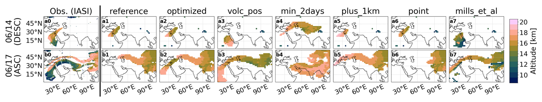
Figure 2 Derived plume altitude from the IASI satellite observations (a0, b0; compare Fig. 1) compared with the altitude of maximum SO₂ mixing ratios for each vertical column from the sensitivity simulations, 1 d (a0–a7) and 4 d (b0–b7) after the initial Nabro eruption. In the simulations, SO₂ was only injected into the stratosphere, except for in the mills_et_al simulation.

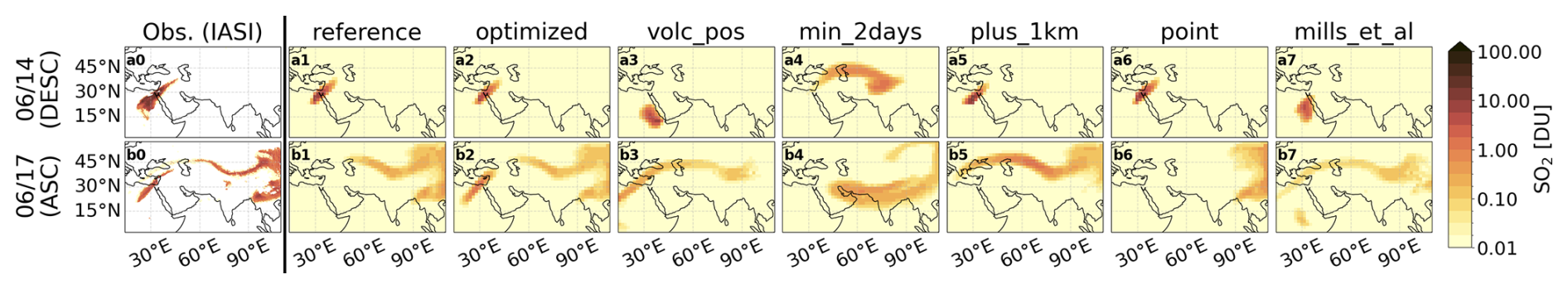
Figure 3 Column SO₂ derived from IASI satellite observations (a0, b0; compare Fig. 1) compared with the respective column from the sensitivity simulations, 1 d (a0–a7) and 4 d (b0–b7) after the initial Nabro eruption. In the simulations SO₂ was only injected into the stratosphere, except for in the mills_et_al simulation.

Overall, the simulated columns appear to be underestimated when compared to observations (see Fig. 3b). However, this might be attributed to the retrieval procedure of the column from the IASI observations. The column estimation assumes that all SO₂ of the plume is centred at the respective altitude depicted in Fig. 2. However, it takes into account the complete column, also including the tropospheric part of the plume. Hence, we only conduct a qualitative comparison between the simulated and observed column.

The reference simulation appears to reasonably capture the stratospheric evolution when considering only pixels where the altitude exceeds 14 km, although some discrepancies are evident. While the simulated altitude distribution horizontally broadens over time (Fig. 2b1), the total column analysis (Fig. 3b1) shows that the columns at the edges of the plume are very low, falling below the detection limit of IASI. Notably, as the reference simulation assumes only one stratospheric entrance, it fails to reproduce the observed second plume as expected (compare Fig. 3b0 and b1).

In the optimized simulation, the emissions are distributed across two space–time points, based on a detailed analysis of the IASI observations (refer to Fig. 1). As a result, the second plume is successfully reproduced, leading to better agreement with the observations (Fig. 3b2). By varying the geographical location of the stratospheric entrance (volc_pos), the plume encounters different meteorological patterns, resulting in a distinct evolution pattern. Similarly, adjusting the timing parameter (min_2days) leads to a more advanced evolution within the anticyclone (Fig. 3b4). These sensitivity analyses highlight the importance of accurately representing the timing and location of stratospheric injections for capturing the short-term evolution of volcanic plumes in atmospheric models.

As previously mentioned, a vertical wind shear leads to a displacement of the stratospheric part of the plume towards higher latitudes. Moreover, there appears to be a vertical gradient in wind speed above 16 km. When the emission altitude is increased by 1 km (plus_1km), the evolution within the anticyclone is attenuated (Fig. 2b5), suggesting lower wind speeds at higher altitudes. Additionally, the point simulation, where all emissions are centred at 17 km, only reproduces the rapid branch of the observed plume evolution. Consequently, it does not encounter the lower wind speeds experienced at higher altitudes (Fig. 2b6). In contrast, Mills et al. (2016) implemented emissions over several days and uniformly over altitudes ranging from 2.5 to 17 km, accounting for the continuous emissions that did not reach the stratosphere. However, in the mills_et_al simulation, stratospheric emissions are underestimated, leading to a substantial fraction of emissions being lost due to scavenging in the free and upper troposphere (Fig. 2b6).

4.1.2 Mid-term SO₂ mixing ratios

The zonal and 5 d averaged profiles of simulated and observed (MIPAS) stratospheric SO₂ mixing ratios on 16 July 2011, approximately 1 month after the eruption, are shown in Fig. 4 for the Northern Hemisphere. In addition to the sensitivity simulations discussed earlier, a simulation using 3D emission fields of SO₂ mixing ratios (3D_Schall in the following) is included for comparison (Schallock et al., 2023). These emission fields were derived from various satellite observations and applied several days after the initial eruption, specifically on 21 June for the Nabro eruption. Details on the methodology are described by Schallock et al. (2023). To simulate the effect of limited vertical resolution associated with MIPAS observations, the AKM (see Sect. 3.1) was applied to all simulated SO₂ mixing ratios.

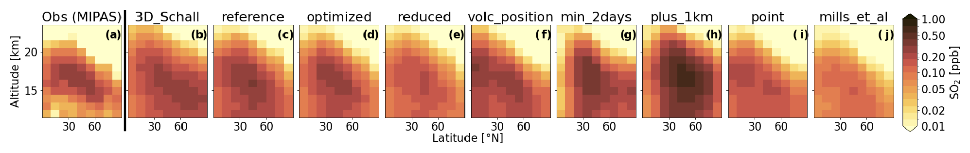
Figure 4 Zonally and 5 d averaged (14–18 July 2011) profile of northern-hemispheric stratospheric SO₂ mixing ratios derived from MIPAS observations (a) compared with the respective SO₂ mixing ratios simulated in the reference and sensitivity simulations 1 month after the eruption of the Nabro volcano.

The comparison between simulated and observed SO₂ distributions reveals some discrepancies, particularly in the vertical extent of the elevated SO₂ mixing ratios. The SO₂ distributions exhibit a slightly larger vertical extent compared to the observations. This discrepancy suggests a potential overestimation of the AKM or limitations in the vertical resolution of the simulation at the respective altitudes (approximately 500 m). The 3D_Schall simulation, which uses 3D emissions derived directly from satellite observations, shows the widest distribution (Fig. 4b). This discrepancy can be attributed to the fact that the 3D emissions already incorporate the smoothing effects introduced during the retrieval process (i.e. the AKM). Consequently, the simulated SO₂ mixing ratios in the 3D_Schall simulation represent observed mixing ratios rather than actual mixing ratios. Therefore, after applying the AKM to these simulated mixing ratios, the resulting altitude resolution appears to be too wide.

The sensitivity studies exhibit consistent patterns, with the highest mixing ratios of SO₂ typically observed between 15 and 20 km in altitude and 20° and 60° N in latitude and decreasing altitudes of the highest SO₂ mixing ratios with increasing latitude. The distribution follows the typical stratospheric circulation pattern and resembles the observed distribution. Lower mixing ratios compared to observations are found in the reduced, point, and mills_et_al simulations. In the reduced simulation, the reduced emissions directly lead to lower mixing ratios (Fig. 4e). However, in the mills_et_al simulation, a significant portion of SO₂ is removed in the upper troposphere, as discussed earlier (Fig. 4j). In the point simulation, restricting emissions to a single grid box omits the altitude range between 17 and 18 km, leading to a reduced stratospheric lifetime (Fig. 4i). Conversely, the plus_1km simulation shows higher mixing ratios due to the increased stratospheric lifetime associated with higher injection altitudes. The volc_pos (Fig. 4f) and min_2days (Fig. 4g) simulations exhibit slightly different spatial distributions, with the former indicating higher and the latter lower SO₂ mixing ratios at low latitudes. Hence, the varied meteorological conditions experienced in the initial days post-eruption consistently lead to diverse mid-term evolutions of stratospheric SO₂.

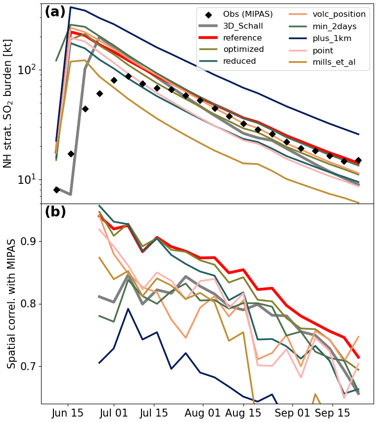
Figure 5 (a) The total northern-hemispheric (NH) stratospheric SO₂ burden as observed from the MIPAS satellite (black dots) and from the sensitivity simulations (5 d averages). (b) The spatial correlation in the latitude–altitude plane between the simulations and MIPAS observations, i.e. the spatial correlation between the first and all other panels in Fig. 4.

In addition to examining the spatial distributions at specific time points, we explored the mid-term changes in northern-hemispheric (NH) stratospheric SO₂ burden (Fig. 5a) and the mid-term spatial agreement between observed and simulated SO₂ mixing ratios (Fig. 5b) after the Nabro eruption. MIPAS observations of NH stratospheric SO₂ burden exhibit a gradual increase following the volcanic eruption, unlike the simulations, as discussed earlier. The 3D_Schall simulation's onset is delayed by a week, as the simulation is based on observations after the initial evolution of the plume in the stratosphere. The bottom panel of Fig. 5 illustrates the spatial correlation between the zonal profile of MIPAS observations and the sensitivity studies within the altitude–latitude window depicted in Fig. 4.

The stratospheric SO₂ burden of the reference, optimized, volc_pos, and min_2days simulations follows the same logarithmic decay, mostly coinciding with the observations after mid-July. These simulations also exhibit very similar spatial correlations, with some fluctuations, showing correlations around of 0.9 approximately 3 weeks after the eruptions, which gradually decrease to values between 0.75 and 0.8 in late September. The min_2days simulation shows a weaker correlation in the initial phase but approaches the others in the mid-term, most likely due to the different initial meteorological conditions.

The reduced, point, and mills_et_al simulations exhibit consistently lower stratospheric SO₂ mass as observed earlier, while the decay is parallel to the aforementioned. The spatial correlation of the reduced and point simulations is similar to that of the reference simulation, while the mills_et_al simulation shows a slightly smaller but comparable correlation. Emissions at higher altitudes (plus_1km) lead to higher SO₂ burden, longer lifetime, and lower spatial correlation with the observations. Initially, the simulation with three-dimensional emissions (3D_Schall) shows a total stratospheric SO₂ burden comparable to the reference simulation. However, it displays a slightly shorter lifetime as the burden decays more rapidly. Additionally, a slightly lower spatial correlation is observed, potentially attributed to the wider distribution of emissions.

The overall slightly faster decline in the stratospheric SO₂ burden in the simulation compared to the observations appears consistently across all simulations. It can be attributed to either an overestimation of the chemical removal, i.e. the oxidation with OH, or transport from the stratosphere to the troposphere that is too efficient, which also depends on the injection altitude and to a lesser extent the injection location.

4.2 Evaluation of the historic eruption namelist setup in a multi-year simulation from 2008 to 2011

4.2.1 Stratospheric SO₂ burden

Figure 6 illustrates total NH stratospheric SO₂ burdens, analogously to the upper panel of Fig. 5 for the simulated time frame from January 2008 to December 2011. We compare our simulation using the new EVER setup to the simulation from Schallock et al. (2023) using 3D emissions and observations from MIPAS.

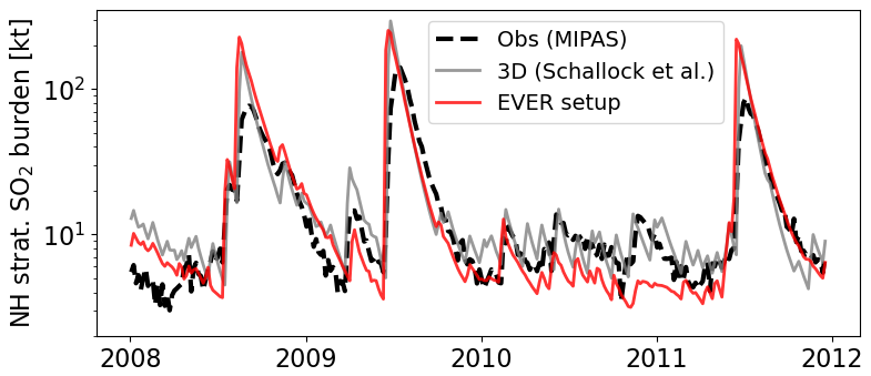
Figure 6 Timeline of total northern-hemispheric (NH) stratospheric SO₂ mass as observed from the MIPAS instrument (dashed black line) compared with simulations using the EMAC model with the new EVER historic volcanic setup (red) and using 3D emission fields (grey; Schallock et al., 2023).

The three primary peaks are largely reproduced similarly in both simulations, as anticipated, given that the injection mass from the emission inventory is derived from the 3D emission fields in the work of Schallock et al. (2023). However, in general, the observed peaks are lower than the simulated ones. This discrepancy can be attributed to the limited reliability of MIPAS observations shortly after strong eruptions (see Sects. 3.2.1 and 4.1.2 for details), underestimating actual SO₂ mixing ratios.

The EVER simulation exhibits an underestimation of background SO₂ mixing ratios, particularly evident during the relatively quiet period from the end of 2010 until the eruption of Nabro in June 2011, whereas the 3D simulation mostly reproduces the background mixing ratios. The discrepancy in the EVER setup is likely attributable to limitations in the general model configuration or the overestimation of the vertical extent of the emissions for smaller eruptions, only reaching the tropopause. Future efforts will concentrate on enhancing the representation of background SO₂ and aerosol in both the free and the upper troposphere, as well as in the stratosphere. However, it is worth noting that the simulation does reproduce smaller volcanic events, albeit at reduced magnitudes. As previously discussed, these smaller injections are not optimized in terms of horizontal position and timing, as they fall below the detection limit of IASI.

4.2.2 Optical properties of the resulting stratospheric aerosol

The main focus of the observational evaluation of EVER is on the spatio-temporal evolution of volcanic SO₂ as the emitted species. However, once in the atmosphere, the SO₂ can be converted into sulfur aerosol particles, with e-folding times varying between 2 and 40 d (Carn et al., 2016; Höpfner et al., 2015). For additional validation and a comparison to the simulation performed by Schallock et al. (2023), we compare the optical properties of the resulting stratospheric aerosol to observations from the OSIRIS instrument.

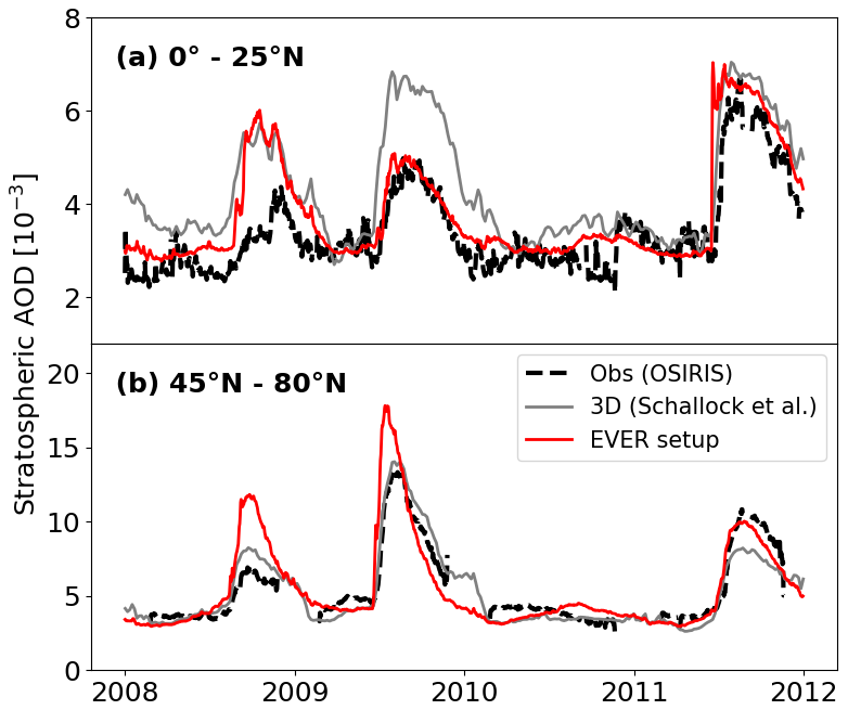
Figure 7 Timeline of sAOD at 750 nm (for the vertical range of the integration, see Sect. 3.2.2) as observed from the OSIRIS instrument (dashed black line) compared with simulations using the EMAC model with the new EVER historic volcanic setup (red) and with 3D emission fields (grey; Schallock et al., 2023). The sAOD is evaluated in the northern-hemispheric tropical latitudinal band from 0 to 25° N (a) and at higher northern latitudes from 45 to 80° N (b).

Figure 7 shows the sAOD for the 4 simulated years, categorized into two regions: the NH tropics (0 to 25° N) and the middle to higher latitudes in the Northern Hemisphere (45 to 80° N). In both regions, the three major peaks corresponding to the volcanic eruptions are evident. Discrepancies between the EVER simulation and observations are expected in regions where the stratospheric injection occurred, attributable to cloud overlap and saturation effects in the observations. This discrepancy is observed for Kasatochi (2008) and Sarychev (2009) at higher latitudes and for Nabro at lower latitudes. Conversely, the 3D emissions, directly derived from satellite observations and applied with a delay, reproduce these measurement biases.

In the aftermath of the Nabro eruption in June 2011, the sAOD in the EVER simulation exhibits a sharp increase followed by notable fluctuations. The fluctuations can be attributed in part to the movement of the plume centre across the 25° latitude band, resulting in variable alignment with the observed latitude window. The fluctuations could also be a consequence of microphysical processes that are outside of the scope of the paper. Notably, the observations show similar fluctuations in the following days.

Another interesting feature is the pronounced overestimation of sAOD in the tropical latitudes following the Kasatochi eruption. This anomaly could be attributed to an overestimation of transport from higher latitudes to the tropical stratosphere or to a general overestimation of the emissions. Notably, this feature is not observed after the Sarychev eruption in the EVER simulation, although it is present in the 3D simulation. The discrepancies between the two simulations in the mid-term transport after the Sarychev (to the tropics) and Nabro (to high latitudes) eruptions may be attributed to the different timings of the emissions. While emission times in the EVER simulation were optimized to the first detection of stratospheric SO₂ from the IASI satellite, 3D emissions were applied on the dates specified in Schallock et al. (2023). The interaction with the South Asian monsoon anticyclone potentially causes differing transport to lower or higher latitudes if the altitude, timing, and geographical location of the emission do not coincide.

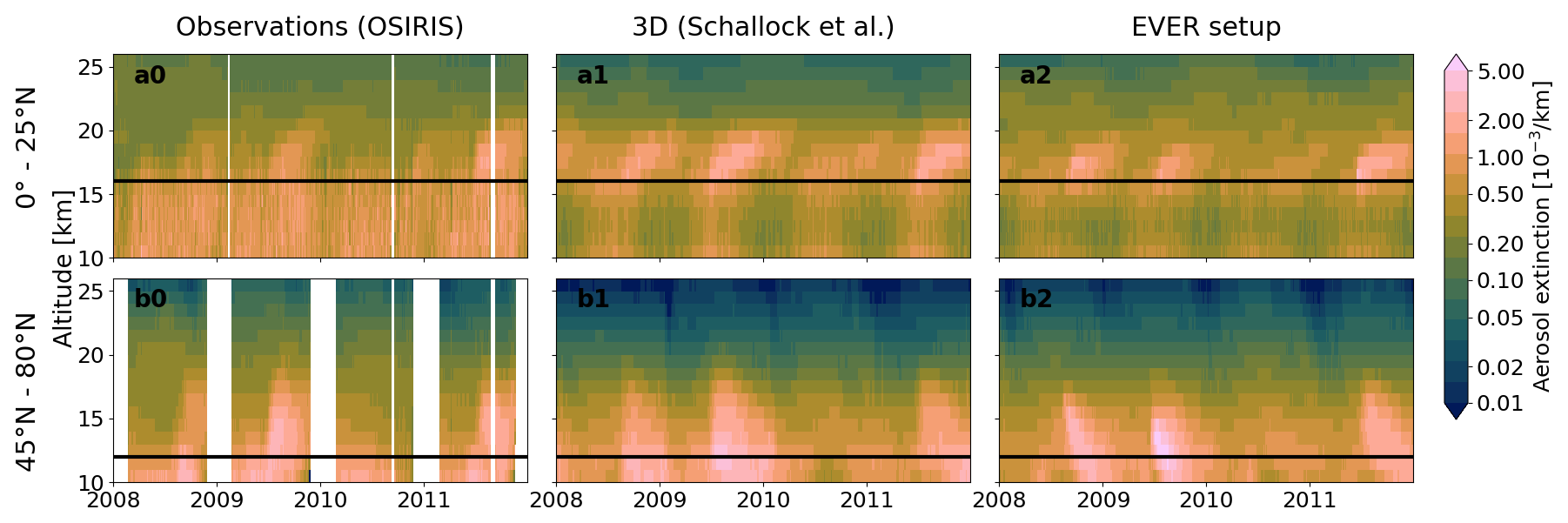
Figure 8 Timeline of aerosol extinction at 750 nm as observed from the OSIRIS instrument (a0, b0) and simulated by the EMAC model using 3D emissions (a1, b1; Schallock et al., 2023) and using the new EVER historic volcanic setup (a2, b2), evaluated in the northern-hemispheric tropical latitudinal band from 0 to 25° N (a) and at higher northern latitudes from 45 to 80° N (b).

Figure 8 displays the aerosol extinction at 750 nm, as observed from the OSIRIS instrument and simulated. The effect of the three major volcanic eruptions is mostly evident between 16 and 20 km in the tropics and between 12 and 18 km at higher latitudes. Similarly to Fig. 7, the magnitude of extinction differs between the observations and the two simulations. In addition, discrepancies are noticeable in the maximum altitude of the plume and below the tropopause. While the 3D simulation largely reproduces the observed maximum altitude, using satellite observations with, in the case of MIPAS, the incorporated AKM as input, the EVER simulation may present more realistic maximum altitudes. The differences between the observations and the simulation below the tropopause are strongly driven by the coincidence with clouds which hinder the retrieval of aerosol extinction. The slight differences between the two simulations from 10 to 15 km in the tropics can most likely be attributed to the differences between the simulation setups. In addition, the QBO signal with differing aerosol concentrations above 20 km, depending on the QBO phase (e.g. Hommel et al., 2015), is more pronounced in the simulation, potentially subject to future studies.

In the sensitivity simulations from Brodowsky et al. (2021), the emission database from Brühl et al. (2018) consistently showed the lowest stratospheric aerosol amounts compared to the other emission databases, in poor agreement with observations. However, we show much better agreement with observations in our simulations and see even higher SO₂ mixing ratios when applying the emission inventory of (Schallock et al., 2023, extension of Brühl et al., 2018) compared to the emission database from Mills et al. (2016). This contradiction can be attributed to the vertical extent of the emission. In Brodowsky et al. (2021), “the emitted SO₂ plume is assumed to be evenly distributed [from] the given plume top downwards one third of the way to the Earth's surface”, which would mean a vertical extent of 12 to 18 km for the Nabro volcano. While this approach seems reasonable for the databases of Diehl et al. (2012) and Carn et al. (2017), as they consider the tropospheric and stratospheric part of the plume, it leads to a vast underestimation of the stratospheric SO₂ when applied on the stratospheric emissions by Brühl et al. (2018). In this study, SO₂ is emitted between 16 and 18 km for the Nabro volcano in our simulations.

4.3 SO₂ from degassing volcanoes – Kilauea (2018)

In the following, we investigate the degassing event at Kilauea. Figure 9 depicts a comparison between observed columns from TROPOMI in the top row (a) and simulated columns from the simulations with derived emission rates from Jost (2021) (“Jost2021”, row b) and with optimized emission rates (“optimized”, row c). Generally, SO₂ columns are highest in proximity to the Kilauea volcano and disperse according to meteorological conditions. Qualitatively, we observe reasonable agreement in the horizontal dispersion of the plume on most days (Fig. 9), with some exceptions, such as 7 and 10 June. However, there is stronger variability in the observations within the transported plume compared to the simulations, where we predominantly observe gradually decreasing SO₂ columns with distance from the volcano. This effect is attributed to the diurnal variability in the SO₂ emissions, which are not represented in the emission dataset.

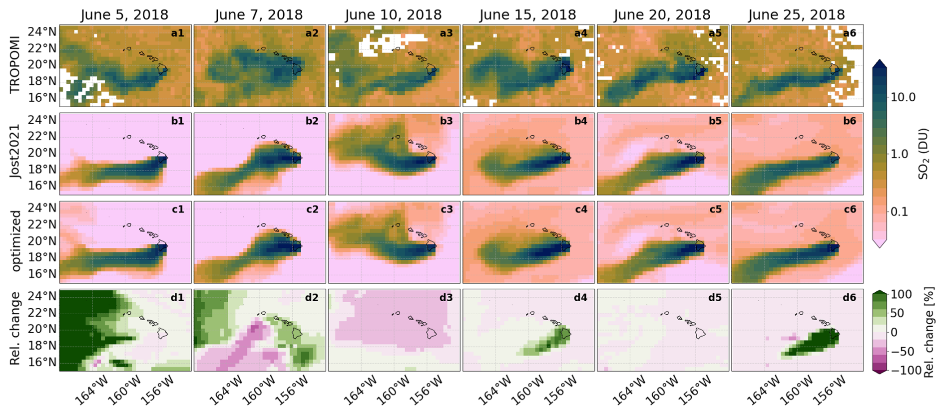
Figure 9 Observed (a1–a6) and simulated SO₂ columns resulting from the degassing of the Kilauea volcano on selected days in June 2018 at a model resolution of T255. (a) Observations from TROPOMI, regridded to T255 resolution. (b) Simulation with emission rates derived by Jost (2021, scaled by a factor of 4.3 – see text for details). (c) Simulation with optimized emission rates, based on a comparison between model and observations (refer to the text for more details). (d) Relative change from the simulation with derived emission rates by Jost (2021) to the optimized simulation.

Figure 10 provides a quantitative assessment of the horizontal extent depicted in Fig. 9 (spanning 168 to 152° W, 15 to 25° N), showing (bottom) spatially averaged SO₂ columns within this horizontal window, $\stackrel{\mathrm{‾}}{{{\mathrm{SO}}_{\mathrm{2}}}_{(\mathtt{\text{col}},d)}}$, as observed and simulated at each day in June 2018, d, and (top) spatial correlation between simulated and observed logarithmic SO₂ columns within this horizontal window. The Jost2021 numerical results exhibit some noticeable fluctuations in $\stackrel{\mathrm{‾}}{{{\mathrm{SO}}_{\mathrm{2}}}_{(\mathtt{\text{col}},d)}}$, with periods of underestimation in the initial days and on 25 June, as well as instances of significant overestimation, such as on 11 and 21 June. The presence of a low bias can be primarily attributed to missing or very low emissions from Jost (2021) due to missing orbits or cloud cover hindering reasonable SO₂ retrieval. As expected, the simulated $\stackrel{\mathrm{‾}}{{{\mathrm{SO}}_{\mathrm{2}}}_{(\mathtt{\text{col}},d)}}$ from the optimized simulation follows the observed pattern much more closely as a result of the tuning.

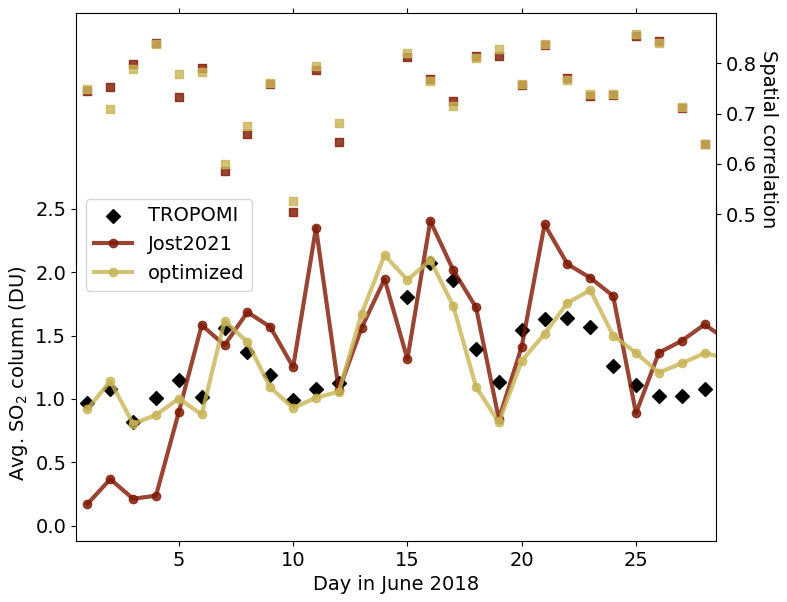
Figure 10 Derived spatially averaged SO₂ column from TROPOMI observations (168 to 152° W, 15 to 25° N; horizontal window displayed in Fig. 9) in June 2018 compared with simulations, using emission rates from Jost (2021, scaled by a factor of 4.3 – see text for details) and optimized emission rates, based on a comparison between model and observations. At the top, we present spatial correlations in the same horizontal window between the observations and the respective simulations, using the same colour as for the SO₂ column.

On most days, a strong spatial correlation between the simulated and observed horizontal dispersion of the SO₂ plume is evident, ranging from 0.6 to 0.9. However, the pronounced exceptions on 7 and 10 June (also depicted in Fig. 9) may be attributed to misrepresentations of the meteorological conditions or generally lower wind speeds, leading to more turbulent flow. Barely any improvement in spatial correlation can be observed from the Jost2021 simulation to the optimized one. This lack of difference is primarily due to the intra-day fluctuations in SO₂ emissions, which contribute to the observed variations and are also not accounted for in the optimized simulation, and to potential differences in injection height that are not considered in the simulation. To address the former, emission rates would need to be implemented at higher temporal resolution (e.g. hourly) and simulations performed at higher horizontal resolution.

5 Discussion

We showed that SO₂ emissions from explosive volcanic eruptions and the subsequent plume evolution can be reasonably reproduced in EMAC within the MESSy model system, using either 3D emissions (Schallock et al., 2023) derived from satellite observations or column emissions with differing vertical profiles. The different approaches exhibit strengths and weaknesses and reveal information about the general capabilities of the model.

The usage of 3D emissions, as investigated by Schallock et al. (2023), offers significant advantages for assessing the mid- and long-term impact of volcanic eruptions. By directly deriving emissions from 3D satellite observations several days after the initial eruption, this approach ensures an accurate representation of the plume's horizontal and vertical evolution, particularly during the crucial initial phase post-eruption, which is heavily influenced by local meteorological conditions. However, a notable drawback of this method is the inherent limitation to the vertical sensitivity of the satellite observations, leading to an overestimation of the vertical extent of the plume and thus not reproducing the real distribution. Consequently, this discrepancy impacts the plume's subsequent evolution and results in differing stratospheric lifetimes for the volcanic plume. Additionally, due to the reliance on 3D satellite observations and the delayed injection, short-term volcanic effects cannot be adequately examined for the simulation with 3D emissions. Another limitation of the approach outlined by Schallock et al. (2023) lies in its technical implementation, which necessitates manual addition of retrieved tracer perturbations and subsequent model restarts after each volcanic event or the use of large import files, posing practical challenges for operational use.

Column emissions rely on several assumptions regarding critical parameters such as the plume height and location, emitted mass, and emission profile. With sufficient observational data, these parameters can be effectively constrained, enabling accurate predictions of SO₂ mixing ratios. However, the creation and updating of such inventories also need manual work, retrieving the relevant parameters. As demonstrated with the Nabro volcano, we used data from the volcanic SO₂ emission inventory compiled by Schallock et al. (2023) in combination with observations from IASI to accurately constrain these parameters. Consequently, our model simulations exhibited strong agreement with both short- and mid-term observations of SO₂ mixing ratios and aerosol optical properties obtained from the IASI, MIPAS, and OSIRIS satellite instruments, specifically evaluated for strong eruptions.

The sensitivity studies revealed that the importance of accurately constraining the emission parameters for adequately simulating the volcanic SO₂ plume differs for each parameter. Primarily, emitting an appropriate quantity of SO₂ at the correct altitude appears to be the most critical factor. Variations in the SO₂ amount directly influence stratospheric SO₂ mixing ratios, with the mixing ratios approximately proportional to the mass emitted. Conversely, discrepancies in the injection altitude substantially impact the stratospheric lifetime of the resulting SO₂ and sulfur aerosol, as well as the meteorological conditions encountered by the plume.

For that reason, we opted for Brühl et al. (2018) for the emission database and Schallock et al. (2023) for the historic default namelist setup, as they specifically target SO₂ injections above the tropopause, while the databases from Diehl et al. (2012) and Carn et al. (2017) do not distinguish between the tropospheric and stratospheric part of the plume and provide no information about the SO₂ amount above the tropopause. Mills et al. (2016) do provide a minimum and maximum plume altitude but potentially underestimate the stratospheric part when uniformly emitting over this altitude range, as can be seen in the sensitivity study on the Nabro volcano (see Sect. 4.1.2). The unclear stratospheric contribution of the initial SO₂ emission is also the main reason for the vastly differing stratospheric sulfur burden estimated by Brodowsky et al. (2021) from the different emission databases, again highlighting the importance of the correct retrieval and application of the stratospheric part of the plume. The emission database from Schallock et al. (2023) additionally explicitly includes smaller eruptions reaching the stratosphere.

However, column or point emissions come with inherent limitations as well. First, emissions are constrained to a single grid box or columns of grid boxes in this study. In detailed studies of strong eruptions, we additionally recommend exploring the effects of emissions over multiple columns and an extended time period to avoid non-linearities due to very high local concentrations (see also Sect. 2.1.2). Second, volcanic activity typically extends beyond a single day, with SO₂ emissions occurring over prolonged periods, occasionally reaching the stratosphere (see Sect. 4.1 for the Nabro eruption). While related discrepancies dissipated in the mid-term for the Nabro volcano, this may not necessarily be the case for other volcanic eruptions. Third, the exact timing and geographical location of the stratospheric entry point cannot always be accurately estimated. Our sensitivity analyses uncovered short- and mid-term disparities when such information was lacking.

Based on the insights from the sensitivity studies, we developed a historical namelist configuration for the new EVER submodel spanning the past 3 decades. Despite the aforementioned limitations, our evaluation simulation demonstrates a satisfactory alignment with observations of both SO₂ mixing ratios and aerosol optical properties. Notably, the historic namelist setup accurately reproduces significant eruptions, thereby representing the primary contribution of volcanic events to the stratospheric SO₂ and aerosol loading. This aligns with our conclusion that altitude and mass, which were directly determined from the emission inventory and do not depend on the availability of IASI observations, are the most crucial emission parameters. However, we showed that the timing and geographical location of the stratospheric entry point can lead to additional uncertainties that remain when no IASI observations are available.

Consequently, we recommend the adoption of the submodel EVER with the proposed historical namelist setup (see Sect. 2.2 and the Supplement) in all numerical simulations using the MESSy framework at global or regional scale, particularly those encompassing the stratospheric and upper-tropospheric domains. This is the first study to systematically incorporate volcanic eruptions into atmospheric simulations within MESSy using the EMAC model, presenting a more flexible and easier-to-implement alternative to the 3D emission approach. Furthermore, in cases where disparities with observations arise, owing to the aforementioned uncertainties, or when focusing on specific volcanic events, the namelist setup can be adjusted accordingly, especially regarding the horizontal and vertical extent of the plume. Moreover, comparisons with simulations using 3D emission fields may offer additional insights into the evolution of individual volcanic plumes.

In Sect. 4.3, we demonstrated the additional capability of EVER to simulate SO₂ from degassing volcanoes. However, it is essential to apply a model with a sufficiently finely resolved horizontal grid (for a global model) to accurately capture the observed phenomena and the small-scale wind fluctuations. Simulations with equal emissions performed at more standard horizontal resolutions, such as T63 and T106, failed to reproduce the observations adequately (not shown), whereas these resolutions are mostly sufficient for stratospheric simulations. Furthermore, we applied model-driven tuning for the corresponding emission rates, reproducing observed SO₂ column amounts.

This optimization has the potential to be extended to historic degassing volcanoes, facilitating the development of a default setup akin to the stratospheric default setup for explosive volcanoes. This process would include integrating TROPOMI observations with an initial simulation using rough estimates of degassing emissions, which could subsequently be refined through stochastic gradient descent (SGD) optimization as described in Appendix B, potentially extending or replacing the outdated climatology by Diehl et al. (2012) used in many EMAC simulations. However, implementing this approach may encounter challenges related to the required high horizontal resolution, the estimation of the injection altitude, and the identification and initial approximate estimation of all significant degassing volcano emissions.

Up to this point, our focus has been primarily on volcanic SO₂. However, it is worth mentioning the versatility of the submodel for a wide range of use cases where gaseous or aerosol tracers are injected into the atmosphere in vertical distributions, with limited horizontal extent. This includes the following use cases:

• Volcanic ash. Apart from emitting trace gases, volcanic eruptions also release primary aerosols, such as volcanic ash. The EVER submodel is explicitly designed to simulate the evolution of aerosol species, including volcanic ash, after volcanic eruptions.

• Water vapour. Eruptions of submarine volcanoes, such as the notable event at Hunga Tonga-Hunga Ha'apai in January 2022 (e.g. Vömel et al., 2022; Sellitto et al., 2022; Schoeberl et al., 2022; Xu et al., 2022), release substantial quantities of water vapour into the atmosphere. The EVER module can be used to investigate the effects of enhanced water vapour concentrations in the stratosphere due to volcanic activity. For the Hunga Tonga eruption, we recommend the simultaneous injection of water vapour in multiple columns to avoid quick removal by ice formation and to be consistent with observations.

• Wildfires. Strong wildfires can inject significant quantities of carbonaceous aerosols and various trace gases directly into the stratosphere via pyro-cumulonimbi. EVER can be used to model these emissions from wildfires.

• Solar radiation modification. Studies on solar radiation modification, particularly artificial injections of SO₂ or other trace gases into the stratosphere to form aerosols that reflect sunlight back into space, can benefit from the capabilities of EVER. These scenarios involve large uncertainties, which can be addressed with studies using EVER.

• Transport processes. Transport processes play a crucial role throughout the atmosphere. EVER allows for the emission of active and passive aerosols and trace gases throughout the atmosphere, enabling the study of processes such as the exchange between the troposphere and stratosphere.

• Sensitivity studies. Atmospheric properties can be highly sensitive to perturbations in trace gas or aerosol mixing ratios. By injecting the respective atmospheric constituents with EVER, it is possible to estimate the sensitivity of climate, atmospheric dynamics, and the ozone column to these perturbations.

6 Conclusions

We presented the new submodel for tracer emissions from Explosive Volcanic ERuptions (EVER v1.1), developed within the Modular Earth Submodel System (MESSy, version 2.55.1), and performed numerical experiments with the ECHAM5/MESSy Atmospheric Model (EMAC) and the new submodel.

EVER is designed for the addition of gaseous and aerosol tracer tendencies following volcanic eruptions in columns with user-specified vertical profiles at point or area sources. We evaluated the EVER submodel with the simulation of volcanic SO₂ emissions in the EMAC model for the explosive eruption of Nabro in June 2011 and a degassing event from Kilauea in July 2018, employing satellite observations from IASI, MIPAS, OMI, TROPOMI, and OSIRIS. The evaluation showed that volcanic emission plumes can be reasonably simulated with EVER. The new submodel is available from MESSy version 2.55.1 and will be continuously developed further.

We investigated the sensitivity of the volcanic SO₂ plume evolution after the Nabro eruption to variations in the emission parameters. The results emphasized the importance of the emission of a reasonable amount of SO₂ above the tropopause with an appropriate altitude distribution. In previous studies with various emission databases, the SO₂ mass emitted in the stratosphere was unclear, resulting in large differences. We showed that the application of a dedicated stratospheric SO₂ emission inventory can reproduce observed SO₂ burdens and aerosol optical properties. Horizontal position and emission timing were found to have a minor impact on the mid-term SO₂ burden in the stratosphere. Nevertheless, these parameters play a crucial role in detailed process studies during the initial weeks after an eruption.

Furthermore, we conclude that simulations of volcanic eruptions can be effectively performed with the help of 3D emissions and column emissions if the emitted stratospheric SO₂ mass is well constrained. However, both approaches have shortcomings. The optimal approach depends on the specific use case, with column emissions excelling in the short-term and similar performance in the mid-term to long term.

Finally, we developed a historic submodel setup for EVER, incorporating stratospherically significant volcanic eruptions spanning 1990 to 2023. It is based on the volcanic SO₂ emission inventory by Schallock et al. (2023). We additionally optimized the timing and geographical location of the volcanic plume entering the stratosphere, using the findings of the sensitivity study and SO₂ observations from the IASI satellite. However, this information was only available from 2007 on and for strong volcanic eruptions only. The historic namelist setup was successfully evaluated with regard to resulting SO₂ mixing ratios and aerosol optical properties. It is provided in the Supplement, and we advocate its inclusion in simulations using the MESSy framework focusing on the upper troposphere and the stratosphere. For very strong eruptions, it may be beneficial to distribute the emissions over multiple columns horizontally and an extended time period or to adjust the vertical plume extent if discrepancies with observations occur.

In addition to the extensively discussed application to explosive volcanic eruptions, the EVER submodel's versatility opens up a range of additional research opportunities. These may include investigations into the interplay between SO₂ and volcanic ash post-eruption, exploration of solar radiation modification scenarios, modelling of wildfires, and analyses of atmospheric transport processes. Future work could involve the development of a climatology of SO₂ emissions from degassing volcanoes employing the new submodel.

Appendix A: Sensitivity of the evaluation results to the lower integration limit for the calculation of stratospheric properties

As the tropopause does not necessarily coincide in the simulation and the observations, we applied latitude-dependent fixed-altitude lower integration limits for the calculation of stratospheric SO₂ burden and sAOD. Here, we study the sensitivity of the evaluation results to the chosen lower integration limit.

The stratospheric SO₂ burden is defined in this work as the SO₂ mass above 16 km from 0–30°, above 14 km from 30–60°, and above 12 km from 60–90°. We compare these stratospheric SO₂ burdens to burdens with perturbed lower integration limits (+1 km: 17, 15, 13 km; −1 km: 15, 13, 11 km). The results are depicted in Fig. A1. While the total burden varies in the three scenarios as expected, the agreement between the simulations and the observations is very similar, especially considering the three major volcanic peaks. However, in the quiet period in 2010 and 2011, the agreement improves, when the lower integration limit increases (Fig. A1b). This can be attributed either to an incorrect altitude distribution of the background SO₂ or to the emission of the smaller eruptions.

The sAOD is defined here as the integral over the aerosol extinction above 16 km from 0–25° and above 12 km from 45–80°. As before, we vary this lower integration limit by ±1 km (see Fig. A2). Again, we see similar agreement at differing absolute values. The strongest difference can be seen in the Sarychev peak at higher latitudes (Fig. A2e), which seems to be underestimated when increasing the lower integration limit. This might be connected to either the missing AKM or the plume top being underestimated.

Overall, we conclude that our evaluation results are not very sensitive to the chosen lower integration limit for the calculation of the stratospheric SO₂ burden and the sAOD. Thus, the evaluation results are mostly independent of the chosen tropopause definition.

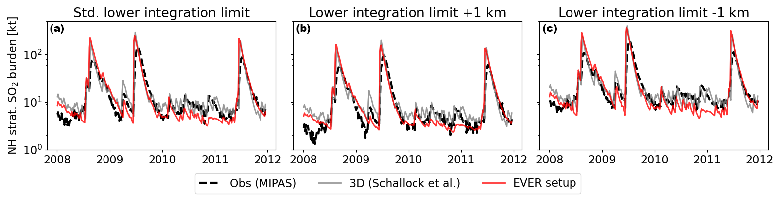
Figure A1 Sensitivity of the evaluation results to the lower integration limit (applied to observations and simulations) for the derivation of the stratospheric SO₂ burden. (a) Lower integration limit as applied in the paper (16 km from 0–30° N, 14 km from 30–60° N, and 12 km from 60–90° N). Variations of plus 1 km (b) and minus 1 km (c), showing similar agreement at different absolute values. Slight differences can be seen at background levels, with increased agreement in 2010 for the increased lower integration limit (b).

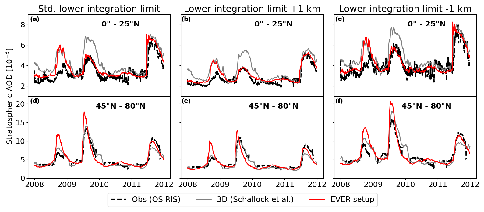
Figure A2 Sensitivity of the evaluation result to the lower integration limit (applied to observations and simulations) for the derivation of sAOD. (a, d) Lower integration limit as applied in the paper (16 km from 0–25° N and 12 km from 45–80° N). Variations of plus 1 km (b, e) and minus 1 km (c, f), showing similar agreement at different absolute values. The most significant differences are observed for the Sarychev volcano, which shows strongly decreased simulated sAOD at an increased lower integration limit at higher latitudes (e).

Appendix B: Optimization of the emission rates from the Kilauea degassing event

In Sect. 4.3, we optimized the emission rates of the Kilauea volcano such that the model reproduces the observed average SO₂ column $\stackrel{\mathrm{‾}}{{{\mathrm{SO}}_{\mathrm{2}}}_{(\mathtt{\text{col}},d,\mathtt{\text{obs}})}}$ for each day d over the chosen area. Here, the optimization is described in more detail.

In the first step, we investigated the relation between the implemented emission rates and resulting simulated $\stackrel{\mathrm{‾}}{{{\mathrm{SO}}_{\mathrm{2}}}_{(\mathtt{\text{col}},d,\mathtt{\text{sim}})}}$. Therefore, we considered the emission rates from the 3 preceding days of each sampled day in June 2018, denoted as emis${}_{{\mathrm{SO}}_{\mathrm{2}};d-i}(i=\mathrm{0},\mathrm{1},\mathrm{2})$, and constructed a linear predictor of $\stackrel{\mathrm{‾}}{{{\mathrm{SO}}_{\mathrm{2}}}_{(\mathtt{\text{col}},d)}}$:

$$\begin{array}{}\text{(B1)}& \stackrel{\mathrm{‾}}{{{\mathrm{SO}}_{\mathrm{2}}}_{(\mathtt{\text{col}},d,\mathtt{\text{sim}})}}={{\mathrm{SO}}_{\mathrm{2}}}_{\left(\mathtt{\text{col,BG}}\right)}+\sum _{i=\mathrm{0}}^{\mathrm{3}}{a}_{d-i}\cdot {\mathrm{emis}}_{{\mathrm{SO}}_{\mathrm{2}};d-i}.\end{array}$$

The coefficients a_d−i, representing the importance of the emissions of each of the 3 preceding days, respectively, and the background SO₂ column amount, ${{\mathrm{SO}}_{\mathrm{2}}}_{\left(\mathtt{\text{col,BG}}\right)}$, are the free parameters in the linear predictor and were determined through a least-squares fit. Subsequently, the linear predictor with these coefficients was utilized to compute optimized emission rates for each day using a stochastic gradient descent (SGD) algorithm, iteratively optimizing the emission rates by reducing the loss function (e.g. Ruder, 2016). The optimization scheme is given in pseudocode in Algorithm B1.

Algorithm B1 SGD optimizer for daily SO₂ emission rates

Require:

niter,lrate

1:

while j<niter do

2:

for d=0,d<30,k++ do

3:

for k=0,k<3,k++ do

4:

gradient=2*ad-k⋅(SO2(col,dobs) $\mathrm{-}{\mathrm{\sum }}_{\text{i=0}}^{\text{2}}$ ad-i⋅emis${}_{{\text{SO}}_{\text{2}}\mathrm{;}\text{d-i}}\mathrm{-}$SO2(col,BG))

5:

emis${}_{{\text{SO}}_{\mathrm{2}}\mathrm{;}\text{d-k}}$+=lrate*gradient

6:

end for

7:

end for

8:

j++

9:

end while