Knowledge-inspired fusion strategies for the inference of PM_2.5 values with a neural network

Ground-level concentrations of particulate matter (more precisely PM_2.5) are a strong indicator of air quality, which is now widely recognised to impact human health. Accurately inferring or predicting PM_2.5 concentrations is therefore an important step for health hazard monitoring and the implementation of air-quality-related policies. Various methods have been used to achieve this objective, and neural networks are one of the most recent and popular solutions. In this study, a limited set of quantities that are known to impact the relation between column aerosol optical depth (AOD) and surface PM_2.5 concentrations are used as input of several network architectures to investigate how different fusion strategies can impact and help explain predicted PM_2.5 concentrations. Different models are trained on two different sets of simulated data, namely, global-scale atmospheric composition reanalysis provided by the Copernicus Atmosphere Monitoring Service (CAMS) and higher-resolution data simulated over Europe with the Centre National de Recherches Météorologiques ALADIN model. Based on an extensive set of experiments, this work proposes several models of knowledge-inspired neural networks, achieving interesting results from both the performance and interpretability points of view. Specifically, novel architectures based on boundary condition generative adversarial networks (BC-GANs, which are able to leverage information from sparse ground observation networks) and on more traditional UNets, employing various information fusion methods, are designed and evaluated against each other. Our results can serve as a baseline benchmark for other studies and be used to develop further optimised models for the inference of PM_2.5 concentrations from AOD at either the global or regional scale.

1 Introduction

Particulate matter (PM_2.5), defined as fine airborne particles with an aerodynamic diameter of less than 2.5 µm, serves as a critical indicator of air quality. PM_2.5 levels are strongly associated with adverse health outcomes, including respiratory and cardiovascular diseases (Bose et al., 2015; Madrigano Jaime et al., 2013; Neophytou et al., 2014). The Global Burden of Disease study has recognised air pollution as the fifth leading risk factor for mortality worldwide (Cohen et al., 2017). Accurate estimation and prediction of PM_2.5 concentrations are therefore essential for effective health hazard monitoring.

Research on the health effects of PM_2.5 is fundamental for the development of air pollution management strategies. Access to air pollution exposure data is also critical for assessing the negative health impacts of ambient PM_2.5. Historically, regional and national ground monitoring networks have been the primary sources for PM_2.5 data. However, the establishment and maintenance of such networks are costly, especially on a large scale, and may not be prioritised in some countries. Martin et al. (2019) report how a substantial portion of the world lacks adequate PM_2.5 monitoring, with only 10 % of countries having more than three monitors per 1 million inhabitants and 60 % of countries not conducting routine PM_2.5 monitoring. Furthermore, the scarcity of historical data impedes longitudinal health studies. For instance, China's or India's PM_2.5 nationwide monitoring networks were only established respectively in late 2012 and 2015, resulting in a lack of data prior to those dates (Ma et al., 2019; Dey et al., 2020).

Networks of ground-based sensors monitoring PM_2.5 concentration at surface level are instrumental but can only provide information for a few sparse locations. Obtaining complete maps of PM_2.5 values from satellite observations is therefore an interesting and important task. Aerosol optical depth (AOD), a metric used to indicate aerosol loading in the vertical column, has strong positive relationships with ground-level PM_2.5 concentrations (Engel-Cox et al., 2004; Wang and Christopher, 2003; Mukai et al., 2006; Xin et al., 2014). In recent decades, advanced space-borne sensors have provided AOD measurements with broad spatial coverage and high spatial resolution. This has enabled the use of satellite-derived AOD products for a large-scale estimate of mass concentration at ground level through more or less complex AOD–PM_2.5 conversion schemes and models (van Donkelaar et al., 2006; Wu et al., 2016; Hu et al., 2014; Chu et al., 2016; Di et al., 2019; Guo et al., 2021; Ma et al., 2022; Gilik et al., 2022).

However, while space-borne observations of aerosol properties, such as AOD and the Ångström exponent, can provide large-scale information, these quantities are not easily nor directly related to PM_2.5 concentrations near the surface level. This is because the PM_2.5–AOD relationship can be a multivariate function of a wide range of influencing factors. For the first order, AOD and aerosols properties (fine-mode fraction, hygroscopicity) are indeed skilful predictors for near-surface PM_2.5 concentration. The literature, however, points to a wide range of parameters that may also contribute positively to PM_2.5 statistical prediction. Meteorological variables (wind speed and height of the planetary boundary layer (HPBL), humidity, temperature and rainfall), surface conditions (albedo and normalised difference vegetation index, NDVI), distance to the ocean, road infrastructure, population density, elevation or calendar month are regularly considered useful influencing factors (Lary et al., 2015; Son et al., 2018; Reid et al., 2021; Su et al., 2022).

Among the numerous studies aimed at retrieving PM_2.5 concentrations from a satellite, we can generally identify three main categories of methods. The first ones are based on atmospheric chemical transport models (CTMs) and establish a scaling factor between simulated values of AOD and PM_2.5 (Lyu et al., 2022; Xiao et al., 2022). This factor can then be transferred to estimate ground level PM_2.5 from satellite-derived AOD (van Donkelaar et al., 2006; Geng et al., 2015). This method accuracy heavily depends on the scaling factor spatiotemporal variability and therefore has clear limitations if the variability is not properly accounted for and represented by the scaling model. The second set of methods are directly data-driven and aim at establishing a univariate or multivariate statistical relationship between AOD, other influencing factors and ground-level PM_2.5 observed concentrations. While the initial studies proposed to use simple linear or generalised linear regression models, more complex non-linear methods, such as neural networks (Gupta and Christopher, 2009) or boosting (Reid et al., 2015), have been applied since. Machine learning (ML) techniques have developed rapidly (Irrgang et al., 2021; Unik et al., 2023) and proven to be highly efficient for representing the non-linear relationships between PM_2.5 and multiple variables (Lee et al., 2022). Yet, performances of machine-learning-based methods remain eventually affected by the distribution and density of ground stations used to feed the regression algorithms (Gupta and Christopher, 2009; Li et al., 2017). Finally, a third type of approach combines physics-based explicit relations between core aerosol properties (size distribution, hygroscopicity, optical extinction efficiency) and PM_2.5 concentrations. While those also rely partly on empirical formulation for establishing some parameters (especially the link between optical properties and aerosols composition), they tend to provide a better physical interpretability than purely statistical methods and are also more independent of ground station observation specifics. Combining the interpretability advantage of semi-physical empirical models with the strength of machine-learning to improve the accuracy of physical parameters acquisition opens a clear path to obtain accurate PM_2.5 concentration from satellite observations, as illustrated by Jin et al. (2023a).

Machine learning has been increasingly used to develop PM_2.5 models and deep learning; in particular, deep convolutional neural networks (DCNNs) have recently revolutionised many prediction-related application areas, including diagnostics. Several recent and extremely thorough review papers provide clear evidence for the exploding number of studies in the field (Ma et al., 2022; Unik et al., 2023; Zhou et al., 2024) and also illustrate the need for more standardised comparison methodologies and metrics (Zhou et al., 2024).

While models tend to perform increasingly well, especially once optimised for a particular region (Chen et al., 2024), they do not necessarily help us understand the relative importance of input parameters for the final decision. An old and persistent criticism of neural networks (NNs) among physicists is that they do often work at the expense of hiding physical understanding, especially as NN-based models tend to rely on increasingly complex architectures. Not surprisingly, the general growing interest in so-called explainable AI is also echoed in the sciences (Beckh et al., 2021), including atmospheric sciences, as the use of deep learning creates paradigm shifts in atmospheric modelling. In that respect, the study by Park et al. (2020) provides a valuable approach to evaluate model sensitivity to predictors through layer-wise relevance propagation (LRP) (Bach et al., 2015) but remains quite an exception among the ocean of PM_2.5 models. Finally, while ML actually provides skilful models, there has been little work in the atmospheric sciences to understand how 2D AOD distribution could actually inform about aerosol properties and be combined with column properties in order to improve AOD-to-PM_2.5 scaling. While some essential parameters are not easily handled or predictable (boundary layer height, aerosol-type fine-mode fraction and aerosol vertical profiles), they all strongly depend on atmospheric dynamics and geographical location which in turn is somehow translated in the 2D AOD distribution. CNNs have shown excellent generalisation capability for dealing with input data that have spatial auto-correlation, such as images (Szegedy et al., 2016), and are therefore potentially well suited to extract the information on aerosol properties contained in their spatial distribution (Marais et al., 2020).

Among the three different approaches often used to estimate PM_2.5 from AOD observation, we explore here an hybrid method for addressing the scaling approach. We use DCNNs (deep convolutional neural networks) or DC-GANs (deep convolutional generative adversarial networks) in order to better capture the spatiotemporal heterogeneity of the PM_2.5–AOD relationship. We aim at testing different architectures and information fusion strategies in order to develop a model for PM_2.5 whose results and performances can be better explained.

In previous work (Dabrowski et al., 2023), the AOD alone was used for the inference of PM_2.5, which leads to promising results, surpassing other methods such as polynomial interpolation and the random forest machine learning algorithm. However, other variables (such as the surface-level wind speed and direction, temperature, pressure, humidity and Ångström exponent) could be used as well as they are known to strongly drive surface PM_2.5 concentrations (Unik et al., 2023). We evaluate in the present study if this additional information could enhance the inference performance depending on the network architecture and information fusion strategy.

The main contributions of this paper are

• a study on the appeal of several variables (Ångström exponent, wind speed and direction, temperature, pressure, humidity) for the prediction of surface PM_2.5 concentration when used jointly with the AOD;

• a study on the best type of fusion method to use for the prediction of surface PM_2.5 concentration, depending on the variables used as input and on the type of model used;

• a model architecture that is proposed based on the knowledge from these studies along with a selection of additional input variables to use.

The insights this study provides and the knowledge it represents help in building an efficient (and knowledge-inspired) model. Indeed, based on a performance analysis, we propose a combination of network architectures that appear most suitable for the application. We note here that our main objective is not to develop an optimised network for a specific application but rather to investigate whether certain types of network architecture or fusion strategies may be more suitable for leveraging information contained in 2D multi-component atmospheric fields for aerosol characterisation.

This paper begins with an explanation of the experimental approach chosen to investigate this problem in Sect. 2. Then, Sect. 3 proposes a more in-depth description of the data used. Section 4 is dedicated to describing the models and methods proposed as solutions in this paper. A quick overview of several relevant concepts from the fields of machine learning, deep learning and computer vision is provided in Sect. 4.1, followed by a more detailed explanation of the models of interests. Indeed, some other methods are only used as a baseline for comparison. A precise description of our experiments is realised in Sect. 5 along with their results and interpretation in Sect. 6. Finally, Sect. 7 gives an overview of the main findings and proposed solutions derived from this study.

2 Objective and approach

The purpose of the models designed in this paper is to infer maps representing values of the PM_2.5 concentration at ground level from maps (of the same size) representing values of the AOD in conjunction with maps of other atmospheric variables. To do this, NNs such as UNets and GANs are used as their convolutional versions showed an ability to take into account the spatial variability of the data they are being presented with. In the case of convolutional neural networks (CNNs), these data mainly take the form of images or matrices.

As further detailed in Sect. 3, we use different aerosol optical properties in addition to AOD and meteorological quantities that are known to characterise or drive the aerosol concentration as well. These are, namely, the wind speed and direction, atmospheric pressure, temperature, relative humidity (all five of these meteorological variables being measured at surface level), and Ångström exponent.

An important number of experiments are conducted in order to study the impact of these additional variables on the inference performance for each network architecture. Furthermore, as stated in Sect. 4.3, there exist different strategies to leverage several inputs at the same time and within the same model. In this work, we test three different fusion techniques, namely, feature fusion (FF), decision fusion (DF) and channel concatenation (CC) (also called data fusion). These strategies and their implementation are described in Sect. 4.3. Experiments are performed to identify the best fusion strategy depending on the network architecture and available input variables considered for inference of PM_2.5.

More classical solutions, such as the kriging method or even polynomial interpolation, are implemented as well to serve as baseline for comparison of inference performances. The expected outcome of this important number of experiments is a performant NN architecture for the prediction of PM_2.5 concentration from complete and incomplete maps of the AOD along with insights into the design process of this type of model.

3 Data

In this work, we exclusively use data from simulations (namely, from the Copernicus Atmosphere Monitoring Service, CAMS, and ALADIN models) as they allow us to easily obtain all the necessary information. It also maintains the possibility of selecting or sampling data to represent realistic observation scenarios. The CAMS model provides maps representing values of various meteorological quantities and optical measurements, covering the entire world.

The ALADIN model provides the same type of maps, but they cover Europe and the north of Africa instead of the entire world and at a higher spatial and temporal resolution than CAMS.

Even though we use simulated data, our objective remains to simulate what could be obtained in a real situation. This is why we come up with a scenario in which a part of the data is simulated, and the most recent part is real, measured data. More precisely, in this hypothetic scenario, optical sensors operating from geostationary satellites (Ceamanos et al., 2021) allow us to obtain AOD values in near-real-time. These satellites are, namely, two Meteosat Second Generation (MSG) satellites, the Himawari satellite, and two Geostationary Operational Environmental Satellites – New Generation (GOESNG). They respectively cover Europe and western Asia, eastern Asia, and the Americas. The cumulated coverage of these geostationary satellites allows for the generation of complete (as opposed to sparse) maps of the AOD. The PM_2.5 concentration values at surface level are obtained through photometers, lidar instruments, optical counting sensors or even filters. Each of these sensors can only provide concentration values for its own geographical location. This is why this network of sensors can only provide sparse maps of the PM_2.5 concentration.

This means that, for a real-use-case scenario, no complete ground truths are available in the measured data. Instead, sparse ground truths are available. In order to reproduce that scientific obstacle, we produce sparse maps of the PM_2.5 concentration using the complete ones by randomly selecting pixels. For a part of the training set, we consider only having access to these sparse maps instead of the complete ones. This was suggested by the authors of Dabrowski et al. (2023) as it allowed for some level of control over the sparsity of these sparse maps and therefore allowed for a study of the impact of the sparsity of these maps over the results. We use this method too in order to be able to compare the results of this paper to ours.

The aerosol optical depth, expressed for a wavelength of 550 nm, is our main input and is used systematically. Apart from it, six other quantities that are either routinely observed or modelled can be used as additional inputs. Five of them are meteorological quantities: wind speed and direction, relative humidity, temperature, and pressure, all of which are measured at surface level. These quantities are known to drive aerosol concentration and their size distribution. The last quantity, the Ångström exponent (AE), is actually an optical quantity that is derived from AOD at two different wavelengths. It characterises the spectral variation in the AOD and is related to aerosol particle size distribution such that aerosols with a dominance of fine particles tend to exhibit larger AE. This is therefore an important parameter in aerosol modelling and potentially an important predictor of PM_2.5 (Jin et al., 2023b).

Links to the data and code used in this article are available in the “Code and data availability” section, just after Sect. 7.

4 Models

4.1 Background

The task of inferring maps of PM_2.5 at ground level from maps of AOD combined with one or several other variables can be seen as a regression problem, or as what is known in the field of computer vision as an image-to-image translation problem. Indeed, we want to infer an output image from a different input image (or from a number of them). In the literature, one can find several methods used to solve this kind of task, such as the polynomial interpolation, kriging method (Matheron, 1963), machine learning (Ho, 2018) and deep learning algorithms (Goodfellow et al., 2020). The most relevant algorithms in our context is briefly described below. Details can be found in Appendix A.

Kriging (Matheron, 1963) is a spatial interpolation and extrapolation method governed by prior covariances. It performs better with important volumes of data and when estimated values follow a normal distribution. For each inference, a new kriging model is built, which leads to longer inference times compared to other methods used in this paper. This method is described in greater detail in Appendix A4.

UNets (Ronneberger et al., 2015) represent a type of neural network (NN) architecture known for its performances, particularly in the field of computer vision. The architecture is typically composed of an encoder and a decoder, and the main idea behind UNets is to add skip connections linking the outputs of each layer in the encoder to a corresponding layer in the decoder. This makes it possible to reduce dimensionality without the risk of losing relevant information in the process. Figure 1 gives an example of a model with this type of architecture.

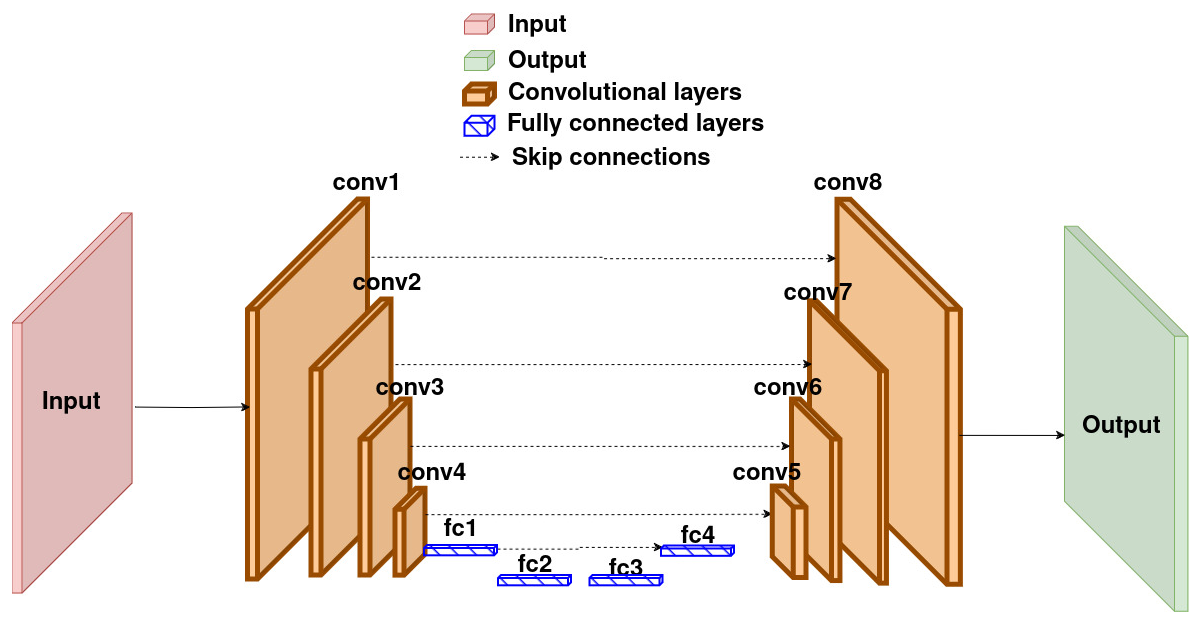
Figure 1 Architecture of a UNet with both convolutional and feed-forward layers. Here, the encoder and decoder are symmetrical.

GANs (Goodfellow et al., 2020) are a type of NN that actually consist of two networks. One is called the generator, and the other is the discriminator. The role of the discriminator is to distinguish between real data and data generated by the generator. The purpose of the generator is to produce output close enough to the real data that the discriminator labels them as real. These two networks learn competitively: the higher the loss of the generator, the lower the loss of the discriminator, and inversely. This allows such models to show interesting performances in the context of semi-supervised learning. They are also highly efficient for image-to-image translation tasks. The learning process of the type of GAN that will be used in this paper is described in Dabrowski et al. (2023), in Fig. 1 of that article.

4.2 Relevant deep learning models and architectures

Different types of models are implemented, trained and tested on our data. We use as the baseline for comparison the random forest algorithm (a machine learning algorithm), a polynomial interpolation method (of degree 3), and a kriging algorithm as described in Sect. 4.1.

Two deep convolutional neural network architectures, UNets and BC-GANs (Dabrowski et al., 2023), are the basic components of the models we propose in this paper. The first one is a purely supervised UNet and the second one a semi-supervised BC-GAN as described in Sect. 2. The architecture of the generator of these BC-GANs will each time correspond to the architecture of the corresponding purely supervised UNet. As for the architecture of the discriminators, they are described in Appendix B.

These models allow one to leverage sparse ground truth when complete ones are unavailable, which increases performance (compared to classical GANs) in the context of semi-supervised learning.

Indeed, we do not have access to complete ground truths for the whole training set. For a part of it, we only have access to sparse ground truths. The authors of Dabrowski et al. (2023) were mainly interested in how these sparse ground truths and the information they represent could be leveraged in order to ease the training and obtain better results. They proposed a method to leverage those sparse ground truths based on the literature around physics-informed networks that implied seeing those sparse ground truths as boundary conditions (BCs), hence giving it the name BC-informed GAN. The authors of Dabrowski et al. (2023) illustrated this method in Fig. 2 of their article. It includes the design of an additional loss function in order to train the model to respect the BCs. This essentially allows for localised supervision.

4.3 Information fusion strategies

All our models have in common that they use as input one or several variables to produce the same type of output. It is therefore necessary to merge these variables together during this process. This also ensures the production of the output makes use of all these pieces of information.

Fusion strategies are therefore an important aspect of the architecture definition, and eventually the performance, of the model. They represent different methods that can be applied to leverage several sources of data (several inputs) within the same NN. They can be applied on models such as UNets as well as GANs. There are three main different fusion strategies according to Mangai et al. (2010), namely, data fusion, feature fusion and decision fusion. Section 4.3.1, 4.3.2 and 4.3.3 describe (respectively) each of these approaches and the way we use them.

4.3.1 Data fusion (channel concatenation)

The general idea behind this strategy is to use several pieces of raw data to build a new, more complete and useful, piece of raw data.

As our data consist of images, the simplest way to do data fusion is to realise channel concatenation: in other words, to use our different inputs as if they were different channels of one single image. For this reason, this method is also called channel concatenation throughout this paper. This approach if the most straightforward of the three.

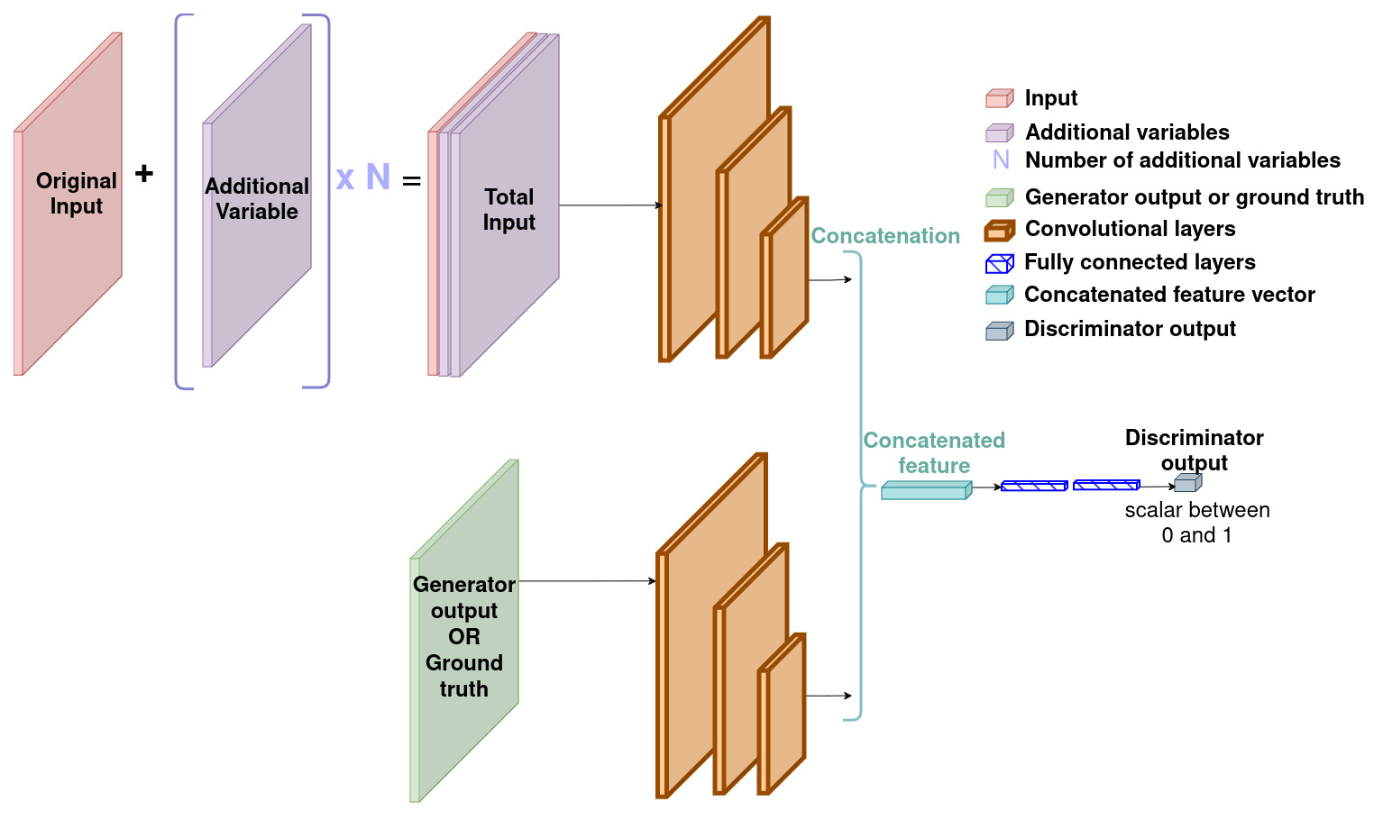
In terms of architecture of our neural networks, this simply implies using more convolutional filters. The UNet's architecture with data fusion is illustrated by Fig. 2. GAN's discriminator's architecture with data fusion is illustrated by Fig. B1 in Appendix B.

In terms of interpretation, this architecture relies on the local (rather than global) relationships between the different quantities used as input. We believe this architecture to work better if local patterns in one input image correspond to local patterns in other input images.

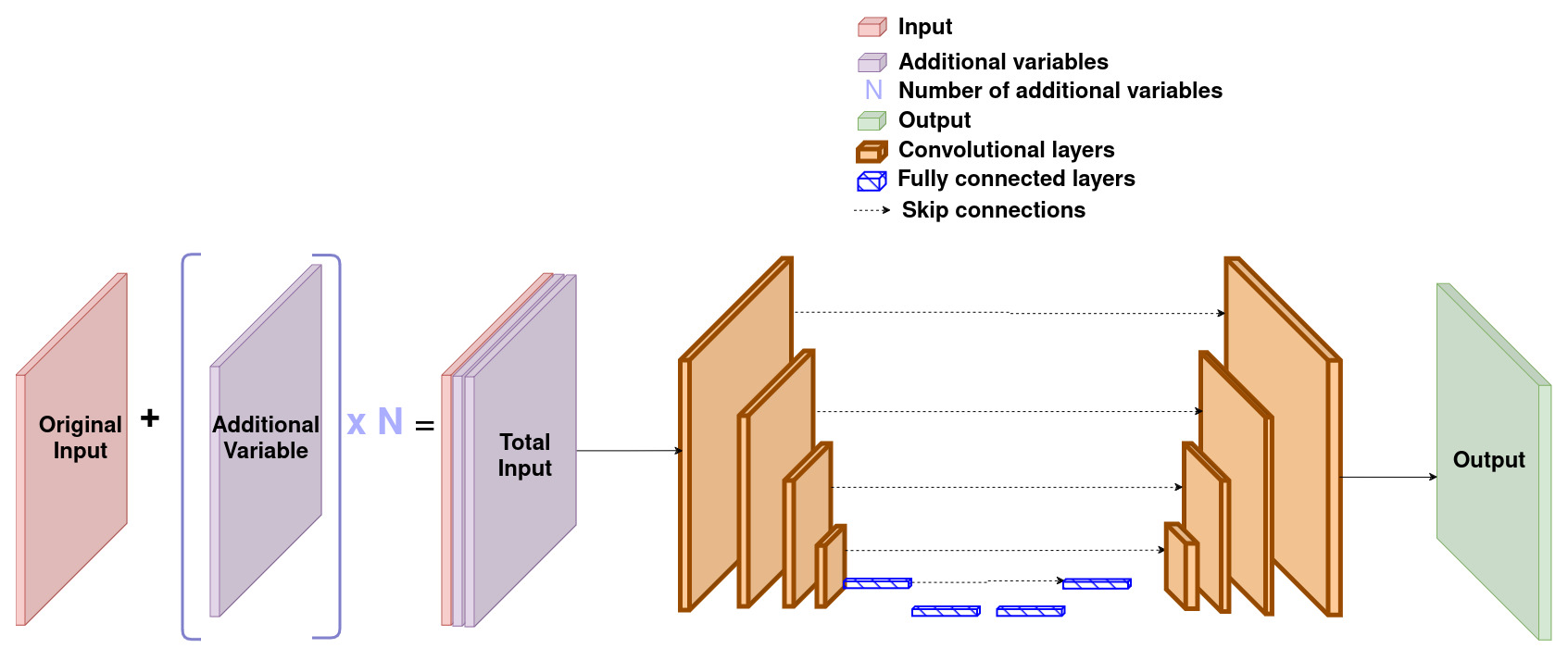
Figure 2 Architecture of the UNet with the data fusion approach. Also corresponds to the architecture of GAN's generator.

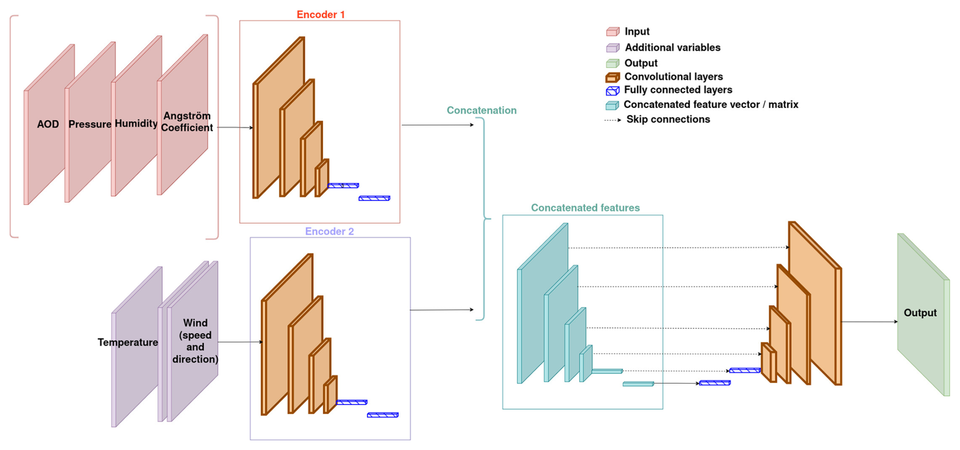
4.3.2 Feature fusion

One of the most common architectures in neural networks for computer vision tasks is the encoder–decoder. The general idea is that the encoder generates what is called a feature. This feature is usually a vector but can technically also be a matrix (although the idea is for it to be of smaller dimensions than the input). It is supposed to contain all the relevant information from the input with regard to the task at hand. In other words, it describes the input well enough so that only this feature is needed for the task. During the next step, the decoder uses the feature as input and produces the output.

Feature fusion methods are often applied to computer vision tasks, for example, when dealing with complex hyperspectral images (Song et al., 2018). The idea behind them is to obtain a feature for each input and use them to obtain one super-feature (for example by simply concatenating the various features). According to the authors of Sun et al. (2005), two interesting ways to fuse feature vectors are the serial feature fusion (based on an union vector) and the parallel feature fusion (based on a complex vector), although the same authors actually propose a new method based on canonical correlation analysis (CCA).

This unique feature is then used by the decoder to produce the output. In terms of architecture, this implies having as many encoders as inputs, but only one decoder (since there is only one output). The UNet's architecture with feature fusion is illustrated by Fig. 3.

The UNet architecture is a specific type of encoder–decoder, in which a specific type of connection, called skip connection, can be found. It is also often symmetric (in the sense that the decoder's layers mirror the encoder's one). After each layer in the encoder, the obtained feature is sent to the corresponding layer in the decoder. This allows for the decoder to have access to several features rather than simply the smallest one.

Implementing feature fusion with a UNet is therefore non-trivial: among all the features obtained for each input, which ones should be sent to the decoder through skip connections? We choose to apply what we call multiple-feature fusion. The principles of feature fusion are applied to a feature of each and every scale, and those merged features are sent to the corresponding layer of the decoder through skip connections.

In terms of interpretation, this architecture relies on the global relationships between the inputs. As obtaining features relies on dimension reduction, those features represent the input in a more global way and do not necessarily represent local patterns. The smaller the scale of these features (and the deeper their corresponding layers are), the truer it is. This architecture relies on the idea that each of the input images contains a global, non-localised piece of information that can be useful in order to estimate the aerosol concentration. Again, the global or non-localised aspect of each of the features actually depends on its scale or depth in the network.

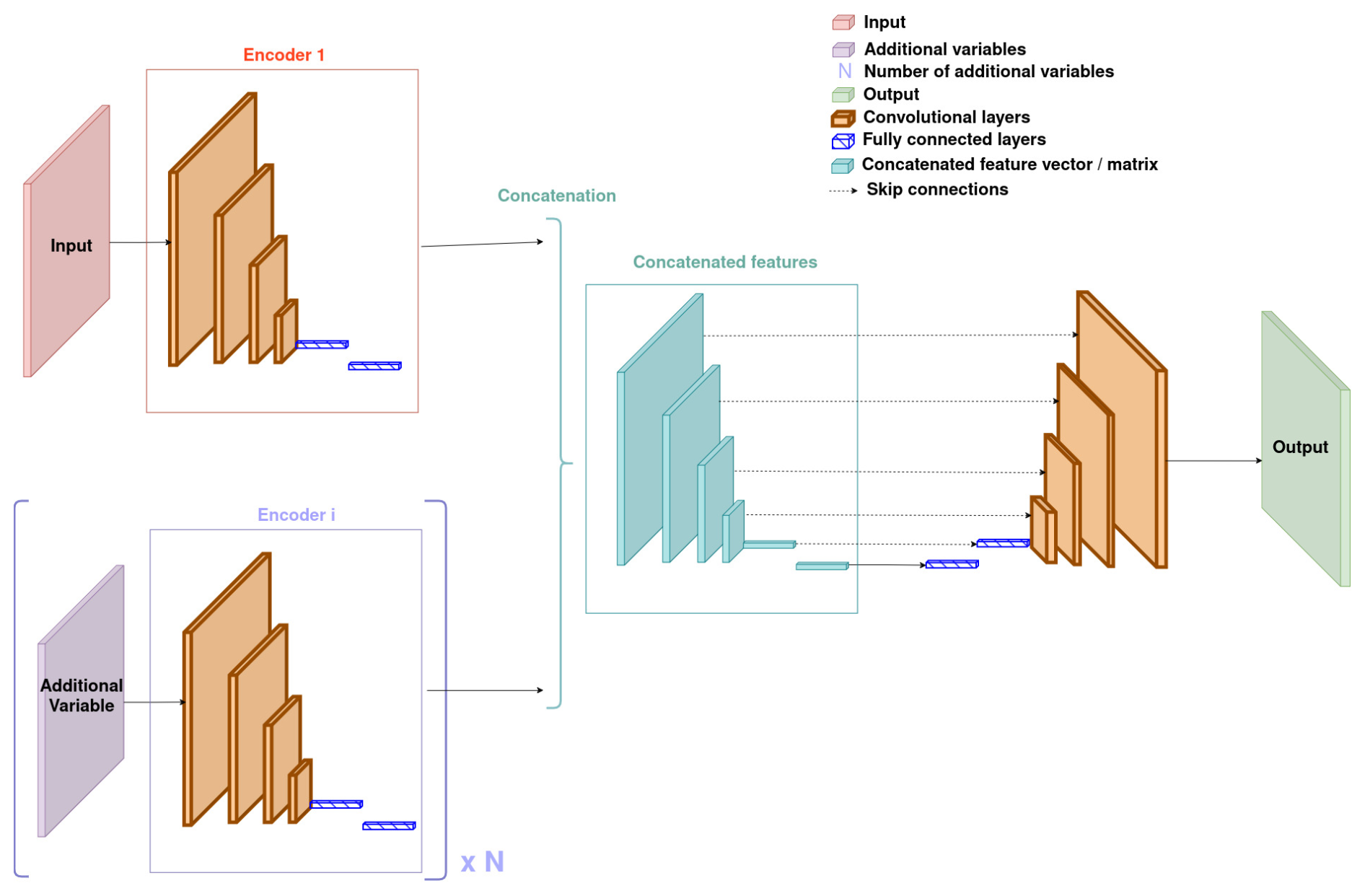
Figure 3 Architecture of the UNet with the feature fusion approach. It also corresponds to the architecture of GAN's generator.

GAN's discriminator's architecture with feature fusion is illustrated by Fig. B2 in Appendix B.

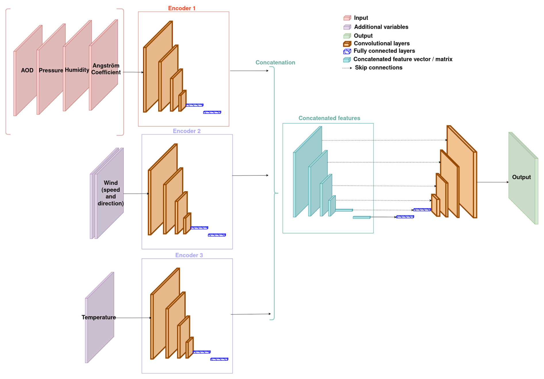
4.3.3 Decision fusion

The idea behind decision fusion is to use a separate model for each input, obtain an output for each of them, and then merge those outputs together to obtain a final decision, which is supposedly better. In classification tasks, decisions represent the predicted class. In regression tasks, like the one considered in this paper, they represent the estimated quantity. Losses are computed using the final output. The backpropagation process takes place through the entire model (and the smaller models that compose it).

There exist several ways to fuse decisions, such as the linear or log opinion pool (corresponding respectively to a weighted sum or product) (Sinha et al., 2008). Voting algorithms can even be used for classification tasks (Sinha et al., 2008). In this article, a linear opinion pool approach is chosen: we apply a weighted mean of all the outputs to obtain the final one. The weights are learnable parameters, which allows the model to learn which outputs are most relevant.

This principle relies on the idea that each of the inputs can individually be used to produce an estimation of the aerosol concentration but that these estimation may be flawed and that the best estimation can be obtained through a combination (here a weighted mean) of these flawed estimations. In other words, it is possible to correct the estimation produced with an input using the estimation produced with another input. Since the model can learn which inputs are the most relevant to produce the desired output, we expect this approach to provide the best inference when all inputs are used.

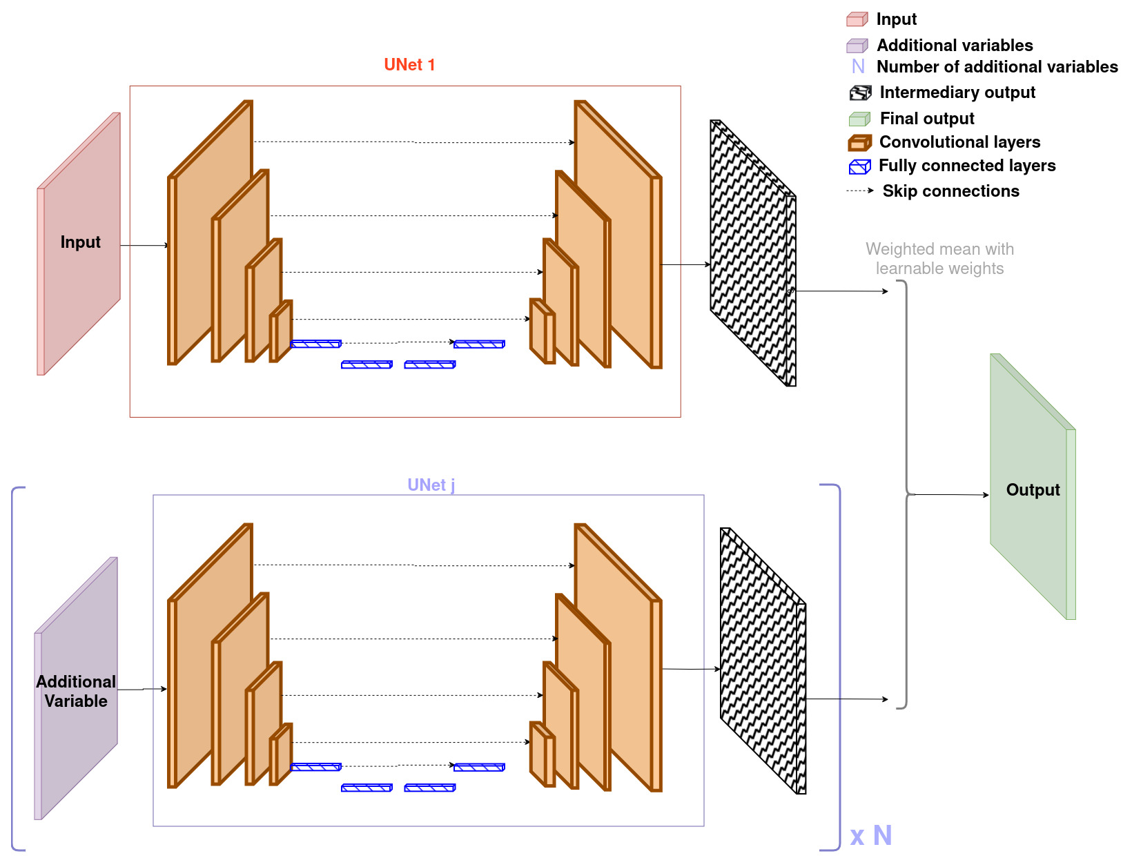
Figure 4 Architecture of the UNet with the decision fusion approach. It also corresponds to the architecture of GAN's generator.

The architecture of GAN's discriminator with decision fusion is, in principle, very similar to the architecture of our UNet with decision fusion. The main difference is the type of output, as the discriminator outputs a single scalar for each iteration, while the UNet outputs images. It is illustrated by Fig. B3 in Appendix B.

4.3.4 Hybrid fusion models

The physical nature of PM_2.5 predictors obviously has an impact on the non-linear function linking AOD and PM_2.5. While AOD is directly linked to total column aerosol concentration at a given location, surface pressure can indirectly be linked to PM_2.5 through accumulation in the atmospheric boundary layer under stable conditions, while wind speed can influence PM_2.5 concentration over a longer range in space and time. Therefore we can distinguish “state” variables that can directly link PM_2.5 to AOD through an integral expression over the atmospheric column and “indirect predictors” that act on PM_2.5 concentrations over different space and timescales. In our current analysis, the wind variables (speed and direction) stand out as they describe the atmosphere dynamics, while the AOD and Ångström exponent are clearly state variables regarding the inference of PM_2.5 concentration. Humidity, pressure and temperature variables can be considered primarily state variables as they strongly impact the particle size distribution through aerosol hygroscopicity but can also indirectly influence near-surface PM_2.5 concentrations by favouring accumulation under stable atmospheric conditions or, on the contrary, by the removal of atmospheric particles through dry deposition or wet scavenging.

The performance of networks and their robustness to noise are known to be impacted by their architecture, and network performances can be improved upon state-of-the-art (SOTA) when the network is well aligned with the target function (Li et al., 2021). We hypothesise here that for atmospheric applications, the optimal alignment of network architecture with the target function may depend on the nature of variables used as input and on the fusion strategy used for merging information carried by those variables. Through this hypothesis, we ask whether there is an advantage in applying different fusion strategies for different types of input variables.

Based on this insight, we propose two hybrid models using different fusion strategies depending on the variable considered. The idea is to use data fusion (channel concatenation) for the AOD and all other input variables, except for the wind and temperature, for which feature fusion is used. Figures 5 and 6 describe these two models more precisely. Section 6.5 shows and discusses the results obtained by these models.

Figure 5 The first proposed hybrid model using both data fusion and feature fusion.

Figure 6 The second proposed hybrid model using both data fusion and feature fusion.

5 Methodology

In order to find the best way to handle our variety of input quantities, we propose to study the three main fusion approaches described in Sect. 4.3. Each fusion method is experimented on using two types of models: a purely supervised UNet and a BC-GAN using sparse measurements of the aerosol concentration at ground level as boundary conditions. Experiments on the hybrid approaches proposed in Sect. 4.3 are realised as well.

The goal is also to understand which input quantities have the most important impact on our results, in other words, which additional variables actually help our models to better predict PM_2.5 at surface level. This is why, for each distinct model architecture, experiments are realised with different combinations of additional variable to study their impact on the results.

5.1 Learning and validation protocol

Experiments are conducted on CAMS and ALADIN datasets. AOD is systematically used as input in all our experiments. In addition, six other variables are also considered (wind speed and direction, relative humidity, atmospheric pressure, temperature, and Ångström exponent) in order to evaluate their impact on the results. It is important to specify that the wind speed and direction are always used jointly to describe the wind state variable. With this rule in mind, experiments are performed with all possible combinations of these six variables (including using none of them and all of them). The AOD is also used in all cases.

For both CAMS and ALADIN datasets, we always consider the same type of scenario, shown by Fig. 7. In this scenario, we have access to a dataset with complete ground truths, corresponding to a period of 11 months. We also have access to a second dataset with sparse ground truths, which can therefore only be used in the context of semi-supervised (as opposed to purely supervised) learning, corresponding to a period of 1 month. These sparse ground truths will be used as boundary conditions as stated in Sect. 2. They contain a number of pixels corresponding to 5 % of the pixels available in complete ground truths.

For the CAMS dataset, one sample is generated every 3 h. Samples take the form of matrices of size 241×480. Depending on the chosen number of input modalities, each model input can be composed of one to seven of these matrices. The training set therefore contains 2680 of these inputs, the sparse training set (with sparse ground truths) 240 inputs and the test set 2920 inputs.

For the ALADIN datasets, one sample is generated every hour. The size of the matrices is 405×613. Again, depending on the chosen number of input variables, each model input can be composed of one to seven of these matrices. The training set therefore contains 8040 of these inputs and the sparse training set (with sparse ground truths) 720 inputs. For the test set, we only use one image for every 3 h so that it contains as many samples as the CAMS test set. Therefore it also contains 2920 inputs.

An exhaustive study on our two models (UNets and GANs), three fusion strategies and six input variables (and all possible combinations of these) is conducted on the CAMS dataset. This corresponds to 192 different experiments. Only experiments that lead to the best performances on the CAMS dataset are conducted on the ALADIN dataset. The aim is to provide an insight into the impact of the characteristics of each dataset on the results, as shown in Sect. 6.2.

Then, experiments are realised on the hybrid approaches, but only on UNet models, and always with all six additional input variables. These experiments are realised on both datasets as well.

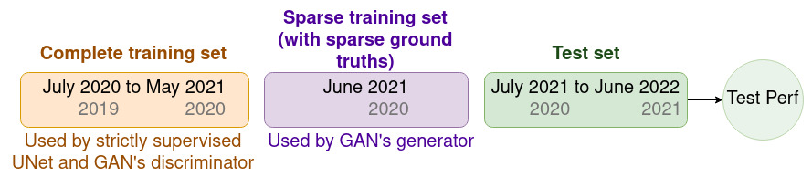
Figure 7 Representation of the datasets used for our experiments. The text in grey specifies the corresponding periods of time for the datasets built with the data from the ALADIN model instead of the CAMS model.

5.2 Data pre-processing

All values of AOD inferior to 0.005 can be considered noise. They are therefore set to 0 before being used, be it for training or prediction.

In order to speed up the convergence of the models, we equalise the PM_2.5 and AOD distributions by applying the function ln (1+x) to those values. The inverse function exp (x)−1 is then simply applied to inferred outputs in order to obtain actual concentration values (in µg m⁻³) and ease the interpretation of our results. In our context, polluted regions (with high aerosol concentration values) are our areas of main interest. Therefore, filtering very low aerosol concentration values in our ground truths and predictions allows us to better evaluate the model performance in these areas. Specifically, values inferior to 1 µg m⁻³ are set to 0 µgm⁻³. This is done before computation of the evaluation metrics.

These previous pre-processing protocols are based on the protocols proposed by Dabrowski et al. (2023).

The data give us access to values of both eastward and northward wind speeds. Instead of using them as such, we apply the transformation described by Eq. (1) to instead obtain two different matrices. In this equation, U and V respectively represent the eastward and northward wind speeds. The first one contains values of the wind speed norm (regardless of direction) and the second one values of the direction (in degrees) of the wind. Each time wind values are used in an experiment, both of these matrices are used.

$$\begin{array}{}\text{(1)}& \begin{array}{rl}\mathbf{norm}=& \sqrt{U^{\mathrm{2}}+V^{\mathrm{2}}}\\ \mathbf{direction}=& \arctan \left({\displaystyle \frac{\mathbf{V}}{\mathbf{U}}}\right).\left({\displaystyle \frac{\mathrm{180}}{\mathit{\pi }}}\right)\end{array}\end{array}$$

Our data do not originally contain values of the Ångström exponent, but it is easily possible to compute them using values from the AOD measured at two different wavelengths and Eq. (2). In this equation, λ₁ represents the wavelength of the original AOD, which is 550 nm, and λ₂ is the wavelength of the second AOD, used simply to compute the Ångström exponent. When using data from the CAMS model, this second wavelength is 865 nm, while with the ALADIN model, it is 1000 nm.

$$\begin{array}{}\text{(2)}& \mathbf{angstrom}({\mathit{\lambda }}_{\mathrm{1}},{\mathit{\lambda }}_{\mathrm{2}})=-{\displaystyle \frac{\ln \left(\frac{\mathbf{AOD}\left({\mathit{\lambda }}_{\mathrm{2}}\right)}{\mathbf{AOD}\left({\mathit{\lambda }}_{\mathrm{1}}\right)}\right)}{\ln \left(\frac{{\mathit{\lambda }}_{\mathrm{2}}}{{\mathit{\lambda }}_{\mathrm{1}}}\right)}}\end{array}$$

Pressure values are converted from pascals to atmospheres, and temperature values from kelvins to Celsius degrees.

5.3 Metrics and losses

During training, depending on the type of model, different losses can be used. For our GANs, the adverse loss is used (to train both the generator and the discriminator), as well as the boundary condition loss (which is essentially a localised mean squared error (MSE), as stated in Sect. 2). This last loss is described by Eq. (3), where y is the ground truth, $\widehat{\mathbf{y}}$ represents the output of the model, and BC is a matrix containing 1 at the location of known values of y and 0 elsewhere.

$$\begin{array}{}\text{(3)}& \mathrm{BCloss}(\mathbf{BC},\widehat{\mathbf{y}},\mathbf{y})=\mathrm{MSE}(\mathbf{BC}\cdot \widehat{\mathbf{y}},\mathbf{BC}\cdot \mathbf{y})\end{array}$$

For our supervised UNets, we use the MSE loss function as well as the feature similarity (FSIM) (Zhang et al., 2011), which is also used as a metric and described in this section.

Four metrics are used to evaluate the models during testing: the mean absolute error (MAE), the mean bias error (MBE) and the quantised error (QE), as proposed by Dabrowski et al. (2023), as well as a metric proposed by Zhang et al. (2011) called the FSIM. The MAE and MBE are expressed in µg m⁻³ (the unit of aerosol concentration) and in percentages (for their relative versions).

In the following equations, y represents the ground truth, y_i its elements and $\stackrel{\mathrm{‾}}{y}$ its average. $\widehat{\mathbf{y}}$ is the output of the model and ${\widehat{y}}_i$ its elements. The number of elements in either matrix is N.

• Mean absolute error (MAE). It is the most widely used of these metrics; it represents the error of the models in a general sense (Wang and Lu, 2018). It is described by Eq. (4), in which y is the ground truth, $\widehat{\mathbf{y}}$ represents the output of the model, and N represents the number of pixels in y.

  $$\begin{array}{}\text{(4)}& \mathrm{MAE}(\widehat{\mathbf{y}},\mathbf{y})=\left|{\displaystyle \frac{\mathbf{y}-\widehat{\mathbf{y}}}{N}}\right|\end{array}$$

  Equation (5) describes the way the rMAE is computed from the MAE using $\stackrel{\mathrm{‾}}{y}$, the average of the ground truth y.

  $$\begin{array}{}\text{(5)}& \mathrm{rMAE}(\widehat{\mathbf{y}},\mathbf{y})={\displaystyle \frac{\mathrm{MAE}(\widehat{\mathbf{y}},\mathbf{y})}{\stackrel{\mathrm{‾}}{y}}}\end{array}$$

• Mean bias error (MBE). It represents the model's tendency to overestimate or underestimate the values to predict. A model with poor performance can, however, still have a low bias as it is not the only aspect of its performance. This error can sometimes be used to correct the bias of the model. It is described by Eq. (6), which uses the same notation as Eq. (4).

  $$\begin{array}{}\text{(6)}& \mathrm{MBE}(\widehat{\mathbf{y}},\mathbf{y})={\displaystyle \frac{\mathbf{y}-\widehat{\mathbf{y}}}{N}}\end{array}$$

  Equation (7) describes the way the rMBE is computed from the MBE using $\stackrel{\mathrm{‾}}{y}$, the average of the ground truth y.

  $$\begin{array}{}\text{(7)}& \mathrm{rMBE}(\widehat{\mathbf{y}},\mathbf{y})={\displaystyle \frac{\mathrm{MBE}(\widehat{\mathbf{y}},\mathbf{y})}{\stackrel{\mathrm{‾}}{y}}}\end{array}$$

• Quantised error (QE). This metric is used to quantise the prediction as well as the ground truth before comparing them. The quartiles of the ground truth values distribution (q1, q2, q3 and q4) are used to define four classes for this quantisation process, which is described by Eq. (8). In this same equation, M_i,j represents a pixel of coordinates (i,j) from the unquantised matrix M. C_i,j represents the pixel with these same coordinates in the corresponding quantised matrix C.

  $$\begin{array}{}\text{(8)}& C_{i,j}=\left\{\begin{array}{ll}\mathrm{0}& \text{if }{M}_{i,j}\le q\mathrm{1}\\ \mathrm{1}& \text{if }{M}_{i,j}\in (q\mathrm{1},q\mathrm{2}]\\ \mathrm{2}& \text{if }{M}_{i,j}\in (q\mathrm{2},q\mathrm{3}]\\ \mathrm{3}& \text{if }{M}_{i,j}>q\mathrm{3}\end{array}\right.\end{array}$$

  This process allows us to obtain a quantised ground truth C_gt and a quantised prediction C_pred. The quantised error is computed from these matrices following Eq. (9). N represents the number of pixels in matrix C_gt in this equation.

  $$\begin{array}{}\text{(9)}& \mathrm{QE}={\displaystyle \frac{|{\mathbf{C}}_{\mathrm{gt}}-{\mathbf{C}}_{\mathrm{pred}}|}{N}}\end{array}$$

  This type of metric is usually better suited for classification or segmentation tasks. However, the air quality is often represented as indexed values and involves thresholds corresponding to different levels of health hazards (or policy alerts): this metric is therefore more closely related to this representation. It is also more sensitive than the MAE to very localised errors. It is, on the other hand, less suited to represent tendencies to generally overestimate or underestimate the values to predict than the MBE.

• Feature similarity index (FSIM). This metric has been proposed by the authors of Zhang et al. (2011) as an image quality assessment metric. It relies on the concepts of phase congruency and gradient magnitude (in the sense of image gradients). The phase congruency is also used to weigh the contribution of each pixel to the similarity between two images. This leads to a significant weight being given to edges, shapes and other structures in the images.

5.4 Scores

As a great number of experiments were realised during this work, we can not easily compare them all in a table. We decide to present an overview of these results through charts and to select a few experiments to compare in a table. Since a lot of different metrics are used, a protocol is needed to select the experiences to compare. Three different scores, computed from the previously described metrics, are used. This allows us to select experiments that lead to good overall results rather than experiments that performed well on one metric and poorly on all others, for example. These scores are exclusively used for this selection process and do not intervene further when interpreting and analysing our results. For this reason, and to avoid overloading our result tables, the score values are not presented in these same result tables.

• Total score. This score is computed using all of our metrics at the same time, including the inference time. It follows Eq. (10). rMAE and rMBE represent the relative counterparts of MAE and MBE and are expressed in percentages instead of in µg m⁻³. Regarding the inference time, the threshold of 0.05 s is used as it is the maximum inference time among our experiences with our deep learning models.

  $$\begin{array}{}\text{(10)}& \mathrm{\text{Total score}}={\displaystyle \frac{\begin{array}{c}\frac{\mathrm{0.05}\text{s-Inference time}}{\mathrm{0.05}\mathrm{s}}+(\mathrm{1}-\mathrm{rMAE})\\ +\frac{\mathrm{3}-\mathrm{QE}}{\mathrm{3}}+(\mathrm{1}-\mathrm{rMBE})+(\mathrm{1}-\mathrm{FSIM})\end{array}}{\mathrm{5}}}\end{array}$$

• Timeless score. This score is very similar to the first one but does not include the inference time metric. This allows for the identification of the best-performing models for a situation in which the inference time is not a predominant factor. It follows Eq. (11).

  $$\begin{array}{}\text{(11)}& \text{Timeless score}={\displaystyle \frac{\begin{array}{c}(\mathrm{1}-\text{rMAE})+\frac{\mathrm{3}-\mathrm{QE}}{\mathrm{3}}\\ +(\mathrm{1}-\mathrm{rMBE})+(\mathrm{1}-\mathrm{FSIM})\end{array}}{\mathrm{4}}}\end{array}$$

• Reduced score. This score is computed using only rMAE and FSIM. These two metrics are the most relevant ones in the computer vision domain. This score therefore allows for a comparison of the models and experiments from this point of view only. It also does not make use of the inference time. It follows Eq. (12).

  $$\begin{array}{}\text{(12)}& \text{Reduced score}={\displaystyle \frac{(\mathrm{1}-\mathrm{rMAE})+(\mathrm{1}-\mathrm{FSIM})}{\mathrm{2}}}\end{array}$$

5.5 Methodology and data summary

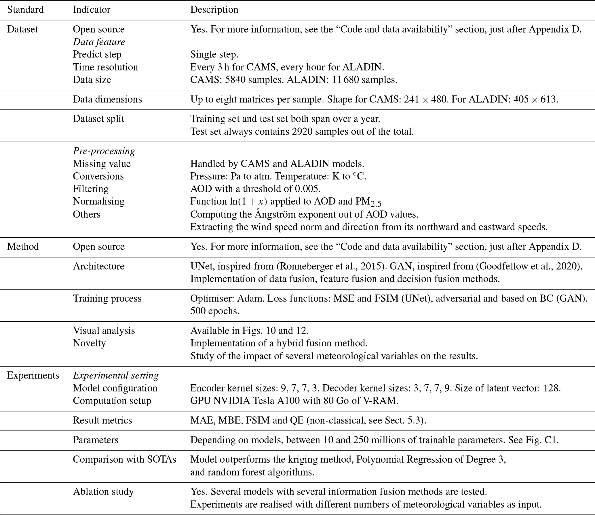
In order to ease the comparison of this work to other models using a scaling approach for inference of PM_2.5 from AOD, we provide hereafter in Table 1 a summary of our methodology as well as some characteristics of the dataset and methods used in this paper. It follows the standard proposed by the authors of Zhou et al. (2024).

(Ronneberger et al., 2015)(Goodfellow et al., 2020)

Table 1 Characteristics of the dataset, method and experiments used in this paper in the standard proposed by the authors of Zhou et al. (2024). Indicators in italic represent subgroups of indicators belonging to the standard on the left.

6 Results

We start with a general overview of our results. The next step is to identify the best-performing and most interesting results and models among the experiments realised on the CAMS dataset. This allows us to reproduce these experiments on the ALADIN dataset in order to compare the results and better understand the impact of the characteristics of these datasets (namely, spatial domain and resolution) on the results.

6.1 Overview

We choose to summarise our results in the form of radar charts, with five metrics represented on these charts: the inference time t, rMAE, QE, rMBE and FSIM. The values of these metrics were normalised the same way they are when used to compute our scores, which allows us to represent them on the same scale. High values of these normalised versions of our metrics represent high performance. Lines made up of cyan dots represent both the maximum and minimum performances for each metric, and are linked by a light cyan area that gives an overview of the performance range on each radar graph. Blue dashes and dashed–dotted purple lines represent respectively the median and average performance for each metric among all results presented on this radar graph. Out of these same results, the experiments that lead to the obtention of the best total score are represented with a plain red line on the graph. The relative values (in percentages) of each metric for these experiments (the ones leading to the best score) are also systematically represented by yellow boxes on the graph.

Figure 8 gives an overview of the performance of each couple model-fusion strategy. It shows that, on average, models using decision fusion have the longest inference time, while models using data fusion are the fastest, and those using feature fusion are in the middle. This is expected as it correlates with the number of parameters of each model, as illustrated by Fig. C1.

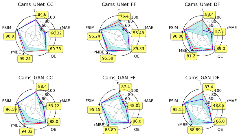
Figure 8 Overview of each model – fusion strategy couple. Regarding the fusion type, CC stands for channel concatenation or data fusion, FF stands for feature fusion, and DF stands for decision fusion. Cyan dots: maximum and minimum, with a cyan area in between. Blue dashes: median. Dashed–dotted purple lines: average. Solid red line: best total score (corresponds to annotated values).

It also shows that GANs seem to generally suffer from poorer rMAE and rMBE scores than UNets. Our interpretation is that the proportion of the training set reserved for strictly supervised training is important enough for purely supervised methods to perform well. The appeal of GANs lies in their ability to realise semi-supervised training. In our case, it also corresponds to their ability to make use of the portion of our dataset that only contains sparse ground truths. This portion is small, which therefore makes the appeal of GANs (and arguably semi-supervised methods) limited in this case. In comparison, the authors of Dabrowski et al. (2023) show the efficiency of their GANs in a context where only half of the dataset contains complete ground truths. It is interesting to note that the FSIM and QE metrics do not seem to be affected by this in the same way or, at least, not as intensely.

Finally, the data fusion or channel concatenation (CC in the figure) strategy seems to be leading to more stable results than the other two fusion strategies. This may also be linked to the difference in model complexity, as shown in Appendix C.

Figure 9 shows the evolution of the performances of our UNet when we increase the number of input variables. It shows that, when increasing the number of input variables, the average inference time increases. This is expected, as Fig. C1 shows that the models grow in complexity with the number of input variables. Other metrics, and especially rMAE, show on average an increase in performance when adding more input variables. However, this increase in performance is not linear, and when deciding to add an input variable to a given experiment, we are not guaranteed to obtain better results. We can also note that, when comparing experiments with two additional input variables to those with three, we observe less stable rMBE values even though the number of experiments for these two categories is the same. Finally, these charts also show that, regardless of the fusion method used, experiments realised using all five input variables tend to produce the best results (apart from the point of view of the inference time).

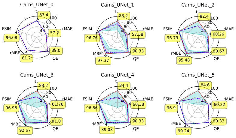
Figure 9 Overview of the evolution of our UNet's performances when increasing the number of input variables. The wind is counted as one variable even though it contains two channels (one for wind speed and a second one for direction). Cyan dots: maximum and minimum, with a cyan area in between. Blue dashes: median. Dashed–dotted purple line: average. Plain red line: best total score (corresponds to annotated values).

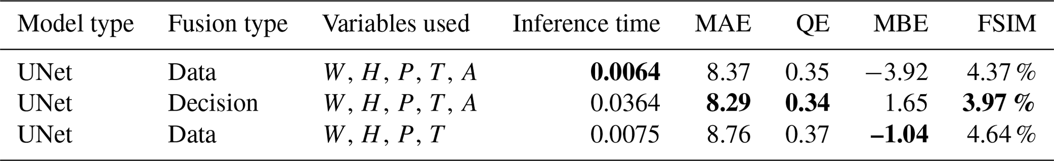
6.2 Best results on the CAMS dataset

Table 2 shows the best results according to each of the three scores. The first line is the result with the best total score, the second line is the best timeless score, and the third line is the best reduced score. Figure 10 shows the output of these models for one given sample.

Table 2 Best results on CAMS dataset. In the column Variables used, we put the initial of each used variable: W for wind, H for humidity, P for pressure, T for temperature and A for Ångström exponent. The AOD is always used as input. The column Fusion type contains data for data fusion, feature for feature fusion and decision for decision fusion. The first line is the result with the best total score, second line is the best timeless score, and third line is the best reduced score. For each metric column, the best value is formatted in bold.

This table shows that using more variables as input seems to generally lead to the best results, except for the Ångström exponent on the last line. It also shows that decision fusion methods suffer from larger inference times, especially compared to data fusion. These results lead to three main recommendations depending on the context and the desired performances. If the MBE (or bias) of the output is not an important factor, then the recommended model is a UNet using the data fusion strategy, as well all proposed input variables, except for the Ångström exponent. If the inference time is not an important factor, then the use of a UNet model with the decision fusion strategy and all proposed input variables is advised. Finally, a UNet with the data fusion strategy as well as all proposed variables gives the most balanced results.

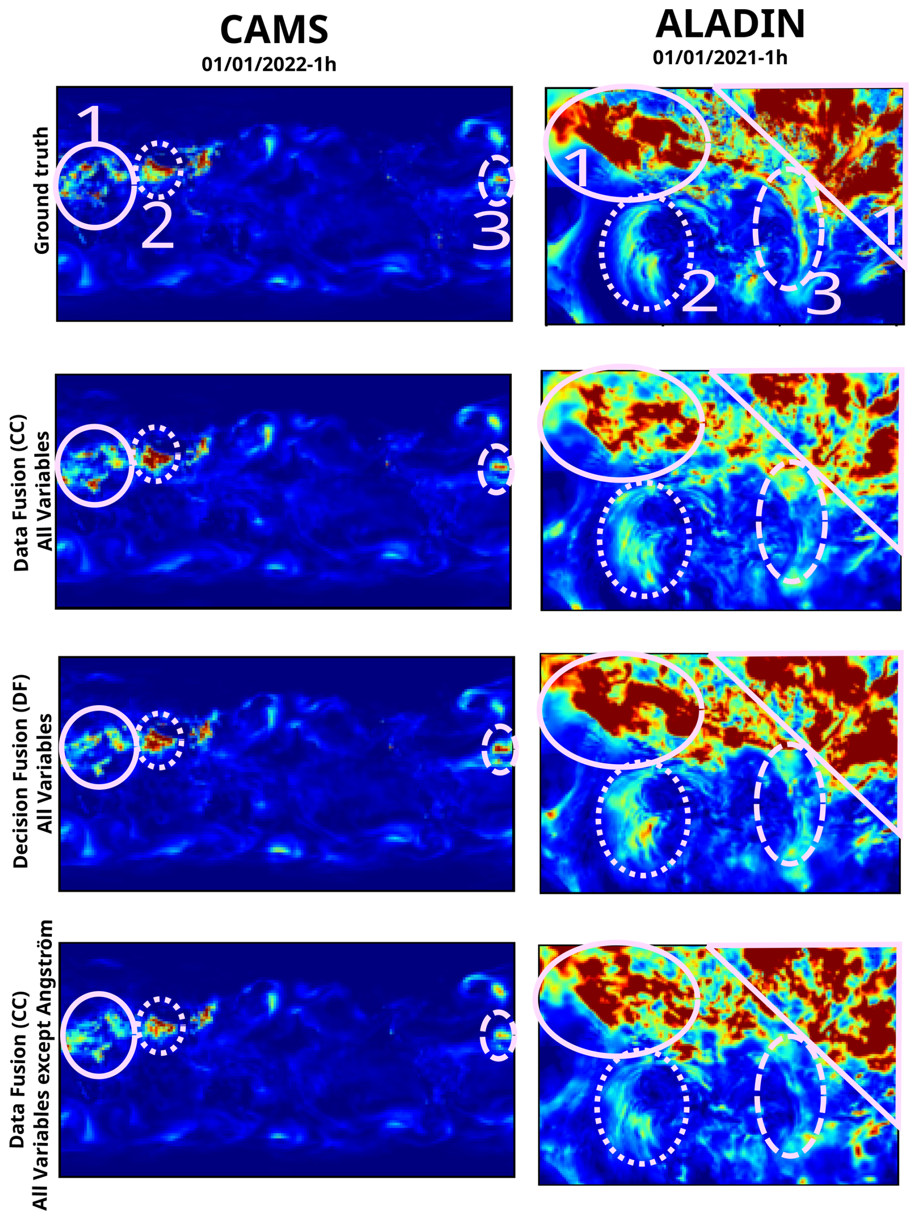
Figure 10 Outputs of the best models on both datasets for one given sample. The pink circles and numbers have been added afterwards to attract the reader's attention to some details of the image.

Looking at the left column Fig. 10 gives us a bit more insight into the results. On this sample, it seems that the model using data fusion and all variables except the Ångström exponent is the one providing the best prediction for area no. 2 in the image. Other models overestimate the aerosol concentration in this area. The fact that this model has the worst MBE and that it is negative could shows a tendency to underestimation. The observations made using this sample are coherent with this assumption. The model using data fusion and all variables, however, provides good estimations for these two areas. Finally, the model using decision fusion (and all variables) underestimates the concentration in area no. 1 and overestimates it in areas no. 2 and 3. This model has the best MBE but not the best MAE. Our hypothesis is that it overestimates certain areas and underestimates others, which by compensation leads to a small bias.

6.3 Comparison between the CAMS and ALADIN datasets

Table 3 shows the results obtained for the same models as in Sect. 6.2 but on the ALADIN dataset, and the right column of Fig. 10 shows their outputs for one given sample.

Table 3 Results on ALADIN dataset. In the column Variables used, we put the initial of each used variable: W for wind, H for humidity, P for pressure, T for temperature and A for Ångström exponent. The AOD is always used as input. The column Fusion type contains data for data fusion, feature for feature fusion and decision for decision fusion. For each metric column, the best value is formatted in bold.

The table shows an important difference between the results obtained on the CAMS and the ALADIN datasets. However, even though the same metrics are used, these sets of results are not easily comparable to each other as they are obtained on different data. Indeed, the ALADIN dataset contains images of much higher resolution than the CAMS dataset; these images do not represent the same geographical domain (Europe for ALADIN, the world for CAMS), and these datasets do not correspond to the same time period (July 2020 to June 2022 for CAMS, July 2019 to June 2021 for ALADIN). This explains why, in the CAMS dataset, the aerosol concentration values are between 0 and 34 425 µg m⁻³, with an average of 11.02 µg m⁻³, while in the ALADIN dataset, they are between 0 and 6774 µg m⁻³, with an average of 23.17 µg m⁻³.

Figure 10 also shows a difference between results using the CAMS and ALADIN datasets. The model using data fusion with all variables underestimates the aerosol concentration in areas no. 1 and 3, which is consistent with the fact that this model has the lowest MBE out of the three. The model using data fusion and all variables except the Ångström exponent also underestimates concentration in these areas but less so. This is coherent with the fact that of all three models, this one has the second-lowest MBE. The model using decision fusion does not underestimate concentration in areas no. 1, underestimates the concentration in area no. 3 as all other models, and overestimates the concentration in area no. 2. It is also the model with the highest MBE and the best MAE out of all three.

Comparison between results on our two datasets does remain interesting as the best-performing methods on the CAMS dataset do not seem to correspond to the best-performing ones on the ALADIN dataset. For example, let us look at the results from the table obtained with the data fusion strategy. One of these results is obtained while using all available variables as input, and the other is obtained using all variables except the Ångström exponent. Based solely on these two results, on the CAMS dataset, it would seem that using the Ångström exponent as part of the input variables leads to a smaller MBE, but we obtain higher values for all other metrics (except the inference time). On the ALADIN dataset the same situation and decision (of using the Ångström exponent) seem to lead to opposite results (higher MBE, smaller rest of the metrics). This also shows that the impact of the use of one specific input variable on the results of our models can not easily be interpreted. This is due to the interaction between the input variables themselves and the very nature of the neural networks, which are often described (with reason) as black boxes.

6.4 Interpretation of the impact of the Ångström exponent

Let us look at Fig. 11 to try and understand the impact of using the Ångström exponent on our results on the CAMS dataset. This figure shows that the two metrics that are impacted the most by the use of the Ångström exponent are the MAE and the MBE (and their relative counterparts). Using the Ångström exponent seems to lead to a higher minimum value for the MAE. In other words, it helps to avoid our worst results (with respect to the MAE). The best MBE values are obtained when using the Ångström exponent. Using it therefore seems to lead to a lower bias.

Once again, these observations are valid for the CAMS dataset and for the chosen periods. We can not make a general conclusion on the use of the Ångström exponent as an input variable based on these observations alone. In particular, these observations are consistent with the results shown in Table 2 (obtained with the CAMS dataset) but not with those in Table 3 (obtained with the ALADIN dataset). This shows that our observations (about the Ångström exponent) on the CAMS dataset can not automatically be assumed to be true for the ALADIN dataset too.

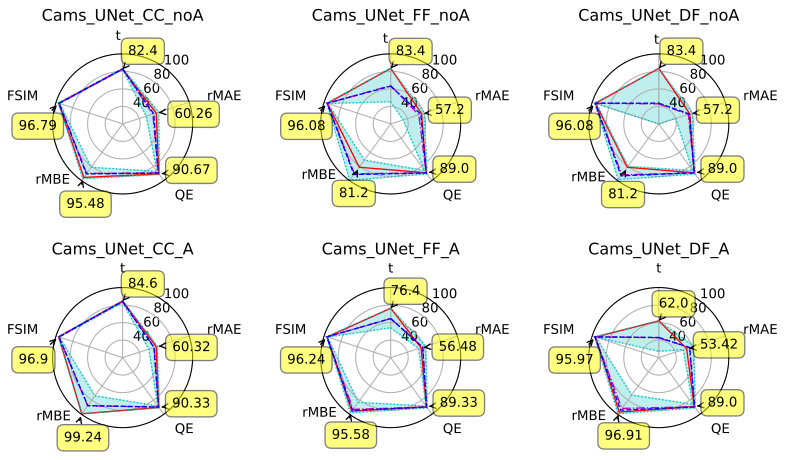
Figure 11 Overview of our experiments with (first line) and without (second line) the Ångström exponent as an input variable. Regarding the fusion type, CC stands for channel concatenation or data fusion, FF stands for feature fusion, and DF stands for decision fusion. Cyan dots: maximum and minimum, with a cyan area in between. Blue dashes: median. Dashed–dotted purple lines: average. Plain red line: best total score (corresponds to annotated values).

6.5 Results of hybrid fusion method

Tables 4 and 5 shows the results of the two hybrid models described in Sect. 4.3.4 on the CAMS and ALADIN datasets respectively. Figure 12 shows the outputs of these models on one given sample.

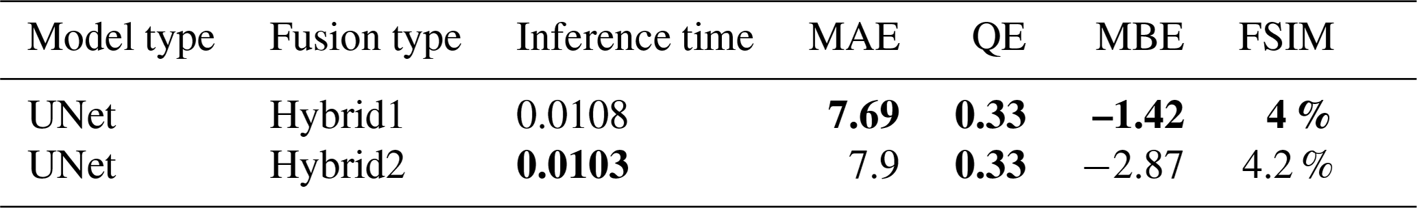
Table 4 Results of hybrid models on the CAMS dataset. The column Fusion type contains Hybrid1 for the model represented by Fig. 5 and Hybrid2 for the model represented by Fig. 6. For each metric column, the best value is formatted in bold.

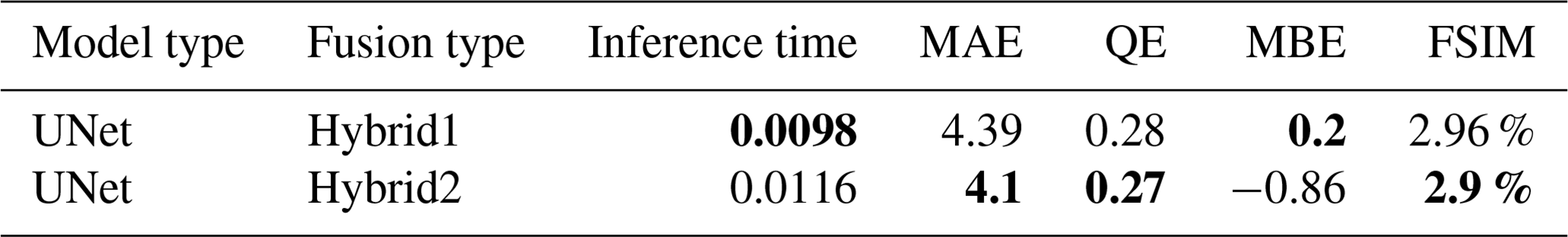
These results show that, from an artificial vision point of view, the second proposed hybrid model is better. However, the first model appears to be more balanced and is recommended in any situation where the MBE and inference time are important metrics.

These models, while showing satisfying performance, show poorer performances than some of the results presented in Table 2. Therefore, we do not recommend the use of these hybrid models with the CAMS dataset.

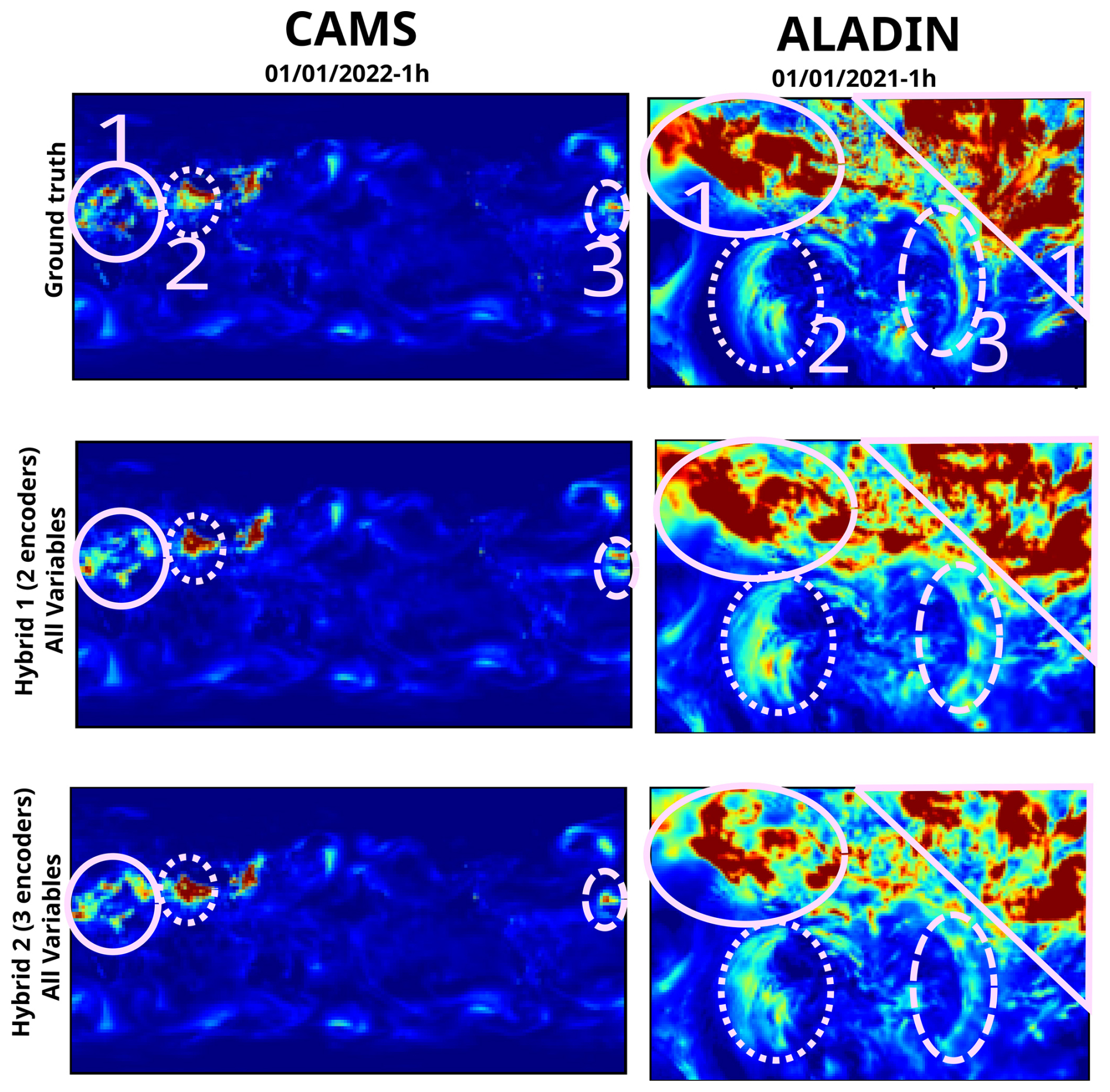
Figure 12 Outputs of hybrid models on both datasets for one given sample. The pink circles and numbers have been added afterwards to attract the reader's attention on some details of the image.

The left column of Fig. 12 shows that both hybrid models produce a relatively adequate estimation for area no. 3, underestimate concentration in area no. 1, and overestimate it in area no. 2. This is coherent with both models having relatively close metric values and having MBE values close to 0.

Table 5 Results of hybrid models on the ALADIN dataset. The column Fusion type contains Hybrid1 for the model represented by Fig. 5 and Hybrid2 for the model represented by Fig. 6. For each metric column, the best value is formatted in bold.

These results show that, on the ALADIN dataset, the first proposed hybrid model leads to better results than the second regarding all metrics (except the inference time).

The results obtained with this model are also better than all results presented in Table 3. However, the model that was tested on the ALADIN dataset only corresponds to the model that produced the best performances on the CAMS dataset. This means that we can not conclude from these results that the hybrid models work better than other models on the ALADIN dataset. To arrive to such a conclusion, we would need to realise an exhaustive study on our three fusion strategies, two models (GAN and UNet) and six input variables.

The right column of Fig. 12 shows that the first hybrid model slightly underestimates concentration in areas no. 1 and that the second hybrid model underestimates it more. The first model slightly overestimates concentration in area no. 2, while the second model provides a more accurate estimation. These observations are coherent with both models having a low MBE and the second model having the lowest of the two. Interestingly enough, both of these hybrid models seem to propose a better estimation of area no. 3 than the models shown in Fig. 10.

6.6 Comparison with SOTA

Table 6 shows a comparison of our best results with a few methods used as baseline on the CAMS dataset. It is important to note that the polynomial interpolation and random forest algorithm only use the AOD as input, while the kriging method only uses sparse values of the aerosol concentration (which represent our boundary conditions) as input.

Table 6 Comparison of baseline models with our best results on the CAMS dataset. Our best results on the CAMS dataset are those presented in Table 2. Poly. interp. stands for polynomial interpolation, ord. for ordinary and HE for hole effect. For each metric column, the best value is formatted in bold.

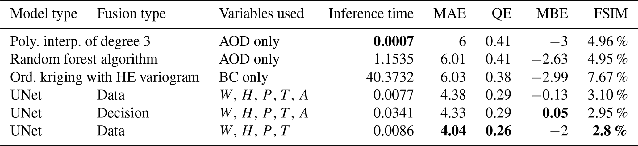
The polynomial interpolation method has a significantly smaller inference time than any other method discussed in this paper. However, this is the only metric on which one of the baseline methods outperforms our best results. Indeed, our models outperform the chosen baselines by a large margin in all metrics except this one. Our hybrid models do not appear in Table 6 as they are outperformed by the models presented in this table. However, as stated in Sect. 6.5, their performances remain comparable. In other words, our hybrid models are outperformed by the models presented in Table 6, but not by a large margin.

It has already been stated that, in a context where ground truths are less available, GANs outperform UNets. Indeed, their usefulness for this problem lies in their ability to realise semi-supervised learning. It is also interesting to note that generally speaking, all models would probably benefit from a larger amount of data as long as the training set remains representative of the actual data in a real-case scenario. The representativity of the dataset is paramount as it helps avoiding the overfitting problem often encountered in machine learning. More specifically, our deep learning models are the ones that would benefit the most from a larger amount of accessible data as they contain more parameters.

7 Conclusion

In this paper, we perform an extensive study on the use of several meteorological variables and column aerosol optical properties as inputs for a deep learning model to infer PM_2.5 concentrations from AOD using a scaling approach applicable globally. We tested different network architectures as well as the use of three different fusion strategies for the exploitation of these inputs in order to investigate the optimal way of fusing those information for our specific application. Hybrid methods of fusion have been proposed, implemented and studied as well. Our experiments were conducted extensively on CAMS data in order to assess model performances at global scale. We also performed a limited experiment using the ALADIN dataset (instead of CAMS) over a large region covering Europe and the Mediterranean basin to study the impact of the datasets' characteristics on our results, especially its spatial resolution and geographic spatial coverage.

Based on five metrics used throughout to evaluate different models performances, our experiments have shown the superiority of UNets over BC-GANs in our context, as is shown by Fig. 8. However the sparse training set is, in our context, significantly smaller than the complete set. We suggest in Sect. 6.1 that this induces a reduced need for semi-supervised learning and explains the difference in performance between UNets and GANs. The authors of Dabrowski et al. (2023) show the superiority of their BC-GANs over UNets in their context, which includes sparse and complete training sets of a more comparable size. This shows that the difference in performance between BC-GANs and UNets is not inherent to these models themselves. Therefore, we recommend the use of a UNet in our context of semi-supervised learning, with our sparse training set being significantly smaller than our complete training set. It remains difficult to deduce superiority of one model over the other in the general sense from our experiments. The comparison between our results and the results of Dabrowski et al. (2023) does show that the quantity of sparse data has a significant impact on the performances of these two models. Therefore, this context parameter must be taken into account when recommending one of these models over the other.

Our results have also illustrated that increasing the number variables as input tends to augment model performances. This is not surprising as the limited set of variables we used were selected for their known influence on PM_2.5 surface concentration. This remains a tendency, however, and not a guarantee as some exceptions have been observed where, depending on network architecture and fusion strategy, adding a variable may degrade performance. This is interesting because it is counter-intuitive to the general belief that using more (relevant) data in deep learning yields better results and emphasises in particular the interest in studying the impact of network architecture for atmospheric applications.

Our experiments have also shown in Sect. 6.3 the importance of the dataset's characteristics (here spatial resolution and coverage) and its impact on not only the results but also the conclusions that can be drawn from them as well. This is especially important in atmospheric sciences because geophysical variables have different scales of variability, and network architecture should ideally be aligned with the spatial characteristics of input fields. Our work suggests that more work is needed to understand the impact of networks' architecture on their ability to fully capture spatial features that are specific to atmospheric sciences.

While identifying precisely the impact of each variable on the models' performances would be useful, the observations made in Sect. 6.4, and drawn from our results, highlight the difficulty of such a task.

The two fusion strategies that lead to our best results (shown in Sect. 6.2) are the data and decision fusion ones. According to our experiments, the data fusion strategy also seems to lead to more stable results. Moreover, it allows for building smaller models, which in turn leads to shorter inference times and training times.

Our experiments on hybrid models did not show clear evidence of their advantage compared to other models even though they do present comparable performances, as shown in Sect. 6.5. Based on these conclusions, the data fusion strategy is the one we would recommend in a general case when all input variables are available at the same resolution and over the same area. Of course, this recommendation depends on general context and more specifically on the definition of the desired outcome. For example, using different metrics to measure performance might lead to a different recommendation.

Finally, our objective was not to develop a single and optimised model for PM_2.5 inference from AOD but rather to study how multiple PM_2.5 predictors could be used in order to best align the network architecture with the seek inference function. However, while we did not try to conduct specific optimisation and used only a limited set of predictors, we propose several architectures that yield PM_2.5 inference performances comparable to other tailored models found in the literature (Ma et al., 2022; Unik et al., 2023). The demonstrated performances obtained here should only be interpreted as baseline capabilities of the proposed models that could most likely be improved by extending further the time coverage of the learning database. As suggested by Zhou et al. (2024), we also strongly encourage a more systematic evaluation of models against a common test dataset and using standardised metrics. Since the code and data used for this article are both available, we suggest that our current results be seen as a benchmark for the task and context presented in this paper. Such a benchmark could be used as common ground for the evaluation of newly developed models of PM_2.5 inference AOD data, therefore facilitating their comparison.

As stated before, the experiments realised in this paper clearly illustrate the appeal of using additional, carefully chosen, input variables in order to augment the performance of a scaling model to infer PM_2.5 from AOD. Here we select a limited number of meteorological variables and optical properties that are well known to drive surface level PM_2.5 concentration. These variables are typically useful for establishing the link between PM_2.5 and AOD through a purely physics-based model, and, not surprisingly, our results demonstrate they are useful to establish this link through an artificial neural network. Based on this insight, an interesting possibility of future work consists of applying the concept of physics-informed neural networks (described in detail in Appendix A) to this problem and study depending of the fusion strategy used, at which level the incorporation of physics equations would be most relevant.

Appendix A: Related works

A1 Generative adversarial networks (GANs)

Since the authors of Goodfellow et al. (2020) proposed this type of model, the popularity of GANs has increased consistently. They rely on the training of two networks: a generator and a discriminator. The discriminator is presented with samples which can be either taken from the original data distribution or generated (by the generator). Its main task is to differentiate between these two kinds of inputs. On the other hand, if the discriminator makes an error and classifies a generated sample as real, then the generator is getting closer to its goal. The discriminator and generator's losses are built in such a way that when one increases, the other decreases, and reversely. This why they are called adversarial networks.

Convolutional GANs are known for their ability to produce realistic images, which can fool both their discriminator but also, in some cases, humans. They have also shown interesting performance in image-to-image translation tasks (Wang et al., 2019, 2020; Zhu et al., 2017b). This type of task is usually categorised as paired image translation, such as in Isola et al. (2017), or unpaired image translation, such as in Zhu et al. (2017a). In this article, our image translation task is a paired one.

A2 Explainable artificial intelligence (XAI)

Even though this work can not be classified as belonging to the field of XAI, the terminology this field proposes remains interesting in the context of this work. The general idea behind XAI is to build models that can be understood by their users or whose results can. While this field has existed for several decades (Confalonieri et al., 2021), its recent growth in popularity can be seen as a response to concerns about the black-box aspect of some neural networks models. This growth has been particularly remarkable in applications fields like finance, medicine, law and even scientific production (Beckh et al., 2021; Murdoch et al., 2019; Belle and Papantonis, 2021; Roscher et al., 2020). In those fields, the ability to explain a model and its results can represent the ability to ensure safety, fairness or scientific rigour. In a more general sense, it makes it easier for the user to trust the model.

According to Roscher et al. (2020), in the context of XAI, there are three important elements to consider when evaluating the explainability of a model.

1. Transparency. A model is transparent if the processes that extract model parameters from training data and generate labels from testing data can be described and motivated by its designer.

2. Interpretability. It is the ability to generally understand what the model bases its decisions on. Some approaches for interpretable models are based on decision trees as they can allow for an intuitive look at the decision-making process of a model.

3. Explainability. An explanation is the collection of features of the interpretable domain that have contributed to a given example to produce a decision. For a model to be explainable, it generally needs to be possible to understand why the model's decision for a given datum A is different than for a given datum B.

It is interesting to note that domain knowledge can be used to enhance the explainability of a model (Beckh et al., 2021). In this sense, physics-informed neural networks can be seen as a type of XAI.

A3 Physics-informed neural networks (PINNs)

Physics-informed learning, introduced by the authors of Raissi et al. (2019), can be considered today to be its own research field. The term informed networks suggests that the method makes use of prior information about some specificity of the problem, for example, its geometry. Physics-informed networks specifically make use of the physics of the problem to enhance their performances. This is usually done through the design of a physics-informed loss function, used during the training of the model. This loss function is often based on a differential equation that is verified by the data the model is using. As it can sometimes guide the training in a non-data-oriented way, the use of this loss function reduces the need of these networks for labelled data, making them especially suitable for semi-supervised learning.

In physics, it is often necessary to use initial and boundary conditions (BCs) to solve a given problem. In the literature around physics-based learning methods, two methods to take these BCs into account during training can be found. The soft constraint (or method) proposes to train the model to respect the BCs through the use of an additional, tailored loss function. The hard constraint (or method) works through the transformation of the model outputs to enforce the respect of the BCs and relies on pre-existing loss functions. When it comes to PINNs, the authors of Sun et al. (2020) show that the hard constraint performs better than the soft one.

Several authors have proposed to leverage the advantages shown by both adversarial and physics-informed approaches (Thanasutives et al., 2021; Nie et al., 2021), often calling these new models PI-GANs (Yang et al., 2019, 2020).

A4 Kriging method

This spatial interpolation and extrapolation method was formalised by the author of Matheron (1963). In the statistical interpretation of the term, it is the optimal estimation method according to Gratton (2002). It is mathematically described by Eq. (A1).

$$\begin{array}{}\text{(A1)}& F\left(x_p\right)=\sum _{i=\mathrm{1}}^m{W}_i\cdot F\left(x_i\right)\end{array}$$

F(x_p), the value of function F at point x_p can be estimated thanks to m surrounding points x_i as the value of F at these points is known. However, it remains necessary to determine the weight W_i of these points. The kriging method proposes to realise this through the estimation of what is called a variogram. To compute it, values of the variance of two points, and of the distance between them, are needed.

This method has been described as performing better when provided with a significant volume of data and when the values to estimate are following a normal distribution.

For each inference, a new point x_i is used. As these points are the basis for the building of the kriging model, a new one is built for each inference. Because of this, kriging suffers from a long inference time when compared to other methods presented in this article.

Appendix B: Details of the approach

The purpose of this section is to show the architecture of GAN's discriminator with our three main fusion strategies.

B1 Data fusion/channel concatenation

Figure B1 shows GAN's discriminator's architecture with the data fusion strategy.

Figure B1 Architecture of GAN's discriminator with data fusion approach.

B2 Feature fusion

Figure B2 shows GAN's discriminator's architecture with the feature fusion strategy.

Figure B2 Architecture of GAN's discriminator with feature fusion approach.

B3 Decision fusion

Figure B3 shows GAN's discriminator's architecture with the data fusion strategy.

Figure B3 Architecture of GAN's discriminator with decision fusion approach.

Appendix C: Model complexity

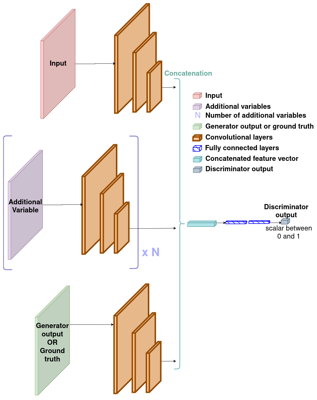
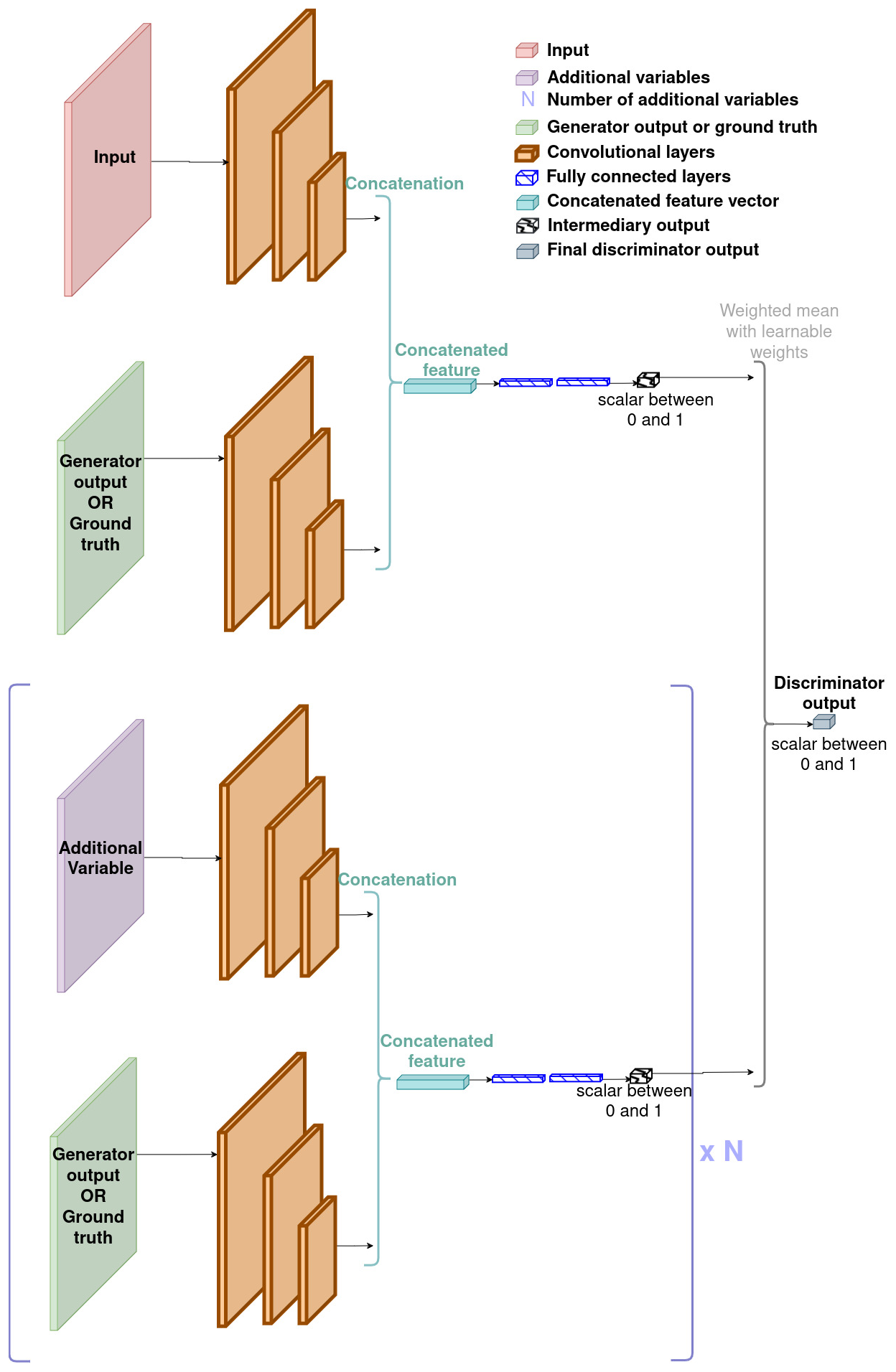
Figure C1 shows the number of parameters of our models depending on the fusion method and the number of input images used. They correspond to the number of parameters for our UNets and BC-GANs, with both ALADIN and CAMS data.

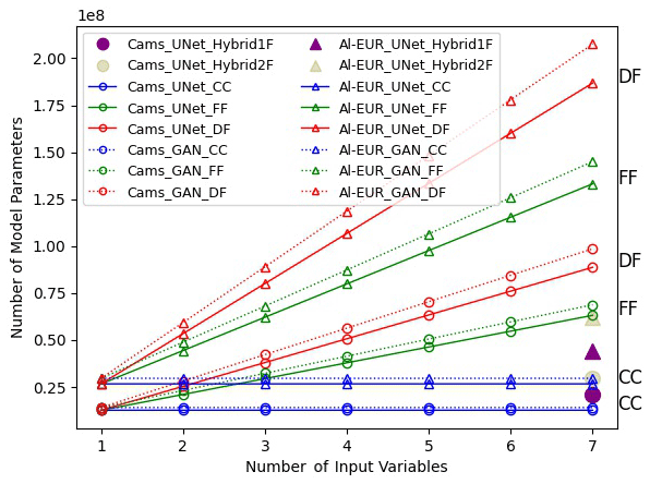
Figure C1 Number of parameters of each of our models depending on the number of input variables.

Appendix D: Training loss, test loss and convergence

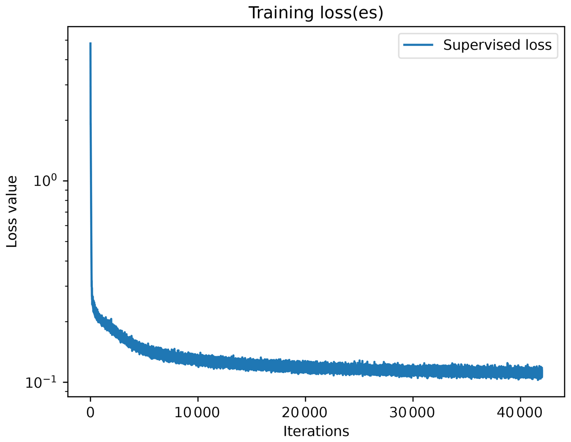
Figure D1 provides a graph of training loss values over iterations, clearly showing the convergence of the model. This corresponds to the training of a UNet model using exclusively the AOD as input. In this experiment, as in all other experiments presented in this article, the models are trained on 500 epochs.

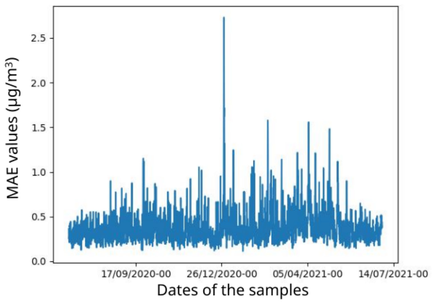
Figure D2 gives, for the same model, an overview of the MAE values for the different test samples. A few test samples stand out as having a significantly worse MAE than others, but the maximum MAE for these samples remains below 3 µg m⁻³, which is satisfying.

Figure D1 Graph of training loss during supervised learning over iterations.

Figure D2 Graph of MAE values during testing over sample date.