The Tropical Basin Interaction Model Intercomparison Project (TBIMIP)

Large-scale interaction between the three tropical ocean basins is an area of intense research that is often conducted through experimentation with numerical models. A common problem is that modeling groups use different experimental setups, which makes it difficult to compare results and delineate the role of model biases from differences in experimental setups. To address this issue, an experimental protocol for examining interaction between the tropical basins is introduced. The Tropical Basin Interaction Model Intercomparison Project (TBIMIP) consists of experiments in which sea surface temperatures (SSTs) are prescribed to follow observed values in selected basins. There are two types of experiments. One type, called standard pacemaker, consists of simulations in which SSTs are restored to observations in selected basins during a historical simulation. The other type, called pacemaker hindcast, consists of seasonal hindcast simulations in which SSTs are restored to observations during 12-month forecast periods. TBIMIP is coordinated by the Climate and Ocean – Variability, Predictability, and Change (CLIVAR) Research Focus on Tropical Basin Interaction. The datasets from the model simulations will be made available to the community to facilitate and stimulate research on tropical basin interaction and its role in seasonal-to-decadal variability and climate change.

1 Introduction

Interaction between the tropical basins on interannual to decadal timescales has seen increased interest in recent decades. This is partly due to the growing awareness that this interaction substantially influences variability in all three tropical basins (Cai et al., 2019; Wang, 2019) and that it may also shape the way in which the climate system reacts to radiative forcing, particularly that associated with changing greenhouse gas concentrations (Kosaka and Xie, 2013; Li et al., 2016). Furthermore, there is evidence that the linkages between the three tropical basins will change under global warming, leading to the emergence of new processes in the climate system, such as the tropical Atlantic influence on El Niño–Southern Oscillation (ENSO; Rodriguez-Fonseca et al., 2009; Martin-Rey et al., 2014; Polo et al., 2015; Wang et al., 2024a) or that of the Indian Ocean on ENSO (Wang et al., 2024b).

Research on interbasin interaction has undergone several phases. In the 1970s and 1980s, many researchers focused on understanding the mechanisms of ENSO in the tropical Pacific and the air–sea coupling that underlies it (e.g., Bjerknes, 1969; McCreary, 1976; Rasmusson and Carpenter, 1982; McCreary and Anderson, 1984; Philander, 1985; Zebiak and Cane, 1987). Over time, there was increasing interest in how ENSO influences other terrestrial and oceanic regions around the world (e.g., Bjerknes, 1969; Horel and Wallace, 1981; Karoly, 1989; Kiladis and Diaz, 1989; Enfield and Mestas-Nuñez, 1999; Klein et al., 1999; Diaz et al., 2001; Alexander et al., 2002). During this stage, the focus was on remote influences from the tropical Pacific to other regions. At the same time, other tropical ocean regions received increasing attention, which led to the discovery and analysis of other tropical variability patterns, such as the Atlantic Zonal Mode (AZM; Moore et al., 1978; Hastenrath and Heller, 1977; Merle, 1980; reviews by Lübbecke et al., 2018; Richter and Tokinaga, 2021), the Indian Ocean Basin Mode (IOBM; Chambers et al., 1999; review by Schott et al., 2009), and the Indian Ocean Dipole (IOD; Saji et al., 1999; Webster et al., 1999; review by Schott et al., 2009). Several variability patterns in the subtropics also became more prominent, such as the Atlantic Meridional Mode (AMM; Hastenrath and Heller, 1977; Chang et al., 1997; reviews by Xie and Carton, 2004, and Chang et al., 2006a), the Benguela Niño (Shannon et al., 1986; review by Oettli et al., 2021), the Ningaloo Niño (Feng et al., 2013; review by Tozuka et al., 2021), and the North Pacific Meridional Mode (NPMM; Chiang and Vimont, 2004; review by Amaya, 2019), to name a few. Increasingly, the question arose as to what extent variability in those remote regions was independent of ENSO and whether it could influence the evolution of ENSO (see Chang et al., 2006a, for a review, and Fig. 1 for a schematic). Thus, there was a growing interest in how the tropical oceans interact and how these interactions may contribute to improved seasonal predictions of oceanic variability patterns and their impacts over land (Keenlyside et al., 2019).

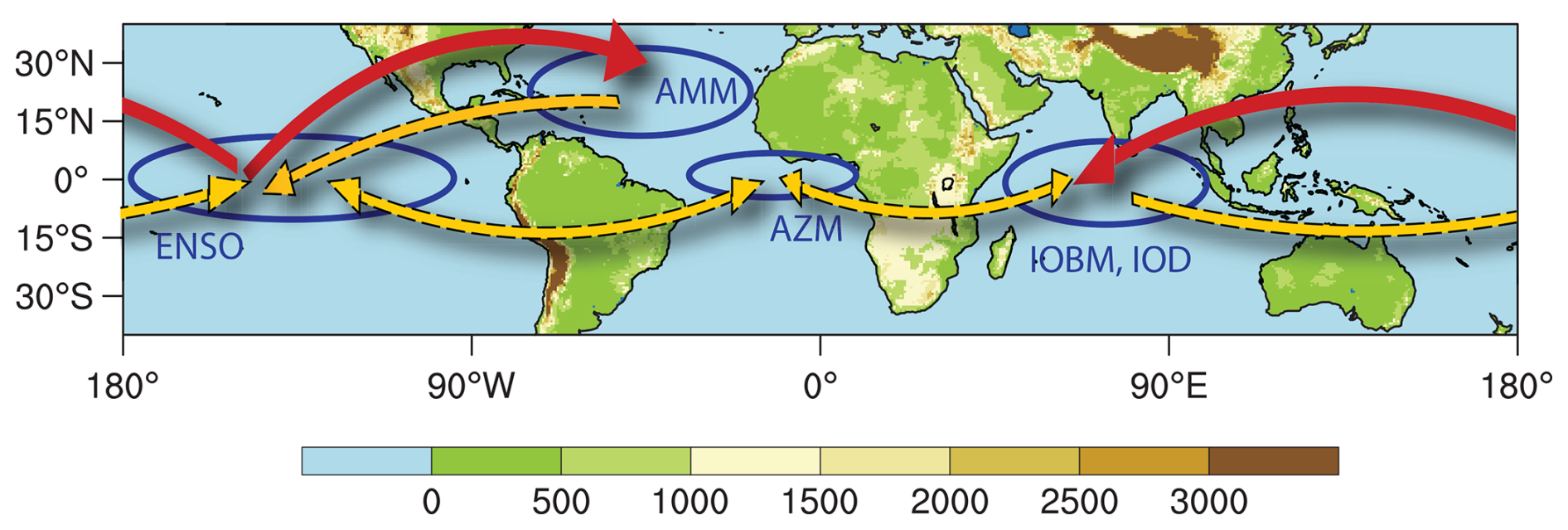
Figure 1 Schematic illustrating the interaction of selected tropical variability patterns, i.e., ENSO (El Niño–Southern Oscillation), AMM (Atlantic Meridional Mode), AZM (Atlantic Zonal Mode), IOD (Indian Ocean Dipole), and IOBM (Indian Ocean Basin Mode). The arrows illustrate the directionality of the influence and are not necessarily representative of the actual interaction pathways. The AZM-to-ENSO influence, e.g., could be through atmospheric equatorial Rossby waves, as suggested by the arrow, or atmospheric equatorial Kelvin waves (not indicated). The solid red arrows show well-established influences, while the dashed yellow arrows show influences that are under debate or inconsistent. The shading shows topographic heights (m) from the Earth topography 5 min grid (ETOPO5; National Geophysical Data Center, 1993), with ocean areas set to zero.

In addition to interannual variability patterns, such as ENSO, AZM, and IOD, there are also decadal and multidecadal variability patterns, both in the tropics (e.g., the Tropical Pacific Decadal Variability TPDV; see Power et al., 2021, and Capotondi et al., 2023, for a review and the decadal IOD as reported in Ashok et al., 2004, and reviewed by Han et al., 2014) and the extratropics (e.g., the Pacific Decadal Oscillation PDO; Zhang et al., 1997; Mantua and Hare, 2002; review by Newman et al., 2016) and the Atlantic Multidecadal Variability (AMV; Kushnir, 1994; reviews by Keenlyside et al., 2015, and Zhang et al., 2019). Due to their long timescales and extratropical locations, the latter patterns may influence other basins through different pathways (e.g., Ruprich-Robert et al., 2017). The associated background changes may also modulate the way in which ocean basins interact on shorter timescales (Yu et al., 2015; Martin-Rey et al., 2015; Kajtar et al., 2018; McGregor et al., 2018; Drouard and Cassou, 2019). In addition, suppressing tropical basin interaction (TBI) in numerical experiments has been found to shift ENSO variability to lower frequencies (e.g., Kajtar et al., 2017; Kido et al., 2022; Bi et al., 2022; Zhao and Capotondi, 2024). It should also be noted that some of the interannual variability patterns of interest have considerable variance at decadal timescales. These include the central Pacific El Niño (Sullivan et al., 2016) and the AMM (e.g., Chang et al., 2006a). Thus, the decadal and longer timescales are of interest to the study of TBI, but the observational record is short when low-frequency variability is the focus. The limited sample size of decadal-scale events, such as the AMV, as well as the existence of dedicated sensitivity experiments in the Coupled Model Intercomparison Project Phase 6 (CMIP6) Decadal Climate Prediction Project (DCPP; Boer et al., 2016), have motivated us to focus the proposed experiments on interannual timescales while still considering the role of decadal modulation of remote influences, e.g., that of the equatorial Atlantic on ENSO (Fig. 2).

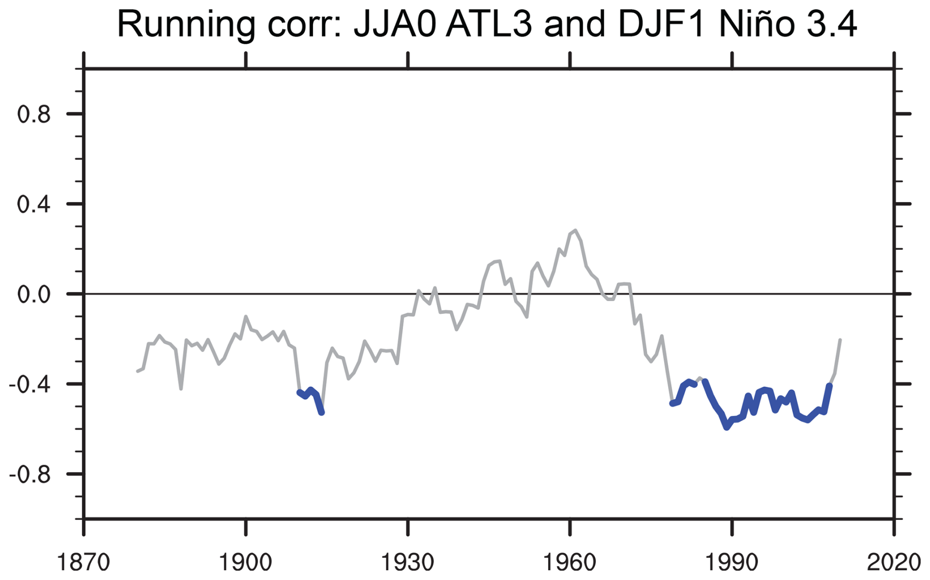
Figure 2 Running correlation of the June–July–August (JJA) ATL3 SST and the following December–January–February (DJF) Niño 3.4 SST using a 21-year sliding window for the period 1870–2021. The SST is from the CMIP6 amip experiment (see Sect. 3). Correlation significance at the 95 % level is indicated by the thick-blue-line segments. The significance test evaluates the null hypothesis that the correlations are due to chance, using bootstrapping with 10 000 samples generated by randomly reshuffling 1-year blocks (Wilks, 1997). The figure suggests a strengthening of the equatorial Atlantic influence on ENSO since the 1970s, as suggested by Rodriguez-Fonseca et al. (2009), and a potential weakening at the end of the analysis period. Some of the experiments proposed for TBIMIP can address the potential dependence of such modulations on changes in background state, SST anomaly patterns, and radiative forcing.

To study TBI, observational analysis is an obvious tool. Unfortunately, the observational record is relatively short, as mentioned above, with about 60–70 years of reliable data. For ENSO, e.g., this translates into roughly 20–30 events, and even fewer if only major events are considered. Given the considerable event-to-event diversity of ENSO (e.g., Timmermann et al., 2018), it is clear that the length of the observational record is a serious limitation when addressing interbasin interaction, particularly for statistical analysis and causality assessments. The event-to-event diversity increases further when considering the variability patterns in all three tropical ocean basins. A La Niña event, for example, may be accompanied by a positive AZM event in one year, by a negative IOD in another, and by a combination of a positive AMM and a positive IOD in yet another. Thus, every year in the observational record features its own unique constellation of variability patterns in the three ocean basins, rendering the seemingly long 70-year observational record insufficient for disentangling the complex interactions. This is only complicated by the long-term changes in radiative forcing during the observation period.

Paleo-proxies can substantially extend the data record available for analysis and have been used in the study of TBI (e.g., Cobb et al., 2001; Leduc et al., 2007). Proxy data, such as the water isotope ratio, however, must be converted into variables of interest using a number of assumptions, which can contribute to uncertainties. Furthermore, the temporal resolution of such records may not always be high enough to resolve the variability patterns of interest, particularly when data for a particular season are desired. There is also uncertainty associated with the dating of proxies. Finally, the spatial coverage is sparse, particularly in the tropical Atlantic.

Climate model experiments offer several advantages, such as long simulations (1000 years or more) under steady radiative forcing, as is the case for the preindustrial control simulations of CMIP6 (Eyring et al., 2016). In addition, climate model simulations allow experimentation, such as prescribing sea surface temperatures (SSTs) in one basin and analyzing the response in other basins. This avenue of investigation has been pursued by many groups, and numerous papers have been published (see Cai et al. (2019) for a review). Some of these studies, however, have arrived at diverging results. There is, e.g., disagreement on the role of the tropical Atlantic in influencing ENSO evolution, as illustrated by the composite of positive AMM events (Fig. 3), based on the SST from ERA5 (Hersbach et al., 2023). Some studies argue for a strong influence (e.g., Rodriguez-Fonseca et al., 2009; Ding et al., 2012; Ham et al., 2013a, b; Martin-Rey et al., 2015), others for a limited influence (Exarchou et al., 2021; Richter et al., 2021; Richter et al., 2023; Zhao and Capotondi, 2024), while some other studies dismiss this influence as a statistical artifact (Zhang et al., 2021; Jiang et al., 2023). Both the atmosphere and ocean allow for interaction pathways through material flow and waves, and these pathways have no built-in directionality. That is, if the Pacific can influence the Atlantic, then the Atlantic can influence the Pacific. However, given the size of the Pacific basin and the amplitude of ENSO, it is valid to question the importance of outside influences on ENSO. This is one of the motivations for the TBI experiments described here.

Figure 3 ERA5 SST anomalies in the northern tropical Atlantic (NTA; 40–10° W, 10–20° N; green line) and Niño 3.4 (blue line) regions, composited on positive AMM events, which are defined here as SST anomalies in the NTA region exceeding 0.8 standard deviations in March–April–May. The years 1979, 1980, 1981, 1983, 1987, 1988, 1997, 1998, 2005, and 2010 are selected by this criterion. Values significant at the 95 % level are marked by dots (note that none of the Niño 3.4 values is significant). The composite shows that NTA events tend to be preceded by El Niño events, a well-known remote impact of ENSO (indicated by the curved red arrow; Enfield and Mayer, 1997). Furthermore, there are weak La Niña conditions in the winter following the peak of the positive AMM event. This has been interpreted as the NTA influencing ENSO (dashed curved red arrow; Ham et al., 2013a, b), but some studies have challenged this, including Zhang et al. (2021), who suggest that the apparent influence stems from a misinterpretation of ENSO's intrinsic phase reversal (i.e., El Niño events tend to be followed by La Niña, regardless of any tropical Atlantic SST anomalies; curved grey arrow). The experiments proposed for TBIMIP will allow evaluation of the importance of the NTA influence on ENSO.

There is also an enduring conundrum as to why the strong ENSO signal in boreal winter has a robust influence on the northern tropical Atlantic in spring (Enfield and Mayer, 1997) but an inconsistent influence on the adjacent equatorial Atlantic in summer (Chang et al., 2006b; Lübbecke and McPhaden, 2012). While some robust impacts on the equatorial Atlantic have been identified (Tokinaga et al., 2019; Jiang et al., 2023; Richter et al., 2024), it is still not fully understood why the major 1982–1983 and 1997–1998 El Niños were followed by negative and positive AZM events, respectively (Fig. 4). Finally, the relationship between ENSO and the IOD has been probed in various climate model experiments, and these have arrived at conflicting results, with some arguing for an IOD that is mostly independent of ENSO (e.g., Behera et al., 2006), one that may even influence ENSO (Behera and Yamagata, 2003; Luo et al., 2010), and others an IOD that is largely controlled by ENSO (e.g., Stuecker et al., 2017a). Recent work has also indicated that different flavors of the Indian Ocean Basin mode can alter the decay of El Niño events (Wu et al., 2024).

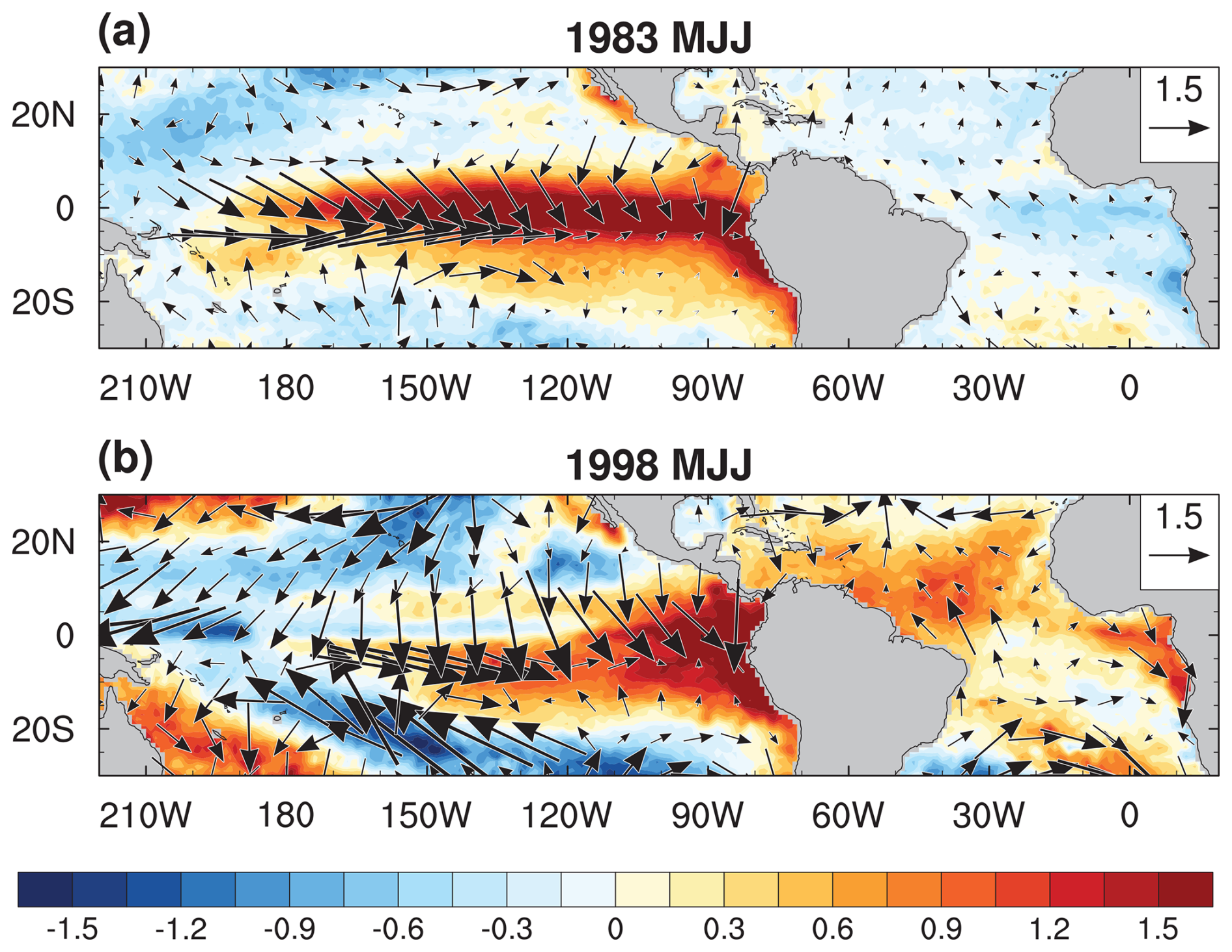
Figure 4 Anomalous SST (shading; °C) and 10 m winds (vectors; reference 1.5 m s⁻¹) averaged over May–June–July (MJJ) for (a) 1983 and (b) 1998. The fields are from ERA5 (Hersbach et al., 2023; note that SST is not an assimilated variable but a blend of various observational products). The remnants of the very strong 1982–1983 and 1997–1998 El Niño events are evident in the warm tropical Pacific SST anomalies. In the equatorial Atlantic, in contrast, SST anomalies have the opposite sign during those 2 years.

There are at least two reasons why different models may provide conflicting results. One is that experiments by different groups follow different protocols. This may include the way in which perturbations are implemented in the model code, but also different simulation and analysis periods. The other one is that systematic model errors (e.g., due to the use of different convective parameterizations) substantially influence the outcome of such experiments. Since such errors differ widely across models, the outcome of two sensitivity experiments conducted with different models can yield conflicting results, even if they follow the same protocol.

The proposed experiments can be categorized as “pacemaker” experiments, in which the atmospheric surface heat flux is modified to constrain the model SSTs to follow observations. Hereafter, we will refer to this simply as SST restoring. The overarching goal of the pacemaker experiments proposed for TBIMIP is to gain a deeper understanding of TBI and its potential role in seasonal-to-decadal predictions. This includes a better understanding of the pathways involved and their relative importance. Much of the interest in TBI stems from its potential to increase the skill of seasonal predictions, particularly that of ENSO and its global impacts. Quantifying the contribution of TBI to prediction skill is therefore one of the major goals of the TBI experiments, and a subset of the experiments is dedicated to this goal.

2 Justification for the Tropical Basin Interaction Model Intercomparison Project (TBIMIP)

While many experiments have been performed to explore TBI, these have followed varying experimental protocols, which makes it difficult to compare results, as discussed in Sect. 1. This was one of the major motivations for proposing an intercomparison project in which all models follow the same experimental protocol. Based on such coordinated experiments, it will be possible to evaluate the model dependence and robustness of the pathways of TBI.

Many general circulation model (GCM) intercomparison projects have been established, and their output is publicly available in many archives, most notably those of CMIP, which are hosted by the Earth System Grid Federation (ESGF). This prompts the question of whether there is a need for yet another intercomparison study. We first note that, while a wide range of intercomparisons have been performed, none of them has been dedicated to TBI on interannual timescales. The DCPP component of CMIP6 features some experiments that are related to TBIMIP. That project, however, focuses on decadal variability, while TBIMIP focuses on interannual variability. Since the AMV is one of the most pronounced patterns on decadal scales and longer timescales, most DCPP experiments are designed to examine AMV impacts. As such, they examine the impacts of AMV-related SST anomalies, which evolve slowly and extend into the high latitudes. The only experiment that partially overlaps with TBIMIP is the DCPP Tier-3 experiment “dcppC-pac-pacemaker”, in which SSTs in the tropical Pacific are restored to observations. In addition to only one model having performed this experiment, the DCPP's focus on decadal timescales means that the settings are not ideally suited to exploring interannual TBI. The Global Monsoons Model Intercomparison Project (GMMIP; Zhou et al., 2016) also features one experiment that is related to TBIMIP. In hist-resIPO, SST anomalies are restored to observations in the central and eastern tropical Pacific. Four models in the CMIP6 archive have completed this experiment, but the protocol differs from that of TBIMIP. Importantly, there are no corresponding experiments for the tropical Atlantic and Indian oceans. We thus believe that the TBIMIP experiments proposed here offer a unique opportunity to explore TBI and its role in climate variability. Due to its seasonal prediction component, TBIMIP will also offer an up-to-date dataset for comparing the prediction skill of state-of-the-art prediction systems.

While the proposed TBIMIP experiments are distinct from the DCPP experiments, they may provide complementary information regarding the role of tropical processes in decadal climate variability. Further synergy with existing CMIP6 experiments is provided by the use of the existing CMIP6 experiment “historical” as the reference for one subset of the proposed experiments, as explained in Sect. 3. This eliminates the need to run a separate control simulation, thereby reducing TBIMIP's computational load. It also allows comparison with the numerous experiments that are derived from historical and that are available in the CMIP6 archive, such as the single forcing experiments in the Detection and Attribution Model Intercomparison Project (DAMIP; Gillett et al., 2016).

3 Experiment design of TBIMIP

Here we describe the key details of the experiment design. The full description can be found at https://www.clivar.org/sites/default/files/documents/TBI_CoEx_design.pdf (last access: 5 December 2024) or https://doi.org/10.5281/zenodo.13864935 (Richter, 2024a). A summary of the Tier-1 and Tier-2 experiments is given in Table 1. Potential Tier-3 experiments are discussed in Appendix A1.

Table 1 Overview of the TBIMIP experiments. The latitudes refer to the core restoring regions. These are tapered off poleward over 10° buffer zones.

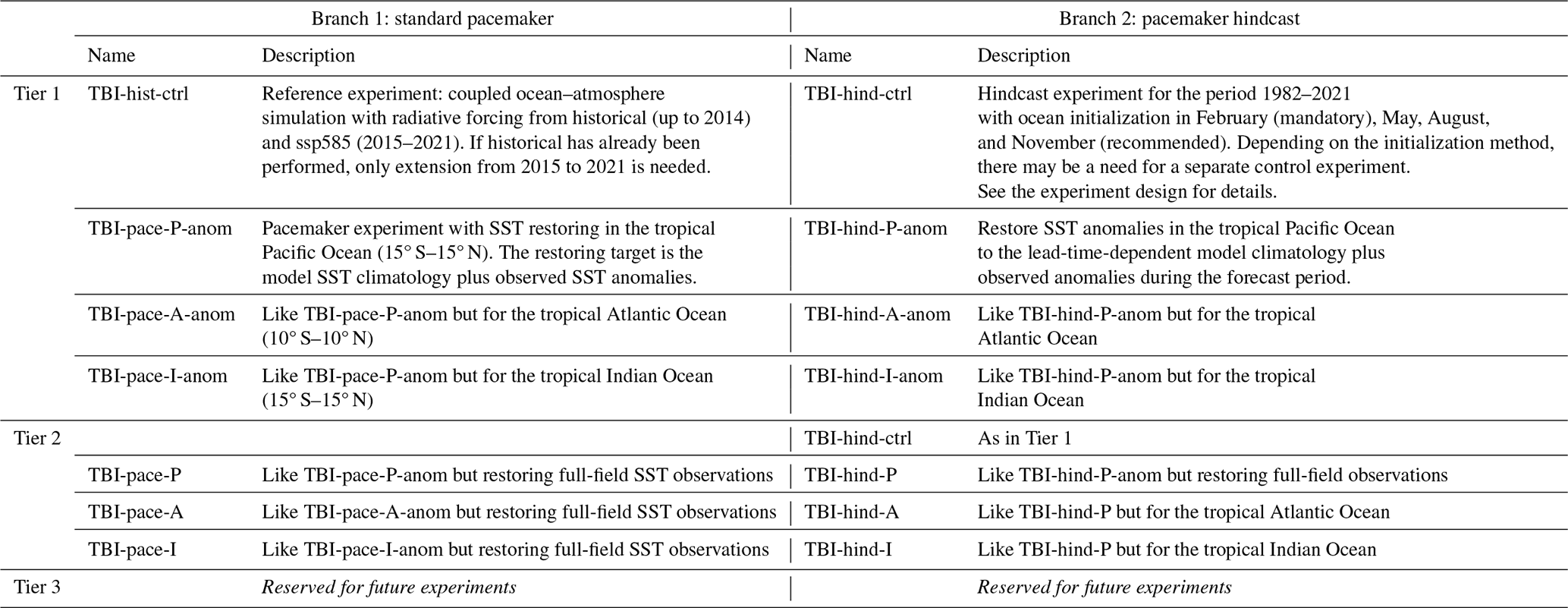
As in other MIPs, the experiments are grouped into three tiers, with Tier 1 having the highest priority. Experiments in this tier use the anomaly-restoring technique, while experiments in Tier 2 use full-field restoring to observations. Tier 3 is currently left to future additional experiments, which may be suggested by analysis of the Tier-1 and Tier-2 experiments. Several suggestions for such experiments are given in Appendix A1. Both Tier 1 and Tier 2 are divided into two sets, or branches, of experiments. The first branch consists of standard pacemaker experiments, which are continuous integrations over the historical period from 1982 to 2021 (starting from 1870 is recommended), with SST restoring in selected basins. The second branch consists of pacemaker hindcasts for the period 1982–2021. These are initialized seasonal predictions with SST restoring in selected basins. (We note that we use “hindcast” in the sense of “reforecast”, i.e., seasonal prediction experiments that are initialized from past observations.) Examples of such experiments can be found in the literature (e.g., Keenlyside et al., 2013; Luo et al., 2017). Participating groups can choose to perform only one of the two branches or both. For a given branch, however, all experiments should be performed.

Since the Tier-1 experiments use anomaly restoring, the SST target has to be calculated as the model SST climatology plus observed SST anomalies. The base period for calculating both the climatology and the anomalies is 1982–2019. The model climatology must be calculated from the reference simulation, which is TBI-hist-ctrl for the standard pacemaker and TBI-hind-ctrl for the pacemaker hindcast. For Tier 2, in contrast, the target SST is taken directly as the full-field observations.

The standard pacemaker experiments (branch 1) use the CMIP6 historical experiment as their control simulation. Groups that did not participate in CMIP6 should follow the CMIP6 protocol to perform the equivalent of historical. The radiative forcing is available via the ESGF website at https://pcmdi.llnl.gov/CMIP6/Guide/modelers.html (last access: 8 December 2024). Where a preindustrial control simulation (e.g., piControl in CMIP6) exists, a random year from that simulation should be chosen to initialize the control simulations. The CMIP6 forcing for the historical experiment is only available until 2014. It is suggested to use the radiative forcing from the ssp585 experiment for the period 2015–2021. However, since the radiative forcing does not vary much across scenarios for the first few years, any of these scenarios will be acceptable (Bi et al., 2022).

Three pacemaker experiments are requested, one for each of the tropical Pacific Ocean, the tropical Atlantic Ocean, and the tropical Indian Ocean. In each of these experiments, SSTs are restored to the target SSTs in the restoring region (10° S–10° N for the Atlantic Ocean and 15° S–15° N for the Pacific and Indian oceans; see Sect. 4.3 for a justification of the narrower restoring region in the Atlantic). The restoring is linearly tapered to zero over a 10° buffer zone to the north and south of the core restoring region. The restoring timescale should be 15 d over a 50 m layer. The target SST is based on the boundary conditions of the CMIP6 amip experiments (Durack and Taylor, 2016) but extended to December 2022 (Paul Durack, personal communication, 2023). The amip SST boundary conditions, in turn, are derived from the Hadley Centre Sea Ice and Sea Surface Temperature dataset (HadISST; Rayner et al., 2003) from January 1870 through October 1981 and the NOAA Optimum Interpolation SST (OISST) version 2 (Reynolds et al., 2002) from November 1981 through December 2022.

Masking has to be used to limit the SST restoring to the target basin. The restoring regions, including the tapering zones, are illustrated in Fig. 5. The core integration period for the standard pacemaker experiments is 1982–2021, but starting from 1870 is recommended to allow for more robust analysis. The experiments should be initialized from the control simulation (CMIP6 historical or equivalent) and use the same radiative forcing. A minimum of 10 ensemble members is recommended. The method for generating perturbed ensemble members is left to the modeling groups. One simple method is to slightly perturb the initial atmospheric temperatures.

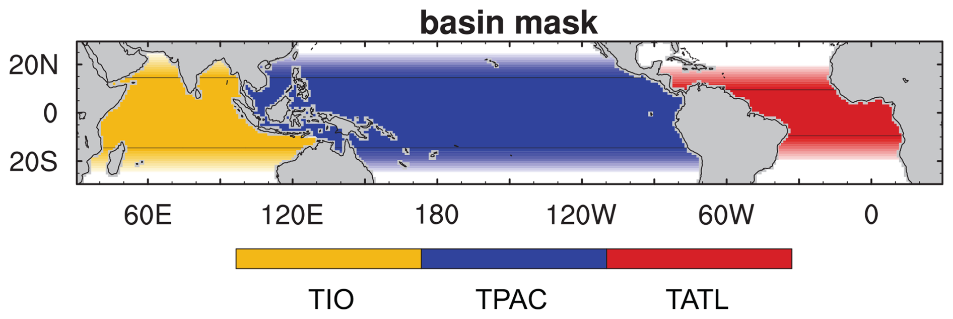
Figure 5 The basin mask to be used for the TBIMIP experiments. See the section on “Data and code availability” for how to obtain the data. The tropical Indian Ocean (TIO), the tropical Pacific (TPAC), and the tropical Atlantic (TATL) are indicated by yellow, blue, and red shadings, respectively. The core restoring regions are demarcated by horizontal lines and the transition zones by opacity gradients. Note the narrower meridional width of the tropical Atlantic restoring region.

The pacemaker hindcasts (branch 2) are hindcast experiments with SST restoring in a selected basin. The control experiment is a standard hindcast experiment. Many modeling groups may already have performed a hindcast experiment. Those who do not must first complete this before performing the pacemaker hindcast experiments.

The technique for initializing the hindcasts (data assimilation, etc.) is left to the modeling groups. While the initialization method may influence the forecast skill and spread, it is not expected to strongly affect relative changes in the pacemaker experiments, although future experiments should test this. The minimum requirement is one initialization on 1 February of each year from 1982 through 2021. Each integration should be at least 12 months long. Additionally, initializations on 1 May, 1 August, and 1 November are recommended. Finally, 1 March initializations may be useful for assessing prediction skill in the equatorial Atlantic, due to the seasonality of the AZM.

Three pacemaker hindcast experiments are performed, one for each basin. The initialization method should be the same as for the control hindcast. The restoring region and strength are the same as for the standard pacemaker experiments in branch 1. The SST restoring starts with the initialization and is maintained throughout the forecast period. As for the standard pacemaker experiments, a minimum of 10 ensemble members is recommended.

4 Climate model pacemaker experiments

4.1 Basic concept and rationale

At the heart of TBIMIP are coupled ocean–atmosphere experiments with SST restoring in selected target regions. Typically, the restoring target is a time-varying observed SST distribution, where SSTs will follow observations in the target region. In the wider sense of the meaning, pacemaker experiments can also restore to idealized SST distributions, such as a composite El Niño event, or a seasonal climatology. The general idea behind these pacemaker experiments is to examine the response of the atmospheric circulation and the subsequent impacts on the climate system outside the restoring region. A well-known example is the pacemaker experiment of Kosaka and Xie (2013), which examined how the global surface temperatures respond to prescribing SST in the central and eastern tropical Pacific. In particular, Kosaka and Xie (2013) were interested in how the tropical Pacific influences the evolution of the global temperature trend. Another example would be a pacemaker experiment in which SSTs are restored to observations in the tropical Atlantic in order to analyze the impacts of the tropical Atlantic on ENSO variability (e.g., Ding et al., 2012; Keenlyside et al., 2013; Exarchou et al., 2021; Liu et al., 2023). Such pacemaker experiments ask the question to what extent the climate system will follow the observed evolution if one of its components is forced to follow observations. Tropical SSTs are an obvious candidate for this kind of intervention due to their strong influence on the atmospheric circulation. Other fields, however, can also be subjected to intervention, such as the surface wind fields (e.g., Richter et al., 2012; Ding et al., 2014; Gastineau et al., 2019; Voldoire et al., 2019), which have a strong impact on the ocean circulation and the surface enthalpy flux.

4.2 Methodology for SST restoring

There are several methods for constraining SST to follow a target time series. Below we list three potential methods, but we recommend using method (2).

1. Temperature nudging inside the ocean model. SST corresponds to the temperature of the uppermost vertical level of the ocean component. One approach is therefore to add a correction term to the temperature equation of the ocean model that nudges the SST toward the target value. The strength of the term is proportional to the difference between the target and model SST. This approach is akin to ocean data assimilation and has been employed in TBI studies (e.g., Ding et al., 2012; Chikamoto et al., 2016) and for the initialization of prediction experiments (Keenlyside et al., 2005; Keenlyside et al., 2013).

2. Surface heat flux term. The top ocean level interacts with the atmospheric model component through a coupler routine (e.g., Craig et al., 2017), which regulates the exchange of fluxes between the atmosphere and ocean. Another approach for modifying SSTs is therefore to manipulate inside the coupler routine the heat flux that goes into the ocean, which is the method recommended for the TBIMIP experiments. The heat flux in tropical regions consists of four components: net surface shortwave radiation, net surface longwave radiation, latent heat flux, and sensible heat flux. Of these, sensible heat flux is usually chosen for adding the restoring flux (e.g., Kosaka and Xie, 2013).

3. Modifying SSTs “seen” by the atmospheric model. Because the flux coupler controls the SSTs that are “seen” by the atmospheric component, one can modify only this value, thereby “tricking” the atmosphere into reacting to a temperature that is different from the actual ocean SST. This approach leaves the ocean component completely unchanged (Richter and Doi, 2019). Furthermore, it allows the SSTs to exactly follow a given distribution (as far as the atmosphere is concerned), rather than approximating it through correction terms. A potential drawback is that this can lead to very unrealistic heat fluxes into the atmosphere (Wang et al., 2005).

Method (2) is recommended because it is commonly used and because it allows SST restoring of variable strength, rather than the prescribed SSTs of method (3). It should also be easier to implement than method (1), which requires modification of the ocean model thermodynamic equation.

4.3 Considerations when modifying the surface heat flux

When constraining SSTs using the surface heat flux method, as recommended for the TBIMIP experiments, several issues need to be considered.

First, one has to decide on the strength of the restoring flux. The ocean mixed layer is an important concept to consider because it is the layer that rapidly adjusts to the surface forcing. In the tropical oceans, a typical value for the mixed-layer depth (MLD) is 50 m. Using this as a reference MLD, and based on the temperature difference between the actual and target SSTs, one can calculate the flux that is needed to achieve the target SST over a certain timescale:

$$\begin{array}{}\text{(1)}& F=\left(T_{\mathrm{t}}-T_{\mathrm{m}}\right)\mathit{\rho }{C}_{\mathrm{p}}{\displaystyle \frac{\mathrm{MLD}}{\mathit{\tau }}},\end{array}$$

where F is the correction heat flux [W m⁻²], T_t is the target SST [K], T_m is the model SST [K], ρ is the density of seawater [kg m⁻³], C_p is the heat capacity of seawater [J K⁻¹ kg⁻¹], MLD is the mixed-layer depth [m], and τ [s] is the restoring timescale. Thus, the heat flux needed increases with the deviation of the model SST from the target SST, the MLD, and the inverse of the restoring timescale. It is clear from Eq. (1) that an instantaneous adjustment (τ = 0, i.e., perfect agreement with the target SST) would require an infinite heat flux. One must therefore compromise between correspondence to the target SST and a surface heat flux that is not overly disruptive. In the literature, a wide range of restoring timescales has been used. The SINTEX-F1 seasonal prediction model (Luo et al., 2005) uses restoring timescales from 1 to 3 d over 50 m as a simple data assimilation scheme for its forecasts. At the other end of the spectrum, restoring timescales of 30–60 d over 50 m are used for decadal variability experiments, such as the CMIP6 DCPP. The IPSL decadal forecast system uses SST nudging and a restoring timescale of 30 d as an assimilation scheme (Servonnat et al., 2015).

So, what are the reasons for not using short restoring timescales even though they allow for the highest correspondence to the target SST? There are two main reasons. First, for short restoring timescales, the heat fluxes required can lead to very unrealistic changes in the ocean circulation. Because the heat flux is absorbed in the top layer first, the immediate temperature response could lead to unrealistic changes in vertical stability and, consequently, vertical mixing. Second, overly strong restoring can lead to unrealistic behavior in regions where SST is primarily driven by the surface heat fluxes, rather than driving them (Frankignoul, 1985; Frankignoul et al., 1998). This applies not only to extratropical regions, but also regions of the Indian Ocean, western Pacific Ocean, and northern tropical Atlantic Ocean (Klein et al., 1999; Alexander et al., 2002; Wang et al., 2000). In that case, strong restoring can affect the lead–lag relationship of SST and surface heat fluxes and even change the sign of this relationship, as has been shown in the context of AMV pacemaker experiments. This, in turn, can lead to an inconsistent large-scale response where the SST-mediated changes in surface fluxes produce unrealistic diabatic atmospheric heating and teleconnection patterns (Ding et al., 2014). In particular, some studies suggest that the role of the subtropical North Atlantic may have been overestimated in experiments that performed SST restoring there (Kim et al., 2020; O'Reilly et al., 2023).

Figure 6 examines the influence of SST restoring strength by showing the lead–lag relation between SST and surface enthalpy flux (SHF) for several regions that range from the subtropical North Atlantic (Fig. 6a) to the equatorial Atlantic (Fig. 6d; see the figure caption for area definitions). ERA5 is compared to CMIP6 simulations with the MRI-ESM2-0 climate model from three different experiments: historical, with full ocean–atmosphere coupling; hist-resAMO (part of GMMIP), with relatively weak SST restoring (60 d over a 50 m layer) in the AMO region (core restoring region 5–65° N, 65–5° W, with 5° buffer zones in the meridional and zonal directions); and amip, with SST completely fixed. For both the reanalysis and the model simulations, the analysis period is 1979–2014. In all three off-equatorial regions (Fig. 6a–c), ERA5 shows the highest positive correlation when SHF leads SST by 1 month, indicating that SHF anomalies are driving SST anomalies (Frankignoul et al., 1998). The lowest negative correlation occurs when SHF lags SST by 1 month, with low values for the contemporaneous correlation. This behavior is reproduced well by the MRI-ESM2-0 historical simulations. This correspondence to ERA5 is slightly decreased in the hist-resAMO simulation, presumably due to the interference from the SST restoring. In the amip simulation, however, there are negative correlations for both SHF leading SST and SHF lagging SST, indicating that the model attempts to damp the SST anomalies at all times. This contrasts with both the reanalysis and the other model simulations and strongly suggests that the SST prescription disrupts the relation between SHF and SST.

Figure 6 Lead–lag correlation of anomalous SST and surface enthalpy flux (SHF; the sum of sensible and latent heat flux) for −6 to +6 months, with SHF leading SST for negative lags. Positive correlations indicate that positive SST anomalies are associated with SHF anomalies in the ocean. The data are from ERA5 (green line) and the MRI-ESM2-0 CMIP6 model for the experiments historical (blue line), hist-resAMO (orange line), and amip (brown line). The analysis period is 1979–2014 for all of the datasets. Filled circles indicate correlations that are significant at the 95 % confidence level. The individual panels show the following area averages: (a) subtropical North Atlantic (subtropical NAtl; 40–10° W, 20–30° N), (b) northern tropical Atlantic (NTA; 40–10° W, 10–20° N), (c) equatorial North Atlantic (eq. NAtl; 40–10° W, 5–10° N), and (d) ATL3 (20–0° W, 3° S–3° N).

In the equatorial Atlantic (Fig. 6d), conversely, there are no categorical differences across the four datasets, with both the reanalysis and the simulations showing negative correlations that are lowest around the contemporaneous correlation. This indicates that the ocean circulation drives SST anomalies, while the atmosphere damps them through SHF anomalies.

Given that SST restoring can lead to unrealistic fluxes outside the deep tropics, as suggested by Fig. 6, it is advisable to limit the meridional width of the restoring region. We therefore restrict the core restoring region from 10° S to 10° N in the tropical Atlantic and from 15° S to 15° N in the tropical Pacific and Indian oceans, with 10° transition zones in each hemisphere. The smaller meridional extent of the tropical Atlantic restoring region is motivated by the fact that deep convection is more confined around the Equator there and by studies indicating unrealistic fluxes in the subtropical North Atlantic when SSTs are restored there (Kim et al., 2020; O'Reilly et al., 2023).

An important choice to make is whether to use full-field or anomaly SST restoring. In full-field restoring, the target SST field is the total observed SST, i.e., the observed SST climatology plus the observed SST anomaly. In anomaly restoring, on the other hand, the target is the model climatology plus the observed SST anomaly. The advantage of anomaly restoring is that it preserves the model SST climatology in the restoring region, so that it remains consistent with the climatology outside the restoring region, thus reducing the effect of sharp gradients. In the equatorial and southern tropical Atlantic, models tend to have a pronounced warm bias (e.g., Richter and Tokinaga, 2020). Under such circumstances, prescribing the observed climatology will reduce the average SST in the region and may fundamentally change the way in which it interacts with other basins. Anomaly restoring therefore offers a way of avoiding undesirable side-effects of the SST intervention. One potential disadvantage in the context of a multimodel intercomparison is that the total prescribed SST values will be different for every model. This may make it more difficult to compare results across models. In addition, the method requires some consideration of how to calculate the target SSTs. To illustrate this, we introduce a few equations. The total model SST can be written as the sum of a climatology and an anomaly $T_{\mathrm{m}}={\stackrel{\mathrm{‾}}{T}}_{\mathrm{m}}+T_{\mathrm{m}}^{\prime }$, where the overbar denotes the seasonally varying climatology and the prime denotes the anomaly. Likewise, the total observed SST can be written as $T_{\mathrm{o}}={\stackrel{\mathrm{‾}}{T}}_{\mathrm{o}}+T_{\mathrm{o}}^{\prime }$. For anomaly restoring, the restoring target is the sum of the model climatology and the observed anomaly: $T_{\mathrm{t}}={\stackrel{\mathrm{‾}}{T}}_{\mathrm{m}}+T_{\mathrm{o}}^{\prime }$. An energy imbalance can occur in the model if there is a mismatch between the restoring target and the model SST of the free-running control simulation: $E=T_{\mathrm{t}}-T_{\mathrm{m}}={\stackrel{\mathrm{‾}}{T}}_{\mathrm{m}}+T_{\mathrm{o}}^{\prime }-({\stackrel{\mathrm{‾}}{T}}_{\mathrm{m}}+T_{\mathrm{m}}^{\prime })=T_{\mathrm{o}}^{\prime }-T_{\mathrm{m}}^{\prime }$. If this imbalance accumulates over the integration period, it can potentially change the SST distribution outside the restoring region and adversely affect the outcome of the pacemaker experiment. Such an imbalance can occur if the base period (used for the calculation of the climatology) is different between the model and observations, due to the warming trend during the historical period. It is therefore important to use a consistent base period when calculating the restoring target. Even with the same base period, however, an imbalance can occur if the base period is much shorter than the integration period. As an example, consider a case where we define the base period as 1982–2019 but perform the pacemaker experiment over the period 1870–2021. Both the model and the observed SST anomalies are calculated relative to the same 1982–2019 base period: $T_{\mathrm{m}}^{\prime }=T_{\mathrm{m}}-{\stackrel{\mathrm{‾}}{T}}_{\mathrm{m}}^{(\mathrm{1982}\to \mathrm{2019})}$ and $T_{\mathrm{o}}^{\prime }=T_{\mathrm{o}}-{\stackrel{\mathrm{‾}}{T}}_{\mathrm{o}}^{(\mathrm{1982}\to \mathrm{2019})}$, where, without loss of generality, we neglect the seasonal dependence of the climatology. The time-integrated imbalance then becomes

$$\begin{array}{}\text{(2)}& \begin{array}{rl}{\int }_{t\mathrm{1}}^{t\mathrm{2}}\mathrm{Edt}& ={\int }_{t_{\mathrm{1}}}^{t_{\mathrm{2}}}(T_{\mathrm{o}}^{\prime }-T_{\mathrm{m}}^{\prime })\mathrm{d}t={\int }_{t_{\mathrm{1}}}^{t_{\mathrm{2}}}(T_{\mathrm{o}}-T_{\mathrm{m}})\mathrm{d}t\\ & -{\int }_{t_{\mathrm{1}}}^{t_{\mathrm{2}}}({\stackrel{\mathrm{‾}}{T}}_{\mathrm{o}}^{(\mathrm{1982}\to \mathrm{2019})}-{\stackrel{\mathrm{‾}}{T}}_{\mathrm{m}}^{(\mathrm{1982}\to \mathrm{2019})})\mathrm{d}t,\end{array}\end{array}$$

where t₁ and t₂ denote the integration period of the pacemaker experiment. Noting that the second term on the right-hand side of Eq. (2) is constant, and dividing by the integration period, we obtain

$$\begin{array}{}\text{(3)}& \begin{array}{rl}{\stackrel{\mathrm{‾}}{E}}^{(t\mathrm{1}\to t\mathrm{2})}& ={\stackrel{\mathrm{‾}}{T}}_{\mathrm{o}}^{(t\mathrm{1}\to t\mathrm{2})}-{\stackrel{\mathrm{‾}}{T}}_{\mathrm{m}}^{\left(t\mathrm{1}\to t\mathrm{2}\right)}\\ & -\left[{\stackrel{\mathrm{‾}}{T}}_{\mathrm{o}}^{(\mathrm{1982}\to \mathrm{2019})}-{\stackrel{\mathrm{‾}}{T}}_{\mathrm{m}}^{(\mathrm{1982}\to \mathrm{2019})}\right].\end{array}\end{array}$$

If the integration period is equal to the base period (t₁= 1982, t₂= 2019), the imbalance equals zero. Nontrivial imbalances can arise when the integration period is substantially longer (e.g., 1870–2021, as in our example) and if the difference between the model and observed SST substantially changes over the longer period. In other words, problems arise when the simulated and observed SST trends are substantially different. We test this for a few selected models participating in the CMIP6 historical experiment (Fig. 7a), using as the observational reference the CMIP6 amip SST, which is derived from HadISST and OISST (see Sect. 3). The area average of SST over the tropical Pacific varies substantially across the models, with the warmest model being almost 1.5 °C warmer than the coldest model and the observations roughly in the middle. This bias spread, however, is of no concern for our experiments because the bias itself does not enter into the energy imbalance. The important question is whether the gap between a given model and the observations varies substantially over time. We therefore remove the time mean and re-plot the SST evolution (Fig. 7b). The curves are now more closely spaced, suggesting that the bias of a given model does not vary substantially over time, although the well-known trend overestimation at the beginning of the 21st century is evident (Kosaka and Xie, 2013; Wills et al., 2022; Beverly et al., 2024). We conclude that using a shorter base period should not lead to major imbalances, though this should be evaluated carefully for each model. Calculating the imbalance (term E in Eq. 3) yields the values shown in Table 2, where, unlike in Eq. (3), the shorter base period is 1977–2014 (rather than 1982–2019), because this is readily available in the CMIP6 historical simulations.

Table 2 Imbalance (K) incurred by using a base period (1977–2014) that is much shorter than the integration period (1870–2014) when calculating the model climatology and observed anomalies (see Eq. 3 for an explanation) in historical simulations of seven CMIP6 models, as indicated in the top row.

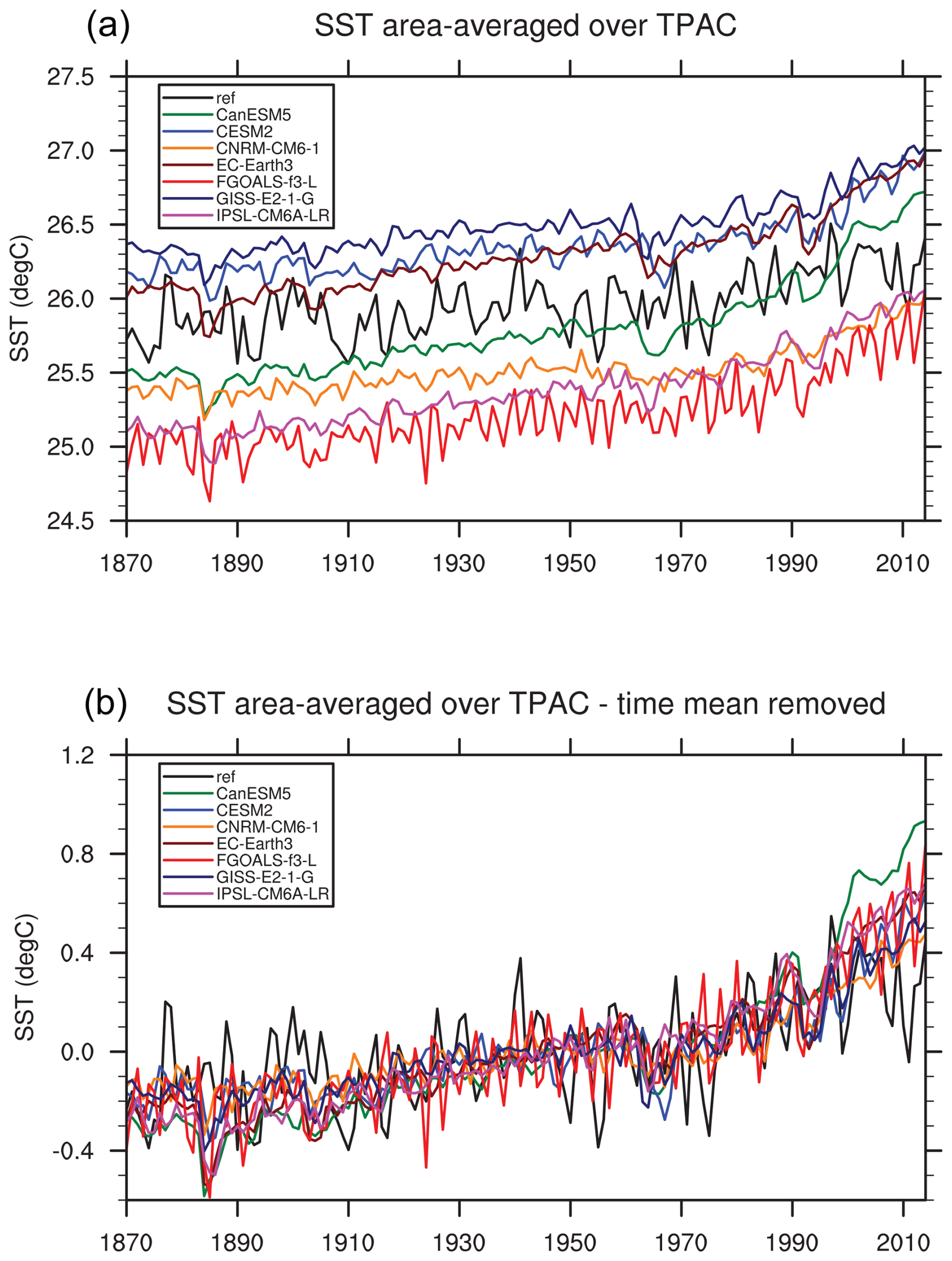
Figure 7 SST (°C) averaged over the tropical Pacific (entire basin width, 30° S–30° N) for the reference (CMIP6 amip SST) and seven models from the CMIP6 historical experiment, as indicated by the legend in the upper left of each panel. For the models, the lines represent the average over all the respective ensemble members. The panels show (a) the full-field SST and (b) the deviation of the full-field SST from its 1870–2014 time average for each dataset.

Following the above analysis, we define 1982–2019 as our base period. Using this relatively short base period for TBIMIP is motivated by the fact that it is a subset of the minimum period requested for all TBIMIP simulations. Thus, this period should be available to all participating groups. In particular, the pacemaker hindcast experiments (see Sect. 3) will only be performed for the period 1982–2021, meaning that a longer base period would not be possible for those experiments.

When restoring SSTs in a particular ocean basin, one has to consider not only the meridional extent but also the zonal extent of the restoring region. For the tropical Atlantic, the American and African coastlines provide an obvious choice for a basin mask. The boundary between the tropical Pacific and Indian oceans is not as obvious because the Indonesian Throughflow is a porous boundary. Some previous experiments have avoided this problem by excluding the entire western tropical Pacific (e.g., Kosaka and Xie, 2013). For TBIMIP, we choose to extend the tropical Pacific region all the way to the Maritime Continent, according to the basin mask provided by the World Ocean Atlas (Locarnini et al., 2010). Some modifications were performed to simplify the basin mask (Fig. 5). This mask is publicly available. See the “Data and code availability” section for how to obtain the data.

4.4 Drawbacks of pacemaker experiments

While pacemaker experiments are a useful tool for understanding the interaction between the tropical basins, they also have potential shortcomings.

1. The infinite heat source problem. SST restoring can lead to a potentially infinite heat source or sink. The larger the difference between the restoring target and the model SST, the larger the heat flux that has to be pumped into the ocean or atmosphere (see Eq. 1). This adjustment flux is a purely mathematical entity and therefore not bounded by any energy constraints. In practice, this issue will be more prominent when full-field restoring is used and when there are large model biases. Even in anomaly-restoring experiments, however, this issue can arise in regions where the atmosphere exerts an important influence on the ocean, such as in the subtropics. In such regions, the underlying assumption of SST pacemaker experiments that the SSTs drive the atmosphere is less valid, which can lead to unrealistic results, as discussed in Sect. 4.3.

2. Shift in the model dynamics. The intervention in the model dynamics may perturb the simulation to such an extent that it fundamentally alters the basic flow. In that case, interpretation of the results may be difficult. Again, this factor will be more important when full-field restoring is used.

3. Insufficient model fidelity. If the simulated variability patterns are substantially different from those observed, it may be difficult to draw conclusions about nature. One example would be the seasonal preference of variability patterns. ENSO, for example, is known to have its peak in boreal winter and models are known to struggle with reproducing this seasonal synchronization (Stein et al., 2014; Liao et al., 2021). If a model ENSO peaks in summer, for example, this may have serious repercussions for how it interacts with other basins. One of the reasons for TBIMIP is to study exactly this model dependence.

4. Incomplete decoupling of basins. While the goal of TBIMIP is to study the influence of individual basins on the climate system, this separation into individual basins cannot be completely successful. The SSTs one prescribes in the tropical Atlantic Ocean or Indian Ocean, for example, implicitly contain some impact from the tropical Pacific because ENSO has contributed to shaping them. It is therefore not possible to completely isolate the influences of individual basins, and this should be borne in mind when analyzing the output from pacemaker experiments. When assessing impacts on predictability, for instance, it has been shown that experiments with relaxation toward observations greatly overestimate ENSO forecast skill because of the built-in presumed perfect evolution of the stochastic noise-driven component of SSTs as well as the aforementioned ENSO effect on remote SSTs (see the discussion in Zhao et al., 2024).

5. Reliability of the observations. In addition to (1)–(4), which are limitations inherent to the modeling approach, there is also the problem of the reliability of the observations used to design the restoring target. This is mainly an issue for the pre-satellite era, when SST measurements mostly relied on shipboard observations. Thus, this issue can potentially affect the pacemaker experiments if they are extended beyond the satellite observation period. Results from this period will have to be treated with caution.

Despite the caveats listed above, we do believe that pacemaker experiments are a valuable tool for gaining a deeper understanding of TBI.

5 Participation

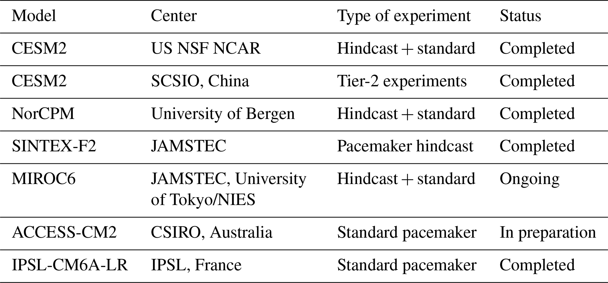
The participation of multiple modeling groups is essential for the success of any MIP. At the time of writing, several groups already completed the experiments, as detailed in Table 3. The participation of additional groups is greatly welcomed. The minimum requirement is the completion of at least one branch (standard pacemaker or pacemaker hindcast) of the Tier-1 or Tier-2 experiments. For the standard pacemaker branch, this consists of the control historical experiment and one experiment for SST restoring in each tropical basin. The minimum integration period is 1982–2021. Assuming 10 ensemble members, the minimum simulation time is 4 experiments × 10 ensemble members × 40 years per simulation, which equals 1600 simulation years. This reduces to 1200 simulation years if a historical simulation is already available.

Table 3 Status of the TBIMIP experiment execution as of February 2025. Unless explicitly noted, the status refers to Tier 1 experiments. “pmaker hindcast” and “hindcast” stand for the pacemaker hindcast branch, and “standard pmaker” and “standard” stand for the standard pacemaker branch of the experiments (see Sect. 3).

For the pacemaker hindcast experiments, the minimum requirement is one control hindcast experiment and one SST intervention experiment for each basin. The minimum hindcast period is 1982–2021, with at least one initialization per year (on 1 February) that is integrated for 12 months into the future. Thus, the minimum simulation time is 4 experiments × 10 ensemble members × 1 forecast initialization per year × 1 year per forecast × 40 years, which again equals 1600 simulation years.

The output variables that should be archived are listed in Table 4. They are grouped into three levels, with level 1 being the minimum requirement, level 2 desirable, and level 3 optional. The variable names follow the CMIP nomenclature, which can be found here: https://clipc-services.ceda.ac.uk/dreq/mipVars.html (last access: 19 May 2024). All variables need to follow the CMIP conventions, including the variable name and output format (“cmorization”). Vertical pressure levels for 3D atmospheric variables should follow the standard CMIP format (hPa), i.e., 1000, 925, 850, 700, 600, 500, 400, 300, 250, 200, 150, 100, 70, 50, 30, 20, 10, 5, and 1, with a reduced number of levels for daily data, as indicated in Table 4.

Table 4 Minimum requirements for output variables of the TBIMIP experiments in all three tiers and for both branches. The CMIP vocabulary for variable names is used. Variables that may not be included in the standard output of models are marked with an asterisk. If not indicated otherwise, monthly means are requested.

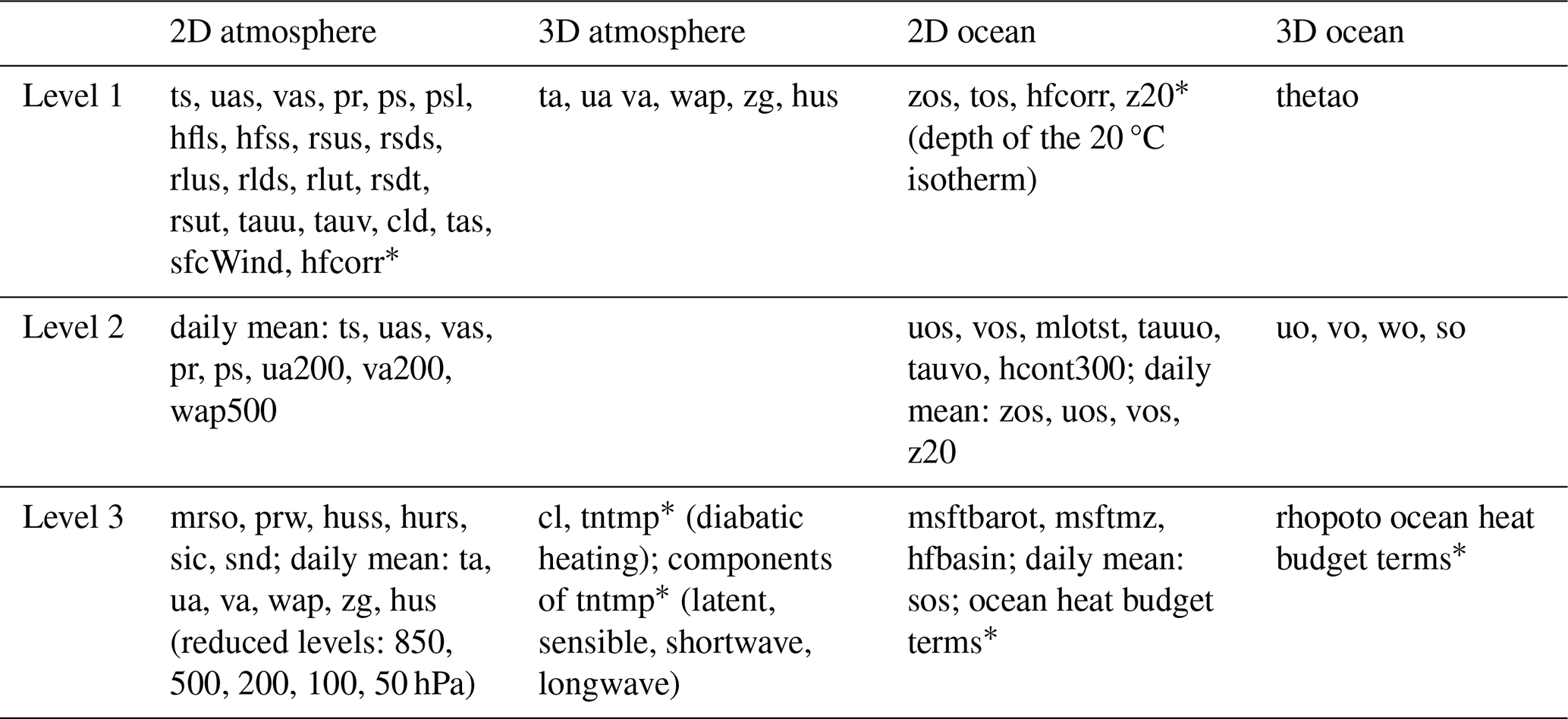
One variable that is only found in a few of the CMIP6 experiments is hfcorr, which is the heat flux term applied to restore SST to the target value. This is an important diagnostic for examining the potential energy imbalance created by the heat flux correction and is also a measure of how much the ocean SST would diverge from the target SST if left unperturbed, i.e., the degree to which the ocean–atmosphere system resists the SST restoring. In many models, outputting this variable will require code modifications. Note that this variable should be separate from the sensible heat flux or latent heat flux variables, even though it may eventually be added to one of these in the flux coupler.

We are aiming to make the model output available to the community through the CMIP6Plus project (https://wcrp-cmip.org/cmip6plus/, last access: 19 May 2024), which has been set up to bridge the interim period between CMIP6 and CMIP7. There will be an embargo period during which data will be available only to participating groups and members of the Climate and Ocean – Variability, Predictability, and Change (CLIVAR) TBI Research Focus. During this period, we will perform a quality check of the data and some initial analysis. After the embargo is lifted, the data will be made available to the community, just like other CMIP6 data. Under the current timeline, this is anticipated to happen in mid-to-late 2025.

6 Discussion of complementary approaches to investigating TBI

The experiments of TBIMIP were conceptualized by the CLIVAR Research Focus on Tropical Basin Interaction. These experiments are useful for probing the interaction between the tropical ocean basins but also have their limitations, as discussed in Sect. 4.4. TBIMIP should therefore be viewed as one tool for understanding TBI, rather than delivering a definitive answer. Indeed, the CLIVAR Research Focus on Tropical Basin Interaction is involved in a range of activities aimed at fostering observational and paleo-proxy research, as well as the use of conceptual models and statistical analysis. Below, we therefore discuss additional approaches to complementing the output from TBIMIP, with the aim of highlighting ongoing research efforts and encouraging future experimentation and analysis.

Held (2005) advocated for the use of a hierarchy of models to advance understanding of the climate system, with models ranging from conceptual to highly complex. Subsequent studies have elaborated on this concept (e.g., Jeevanjee et al., 2017; Stuecker, 2023). The recharge oscillator (Jin, 1997) can be considered a prime example of a conceptual model and is one of the simplest models capable of reproducing observed ENSO behavior. Initially designed for the tropical Pacific only, this model has been extended to include interactions with other regions (Jansen et al., 2009). Most recently, Zhao et al. (2024) presented an extended recharge oscillator with remarkable ENSO prediction skill. This model is being made available to the community and should be a useful tool for studying TBI. Its low complexity will facilitate the interpretation of experimental results.

Another simple approach to modeling the climate system is a linear inverse model (LIM; Hasselmann, 1988; Penland and Magorian, 1993). While typically somewhat more complex and less amenable to intuitive physical understanding than the recharge oscillator, LIMs offer a rich framework of analysis tools, such as optimal precursors (Penland and Sardeshmukh, 1995) and principal oscillation patterns (Hasselmann, 1988; von Storch et al., 1995). Recently, LIMs were modified to allow for the study of TBI (Zhang et al., 2021; Alexander et al., 2022; Kido et al., 2022; Jin et al., 2023; Zhao et al., 2023; Zhao and Capotondi, 2024). The technique involves splitting the LIM operator matrix into submatrices that represent the interaction between two basins and then selectively setting those submatrices to zero. The interbasin LIM developed by Kido et al. (2022) will be made available to the community.

Intermediate complexity models (ICMs) are situated halfway between conceptual models and GCMs. The Cane–Zebiak (CZ) model (Zebiak and Cane, 1987) consists of a reduced-gravity ocean and a shallow-water-equation atmosphere component, the latter based on the work of Gill (1980). While originally developed for the tropical Pacific to study and predict ENSO, it has also been adapted for the tropical Atlantic (Zebiak, 1993). A CZ model for the interaction between the three tropical ocean basins could be an important addition to the study of TBI, as it would bridge the gap between conceptual models and GCM experiments.

Another example of an ICM is the SPEEDY model developed by Molteni (2003). The code of this model is available to the community and has been used by a number of researchers to study TBI (e.g., Sun et al., 2017; Molteni et al., 2024). The SPEEDY model can be used as a standalone AGCM or can be coupled to either a slab ocean model (Molteni et al., 2024) or a full-complexity ocean model (Ruggieri et al., 2024). The advantage of this type of model is that the atmospheric component is very fast compared to state-of-the-art climate models, allowing one to perform more than 100 years of simulation in 24 h on a single CPU while reproducing observed large-scale climate variability similar to state-of-the-art models. This computational efficiency advantage remains even when coupled to complex ocean models (Kucharski et al., 2016a, b). Indeed, in Kucharski et al. (2016b), several previously proposed ways of tropical Atlantic mode forcing of Pacific climate variability have been revisited from interannual to multidecadal timescales in ensembles of century-long pacemaker experiments. The relative simplicity of the model code allows modifications that may be used to efficiently test hypotheses for TBI.

Towards the complex end of the spectrum, GCM experiments with idealized boundary conditions, such as simplified geometries or SST patterns, or idealized narrowband forcing timescales (e.g., Su et al., 2005; Stuecker et al., 2015, 2017a, b; Stuecker, 2018), may offer a way of increasing our understanding of TBI. Recently, Dommenget and Hutchinson (2025) performed TBI experiments with idealized land–sea configurations. A twin Pacific configuration, for instance, highlighted clearly how tropical basin interaction can lead to synchronized and highly amplified variability in the tropical oceans. This concept helps to understand how tropical basin interaction develops in simplified setups and how it transforms into more complex, less obvious interaction in more realistic setups. The output from these experiments will be made available to the community. Another form of idealized GCM experiments consists of restoring SSTs to climatology in a specified region, which allows exploration of how the absence of certain variability patterns, such as ENSO, influences the atmospheric circulation (Richter and Doi, 2019) and remote basins (Kataoka et al., 2018; Liguori et al., 2022).

Machine learning (ML), in particular deep learning, is increasingly being used to predict interannual climate variability (e.g., Ham et al., 2019; Zhou and Zhang, 2023). While ML is often seen as the epitome of a black-box approach impervious to human understanding, there are efforts being made to remedy this problem (e.g., Gibson et al., 2021; Bommer et al., 2024), such as identifying predictors (Shin et al., 2022) or using ML to discover prediction equations via symbolic regression (Brunton et al., 2016; Najar et al., 2023). Such approaches may also be useful for the study of interbasin interaction, by identifying key regions and pathways influencing another basin or by devising simple models of TBI.

In addition to deep learning, there are other nonlinear statistical approaches. One of them is complex network analysis, which has been applied to various TBI-related topics, such as identifying teleconnections of the Indian summer monsoon (Di Capua et al., 2020) and the linkage between the tropical Atlantic and Pacific (Karmouche et al., 2023). Other methods that can be brought to bear on TBI include generalized event synchronization analysis (Mao et al., 2022) and analog models (Ding and Alexander, 2023).

Common to all the conceptual models and statistical methods described above is that they are, to a large extent, data-driven. Some conceptual models like the recharge oscillator may be created using physical understanding but eventually require fitting of their parameters to observations, because these cannot be derived from first principles. Thus, all these models require training and validation on the limited observational data record (see the discussion on the length of the available data record in Sect. 1).

The number of adjustable parameters is quite limited for conceptual models like the recharge oscillator, but it rapidly grows with the complexity of the model, with deep learning known to be data-intensive. This may be another obstacle standing in the way of ML being applied to climate sciences and the study of TBI. While the observational record is short and confounded by changing radiative forcing, long climate simulations under steady radiative forcing are available. These climate simulations are subject to systematic errors, as discussed in Sect. 1, and therefore training data-driven models on GCMs may have its limitations. On the other hand, ML and conceptual models trained on GCM output may help to understand the behavior of GCMs and the way in which they portray TBI. Thus, tools like the recharge oscillator, LIMs, and/or ML models could be used to augment the results of GCM experiments.

We conclude that many tools are available for analyzing TBI, all with their own strengths and weaknesses. Optimally combining these tools is a difficult task but crucial for gaining a deeper understanding of TBI. Fostering the development of such tools and their application to TBI is one of the priorities of the CLIVAR Research Focus on Tropical Basin Interaction. We hope that the coordinated GCM experiments will be one useful contribution to this goal.

7 Summary

Interaction between the tropical basins is a crucial component of the climate system. A deeper understanding of TBI holds the key to improved predictions of subseasonal to decadal climate variability and to projecting how this variability will change under greenhouse gas forcing. The TBIMIP introduced here aims to make progress in this direction through a set of multimodel coordinated GCM experiments. As shown in Sect. 6, there are alternative and complementary approaches using conceptual models and statistical approaches. The strength of GCM experiments lies in their comprehensive depiction of the climate system, which allows analysis of the physical mechanisms of TBI, thus contributing to our understanding. Furthermore, GCMs are primarily based on fundamental physical laws and, thus, unlike data-driven models, are not limited by the relatively short observational data record. While GCMs are subject to biases, the multimodel approach will allow assessment of the influence of these model biases on the model results. In addition to offering a rich dataset for the analysis of TBI and its underlying mechanisms, TBIMIP will allow us to quantify the importance of individual pathways. This should contribute to a deeper understanding of TBI and to reconciling conflicting results of previous studies. By making the datasets from the experiments available to the community, we hope to stimulate research in this important area.

Appendix A

A1 Additional experiments under discussion for Tier 3

The experiments to be performed for Tier 3 have not been determined yet. The outcomes from the experiments in Tiers 1 and 2 inform the decision process. Some experiments currently under discussion are briefly summarized below.

A1.1 TBI-pace-X-clim

X stands for P, A, or I. These experiments are similar to TBI-pace-X but restore to the observed climatology in the basin of interest. This could serve as an additional reference to the TBI-pace-X experiments.

A1.2 TBI-pace-X-clim-mod

These experiments are like TBI-pace-X-clim but restore to model climatology. They have been performed with the ACCESS-CM2 model.

A1.3 TBI-pace-AI

This restores the Atlantic and Indian oceans simultaneously to study their combined effect.

A1.4 TBI-pace-Pwedge

This is similar to TBI-pace-P but gradually narrows the restoring region towards the western Pacific, resulting in a wedge that is centered on the Equator, like the restoring region used by Kosaka and Xie (2013). This avoids restoring in the northwestern tropical Pacific, a region which may host variability distinct from ENSO.

A1.5 TBI-pace-X20

These experiments are like TBI-pace-X but widen the restoring region to 20° S–20° N, with linear tapering to 30° S and 30° N. This would test the remote influence of subtropical SST anomalies.

A1.6 TBI-hind-X20

These experiments are like TBI-hind-X but widen the restoring region to 20° S–20° N, with linear tapering to 30° S and 30° N.

A1.7 TBI-pace-X-1d

These experiments are like TBI-pace-X but use very strong SST restoring with a timescale of 1 d over a 50 m layer. This would test whether the restoring timescale plays a crucial role in the strength of remote impacts.

A1.8 TBI-hind-X-1d

These experiments are like TBI-hind-X but use very strong SST restoring with a timescale of 1 d over a 50 m layer.

A2 Restoring fields

The target for the SST restoring is the CMIP6 amip SST boundary conditions available at https://esgf-node.llnl.gov/search/input4mips/ (last access: 18 January 2025) (variable tosbcs). The current version is 1.1.9, which extends to December 2022. Please use this version. These monthly mean boundary conditions are centered on the middle of each month and should be linearly interpolated to the model time step. They are specifically modified such that the monthly mean observed value is recovered from the model output. See here for details: https://pcmdi.llnl.gov/report/pdf/60.pdf (last access: 19 May 2024).