Can AI be enabled to perform dynamical downscaling? A latent diffusion model to mimic kilometer-scale COSMO5.0_CLM9 simulations

Downscaling based on deep learning (DL) is a key application in Earth system modeling, enabling the generation of high-resolution fields from coarse numerical simulations at reduced computational costs compared to traditional regional models. Additionally, generative DL models can potentially provide uncertainty quantification through ensemble-like scenario generation, a task prohibitive for conventional numerical approaches. In this study, we apply a latent diffusion model (LDM) to demonstrate that recent advancements in generative modeling enable DL to deliver results comparable to those of numerical dynamical models, given the same input data, preserving the realism of fine-scale features and flow characteristics at reduced computational costs. We apply our LDM to downscale ERA5 data over Italy up to a resolution of 2 km. The high-resolution target data consist of 2 m temperature and 10 m horizontal wind components from a dynamical downscaling performed with COSMO-CLM. A selection of predictors from ERA5 is used as input, and a residual approach against a reference U-Net is leveraged in applying the LDM. The performance of the generative LDM is compared with reference baselines of increasing complexity: a quadratic interpolation of ERA5, a U-Net, and a generative adversarial network (GAN) built on the same reference U-Net. Results highlight the improvements introduced by the LDM architecture combined with the residual approach, outperforming all the baselines in terms of spatial error, frequency distributions, and power spectra. These findings point out the potential of LDMs as cost-effective, robust alternatives for downscaling applications (e.g., downscaling of climate projections), where computational resources are limited but high-resolution data are critical.

1 Introduction

High-resolution near-surface meteorological fields such as 2 m temperature and 10 m wind speed are key targets for the weather and climate scientific and operational communities. Such high-resolution information is of essential importance for a wide variety of applications (e.g., available wind potential and predicted energy consumption), across diverse timescales, from weather forecasting (nowcasting, medium-range forecasting, and seasonal predictions) to climate projections (Mearns et al., 2018). The hunger for high-resolution data is directly linked to and justified by the information that such data hold: extreme weather events and localized phenomena can typically be described by highly resolved fields only.

Downscaling is a well-known approach that allows for obtaining local high-resolution data (predictands) starting from low-resolution information (predictors) by applying suitable refinement techniques. The two most traditional approaches are dynamical downscaling and statistical downscaling (Hewitson and Crane, 1996; Wilby and Wigley, 1997; Maraun and Widmann, 2018) applied alternatively depending on the final goal of each specific application.

Traditionally, high-resolution fields are achieved in operational weather forecasting by performing dynamical downscaling of lower-resolution simulations. Examples of this approach are all the local area models (LAMs) run in every operational center worldwide; fed with global circulation models at a low resolution; and producing high-resolution fields for a localized area, typically nationwide (e.g., Baldauf et al., 2011; Seity et al., 2011; ARPAE-SIMC, 2024). As for the climate community, this approach materializes, for example, in applications run within the World Climate Research Program (WCRP) Coordinated Regional Downscaling Experiment (CORDEX; Giorgi et al., 2009), performing dynamical downscaling of climate projections with regional climate models (RCMs) going from the ∼ 100 km resolution of global climate models (GCMs) down to a ∼ 16 km resolution (e.g., Jacob et al., 2014, and others). The dynamical downscaling approach is well established and provides physically and temporally consistent fields. However, it still has significant drawbacks due to the high resource demands required for its execution that limit its application, e.g., to deterministic runs instead of (or limited to small) ensemble runs.

On the other hand, statistical downscaling uses coarse data from numerical simulations to infer data at high resolution by applying empirical relationships or transfer functions derived from a set of known predictor–predictand data pairs (Maraun and Widmann, 2018). Statistical downscaling methods have evolved over the years since the 1990s, with increasingly greater levels of complexity and data. Canonical examples of statistical downscaling methods are linear or multilinear regression methods (e.g., von Storch et al., 1993; Sharifi et al., 2019), analog ensemble downscaling (e.g., Sperati et al., 2024), or quantile mapping (Panofsky and Brier, 1968).

In recent years, the advent of machine-learning techniques introduced many other powerful methods. These approaches have the potential to outperform classical statistical models, introducing nonlinear components in the downscaling process and learning from the provided high-resolution data. Specifically, convolutional neural networks (CNNs) are particularly well suited for handling spatially distributed data and for the super-resolution task and being able to capture complex, nonlinear mappings identifying crucial features and have already been successfully applied to weather downscaling (e.g., Baño Medina et al., 2020; Rampal et al., 2022; Höhlein et al., 2020). Building on CNN frameworks, two deep learning (DL) approaches are currently the most promising for improving atmospheric downscaling: generative adversarial networks (GANs; Goodfellow et al., 2014, 2020) and diffusion models (Sohl-Dickstein et al., 2015), which both allow for a probabilistic approach to the problem. The potential and drawbacks of these approaches are reported in the following section, Sect. 2. Additionally, the use of transformer-based architectures for downscaling is an emerging approach but remains relatively new within the Earth system science domain (Zhong et al., 2024).

In this study, we develop and evaluate a latent diffusion model (LDM), which represents a novel approach for atmospheric downscaling tasks. This method offers two key advantages: first, the diffusion-based framework ensures significantly more stable training and more realistic generations compared to GAN models while retaining the capability to generate fine-scale features and enabling ensemble generation. These attributes have demonstrated superior performance in image processing applications compared to GANs (Saharia et al., 2023; Dhariwal and Nichol, 2021). Second, the latent-space approach improves upon pixel-space diffusion methods by substantially reducing computational costs for both training and inference (Rombach et al., 2021), making it especially suitable for scaling downscaling tasks to larger spatial domains and longer temporal scales. Lastly, the high-resolution output from a numerical dynamical downscaling simulation serves as our target-reference dataset, allowing us to assess whether a well-trained LDM can emulate the accuracy of dynamical downscaling. If successful, this approach would provide a highly efficient alternative to traditional numerical methods by drastically reducing computational demands while maintaining accuracy, making it a promising tool for a wide range of critical downscaling applications.

2 Related work and contribution

As mentioned above, currently, the most promising DL approaches for improving atmospheric downscaling are generative adversarial networks (GANs) and diffusion models, which are both based on CNN frameworks and allow for the generation of small-scale features and for a probabilistic approach to the problem. GANs have already shown promising results in downscaling different meteorological variables in different regions. For example, Leinonen et al. (2021) applied GANs for reconstructing high-resolution precipitation patterns from coarsened radar images; Stengel et al. (2020) demonstrated GANs potential in performing downscaling of GCMs up to 2 km for solar radiation and wind; and steps forward in pure super-resolution applications have also been made with GANs, as shown in Harris et al. (2022) and in Price and Rasp (2022), where additional variables from numerical models are used as input predictors variables to produce high-resolution precipitation fields. Nevertheless, GANs still pose relevant challenges, such as model instabilities and mode collapses during the training procedure (Arjovsky and Bottou, 2017; Mescheder et al., 2018).

On the other hand, diffusion models have recently overtaken the GANs in the computer vision domain for super-resolution applications because they are easier and more stable to train and can produce more realistic samples (Moser et al., 2024; Saharia et al., 2023; Dhariwal and Nichol, 2021). Indeed, diffusion models explicitly model the probability distribution of the data through a diffusion process, ensuring that fine details are preserved while generating diverse outputs. On the contrary, the adversarial training of the GANs sometimes leads to artifacts or limited variability in results. In the Earth system domain, diffusion models introduce a relatively younger approach but have already been proven very effective in weather forecasting and nowcasting applications (e.g., Leinonen et al., 2023; Li et al., 2024). Diffusion models have yet to be widely tested and evaluated on the atmospheric downscaling task, but their characteristics and capabilities are undoubtedly promising for this application, as shown, for example, in Addison et al. (2022) for precipitation; Mardani et al. (2023) for 2 m temperature, surface wind speed, and precipitation; or Merizzi et al. (2024) for wind speed.

Building on these encouraging results, in this work, we approach the downscaling task with a latent diffusion model, comparing it against some standard baselines and a GAN baseline. Specifically, we re-adapted the latent diffusion cast (LDCast) model (Leinonen et al., 2023), recently developed for precipitation nowcasting. LDCast has shown superior performance in the generation of highly realistic precipitation forecast ensembles, and in the representation of uncertainty, compared to traditional GAN-based methods. Our resulting model for downscaling, similar to fully convolutional models, can be trained on examples of smaller spatial domains (patches) and used at the evaluation stage on domains of arbitrary sizes, making it suitable for the generation of high-resolution data covering wider domains. As also suggested in Mardani et al. (2023), we propose the application of the diffusion model with a residual approach, relying on a standard U-Net architecture for capturing the bigger scales and training the latent diffusion model to generate the residual, small scales only.

Additionally, our work differs from most of the aforementioned works for the chosen pair of low-resolution and high-resolution data for the training. This choice highly influences the level of complexity that the DL downscaling model must achieve. Indeed, downscaling a coarsening of the high-resolution data (e.g., Leinonen et al., 2021; Stengel et al., 2020; Vandal et al., 2017) is a much easier task than downscaling modeled low-resolution data (e.g., short-term forecasts as in Harris et al. (2022), seasonal predictions, or climate projections) to independent high-resolution data, coming from either observations or numerical model simulation. While the first exercise falls into a purely super-resolution task, the latter includes learning potential large-scale model biases and correcting them or detecting and generating local phenomena that cannot be resolved at the coarse resolution of the large-scale models. In our work, we focus on reanalyses products and we train our models using a set of 14 ERA5 variables as low-resolution input and high-resolution data from a dynamical downscaling of ERA5 (run with the COSMO-CLM model) as target data. This approach is similar to that followed, for example, by Wang et al. (2021) and Mardani et al. (2023). In doing so, we intentionally force the model to learn to generate the effects of those local phenomena resolved by the dynamical numerical model, emulating its behavior.

Specifically, we focus on generating 2 m temperature and 10 m horizontal wind component high-resolution fields. The downscaling of temperature and wind poses distinct challenges due to their inherent differences as meteorological variables (De et al., 2023; Höhlein et al., 2020). The 2 m temperature is generally easier to predict, being a scalar variable and predominantly aligning with well-established patterns, such as dependence on terrain elevation and diurnal cycles. In contrast, wind is a vector field, comprising both magnitude and direction, and is influenced by small-scale processes (such as turbulence and localized interactions) and therefore exhibits greater variability and strong scale dependency, especially over complex terrain (Serafin et al., 2018; Rotach and Zardi, 2007). These characteristics make wind considerably more challenging to downscale, regardless of the downscaling methodology applied, as widely acknowledged, for example, by Pryor and Hahmann (2019). The difference in downscaling the two variables is also clear in the already proposed deep-learning-based approaches tackling the downscaling of both these variables (Mardani et al., 2023).

In light of this evidence, we designed our study to train separate models for 2 m temperature and 10 m horizontal wind components, which is unlike other approaches found in the literature (Mardani et al., 2023). This design choice facilitates the interpretation of the model outputs, enabling a clearer understanding of the strengths and limitations of the tested models when applied to individual target variables. However, this approach also imposes a limitation compared to dynamical downscaling as it introduces uncertainties regarding inter-variable consistency.

3 Datasets

3.1 Low- and high-resolution data

The goal of this experiment is to train a DL model to mimic a dynamical downscaling performed with a convection-permitting regional climate model (RCM). The target high-resolution data consist of the hourly Italian Very High Resolution Reanalyses produced with COSMO5.0_CLM9 (VHR-REA_IT CCLM) by dynamically downscaling ERA5 reanalyses (Hersbach et al., 2020) from their native resolution (25 km) to 2.2 km over Italy (Raffa et al., 2021; Adinolfi et al., 2023). Consistently with these target numerical simulations, the input low-resolution data fed to our DL model are ERA5 data.

3.2 Data alignment and preprocessing

ERA5 data have a resolution of 0.25° worldwide, which roughly corresponds to 22 km at the latitudes of the focus domain, while VHR-REA_IT CCLM data have a native resolution of 0.02° (2.2 km). Data from both datasets were preprocessed to reproject, trim, and align the low- and high-resolution fields. Specifically, the coordinate reference system (CRS) chosen for the experiment is ETRS89-LAEA Europe (Lambert azimuthal equal area), also known in the EPSG Geodetic Parameter Dataset under the identifier EPSG:3035, and the experiment grids align with the European Environmental Agency Reference grid (EEA reference grid; Peifer, 2018). ERA5 was reprojected and interpolated (with nearest-neighbor interpolation) on the EEA 16 km reference grid, while VHR-REA_IT CCLM was reprojected and interpolated on the EEA 2 km reference grid. The factor of the downscaling procedure is, therefore, 8: over the target domain, low-resolution data consist of 72 × 86 total 16 km pixel images while high-resolution data consist of 576 × 672 total 2 km pixel images.

The choice of grid resolution and interpolation method reflects careful consideration of several factors. The 16 km resolution was selected as the closest resolution to ERA5's native grid (∼ 22 km at domain latitude) that maintains alignment with the EEA reference grid system while preserving the original large-scale information. While nearest-neighbor interpolation may introduce some aliasing artifacts, this method was chosen over more sophisticated approaches because it preserves the original values without creating artificial intermediates. The downscaling models can effectively learn to account for any systematic effects introduced by this preprocessing step.

3.3 Experimental domain

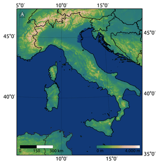
The experiment target domain spans from 35 to 48° N and from 5 to 20° E (Fig. 1). This area corresponds to the region where VHR-REA_IT CCLM data are available. The region includes a wide variety of topographically different sub-areas (mountainous areas such as the Alps and the Apennines and flat areas such as the Po Valley and coastal lines) which trigger local phenomena whose effects are challenging to identify for the downscaling models as they are not present in the low-resolution data.

Figure 1 Experimental domain with a 2 km digital elevation model.

3.4 Target variables and predictors

The target variables of the study are (i) 2 m temperature and (ii) horizontal wind components at 10 m: different, dedicated models to each target variable have been trained. The input ERA5 low-resolution data are both the target variables and the additional fields used as dynamical predictors to improve models' performance. The choice of the set of input fields was based on previous literature (e.g., Höhlein et al., 2020; Rampal et al., 2022; Harris et al., 2022) and on hardware constraints for the experiment. The selected fields used as predictor variables, for both target variables, are the following, corresponding to a total of 14 input channels to our networks:

• 2 m temperature;

• 10 m zonal and meridional wind speed;

• mean sea level pressure;

• sea surface temperature;

• snow depth;

• dew-point 2 m temperature;

• incoming surface solar radiation;

• temperature at 850 hPa;

• zonal, meridional and vertical wind speed at 850hPa;

• specific humidity at 850 hPa;

• total precipitation.

In addition, high-resolution static data have been fed to the models to guide the training and improve performance. These fields include

• digital elevation model (DEM),

• land cover categories,

• latitude.

DEM data consist of the Copernicus Digital Elevation Model (DEM; Copernicus, 2023) interpolated from a resolution of 90 m to a resolution of 2 km. Land cover data were retrieved from the Copernicus Global Land Service (Buchhorn et al., 2020) and interpolated from a resolution of 100 m to a resolution of 2 km. Given that land cover was utilized as a static variable in our analysis, we selected data from 2015: this year represents the earliest epoch available for the selected GLC dataset and falls approximately amid our experimental period of 2000–2020. Land cover class data have been converted to single-channel class masks for the DL models (totaling 16 channels). All static fields have been reprojected and aligned to the high-resolution 2 km EEA reference grid.

3.5 Dataset splitting strategy

The experimental database consists of hourly data from 2000 to 2020, totaling approximately 184 000 hourly samples for both low- and high-resolution data. The dataset was randomly divided into three subsets: 70 % for training (∼ 15 years, 128 873 samples), 15 % for validation (∼ 3 years, 27 616 samples), and 5 % for testing (∼ 1 year, 8760 samples). This random splitting ensures a uniform distribution of samples across years, months, and hours of the day in all three datasets. The testing dataset was limited to 1 year (5 % of the total dataset) to address time constraints associated with running all models during evaluation, particularly the diffusion model.

4 Methods

In this work, we test a deep generative latent diffusion model (LDM) for the downscaling task, conditioned with low-resolution predictors and high-resolution static data. The implemented LDM is trained to predict the residual error between a previously trained reference U-Net and the target variables; hence, the model is addressed as LDM_res (LDM_residual) hereafter. This residual approach has shown great performance in the application of pixel-space diffusion models (Mardani et al., 2023) and is tested here in the latent diffusion context. The underlying idea is to exploit the great ability of a relatively simple network (a U-Net) to properly capture the main, bigger-scale variability of the atmospheric high-resolution data and leverage the power of the generative diffusion model to only focus on the reconstruction of the smaller-scale, locally driven variability in the fields. Figure 2 shows the high-level flow chart of the training and inference setup for LDM_res, while Sect. 4.3 holds the detailed description of LDM_res architecture.

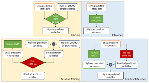
Figure 2 Training and inference flowcharts for the U-Net and GAN models (top row) and for LDM_res (bottom row). Differences between the non-residual and residual approaches are highlighted.

LDM_res is compared against three different baselines with increasing levels of complexity: the quadratic interpolation of ERA5, a U-Net, and a generative adversarial network (GAN). The implemented U-Net is the core base for each tested deep learning architecture. Indeed, the same reference U-Net network is used (i) as a baseline, (ii) as the generator of the implemented GAN, and (iii) for the calculation of the residual on which LDM_res is trained. With this approach, we aim to fairly compare the power of generating small-scale features of the adversarial and the diffusion methods.

A dedicated network has been trained for each model type for the two target variables: the 2 m temperature and 10 m horizontal wind components. The downscaling is performed for fixed time steps with an image-to-image approach.

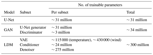
Given the incremental complexity of the tested models, in the following sections, we start by describing the core reference U-Net architecture (Sect. 4.1), then the GAN architecture (Sect. 4.2), and finally the LDM_res architecture (Sect. 4.3). Table 1 shows the number of trainable parameters for each model.

4.1 UNET

The core U-Net network implemented for our experiments is a standard U-Net architecture (Ronneberger et al., 2015), featuring an encoder (contracting path), a bottleneck, and a decoder (expansive path), with skip connections bridging corresponding levels between the encoder and decoder to preserve spatial information. To use a standard U-Net to perform downscaling, the input low-resolution data are interpolated with the nearest-neighbor interpolation to the target high resolution before feeding them to the network. Details on the U-Net architecture and training procedure are provided in Appendix A1 for conciseness.

4.2 GAN

The generative adversarial network (GAN) (Goodfellow et al., 2014, 2020) tested in this experiment consists of deep, fully convolutional generator and discriminator networks conditioned with low-resolution predictors and high-resolution static data. The generator is trained to output fields that cannot be distinguished from ground-truth images by a discriminator, which is trained on the other hand to detect the generator's “fake” outputs. Our reference GAN consists of a U-Net generator upgraded with a PatchGAN discriminator (Isola et al., 2017). The input data to the generator are low-resolution predictors and high-resolution static data only (no noise addition is performed), and we, therefore, obtain a deterministic GAN.

The generator architecture consists exactly of the U-Net described in Sect. 4.1. Details on the GAN architecture and training procedure are provided in Appendix A2 for conciseness.

4.3 Latent diffusion model

Diffusion models (Sohl-Dickstein et al., 2015) are probabilistic models meant to extrapolate a data distribution p(x) by corrupting the training data through the successive addition of Gaussian noise (fixed) and then learning to recover the data by reversing this noising process (generative).

The latent diffusion model (LDM) applied for this experiment is an architecture derived from stable diffusion (Rombach et al., 2021), specifically a re-adaptation of the conditional LDM LDCast (Leinonen et al., 2023), developed for precipitation nowcasting and already successfully applied for other variables (e.g., Carpentieri et al., 2023). The latent diffusion model derived for the downscaling task is composed of three main elements: a convolutional variational autoencoder (VAE), a conditioner, and a denoiser. The VAE is trained to project the residual high-resolution target variables to a latent space and to reconstruct them back to pixel space. In inference, only the decoder of the VAE is used to reproject the output from the other components of the model back to pixel space. The conditioner processes low-resolution predictors and high-resolution static data extracting relevant features for conditioning, embedding them into the denoiser. The denoiser is a U-Net-based network that manages the diffusion process in the latent space, refining data representations to reconstruct high-resolution outputs. It incorporates conditioning mechanisms to integrate context from low-resolution inputs and static data at multiple levels. Detailed descriptions of the individual components and their respective training configurations are provided, for conciseness, in Appendix A3. The total number of trainable parameters is shown in Table 1.

Table 1 Number of trainable parameters for each tested model.

5 Results

All the presented models were tested on a 1-year dataset, which was held out during the training and validation processes. The results from the LDM_res are evaluated based on a single inference run, obtained using 100 denoising steps; its potential to produce ensemble results is postponed to future analyses.

The following sections compare the results from LDM_res against the baselines using various verification metrics and distributions. In the Supplement, we report the comparison of results from the LDM trained with and without the residual approach to provide an overview of the improvements introduced by this method.

5.1 Qualitative evaluation

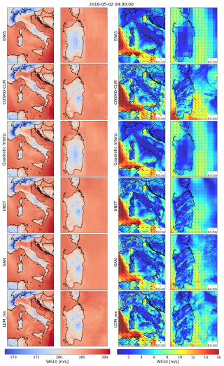
To provide a qualitative and perceptual overview of the obtained results, we present a random snapshot of downscaled variables compared with both the input ERA5 low-resolution data and the COSMO-CLM high-resolution reference truth (Fig. 3). The second and third columns show a zoom-in on Sardinia Island, providing a deeper overview of models' performance over complex terrain, coastal shores, and open sea. Both generative models, the GAN and LDM_res, effectively overcome the blurriness observed in both the quadratic interpolation and the U-Net for the target variables. Particularly for 2 m temperatures, LDM_res demonstrates a remarkable ability to identify and reconstruct discontinuities in the variable field (zoomed-in view in Fig. 3). Figure 3 also includes results for 10 m wind speed (in color), which is a derived field obtained by combining the two actual target variables of the models, U and V. Perceptually, the results for this variable from both GAN and LDM_res appear similar and equally plausible, displaying significantly more small-scale features compared to the U-Net. A deeper qualitative examination reveals that the GAN aligns well with the reference truth, particularly over land, but exhibits mode collapse over the sea for both target variables. An example of this effect is shown in the Supplement. Conversely, the LDM_res consistently generates plausible high-resolution data across the entire domain over both land and sea and for both target variables.

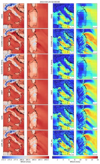
Figure 3 Downscaled variables from all the tested models against low-resolution ERA5 input data and high-resolution COSMO-CLM reference truth for a randomly picked timestamp. The left columns refer to 2 m temperature, and the right columns refer to 10 m wind speed. The second and fourth columns show a zoom-in on Sardinia Island.

5.2 Verification deterministic metrics

Figure 4 compares model results for different deterministic metrics, averaging results over the whole domain for each test time step. In addition to results from the baseline and tested models, Fig. 4 also reports results for the VAE of the LDM. These results are obtained using the VAE offline, feeding it with COSMO-CLM high-resolution data and calculating the metrics on the reconstructed data: this allows for the quantification of the LDM error resulting from the data decompression from the latent space only. We present three distance metrics, the root mean square error (RMSE), the mean bias (bias), and the coefficient of determination (R2), and one correlation metric, the Pearson correlation coefficient (PCC) (all calculated following Bell et al., 2021; see Appendix C for details).

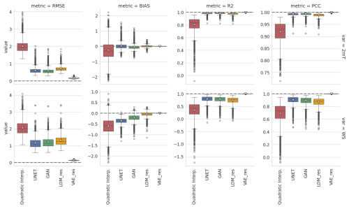
Figure 4 Comparison of deterministic metrics for spatially averaged results of the analyzed models (the top row refers to the 2 m temperature, and the bottom row refers to the 10 m wind speed). Notice that y axes are not shared between panels. The dashed line highlights the reference value for each metric, and the white triangle highlights the mean metric value.

The U-Net and GAN models show comparable and best results for all metrics, except for the bias. Indeed, minimizing the mean square error (MSE) is the exact goal of their training procedure. Conversely, the LDM has been trained on a much different objective but performs very well for all the metrics. As expected, all models struggle more in downscaling the wind components than the 2 m temperature. Biases show that all models perform very well, with LDM_res excelling, especially for temperature. The U-Net and the GAN models show spatially averaged biases within 1 °C for temperature, while LDM_res shrinks this variability to less than 0.5 °C. Spatially averaged biases amount to 1 m s⁻¹ for wind speed, with a narrower spread for LDM_res. The U-Net and LDM_res models show a less skewed distribution than the GAN model for the 2 m temperature: while the GAN model tends to underestimate the average 2 m temperature mostly, LDM_res shows a very balanced distribution for over- and underestimations. As for the wind speed biases, all the models always slightly underestimate the target variable.

The results show that the VAE contribution to LDM_res is the highest for the RMSE of 2 m temperature, while bias, R2, and PCC have little to no effect on temperature and wind speed.

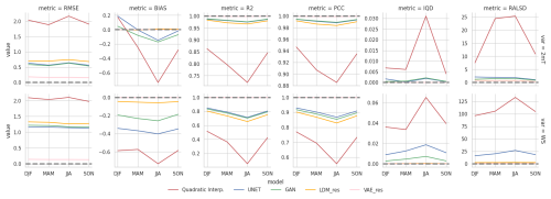
A more detailed evaluation of the models' performance using these metrics is provided in Fig. 5, where the test dataset is divided into meteorological seasons for seasonal analysis. The figure demonstrates that the results remain consistent across seasons, reinforcing the evaluations previously discussed. Notably, the summer season exhibits slightly lower metric values across all models. Additionally, deep learning models display more stable performance across different seasons than quadratic interpolation.

Figure 5 Comparison of different metrics/scores across seasons for the analyzed models (top row refers to the 2 m temperature and bottom row refers to the 10 m wind speed). Notice that y axes are not shared between panels. The dashed line highlights the reference value for each metric.

5.3 Spatial distribution of errors

The spatial distribution of averaged-in-time magnitude differences for both the target variables and all tested models is illustrated in Fig. 6. Within each panel, the numbers in squared brackets represent the 0.5 and 99.5 percentile values, offering insight into the highest errors recorded over the domain. Negative and positive values signify underestimation and overestimation, respectively, for both variables. Results from the quadratic interpolation of ERA5 data provide information on the original input data: 2 m temperature tends to be highly overestimated over complex terrain but underestimated on flat terrain, with smaller errors over sea. Wind speed, conversely, is largely underestimated over land, particularly over mountain ridges, with a tendency toward overestimation along coastal shores.

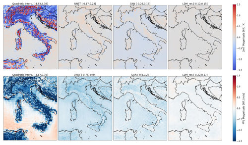
Figure 6 Spatial distribution of averaged-in-time magnitude difference for each tested model. The top row refers to the 2 m temperature, and the bottom row refers to the 10 m wind speed.

On the contrary, all DL-based models, including the U-Net baseline, exhibit substantially smaller errors. For 2 m temperature, errors remain below 0.3 °C, while for wind speed, they stay under 0.8 m s⁻¹ across the entire domain. Notably, the U-Net and GAN models perform comparably well for 2 m temperature, whereas LDM_res excels, leveraging diffusion processes to reduce the U-Net errors homogeneously.

As for the wind speed results, all models exhibit a tendency for underestimation. LDM_res demonstrates superior performance, minimizing errors to nearly zero over most of the domain, with a uniform distribution over land and sea. The GAN displays traces of its characteristic mode collapses, especially over the sea: this evidence indicates that these mode collapses persist statically in fixed locations over time consistently with the deployed training approach (i.e., feeding the network always across the entire, fixed domain).

5.4 Frequency distributions

Figure 7 presents the results in terms of frequency distributions. LDM_res precisely captures the reconstruction of the 2 m temperature frequency distribution, surpassing all other models. All DL models effectively mitigate the occurrence of cold extremes evident in the low-resolution data (as demonstrated by the quadratic interpolation distribution) while increasing the incidence of warm extremes. Notably, the adversarial training of the U-Net yields marginal enhancements in capturing the frequency distribution, with the GAN slightly outperforming the U-Net, particularly regarding cold extremes. Conversely, the diffusion process performed by LDM_res significantly corrects the U-Net residual errors, aligning closely with the reference-truth distribution across all temperature values.

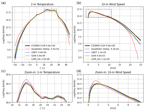
Figure 7 Comparison of frequency distributions for results from the tested models against COSMO-CLM reference truth. (a) and (c) refer to the 2 m temperature, and (b) and (d) refer to the 10 m wind speed. Counting of pixel-wise data is cumulated for the yearly test dataset over bins of 0.5 °C and 0.05 m s⁻¹ for temperature and wind speed, respectively. Notice that y axes are logarithmic to highlight the tails of the distributions, hence the extreme values. Panels (a) and (b) focus on the tails of the distributions, i.e., on extreme values, and panels (c) and (d) focus on the most frequent values and show a zoom-in on the dashed boxes for each variable. The legend also shows IQD values for each model.

Reconstructing the distribution of 10 m wind speed proves more challenging for all models, given the inherent chaotic nature of the U and V wind components compared to temperature, which is strongly influenced by terrain elevation. Nonetheless, performance outcomes mirror those of the 2 m temperature. The GAN modestly improves upon U-Net results, primarily in reducing occurrences of low wind speeds. LDM_res exhibits the highest performance in capturing both the tail and the center of the wind speed distribution.

These qualitative evaluations can be quantified by calculating a divergence score on the underlying empirical cumulative distribution function (CDF) of the data such as the integrated quadratic distance (IQD), as proposed by Thorarinsdottir et al. (2013) (see Appendix C for details). Values of the IQD score are indicated in Fig. 7. Consistently with the associated frequency distributions, values of IQD scores are lower for 2 m temperature compared to wind speed across all models. Notably, the LDM_res model achieves the best performance, with IQD scores 2 orders of magnitude lower than the U-Net and the GAN for 2 m temperature and 1 order of magnitude lower than the GAN for wind speed, highlighting its superior accuracy.

IQD scores were also computed for each season within the test dataset, with the results presented in Fig. 5. The models' scores align with the yearly analysis across all seasons. In particular, LDM_res exhibits the smallest score variations across seasons, indicating minimal sensitivity to seasonal changes.

5.5 Radially averaged power spectral density (RAPSD)

Figure 8 showcases the results in terms of radially averaged power spectral density (RAPSD) computed following the implementation outlined in Pulkkinen et al. (2019). The top row of the figure illustrates a single RAPSD, representing the average of each RAPSD calculated for every timestamp within the test dataset. To provide insight into the distribution of these values across all timestamps, the distributions of single-time RAPSD for fixed wavelengths are displayed in the bottom rows of Fig. 8. To provide a quantitative evaluation of the results in terms of power spectra, we calculated the log-spectral distance of the RAPSDs, referred to as the radially averaged log-spectral distance (RALSD) score, as proposed in Harris et al. (2022) (see Appendix C). For each model, values of the RALSD score are indicated in Fig. 8.

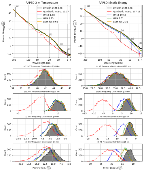
Figure 8 Comparison of radially averaged power spectral density (RAPSD) distributions for results from the tested models against COSMO-CLM reference truth. The left column refers to the 2 m temperature, and the right column refers to the 10 m wind speed. The first row shows the averaged-in-time spectra across the whole test dataset. Notice that in the first row y axes are logarithmic to highlight the tail of the distributions; hence the high frequencies. The bottom rows show the distributions of single-time RAPSD values for fixed wavelengths, namely, 269, 20, 9, and 5 km. The legend also shows RALSD score values for each model.

Overall, all DL models effectively reconstruct the 2 m temperature power spectra down to wavelengths of 10 km. However, LDM_res consistently outperforms both the U-Net and the GAN, as evident from panels (b) and (c) of Fig. 8 and the RALSD scores. The U-Net and the GAN yield similar results, with marginal yet consistent enhancements originating from the adversarial training of the U-Net, as also proven by the similar values of RALSD score. The diffusion process of LDM_res adeptly enhances the generation of small-scale features, showing precise reconstruction of the spectra to up to 9 km (see panel c). For scales smaller than 9–10 km, all models exhibit decreased performance, albeit still showing improvements over the quadratic interpolation of ERA5. LDM_res still outperforms the other models, but the very small scale variability of the original data is slightly underestimated. This behavior is to be ascribed to the VAE, as further elucidated in the Supplement. Indeed, original reference-truth data compressed and reconstructed by the VAE show the very same power spectra underestimation for scales smaller than 9 km. The loss of information is therefore due to and inherent to the projection to the latent space.

In contrast, results for wind speed distinctly demonstrate that generative models surpass both quadratic interpolation and U-Net, effectively matching the slope of the energy power spectra and remaining competitive with each other. Specifically, LDM_res consistently outperforms the GAN up to 7 km, as emphasized in panels (b) and (c) of Fig. 8 (right column). The RALSD scores for LDM_res and the GAN are comparable, with the GAN exhibiting a slightly lower value. This marginal improvement in the GAN is primarily attributed to enhanced performance at the smallest scales (below 4.2 km), where the model is more prone to generating artifacts. Similar to the 2 m temperature, for scales smaller than 10–9 km, both GAN and LDM_res experience reduced performance, although they consistently exhibit improvements over the U-Net. This behavior, for LDM_res, is in this case only partly to be ascribed to the VAE, as further shown in the Supplement, and an additional loss, for scales smaller than 9 km, is to be attributed intrinsically to the extraction of features with the diffusion process conditioned with the low-resolution data and high-resolution static data.

The RALSD scores were also computed for each season within the test dataset, with the results presented in Fig. 5. As for IQDs, the models’ RALSD scores align with the yearly analysis across all seasons. In particular, LDM_res exhibits the smallest score variations across seasons (together with the GAN for wind speed), indicating minimal performance sensitivity to seasonal changes.

5.6 Runtime performance

In this section, we compare the runtime performance of our tested models. These characteristics are of fundamental importance given the potential target applications of such models. Table 2 reports data for each model: to give a whole picture of the needed resources, we provide information on both the training and the inference requirements. The computational budgets reported for LDM_res include the time required for training and executing the U-Net, which generates the residual data, as well as the VAE_res. Consequently, the LDM_res budgets fully account for the total computational cost associated with training and running the entire modeling chain from scratch. Simulations were run on either NVIDIA GeForce RTX 4090 or NVIDIA A100 GPUs. The training dataset comprises 129 000 hourly samples over a target domain of 576 × 672 pixels (at high resolution) and 72 × 86 pixels (at low resolution). The U-Net and GAN training ran with a batch size of four for both target variables on the whole target domain. LDM_res training ran with batch sizes of eight and four for the two target variables (2 m temperature and 10 m wind components, respectively) on patches of 512 × 512 and 64 × 64 for high-resolution and low-resolution data, respectively. Inference times are calculated running with single-dimension batches across the entire domain.

Table 2 Number of GPU hours required for the training and inference (of a 1-year-long test set) by each tested model.

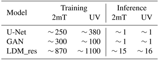
As shown in Table 2, LDM_res implies more expensive training and inference processes when compared with the tested DL baselines. This evidence is expected given the more complex structure of the diffusion model and its dimensions in terms of trainable parameters, which is an order of magnitude greater than that of the baselines. Nevertheless, the required computational time for both training and inference remains contained and competitive with the other available options. LDM_res requires 10 d over eight GPUs to train the models for both the target variables and 30 h on a single GPU to downscale 1 year of hourly temperature and wind data. In comparison, we note here that a 1-year-long COSMO-CLM simulation ran over the very same domain requires 61 h running on 2160 cores (Raffa et al., 2021) (of course producing many more high-resolution variables than the sole 2 m temperature and 10 m horizontal wind components).

6 Discussion

6.1 On the contribution of the VAE

In this section, we provide insights into the contribution of the VAE to the performance of LDM_res, thus showing the cost of moving to a latent space to perform the diffusion process. To do so, we compare results from LDM_res with VAE_res. VAE_res consists of the pure compression and decompression of the high-resolution data to and from the latent space and thus takes as input only the original reference-truth high-resolution target variables. On the contrary, LDM_res takes as input the low-resolution ERA5 predictors, high-resolution static data, and random noise; produces information in the latent space; and projects them in the pixel space using the VAE decoder. Both VAE_res and LDM_res also use the corresponding U-Net estimates for each target variable (i.e., the residual approach), but these quantities are subtracted before the encoding step (when applied) and added back after the decompression stage, acting essentially as constants. Therefore, the reconstruction errors for VAE_res are thus solely attributed to the compression/decompression processes, while the reconstruction errors for LDM_res arise from both the diffusion and decompression processes.

Figure 9 compares power spectra and the associated RALSD scores from the COSMO-CLM test reference-truth data with those from high-resolution test data generated using VAE_res and LDM_res. This figure highlights the decompression stage's contribution from the latent space to the pixel space in LDM_res.

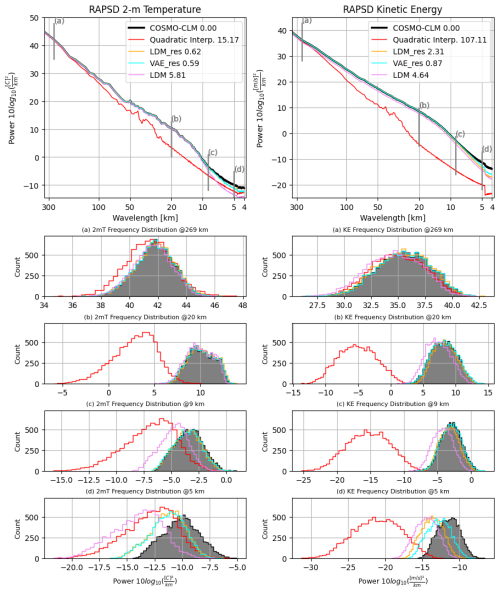
Figure 9 Comparison of radially averaged power spectral density (RAPSD) distributions for results from LDM_res, VAE_res, and LDM against COSMO-CLM reference truth and ERA5 quadratic interpolation. The left column refers to the 2 m temperature, and the right column refers to the 10 m horizontal wind speed. The first row shows the averaged-in-time spectra across the whole test dataset. Notice that in the first row y axes are logarithmic to highlight the tail of the distributions; hence the high frequencies. The bottom rows show the distributions of single-time RAPSD values for fixed wavelengths, namely, 269, 20, 9, and 5 km. The legend also shows RALSD score values for each model.

For 2 m temperature, the power spectra from the LDM_res and VAE_res are nearly identical across all wavelengths, including the smallest scales, with values of RALSD of 0.62 and 0.59, respectively. This indicates that the errors in reconstructing COSMO-CLM spectra with LDM_res are attributable solely to the decompression stage, with the diffusion process effectively and accurately extracting latent features from the conditional data. On the contrary, for 10 m wind speed, a more chaotic field, discrepancies between the power spectra from LDM_res and VAE_res are observed at scales smaller than approximately 7 km, with values of RALSD of 2.31 and 0.87, respectively. These differences highlight the errors introduced by the sole extraction of features by the diffusion process.

It is worth noting that these reconstruction errors occur at spatial scales smaller than the considered effective resolution of the reference numerical simulation. The effective resolution is indeed coarser than the nominal spatial resolution, estimated to be approximately 6×Δx (i.e., ∼ 13 km in this study), as indicated by Skamarock et al. (2014), or within the range of 4×Δx to 8×Δx, as reported by Abdalla et al. (2013), for example.

6.2 On the contribution of the residual approach

In this section, we compare the performance of the LDM trained with and without the residual approach, highlighting the significant improvements introduced by the residual methodology. The comparison focuses on the frequency distribution and the radially averaged power spectral density (RAPSD), as shown in Figs. 10 and 9, respectively, along with their associated metrics, IQD and RALSD.

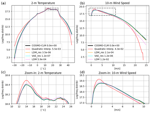
Figure 10 Comparison of frequency distributions for results from LDM_res, VAE_res, and LDM against COSMO-CLM reference truth and ERA5 quadratic interpolation. Panels (a) and (c) refer to the 2 m temperature, and panels (b) and (d) refer to the 10 m wind speed. Counting of pixel-wise data is cumulated for the yearly test dataset over bins of 0.5 °C and 0.05 m s⁻¹ for temperature and wind speed, respectively. Notice that y axes are logarithmic to highlight the tails of the distributions; hence the extreme values. The top row focuses on the tails of the distributions, i.e., on extreme values, and the bottom row focuses on the most frequent values and shows a zoom-in on the dashed boxes for each variable. The legend also shows IQD values for each model.

The analysis reveals notable differences between the two models, particularly in (i) accurately estimating the most frequent values of 2 m temperature; (ii) reconstructing the full frequency distribution of wind speed; (iii) reconstructing the 2 m temperature power spectra at small scales, where the non-residual LDM underperforms compared to the quadratic interpolation of ERA5; and (iv) reconstructing the 10 m wind speed power spectra across all scales, with the non-residual LDM exhibiting a quasi-constant lag across all wavelengths.

The corresponding VAEs for the two models (VAE and VAE_res) show comparable performance except at the smallest scales of the 2 m temperature power spectra (not shown). Consequently, the diminished performance of the non-residual LDM can be attributed to the VAE only in this specific case (iii). All other deficiencies are solely due to the diffusion process. Training the diffusion model to reconstruct a residual field instead of the original target field significantly enhances performance, improving the reconstruction of frequency distributions and power spectra across all wavelengths, particularly for chaotic variables such as wind speed.

6.3 On the reconstruction of extreme events: a case study of strong winds

To evaluate the performance of the deep learning models in a challenging scenario, we selected 7 February 2022 as a case study. This analysis represents a preliminary investigation of the deep learning models' ability to reconstruct a single strong wind event and their performance in reproducing time series when applied to consecutive time steps. The selected event provides independent data separate from the training, validation, and test datasets previously discussed. The date 7 February 2022 is particularly noteworthy due to widespread strong winds across Italy prompting weather alerts in various regions and causing significant wind-related damage. On this day, the Italian peninsula was affected by a pronounced pressure gradient resulting from the southward descent of a low trough from northeastern Europe toward the Ionian Sea and the simultaneous presence of a high-pressure system centered over the Bay of Biscay (see Fig. 11). This synoptic configuration generated widespread föhn conditions, with strong northerly to northwesterly winds affecting northern regions and areas downwind of the Apennine ridges.

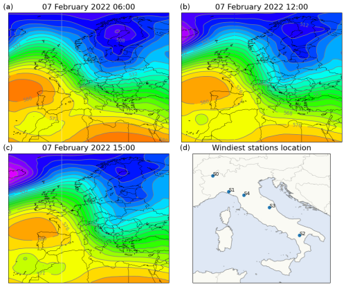
Figure 11 Panels (a), (b), and (c) show the evolution of geopotential height at 500 hPa [dam] from 06:00 UTC on 7 February 2022, to 15:00 UTC on 7 February 2022 (ERA5 data). (d) shows the location of five weather stations used for the analysis.

The performance of the models was assessed at five locations of interest corresponding to Italian weather stations that recorded hourly wind speeds exceeding 20 m s⁻¹ during the case study. These stations, situated in complex terrain, are highlighted in the final panel of Fig. 11. Figure 12 presents the time series of 10 m wind components and wind speeds at each target location. For 10 m wind speed, observational data collected by the weather stations are included as a reference for comparison.

As illustrated in Fig. 12, significant differences are observed between ERA5 and COSMO-CLM data across all reference stations. The dynamical downscaling approach of COSMO-CLM produces substantially higher wind speeds compared to the low-resolution ERA5 data, with discrepancies reaching up to 10–13 m s⁻¹. While COSMO-CLM still underestimates wind speeds compared to observations, its temporal evolution of wind flux generally aligns well with measurements.

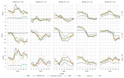
Figure 12 Hourly evolution of 10 m wind components and 10 m wind speed as reconstructed by all models on 7 February 2022 in the selected target locations. Available 10 m wind speed observations from each weather station are also reported.

The deep learning models demonstrate remarkable performance, with the target ground truth being the COSMO-CLM output. All three models effectively reconstruct wind intensities for both components, showing minimal dependency on the underestimation present in the input low-resolution data. Notably, the models accurately capture the temporal evolution of wind components, frequently correcting the phase discrepancies in wind speed trends (increases or decreases) present in the low-resolution data. This capability is particularly noteworthy given that the models are trained exclusively for image-to-image downscaling without access to temporal information from adjacent time steps. Among the deep learning models, results are generally comparable. However, the GAN and U-Net models tend to produce smoother temporal signals compared to the LDM_res model and the COSMO-CLM baseline.

7 Conclusions

This study compares the performance of various downscaling models, focusing on their ability to reconstruct high-resolution meteorological variables from low-resolution input data. The models evaluated include a baseline U-Net, a generative adversarial network (GAN), and a latent diffusion model with a residual approach against the reference U-Net (LDM_res). The results are analyzed using qualitative evaluations, deterministic metrics, spatial error distributions, frequency distributions, radially averaged power spectral density (RAPSD), and runtime performance.

LDM_res demonstrates superior performance across most metrics, particularly in reconstructing fine-scale details and maintaining accuracy in frequency distributions (especially for the extreme values) and spatial error distributions. LDM_res outperforms the other models in reconstructing the power spectra, showing superior performance, especially for wind speed, with outstanding results for wavelengths of up to 7 km. Residual errors at smaller scales can be attributed to the data projection into the latent space, specifically to the usage of the VAE. This performance loss might be mitigated by conducting the diffusion process directly in the pixel space. However, this alternative approach would substantially increase the computational costs for both training and inference.

The remarkable results of LDM_res are to be ascribed equally to two fundamental aspects of the proposed model:

• the incomparable effectiveness of the diffusion process in extracting features and leveraging the provided conditioning;

• the residual approach which allows the diffusion process to focus only on smaller scales and more subtle characteristics of the fields, delegating the estimates of large-scale variation in the atmospheric fields to a simpler, yet effective, network.

However, the great performance of LDM_res comes at the cost of significantly higher computational requirements for both training and inference when compared to the other DL models, i.e., the U-Net or the GAN. Nonetheless, LDM_res still offers a significant advantage in terms of inference speed and computational efficiency once the model is trained when compared to the extensive computational resources required by COSMO-CLM.

In conclusion, the ability of LDM_res to accurately reproduce the statistics of the COSMO-CLM model reference-truth data, provided with the same input, demonstrates its potential as an effective and versatile dynamical downscaling emulator. This approach significantly accelerates the downscaling process compared to traditional numerical dynamical models, making it highly suitable for a broad range of important applications, such as downscaling seasonal forecasts or climate projections.

Nevertheless, two primary limitations remain in the proposed deep learning approach: (i) inter-variable consistency and (ii) temporal consistency of the generated fields. These fundamental aspects, which are inherently preserved in dynamical downscaling performed using physically based numerical models, are not guaranteed by the design of this study. Specifically, LDM_res is applied and trained separately for 2 m temperature and 10 m horizontal wind components, performing image-to-image downscaling. Regarding inter-variable consistency, results from this study, as well as findings from other works, such as Mardani et al. (2023), suggest that a multi-variable approach is feasible and could provide significant benefits by better leveraging all available parameters within the network. Concerning temporal consistency, although results briefly showcased in the presented case study indicate that the DL model generates consecutive time steps that form rather consistent time series, further investigation and testing are necessary to thoroughly address this aspect, as discussed in the “Future work” section.

8 Future work

The results presented in this work suggest several promising directions for further investigation into the application of latent diffusion models for downscaling.

Addressing the primary limitations of our DL approach, namely, (i) inter-variable consistency and (ii) temporal consistency of the generated fields, is a key priority. Applying LDM_res with a multi-variable approach requires no architectural adjustments and could yield valuable insights, such as whether additional variables necessitate larger network architectures to optimize performance. The potential and efficiency of a multi-variable approach have already been demonstrated in pixel-space diffusion downscaling by Mardani et al. (2023). Further evaluation of the temporal consistency of downscaled data in this version of LDM_res is also relevant. Enhancements in this area could involve conditioning the diffusion process on a (short) temporal sequence of low-resolution fields or incorporating previous high-resolution outputs in an auto-regressive approach. Additionally, the generative capabilities of LDM_res need to be explored to assess the potential added value of a DL-generated ensemble.

Future developments could explore the integration of latent diffusion models into existing modeling frameworks and operational systems, such as using them as postprocessing tools for real-time weather forecasts, seasonal forecasts, and climate projections. These integrations would require tailored training procedures, alignment with operational inputs and reference data, and rigorous validation to ensure robustness and compatibility with practical applications. For example, ongoing research, funded as an innovation project within this research's funding, is already investigating the effectiveness of LDM_res in downscaling precipitation and temperature, in a multi-variable approach, from climate projections predictors. This exploration is expected to further elucidate the versatility and robustness of the proposed approach and showcase its practical applications.

Appendix A: Architecture and training procedure of the DL models

A1 UNET

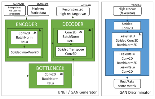
The U-Net encoder is composed of four blocks, each consisting of a layer containing two consecutive 2D convolutions with rectified linear unit (ReLU) activation interspersed with batch normalization to ensure stable learning (Ioffe and Szegedy, 2015), and a max-pooling operation. The max-pooling layer reduces the spatial resolution by half, enabling the model to capture increasingly complex features while reducing the image dimensions. The output of each encoder block is used in both the next encoder block and the corresponding decoder block through skip connections. The decoder mirrors the encoder with transposed 2D convolutional layers and upsampling steps to go back to the starting resolution. The use of batch normalization ensures robust learning, while the skip connections help preserve critical spatial information across the encoder–decoder bridge. The total number of trainable parameters for the U-Net is ∼ 31 M (Table 1). Details on the U-Net structure and resolutions are depicted in Fig. A1.

The loss function used for training is the mean squared error (MSE) loss with mean reduction, which is suitable for regression-based tasks and ensures smooth convergence. The Adam optimizer (Kingma and Ba, 2015), chosen for its effectiveness in handling non-stationary objectives and sparse gradients, is employed with a learning rate of 10⁻³ and no weight decay. Training is conducted for up to 100 epochs, with early stopping enabled to terminate training if validation performance does not improve over 10 consecutive epochs. Each epoch involved iterating through the dataset with a batch size of 16, which was chosen to balance memory constraints and training efficiency. The network is constantly fed with the whole target domain, and no patch training is applied.

Figure A1 Details on the architectures for the reference U-Net and the GAN implemented for the downscaling task. The reference U-Net and the generator networks are depicted on the left panel, and the discriminator network is on the right panel. NN stands for nearest neighbor.

A2 GAN

The discriminator of the GAN is a PatchGAN convolutional classifier (Isola et al., 2017), which focuses on structures at the scale of image patches. The structure of the discriminator is composed of modules of the form convolution–batch norm–ReLU. It assigns a “realness” score to each N×N patch of the image, runs convolutionally across the image, and allows us to obtain an overall score by averaging all responses for each patch. High-quality results can be obtained with patches much smaller than the full size of the image, with relevant advantages in terms of resources for the training and application to arbitrarily large images. Details on the discriminator network structure and resolutions are depicted in Fig. A1. The total number of trainable parameters for the GAN is ∼ 34 M (Table 1).

The training procedure follows the combined loss function approach for GANs (Goodfellow et al., 2020), including recent improvements to promote stability in the training (Esser et al., 2021), with the primary goal of balancing the minimization of both the generator's and the discriminator's losses, which are adversarial. The hyperparameters set for the training are derived from the search and optimization already performed by Esser et al. (2021), while the parameters we manually fine-tuned are described in the following. The pixel loss we used is the mean absolute error (MAE), while the discriminator loss is the hinge loss. The discriminator is activated after 50 000 training steps, giving the generator time to learn to generate consistent outputs and thus stabilizing the adversarial training (Esser et al., 2021). After activating the discriminator, the network is trained by updating alternatively the gradients of the generator and the discriminator. The network is constantly fed with the whole target domain and no patch training is applied. The Adam optimizer (Kingma and Ba, 2015) is used for both the generator and the discriminator, with a base learning rate equal to $\mathrm{4.5}\times {\mathrm{10}}^{-\mathrm{6}}$ multiplied by the number of the GPU and the batch size used for the training – i.e., $\mathrm{4.5}\times {\mathrm{10}}^{-\mathrm{6}}\times$ 1 GPU × 4 (batch size) (Goyal et al., 2018), and with beta parameters set to 0.5 and 0.9. Training is conducted for up to 100 epochs, with early stopping enabled to terminate training if validation performance does not improve over 10 consecutive epochs. Each epoch involved iterating through the dataset with a batch size of four chosen to balance memory constraints and training efficiency.

A3 LDM_res

The latent diffusion model derived for the downscaling task is composed of three main elements: a convolutional variational autoencoder (VAE), a conditioner, and a denoiser. In the following sections, we report a detailed description of each model component and its training procedure. Figures A2 and A3 summarize the training and inference procedures for the model and the main structure of each component architecture, respectively.

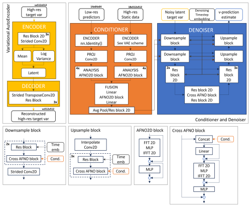
Figure A2 An overview of the components of our downscaling latent diffusion model: the variational autoencoder, the conditioner, and the denoiser networks. Conv denotes convolution. The MLP (multilayer perceptron) is a block consisting of a linear layer, activation function, and another linear layer. Res block denotes a ResNet-type residual block. The v in the array size labels stands for the number of target variables (1 for 2 m temperature and 2 for 10 m horizontal wind speed components).

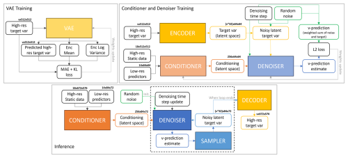
Figure A3 An overview of the training and inference procedures for our downscaling latent diffusion model. The v in the array size labels stands for the number of target variables (1 for 2 m temperature and 2 for 10 m horizontal wind speed components).

A3.1 Variational autoencoder

The variational autoencoder (VAE) projects the residual high-resolution data from the pixel space to a continuous latent space (encoder) and projects them back to the pixel space (decoder). We train a dedicated VAE for the 2 m temperature and a dedicated VAE for the 10 m wind speed components independently from the conditioner and denoiser. Once trained, the VAE weights are kept constant during the training of the rest of the network architecture. During inference, only the decoder of the VAE is used (see Fig. A3).

The encoder and the decoder are structured as 2D convolutional networks composed of blocks of a ResNet residual block (Stephan et al., 2008) and a downsampling/upsampling convolutional layer. Three levels of such blocks are used, each reducing each spatial dimension by a factor of 2, while the number of channels is bottlenecked at 32 times the number of input target variables (i.e., 32 × 1 for the 2 m temperature and 32 × 2 for the 10 m wind speed components). The VAE bottleneck latent space is regularized with a loss based on Kullback–Leibler (KL) divergence (Kullback and Leibler, 1951; Csiszar, 1975) between the latent variable and a multivariate standard normal variable.

The VAEs are trained on random 512 × 512 pixel patches of high-resolution target variables, with a batch size of 16. The training process for the VAEs leverages AdamW optimizer (Loshchilov and Hutter, 2019), with a base learning rate of 1×10⁻³, the beta parameters set to 0.5 and 0.9, and a weight decay of 1×10⁻³. The loss function combines a reconstruction loss, computed as the mean absolute error (MAE) between predicted and target outputs, with the KL divergence term. The KL divergence, scaled by a weight factor (λ_KL=0.01), enforces a standard normal distribution on the latent space. A ReduceLROnPlateau scheduler (PyTorch, 2023) is employed to dynamically adjust the learning rate by reducing it by a factor of 0.25 if the validation reconstruction loss does not improve for three consecutive epochs. Training is conducted for up to 100 epochs, with early stopping enabled to terminate training if validation performance does not improve over 10 consecutive epochs.

While the space dimensions are reduced by a factor of 8² (from 512 × 512 to 64 × 64 pixel patches), the number of channels is increased from 1 (for the 2 m temperature) and 2 (for the 10 m wind speed components) to 32 and 64, respectively: the overall amount of data is therefore compressed only by a factor of 2 for both VAEs (from 1 × 512 × 512 to 32 × 64 × 64 and from 2 × 512 × 512 to 64 × 64 × 64). Nevertheless, the gain in training performance of the denoiser and conditioner is much greater than the data reduction factor as the compression along the space dimension is more relevant for reducing the computational cost of the training than the increase in channel number (Rombach et al., 2021).

Figure A2 depicts details of the VAE's structure.

A3.2 Conditioner

The conditioner stack acts as a context encoder to process the low-resolution predictors and high-resolution static data and embed them into each level of the denoiser U-Net architecture. Initially, both datasets are preprocessed by passing through a dedicated encoder, a projection layer, and an analysis sequence before being merged. The predictors' encoder is a basic identity layer since they already have the same spatial dimensions as the latent space (64 × 64). The static data encoder is a variational encoder with the same structure as the VAE described in the previous section, Sect. A3.1. For both datasets, the projection layer is a 2D convolutional layer with a unitary kernel size used to increase the number of channels, and the analysis is a sequence of four 2D adaptive Fourier neural operator (AFNO) blocks (following Pathak et al., 2022), used to extract relevant features. After preprocessing, the conditioning information is prepared to be fed to each level of the denoiser U-Net by applying a combination of average pooling and 2D ResNet layers. Figure A2 depicts details of the conditioner's structure.

A3.3 Denoiser

Our denoising stack is structured as the one of LDCast (Leinonen et al., 2023), a re-adaptation of the U-Net-type network applied in the original latent diffusion model (Rombach et al., 2021). The resulting denoiser network consists of a U-Net backbone enabled with a conditioning mechanism based on 2D AFNO blocks (Leinonen et al., 2023), aiming at a cross-attention-like operation (as suggested in Guibas et al., 2022). This structure is meant to control the high-resolution synthesis process feeding the conditioning in each level of the U-Net architecture.

For the downscaling task, the conditioning information consists of the low-resolution predictors' data and the high-resolution static data elaborated by the conditioner. Figure A2 depicts the details of the denoiser's structure.

To improve the reconstruction of extreme values (for both temperature and wind speed), we implemented the v-prediction parameterization in our LDM model, following Salimans and Ho (2022): this parameterization trains the denoiser to model a weighted combination of both the noise and the start image, instead of either the only noise or the only start image as done in the more traditional implementations eps and x0, respectively.

As shown in Fig. A3, the conditioner and the denoiser are trained together, minimizing the mean square error (MSE), feeding the network with random patches of ERA5 predictors (64 × 64 pixels) and static data (512 × 512 pixels) for the conditioning and high-resolution target variables (512 × 512 pixels) for the ground truth. The batch size is set to four and eight for the 2 m temperature and 10 m wind components models, respectively, tuned to balance memory constraints and training efficiency. The training is performed using the AdamW optimizer (Loshchilov and Hutter, 2019), with a base learning rate of 1×10⁻⁴, the beta parameters set to 0.5 and 0.9, and a weight decay of 1×10⁻³. A ReduceLROnPlateau scheduler (PyTorch, 2023) is employed to dynamically adjust the learning rate by reducing it by a factor of 0.25 if the validation loss does not improve for three consecutive epochs. Additionally, exponential moving averaging (EMA) is applied to the network weights, following Rombach et al. (2021). Training is conducted for up to 100 epochs, with early stopping enabled to terminate training if validation performance does not improve over 10 consecutive epochs. The other hyperparameters set for the training are derived from the implementation of the LDCast model by Leinonen et al. (2023).

Appendix B: Additional snapshots of downscaled data

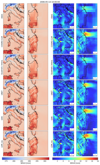
Some additional snapshots of downscaled data from all the tested models are shown in Figs. B1 and B2. The left columns refer to 2 m temperature, and the right columns refer to 10 m wind speed. The second and fourth columns show a zoom-in on Sardinia Island.

Figure B1 Downscaled variables from all the tested models against low-resolution ERA5 input data and high-resolution COSMO-CLM reference truth for an additional random timestamp.

Figure B2 Downscaled variables from all the tested models against low-resolution ERA5 input data and high-resolution COSMO-CLM reference truth for an additional random timestamp.

Appendix C: Calculation of verification metrics

In Sect. 5.2, we discuss the following metrics: three distance metrics; the root mean square error (RMSE); the mean bias (bias); the coefficient of determination (R2); and one correlation metric, the Pearson correlation coefficient (PCC). All the metrics are calculated with the xskillscore library (Bell et al., 2021). Definitions are as follows:

$$\begin{array}{}\text{(C1)}& {\displaystyle }\mathrm{RMSE}=\sqrt{{\displaystyle \frac{\mathrm{1}}{n}}\sum _{i=\mathrm{1}}^n(a_i-b_i{)}^{\mathrm{2}}},\text{(C2)}& {\displaystyle }\mathrm{bias}={\displaystyle \frac{\mathrm{1}}{n}}\sum _{i=\mathrm{1}}^n(a_i-b_i),\text{(C3)}& {\displaystyle }{\mathrm{SS}}_{\mathrm{tot}}=\sum _{i=\mathrm{1}}^n(a_i-\stackrel{\mathrm{‾}}{a}{)}^{\mathrm{2}},\text{(C4)}& {\displaystyle }{\mathrm{SS}}_{\mathrm{res}}=\sum _{i=\mathrm{1}}^n(a_i-b_i{)}^{\mathrm{2}},\text{(C5)}& {\displaystyle }{R}^{\mathrm{2}}=\mathrm{1}-{\displaystyle \frac{{\mathrm{SS}}_{\mathrm{res}}}{{\mathrm{SS}}_{\mathrm{tot}}}},\text{(C6)}& {\displaystyle }\mathrm{PCC}={\displaystyle \frac{{\sum }_{i=\mathrm{1}}^n(a_i-\stackrel{\mathrm{‾}}{a})(b_i-\stackrel{\mathrm{‾}}{b})}{\sqrt{{\sum }_{i=\mathrm{1}}^n(a_i-\stackrel{\mathrm{‾}}{a}{)}^{\mathrm{2}}}\sqrt{{\sum }_{i=\mathrm{1}}^n(b_i-\stackrel{\mathrm{‾}}{b}{)}^{\mathrm{2}}}}},\end{array}$$

where a and b are the predicted and reference-truth values, respectively, for every ith pixel of the domain and n is the total number of pixels in the domain.

In Sect. 5.4, we discuss the integrated quadratic distance score, which is calculated following Thorarinsdottir et al. (2013) and measures the similarity between two distributions by the integral over the squared difference between the two distribution functions:

$$\begin{array}{}\text{(C7)}& \mathrm{IQD}=\underset{\min }{\overset{\max }{\int }}\left(F\right(t)-G(t){)}^{\mathrm{2}}\mathrm{d}t,\end{array}$$

where F(t) and G(t) are the empirical cumulative distribution function of the modeled and reference-truth data, respectively, computed following the implementation outlined in Pulkkinen et al. (2019); the minimum and maximum are [−30, 45] °C and [0, 25] m s⁻¹ for 2 m temperature and wind speed, respectively; dt has been fixed to 0.5 °C and 0.25 m s⁻¹ for 2 m temperature and wind speed, respectively.

In Sect. 5.5, we discuss results in terms of the log-spectral distance of the RAPSDs, referred to as the radially averaged log-spectral distance (RALSD) score, following Harris et al. (2022):

$$\begin{array}{}\text{(C8)}& \mathrm{RALSD}\mathit{\_}\mathrm{score}=\sqrt{{\displaystyle \frac{\mathrm{1}}{N}}\sum _{i=\mathrm{1}}^N{\left(\mathrm{10}{\log }_{\mathrm{10}}{\displaystyle \frac{{\stackrel{\mathrm{‾}}{P}}_{\mathrm{true}}}{{\stackrel{\mathrm{‾}}{P}}_{\mathrm{gen}}}}\right)}^{\mathrm{2}}},\end{array}$$

where ${\stackrel{\mathrm{‾}}{P}}_{\mathrm{true}}$ and ${\stackrel{\mathrm{‾}}{P}}_{\mathrm{gen}}$ are the radially averaged power spectral densities of the reference-truth and modeled data, respectively, computed following the implementation outlined in Pulkkinen et al. (2019), and N is the number of frequencies (i.e., 336).