Development of a fast radiative transfer model for ground-based microwave radiometers (ARMS-gb v1.0): validation and comparison to RTTOV-gb

This study proposes a fast radiative transfer model, the Advanced Radiative Transfer Modeling System – ground-based (ARMS-gb), designed to simulate brightness temperatures observed by ground-based microwave radiometers. ARMS-gb employs a clear-sky radiative transfer solver to account for atmospheric thermal emissions, while gaseous absorption is estimated using a statistical regression scheme. To enhance simulation accuracy, particularly in moist environments, seven humid profiles from the University of Maryland, Baltimore County 48-profile dataset are added to the European Centre for Medium-Range Weather Forecasts 83-profile dataset to train the gaseous absorption scheme. Additionally, an advanced water vapor vertical interpolation method is incorporated, offering improved accuracy compared to the interpolation method used in Radiative Transfer for TOVS (RTTOV)-gb. The standard deviation is reduced by 0.15 K in channels with strong water vapor absorption. The Jacobians calculated by these two interpolation modes are also different. To further validate ARMS-gb's performance, simulations using both ARMS-gb and RTTOV-gb are compared against real observations from two ground-based microwave radiometers. The observation minus background analyses demonstrates that ARMS-gb aligns well with RTTOV-gb and achieves smaller standard deviations under high-humidity conditions. Furthermore, the capability of ARMS-gb to monitor the observational quality of ground-based microwave radiometers is demonstrated.

1 Introduction

Ground-based microwave radiometers (GMRs) are considered vital tools in meteorological research due to their ability to provide continuous, high-temporal-resolution observations of atmospheric thermodynamical variables (Cimini et al., 2006; Wei et al., 2021). These instruments can operate under all-sky conditions, making them particularly useful for monitoring rapid changes within the planetary boundary layer (PBL). The PBL, which may extend from the surface to a few kilometers above, is a critical region where exchanges of heat, moisture, and momentum between the ground and the atmosphere predominantly occur (Wu et al., 2024). Observations from GMRs offer a unique advantage for understanding PBL dynamics, providing valuable insights into processes such as convection, turbulence, and boundary layer transitions (De Angelis et al., 2017).

The assimilation of GMR observations into numerical weather prediction (NWP) models holds significant potential for enhancing forecast accuracy, particularly in the lower atmosphere. Current NWP models often face substantial uncertainties near the ground surface due to both observational gaps and the complex physical processes within the PBL. By incorporating GMR observations, temperature and humidity in the PBL can be characterized more accurately, leading to improved initial conditions for NWP models (Illingworth et al., 2019; Leuenberger et al., 2020). Consequently, temperature and humidity profiles retrieved from GMR observations have been assimilated into NWPs in previous studies (e.g., Caumont et al., 2016; Martinet et al., 2020). These studies show that such indirect assimilations enhance the accuracy of forecasts involving temperature inversions and humidity gradients, which are crucial for predicting fog and the initiation of convection. However, the performance of these assimilations is often limited by challenges in estimating biases in GMR observations (Lin et al., 2023). This limitation can be mitigated by directly assimilating the observed brightness temperatures (BTs) from GMRs. It has been demonstrated that directly assimilating BTs from two channels has a positive impact on forecasting temperature and humidity in the PBL (Vural et al., 2024). The advantage of direct assimilation of GMR observations is further highlighted when compared to indirect assimilation results in forecasting extreme precipitation events (Cao et al., 2023). Radiative transfer models (RTMs) are essential in direct data assimilation, as they map atmospheric parameters from NWP models onto satellite or GMR observations. Numerous fast RTMs have been developed for the direct assimilation of satellite observations, such as the Radiative Transfer for TOVS (RTTOV) (Saunders et al., 2018; Hocking et al., 2021), the Community Radiative Transfer Model (CRTM) (Weng and Liu, 2003; Stegmann et al., 2022; Karpowicz et al., 2022), and the Advanced Radiative Transfer Modeling System (ARMS) (Weng et al., 2020; Yang et al., 2020). For use with GMRs, few RTMs are specifically designed for this purpose, with RTTOV-ground based (RTTOV-gb) (De Angelis et al., 2016; Cimini et al., 2019) being a notable exception. Unlike the traditional RTTOV, RTTOV-gb is optimized to handle the unique geometries and atmospheric paths associated with GMRs. While the coefficients for RTTOV are trained using AMSUTRAN (Turner et al., 2019), the coefficients for RTTOV-gb are trained using an updated version of the Millimeter-wave Propagation Model, as detailed by Rosenkranz (1998) (hereafter referred to as R98). A further updated version of R98 is introduced by Rosenkranz (2017) (hereafter referred to as R17), and its uncertainties are analyzed by Cimini et al. (2018). RTTOV-gb v1.0 now supports coefficients trained using both R98 and R17.

In addition to AMSUTRAN, R98, and R17, the Monochromatic Radiative Transfer Model (MonoRTM) can also provide line-by-line (LBL) results of radiance and transmittance, and its accuracy in simulating upwelling radiative transfer (RT) has been evaluated against AMSUTRAN (Cady-Pereira et al., 2021). On the other hand, for downwelling RT simulations, BTs produced by different types of LBL models can vary significantly. A study comparing results from five different LBL models found discrepancies as large as 1.5 K in channel 1 of the MP-3000A (Yang and Min, 2018), underscoring the importance of using a reliable and accurate LBL model to train fast RTMs for optimal performance. However, there are few studies that provide intercomparisons between fast RTMs trained with different microwave LBL models in downwelling RT simulations.

Furthermore, due to the use of terrain-following coordinates, the pressure levels in NWP models are not fixed, necessitating vertical interpolation in both RTTOV and RTTOV-gb. Hocking (2014) compared five vertical interpolation methods within RTTOV, finding that the choice of interpolation mode affects not only the simulated BTs but also the Jacobian calculations. Kan et al. (2024) proposed an advanced water vapor interpolation method, significantly reducing biases caused by vertical interpolation in water vapor absorption channels of microwave sensors on board satellites. It is important to evaluate the differences in forward simulations and Jacobians caused by vertical interpolation modes from the perspective of GMR applications.

In this study, a new RTM (ARMS-gb) capable of simulating BTs observed by GMRs and their Jacobian is proposed. ARMS-gb relies on a clear-sky RT solver and employs MonoRTM to train the gaseous absorption scheme. The accuracy of ARMS-gb in a moist environment is improved by enriching the training dataset and incorporating the advanced interpolation mode proposed by Kan et al. (2024). This development also marks the first intercomparison between two fast RTMs for GMRs. In the following section, each component of ARMS-gb is described in detail, including the clear-sky radiative transfer (RT) solver, the gaseous absorption scheme, and the Jacobian calculation module. Section 3 investigates the accuracy of ARMS-gb by comparing its results with those of MonoRTM. The improvements in accuracy achieved by enriching the training dataset are evaluated, and the impact of vertical interpolation on both forward simulations and Jacobian calculations is analyzed. In Sect. 4, ARMS-gb and RTTOV-gb are used to simulate real observations from two GMRs under different climate conditions. Observation minus background (OMB) analyses from the two RTMs are compared. Additionally, the capability of ARMS-gb to monitor the observational quality of GMRs is demonstrated. A summary of the findings is provided in Sect. 5.

2 Model development

The primary objective of this study is to develop ARMS-gb capable of simulating BTs observed by GMRs. These BTs are directly linked to downwelling radiances at the surface. Currently, ARMS-gb is limited to simulations under clear-sky conditions; however, a particle scattering module will be integrated in the near future to extend its capabilities and enable simulations under all-sky conditions.

2.1 Clear-sky RT equation

Without considering scattering effects, the RT equation (Liou, 1992) simplifies to

$$\begin{array}{}\text{(1)}& \mathit{\mu }{\displaystyle \frac{\mathrm{d}I(\mathit{\tau },\mathit{\mu })}{\mathrm{d}\mathit{\tau }}}=I(\mathit{\tau },\mathit{\mu })-B\left(\mathit{\tau }\right),\end{array}$$

where I(τ,μ) represents the radiance. τ and μ are the optical depth in the vertical direction and the cosine of the viewing zenith angle. A vertical measurement by a GMR corresponds to a zenith angle of 0°. The vertical distribution of the Planck function B(τ) is described by the linear-in-tau approximation (Toon et al., 1989; Zhang et al., 2016, 2018) in ARMS-gb as

$$\begin{array}{}\text{(2)}& B\left(\mathit{\tau }\right)=B_{\mathrm{0}}(\mathrm{1}+\mathit{\beta }\mathit{\tau }),\end{array}$$

where $\mathit{\beta }=(B_{\mathrm{1}}/B_{\mathrm{0}}-\mathrm{1})/{\mathit{\tau }}_{\mathrm{0}}$. B₀ and B₁ are the Planck functions at the upper and lower boundaries of the atmospheric layer, respectively. τ₀ is the vertical optical depth of the atmospheric layer. After substituting Eq. (2) into Eq. (1) and solving Eq. (1), we can get

$$\begin{array}{}\text{(3)}& \begin{array}{rl}I({\mathit{\tau }}_{\mathrm{0}},\mathit{\mu })& =I(\mathrm{0},\mathit{\mu })e^{-d}+B_{\mathrm{1}}-B_{\mathrm{0}}{e}^{-d}\\ & -{\displaystyle \frac{(\mathrm{1}-e^{-d})}{d}}(B_{\mathrm{1}}-B_{\mathrm{0}}),\end{array}\end{array}$$

where $d={\mathit{\tau }}_{\mathrm{0}}/\mathit{\mu }$. I(0,μ) and I(τ₀,μ) are the downwelling radiances at the upper and lower boundaries of the layer, respectively. In a multi-layer case, I(0,μ) can be obtained from results of the previous layer, and I(τ₀,μ) will serve as the boundary input for the next layer (Li and Fu, 2000; Zhang et al., 2017). Therefore, downwelling radiance is calculated layer by layer from the top of the atmosphere (TOA) to the ground surface. The boundary input at TOA equals the cosmic background radiance.

2.2 Gaseous absorption

The accuracy of d in Eq. (3), which represents the effect of gaseous absorption at the GMR observed frequency, is critical for the performance of RT simulations. To address this issue, we employ optical depth in pressure space (ODPS) (Saunders et al., 1999; Chen et al., 2010; Hocking et al., 2021), a statistical regression scheme. ODPS involves two stages: training and simulation processes. Recent improvements to both stages have been proposed by Kan et al. (2024) and assessed by comparing their results to satellite observations. Most of these enhancements have been incorporated into ARMS-gb.

The ODPS training process primarily uses the European Centre for Medium-Range Weather Forecasts (ECMWF) 83-profile dataset. To enhance simulation accuracy, particularly in moist environments, this dataset is augmented with seven additional profiles (1st, 6th, 14th, 15th, 16th, 18th, and 20th) from the University of Maryland, Baltimore County (UMBC) 48-profile dataset. Figure 1 presents statistical comparisons of the water vapor profiles from the ECMWF 83-profile dataset and the seven additional profiles from the UMBC 48-profile dataset. The maximum, mean, minimum values, and standard deviation of the ECMWF 83-profile dataset are displayed, along with the humidity range of the additional profiles. The humidity range of the additional profiles exceeds the mean values plus the standard deviation of the ECMWF 83-profile dataset, particularly in the lower levels of the troposphere. Furthermore, the upper bound for optical depth regression is extended. The impact of this augmentation on simulation accuracy is discussed in Sect. 3.

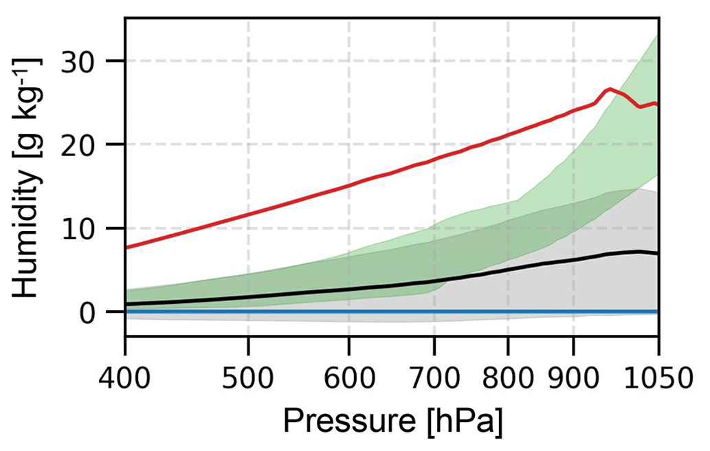
Figure 1 Statistical comparisons of the water vapor profiles from the ECMWF 83-profile dataset and the seven additional profiles from the UMBC 48-profile dataset. The red, black, and blue lines represent the maximum, mean, and minimum values of the ECMWF 83-profile dataset, respectively. The gray-shaded area indicates the range within twice the standard deviation of the ECMWF 83-profile dataset. The green-shaded area represents the range bounded by the maximum and minimum values of the seven additional profiles from the UMBC 48-profile dataset.

MonoRTM (Clough et al., 2005) is employed to calculate LBL transmittance at seven observed zenith angles (0, 36, 48, 55, 60, 63, 70°). Water vapor absorption, oxygen absorption, ozone line absorption, and nitrogen continuum absorption are considered. In MonoRTM, line absorption calculation relies on the HITRAN database (Gordon et al., 2022), and continuum absorption is handled by the MT_CKD continuum model (Mlawer et al., 2012; Clough et al., 2005). As channel-dependent spectral response functions (SRFs) are not available, the transmittance of GMRs' channels is calculated as the mean of the monochromatic transmittance across the channel bandwidth V:

$$\begin{array}{}\text{(4)}& {\mathrm{\Gamma }}_{\mathrm{ch},j}={\displaystyle \frac{{\int }_V{\mathrm{\Gamma }}_j\left(v\right)\mathrm{d}v}{{\int }_V\mathrm{d}v}},\end{array}$$

where the subscript j refers to the transmittance from the surface to the jth level. Γ_ch,j is the transmittance of an observed channel, and Γ_j(v) is the monochromatic transmittance. In practice, the channel bandwidth V is divided into 256 intervals, and the integral in Eq. (4) is approximated by a discrete sum.

In ARMS-gb, water vapor is the only variable gas, while other gases are fixed during the training process. As a result, the total transmittance can be written as

$$\begin{array}{}\text{(5)}& {\mathrm{\Gamma }}_{\mathrm{ch},j}^{\mathrm{total}}={\displaystyle \frac{{\mathrm{\Gamma }}_{\mathrm{ch},j}^{\mathrm{total}}}{{\mathrm{\Gamma }}_{\mathrm{ch},j}^{\mathrm{mixed}}}}{\mathrm{\Gamma }}_{\mathrm{ch},j}^{\mathrm{mixed}},\end{array}$$

where ${\mathrm{\Gamma }}_{\mathrm{ch},j}^{\mathrm{total}}$ and ${\mathrm{\Gamma }}_{\mathrm{ch},j}^{\mathrm{mixed}}$ are the total transmittance and the transmittance of all fixed gases, respectively. Following McMillin et al. (1995), we define the effective transmittance of water vapor ${\mathrm{\Gamma }}_{\mathrm{ch},j}^{{\mathrm{H}}_{\mathrm{2}}\mathrm{O},*}$ as

$$\begin{array}{}\text{(6)}& {\mathrm{\Gamma }}_{\mathrm{ch},j}^{{\mathrm{H}}_{\mathrm{2}}\mathrm{O},*}={\displaystyle \frac{{\mathrm{\Gamma }}_{\mathrm{ch},j}^{\mathrm{total}}}{{\mathrm{\Gamma }}_{\mathrm{ch},j}^{\mathrm{mixed}}}}.\end{array}$$

Both the water vapor absorption and the overlap absorption are included in ${\mathrm{\Gamma }}_{\mathrm{ch},j}^{{\mathrm{H}}_{\mathrm{2}}\mathrm{O},*}$. A linear regression is applied to fit layer optical depth related to ${\mathrm{\Gamma }}_{\mathrm{ch},j}^{\mathrm{mixed}}$ and ${\mathrm{\Gamma }}_{\mathrm{ch},j}^{{\mathrm{H}}_{\mathrm{2}}\mathrm{O},*}$ as follows:

$$\begin{array}{}\text{(7)}& d_j=D_j-D_{j+\mathrm{1}}=\sum _{i=\mathrm{1}}^{N_p}{C}_{i,j}{X}_{i,j},\end{array}$$

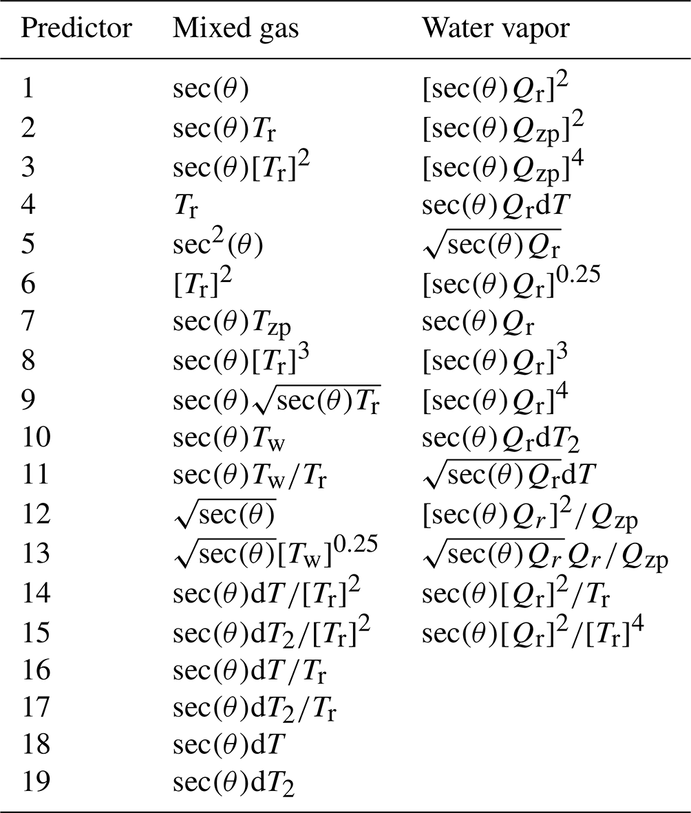
where d_j is the layer optical depth of the jth layer that is bounded by the jth level and the (j+1)th level. $D_j=-\ln \left({\mathrm{\Gamma }}_{\mathrm{ch},j}\right)$ is the optical depth from the surface to the jth level. X_i,j and C_i,j are predictors and corresponding fitting coefficients, respectively. To achieve high accuracy, we construct a predictor pool first and then use the backward stepwise regression to select the optimal combination of predictors. Detailed information about the predictor pool can be found in Appendix A. Both the transmittance calculation and the linear regression are performed at fixed 101 pressure levels. These pressure levels are identical to those used in RTTOV-gb (De Angelis et al., 2016), which are denser below 2 km.

Most NWP and reanalysis data have their own vertical coordinates, whereas optical depth calculations are constrained to the 101 levels. Consequently, in the ODPS simulation process, temperatures and water vapors from input pressure levels are remapped onto the 101 levels using the Rochon interpolation (Rochon et al., 2007) for the purpose of calculating predictors. After the optical depth calculations, the resulting D_j values are interpolated back to the original input pressure levels via a nearest-neighbor log-linear interpolation.

GMRs are sensitive to atmospheric parameters near the surface. To improve simulation accuracy, temperatures and water vapor values at a height of 2 m above ground level are used to correct the predictor values of the first layer above the surface. Furthermore, Kan et al. (2024) have shown that the logarithm of partial pressure is more effective than mass or volume mixing ratios in describing the vertical distribution of water vapor. In line with this finding, the unit of water vapor is converted to partial pressure, followed by a vertical interpolation of the logarithm of water vapor partial pressure to the 101 levels. The impact of this vertical interpolation on both the forward simulation and the Jacobian calculation is discussed in Sect. 3.

2.3 Jacobian calculation

Jacobian calculation is a crucial component of an RTM. It is essential for inversion and data assimilation. The aim of this calculation is to construct a K matrix that quantifies the sensitivity of radiances or BTs at each channel with respect to all input parameters. The K matrix can be represented as

$$\begin{array}{}\text{(8)}& \mathbf{K}=\left[\begin{array}{cccc}\partial I_{\mathrm{1}}/\partial x_{\mathrm{1}}& \partial I_{\mathrm{2}}/\partial x_{\mathrm{1}}& \mathrm{\dots }& \partial I_N/\partial x_{\mathrm{1}}\\ \partial I_{\mathrm{1}}/\partial x_{\mathrm{2}}& \partial I_{\mathrm{2}}/\partial x_{\mathrm{2}}& \mathrm{\dots }& \partial I_N/\partial x_{\mathrm{2}}\\ \mathrm{\dots }& \mathrm{\dots }& \mathrm{\dots }& \mathrm{\dots }\\ \partial I_{\mathrm{1}}/\partial x_M& \partial I_{\mathrm{2}}/\partial x_M& \mathrm{\dots }& \partial I_N/\partial x_M\end{array}\right],\end{array}$$

where N and M denote the number of channels and input parameters, respectively. For RT simulations, N is generally much less than M. In four-dimensional variational data assimilation systems, the K matrix is handled by the tangent linear module and the adjoint module (Errico, 1997). The tangent linear module computes how small changes in the input parameters affect the RTM output. It is developed by deriving the derivatives for each step in the RTM. For example, in RT simulations, an input parameter x_j contributes to the radiance vector I along the path

$$\begin{array}{}\text{(9)}& x_j\to \mathit{d}\to \mathit{I},\end{array}$$

where d and I represent the vector of optical depth and radiance at each channel. Correspondingly, the tangent linear module can be expressed as

$$\begin{array}{}\text{(10)}& x_{\mathrm{TL},j}\to {\displaystyle \frac{\partial \mathit{d}}{\partial x_j}}\cdot x_{\mathrm{TL},j}\to {\displaystyle \frac{\partial \mathit{I}}{\partial \mathit{d}}}\cdot {\displaystyle \frac{\partial \mathit{d}}{\partial x_j}}\cdot x_{\mathrm{TL},j}.\end{array}$$

The adjoint module is the backward counterpart of the tangent linear module. It computes how small changes in the RTM output affect the input parameters. This process is represented as

$$\begin{array}{}\text{(11)}& I_{\mathrm{AD},i}\to {\displaystyle \frac{\partial I_i}{\partial \mathit{d}}}\cdot I_{\mathrm{AD},i}\to {\displaystyle \frac{\partial I_i}{\partial \mathit{d}}}\cdot {\displaystyle \frac{\partial \mathit{d}}{\partial \mathit{x}}}\cdot I_{\mathrm{AD},i},\end{array}$$

where $\mathit{x}=\left[\begin{array}{cccc}{x}_{\mathrm{1}}& x_{\mathrm{2}}& \mathrm{\dots }& x_M\end{array}\right]$ is a vector containing all input parameters. In practice, the tangent linear module is developed first, and the adjoint module is subsequently derived from it.

The tangent linear and the adjoint modules work together to update the initial state of NWP based on observational data in four-dimensional variational data assimilation systems. The tangent linear module is used to evaluate how perturbations in the state evolve, while the adjoint model determines how these perturbations should be adjusted to minimize the difference between the RTM output and the actual observations.

3 Accuracy evaluation of ARMS-gb

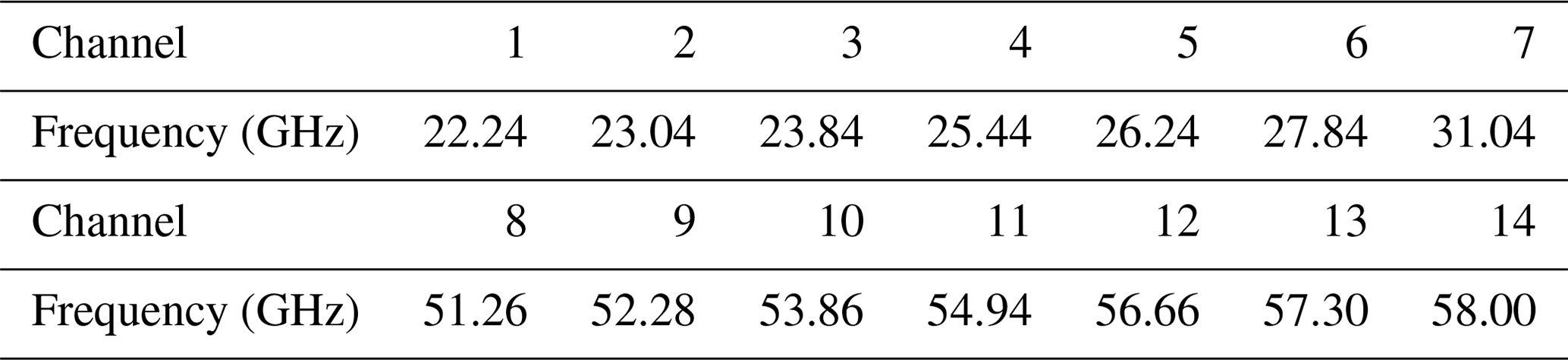
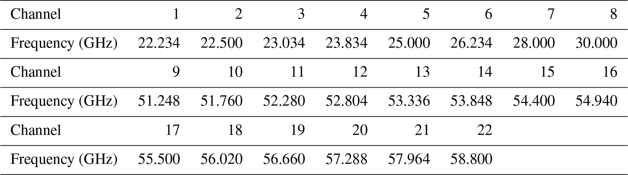
In this section, we evaluate the accuracy of ARMS-gb by comparing its results to those of MonoRTM and demonstrate the improvements achieved by enriching the training dataset. Additionally, we analyze the impact of vertical interpolation on both forward simulations and Jacobian calculations. These evaluations are performed using two datasets: the ECMWF 83-profile dataset and the UMBC 48-profile dataset. Our analysis includes results at seven observed zenith angles: 0, 36, 48, 55, 60, 63, and 70°. ARMS-gb currently supports two types of GMRs: the Humidity And Temperature PROfiler (HATPRO) and MP-3000A. The HATPRO, developed by Radiometer Physics GmbH, has seven K-band channels (channels 1–7) and seven V-band channels (channels 8–14). The center frequencies for each channel of the HATPRO are listed in Table 1. The MP-3000A, designed by Radiometrics, provides observations at 22 distinct channels. The center frequencies for each channel of the MP-3000A are presented in Table 2. Regarding bandwidths, the HATPRO has different values for its channels: 230 MHz for channels 1–11, 600 MHz for channel 12, 1000 MHz for channel 13, and 2000 MHz for channel 14. In contrast, all channels of the MP-3000A have a uniform bandwidth of 300 MHz.

Table 1 Center frequencies of HATPRO.

Table 2 Center frequencies of MP-3000A.

To evaluate the accuracy of ARMS-gb, we use three metrics: mean bias (AVG), standard deviation (SD), and root mean square error (RMSE). These metrics are calculated as follows:

$$\begin{array}{}\text{(12)}& {\displaystyle }\mathrm{AVG}& {\displaystyle }={\displaystyle \frac{{\sum }_{i=\mathrm{1}}^{N_{\mathrm{S}}}\left[{\mathrm{BT}}_{\mathrm{ben}}\right(i)-{\mathrm{BT}}_{\mathrm{sim}}(i\left)\right]}{N_{\mathrm{S}}}},\text{(13)}& {\displaystyle }\mathrm{SD}& {\displaystyle }=\sqrt{{\displaystyle \frac{{\sum }_{i=\mathrm{1}}^{N_{\mathrm{S}}}\left[{\mathrm{BT}}_{\mathrm{ben}}\right(i)-{\mathrm{BT}}_{\mathrm{sim}}(i)-\mathrm{AVG}{]}^{\mathrm{2}}}{N_{\mathrm{S}}}}},\text{(14)}& {\displaystyle }\mathrm{RMSE}& {\displaystyle }=\sqrt{{\displaystyle \frac{{\sum }_{i=\mathrm{1}}^{N_{\mathrm{S}}}\left[{\mathrm{BT}}_{\mathrm{ben}}\right(i)-{\mathrm{BT}}_{\mathrm{sim}}(i){]}^{\mathrm{2}}}{N_{\mathrm{S}}}}},\end{array}$$

where N_S is the total number of samples. BT_ben values are the benchmark values of BTs, and BT_sim values are simulated BTs. The benchmark values are calculated using MonoRTM through the following steps: (1) calculate the monochromatic radiance I(v); (2) integrate the monochromatic radiance over the channel bandwidth V to obtain the channel-averaged radiance

$$\begin{array}{}\text{(15)}& I_{\mathrm{ch}}={\displaystyle \frac{{\int }_{V}I\left(v\right)\mathrm{d}v}{{\int }_V\mathrm{d}v}},\end{array}$$

where I_ch is the channel-averaged radiance. Similar to Eq. (4), the integral calculation in Eq. (15) is also discretized as a sum, with the channel bandwidth V divided into 256 intervals prior to summation.

3.1 Effect of enriching the training dataset

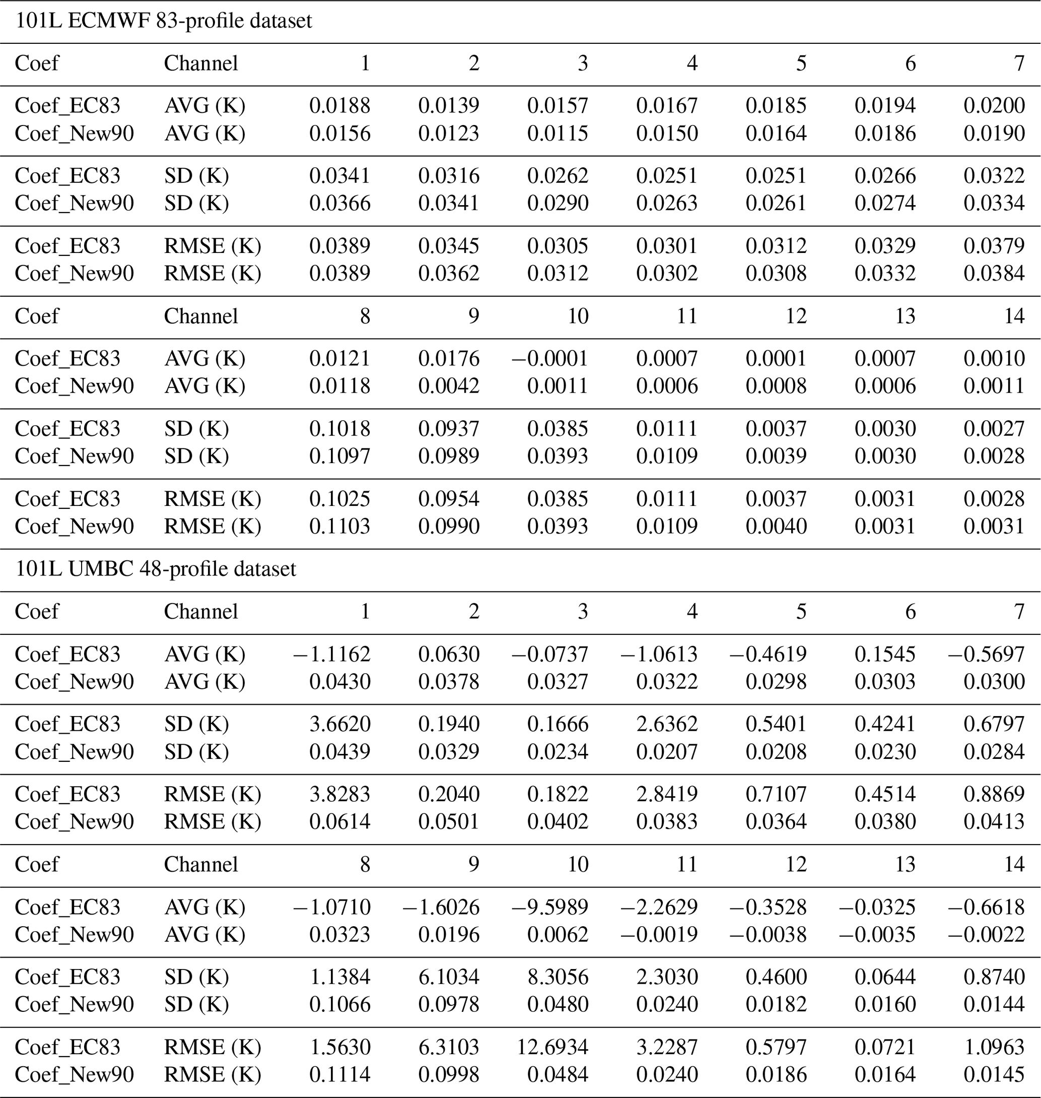
To evaluate the impact of enriching the training dataset, we trained two sets of fitting coefficients: one using the ECMWF 83-profile dataset (hereafter referred to as Coef_EC83) and the other using the new training dataset (hereafter referred to as Coef_New90). RT simulations based on these two coefficients are intercompared using the 101-level (101L) ECMWF 83-profile and UMBC 48-profile datasets. The 101 pressure levels are specifically chosen to eliminate effects related to vertical interpolation. The AVG, SD, and RMSE for each HATPRO channel are presented in Table 3. For the 101L ECMWF 83-profile dataset, the accuracy of the two fitting coefficients is comparable, with the maximum RMSE difference between them being only 0.0078 K. Both coefficients achieve high accuracy: in channels 1–7 and 10, the RMSE is approximately 0.03 K, while in channels 11–14, the RMSE is less than 0.012 K. However, biases are slightly larger in channels within the 51–54 GHz range, with the maximum RMSE exceeding 0.1 K in channel 9. This larger bias is attributed to the combined influence of temperature and water vapor, which reduces the correlation of layer opacity (De Angelis et al., 2016). For the 101L UMBC 48-profile dataset, results using Coef_New90 demonstrate significantly higher accuracy compared to those using Coef_EC83. In channels 9 and 10, the RMSE values for Coef_EC83 exceed 6.0 K, whereas those for Coef_New90 remain below 0.1 K. In other channels, the RMSE values for Coef_New90 are 1 to 2 orders of magnitude smaller than those for Coef_EC83. Large biases for Coef_EC83 in channel 10 may be caused by a strong interaction between water vapor and fixed gas transmittance. Since similar results are observed for MP-3000A channels, these results are not presented in the paper.

Table 3 AVG, SD, and RMSE of each channel of HATPRO. RT simulations based on Coef_EC83 and Coef_New90 are performed under the 101L ECMWF 83-profile and UMBC 48-profile datasets. MonoRTM serves as a benchmark for providing reference values for the comparison.

3.2 Effect of vertical interpolation

To apply ODPS in RT simulations with profiles having different kinds of vertical coordinates, two vertical interpolations are required. Previous studies have investigated the impact of different vertical interpolation modes on RT simulations and Jacobian calculations for the satellite perspective. For instance, Hocking (2014) compared five vertical interpolation modes within RTTOV. They found that using various vertical interpolation modes not only affects the simulated BTs, but also impacts Jacobian calculations. This study aims to compare BTs and Jacobians calculated by two different vertical interpolation modes for the GMR perspective. Detailed setups in these modes are summarized as follows.

Mode 1 is the default setting in RTTOV-gb (De Angelis et al., 2016; Cimini et al., 2019). The RTTOV-gb user guide also strongly recommends not to change the mode. In mode 1, both atmospheric parameters and optical depth are interpolated using the Rochon interpolation (Rochon et al., 2007).

Mode 2, which is employed by ARMS-gb, has previously been introduced (see Sect. 2.2). In mode 2, atmospheric parameters are interpolated using the Rochon interpolation, similar to mode 1. However, for optical depth, the nearest-neighbor log-linear interpolation is used instead. Additionally, before interpolating water vapor, its unit is converted to partial pressure, which allows for more accurate calculations.

We implement both interpolation modes within ARMS-gb first and perform comparisons across HATPRO channels. Atmospheric parameters are taken from the 54L ECMWF 83-profile and UMBC 48-profile datasets. For the benchmark calculations, we directly input 54L temperatures and water vapor profiles into MonoRTM without any interpolation. Both mode 1 and mode 2 interpolate profiles into 101L first and then interpolate optical depth back to 54L. To isolate the impact of the interpolation modes and exclude differences related to the training process (e.g., LBL RTMs and the training dataset), only Coef_New90 is used. Figure 2a and b illustrate results for the 54L ECMWF 83-profile dataset. In this case, mode 2 generally outperforms mode 1 in terms of accuracy. In K-band channels, both AVGs and SDs of mode 2 are significantly lower than those of mode 1. In channel 4, the AVG and SD of mode 2 are 0.19 and 0.15 K lower, respectively, compared to mode 1. In channels 8 and 9, the AVG for mode 1 is about 0.45 K, while mode 2 reduces this bias to less than 0.01 K. SDs in these channels also show slight reductions when mode 2 replaces mode 1. This modest reduction in SD is primarily attributed to the ODPS regression error, which can reach up to 0.1 K in these channels. Comparisons are also performed under the 54L UMBC 48-profile dataset, which includes profiles with high water vapor content. In channel 3, both the AVG and the SD for mode 1 are 0.27 K, whereas mode 2 achieves significantly lower values of 0.04 K and 0.03 K, respectively. In channel 8, the AVG for mode 1 reaches as high as 0.55 K, while mode 2 reduces this bias to just 0.03 K. Overall, the results indicate that mode 2 is generally more accurate than mode 1, particularly in channels with strong water vapor absorption.

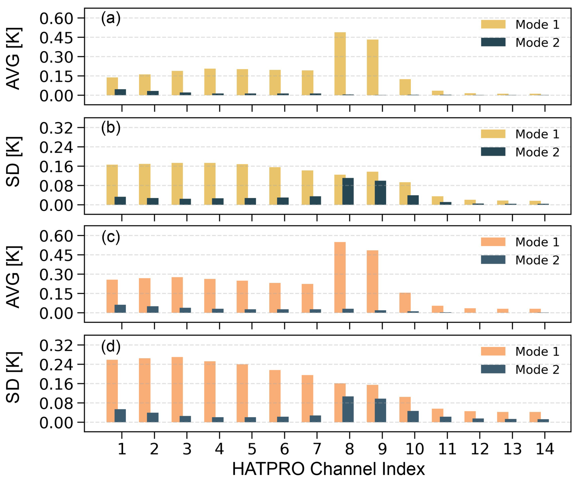
Figure 2 (a, b) AVGs and SDs of simulated BTs at seven observed zenith angles in HATPRO channels. RT simulations for interpolation modes 1 and 2 are performed under the 54L ECMWF 83-profile dataset. MonoRTM serves as a benchmark for providing reference values for comparison. (c, d) Same as (a) and (b) but with RT simulations performed under the 54L UMBC 48-profile dataset.

The Jacobians calculated by the two interpolation modes are also different. To evaluate this difference, we use the sixth profile in the 54L UMBC 48-profile dataset. The profile is selected because it produces significant BT differences between the two modes. The difference reaches up to 0.59 K at an observed zenith angle of 0° in channel 1. Figure 3a, b, and c show water vapor Jacobian at channels 3, 6, and 10, respectively. Jacobian differences between mode 1 and mode 2 are also shown. The results indicate that simulated BTs at channel 3 are very sensitive to water vapor located between 800 and 1000 hPa. The values of the water vapor Jacobian in this height range can exceed 5 K (log(g kg⁻¹))⁻¹. The maximum value of the water vapor Jacobian can reach 7.06 K (log(g kg⁻¹))⁻¹ in channel 3, while it is only 1.32 K (log(g kg⁻¹))⁻¹ in channel 10. The maximum value of the difference between the two modes occurs at the first level above the ground surface and reaches up to 0.61 K (log(g kg⁻¹))⁻¹ in channel 3, 0.55 K (log(g kg⁻¹))⁻¹ in channel 6, and 0.14 K (log(g kg⁻¹))⁻¹ in channel 10. Situations of temperature Jacobian in channel 11, channel 12, and channel 14 are shown in Fig. 3d, e, and f, respectively. The simulated BTs at these channels are sensitive to near-surface temperatures below 900 hPa. The maximum values of the temperature Jacobian occur at 1033 hPa and can reach up to 0.14 K K⁻¹ in channel 11, 0.24 K K⁻¹ in channel 12, and 0.28 K K⁻¹ in channel 14. Comparing mode 1 with mode 2, we find that mode 2 reduces the temperature Jacobian of channel 14 by 0.007 K K⁻¹ at 1013 hPa but gives an increase of 0.01 K K⁻¹ at 1050 hPa. Similar results are also found in channels 11 and 12 but with smaller amplitudes.

Due to its similarity to that for the HATPRO channels, analysis for the MP-3000A channels is not presented in the paper.

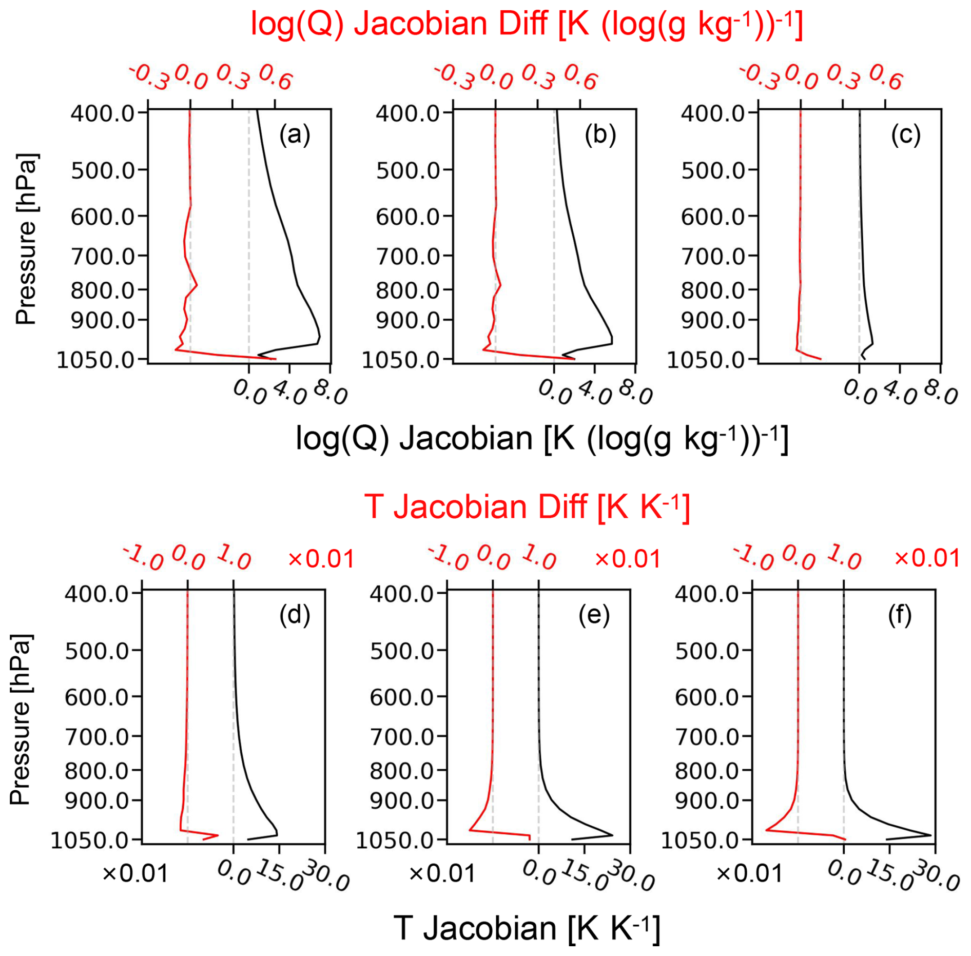
Figure 3 (a, b, c) Water vapor Jacobian analysis for channels 3, 6, and 10 of HATPRO. The water vapor Jacobian based on mode 2 is presented as black lines, and Jacobian differences between the two interpolation modes (mode 2 minus mode 1) are presented as red lines. (d, e, f) Same as (a), (b), and (c) but for temperature Jacobian analysis in different channels. The focus is on channel 11, channel 12, and channel 14 of HATPRO. RT simulations are performed under the sixth profile in the 54L UMBC 48-profile dataset. The observed zenith angle is set to 0°.

4 Applications in simulating real observations

In this section, we employ ARMS-gb to simulate real observations from GMRs in China. Three GMRs are selected: two are used to provide benchmark values for comparing the accuracy of ARMS-gb and RTTOV-gb, while the third is utilized to demonstrate the ability of ARMS-gb to monitor observational quality. The temperature and water vapor profiles, required as input for RT simulations, are derived from the 137L ERA5 reanalysis dataset. Additionally, direct observations of pressure, temperature, and humidity near the surface, provided by the meteorological sensor on board GMRs, are also utilized in the RT simulations in this study.

The ERA5 reanalysis dataset (Hersbach et al., 2020) provides an exceptionally detailed representation of the atmosphere, with its 137 vertical levels extending from the surface up to 0.01 hPa. These levels are not uniformly spaced and are more densely packed near the Earth's surface, allowing for a high vertical resolution that accurately captures atmospheric conditions in this height range. This configuration is particularly well-suited for simulating GMRs' observations, as it enables accurate modeling of the PBL. In this study, ERA5 is used with a temporal resolution of 1 h and a horizontal resolution of 0.25°×0.25°.

Prior to analyzing OMB based on RT simulations, two essential steps are performed: strict collocation and cloud detection. Collocation involves ensuring that the time and spatial matches between ERA5 reanalysis data and GMR observations are precise. To mitigate biases caused by temporal differences, only observations from GMRs on the hour are selected for analysis. A bilinear interpolation technique is applied to convert atmospheric profiles from the four nearest ERA5 grid points to the specific location of a GMR, using Euclidean-distance-based interpolation weights. Cloud detection involves rejecting observations that meet certain criteria: (1) observations during rain, which are flagged by rain sensors (Cimini et al., 2019); (2) observations with a high sky infrared temperature ($>-$30°C) (Martinet et al., 2015; De Angelis et al., 2016); and (3) observations with a standard deviation of BTs in the window channel (near 31 GHz) exceeding 0.2 K over a 10 min period (Turner et al., 2007; Cimini et al., 2019). In addition, total column cloud liquid water content and ice water content from the ERA5 reanalysis dataset are used as another index for cloud clearing. The threshold is set to 100 g m⁻² according to Moradi et al. (2020). We also evaluated OMB statistics under different thresholds (e.g., 10 g m⁻², 1 g m⁻²) and results do not noticeably change.

4.1 Comparison to RTTOV-gb

RTTOV-gb is a fast RTM developed at the Center of Excellence in Telesensing of Environment and Model Prediction of Severe Events (CETEMPS). It accounts for gaseous absorption by ODPS, which is trained by R98 (Rosenkranz, 1998) or R17 (Rosenkranz, 2017). Additionally, the effects of clouds on observed microwave BTs are also included in RTTOV-gb. A detailed description of the model can be found in De Angelis et al. (2016) and Cimini et al. (2019). For a comprehensive comparison between ARMS-gb and RTTOV-gb, refer to Table 4, which summarizes their similarities and differences. In this study, coefficients trained by R98 is used for running RTTOV-gb. It is worth comparing the results of ARMS-gb with those of RTTOV-gb using coefficients trained by R17, a comparison we plan to conduct soon.

The intercomparison period spans 1 November 2023 to 30 April 2024, covering both winter and spring seasons. Two GMR stations are selected for this study: Karamay, Xinjiang (45.61° N, 84.85° E) and Tanggu, Tianjin (35.16° N, 117.79° E). The altitudes above sea level are 451.6 m for Karamay and 27 m for Tanggu. The SD of surface pressures from the four nearest ERA5 grid points is approximately 15 hPa for Karamay and 5 hPa for Tanggu, which reflects the situation of surrounding orography. The climate at these two locations is distinct. Karamay has a dry continental climate with low humidity. In contrast, Tanggu experiences a temperate semi-humid monsoon climate with higher humidity. These two stations serve as representative examples of dry and relatively moist environments. The GMRs at both stations provide vertical measurements with an observed zenith angle of 0°. The selection of both time period and station makes it suitable for comparing the performance of ARMS-gb and RTTOV-gb in different atmospheric conditions. Due to the stability of the OMB trend during this period, it is assumed that the quality of the calibration may be stable.

The GMR at Karamay is Airda-HTG4. It operates with center frequencies and bandwidths identical to those of HATPRO. Following the collocation and cloud detection steps, a total of 1922 samples remain for analysis. Figure 4a–c present the OMB results obtained from both RTTOV-gb and ARMS-gb. Additionally, we calculate the daily SD using OMB over each individual day. The mean relative differences in daily SD between RTTOV-gb and ARMS-gb are depicted in Fig. 4d–f. To assess the statistical significance of these differences, Student's t test is performed, and the corresponding 95 % confidence interval is indicated. This allows for a more rigorous evaluation between the two RTMs.

Table 4 The similarities and differences between ARMS-gb and RTTOV-gb.

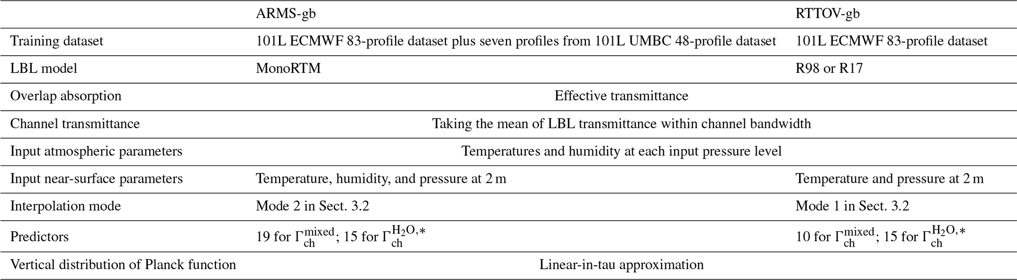
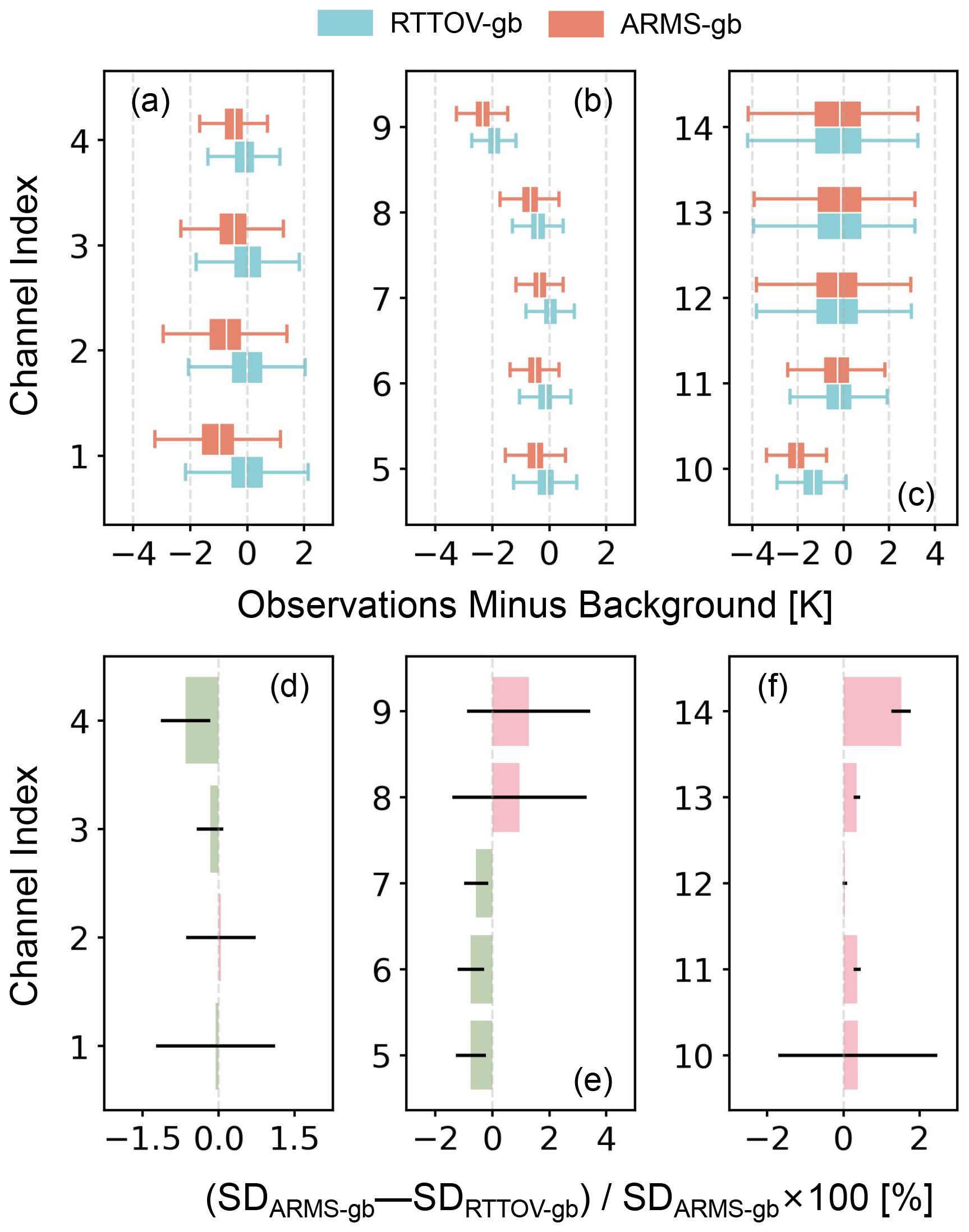
Figure 4 (a–c) OMB of RTTOV-gb and ARMS-gb during the period from 1 November 2023 to 30 April 2024. Observations are from Airda-HTG4 at Karamay. RT simulations are performed under the 137L ERA5 reanalysis dataset. White markers indicate the median values of each distribution. (d–f) Mean relative differences in daily SD between RTTOV-gb and ARMS-gb. Daily SD values are calculated using OMB within each single day. The black bars represent the 95 % confidence range, indicating the statistical significance of these differences.

The results shown in Fig. 4 highlight significant differences in the behavior of ARMS-gb and RTTOV-gb across various channels of Airda-HTG4 at Karamay. In channels 1–8, ARMS-gb tends to overestimate BTs. In contrast, the OMB median values of RTTOV-gb are much closer to 0 K in these channels. For instance, in channel 1, the OMB median value of ARMS-gb is −0.98 K, while for RTTOV-gb it is only −0.05 K. In channels 9 and 10, the absolute AVG values for ARMS-gb exceed 2 K. RTTOV-gb also overestimates BTs in these two channels, with AVGs of −1.93 K in channel 9 and −1.34 K in channel 10. Both ARMS-gb and RTTOV-gb demonstrate high accuracy in channels 11–14, where the OMB median values for both RTMs are less than 0.3 K. In terms of daily SD, significant differences between the two RTMs are observed in four K-band channels (channels 4–7) and three V-band channels (channels 11, 13, 14). Specifically, compared to RTTOV-gb, the daily SD of ARMS-gb is reduced by 0.75 % in channels 5 and 6. However, RTTOV-gb shows more stable OMBs than ARMS-gb in three V-band channels, with a mean relative difference in daily SD of 1.52 % in channel 14.

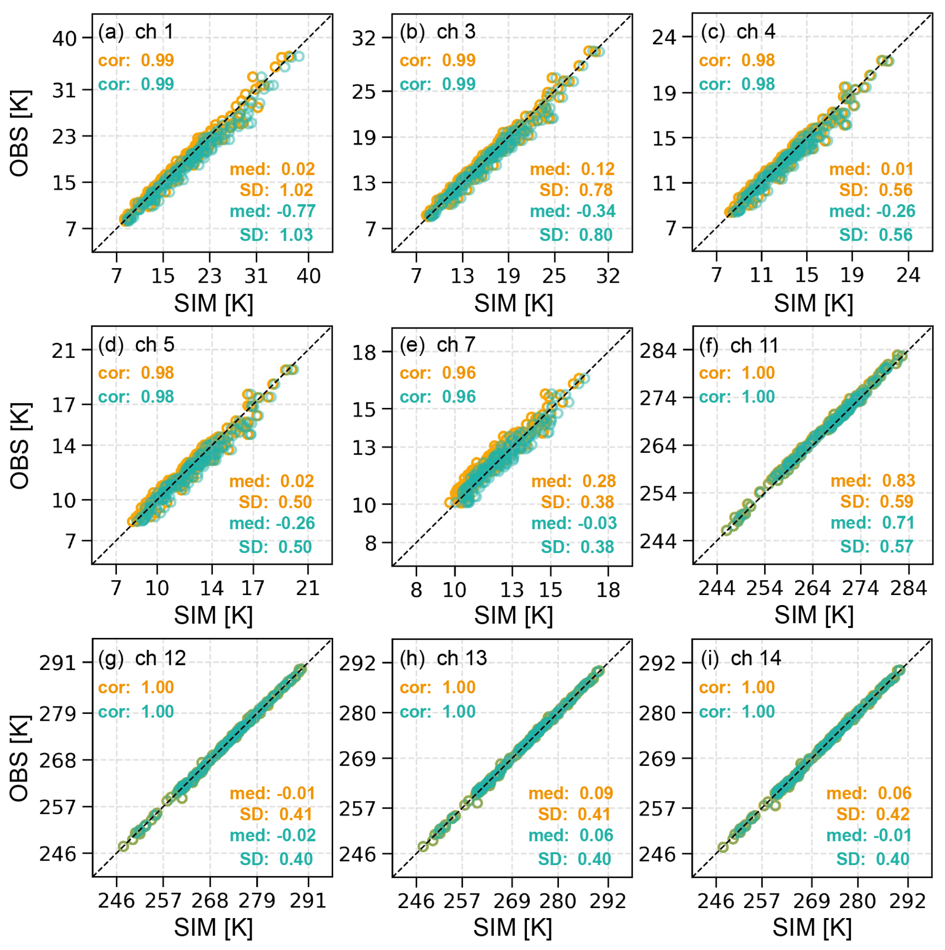
Figure 5 Scatter of simulated vs. observed BTs for 9 out of the 14 channels of Airda-HTG4 at Karamay from 1 November 2023 to 30 April 2024. RT simulations are performed using radiosonde data. Orange represents results of RTTOV-gb; green represents results of ARMS-gb. After collocation and cloud detection, a total of 163 samples are analyzed in this case. The panel reports the correlation coefficients (cor), as well as the median (med) values and standard deviations (SDs) of OMB.

Additionally, radiosonde data are also used as input for RT simulations, and the results from RTTOV-gb and ARMS-gb are compared. Scatterplots of simulated versus observed BTs are presented in Fig. 5, focusing on five K-band channels and four V-band channels. After collocation and cloud detection, 163 samples are evaluated. In the K-band channels, RTTOV-gb simulations align more closely with observations compared to ARMS-gb, exhibiting smaller OMB median values and SDs. ARMS-gb tends to overestimate observations, consistent with the results in Fig. 4. In the V-band channels, RT simulation accuracy is generally higher than in the K-band channels, with correlation coefficients approaching 1.0. The OMB median values and SDs from ARMS-gb are slightly lower than those from RTTOV-gb.

Figure 6 Same as Fig. 4 but showing the situation of YKW3 at Tanggu.

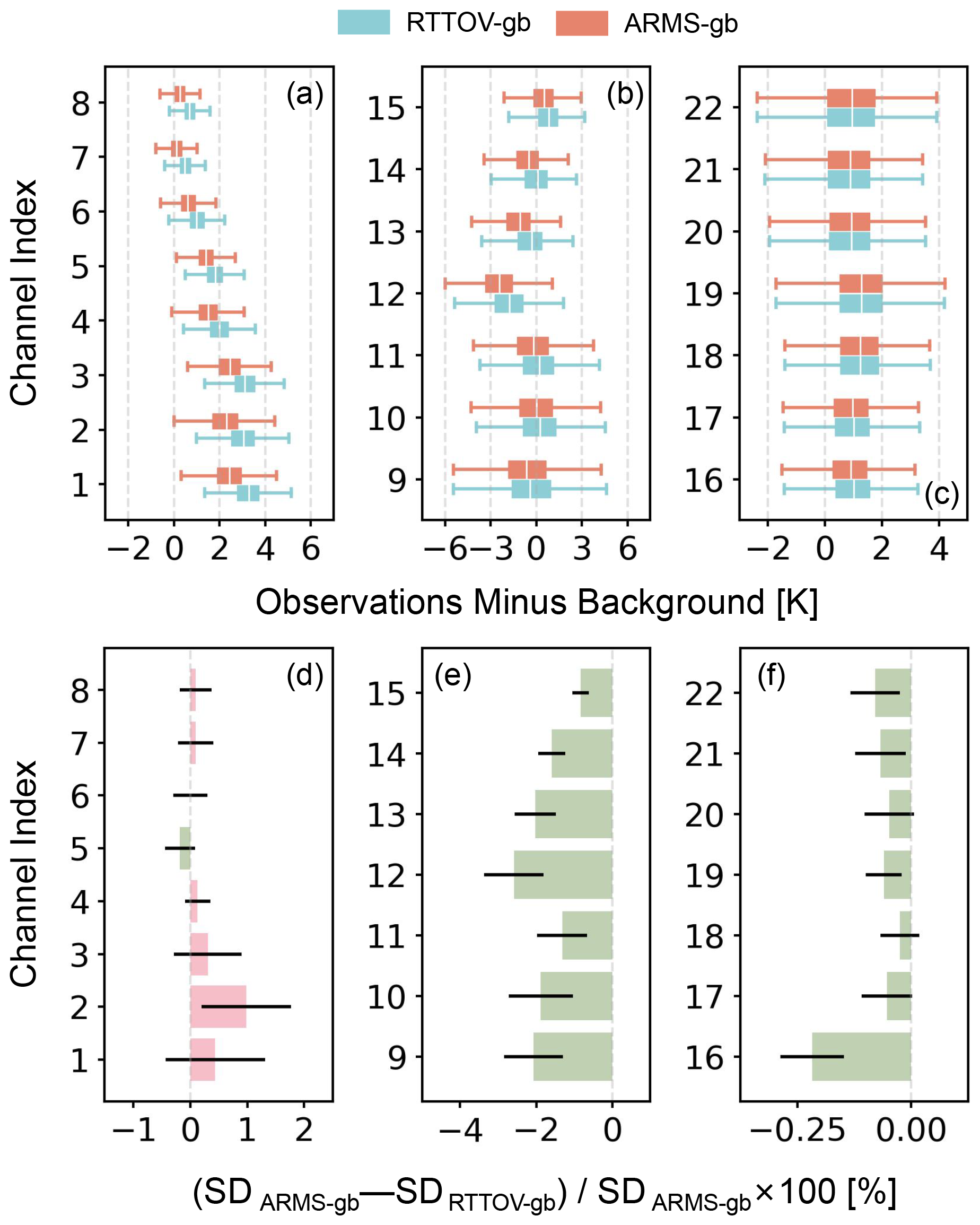
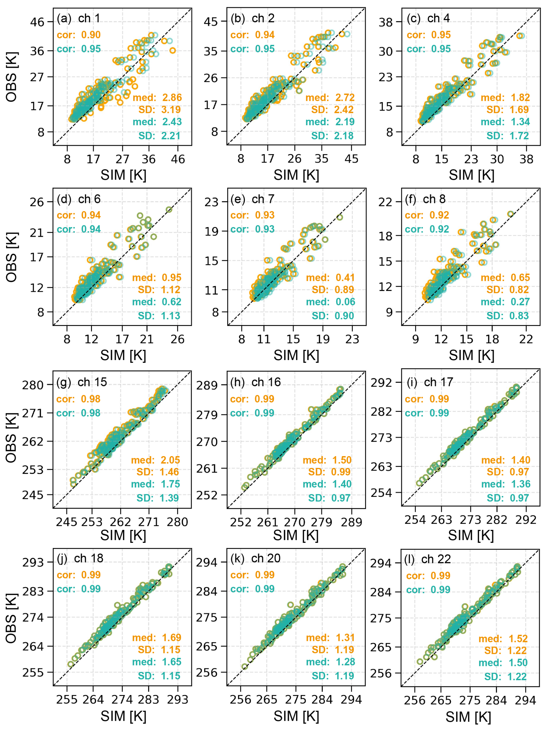
Figure 7 Same as Fig. 5 but showing results for 12 out of the 22 channels of YKW3 at Tanggu from 1 November 2023 to 30 April 2024. After collocation and cloud detection, a total of 148 samples are analyzed in this case.

The GMR at Tanggu, YKW3, shares the same center frequencies and bandwidths as MP-3000A. Figure 6a–c present the OMB results of the two RTMs based on 1845 statistical data. Notably, BTs simulated by ARMS-gb are more closely aligned with observations than those of RTTOV-gb in channels 1–8. In particular, the OMB median values of RTTOV-gb show significant deviations from 0 K, with values reaching 3.28 K in channel 1 and 0.69 K in channel 8. In contrast, ARMS-gb exhibits more accurate results, with OMB median values of 2.44 K in channel 1 and 0.26 K in channel 8. In channels 12, 13, and 14, the AVGs of RTTOV-gb are more closely aligned with 0 K than those of ARMS-gb. Both ARMS-gb and RTTOV-gb demonstrate similar accuracy in channels 16–22, with differences in OMB median values between the two RTMs being less than 0.1 K. Figure 6d–f show the mean relative differences in daily SD between ARMS-gb and RTTOV-gb. In channel 2, the daily SD of RTTOV-gb is 0.98 % lower than that of ARMS-gb. Conversely, in channels 9–16, the daily SD of ARMS-gb is significantly lower than that of RTTOV-gb, with the largest relative difference occurring in channel 12 at 2.59 %. The smallest relative difference occurs in channel 16, at 0.22 %. OMB results from ARMS-gb also show slightly greater stability than those of RTTOV-gb in channels 17–22.

Similar to the Karamay case, RT simulations for the Tanggu case are also conducted using radiosonde data. Simulated BTs from both ARMS-gb and RTTOV-gb are compared with observations, as shown in Fig. 7. After collocation and cloud detection, 148 samples are included in the comparison, with 12 out of the 22 channels selected for analysis. In channels 1 and 2, both RTTOV-gb and ARMS-gb underestimate BTs. However, ARMS-gb provides more accurate results than RTTOV-gb, with higher correlation coefficients and smaller OMB median values and SDs. In channels 4, 6, 7, and 8, the OMB median values from ARMS-gb are closer to 0 K, while RTTOV-gb shows smaller SDs of OMB. For channels with central frequencies ranging from 54.5 to 58.8 GHz, both RTTOV-gb and ARMS-gb accurately simulate observed BTs, with correlation coefficients for both RTMs reaching up to 0.98. The OMB median values and SD from ARMS-gb are slightly lower than those from RTTOV-gb. We would like to highlight that the calibration quality of YKW3 at Tanggu is not as sufficient as that of Airda-HTG4 at Karamay. Significant biases and considerable scatter are observed between YKW3 measurements and RT simulations based on radiosonde data. Improving the calibration quality remains a key challenge for the quantitative application of GMR observations.

The performance of fast RTMs is influenced by several factors. A detailed description of channel characteristics and accuracy of the LBL model used for training are crucial in achieving accurate RT simulations. Moreover, the quality of the input profiles themselves can be a significant limitation. For instance, temperatures from ERA5 reanalysis data have been shown to have large systematic errors at altitudes between 2000–3000 m and relative humidity errors ranging from 40 % to 100 % over the range of 500–2500 m (Wei et al., 2024). This highlights the challenge in relying on current reanalysis data for accurate thermal variables, particularly in the PBL. Furthermore, channel characteristics play a significant role in RT simulations, especially when considering the SRF information. Studies have demonstrated that incorporating SRF information can lead to substantial improvements in RT simulations from a satellite perspective (Moradi et al., 2020; Chen et al., 2021; Kan et al., 2024). We believe that incorporating SRF information could also enhance the accuracy of both RTTOV-gb and ARMS-gb.

4.2 Monitoring observational qualities

ARMS-gb offers real-time OMB information, which provides valuable guidance for evaluating observational qualities. This is particularly important in assimilating GMR data in NWP. In this study, ARMS-gb is applied to monitor the quality of observations from Airda-HTG4 located at Minfeng, Xinjiang (37.07° N, 82.69° E). The station's altitude above sea level is 1410 m, and the SD of surface pressures from the four nearest ERA5 grid points is about 6 hPa. The time period examined spans 1 September to 30 November 2023. After collocation and cloud detection, 1922 samples are retained for analysis.

The observational BTs and the OMB of ARMS-gb in channels 1, 8, and 14 are presented in Fig. 8. Channels 1 and 14 serve as representatives of water vapor and temperature channels, respectively, while channel 8 is influenced by both water vapor and temperature. Insights from the OMB results for channel 1 indicate that SD can be significantly reduced through calibration, decreasing from 2.03 to 0.98 K. The calibration time can also be clearly identified in the OMB series of channel 8. Both AVG and SD values change noticeably before and after the calibration time. Specifically, AVG and SD reach 4.60 and 0.61 K in September, respectively, but are reduced to −0.52 and 0.33 K after calibration. In contrast, observational BTs of channel 14 show little sensitivity to calibration. Both AVG and SD values for this channel remain largely unchanged, with only some negative OMB values occurring during a short time period around the calibration time. The observation series of these three channels highlights that it is challenging to evaluate the quality of observations without access to OMB information. The results from ARMS-gb provide valuable insights into observational qualities.

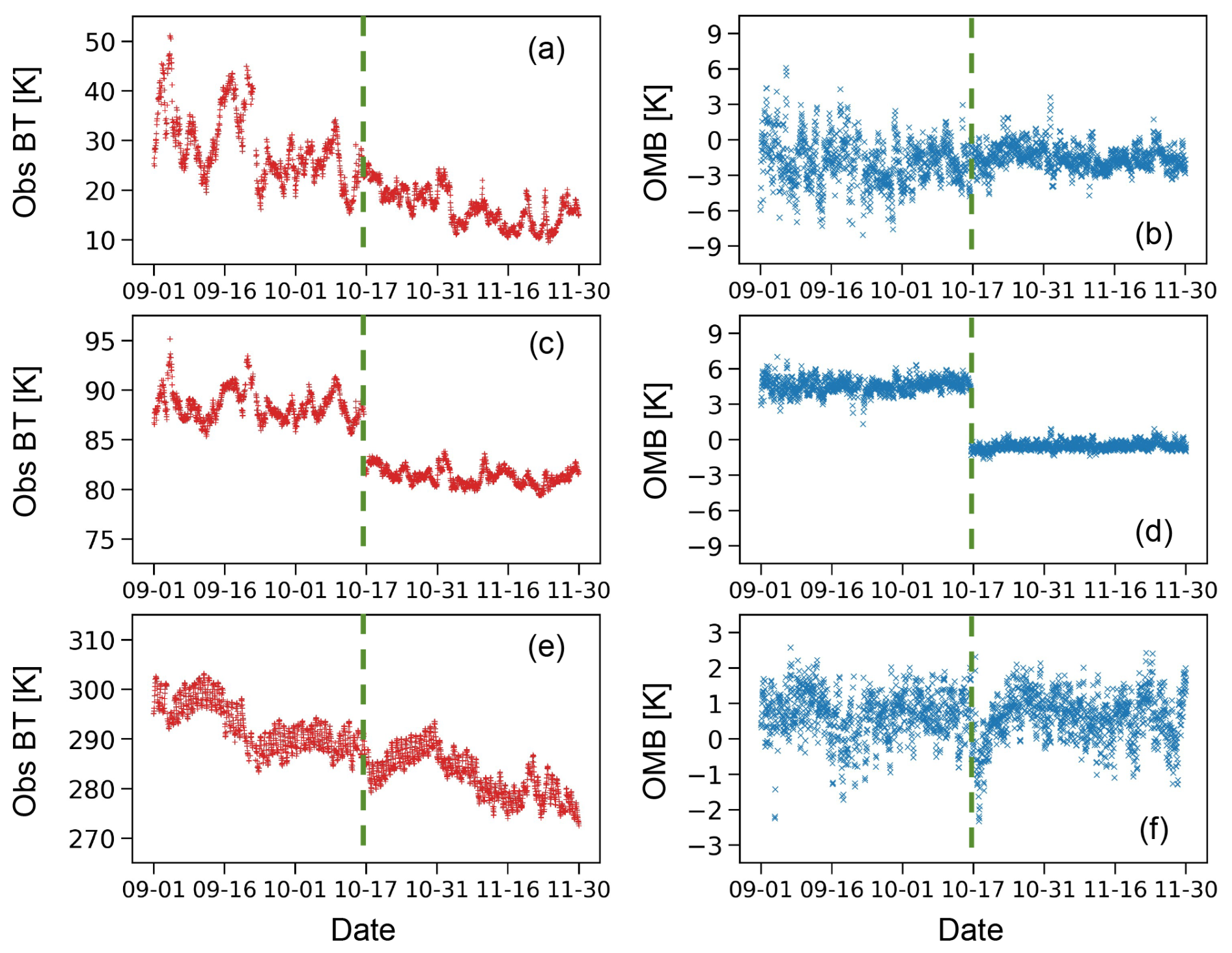
Figure 8 (a, b) Observations for channel 1 from Airda-HTG4 at Minfeng during 1 September to 30 November 2023 along with the corresponding OMB series of ARMS-gb. (c, d) Same as (a) and (b) but showing situations of channel 8. (e, f) Same as (a) and (b) but showing situations of channel 14. The dashed green line indicates the calibration time.

5 Summary and conclusions

GMRs can provide continuous observations with high temporal resolution. These observations are particularly useful for monitoring rapid changes in temperature and humidity within the PBL. As a result, direct assimilation of GMR observations has great potential in improving the performance of NWP, especially for the lowest few kilometers of the atmosphere. In this study, we propose an RTM, ARMS-gb, capable of simulating BTs observed by GMRs. ARMS-gb can be used as an observation operator to map atmospheric parameters onto observations in a data assimilation system.

ARMS-gb is developed based on a clear-sky RT solver that accounts for atmospheric thermal emissions from TOA to the ground surface, as well as the effects of gaseous absorption. An accurate description of gaseous absorption is critical for the performance of RT simulations. To address this issue, ARMS-gb employs ODPS, which utilizes the 101L ECMWF 83-profile dataset as its primary training dataset. This dataset is augmented with seven additional profiles from the 101L UMBC 48-profile dataset. The humidity range of these additional profiles exceeds the mean values plus the standard deviation of the ECMWF 83-profile dataset, particularly in the low levels of the troposphere. This augmentation enhances the simulation accuracy of ARMS-gb, particularly in moist environments. In ODPS, MonoRTM is employed to calculate the LBL transmittance at seven observed zenith angles. To apply ODPS in RT simulations with profiles having different types of vertical coordinates, two vertical interpolations are required. In ARMS-gb, temperatures and water vapors from input pressure levels are remapped onto the 101L using the Rochon interpolation for calculating predictors. The resulting optical depth values are interpolated back to the original input pressure levels via a nearest-neighbor log-linear interpolation. Additionally, before interpolating water vapor, its unit is converted to partial pressure, which allows for more accurate calculations. To satisfy the requirements of its applications in remote sensing and data assimilation, we also develop the tangent linear and adjoint module of ARMS-gb and derive the analytical K matrix.

ARMS-gb currently supports two types of GMRs: HATPRO and MP-3000A. To evaluate the impact of enriching the training dataset, two sets of fitting coefficients are trained: one using the ECMWF 83-profile dataset (Coef_EC83) and the other using the new training dataset (Coef_New90). Profiles from the 101L ECMWF 83-profile and UMBC 48-profile datasets are used as input for RT simulations. MonoRTM serves as the benchmark for providing reference values for comparison. For the 101L ECMWF 83-profile dataset, the accuracy of the two fitting coefficients is comparable, with the maximum RMSE difference between them being only 0.0078 K. However, for the 101L UMBC 48-profile dataset, Coef_New90 demonstrates significantly higher accuracy compared to Coef_EC83. The RMSE values of Coef_New90 are 1 to 2 orders of magnitude smaller than those of Coef_EC83. Additionally, the effects of vertical interpolation modes on forward and Jacobian calculations are evaluated from the perspective of HATPRO channels. Two different vertical interpolation modes are considered: mode 1, the default setting in RTTOV-gb, and mode 2, employed by ARMS-gb. To isolate the impact of the interpolation modes, only Coef_New90 is used to exclude differences related to the training process. Under the 54L ECMWF 83-profile dataset, mode 2 generally outperforms mode 1, particularly in channels with strong water vapor absorption. For example, in channel 4, the AVG and SD using mode 2 are 0.19 and 0.15 K lower, respectively, compared to mode 1. In channels 8 and 9, the AVG for mode 1 is approximately 0.45 K, while for mode 2 it is less than 0.01 K. SDs in these channels also show slight reductions when mode 1 is replaced with mode 2. The Jacobian values calculated by the two interpolation modes are also different. Comparing mode 1 with mode 2, it is observed that mode 2 reduces the temperature Jacobian of channel 14 by 0.007 K K⁻¹ at 1013 hPa but increases it by 0.01 K K⁻¹ at 1050 hPa. In terms of the water vapor Jacobian, the maximum difference between the two modes occurs at the first level above the ground surface. In channel 3, this difference reaches up to 0.61 K (log(g kg⁻¹))⁻¹, while in channel 10, it is only 0.14 K (log(g kg⁻¹))⁻¹.

To further validate the performance of ARMS-gb, we apply it in simulating real observations from GMRs and compare its results to those of RTTOV-gb. Input atmospheric parameters, such as temperature and water vapor profiles, are derived from the 137L ERA5 reanalysis dataset. The intercomparison period spans 1 November 2023 to 30 April 2024. Airda-HTG4, located at Karamay, Xinjiang (45.61° N, 84.85° E), and YKW3, located at Tanggu, Tianjin (35.16° N, 117.79° E), provide actual observations. Significant differences are observed in the behavior of ARMS-gb and RTTOV-gb across various channels of Airda-HTG4 at Karamay. In channels 1–8, ARMS-gb tends to overestimate BTs, whereas the OMB median values of RTTOV-gb are much closer to 0 K in these channels. Both RTMs demonstrate high accuracy in channels 11–14. In terms of daily SD, ARMS-gb outperforms RTTOV-gb in channels 5 and 6, reducing the daily SD by 0.75 %. However, in channel 14, the daily SD for ARMS-gb increased by 1.52 % compared to RTTOV-gb. Furthermore, radiosonde data are also used as input for RT simulations, and the results from RTTOV-gb and ARMS-gb are compared. In the K-band channels, ARMS-gb tends to overestimate observations, consistent with the results derived from the 137L ERA5 reanalysis dataset. RTTOV-gb simulations exhibit smaller OMB median values and SDs. In the V-band channels, simulations of both RTTOV-gb and ARMS-gb show high accuracy, with correlation coefficients approaching 1.0.

Under the 137L ERA5 reanalysis dataset, BTs simulated by ARMS-gb are more closely aligned with observations from YKW3 at Tanggu than those of RTTOV-gb in channels 1–8. The daily SD of ARMS-gb is lower than that of RTTOV-gb in channels 9–22, with the maximum relative difference observed in channel 12, reaching 2.59 %. Similar to the Karamay case, RT simulations are also conducted using radiosonde data for the Tanggu case. The results show that the OMB median values from ARMS-gb are closer to 0 K in most YKW3 channels. Notably, in channels 1 and 2, ARMS-gb provides more accurate results than RTTOV-gb, with higher correlation coefficients and smaller OMB median values and SDs. For channels with central frequencies ranging from 54.5 GHz to 58.8 GHz, both RTTOV-gb and ARMS-gb accurately simulate observed BTs, with correlation coefficients for both RTMs reaching up to 0.98.

To demonstrate the ability of ARMS-gb to monitor observational quality, we utilize observations from Airda-HTG4 located at Minfeng, Xinjiang (37.07° N, 82.69° E). The calibration time can be clearly identified in the OMB series of channels 1 and 8. In contrast, observational BTs of channel 14 show little sensitivity to calibration. Compared to observation series, OMB information from ARMS-gb provides more valuable insights into observational qualities of GMRs.

We believe that the performance of ARMS-gb can be further enhanced by incorporating SRF information into ODPS. Selecting a reliable and accurate LBL model for training is also essential for improving the accuracy of RT simulations. For example, Larosa et al. (2024) incorporate the latest advancements in absorption spectroscopy to improve RT simulation accuracy in the 50–54 GHz frequency range. An intercomparison among different microwave LBL RTMs is necessary to construct a reliable transmittance dataset for the ODPS training process. In addition, we plan to integrate a particle scattering module into ARMS-gb in the near future, which will extend its capabilities to enable simulations under all-sky conditions. With the development of ARMS-gb, research on the direct assimilation of GMR observations into NWP will be carried out soon.

Appendix A: Predictors for optical depth regression

In this section, predictors for optical depth regression are specified. These predictors also refer to Matricardi et al. (2004) and De Angelis et al. (2016).

In Table A1, θ is the local zenith angle. In the optical depth calculation, θ varies with height, and the Earth curvature effect is then taken into account (Chen et al., 2012).

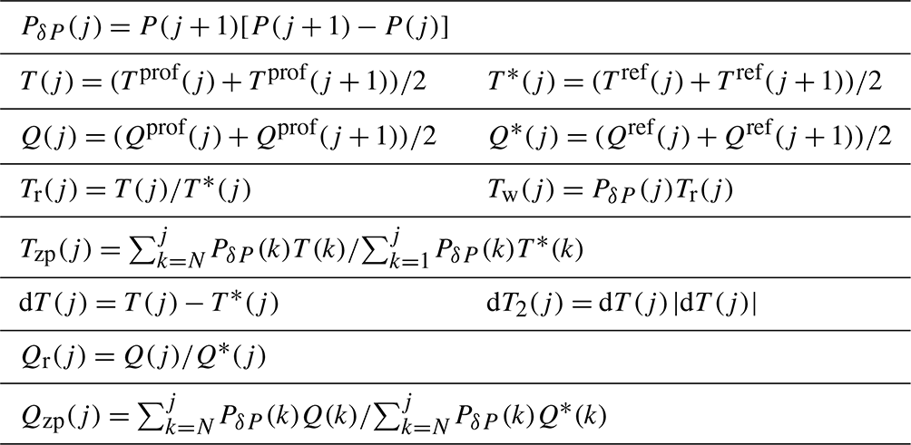
As mentioned in Sect. 2, the predictor calculation is performed on the fixed 101 levels. Correspondingly, in Table A2, j varies from 1 to 100 and refers to the jth atmospheric layer. T^prof (unit: K) and Q^prof (unit: g kg⁻¹) are the input temperature and water vapor mass mixing ratio. Both of them have been interpolated into the fixed 101 levels before the predictor calculation. T^ref and Q^ref are the same as T^prof and Q^prof but from the reference profile. The reference profile is usually obtained by taking the mean over the training dataset. We note that T_w(100) is set to 0 (De Angelis et al., 2016).

Table A1 The predictor pool used for optical depth regression.

Table A2 Variables used in the predictor calculation.