Simulation performance of planetary boundary layer schemes in WRF v4.3.1 for near-surface wind over the western Sichuan Basin: a single-site assessment

The topography of the Sichuan Basin is complex, and high-resolution wind field simulations over this region are of great significance for meteorology, air quality, and wind energy utilization. In this study, the Weather Research and Forecasting (WRF) model was used to investigate the performance of different planetary boundary layer (PBL) parameterization schemes in simulating near-surface wind fields over the Sichuan Basin at a spatial resolution of 0.33 km. The experiment is based on multiple case studies of a selection of 28 near-surface wind events from 2021 to 2022, and a total of 112 sensitivity simulations were carried out and compared to observations by employing four commonly used PBL schemes: the Yonsei University (YSU) scheme, the Mellor–Yamada–Janjić (MYJ) scheme, the Mellor–Yamada–Nakanishi–Niino level 2 (MYNN2) scheme, and the quasi-normal scale elimination (QNSE) scheme. The results demonstrate that the wind direction can be reasonably reproduced, and its sensitivity to the PBL scheme appears to be less pronounced compared to the near-surface wind speed, though some variability is still observed. As for wind speed, the QNSE scheme had the best performance in reproducing the temporal variation out of the four schemes, while the MYJ scheme had the smallest model bias. Further cluster analysis demonstrates that the sensitivity of the PBL schemes is affected by diurnal variation and different circulation geneses. For instance, when the near-surface wind event, caused by the southward movement of strong cold air, occurred between 06:00 and 08:00 UTC, the variation and speed were well reproduced by all four PBL schemes, and the differences between them were small. However, the simulation results for strong winds occurring during midnight to the early hours of the morning exhibit poor root mean square errors but high correlation coefficients, whereas for strong wind processes happening in the early to late evening hours and for southwesterly wind processes, the opposite pattern occurs. Overall, the four schemes are better for near-surface wind simulations in daytime than at night. The results show the role of PBL schemes in wind field simulations under unstable weather conditions and provide a valuable reference for further research in the study area and surrounding areas.

1 Introduction

Wind, as one of the fundamental natural phenomena in the atmosphere, not only poses hazards to civil aviation safety and maritime transportation during severe wind events (Manasseh and Middleton, 1999; Leung et al., 2020), but also impacts the dispersion of atmospheric pollutants directly near the surface, leading to adverse effects on public health and the environment (Liu et al., 2020; Coccia, 2020; Yang and Shao, 2021). Moreover, wind energy has attracted increasing attention because of its non-polluting and renewable nature, but due to the random nature of wind speed, wind power generation is intermittent, which poses security and stability challenges for large-scale integration of wind energy into the power network (Liu et al., 2019; Kibona, 2020; Shi et al., 2021). Therefore, accurate prediction of near-surface winds has become key to ensuring traffic safety, optimizing wind energy utilization, and evaluating air quality, and it is also an important scientific issue for disaster prevention and mitigation, economic benefits, and human life and health.

Near-surface wind fields are influenced by a combination of various factors (Zhang et al., 2021), including atmospheric dynamic and thermodynamic processes (such as pressure gradient force, temperature gradients, and so on), topography (such as geographical features, elevation), and underlying surface (such as vegetation, land use). As a state-of-the-art mesoscale weather prediction model, the Weather Research and Forecasting (WRF) model can predict the fine-scale structure of near-surface wind fields by simulating the evolution of various physical processes in the atmosphere, which is significantly better than the statistical prediction model that lacks a description of thermodynamic processes. Furthermore, there is a wealth of research on the prediction and simulation of the refined characteristics of local wind fields using the WRF model (Prieto-Herráez et al., 2020; Salfate et al., 2020; Xu et al., 2020; Tiesi et al., 2021; Wu et al., 2022; Yan et al., 2022; Mi et al., 2023). Although the simulation of near-surface wind fields involves the nonlinear interactions of various physical processes, the physical processes in the planetary boundary layer (PBL) play a direct role in influencing near-surface wind fields. As the interaction area between the atmosphere and the ground, the thermal and dynamic structure and the turbulent motion and mixing process in the boundary layer will directly affect the distribution of the near-surface wind field; therefore, the simulation of the boundary layer by the model can directly affect the accuracy of the near-surface wind field (Chen et al., 2020).

In the mesoscale model, since the employed grid scales and time steps cannot explicitly represent the spatiotemporal scales which turbulent eddies operate on, the PBL parameterization scheme was used to express the effects of turbulent eddies (Dudhia, 2014). The latest version (4.3.1) of the WRF model provides more than 10 kinds of PBL parameterization schemes, and the differences among them are mainly due to the different methods of dealing with the turbulence closure problem. In China, Ma et al. (2014) conducted a series of sensitivity simulations on spring strong wind events in Xinjiang Province using the Yonsei University (YSU), Mellor–Yamada–Janjić (MYJ), and Asymmetrical Convective Model, version 2 (ACM2) schemes. The results indicated that the YSU scheme exhibited greater downward transport of high-level momentum, attributed to enhanced turbulent mixing effects (Hong et al., 2006). The YSU scheme has also been shown to be the optimal PBL scheme for simulating 10 m wind speeds in other regions (Cui et al., 2018; Li et al., 2018). However, in coastal areas like Fujian Province (Yang et al., 2014), studies have demonstrated that the MYJ scheme is the best choice for simulating near-surface wind speeds due to its advancements in calculating turbulent kinetic energy (TKE). The MYJ scheme computes TKE at each level, allowing for a more precise representation of turbulence within the boundary layer, which enhances its ability to model the generation, dissipation, and transport of turbulence (Janjié, 1990; Jaydeep et al., 2024). In the mountainous terrain of Huangshan and Guizhou, ACM2 has demonstrated superior performance in simulating near-surface wind speeds (Zhang and Yin, 2013; Mu et al., 2017). From these studies, it is evident that the performance of a PBL scheme is highly dependent on its ability to accurately represent the key physical processes within the boundary layer across different topographical contexts, leading to significant regional variations in the performance of PBL schemes in WRF.

The Sichuan Basin is one of the four major basins in China. It is bordered by the Qinghai–Tibet Plateau to the west, the Daba Mountains to the north, the Wushan Mountains to the east, and the Yunnan–Guizhou Plateau to the south. Because of the complex terrain of its surrounding areas, the local atmospheric circulation is also complex and unique (Yu et al., 2020). The weather here is characterized by low wind speed, low sunshine, and high humidity throughout the year; therefore it is also one of the four major haze areas in China (Li et al., 2021). Under the unique terrain of the Sichuan Basin, it is difficult to determine whether cold air from middle to high latitudes can bypass the Qinghai–Tibet Plateau and then cross the Qinling Mountains to enter the basin. Moreover, the basin effect makes it easier to form an inversion structure close to the surface and stabilize the atmosphere (Gao et al., 2016; Feng et al., 2023). These factors make it one of the regions with the poorest wind forecasting performance in China (Pan et al., 2021; Xiang et al., 2023). Therefore, wind is not as widely studied as temperature and precipitation in the Sichuan Basin, and numerous studies have thus far concentrated on pollutant dispersion under stable and weak wind conditions here, with less attention paid to unstable or strong wind processes.

As is known, the interaction between the surface and atmosphere and the characteristics of turbulent motion over the basin terrain differs from those over plains and plateau areas (Turnipseed et al., 2004; Rajput et al., 2024). However, there has been no comprehensive evaluation of the performance of PBL schemes in simulating the near-surface wind field over the Sichuan Basin, whether using a single measurement site or multiple regional sites. Thus, combining the spatiotemporal refinement requirements from low-altitude flight safety, this study aims to evaluate the performance of four commonly used PBL schemes in reproducing near-surface wind fields with high spatiotemporal resolution by using the wind data from Guanghan Airport in the western Sichuan Basin. Therefore, a horizontal resolution of 0.3 km was used in the model set-up for research, which is a major challenge in such a region because the spatial resolution is in the range of 0.1–1 km, which is often referred to as a “gray zone” in numerical forecasting (Wyngaard, 2004; Liu et al., 2018; Yu et al., 2022). As suggested by many studies, the spatial resolution in gray zones is too finely detailed for the mesoscale turbulence parameterization scheme and too coarse for the large-eddy simulation (LES) scheme to analyze turbulent eddies (Shin and Hong, 2015; Honnert et al., 2016). So far, the impact of different PBL schemes at the spatial resolution of gray zones is still uncertain. Hence, a total of 28 wind events is simulated with the purpose of getting a reliable evaluation, and the study is based on a case study approach, rather than on continuous simulations. In general, this study not only has important significance for improving the wind field forecast in this region, but also provides a scientific basis for further improvement and development of PBL schemes.

2 Data and method

2.1 Data and experimental design

In this study, the experimental approach is different from what has been used in other studies, where one case or a long, continuous time period was simulated. In this study, a total of 28 historical near-surface wind events was simulated by running Weather Research and Forecasting Model Advanced Research WRF (WRF-ARW) (version 4.3.1). We choose Guanghan Airport as the representative of western Sichuan Basin, and 28 discontinuous windy days, with a criterion of the maximum wind speed greater than 6 m s⁻¹, is simulated. The 6 m s⁻¹ wind speed threshold is established based on operational considerations specific to Guanghan Airport, particularly regarding the safe conduct of flight training activities with small- and medium-sized aircraft. The simulation domain consists of four two-way nested domains of horizontal resolutions of 9, 3, 1, and 0.33 km, with 105×105, 103×103, 103×103, and 103×103 grid cells, respectively, and 45 vertical levels up to a pressure level of 50 hPa were used in all domains, including 10 layers below 2 km. Figure 1 presents the domain set-up. As can be seen from Fig. 1a, the outermost domain (D01) covers the western Sichuan Plateau and the northern Qinling Mountains. The surrounding mountains are mostly between 1000 and 3000 m a.s.l. (above sea level), while the basin is between 250 and 750 m. Due to the complex topography in the upstream region, the influence of cold air on the Sichuan Basin is variable, and wind simulation is very difficult. In western domain 2, the elevation gradually decreases from 2000 to 500 m, with a topography that is higher in the western and northern parts and lower in the eastern and southern parts. In domain 4, the transitional zone from plateau to basin is avoided. This area is located in the northern part of the Chengdu Plain, and the simulation center is set at Guanghan Airport (30.93° N, 104.32° E). Additionally, Guanghan Airport is located at the western foothills of the Longquan Mountains, only 10 km away.

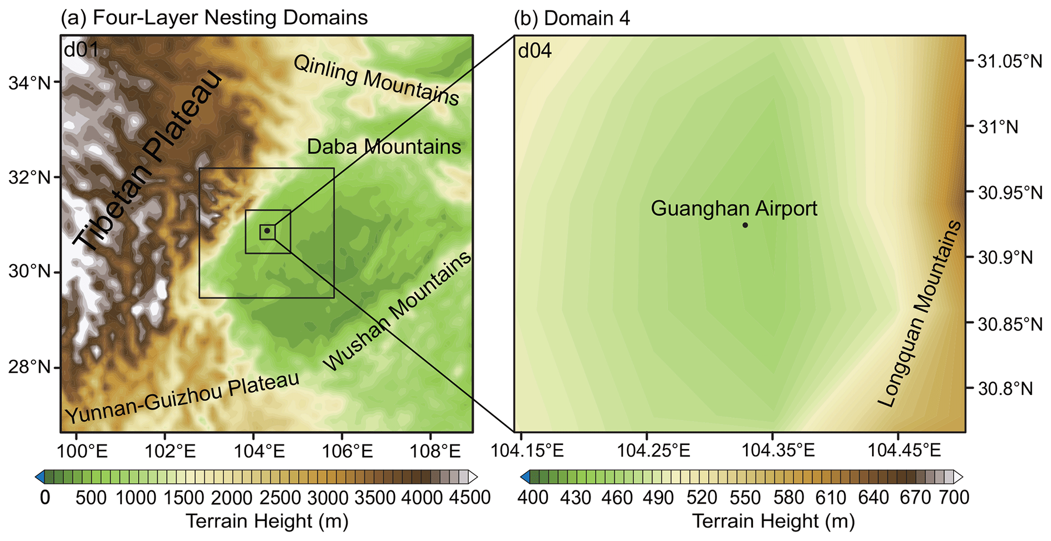
Figure 1 Configurations of (a) four-layer nesting domains (D01–D04) in WRF and the (b) study area. The spatial resolutions are 9, 3, 1, and 0.3 km for domains D1 to D4, respectively. The figure depicts the actual orography implemented in the experiments.

Given the complex terrain in the study region and the high resolution of the model design, the input of land surface data is particularly important, and its accuracy will directly affect the simulation of land surface processes and atmospheric boundary layer characteristics (Qi et al., 2021). Therefore, we replaced the terrain data of the four-layer nested area with 3 s resolution (∼90 m) from the southwest region of the Shuttle Radar Topography Mission v3 (SRTM3) (Farr et al., 2007).

To evaluate the model's ability in different PBL schemes, the observed wind fields at 10 m height at Guanghan Airport station are used. The terrain here is flat and homogeneous, and the prevailing wind directions are north and northeast in climatology. Wind direction and speed were measured using a first-class three-cup anemometer and wind vane, both manufactured by Thies Clima Inc. in Germany. The anemometer has a measurement range of 0.3 to 75 m s⁻¹ and a starting threshold of less than 0.3 m s⁻¹, with an accuracy of 1 % of the measured value or less than 0.2 m s⁻¹. The wind vane covers a measurement range of 0 to 360°, with a starting threshold of less than 0.5 m s⁻¹ at a 10° amplitude (as per ASTM D 5366-96) and 0.2 m s⁻¹ at a 90° amplitude (according to VDI 3786 Part 2) and an accuracy of 0.5°. During the research period, the anemometers were annually calibrated by accredited institutions. Before incorporating the wind data into our analysis, we performed basic data checks and quality-control procedures, including outlier removal.

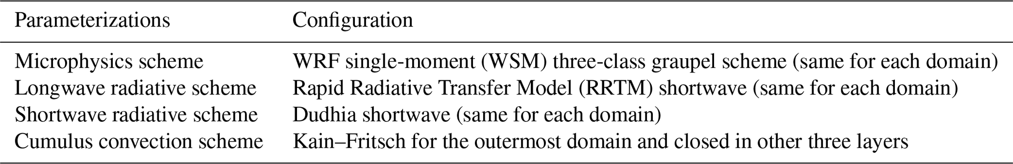
The hourly reanalysis ERA5 dataset with a horizontal resolution of 0.25° and 38 vertical levels is used to provide the initial and boundary conditions for WRF simulations, which are updated every 3 h when input into the model. Each event is simulated using four different PBL parameterization schemes. Thus, a total of 112 simulations is carried out. Each simulation spans 24 h, with the corresponding high winds in the middle of the simulation, discarding a spin-up period of 3 h. The model results are output every 10 min, enabling a high temporal resolution for demanding airport support operations, and the other model configuration is summarized in Table 1.

Table 1 Configuration of the physics scheme in the WRF simulation.

2.2 PBL schemes

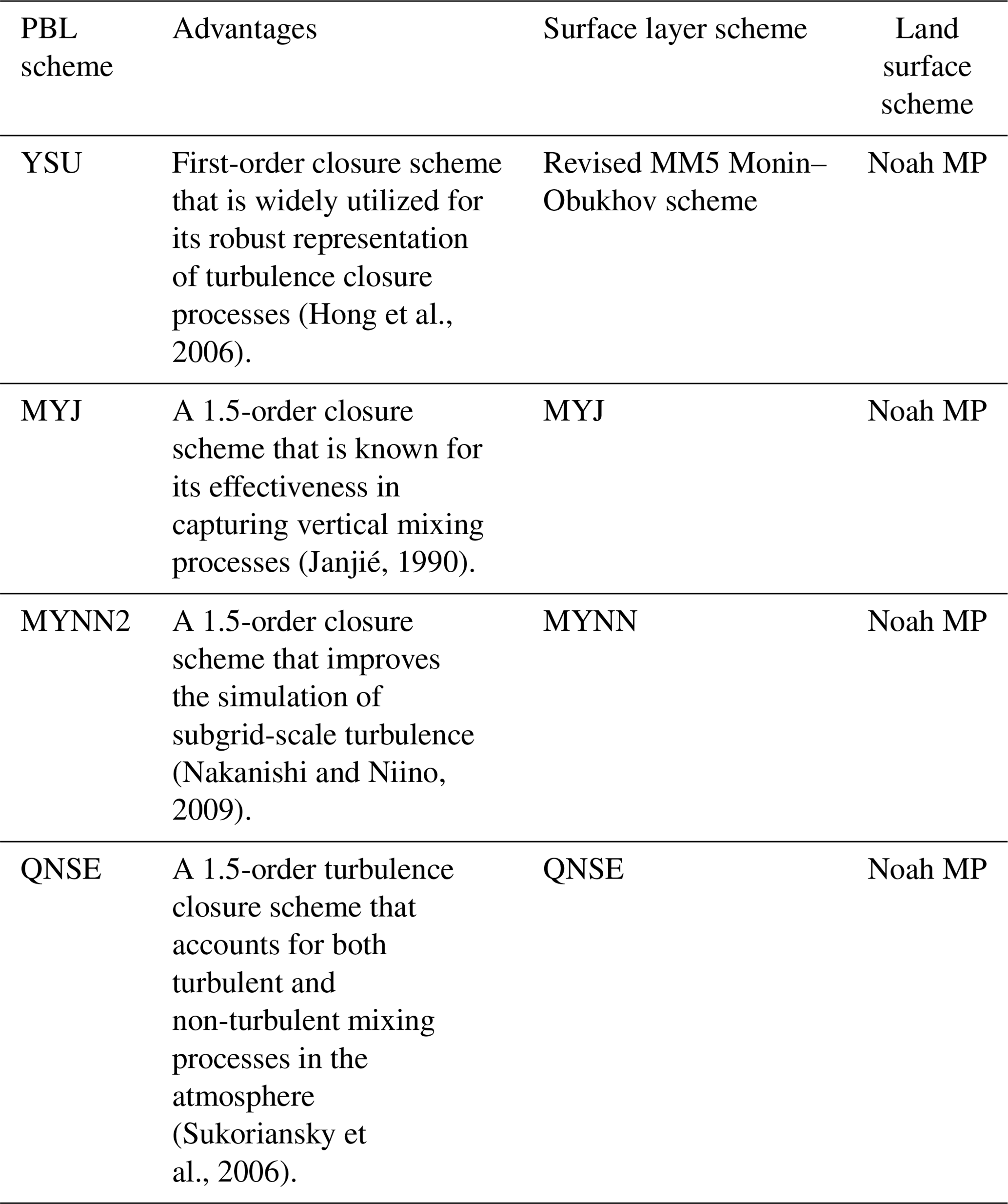
There are more than 10 PBL parameterization schemes in WRF v4.3.1, but four commonly used PBL schemes were selected for this study, namely the Yonsei University (YSU) scheme (Hong et al., 2006), the Mellor–Yamada–Janjić (MYJ) scheme (Janjié, 1990), the Mellor–Yamada–Nakanishi–Niino level 2 (MYNN2) scheme (Nakanishi and Niino, 2009), and the quasi-normal scale elimination (QNSE) scheme (Sukoriansky et al., 2006). Among them, YSU is a non-local, first-order closure scheme that represents entrainment at the top of the PBL explicitly, while the rest are local closure schemes. In-detail characteristics can be seen in Table 2. The surface layer scheme in the experiment is matched with each PBL scheme.

Table 2 The four selected PBL schemes and surface schemes in the experiment.

2.3 Statistical metrics for validation

As suggested by Wang et al. (2017), different sky conditions and atmospheric stabilities will affect the simulation of wind fields. Therefore, in order to accurately evaluate the sensitivity of the four PBL schemes to the near-surface wind field in the western Sichuan Basin on the east side of the Qinghai–Tibet Plateau, 28 near-surface wind cases are selected for the simulation based on wind speed data at 10 min intervals from 2021 to 2022, when the 10 min averaged wind speeds greater than or equal to 6 m s⁻¹ last for 30 min, and the result is evaluated separately through different circulation patterns and a k-means clustering analysis method. The main statistical metrics used include the following.

Root mean square error (RMSE) is the square root of the average of the squared differences between the simulated and observed values. RMSE is a commonly used metric in model evaluation, assigning higher weight to cases with larger simulation errors:

$$\begin{array}{}\text{(1)}& \mathrm{RMSE}=\sqrt{{\displaystyle \frac{\sum _{i=\mathrm{1}}^N{\left(O_i-S_i\right)}^{\mathrm{2}}}{N}}},\end{array}$$

where N is the total number of samples, O_i represents the observed near-surface wind, and S_i denotes the simulated near-surface wind, measured in m s⁻¹.

The correlation coefficient (COR) is an indicator that measures the strength and direction of the linear relationship between simulations and observations. By analyzing COR, the consistency between simulation results and observation results can be evaluated, and the corresponding PBL scheme can accurately capture the variation relationship of ground wind speed:

$$\begin{array}{}\text{(2)}& \mathrm{COR}={\displaystyle \frac{\sum _{i=\mathrm{1}}^N\left(s_i-\stackrel{\mathrm{‾}}{s}\right)\left(O_i-\stackrel{\mathrm{‾}}{O}\right)}{\sqrt{\sum _{i=\mathrm{1}}^N{\left(s_i-\stackrel{\mathrm{‾}}{s}\right)}^{\mathrm{2}}\sum _{i=\mathrm{1}}^N{\left(O_i-\stackrel{\mathrm{‾}}{O}\right)}^{\mathrm{2}}}}},\end{array}$$

where N is the total number of samples, O_i represents the observed values, and S_i denotes the simulated values.

Bias refers to the average difference between simulated and observed values, reflecting the overall bias of the simulation results. If bias is close to 0, it indicates that the simulation results have good accuracy at the average level. The calculation formula is as follows:

$$\begin{array}{}\text{(3)}& \mathrm{BIAS}={\displaystyle \frac{\mathrm{1}}{N}}\sum _{i=\mathrm{1}}^N\left(S_i-O_i\right).\end{array}$$

The Weibull distribution is a probability function used to describe the distribution of wind speed (Lai et al., 2006; Jiang et al., 2015). The expression for the Weibull distribution probability density function of wind speed v is

$$\begin{array}{}\text{(4)}& f\left(\mathit{\nu }\right)={\displaystyle \frac{\mathit{\kappa }}{\mathit{\lambda }}}{\left({\displaystyle \frac{\mathit{\nu }}{\mathit{\lambda }}}\right)}^{\mathit{\kappa }-\mathrm{1}}\exp \left[-{\left({\displaystyle \frac{\mathit{\nu }}{\mathit{\lambda }}}\right)}^{\mathit{\kappa }}\right],\end{array}$$

where k is the shape parameter, a dimensionless parameter, and λ is the scale factor, measured in m s⁻¹. These two parameters can be calculated using the following formulas:

$$\begin{array}{}\text{(5)}& {\displaystyle }& {\displaystyle }\mathit{\kappa }={\displaystyle \frac{\mathit{\sigma }}{\mathit{\mu }}},\text{(6)}& {\displaystyle }& {\displaystyle }\mathit{\lambda }={\displaystyle \frac{\mathit{\mu }}{{\left(\mathrm{0.568}+\frac{\mathrm{0.434}}{k}\right)}^{\frac{\mathrm{1}}{k}}}},\end{array}$$

where σ and μ represent the standard deviation and mean value of the wind speed, respectively.

3 Overview of historical cases and evaluation of simulation results

3.1 Summary of 28 near-surface wind events

Since the experimental approach consists of multiple case simulations in this study, it is necessary to understand the characteristics of these cases, such as the temporal variation, the peak time, and synoptic factors, which can help to classify them and evaluate their simulation performance separately in the following analysis.

Therefore, Table 3 provides detailed information derived from wind data recorded at 10 min intervals. It is shown that out of the 28 near-surface wind events participating in the simulation, 24 were northerly events, accounting for 85 % of the total. The events in which the maximum wind is above 8 m s⁻¹ account for 18 %, and the events of 5–7 m s⁻¹ account for 82 %. Meanwhile, the wind direction corresponding to the peak time was distributed between 350–50°, with northeasterly winds between 0–50° being the most common. Additionally, those remaining are four southerly winds cases, all of which appear to occur in summer or early autumn.

Table 3 Characteristics and circulation patterns of the 28 chosen near-surface wind events.

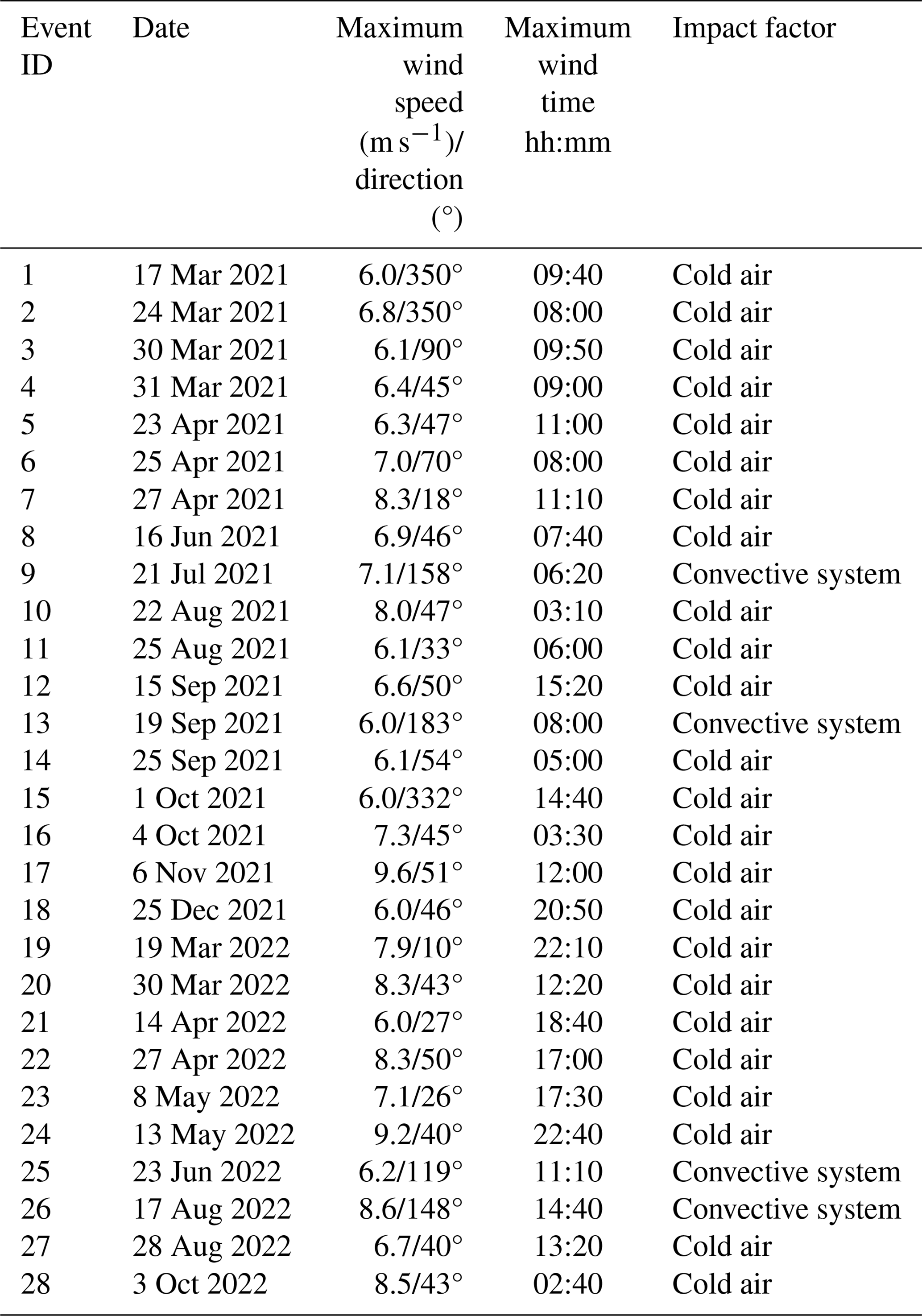
As for the dominating factors of each event, the term cold air in Table 3 is used to denote the cases which are generated by incursion of cold air from northern regions like Siberia or Mongolia in the Sichuan Basin, often accompanied by sharp temperature drops and changes in humidity. The term convective system specifically denotes the strong wind cases primarily caused by convective weather systems, often accompanied by thunderstorms. In such cases, vertical motion or convection is the dominant factor. It is shown that most of the wind events were mainly caused by incursion of cold air, and few were associated with convective weather systems. Influenced by this, the spring (March–May) process accounted for the most, accounting for 46 %, followed by summer and autumn, both accounting for 25 %. In terms of the peak time, 60 % of the simulated cases appear to concentrate between 17:00–21:00 and 22:00–02:00 UTC at night, followed by 15:00–19:00 UTC, and there are a total of six events that occurred at 20:00–23:00 and 00:00–04:00 UTC, accounting for 21 %.

The near-surface wind speed in the Sichuan Basin exhibits a distinct diurnal variation, characterized by lower wind speeds in the morning and evening and higher wind speeds at midday. In order to analyze the temporal variation in wind speed under different conditions, the hourly time series of the observed wind speed for 28 cases is presented in Fig. 2. It is shown that many cases with the incursion of cold air exhibit diurnal variation characteristics because, in these cases, cold air predominantly affects the western Sichuan Basin around midday (Table 3). However, for strong wind events, such as case nos. 9, 13, 25, and 26, which are caused by convective systems, there is no clear diurnal variation in wind speed, and they are characterized by sudden changes in wind speed, reflecting the transient and localized nature of convective processes.

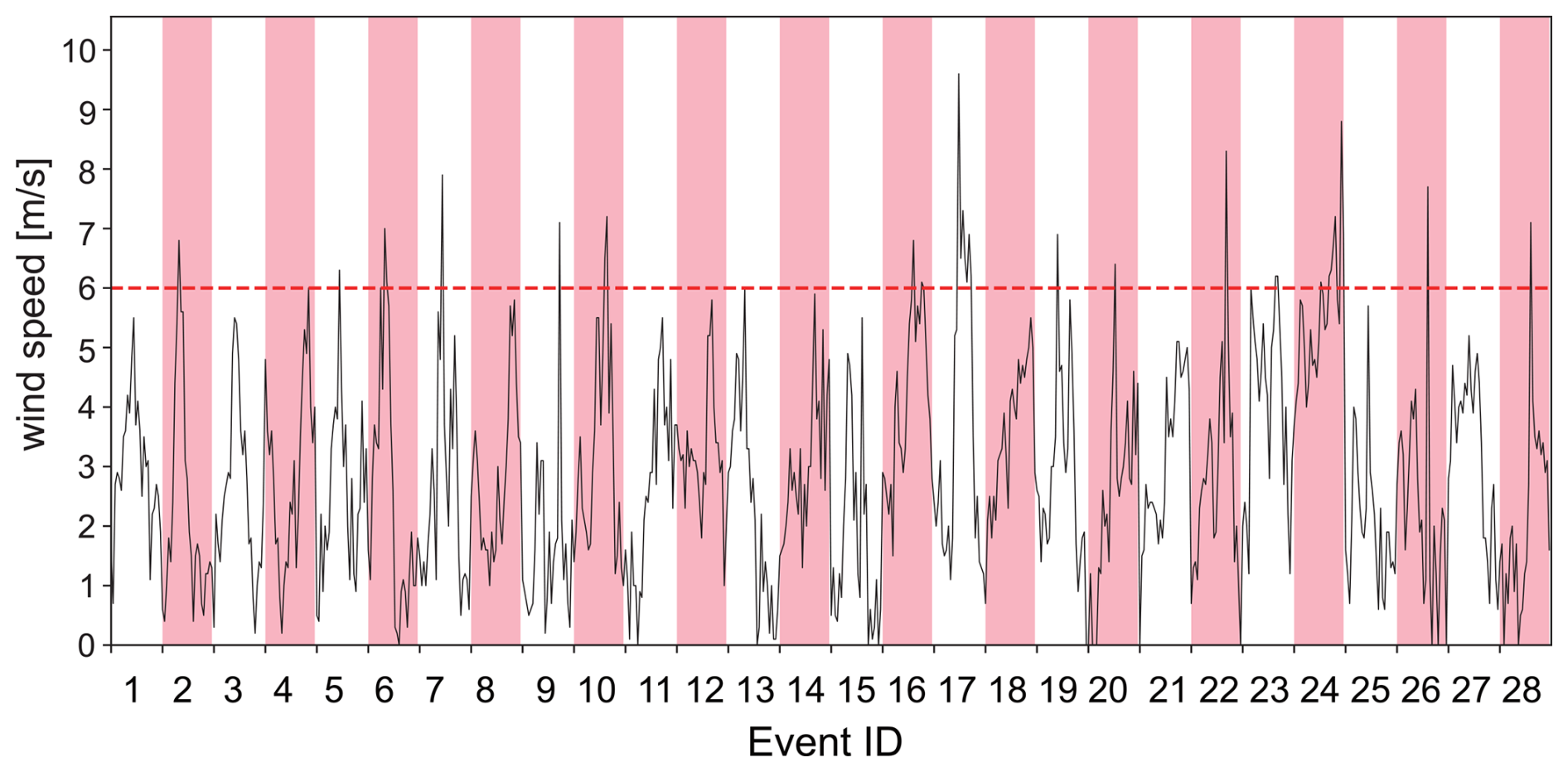
Figure 2 The time series of hourly wind speed for all 28 near-surface wind events listed in Table 3. Each event represents 1 d, the label of the x axis represents the event ID shown in Table 3, and the shading is employed to distinguish the time series of the 28 selected cases, which are discontinuous across days.

3.2 Overall simulation performance of 28 wind events

First, the performance of the model in different PBL schemes is assessed with respect to wind direction. Thereby, the simulated wind roses of the four PBL schemes are given in Fig. 3. By comparing with the observation (Fig. 2), it is found that the four PBL schemes can reproduce the distribution of wind direction. Specifically, the simulated wind directions are basically distributed in the NNW, N, NNE, NE, and ENE directions, reproducing the characteristics of highly concentrating on NNE and NE. Moreover, it is also shown that the occurrence frequencies of the wind fields simulated by all PBL schemes in the NNE and NE directions are all relatively higher than those of the observations, but for wind in the NNW direction, the simulated frequencies are significantly lower, indicating a clockwise bias that may be related to the plateau topography with steep terrain in the northwest and west. The statistical metrics (Gómez-Navarro et al., 2015) in the simulated 10 m wind direction are also given in Table 4. From the perspective of bias, RMSE, and circular COR, the differences in the wind directions among the four PBL schemes are relatively small. However, these differences are not negligible and suggest that while the impact of different PBL schemes on wind direction is minor, it is observable. Therefore, it can be inferred that the wind direction of the near-surface wind field in the western Sichuan Basin shows some sensitivity to the selected PBL scheme, though the variations are moderate.

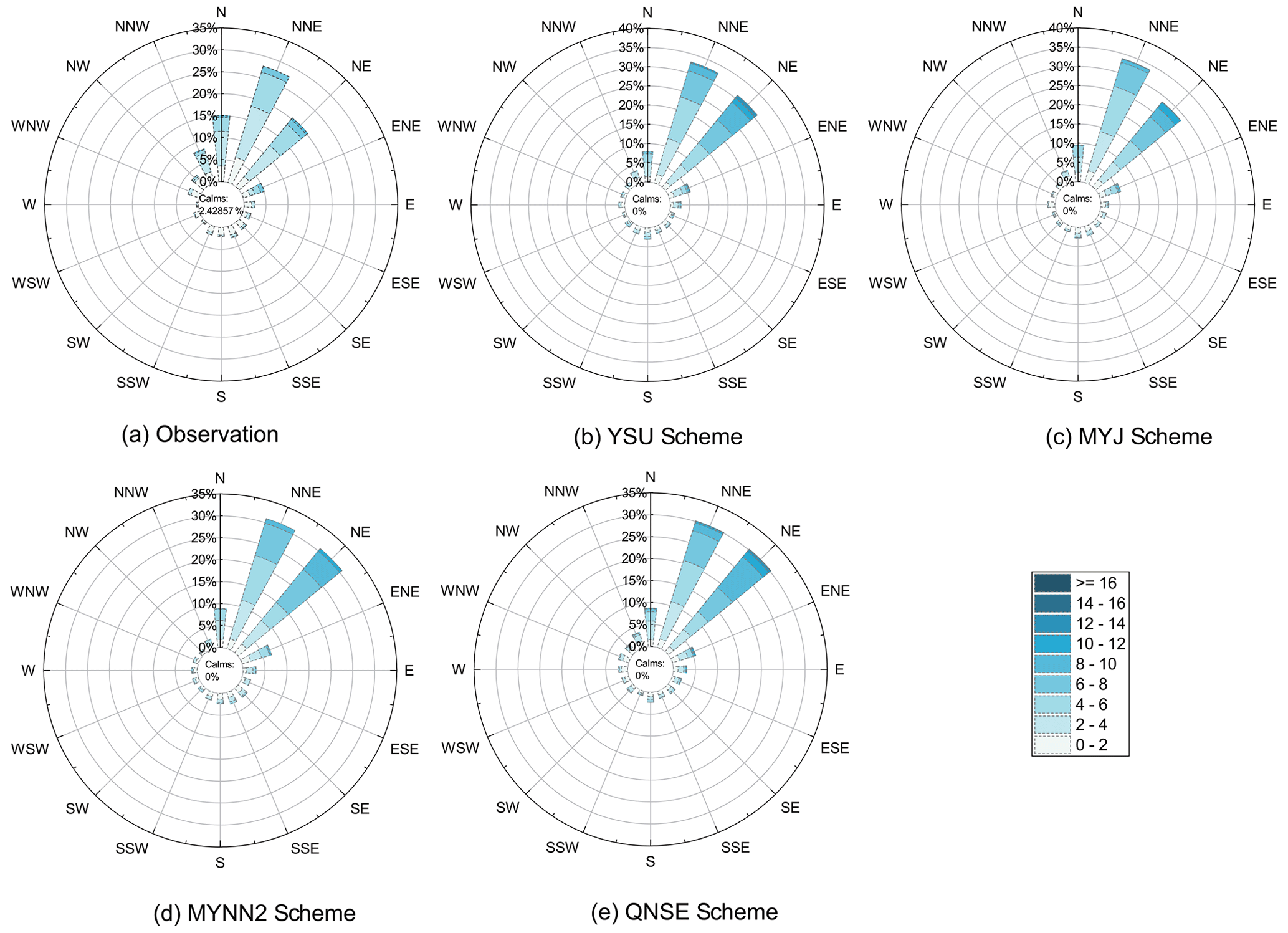
Figure 3 The wind rose chart for all the observed and simulated 28 near-surface wind events listed in Table 3, (a) for observations, (b) the YSU scheme, (c) the MYJ scheme, (d) the MYNN2 scheme, and (e) the QNSE scheme. The circles represent the relative frequency (%), and the colors represent wind speed.

Table 4 Statistical metrics for simulated 10 m wind direction.

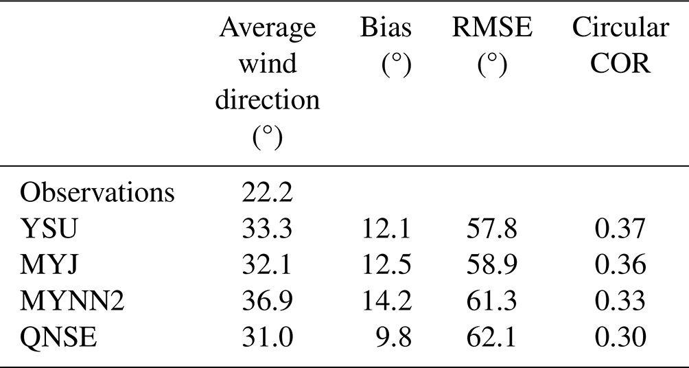
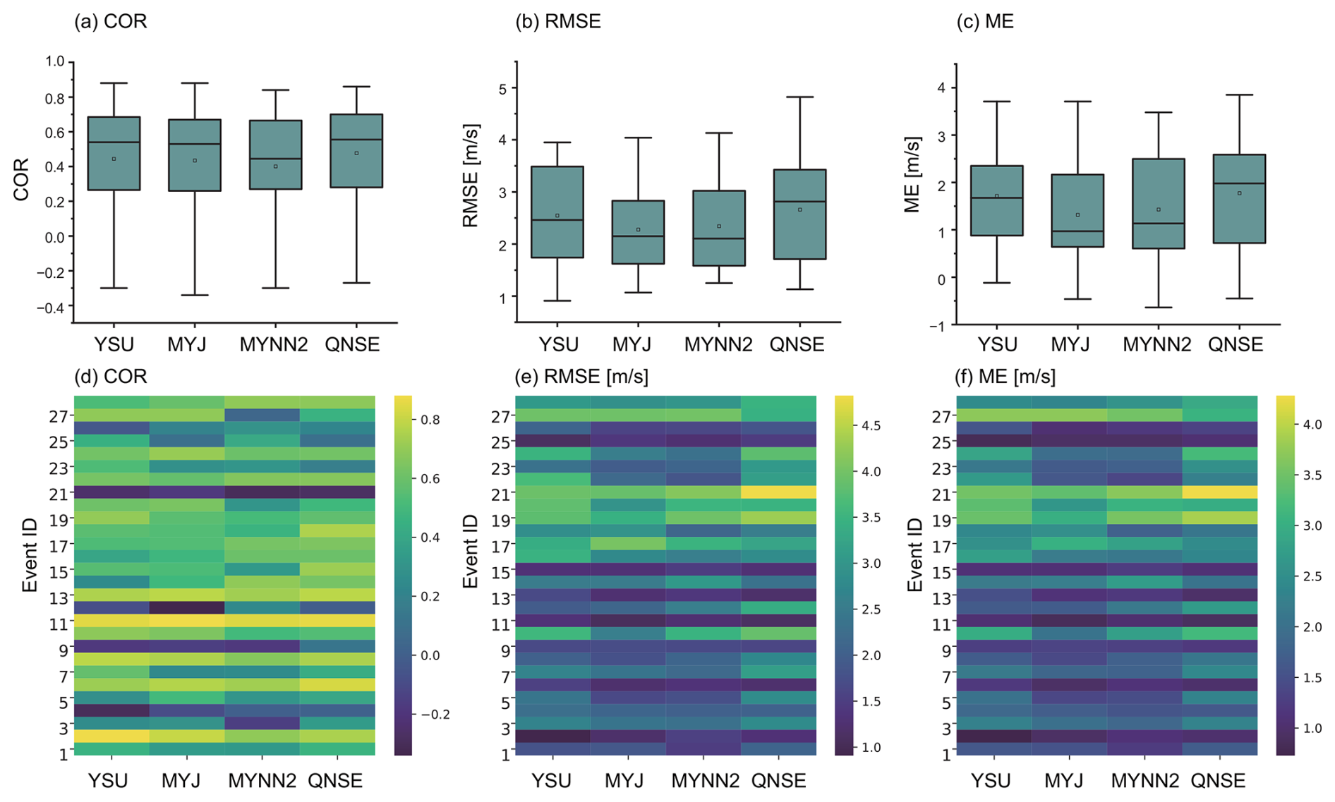
Figure 4 Different performance metrics for the comparison of observed and simulated near-surface wind speed at 10 min intervals for the 28 events. Box plots show the overall characteristics of COR, RMSE, and bias, and the heatmap gives details for certain cases. The box represents the metric range from the first quartile to the third quartile, and the line inside the box represents the median, while the empty square represents the mean.

However, there are still some differences in the wind direction simulations among the four PBL schemes. In the MYJ scheme, the frequency of NNE wind is higher than that of NE wind, which is consistent with the observations. Moreover, the frequencies of N wind and NE wind are closer to the observations. Therefore, MYJ has the best simulation of wind direction. The wind direction distribution simulated by the MYNN2 scheme is very close to that of the QNSE scheme, but due to the worse performance in simulating NNW wind and the larger frequency of simulated NNE and NE winds, the MYNN2 scheme is the worst among the four schemes. In general, for wind fields with weather processes passing through, more attention is paid to the simulation of wind speed. Therefore, we focus on the performance of wind speed next.

In fact, by comparing Figs. 2 and 3, it seems that all four PBL schemes exhibit obvious exaggeration of wind speed, which is also shown in numerous other studies (Dzebre and Muyiwa, 2020; Ma et al., 2024). For instance, in the research by Yu et al. (2022), all 11 WRF PBL schemes overestimate near-surface wind speeds by approximately 1 m s⁻¹ in the Hebei Plain. Similarly, in the experiment conducted by Gómez-Navarro et al. (2015), the MYJ scheme strongly overestimates the maximum wind speed by more than 10 m s⁻¹ at 50 % of the locations, while the YSU scheme shows deviations greater than 3 m s⁻¹. But what are the specific simulation characteristics of these commonly used PBL schemes in the Sichuan Basin? To further evaluate the advantages and disadvantages of each scheme in simulating near-surface wind speed, three statistical metrics (COR, RMSE, and bias) were calculated. These statistics were derived from data recorded at 10 min intervals across 28 distinct events, as illustrated in Fig. 4. In terms of COR, both the mean and the median values for all schemes fall within the range of 0.4 to 0.6, which indicates a tendency for the COR to cluster around this range across the events. Moreover, the median is above the mean value, indicating that the correlation coefficients all have a negatively skewed distribution; that is, the correlation coefficients between the simulated and observed wind speeds are higher than the mean value in most cases but very poor in some cases. This is further illustrated by the heatmap displayed in Fig. 4d, where case nos. 3, 11, and 20 demonstrate correlation coefficients below 0. In contrast, QNSE shows the best mean correlation coefficient of 0.6, suggesting the best performance in reproducing the temporal variation in observed wind speed in most cases.

Although there is little difference between the simulated and the observed wind speeds in the RMSE and bias, it is noteworthy that the MYJ scheme has the smallest mean RMSE and bias (2.3 and 1.2 m s⁻¹), while QNSE has the largest (2.7 and 1.8 m s⁻¹). The bias is consistent with the RMSE, as illustrated in Fig. 4c, except that the median and mean bias is not as close as the RMSE shows in the MYJ scheme, indicating that the systematic error (bias) might be either too high or too low in certain cases. However, overall, the MYJ scheme is highly precise and has little variance in its performance, which is crucial for accurate weather forecasts. The main reason for this may be associated with the basin topography. Because the boundary layer is in a stable condition most of the time, the turbulence is mainly generated and maintained by wind shear so that the situation shows strong locality. Therefore, the simulation error obtained by the MYJ scheme is the smallest in this stable and weakly stable boundary layer, which is consistent with the research results of Zhang et al. (2012). Moreover, the result that the QNSE scheme has the best performance in capturing the temporal variation in wind speed may be because it improves the simulation of subgrid-scale turbulence and considers more complex and detailed physical processes. Under stable atmospheric stratification, QNSE adopted a k–ε model developed from a turbulent spectral closure model, while in the unstable situation, the method of the MYJ scheme is used, so the QNSE scheme has more advantages in the simulation of the wind speed variation trend. However, the specific causes require further investigation in future works.

3.3 Differences in wind velocity segments and diurnal variations simulated by the four PBL schemes

Figure 5 shows the frequency distribution of different winds with the observed and the simulated wind data at Guanghan Airport. As can be seen, the observed wind speed distribution is left skewed, primarily due to the concentration of wind speeds within the 1–4 m s⁻¹ range, where the cumulative frequency exceeds 0.6. When comparing the spread of each PBL scheme's distribution to the observations, all four PBL schemes exhibit a wider distribution, indicating overestimation of the wind speed variability.

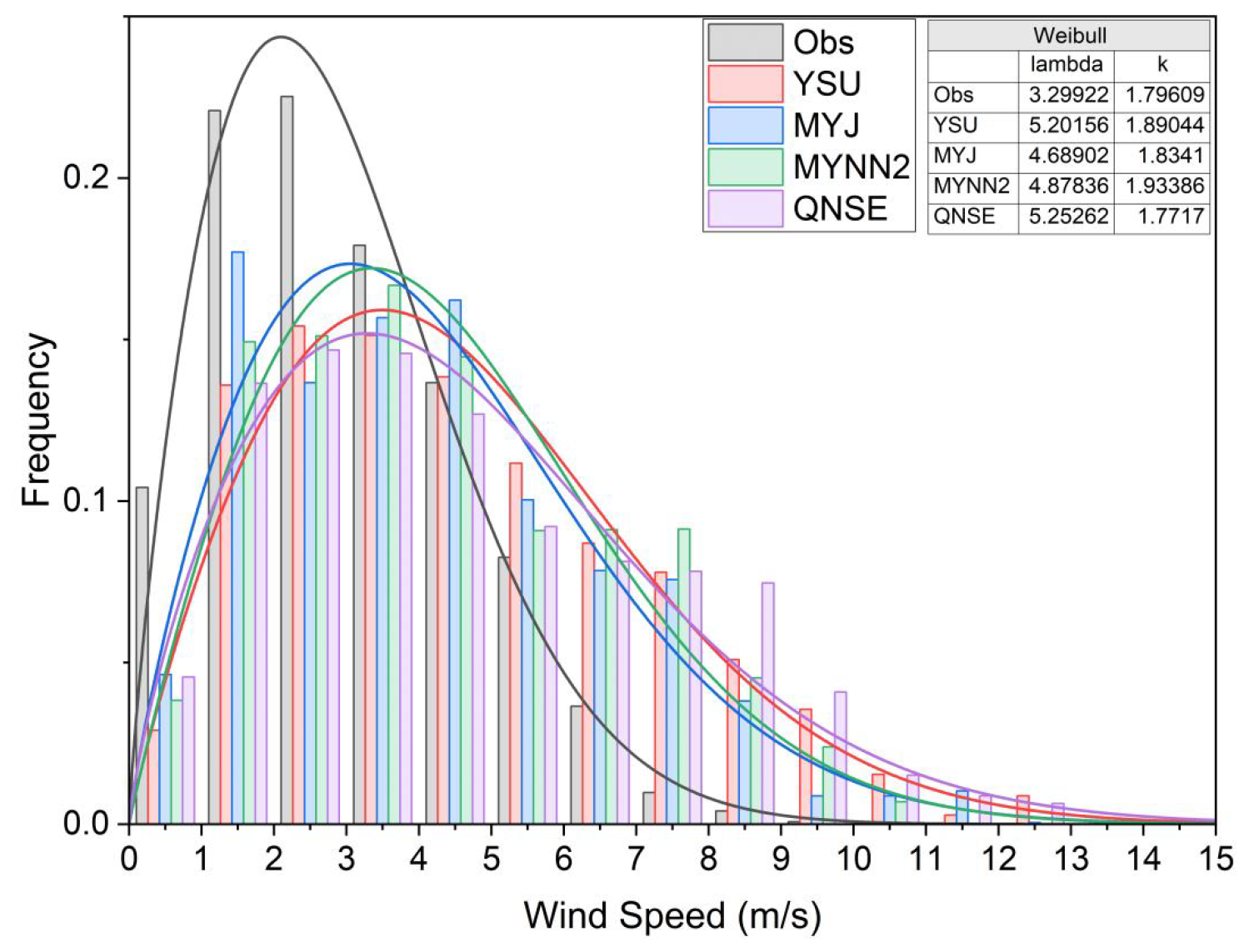
Figure 5 The frequency distribution of different wind speeds and Weibull fitting curves for the observed and simulated wind speeds from the four PBL schemes, sampled every 10 min during 28 wind events. The shape parameter is denoted by k and the scale parameter by λ. Each colored line and bar represents one of the PBL schemes.

In order to quantitatively compare the performance of the four PBL schemes, a Weibull distribution fitting was applied in Fig. 5. The shape parameter (k) represents the concentration of the wind speed distribution. A lower k value indicates a more dispersed distribution with greater wind speed variability, while a higher k value suggests a more concentrated distribution with less variability. The observed k value is 1.79, while the shape parameters for YSU, MYJ, MYNN2, and QNSE are 1.89, 1.83, 1.93, and 1.77, respectively. With a shape parameter of 1.77, QNSE is closest to the observed value, indicating that it captures the variability of wind speeds more effectively than the other schemes. Therefore, from a shape parameter perspective, QNSE provides the most similar wind speed distribution to the observations. Conversely, YSU and MYNN2 yield higher k values, suggesting a more concentrated distribution that underestimates variability.

The scale parameter λ, representing the spread of wind speeds, shows systematic overestimation for all PBL schemes. The observed λ is 3.30 m s⁻¹, while the scale parameters for YSU, MYJ, MYNN2, and QNSE are 5.20, 4.69, 4.88, and 5.25 m s⁻¹, respectively. Therefore, MYJ and MYNN2 exhibit smaller deviations in λ, indicating closer alignment with observed wind speeds, whereas YSU and QNSE show the largest overestimation.

The performance of the PBL schemes varies across different wind speed ranges. When the wind speed is below 3 m s⁻¹, none of the PBL schemes show good performance, and the lower the wind speed, the greater the bias. In the wind speed range of 3–5 m s⁻¹, different PBL schemes show significant differences compared with observations. Specifically for wind speeds between 3–4 m s⁻¹, the simulation results of the MYJ scheme are closest to the observations, followed by MYNN2. For wind speeds between 4–5 m s⁻¹, YSU and MYJ simulations are closer to the observations, indicating better performance in this wind speed range. All schemes tend to overestimate when wind speed is above 5 m s⁻¹. Figure 6 further provides the deviations between the observed and simulated wind speeds of the four PBL schemes in different wind speed ranges. As can be seen, the performance of the four PBL schemes differs greatly with an increase in wind speed, and the wind speed deviation of the same PBL schemes also increases. For the wind speed below 3 m s⁻¹, the simulated wind of each PBL scheme is about 1.5–2 m s⁻¹ higher than that of the observations. In terms of mean values, the MYJ scheme exhibits relatively smaller deviations for wind speeds below 8 m s⁻¹, an average deviation ranging from 0.5 to 1.25 m s⁻¹. In contrast, for wind speeds above 8 m s⁻¹, the MYNN2 scheme demonstrates the smallest deviation, with an average deviation of 2 m s⁻¹.

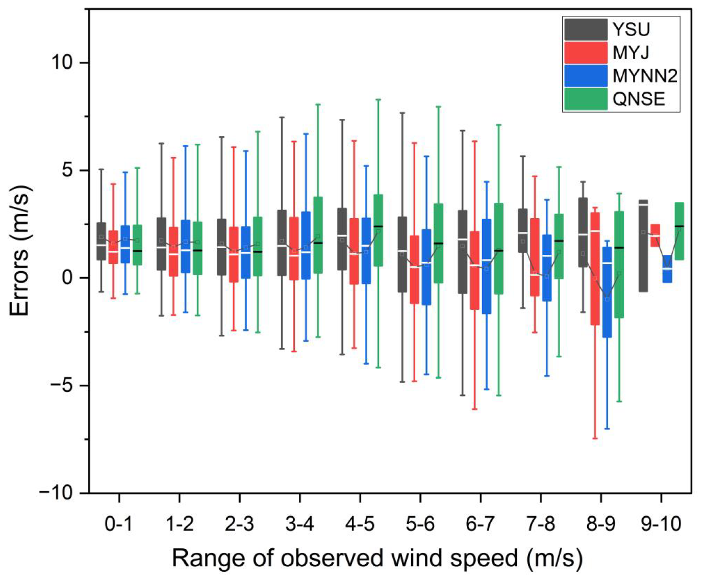
Figure 6 Wind speed errors of the four PBL schemes in different wind speed segments for 28 wind events with 10 min intervals. The line inside the box represents the median.

In general, the fitting curve of the QNSE scheme is closest to the observation, and the λ value is slightly to the right of the mode. However, it is critical to highlight that the MYJ scheme matches observations better than the other schemes in terms of wind speed. As shown in both Fig. 5 and Fig. 6, the MYJ scheme consistently exhibits a lower error across various wind speed ranges and aligns more closely with the observed frequency distribution. While all schemes show modes to the right of the observed wind speed distribution, the MYJ scheme demonstrates a performance that is closest to the observed data, indicating a tendency towards a more accurate representation of wind speeds.

The variation in the near-surface wind field is easily affected by surface characteristics, especially ground heating. When the weather background is fixed, the change in local thermal characteristics in a day will inevitably affect the near-surface wind field. Therefore, there will be significant differences in the wind field simulation during different time periods between different PBL schemes. In this study, since the study area is located in a time zone of UTC +8 (local time), the daytime and nighttime periods were defined in terms of coordinated universal time (UTC). Daytime corresponds to 00:00–10:00 UTC, and nighttime refers to 11:00 to 23:00 UTC. Figure 7 presents the diurnal variation characteristics of wind speed deviations simulated by the four PBL schemes in the WRF model through box plots.

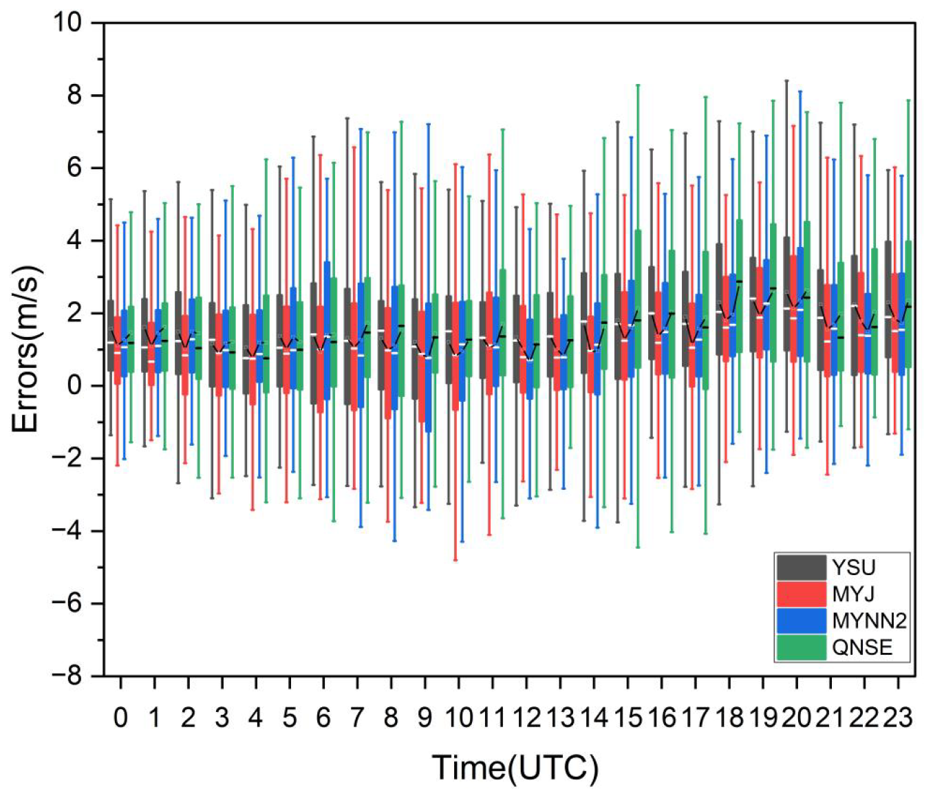
Figure 7 Diurnal variation in wind speed errors corresponding to the four PBL schemes. The line inside the box represents the mean, while the short black line connects the mean values of each PBL scheme at each hour. Statistics are derived from the data at 10 min intervals.

In terms of the mean, the performance of each scheme in simulating wind speed tends to be better during the daytime than at night. During the daytime, the MYJ scheme performs relatively well, particularly around local noon at 16:00 UTC, where the errors are the lowest (0.76 m s⁻¹), indicating that this scheme provides more stable and reliable simulations during this period. The highest deviations are observed at 18:00 UTC (with errors peaking at 2.80 m s⁻¹, followed by 19:00 and 20:00 UTC (2.62–2.63 m s⁻¹), indicating that the strong winds occurring during these times are not well simulated by any of the schemes. For the YSU scheme (gray color), the simulation capability is best around local noon (16:00 UTC), indicated by relatively lower mean errors of 1.02 m s⁻¹. This suggests that the YSU scheme effectively captures wind speed closer to local noon. The MYJ scheme (red color) shows reliable performance both at noon and in the evening, with errors ranging between 0.75–1 m s⁻¹, indicating robust simulation during these periods. The MYNN2 scheme (blue color) performs similarly well in the evening, with the lowest mean errors of 0.66 m s⁻¹ at 12:00 UTC. The QNSE scheme (green color), although showing little variation during the daytime, also demonstrates its best performance at noon with minimal mean errors of 1.18 m s⁻¹ (16:00 UTC). This consistent daytime performance suggests reliable outputs for various strong wind events during this period. However, the QNSE scheme exhibits increased variability during nighttime simulations, with errors varying more significantly.

In summary, the performance of the PBL schemes varies based on the time of the day, indicating that they may be sensitive to diurnal changes in atmospheric conditions. Each PBL scheme displays distinct performance characteristics, with the MYJ scheme showing particularly consistent and reliable performance during the daytime, especially around local noon (16:00 UTC), where the mean error is minimized.

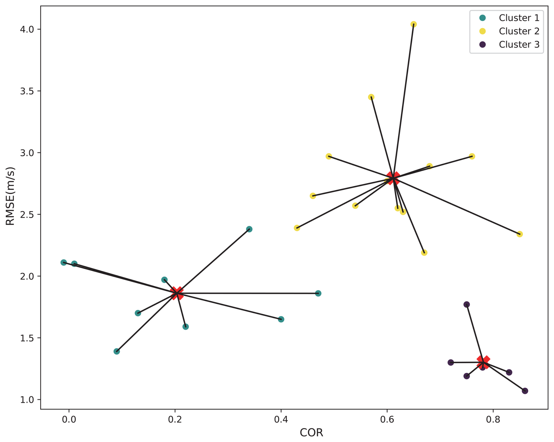
Figure 8 Scatter plot of k-means cluster analysis. The red cross symbol represents the cluster center.

3.4 K-means clustering analysis and performance in different types of events

From the previous analysis, it is known that as the horizontal grid spacing of 0.33 km is within the PBL gray zone resolution, the QNSE scheme can better capture the trend of near-surface wind events over the western Sichuan Basin, while the bias produced by the MYJ scheme is the minimum. The results also show differences across various wind speed ranges and different time periods in this region. Given the complexity of meteorological conditions in this area, the performance of different PBL schemes may vary under different circumstances. However, directly classifying cases based on weather conditions has not yielded clear insights, partly due to the large differences in sample sizes across categories (Table 3). Therefore, to more effectively evaluate the specific performance of the PBL schemes in simulating near-surface wind events, it is necessary to further classify the 28 cases based on model performance metrics, which can provide a more reliable and meaningful distinction of the schemes' capabilities.

The k-means cluster method based on the RMSE and COR of the four PBL schemes is used to divide the simulation results of the 28 near-surface wind events into three categories, as presented in Fig. 8. The RMSE of the cluster center of the first class is 1.9 m s⁻¹, and the COR is 0.2. A total of 10 events belongs to this class, characterized by moderate RMSE but poor COR. For the second class, the cluster center has an RMSE of 2.85 m s⁻¹ and a COR of 0.6. This class includes 12 events, indicating higher RMSE but better COR. The remaining six events fall into the third category, where both RMSE and COR are optimal for simulation. The cluster center for this class has an RMSE of 1.25 m s⁻¹ and a COR of 0.76.

Furthermore, it is shown that among these three categories, the QNSE scheme has the best simulation correlation coefficient, while the MYJ scheme has the smallest wind speed simulation error. This consistency in performance is in line with the results prior to applying k-means clustering, indicating that QNSE and MYJ schemes are relatively robust and reliable choices for the near-surface wind simulation in the western Sichuan Basin with a model grid resolution of 0.3 km. Detailed information on the individual cases corresponding to each cluster can be found in Fig. 9.

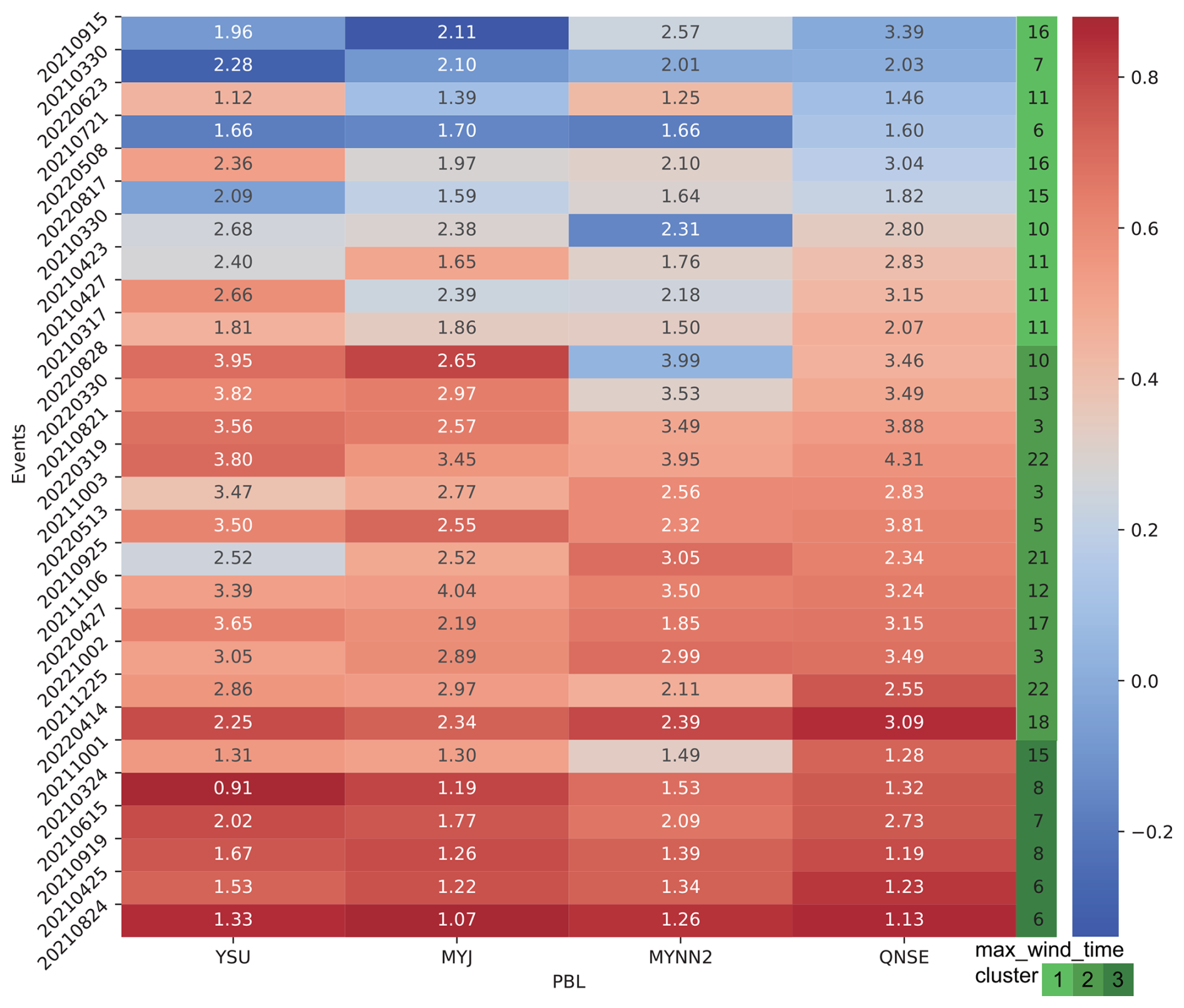
Figure 9 Heatmap of the RMSE (numbers) and COR (coloring) of the four PBL schemes for the 28 near-surface wind simulations according to the cluster analysis. The information in the right column is the gale moment (numbers) and classification label (coloring).

Figure 9 shows the RMSE and COR heatmaps of three types of events after cluster analysis, and the peak time of gales is specially marked. It is found that different PBL schemes are very sensitive to diurnal variation. The events in class III are characterized by the fact that the gale period basically occurs between 06:00 and 08:00 UTC, a period known for maximum surface temperatures and the most unstable atmospheric stratification during the day. This period is characterized by strong surface heating that drives convective turbulence, which leads to vertical mixing and relatively strong near-surface winds. This dynamic makes it easier for models to capture wind profiles accurately. Additionally, in the events of class III, except for one thunderstorm gale event, the rest are all typical strong cold-air-induced near-surface wind processes, which indicates that the four PBL schemes have good performance in simulating the typical strong cold-air wind event that occurred in the afternoon. As shown in Fig. 10, the RMSE ranges from 0.21 to 0.96 m s⁻¹, and the COR ranges from 0.05 to 0.19, with only one case having a difference of 0.3, which means that there is little difference between the four PBL schemes.

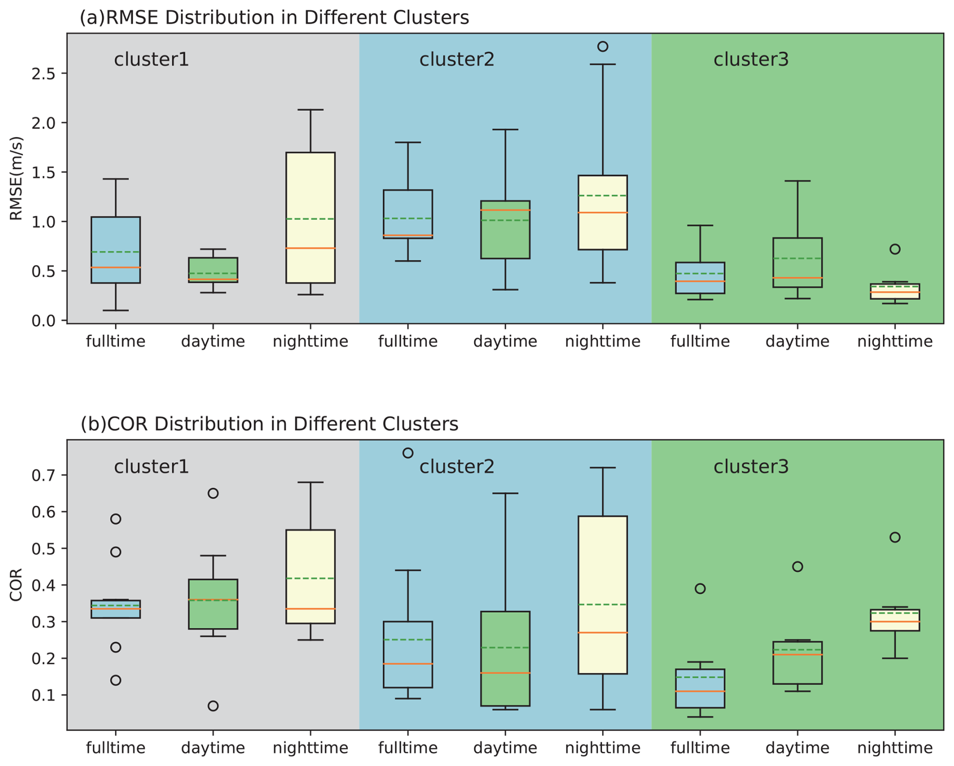
Figure 10 Box plots of the maximum differences during the four PBL schemes in three types of events, with the dotted green line showing the mean, the solid orange line the median, and the circle the outlier.

The most obvious differences among the four PBL schemes are mainly in the events of classes I and II. Except for one southerly gale event belonging to class III, the other southerly wind events are classified into class I, indicating that the four PBL schemes often have good RMSE and poor COR for southerly wind events, caused by convection in the western Sichuan Basin. In Fig. 9, it is shown that for class I, the maximum wind speeds most frequently occur during the two periods of 10:00–11:00 and 15:00–16:00 UTC, with only two cases occurring between 06:00–07:00 UTC. The period from 10:00 to 16:00 UTC corresponds to the transition of the atmospheric stratification in the basin from unstable to stable conditions, during which the inversion layer is established. For these events, the difference between the maximum and minimum RMSE and COR obtained by different PBL schemes is as large as 1.43 m s⁻¹ and 0.58, respectively.

The simulation events of class II exhibit the most significant differences among the four PBL schemes, with characteristics such as gale occurrence times differing markedly from those in class I and class III. It is observed that the four PBL schemes often display high correlation coefficients (CORs) and high RMSEs for near-surface wind events occurring in the early morning (05:00–10:00 UTC) and early afternoon (15:00–17:00 UTC). In the early morning in particular, the boundary layer typically experiences stable stratification due to radiative cooling, which suppresses vertical mixing, and near-surface winds weaken significantly, leading to the highest RMSE due to the models' inability to accurately simulate the disturbances and small-scale dynamics in this stable period. In this type of event, the maximum differences in RMSE and COR among the PBL schemes can reach 1.49 m s⁻¹ and 0.76, respectively. In addition, Fig. 10 shows that the differences between different PBL schemes in class I and class II events in the daytime are relatively small, while there are greater differences at night. Meanwhile, in class III, the RMSE performance at night is better than that in the daytime, but the COR is worse than that in the daytime. Therefore, it can be concluded that there are obvious and diversified differences among the simulation results shown by various PBL schemes under different types of near-surface wind events.

4 Summary and conclusions

In this study, a horizontal resolution of 0.33 km, which is within the PBL gray zone resolution, is employed to investigate the performance of four commonly used PBL schemes in near-surface wind simulation over the Sichuan Basin. In China, near-surface wind prediction over the Sichuan Basin always has a low score, and the main focus of wind simulation is on pollutant diffusion under stable weather conditions at a horizontal resolution equal to or greater than 1 km. Thus, we chose the site of Guanghan Airport as the representative area and conducted a total of 112 WRF sensitivity experiments, specifically focusing on 28 events with near-surface winds exceeding 6 m s⁻¹ by varying the PBL scheme, and we assessed the impact of different PBL schemes on wind speed and direction simulations. Subsequent analyses considered factors such as diurnal variation in near-surface wind processes and circulation background to gain further understanding of their influence on model sensitivity. Therefore, the findings of our study offer valuable insights into this region.

From our evaluation and analysis, it was found that the sensitivity of near-surface wind direction over the Sichuan Basin to the four commonly used PBL schemes is very low, and the performance of MYNN2 is the worst when simulating the near-surface wind direction, while the other three schemes are generally consistent with observations, and the MYJ scheme is the best for simulating NNE and NE winds. Our findings on wind direction agree with those in many other research works (Gómez-Navarro et al., 2015; Tan et al., 2017; Shen and Du, 2023).

Generally speaking, no scheme can simulate the trend and wind speed of near-surface wind events well at the same time, which is also mentioned by Cohen et al. (2015). However, the 1.5-order QNSE local closure approximation scheme appears to be the best for the temporal variation, while MYJ is the scheme with the smallest simulation error in wind speed. As the metrics RMSE and bias show similar characteristics, k-means cluster analysis is employed based on the COR and RMSE, and the simulation results are divided into three categories. The first category of events showed poor correlation but small RMSE, the second category of events showed high correlation but large RMSE, and the third category of events showed high correlation and small RMSE. Further analysis found that the four PBL schemes can simulate the ground wind events caused by the typical strong cold air (occurring at 06:00–08:00 UTC), and there is little difference between them. The near-surface wind events occurring from midnight to early morning are mainly concentrated in the second category, while the evening to night and the southerly wind process are mainly concentrated in the first category.

Therefore, multiple case studies and k-means clustering analysis give us an indication that the simulation performance of the PBL schemes mainly depends on the prevailing weather conditions of each case, such as circulation backgrounds and the time of near-surface wind events. The results also point to the need for future research to explore the mechanisms behind the observed differences in wind speed simulations, particularly during nighttime and different atmospheric conditions.