CitcomSVE-3.0: a three-dimensional finite-element software package for modeling load-induced deformation and glacial isostatic adjustment for an Earth with a viscoelastic and compressible mantle

Earth and other terrestrial and icy planetary bodies deform viscoelastically under various forces. Numerical modeling plays a critical role in understanding the nature of various dynamic deformation processes. This article introduces a newly developed open-source package, CitcomSVE-3.0, which efficiently solves the viscoelastic deformation of planetary bodies. Based on its predecessor, CitcomSVE-2.1, CitcomSVE-3.0 is updated to account for three-dimensional elastic compressibility and depth-dependent density, which are particularly important in modeling horizontal displacement for viscoelastic deformation. We benchmark CitcomSVE-3.0 against a semi-analytical code for two types of loading problems: (1) single harmonic loads on the surface or as a tidal force and (2) the glacial isostatic adjustment (GIA) problem with a realistic ice sheet loading history (ICE-6G_D) and an updated version of sea level equations. The benchmark results presented here demonstrate the accuracy and efficiency of this package. CitcomSVE-3.0 shows second-order accuracy in terms of spatial resolution. For typical GIA modeling with a 122 kyr glaciation–deglaciation history, a surface horizontal resolution of ∼50 km, and a time increment of 125 years, this takes ∼3 h on 384 CPU cores to complete, with displacement rate errors of less than 5 %.

1 Introduction

Observations and interpretations of solid Earth displacement and deformation in response to surface loadings and tidal forcing are essential in geoscience for at least three important reasons. First, deglaciation on continents and sea level rise as surface loading processes cause uplifts in glaciated continental regions and subsidence of the seafloor, respectively. The amount of sea level rise during the deglaciation process critically depends on the solid Earth response to such surface loading processes (Mitrovica et al., 2001; Peltier, 1998). Second, the dynamics and stability of ice sheets depend significantly on the uplift rate of the underlying bedrock as ice sheets melt (Gomez et al., 2018). This process may play an important role in assessing the fate of West Antarctic ice sheets, which have been losing their mass at an alarming rate. Third, modeling the solid Earth response to surface loading and comparing the model predictions with relevant observations (e.g., deglaciation-induced sea level change and crustal displacements) is the primary way of inferring mantle viscosity and rheology (Lambeck et al., 2017; Milne et al., 2001; Peltier et al., 2015), which is essential for studies of mantle dynamics and Earth's evolution (Zhong et al., 2007).

The solid Earth response to forcing is determined by solving the equations of motion with relevant rheological properties of the mantle and crust. Under the assumption of spherical symmetry in the viscoelastic structure (i.e., only one-dimensional or radial dependence), analytical solutions to the equations of motion are available in spectral- or normal-mode domains for the displacement, strain, and stress (Longman, 1963; Takeuchi, 1950; Wu and Peltier, 1982). However, Earth's mantle structure has significant lateral variations, as demonstrated by seismic imaging studies on both global (Ritsema et al., 2011; French and Romanowicz, 2015; Tromp, 2020) and regional (e.g., Lloyd et al., 2020) scales. Because of the high sensitivity of mantle viscosity to temperature, lateral variations in mantle viscosity are expected to exceed several orders of magnitude (e.g., Paulson et al., 2005; Ivins et al., 2023). For the mantle with fully three-dimensional viscoelastic structures, numerical solution methods are required to solve the equations of motion. The necessity for numerical solution methods has become increasingly more evident as more observations of higher quality (e.g., Bevis et al., 2012) become available to place constraints on the models. In recent years, numerous numerical methods have been developed, including spectral finite-element (Martinec, 2000; Klemann et al., 2008; Tanaka et al., 2011; Bagge et al., 2021), finite-element (Zhong et al., 2003, 2022; Paulson et al., 2005; A et al., 2013; Wu, 2004; Huang et al., 2023; Weerdesteijn et al., 2023), and finite-volume (Latychev et al., 2005) ones. Some of them (Bagge et al., 2021; Klemann et al., 2008; Martinec, 2000; Paulson et al., 2005; Weerdesteijn et al., 2023; Wu, 2004; Zhong et al., 2003, 2022) assumed an incompressible rheology in their models, while others included the compressibility.

CitcomSVE is a finite-element modeling package for solving load-induced viscoelastic deformation problems in a three-dimensional spherical shell, a spherical wedge, or a Cartesian domain. It solves the sea level equation and incorporates the effects of polar wander and apparent center motion of a mass (Zhong et al., 2003, 2022; A et al., 2013; Paulson et al., 2005). CitcomSVE works for three-dimensional viscoelastic mantle structures with either linear or nonlinear viscosity. It works efficiently on massively parallel computers (>6000 CPU cores), making it feasible for routine high-resolution glacial isostatic adjustment (GIA) modeling calculations (∼30 km horizontal resolution on Earth's surface and ∼10 km vertical resolution in the upper mantle). CitcomSVE, developed over the last 2 decades, has been used in GIA studies for both the incompressible (Zhong et al., 2003, 2022) and compressible (A et al., 2013) mantle with temperature-dependent (Paulson et al., 2005) and stress-dependent (Kang et al., 2022) viscosity and in tidal deformation studies of the Moon (Zhong et al., 2012; Qin et al., 2014; Fienga et al., 2024). CitcomSVE was built using the CitcomS mantle convection modeling package (Zhong et al., 2000, 2008) by replacing the viscous rheology and Eulerian formulation in CitcomS with a viscoelastic rheology and a Lagrangian formulation, respectively (Zhong et al., 2003, 2022), and they share many features, including the grid. The spherical shell of the mantle is divided into 12 caps of similar sizes, and each cap is divided further into a grid of cells (i.e., elements) of similar sizes with eight displacement nodes per element (Zhong et al., 2000, 2008, 2022). This design of the finite-element grid is suitable for parallel computing, as discussed in Zhong et al. (2008). An important feature of this grid is its approximately uniform resolution from the polar to equatorial regions (Zhong et al., 2000, 2003), which is different from some of the other numerical GIA codes (e.g., Martinec, 2000; Klemann et al., 2008; Wu, 2004; Van Der Wal et al., 2013; Huang et al., 2023). However, CitcomSVE also supports regional grid refinement in order to achieve higher horizontal resolutions in regions of interest.

Recently, Zhong et al. (2022) presented an expansive set of benchmark calculations for single harmonic surface loading, tidal loading, and glaciation–deglaciation loading histories (i.e., ICE-6G) for a significantly improved version of CitcomSVE-2.1. Compared with previous versions of CitcomSVE that only used 12 CPU cores (e.g., Zhong et al., 2003; A et al., 2013), the most important improvement with CitcomSVE-2.1 is its ability to efficiently use any large number of CPU cores, e.g., >6000 as in Zhong et al. (2022). CitcomSVE-2.1 has also become the first GIA modeling software package that is open-source and publicly available via GitHub (Zhong et al., 2022). However, CitcomSVE-2.1 is for an incompressible mantle, which limits its applications, especially for studies on GIA-induced horizontal crustal motions and where realistic elastic structures (e.g., the Preliminary Reference Earth Model – PREM) are necessary (Mitrovica et al., 1994).

This paper presents CitcomSVE-3.0, an extension of CitcomSVE-2.1, by incorporating mantle compressibility as in A et al. (2013). While the numerical techniques for implementing mantle compressibility are the same as in A et al. (2013), this paper includes significantly more detailed benchmark calculations and an improved sea level equation solver. With its public availability via GitHub and efficient parallel computing, CitcomSVE-3.0 offers the scientific community a powerful computational tool for solving an important class of geodynamic questions, including the GIA and tidal deformation for Earth's mantle with realistic viscosity and rheology. The paper is organized as follows. The next section describes the governing equations for dynamic loading problems and numerical methods. Section 3 defines benchmark problems and presents benchmark results, including error analyses. Discussions and conclusions are given in the final section.

2 Governing equations and numerical methods

2.1 Governing equations and viscoelastic properties of the mantle

The governing equations for load-induced deformation are derived from the conservation laws of mass and momentum and Newton's law of gravitation, together with viscoelastic constitutive equations (Wu and Peltier, 1982; A et al., 2013):

$$\begin{array}{}\text{(1)}& {\displaystyle }& {\displaystyle }{\mathit{\rho }}_{\mathrm{1}}^{\mathrm{E}}=-\left({\mathit{\rho }}_{\mathrm{0}}{\mathit{u}}_i\right){,}_i,\text{(2)}& {\displaystyle }& {\displaystyle }{\mathit{\sigma }}_{ij,j}+{\mathit{\rho }}_{\mathrm{0}}\mathit{\varphi }{,}_i-\left({\mathit{\rho }}_{\mathrm{0}}g{u}_{\mathrm{r}}\right){,}_i-{\mathit{\rho }}_{\mathrm{1}}^{\mathrm{E}}{g}_i+{\mathit{\rho }}_{\mathrm{0}}{V}_{\mathrm{a},i}=\mathrm{0},\text{(3)}& {\displaystyle }& {\displaystyle }\mathit{\varphi }{,}_{ii}=-\mathrm{4}\mathit{\pi }G{\mathit{\rho }}_{\mathrm{1}}^{\mathrm{E}},\end{array}$$

where ${\mathit{\rho }}_{\mathrm{1}}^{\mathrm{E}}$ is the Eulerian density perturbation, ρ₀ is the unperturbed mantle density and is horizontally homogenous (i.e., radially layered), u_i represents the displacement vector with u_r in the radial direction, σ_ij is the stress tensor, ϕ is the perturbation of gravitational potential due to deformation, V_a is the applied potential (e.g., rotational and tidal potentials) when applicable, g_i is the gravitational acceleration with $g=\sqrt{g_i{g}_i}$, and G is the gravitational constant. The equations are written in an indicial notation such that A,_i represents the derivative of variable A with respect to coordinate x_i and repeated indices indicate summation.

Both the surface (at radius r=r_s) and core-mantle boundary (CMB) (r=r_b) experience zero shear force but are subjected to normal forces

$$\begin{array}{}\text{(4)}& {\displaystyle }& {\displaystyle }{\mathit{\sigma }}_{ij}{n}_j=-{\mathit{\sigma }}_{\mathrm{o}}{\mathit{n}}_i\mathrm{for}r=r_{\mathrm{s}},\text{(5)}& {\displaystyle }& {\displaystyle }{\mathit{\sigma }}_{ij}{n}_j=\left(-{\mathit{\rho }}_{\mathrm{c}}\mathit{\varphi }+{\mathit{\rho }}_{\mathrm{c}}g{u}_{\mathrm{r}}\right){\mathit{n}}_i\mathrm{for}r=r_{\mathrm{b}},\end{array}$$

where σ_o represents the pressure loads at the surface (e.g., glacial loads) as a function of time and space, ρ_c is the density of the core, and n_i represents the normal vector of the surface or CMB. The boundary conditions at the CMB consider the self-gravitational effect for a fluid incompressible core (e.g., Zhong et al., 2003). Except for this CMB condition, the core is not considered explicitly in our numerical formulation. With such boundary conditions of forces, both the surface and CMB can deform dynamically in the horizontal and radial directions.

CitcomSVE has implemented formulations for both incompressible (e.g., Zhong et al., 2003, 2022) and compressible (A et al., 2013) continua. In this study for a compressible continuum, we follow the formulation by A et al. (2013). Here, we will only provide a general description of the formulation and numerical analyses. The details of the compressibility-related topics and numerical analyses of CitcomSVE can be found in A et al. (2013) and Zhong et al. (2022), respectively. Note that CitcomSVE also incorporates the effects of polar wander and apparent motion of the center of mass (i.e., degree-1 deformation) and uses a reference framework centered at the center of mass, including the mass of loads with no net rotation of the mantle and crust (Zhong et al., 2022; Paulson et al., 2005; A et al., 2013).

Earth's mantle is considered a compressible Maxwell solid, and the constitutive equation can be written as (e.g., Wu and Peltier, 1982)

$$\begin{array}{}\text{(6)}& {\dot{\mathit{\sigma }}}_{ij}+{\displaystyle \frac{\mathit{\mu }}{\mathit{\eta }}}\left({\mathit{\sigma }}_{ij}-{\displaystyle \frac{\mathrm{1}}{\mathrm{3}}}{\mathit{\sigma }}_{kk}{\mathit{\delta }}_{ij}\right)=\mathit{\lambda }{\dot{\mathit{\epsilon }}}_{kk}{\mathit{\delta }}_{ij}+\mathrm{2}\mathit{\mu }{\dot{\mathit{\epsilon }}}_{ij},\end{array}$$

where η is the viscosity, λ and μ are the Lamé parameters, and δ_ij is the Kronecker delta function. The strain ε_ij is related to the displacement by ${\mathit{\epsilon }}_{ij}=\frac{\mathrm{1}}{\mathrm{2}}(u_{i,j}+u_{j,i})$. Both Lamé parameters (λ and μ) and the viscosity η can be fully three-dimensional in CitcomSVE models in order to represent the effects of temperature, composition, and stress on mantle mechanical properties (e.g., Zhong et al., 2003; A et al., 2013; Kang et al., 2022). However, for this benchmark study, we will only consider the radially layered λμ and η.

2.2 Numerical analysis

A finite-element method is employed in CitcomSVE to solve the governing Eqs. (1)–(3) for load-induced displacement under boundary conditions (Eqs. 4 and 5) with a Maxwell rheology (Eq. 6) (Zhong et al., 2003, 2022; A et al., 2013). However, before presenting a weak form of the governing equations for the finite-element analysis, it is necessary to introduce an incremental displacement formulation, reformulate the time-dependent rheological equation (i.e., Eq. 6), and discuss solution strategies for the gravitational potential that results from mass anomalies associated with mantle deformation via the Eulerian density perturbation ${\mathit{\rho }}_{\mathrm{1}}^{\mathrm{E}}$ as controlled by Poisson's equation (i.e., Eq. 3).

Define ${\mathit{u}}_i^n$ and ${\mathit{u}}_i^{n-\mathrm{1}}$ as displacements at times t and t−Δt, respectively, where superscripts n and n−1 represent time steps. Incremental displacement at time t, $v_i^n$, is defined as $v_i^n=u_i^n-u_i^{n-\mathrm{1}}$ and is related to the incremental strain $\mathrm{\Delta }{\mathit{\epsilon }}_{ij}^n$ as

$$\begin{array}{}\text{(7)}& \mathrm{\Delta }{\mathit{\epsilon }}_{ij}^n={\displaystyle \frac{\mathrm{1}}{\mathrm{2}}}\left(v_{i,j}^n+v_{j,i}^n\right).\end{array}$$

The rheological Eq. (6) is discretized in time by integrating it from time t−Δt to t, and the stress tensor at time t, ${\mathit{\sigma }}_{ij}^n$, is given in terms of the incremental strain $\mathrm{\Delta }{\mathit{\epsilon }}_{ij}^n$, stresses at time step n−1 (i.e., pre-stress), and material properties as (A et al., 2013; Zhong et al., 2003)

$$\begin{array}{}\text{(8)}& {\mathit{\sigma }}_{ij}^n=\stackrel{\mathrm{̃}}{\mathit{\lambda }}\mathrm{\Delta }{\mathit{\epsilon }}_{kk}^n{\mathit{\delta }}_{ij}+\mathrm{2}\stackrel{\mathrm{̃}}{\mathit{\mu }}\mathrm{\Delta }{\mathit{\epsilon }}_{ij}^n+{\mathit{\tau }}_{ij}^{\mathrm{pre}},\end{array}$$

where ${\mathit{\tau }}_{ij}^{\mathrm{pre}}=\left(\mathrm{1}-\frac{\mathrm{\Delta }t}{\mathrm{2}\mathit{\alpha }}\right)/\left(\mathrm{1}+\frac{\mathrm{\Delta }t}{\mathrm{2}\mathit{\alpha }}\right){\mathit{\sigma }}_{ij}^{n-\mathrm{1}}+\frac{\mathrm{\Delta }t}{\mathrm{3}\mathit{\alpha }}/\left(\mathrm{1}+\frac{\mathrm{\Delta }t}{\mathrm{2}\mathit{\alpha }}\right){\mathit{\sigma }}_{kk}^{n-\mathrm{1}}{\mathit{\delta }}_{ij}$, $\stackrel{\mathrm{̃}}{\mathit{\lambda }}=\left[\mathit{\lambda }+\left(\mathit{\lambda }+\frac{\mathrm{2}\mathit{\mu }}{\mathrm{3}}\right)\frac{\mathrm{\Delta }t}{\mathrm{2}\mathit{\alpha }}\right]/\left(\mathrm{1}+\frac{\mathrm{\Delta }t}{\mathrm{2}\mathit{\alpha }}\right)$, $\stackrel{\mathrm{̃}}{\mathit{\mu }}=\mathit{\mu }/\left(\mathrm{1}+\frac{\mathrm{\Delta }t}{\mathrm{2}\mathit{\alpha }}\right)$, $\mathit{\alpha }=\mathit{\eta }/\mathit{\mu }$ is the Maxwell time, and ${\mathit{\tau }}_{ij}^{\mathrm{pre}}$ is the pre-stress at time step n−1 (A et al., 2013).

Poisson's equation for gravitational potential anomaly ϕ (i.e., Eq. 3) is solved in a spherical harmonic domain for mass anomalies associated with the Eulerian density perturbation ${\mathit{\rho }}_{\mathrm{1}}^{\mathrm{E}}$ and the loads (e.g., ice and water loads). For a compressible mantle, ${\mathit{\rho }}_{\mathrm{1}}^{\mathrm{E}}$ exists throughout the mantle and crust (see Eq. 1), and it is necessary to express ${\mathit{\rho }}_{\mathrm{1}}^{\mathrm{E}}$ at each depth in terms of spherical harmonic degree l and order m. The gravitational potential anomaly at radius r, time t, degree l, and order m (ϕ_lm(r,t)) can be related to mass anomalies via Green's function formulation (e.g., A et al., 2013; Zhong et al., 2008). The solution to ϕ_lm(r,t) needs to be recast to finite-element grid points when solving the equation of motion (i.e., Eq. 2). It should be pointed out that the transformation for gravitational potential anomalies ϕ between the spherical harmonic domain and the spatial domain is computationally rather expensive.

We now present the weak form of the equation of motion (i.e., Eq. 2) for the compressible mantle as (A et al., 2013)

$$\begin{array}{}\text{(9)}& \begin{array}{rl}\underset{\mathrm{\Omega }}{\int }& w_{i,j}\left[\stackrel{\mathrm{̃}}{\mathit{\lambda }}{v}_{k,k}{\mathit{\delta }}_{ij}+\stackrel{\mathrm{̃}}{\mathit{\mu }}\left(v_{i,j}+v_{j,i}\right)\right]\mathrm{d}V-\underset{\mathrm{\Omega }}{\int }{\mathit{\rho }}_{\mathrm{0}}g\left(w_{i,i}{v}_{\mathrm{r}}+w_{\mathrm{r}}{v}_{i,i}\right)\mathrm{d}V+\sum _l\underset{S}{\int }{w}_{\mathrm{r}}\mathrm{\Delta }{\mathit{\rho }}_{l}g{v}_{\mathrm{r}}\mathrm{d}{S}_l\\ & =-\underset{\mathrm{\Omega }}{\int }{w}_{i,j}{\mathit{\tau }}_{ij}^{\mathrm{pre}}\mathrm{d}+\underset{\mathrm{\Omega }}{\int }{\mathit{\rho }}_{\mathrm{0}}g\left(w_{i,i}{U}_{\mathrm{r}}+w_{\mathrm{r}}{U}_{i,i}\right)\mathrm{d}V-\underset{\mathrm{\Omega }}{\int }{w}_{i,i}{\mathit{\rho }}_{\mathrm{0}}\mathit{\varphi }\mathrm{d}V\\ & +\sum _l\underset{S_l}{\int }{w}_{\mathrm{r}}\left(\mathrm{\Delta }{\mathit{\rho }}_l\mathit{\varphi }-\mathrm{\Delta }{\mathit{\rho }}_{l}g{U}_{\mathrm{r}}+{\mathit{\rho }}_{\mathrm{0}}{V}_{\mathrm{a}}\right)\mathrm{d}{S}_l-\underset{S}{\int }{w}_{\mathrm{r}}{\mathit{\sigma }}_{\mathrm{0}}\mathrm{d}S\end{array}\end{array}$$

where the integration domain Ω, S_l, and S are the volume, the horizontal surface at some depth with the lth density boundary, and Earth's surface, respectively. w_i is the displacement weighting function, U_i is the cumulative displacement at the previous time step, V_a is the applied potential that is only relevant for tidal loading, and σ₀ is the surface load. Note that the gravitational potential anomalies ϕ in Eq. (9) depend on the unknown incremental displacement v_i. We decompose ϕ into $\mathit{\varphi }=\mathrm{\Phi }+\mathrm{\Delta }\mathit{\varphi }\left(v_i\right)$, where Φ is the total potential at the previous time step and Δϕ(v_i) is the incremental potential determined by v_i and other incremental mass anomalies at the current time step.

Equation (9) is discretized onto a set of finite-element grids to form a system of matrix equations with unknown vectors of incremental displacement {V}:

$$\begin{array}{}\text{(10)}& \left[\mathbf{K}\right]\mathit{\left\{}V\mathit{\right\}}=\left\{{\mathit{F}}_{\mathrm{0}}\right\}+\mathit{\left\{}F\right(\mathrm{\Delta }\mathit{\varphi }\left)\mathit{\right\}},\end{array}$$

where [K] is the stiffness matrix, {F₀} is the force vector representing contributions from the previous time step, and F(Δϕ) represents contributions from the incremental potential Δϕ that depends on the unknown displacement {V} and other incremental mass anomalies. An iteration scheme is applied to Eq. (10) to obtain a convergent solution for {V} (Zhong et al., 2003).

The matrix equation (Eq. 10) is solved with a parallelized full multigrid method (Zhong et al., 2000, 2008). The general solution strategy in CitcomSVE follows an iterative scheme that can be summarized as follows (Zhong et al., 2003; A et al., 2013):

1. At a given time t, {F₀} is first evaluated using pre-stress ${\mathit{\tau }}_{ij}^{\mathrm{pre}}$, gravitational potential Φ, and displacement U_i at the previous time step t−Δt and set {F}={0}.

2. Solve Eq. (10) using the full multigrid method for incremental displacements {V} with {F₀} and {F}.

3. Compute incremental potential Δϕ_lm(r,t) by solving Eq. (3) with the incremental displacements from step 2, and then re-evaluate {F}. Go back to step 2 to solve for {V} again.

4. Repeat steps 2 and 3 until {V} converges to a given threshold error tolerance (specified by users: 0.3 % in this study). Then go back to step 1 to march forward in time.

In the implementation of Eq. (10) in CitcomSVE, all the variables and parameters are normalized to be dimensionless, and the outputs are also dimensionless. CitcomSVE uses the following normalization scheme. The coordinates x_i and displacements u_i and v_i are all normalized by the radius of a planet r_s. The time is normalized by a reference mantle Maxwell time $\mathit{\alpha }={\mathit{\eta }}_{\mathrm{r}}/{\mathit{\mu }}_{\mathrm{r}}$, where η_r and μ_r are the reference mantle viscosity and shear modulus, respectively. η_r is also used to normalize the mantle viscosity; μ_r is used to normalize the elastic moduli, stress tensor, and pressure; and the density is normalized by the reference density ρ₀. Gravitational potential and centrifugal potential are normalized by $\mathrm{4}\mathit{\pi }G{\mathit{\rho }}_{\mathrm{0}}{r}_{\mathrm{s}}^{\mathrm{2}}$, and the geoid anomalies are normalized by $\mathrm{4}\mathit{\pi }G{\mathit{\rho }}_{\mathrm{0}}{r}_{\mathrm{s}}^{\mathrm{2}}/g$. Any other variables can be normalized by combining the abovementioned scales. However, model input parameters are defined by users as dimensional values. For example, three-dimensional mantle viscosity and elasticity models are given by users in separate files on a regular grid (e.g., a 1^°×1° grid) at different depths. CitcomSVE reads these parameters from the files, normalizes them, and interpolates them onto the finite-element grids. Along with public releases of CitcomSVE-2.1 and CitcomSVE-3.0 on GitHub, a user manual is available to describe the usage of the code and the input and output files.

We now finish this section by highlighting the two main differences between incompressible and compressible models in CitcomSVE (i.e., versions 2.1 and 3.0). First, the compressible model presented here does not include the pressure term, which is a key component of incompressible models. The absence of the pressure term simplifies the matrix equation (i.e., Eq. 10) and its solution procedure, but for the incompressible model a two-level Uzawa algorithm is needed to solve for both the pressure and displacement. Second, mantle compressibility causes mass anomalies or Eulerian density perturbation ${\mathit{\rho }}_{\mathrm{1}}^{\mathrm{E}}$ throughout the mantle, while for an incompressible mantle mass anomalies only exist at the surface and CMB. Consequently, the compressible model is computationally more expensive, particularly when calculating the gravitational potential anomalies.

2.3 Sea level change and sea level equation

Understanding and modeling sea level change is important for GIA studies. Sea level change is controlled by ice volume change, GIA-induced vertical crustal motion, and gravitational potential change. Therefore, the records of sea level change provide essential constraints on GIA processes, including ice volume change and mantle viscosity. Moreover, sea level change acts as a change in the load on a surface, affecting solid Earth deformation and gravitational potential. Modeling the GIA processes, one of the major applications of the CitcomSVE package, requires an accurate sea level equation that describes the sea level change in this process. A major improvement of CitcomSVE-3.0 over its previous versions is in modeling sea level changes, and a detailed description is given in this section.

The original sea level equation formulated by Farrell and Clark (1976) provides an elegant way of incorporating the sea level change into GIA models and can explain the diverging pattern of sea level change in different regions (e.g., near or far away from former ice sheets). However, the simplified formulation by Farrell and Clark (1976) ignored several factors affecting the accuracy of sea level change modeling. One key simplification is the time-dependent ocean–continent function that describes the ocean and continent distribution, which was assumed to be constant through time in their formulation. The ocean area has varied by several percent since the Last Glacial Maximum because of the shoreline evolution induced by sea level rise or fall (Fig. S1 in the Supplement). Accounting for the time-dependent ocean–continent function requires modifications of the sea level equation and affects the predicted sea level change by tens of meters for some regions compared to that based on Farrell and Clark's formulation (Kendall et al., 2005). Kendall et al. (2005) provide a modified sea level equation that accounts for the time-dependent ocean function, in which the variation of the ocean area is mainly attributed to two factors: (1) formation or melting of marine ice sheets (i.e., ice sheets that lie below sea level) and (2) the evolution of shorelines related to the sloping bathymetry and local sea level change. In previous versions of CitcomSVE, we only considered the variation of the ocean function related to marine ice sheets (A et al., 2013; Zhong et al., 2022). In our new formulation, the sea level equation is modified to follow the formulation of Kendall et al. (2005). The new sea level equation can be summarized as follows:

$$\begin{array}{}\text{(11)}& \begin{array}{rl}{L}_{\mathrm{0}}(\mathit{\theta },\mathit{\varphi },t)& =\left[N\right(\mathit{\theta },\mathit{\varphi },t)-U(\mathit{\theta },\mathit{\varphi },t)+c(t\left)\right]O(\mathit{\theta },\mathit{\varphi },t)\\ & -T_{\mathrm{0}}(\mathit{\theta },\mathit{\varphi })\left[O(\mathit{\theta },\mathit{\varphi },t)-O\left(\mathit{\theta },\mathit{\varphi },t_{\mathrm{0}}\right)\right],\end{array}\end{array}$$

where t is the time with t₀ as the initial time (i.e., the onset of loading); θ and ϕ are the co-latitude and longitude, respectively; L₀ is the change in sea level relative to the initial stage; N and U are the GIA-induced geoid anomalies and surface radial displacement; O is the ocean function (1 for ocean and 0 elsewhere); T₀ is the initial topography at t₀; and c is introduced for the conservation of water mass and is defined as

$$\begin{array}{}\text{(12)}& \begin{array}{rl}c\left(t\right)& ={\displaystyle \frac{\mathrm{1}}{A_{\mathrm{0}}\left(t\right)}}\mathit{\{}-{\displaystyle \frac{M_{\mathrm{ice}}\left(t\right)}{{\mathit{\rho }}_{\mathrm{w}}}}-\int [N(\mathit{\theta },\mathit{\varphi },t)\\ & -U(\mathit{\theta },\mathit{\varphi },t)\left]O\right(\mathit{\theta },\mathit{\varphi },t)\mathrm{d}S+\int T_{\mathrm{0}}(\mathit{\theta }\mathit{\varphi })\left[O(\mathit{\theta },\mathit{\varphi },t)\right.\\ & \left.-O\left(\mathit{\theta },\mathit{\varphi },t_{\mathrm{0}}\right)\right]\mathrm{d}S\mathit{\}},\end{array}\end{array}$$

where M_ice is the ice mass change relative to the initial stage (i.e., t₀), A₀ is the ocean area at time t, ρ_w is the water density, N and U are relative to t₀, and the integral is for the surface of Earth. Following Kendall et al. (2005), a check for grounded ice is incorporated using the criterion that, at any location with topography T and ice of thickness I and density ρ_i, the ice is considered grounded if $I{\mathit{\rho }}_{\mathrm{i}}>-T{\mathit{\rho }}_{\mathrm{w}}$. Only grounded ice is treated as an ice load, whereas regions with non-grounded ice (i.e., floating ice) are treated as oceans. Note that regions with topography T<0 and without grounded ice are considered ocean.

The sea level equation can only be solved iteratively for three reasons: (1) the geoids, displacement, and ocean load depend on each other for their calculation (Eqs. 4 and 11), (2) the ocean load also depends on the ocean function, and (3) the unknown initial topography T₀ needs to be determined iteratively to keep the modeled present-day topography consistent with the observed present-day topography. Normal single complete GIA modeling uses a predetermined initial topography T₀ and a time-dependent ocean function O(t) to iteratively determine N(t), U(t), and L₀(t) for each time step t from t₀ to the present day, where the iteration for each step is considered converged when the changes in potential and/or displacement are smaller than a certain threshold. The algorithm for solving the sea level equation in Kendall et al. (2005) adds an outer layer of iterations to the single complete GIA modeling. In the outer-iteration calculations, at the end of each single complete GIA model run, the time-dependent ocean function O(t) and paleotopography including the initial topography T₀ are updated using the newly calculated U(t) and N(t) and the present-day topography, and the updated T₀ and O(t) are then used for the next GIA model run. The iteration procedure continues until the initial topography converges. In practice, the model results would not be altered significantly beyond the second outer iteration. However, there are noticeable differences in the results (e.g., modeled relative sea level – RSL – histories) between the first and second outer iterations for some sites following the algorithm developed by Kendall et al. (2005).

We implemented the algorithm developed by Kendall et al. (2005) in our semi-analytical code (e.g., A et al., 2013) and produced results that were consistent with their study. However, running two or three outer iterations where each iteration is a complete GIA model run of a glacial cycle is computationally expensive, especially for numerical modeling such as in CitcomSVE, and it would be more efficient if the results from the first outer iteration (i.e., a single complete GIA model run) could be sufficiently accurate. In the Kendall et al. (2005) algorithm, the time-dependent ocean function O(t) for the first outer iteration is constructed using fixed shorelines identical to those of the present day, except that the extent of the oceans may be limited by the existence of grounded marine ice sheets. However, we found that the first iteration may produce much improved solutions if O(t) for the first outer iteration is constructed by calculating the change in ocean area (i.e., ocean–continent transitions) based on ice volume change (i.e., M_ice) and the present-day topography (bathymetry), assuming a barystatic sea level change on a rigid Earth (i.e., no radial surface displacement). The ocean function generated in this way generally captures the shoreline evolution for regions experiencing ocean–land transition, and this approximation makes it easy to derive the time-dependent ocean function for any given ice model. In the Supplement, we show the effectiveness of this single outer-iteration method using the improved ocean function in both our semi-analytical solution method and CitcomSVE-3.0.

3 Example calculations and benchmark results

Two example problems solved using CitcomSVE-3.0 are presented here. They are (1) loading problems with a single spherical harmonic in space (spectral load) and a step function (i.e., a Heaviside function) in time as either surface load or tidal load and (2) GIA problems with the ICE-6G_D ice history model. For each example problem, the elastic and viscosity structures are chosen to be dependent only on the radius (i.e., one-dimensional) so that CitcomSVE solutions can be benchmarked against semi-analytical solutions. The following benchmarks largely follow the approaches of Zhong et al. (2022).

3.1 Spectral load with a step function in time

3.1.1 Definition of the spectral loading problem

For the first example problem, we consider a surface load σ₀ (see Eq. 4) corresponding to the amplitude of the topographic variation d with density ρ₀ at a single harmonic function in space (ranging from degree 1 to degree 64) and a step function in time:

$$\begin{array}{}\text{(13)}& \begin{array}{rl}{\mathit{\sigma }}_{\mathrm{0}}(t,\mathit{\theta },\mathit{\phi })& ={\mathit{\rho }}_{\mathrm{0}}gd\cos \left(m\mathit{\phi }\right)p_{lm}\left(\mathit{\theta }\right)H\left(t\right)\\ & ={\mathit{\rho }}_{\mathrm{0}}gd{\stackrel{\mathrm{‾}}{P}}_{lm}(\mathit{\theta },\mathit{\phi })H\left(t\right),\end{array}\end{array}$$

where H(t) is the Heaviside function (i.e., H(t)=1 for t≥0, H(t)=0 otherwise) and ${\stackrel{\mathrm{‾}}{P}}_{lm}(\mathit{\theta },\mathit{\phi })=\cos \left(m\mathit{\phi }\right)p_{lm}\left(\mathit{\theta }\right)$ is the cosine part of spherical harmonic functions in real form. Note that only cosine terms of longitudinal dependence are considered for simplicity. A small amplitude of the load height is used to avoid large grid deformations. We assume an ocean-free Earth for this example and ignore any sea-level-related calculations. The density and Lamé parameters for the lithosphere and mantle are from PREM, except that for the crust layer those properties are replaced with ones identical to the underlying mantle, and the viscosity structure is from VM5a (Peltier et al., 2015). See Table 1 for the model parameters. Time-dependent surface three-dimensional displacements and gravitational potential anomalies are computed using the newly updated CitcomSVE and compared with those from semi-analytical solutions (Han and Wahr, 1995; Paulson et al., 2005; A et al., 2013). The results are presented in terms of load Love numbers h_l, k_l, and l_l at harmonic degree l for radial displacement, gravitational potential, and horizontal displacement, respectively. The definitions of load Love numbers in the context of CitcomSVE calculations are given in Eqs. (37)–(41) of Zhong et al. (2022). Similarly, one tidal loading benchmark with a (2, 0) tidal force is conducted (named l2m0T in Table 2, where T stands for tidal loading). The definitions of tidal force and tidal Love numbers follow Zhong et al. (2022, Eqs. 44–47).

Table 1 Model parameters for benchmarks.

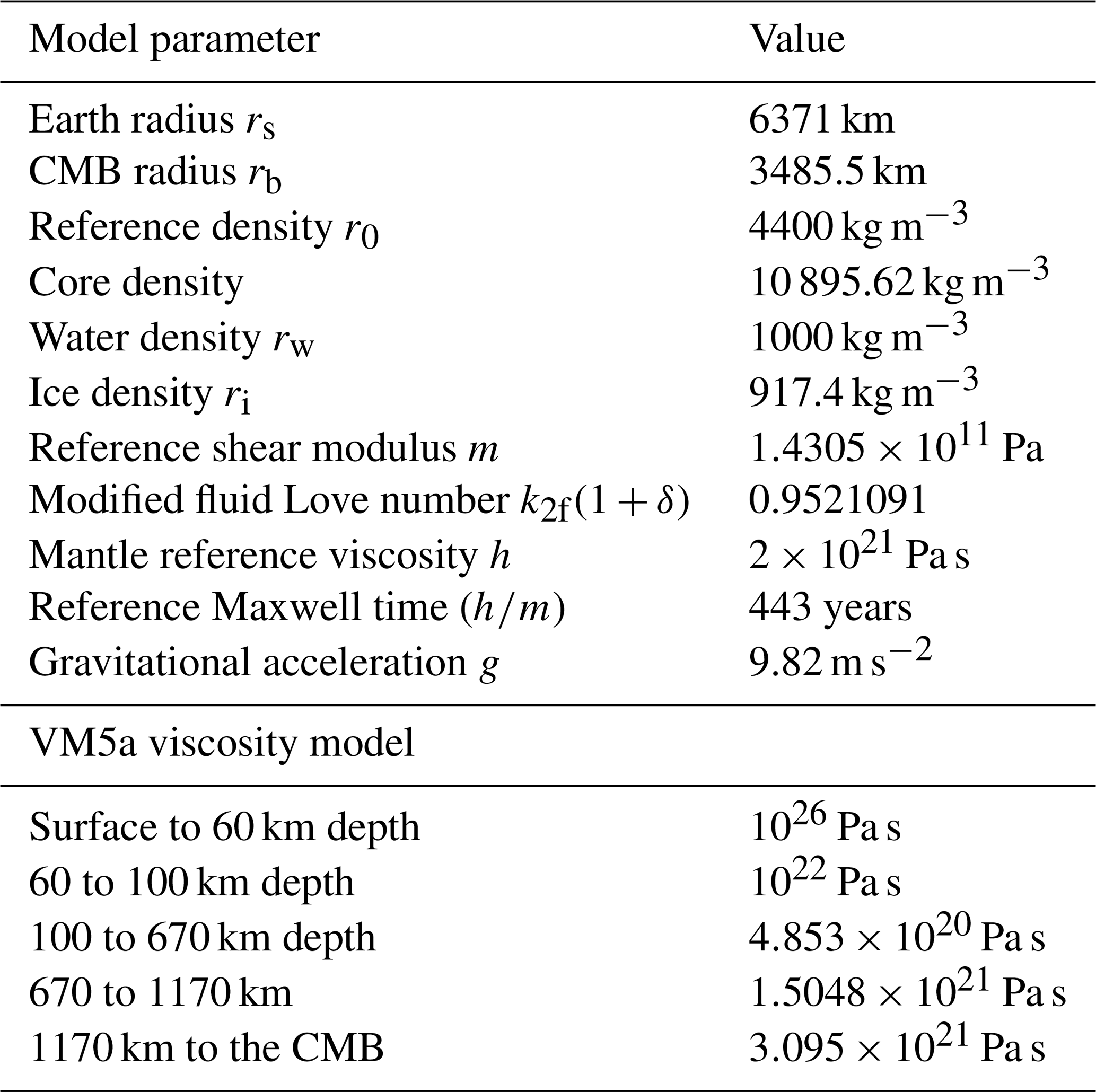
Table 2 Comparison of load Love numbers h_l, k_l, and l_l between CitcomSVE and semi-analytical solutions.

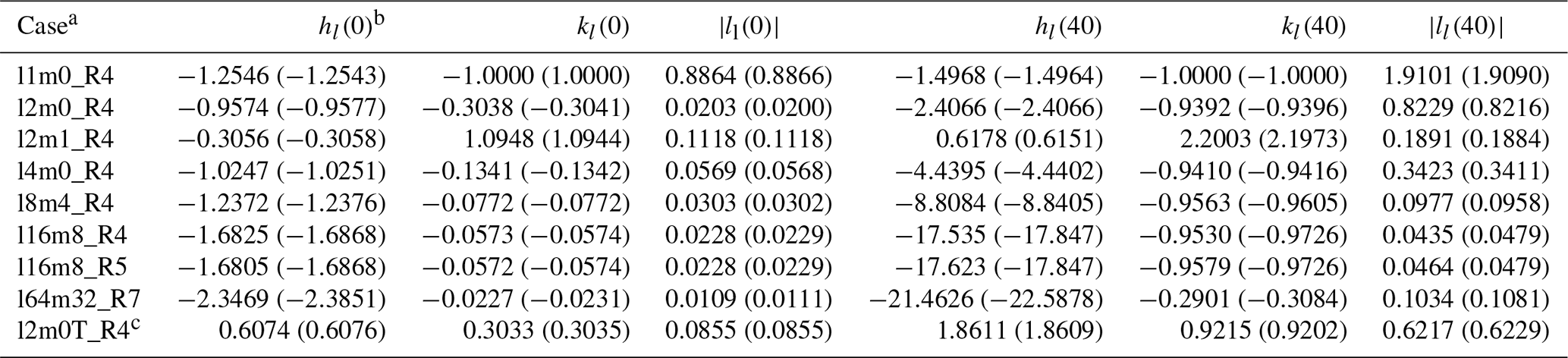
^a Case names follow this notation: l1m0 stands for the loading harmonics for l=1 and m=0. All CitcomSVE solutions in this table are for resolution R4 ($\mathrm{12}\times \mathrm{64}\times \mathrm{128}\times \mathrm{128}$), except for l16m8_R5 with a resolution of $\mathrm{12}\times \mathrm{80}\times \mathrm{128}\times \mathrm{128}$ (R5) and l64m32_R7 with a resolution of $\mathrm{12}\times \mathrm{80}\times \mathrm{256}\times \mathrm{256}$ (R7). ^b Load Love numbers are provided at 0 and 40 Maxwell times. Each entry includes semi-analytical solutions inside parentheses and CitcomSVE solutions outside parentheses. ^c l2m0T: tidal Love numbers for a Heaviside (2, 0) tidal load. Each entry includes semi-analytical solutions inside parentheses and CitcomSVE solutions (with a resolution of $\mathrm{12}\times \mathrm{64}\times \mathrm{128}\times \mathrm{128}$) outside parentheses.

3.1.2 Benchmark results

We have computed a set of model cases using CitcomSVE for four numerical resolutions and six loading harmonics. Seven different loading harmonics are included for (1, 0), (2, 0), (2, 1), (4, 0), (8, 4), (16, 8), and (64, 32), where the first and second numbers in parentheses (l, m) indicate the spherical harmonic degree l and order m, respectively. For the loading at the (2, 1) harmonic, the polar wander effect is considered. For most cases, the four different numerical resolutions of R1–R4 are for $\mathrm{12}\times (\mathrm{32}\times \mathrm{32}\times \mathrm{32})$, $\mathrm{12}\times (\mathrm{64}\times \mathrm{64}\times \mathrm{64})$, $\mathrm{12}\times (\mathrm{64}\times \mathrm{96}\times \mathrm{96})$, and $\mathrm{12}\times (\mathrm{64}\times \mathrm{128}\times \mathrm{128})$, respectively, where the first number, 12, indicates the number of spherical caps that the spherical surface is divided into and the subsequent numbers indicate the number of elements in the radial direction and two horizontal directions in each cap (Zhong et al., 2022). Each case is named according to its loading harmonic and numerical resolution; for example, case l2m0_R1 corresponds to the case where the loading harmonic is (2, 0) and the resolution is R1. For case l16m8, an additional calculation with resolution $\mathrm{12}\times (\mathrm{80}\times \mathrm{128}\times \mathrm{128})$ is included (i.e., l16m8_R5). For case l64m32, which has a much shorter loading wavelength and requires higher numerical resolutions, four calculations with resolutions of R5–R8 are included (Fig. 1), where R6–R8 are $\mathrm{12}\times (\mathrm{80}\times \mathrm{192}\times \mathrm{192})$, $\mathrm{12}\times (\mathrm{80}\times \mathrm{256}\times \mathrm{256})$, and $\mathrm{12}\times (\mathrm{96}\times \mathrm{256}\times \mathrm{256})$, respectively. Grid size in the vertical direction is not uniform since grids are refined vertically in the upper mantle and lithosphere for each model. For cases with 64 elements in the vertical direction (R2, R3, and R4), the vertical resolutions are about 20 km, 40 km, and more than 50 km in the lithosphere, upper mantle, and lower mantle, respectively. R5, with a total of 80 elements in the vertical direction, has vertical resolutions of ∼10 km in the lithosphere and ∼20 km in the upper mantle, whereas R8 is ∼7 km in the lithosphere and ∼10 km in the upper mantle. Each case is computed for 40 Maxwell times (i.e., 40a or a non-dimensional time of 40) using a non-dimensional time increment of 0.2. Figure 1 shows h_l(t), k_l(t), and |l_l(t)| for cases with different loading harmonics and numerical resolutions, together with semi-analytical solutions. Table 2 shows both numerical and analytical results of these Love numbers at t=0 and 40 for a selected set of cases (see Table S1 in the Supplement for all the cases). Solutions at t=0 represent the elastic responses of Earth, and the magnitudes of those Love numbers generally increase with time due to viscous relaxation and finally reach nearly stable states after certain time periods (Fig. 1).

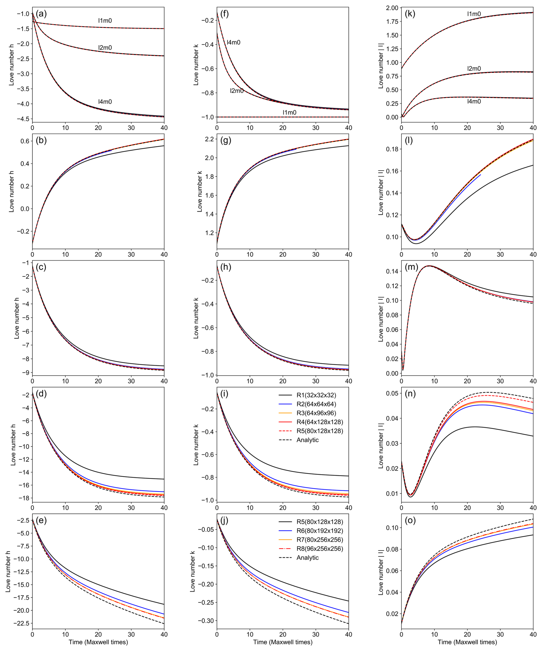
Figure 1 Love numbers h, k, and l for cases with different loading harmonics from CitcomSVE and analytical solutions. The first, second, and third columns are for Love numbers h, k, and |l| (i.e., the absolute values of Love number l), respectively. The first row (a, f, k) is for loading harmonics l1m0, l2m0, and l4m0. The following rows (b–o) are for loading harmonics l2m1, l8m4, l16m8, and l64m32, respectively. Each loading case has solutions from four different spatial resolutions (R1–R4), except that loading case l16m8 has an additional calculation with resolution R5, and cases with l64m32 (i.e., e, j, o) have resolutions from R5 to R8. Note that the legend in panel (i) is used for all the panels, except those in the last row (e, j, o).

The comparison shows good agreement between numerical solutions and semi-analytical solutions. For long-wavelength loadings (e.g., l1m0, l2m0, l2m0T, and l4m0), numerical solutions at different resolutions (R1–R4) are nearly identical to semi-analytical solutions, as shown in Fig. 1. However, for l2m1 cases with the polar wander effect, resolution R1 shows significant numerical errors, whereas calculations with higher resolutions (R2–R4) deliver a remarkable fit to the semi-analytical solution, suggesting that polar wander is more challenging to compute in numerical models (e.g., Paulson et al., 2005; A et al., 2013; Zhong et al., 2022). For shorter wavelengths (such as l8m4, l16m8, and l64m32), low-resolution numerical results differ noticeably from semi-analytical solutions. As the numerical resolution increases, the results match the semi-analytical solutions much more closely (Fig. 1). For case l16m8, R5 significantly reduces errors in l_l compared to R4. Note that R5 has a higher vertical resolution in the upper mantle but the same horizontal resolution as R4 (Fig. 1 and Table 2). For case l64m32, increasing vertical resolution does not reduce the misfit from R7 to R8, indicating that horizontal resolution is the controlling factor. Note that the load Love number for horizontal displacement is presented as $\left|l_l\right(t\left)\right|$, because CitcomSVE only conveniently determines $l_l^{\mathrm{2}}\left(t\right)$ (Zhong et al., 2022), although it is possible to determine l_l based on vector spherical harmonic decomposition of horizontal surface motion (Wu and Peltier, 1982).

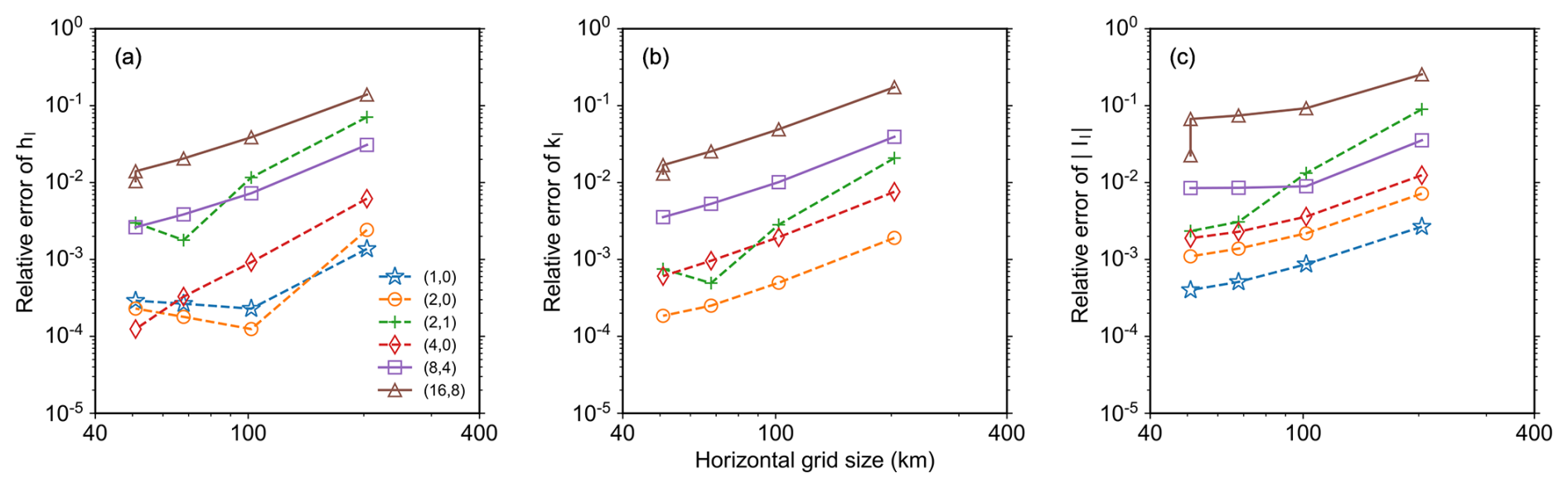
Figure 2 Amplitude errors of Love numbers h (a), k (b), and l (c) as functions of numerical resolutions (i.e., R1–R4, corresponding to horizontal resolutions of approximately 200 to 50 km). For Love number k of load (1, 0), all calculations with different resolutions have a relative error of less than 10⁻⁵ and are not shown in this figure. Note that R4 and R5 have the same horizontal resolution but different vertical resolutions, and R5 has smaller relative errors compared to R4.

We determine the numerical errors by computing amplitude and dispersion errors (e.g., Zhong et al., 2003, 2022; A et al., 2013). Amplitude error ε_a and dispersion error ε_d are computed using the following equations (Zhong et al., 2022):

$$\begin{array}{}\text{(14)}& {\displaystyle }& {\displaystyle }{\mathit{\epsilon }}_{\mathrm{a}}={\displaystyle \frac{\underset{\mathrm{0}}{\overset{T}{\int }}\mathrm{|}{S}_{\mathrm{n}}\left(l_{\mathrm{0}},m_{\mathrm{0}},t\right)-S_{\mathrm{sa}}\left(l_{\mathrm{0}},m_{\mathrm{0}},t\right)\mathrm{|}\mathrm{d}t}{\underset{\mathrm{0}}{\overset{T}{\int }}\mathrm{|}{S}_{\mathrm{sa}}\left(l_{\mathrm{0}},m_{\mathrm{0}},t\right)\mathrm{|}\mathrm{d}t}},\text{(15)}& {\displaystyle }& {\displaystyle }{\mathit{\epsilon }}_{\mathrm{d}}={\displaystyle \frac{\underset{\mathrm{0}}{\overset{T}{\int }}\max \left[\left|S_{\mathrm{n}}(l,m,t)\right|\right]\mathrm{d}t}{\underset{\mathrm{0}}{\overset{T}{\int }}\mathrm{|}{S}_{\mathrm{sa}}\left(l_{\mathrm{0}},m_{\mathrm{0}},t\right)\mathrm{|}\mathrm{d}t}},\end{array}$$

where l₀ and m₀ represent the loading harmonic degree and order, S_n and S_sa are solutions of load Love numbers from the CitcomSVE and semi-analytical methods, T is the total model time (i.e., 40), and in Eq. (15) for the dispersion error max represents the maximum value for all the non-loading harmonic degrees l and orders m. The response should only occur at the loading harmonic for the spherically symmetric mantle structure considered here. Therefore, amplitude error ε_a measures the accuracy at the loading harmonic and dispersion error ε_d measures the accuracy at other harmonics. Note that the errors defined in Eqs. (14) and (15) are similar to norm-1 errors.

Figure 2 shows the amplitude errors of load Love numbers as a function of horizontal numerical resolution (i.e., the horizontal grid size ranging from ∼200 to ∼50 at the surface for resolutions R1–R4) for all the cases except l64m32, which has a different range of horizontal resolutions. For most of the calculations with different loading harmonics, the amplitude errors decrease with decreasing horizontal grid size with a slope of close to 2 in the log–log plot of Fig. 2, especially for Love numbers h_l and k_l. This suggests that the error is roughly proportional to the square of the grid size, aligning with the expected second-order accuracy for trilinear elements in CitcomS (e.g., Zhong et al., 2008). It is worth noting that, from R1 to R4, the increase in vertical resolution is not proportional to the increase in horizontal resolution, which may cause the slope in Fig. 2 to deviate from 2. Figure 2 shows that, with a horizontal resolution of ∼50 km, the accuracy of CitcomSVE is better than 0.1 % up to spherical harmonics of degree 4 and better than 2 % up to spherical harmonics of degree 16 in terms of Love numbers h_l and k_l. For Love number l_l, the errors are slightly larger than those for h_l and k_l. Compared to the benchmark results of CitcomSVE-2.1 (Zhong et al., 2022), the errors presented here are generally larger for cases with the same resolutions, which is understandable considering that CitcomSVE-3.0 solves for models with higher complexity (i.e., the internal density variations caused by compressibility and density discontinuities).

3.2 Glacial isostatic adjustment using ICE-6G_D and VM5a

Since one of the most important applications of CitcomSVE is to model the GIA processes, it is essential to perform a benchmark with the glaciation–deglaciation history as surface loads, considering the effects of polar wander, apparent center of mass motion, and ocean loads determined by the sea level equation. A GIA model calculation requires the governing equations (Eqs. 1–3) to be solved together with the boundary conditions (Eqs. 4 and 5) and the sea level equation (Eq. 11), with the floating ice criterion to determine time-dependent gravitational potential anomalies and displacements at Earth's surface and sea level changes. Note that the same type of benchmark has been published for the incompressible version CitcomSVE-2.1 (Zhong et al., 2022), and we largely follow the setups of that previous work, except that the current calculations consider mantle compressibility (i.e., the PREM model) and the updated sea level equation is used as discussed above and in the Supplement (i.e., the AS1 method). As discussed in Sect. 2.3, to deal with the nonlinear nature of the sea level equation, multiple (usually three to four) iterations of complete GIA model runs may be needed (Kendall et al., 2005). CitcomSVE-3.0 fully supports the multiple-outer-iteration approach using preprocessing and postprocessing to update ocean functions and the initial topography. However, in the Supplement (Supplementary Text 2), we demonstrate how the one-iteration solution method discussed in Sect. 2.3 may be used to achieve adequate accuracy of GIA solutions. In the following GIA benchmark, we compare the results from a single complete CitcomSVE model run with our semi-analytical solutions of the first outer iteration (i.e., the AS1 method in the Supplement), using the precalculated ocean functions constructed by assuming a “rigid Earth” and the present-day topography as the initial topography. This comparison ensures that CitcomSVE and semi-analytical calculations have the same ocean functions and initial topography, such that the differences in solutions between the CitcomSVE and semi-analytical methods are solely related to numerical errors and not differences in the models.

3.2.1 Definition of the GIA problem

This section presents the setup of the GIA benchmark with the ICE-6G_D ice model (Peltier et al., 2015). The Earth model used in this case is the same as the one used for single harmonic loading examples in the previous section. In this case, the surface load consists of a full glaciation–deglaciation cycle based on the ICE-6G_D ice model (Peltier et al., 2015, 2018) that includes the last 122 kyr from the last interglacial period to the present day. We assume that Earth was in a state of equilibrium at the onset of loading (i.e., 122 ka BP) and that the surface displacements and gravitational potential anomalies since 122 ka BP have been induced by ice height variations relative to the initial stage and the corresponding changes in ocean loads. We computed seven cases using CitcomSVE-3.0 with different spatiotemporal resolutions and cutoff values for the maximum spherical harmonic degrees used to calculate the gravitational potential (Table 3). Cases GIA_R1, GIA_R2, and GIA_R3 have spatial resolutions of 135, 81, and 50 km (i.e., total element numbers of $\mathrm{12}\times \mathrm{48}\times \mathrm{48}\times \mathrm{48}$, $\mathrm{12}\times \mathrm{48}\times \mathrm{80}\times \mathrm{80}$, and $\mathrm{12}\times \mathrm{64}\times \mathrm{128}\times \mathrm{128}$), respectively, and a temporal resolution of 125 years per step. Case GIA_R3_LT is the same as case GIA_R3, except with a longer time increment of 250 years per step before the LGM (i.e., 26 ka BP). Cases GIA_R3_LT_SH20 and GIA_R3_LT_SH64 have cutoff values of 20 and 64 for the maximum spherical harmonic degrees compared to 32 for the other cases. Note that, as with CitcomSVE-2.1 (Zhong et al., 2022), computing gravitational potential in the spherical harmonic domain can be computationally expensive. On the other hand, the semi-analytical solution is obtained using spherical harmonic degrees and orders up to 256.

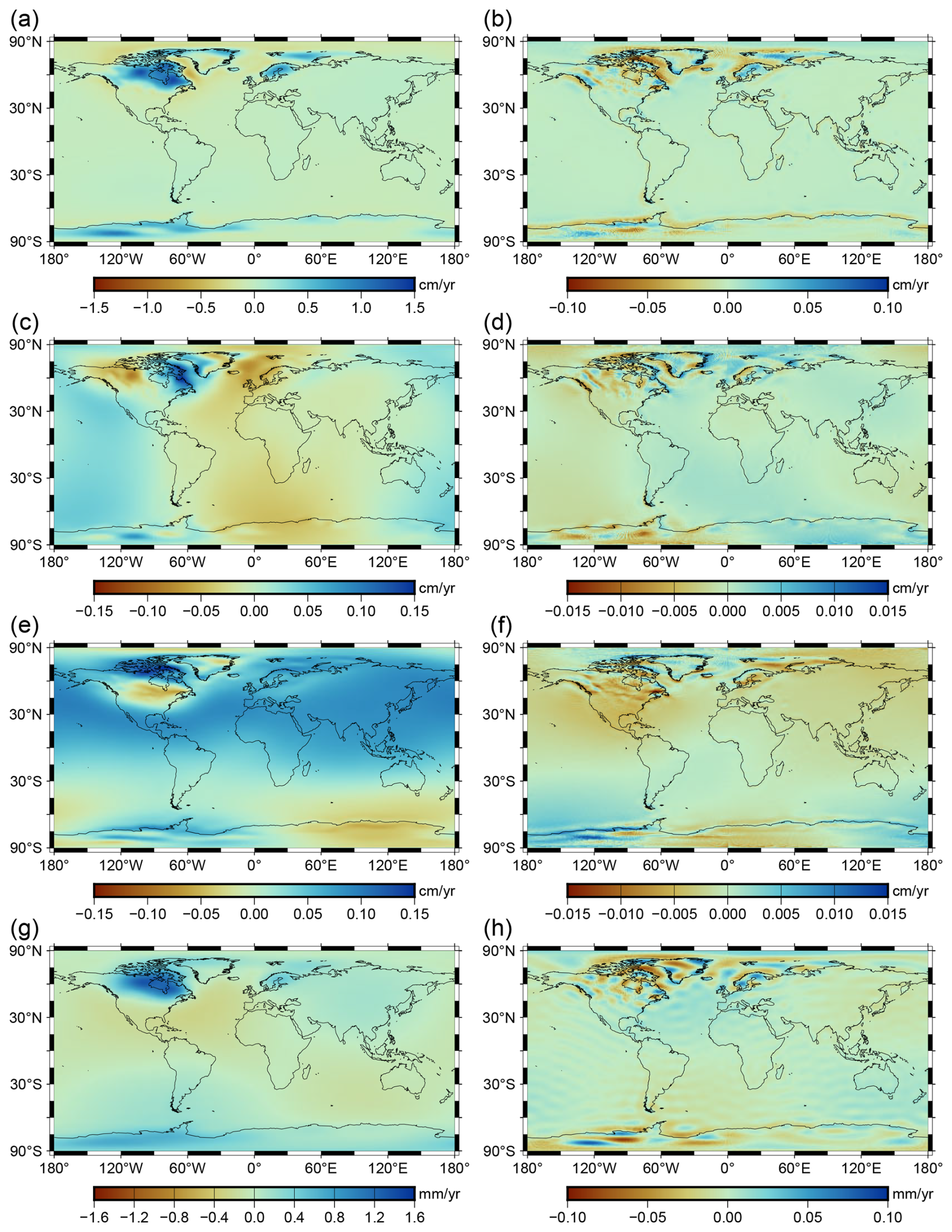
Figure 3 Displacement rate and geoid rate for the present day from case GIA_R3 and their differences from semi-analytical solutions. The top three rows (a–f) show displacement rates in the radial (a), eastern (c), and northern (e) directions and the differences from semi-analytical solutions for the radial (b), eastern (d), and northern (f) directions. The last row (g, h) shows the geoid rate (g) and its differences from the semi-analytical solution (h).

Table 3 Relative errors for surface three-component displacement rates for the GIA benchmark.

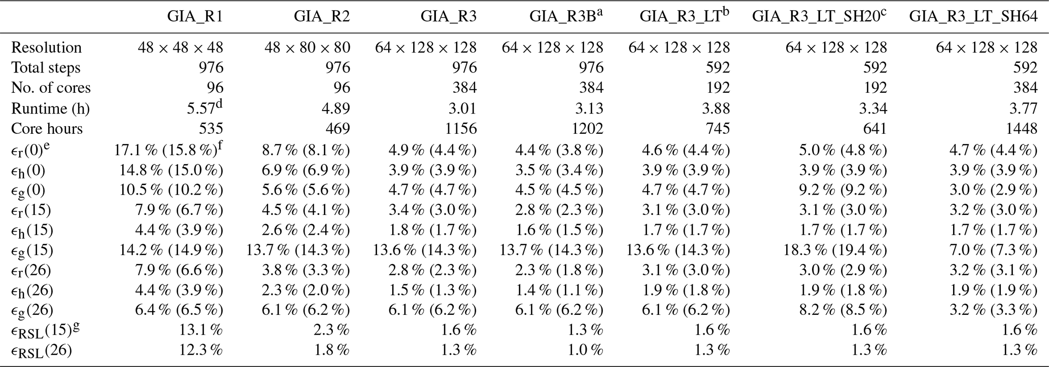
^a The differences between cases GIA_R3B and GIA_R3 are discussed in Sect. 3.2.1. ^b The “LT” in GIA_R3_LT means larger time increments between time steps, where the increments are 250 and 125 years before and after 26 ka BP, respectively. Cases GIA_R1, GIA_R2, and GIA_R3 have a uniform time increment of 125 years. ^c The “SH20” in GIA_R3_LT_SH20 means that the cutoff of degrees and orders of spherical harmonics in this calculation is 20. Similarly, case GIA_R3_LT_SH64 has a cutoff at degrees and orders of 64. Other cases are cut off at degrees and orders of 32. ^d For this case, the solution converges slowly, causing longer CPU times. All the cases are computed on the NCAR supercomputer Derecho. ^e ϵ_r, ϵ_h, and ϵ_g are errors of displacement rates in the radial and horizontal directions and errors of geoid rates, respectively. The errors are given for the present-day (0), 15 ka BP, and 26 ka BP. Note that the geoid rates include the contribution from the centrifugal potential. ^f Numbers outside parentheses are errors calculated based on regular grids, whereas numbers inside parentheses are calculated based on CitcomSVE grids. ^g ϵ_RSL is similar to ϵ_h but for relative sea level. The errors are calculated based on regular grids.

It should be noted that, in the current implementation, CitcomSVE reads in ice loads defined on regular grids (e.g., a 1°×1° grid) and then interpolates the loads to the irregular finite-element grids, whereas semi-analytical calculations use spherical harmonic expansions of ice loads to a maximum spherical harmonic degree and order (i.e., 256 in this study) as inputs. The interpolation may cause inconsistent representations of ice loads between CitcomSVE and the semi-analytical calculations. To understand the potential error resulting from the interpolation, we test another case, GIA_R3B, which is the same as GIA_R3, except that, for this case, we let CitcomSVE read in ice loads that are computed on CitcomSVE finite-element grid points by summing all the spherical harmonics as used for the analytical solutions, thus avoiding the interpolation from the regular grids to the finite-element grids and ensuring that CitcomSVE calculations use the exact same ice loads as for the analytical solutions.

3.2.2 Benchmark results

We compare the three-component displacement rates and geoid rates at the surface for three different times (i.e., the present day, 15 ka BP, and 26 ka BP) obtained from CitcomSVE and the semi-analytical code. Figure 3 shows the present-day displacement rate in the vertical, eastern, and northern directions and the present-day geoid rate for case GIA_R3 from CitcomSVE. Large uplift rates for the present day occur in North America, Fennoscandia, and West Antarctica (Fig. 3a), suggesting ongoing rebound induced by ice melting since the Last Glacial Maximum in these regions. Horizontal displacement rates usually have much smaller amplitudes than those in the radial direction in these regions.

Figure 3 also shows the differences in present-day displacement rates and geoid rates between CitcomSVE and semi-analytical solutions. The differences are small compared with the magnitudes of displacement rates and geoid rates. Relatively large magnitudes of errors are mainly in short wavelengths (e.g., localized regions), which may partially reflect the fact that CitcomSVE tends to have poorer accuracy at shorter wavelengths (Figs. 1 and 2). Following Zhong et al. (2022), we define relative root mean square (rms) differences (i.e., errors) in displacement rates between CitcomSVE and semi-analytical solutions as

$$\begin{array}{}\text{(16)}& \mathit{\epsilon }\left(t\right)=\sqrt{{\displaystyle \frac{\mathrm{\Sigma }{\left[f_{\mathrm{FE}}(\mathit{\theta },\mathit{\varphi },t)-f_{\mathrm{S}}(\mathit{\theta },\mathit{\varphi },t)\right]}^{\mathrm{2}}}{\mathrm{\Sigma }{\left[f_{\mathrm{S}}(\mathit{\theta },\mathit{\varphi },t)\right]}^{\mathrm{2}}}}},\end{array}$$

where $f_{\mathrm{FE}}(\mathit{\theta },\mathit{\varphi },t)$ and $f_{\mathrm{S}}(\mathit{\theta },\mathit{\varphi },t)$ are the fields of interest at a given time t from CitcomSVE and semi-analytical solutions, respectively, and the summation is based on a regular 1^°×1° grid. To interpolate the CitcomSVE solutions onto the regular grid, we use the nearest-neighbor method provided by generic mapping tools (GMTs) (Wessel et al., 2019). We also report errors calculated by unweighted summation on the CitcomSVE grid given the relatively uniform grid size on the spherical surface in CitcomSVE, and the differences in errors from these two methods of calculation are insignificant. We compute errors for radial and horizontal components at three times: the present day, 15 ka BP, and 26 ka BP. Note that, for horizontal error, we square the difference for each horizontal component (i.e., north and east) and add them together for each location.

Table 3 lists the errors for displacement rates, geoid rates, and RSL at these three times for all the cases, together with the total CPU time and the number of CPUs used for each case. The errors decrease significantly from GIA_R1 to GIA_R3. For GIA_R3, the errors of displacement rates are less than 5 %. GIA_R3B, which avoids interpolation of input ice loads from the regular input grid into the CitcomSVE finite-element grid in order to eliminate the potential inconsistency in ice loads between CitcomSVE and semi-analytical calculations, has slightly smaller errors than GIA_R3, indicating a relatively small error induced by the interpolation. GIA_R3_LT with a higher time resolution before 26 ka BP has larger errors in displacement rates at 26 ka BP but similar error levels at 15 ka BP and the present day. For geoid rates, since CitcomSVE-3.0 only calculates them up to certain degrees (i.e., degrees 20, 32, or 64 in our cases), which are much smaller than that used in the analytical solution (i.e., degree 256), the solutions from CitcomSVE-3.0 lack short-wavelength features and are much smoother spatially, even for cases with high grid resolutions. Therefore, the errors in geoid rates are larger and generally less sensitive to model resolutions than to cutoff degrees. In general, those errors in displacement rates are close to those from CitcomSVE-2.1 (Zhong et al., 2022). CitcomSVE-3.0 is about 3 times slower than CitcomSVE-2.1 for the same resolutions since internal density variations make the computation more expensive, as discussed in Sect. 2.2. We found that, for GIA_R1, GIA_R2, and GIA_R3, calculating gravitational potential anomalies takes up about one-fourth to half of the total calculation times, depending on the time spent solving the displacement field. It is possible to speed up the calculations of the gravitational potential anomalies by using a grid-based method (e.g., Latychev et al., 2005) or direct integration (e.g., Wang and Li, 2021) for the Poisson equation instead of the currently used spherical harmonic transform. The maximum degree of spherical harmonics used for potential calculation, varying between 20 (GIA_R3_LT_SH20), 32 (GIA_R3_LT), and 64 (GIA_R3_LT_SH64), affects the modeled change rates of geoid and gravity, as shown in the varying errors of the geoid rates (Table 3), such that the error decreases with an increasing maximum degree. However, it has insignificant effects on surface displacement and RSL (Tables 3 and 4).

Table 4 Relative errors for surface radial displacements at different harmonics.

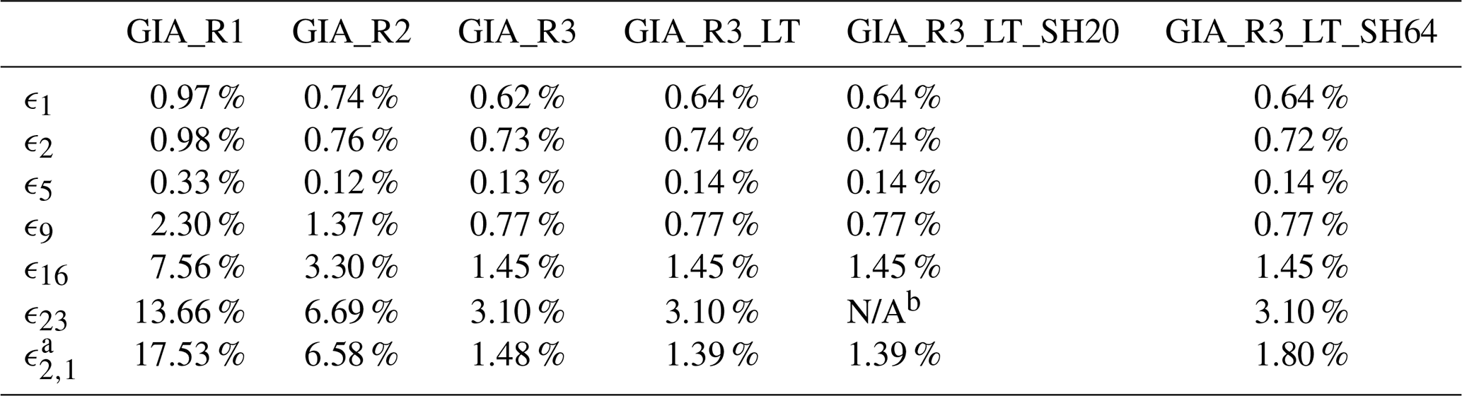
^a ϵ_2,1 represents the errors for the polar wander term (l=2, m=1). ^b N/A, the cutoff of degrees and orders of spherical harmonics, is 20 for this case, and we only output the spherical harmonics up to the cutoff value in CitcomSVE.

We also compare the cumulative radial displacements at different spherical harmonic degrees from the CitcomSVE and semi-analytical solutions, following previous works (Paulson et al., 2005; A et al., 2013; Kang et al., 2022; Zhong et al., 2022). The spherical harmonic coefficients of the surface displacement field are provided as an output of CitcomSVE (see Zhong et al., 2022, for the spherical harmonic expansion used in CitcomSVE). The degree amplitude for each l is calculated by

$$\begin{array}{}\text{(17)}& a_l\left(t\right)=\sqrt{{\displaystyle \frac{\mathrm{1}}{l+\mathrm{1}}}\sum _{m=\mathrm{0}}^l\left[C_{lm}(t{)}^{\mathrm{2}}+S_{lm}(t{)}^{\mathrm{2}}\right]},\end{array}$$

where C_lm and S_lm denote the cosine and sine parts of the spherical harmonic coefficients expanded from the radial displacement fields at time t. Figure 4a–c show the amplitude a_l of surface radial displacement at selected spherical harmonic degrees (l=1, 2, 5, 9, 16, and 23) for the three CitcomSVE cases, together with the corresponding semi-analytical solutions. As with CitcomSVE-2.1 (Zhong et al., 2022), the lowest-resolution case is adequate for relatively long wavelengths (l=1, 2, 5, and 9), whereas higher-resolution models are required for accuracy at shorter wavelengths (l=16 and 23) (Fig. 4c). Figure 4d shows the results for the harmonic of l=2 and m=1 that corresponds to the polar wander. Similar to findings from single harmonic benchmarks in the previous section and Zhong et al. (2022), high spatial resolution is required to obtain an accurate solution for the polar wander term. Note that the amplitudes of the polar wander mode are much smaller than other long-wavelength modes like l=2, 5, and 9.

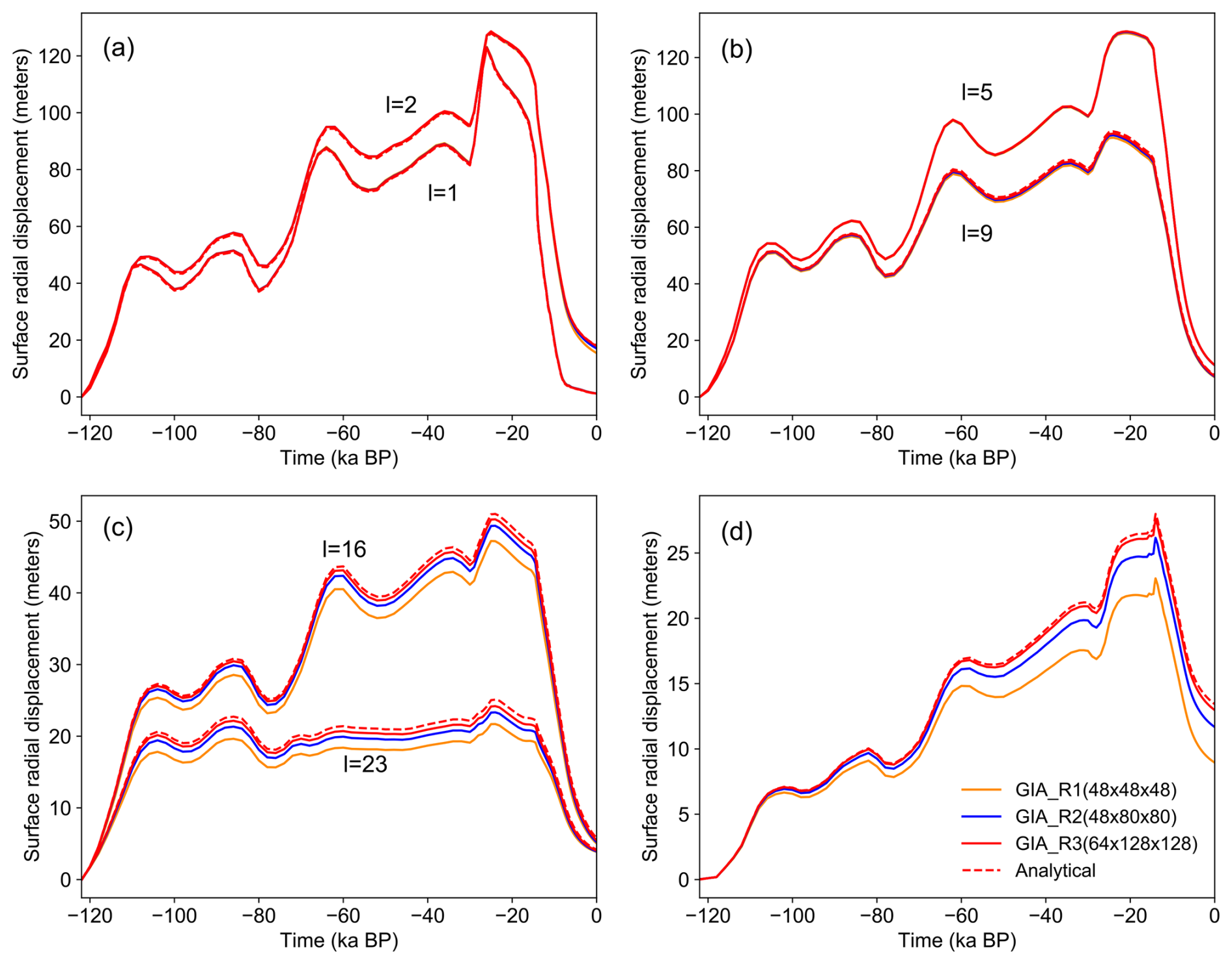
Figure 4 Amplitudes of cumulative radial surface displacement at different spherical harmonic degrees as a function of time for the semi-analytical solutions (Analytical) and three CitcomSVE calculations (GIA_R1, GIA_R2, and GIA_R3) for $l=\mathrm{1},\mathrm{2}$ (a), $l=\mathrm{5},\mathrm{9}$ (b), $l=\mathrm{16},\mathrm{23}$ (c), and the polar wander mode with l=2, m=1 (d).

Following Zhong et al. (2022), we use the time-integrated relative error of degree amplitude ε_l to quantify the time-averaged error for a given degree l. ε_l is defined as

$$\begin{array}{}\text{(18)}& {\mathit{ϵ}}_l=\sqrt{{\displaystyle \frac{\underset{\mathrm{0}}{\overset{T}{\int }}{\left[a_{l_{\mathrm{FE}}}\left(t\right)-a_{l_{\mathrm{S}}}\left(t\right)\right]}^{\mathrm{2}}\mathrm{d}t}{\underset{\mathrm{0}}{\overset{T}{\int }}{a}_{l_{\mathrm{S}}}(t{)}^{\mathrm{2}}\mathrm{d}t}}},\end{array}$$

where $a_{l_{\mathrm{FE}}}\left(t\right)$ and $a_{l_{\mathrm{S}}}\left(t\right)$ represent the degree amplitudes at time t from the CitcomSVE and semi-analytical solutions, respectively, and T is the entire calculation period. The errors for each case are shown in Table 4. As expected, the errors decrease with increasing spatial resolution for each degree, and errors for shorter wavelengths are larger than those for longer wavelengths, except for the polar wander term with relatively large errors.

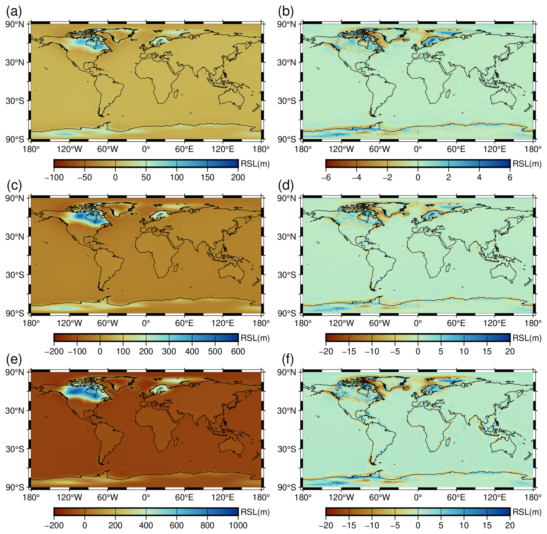
Figure 5 Map of the modeled relative sea levels at 5 ka BP (a), 10 ka BP (c), and 15 ka BP (e) from GIA_R3 and their differences from semi-analytical solutions at 5 ka BP (b), 10 ka BP (d), and 15 ka BP (f), respectively.

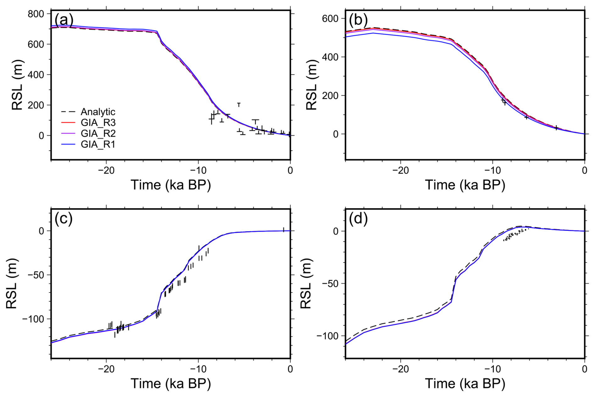
Figure 6 Relative sea level curves for the last 26 kyr at four sites from semi-analytical solutions (Analytic) and three CitcomSVE calculations at different resolutions: cases GIA_R1, GIA_R2, and GIA_R3. The four sites are Churchill (a), Vasterbotten (b), Barbados (c), and Geylang (d) with latitudes and longitudes of (58.70, 265.60), (64.00, 19.90), (13.04, 300.45), and (1.31, 103.87), respectively. The symbols represent the observed RSL changes. The observed RSL values are from Peltier et al. (2015) and Lambeck et al. (2014).

Figure 5 shows the comparisons of modeled relative sea levels at different periods (5, 10, and 15 ka BP) for GIA_R3 and the semi-analytical solutions on map views. The regions with localized, relatively large errors (Fig. 5b, d, and f) are mostly around the edges of ice sheets in North America, Fennoscandia, and Antarctica, similar to those for the displacement rates as shown in Fig. 3b. Figure 6 compares modeled RSL curves for several sites from semi-analytical solutions and three CitcomSVE calculations with different spatial resolutions. Increasing spatial resolution reduces the offsets to semi-analytical solutions for near-field sites (i.e., sites close to ice sheets) (Fig. 6a and b) but does not appear to affect the far-field solutions as much (Fig. 6c and d), reflecting the facts that the RSL at far-field sites is not sensitive to numerical resolutions and the offsets to semi-analytical solutions are caused by other factors, e.g., the interpolation of the ocean function from a regular grid to the CitcomSVE grid or the interpolation of results on the CitcomSVE grid to RSL sites.

4 Conclusion and discussion

This study introduces CitcomSVE-3.0, an enhanced finite-element package that builds upon its predecessor CitcomSVE-2.1 (Zhong et al., 2022), an efficient package that utilizes massively parallelized computers with up to thousands of CPUs. The new version incorporates elastic compressibility (e.g., the PREM model) based on the work of A et al. (2013) and improves the algorithm for solving sea level equations following the work of Kendall et al. (2005), which considers the changes in ocean loads and ocean functions related to ocean–continent transitions and the existence of floating ice. Two benchmark problems are computed with different numerical resolutions: (1) surface and tidal loads of different single harmonics and (2) the GIA problem with the ICE6G_D ice model.

Extensive comparisons between CitcomSVE-3.0 calculations and semi-analytical solutions are presented to validate the accuracy of the CitcomSVE package. The accuracy of CitcomSVE with a horizontal resolution of ∼50 km is better than 0.1 % up to spherical harmonics of degree 4 and better than 2 % up to degree 16 in vertical motion and gravitational potential for single harmonic loading problems. The single harmonic benchmarks show that CitcomSVE has a second order of accuracy; i.e., the errors would be reduced to 0.25 if the element sizes were reduced by a factor of 2. For GIA problems with realistic ice models and dynamically determined ocean loads, the average errors for CitcomSVE models with ∼50 km horizontal resolution are less than 5 % in displacement rates and relative sea levels.

As shown in the benchmark work for CitcomSVE-2.1 (Zhong et al., 2022), CitcomSVE has a parallel computational efficiency of >75 % for up to 6144 CPU cores. Although CitcomSVE-3.0 is about 3 times slower than CitcomSVE-2.1 for most of our tests because of the added computational expense for gravitational potential introduced by the layered density structure and compressibility, it can complete a high-resolution global GIA calculation within several hours on supercomputers with a modest number of CPU cores. With its accuracy and efficiency in modeling viscoelastic responses to surface loads and tidal forces, the open-source package CitcomSVE has the ability to advance research in planetary and climatic sciences, including GIA-related problems.