Improvement of near-surface wind speed modeling through refined aerodynamic roughness length in high-roughness surface regions: implementation and validation in the Weather Research and Forecasting (WRF) model version 4.0

Aerodynamic roughness length (z₀) is a key parameter determining near-surface wind profiles, significantly influencing wind-related studies and applications. In high-roughness surface areas, surface roughness has been substantially altered by land use changes such as urbanization. However, many numerical models still assign long-standing and fixed z₀ based on traditional land cover types, neither accounting for shifts in land cover nor updating class-specific z₀, leaving z₀ values in high-roughness surface regions outdated and unreliable. To address this issue, this study proposed a cost-effective method to estimate z₀ values at weather stations by adjusting z₀ values to minimize the wind speed differences between ERA5 reanalysis data and weather station observation data. Using this approach, z₀ values were derived for 1837 stations in the high-roughness surface areas across China. Based on these estimates, a high-resolution monthly gridded z₀ dataset was then developed for high-roughness surface areas in China using Random Forest Regression algorithm. Simulations with Weather Research and Forecasting (WRF) model show that implementation of the new z₀ dataset significantly improves the accuracy of 10 m wind speed over high-roughness surface areas, reducing mean wind speed errors by 79.8 % and 78.0 % compared to the default z₀ in WRF and a latest gridded z₀ dataset from Peng et al. (2022), respectively. Independent validations of 100 m wind speed against anemometer tower data further confirm the dataset's reliability. Therefore, this approach is valuable for wind-dependent studies and applications, such as urban planning, air quality management, and wind energy utilization, by enabling more accurate simulations of wind speed in high-roughness surface areas.

1 Introduction

With the rapid advancement of urbanization and industrialization, human activities and energy use are increasingly concentrated along the settlement-landscape continuum (Liu et al., 2014), particularly in high-roughness areas such as built-up zones and inhabited vegetated landscapes. High-roughness surface regions not only significantly influence climate change but also are highly sensitive to meteorological and climatic conditions (Kammen and Sunter, 2016). Among various meteorological parameters, wind speed exerts great impacts on both environmental and human systems. One prominent example is that wind speed is a crucial consideration for assessing the atmospheric pollutant dispersion capability (Manju et al., 2002; Han et al., 2017). Specifically, mean flows and atmospheric turbulence are two key factors for pollutant removal (Wong and Liu, 2013; Di Nicola et al., 2022). Also, wind speed regulates pollen dispersion and distribution that are associated with public health (Roy et al., 2023). The utilization of wind energy in high-roughness surface areas also depends on wind speed distribution (Ishugah et al., 2014; Stathopoulos et al., 2018; Tasneem et al., 2020). Proper utilization, through measures such as suburban wind farms or building-integrated turbines, can minimize the need for transmission infrastructure. Beyond energy considerations, wind speed characteristics play a critical role in design and planning of human settlements, influencing both contemporary building practices (Hadavi and Pasdarshahri, 2020) and the preservation of historical-cultural heritage (Li et al., 2021). Therefore, accurately characterizing wind speed is essential for guiding systematic regulation and promoting sustainable development in high-roughness surface areas.

Aerodynamic roughness length (z₀) is a crucial parameter that determines near-surface wind speed profiles (Stull, 1988). As a key input for atmospheric models, z₀ significantly influences wind speed-related applications, however, its representation in existing numerical models often oversimplifies real-world conditions. Specifically, most models, such as the widely used European Centre for Medium-Range Weather Forecasts Reanalysis v5 (ERA5), determine z₀ with long-standing and fixed values based on traditional land cover types. Such treatment fails to reflect the impact of transitions between surface types and changes in roughness elements within the same type, particularly the complexity of urban structures, thereby posing significant challenges for accurate wind speed simulation and prediction over high-roughness surface areas (Wang et al., 2024). Numerous studies have demonstrated that the changes of z₀, caused by land use changes, particularly urbanization and industrialization, as well as deforestation and afforestation, significantly impacted wind speed. For instance, the increase in z₀ has explained 70 % of the wind speed reduction in Europe (Wever, 2012) and caused a 1.1 m s⁻¹ decrease in eastern China (Wu et al., 2017). Furthermore, Zhang et al. (2019) identified z₀ changes as a primary driver of long-term wind speed trends in China, Europe, and North America. In line with these findings, Luu et al. (2023) showed that the rise in z₀, caused by shifts from short vegetation to high vegetation and urbanization, partly contributes to the decline in mean and maximum surface wind speed over Western Europe. A similar mechanism operated in Canada. At Sudbury Airport (Ontario), 10 m wind speeds declined by ∼34 % during 1975–1995 mainly due to reforestation-induced increases in surface roughness (Tanentzap et al., 2007). These findings highlight the need to refine z₀ in models by incorporating the effects of high-roughness surface areas across urban-town settings and tall-vegetation landscapes. In addition to wind speed, z₀ also plays a significant role in environmental processes. The difference in z₀ between urban and suburban areas is one of drivers causing larger intensity of daytime urban heat islands in humid regions (Zhao et al., 2014; Li et al., 2019). Winckler et al. (2019) showed that roughness changes are a primary control on deforestation's biogeophysical effects, notably surface temperature responses. Therefore, accurate z₀ data in high-roughness surface areas can not only enhance the performance of atmospheric numerical models, but also provide scientific support for formulating sustainable urban environmental management strategies.

The estimation of z₀ in high-roughness surface areas traditionally relies on three primary approaches: the micrometeorological method, the morphometric method, and a combination of these two methods. The micrometeorological method, based on the Monin-Obukhov similarity theory (Monin and Obukhov, 1954), typically calculates z₀ using observations from flux or anemometer towers (Grimmond et al., 1998; Liu et al., 2018). Although theoretically robust, this method is limited by high costs of instruments and infrastructure (Grimmond and Oke, 1999), as well as the need for homogeneous surface conditions (Wieringa, 1993; Bottema and Mestayer, 1998). The morphometric method usually formulates mathematical models based on geometric characteristics and distribution density of high-roughness surface areas (Raupach, 1992, 1994; Bottema and Mestayer, 1998; Macdonald et al., 1998; Kanda et al.,2013; Shen et al., 2022, 2024). However, these models often suffer from simplified assumptions and require high-resolution surface feature data, which are costly to acquire (Grimmond and Oke, 1999; Zhang et al., 2017). The combination method, which establishes a relationship between the z₀ ground truth obtained from micrometeorological method and high-resolution surface feature data for regional-scale applications, has shown promise in specific regions, such as Tokyo and Nagoya (Kanda et al., 2013), Beijing (Zhang et al., 2017), and Osaka subregions (Duan and Takemi, 2021). Nevertheless, the limitations of the former two methods hinder its broader applications. Therefore, there is a considerable lack of reliable z₀ data in high-roughness surface regions.

To address the aforementioned challenges, this study proposed a low-cost method for estimating z₀ by integrating 10 m wind speed at China Meteorological Administration (CMA) stations with 10 m wind speed and z₀ from ERA5 reanalysis data. This approach takes advantage of the synergy between CMA's high-density station distribution and ERA5 reanalysis' temporal continuity to substantially enhance the sample size of z₀ estimates. Based on these estimates, we have developed a high-resolution monthly z₀ dataset for high-roughness surface areas in China using Random Forest Regression (RFR) algorithm. The applicability of the new z₀ dataset has been assessed through its implementation in the Weather Research and Forecasting (WRF) model for wind speed simulation. This study contributes to the advancement of mesoscale wind speed simulation over high-roughness surface environments, which can promote wind field-dependent studies, such as urban planning, wind energy utilization, and air quality management.

2 Data and method

2.1 Data

In this study, we mainly utilized monthly gridded z₀ dataset from ERA5 (Hersbach et al., 2020, 2023a), referred to as z_{0_ERA5}, along with hourly 10 m wind speed data from both ERA5 (Hersbach et al., 2023b) and surface weather station observations provided by the(CMA) during 2015–2019, to derive z₀ estimates at each CMA station.

To extend the site-scale z₀ estimates into a gridded dataset at the regional scale, we applied the RFR algorithm, incorporating six key features: variance of the slope ($\stackrel{\mathrm{‾}}{{\mathit{\theta }}^{\mathrm{2}}}$), terrain standard deviation within 0.01° window (TSD), percent tree cover (PTC), leaf area index (LAI), normalized difference vegetation index (NDVI), and urban-rural classification (URC). $\stackrel{\mathrm{‾}}{{\mathit{\theta }}^{\mathrm{2}}}$ was derived as an integral over orographic spectrum, capturing multi-scale orographic complexity with wave length from meter to 10 km (Beljaars et al., 2004). We obtained $\stackrel{\mathrm{‾}}{{\mathit{\theta }}^{\mathrm{2}}}$ from the dataset accompanying the turbulent orographic form drag scheme in WRF (Zhou et al., 2018), which was processed from the global 30^′′ GMTED2010 digital elevation model (Danielson and Gesch, 2011). TSD was calculated using elevation data from Shuttle Radar Topography Mission with a spatial resolution of 3 arcsec (Jarvis et al., 2008). The PTC data were obtained from the MOD44B Version 6.1 Vegetation Continuous Fields product (DiMiceli et al., 2022), which provides yearly data at a 250 m pixel resolution. The monthly 1 km NDVI data were acquired from MOD13A3 product (Didan, 2021). The LAI data with an 8 d temporal interval and 500 m spatial resolution were sourced from Yuan et al. (2011) and Lin et al. (2023). URC data were extracted from a 1 km global human settlements map, which categorizes the rural-urban continuum into 19 distinct types (Li et al., 2022, 2023). To generate a monthly z₀ dataset at a spatial resolution of 0.01°×0.01°, all input datasets were linearly interpolated or resampled to the target resolution. LAI data were averaged monthly by assigning each 8-day interval to the closest month.

Additionally, to compare with the existed z₀ datasets, a latest z₀ dataset developed by Peng et al. (2022) (denoted as z_{0_Peng}) was used by integrating it into the WRF model for wind speed simulation. This dataset was generated by applying machine learning techniques to integrate FLUXNET ground-based observations and MODIS remote sensing data. Moreover, 100 m wind speed data from 589 anemometer towers in China were utilized for two critical purposes. First, the comparison between tower observations and ERA5 100 m wind speed data (Hersbach et al., 2023b) was used to validate the feasibility of the assumption in the z₀ estimation method. Second, tower data were used as independent validations to evaluate the impact of refined z₀ on wind speed simulations. These anemometer towers cover varying periods between 2004 and 2022 with a temporal resolution of 10 min.

2.2 Method for deriving z₀ at CMA stations

First, the theoretical basis for deriving z₀ at CMA stations is presented. In the framework of Monin-Obukhov similarity theory (Monin and Obukhov, 1954), the neutral logarithmic wind profile can be expressed with Eq. (1).

$$\begin{array}{}\text{(1)}& u_z={\displaystyle \frac{u_{*}}{k}}\ln \left({\displaystyle \frac{z-d}{z_{\mathrm{0}}}}\right)\end{array}$$

where u_z is the wind speed (m s⁻¹) at height z, the measuring height above ground (m); u_* is the friction velocity (m s⁻¹); k is the von Karman constant and equals to 0.4, and d is the zero-plane displacement height (m), calculated as $d=\mathrm{20}/\mathrm{3}{z}_{\mathrm{0}}$ using a widely accepted empirical formula (Watts et al., 2000).

Based on Eq. (1), the 100 m neutral wind speed for ERA5 and CMA stations can be expressed in Eqs. (2) and (3), respectively.

$$\begin{array}{}\text{(2)}& {\displaystyle }& {\displaystyle }{u}_{\mathrm{100}\mathrm{\_}\mathrm{ERA}\mathrm{5}}=u_{\mathrm{10}\mathrm{\_}\mathrm{ERA}\mathrm{5}}{\displaystyle \frac{\ln \left(\frac{\mathrm{100}-d_{\mathrm{ERA}\mathrm{5}}}{z_{\mathrm{0}\mathrm{\_}\mathrm{ERA}\mathrm{5}}}\right)}{\ln \left(\frac{\mathrm{10}-d_{\mathrm{ERA}\mathrm{5}}}{z_{\mathrm{0}\mathrm{\_}\mathrm{ERA}\mathrm{5}}}\right)}}\text{(3)}& {\displaystyle }& {\displaystyle }{u}_{\mathrm{100}\mathrm{\_}\mathrm{CMA}}=u_{\mathrm{10}\mathrm{\_}\mathrm{CMA}}{\displaystyle \frac{\ln \left(\frac{\mathrm{100}-d_{\mathrm{CMA}}}{z_{\mathrm{0}\mathrm{\_}\mathrm{CMA}}}\right)}{\ln \left(\frac{\mathrm{10}-d_{\mathrm{CMA}}}{z_{\mathrm{0}\mathrm{\_}\mathrm{CMA}}}\right)}}\end{array}$$

and then z₀ values at CMA stations can be estimated by the following three steps:

First, we assumed: (1) the near-surface wind speed difference between ERA5 and CMA is primarily attributed to z₀, and the influence of z₀ diminishes with height. Consequently, the 100 m wind speed from ERA5 reanalysis is considered comparable to that from observations; (2) the impact of atmospheric stability on wind speed is identical for both ERA5 and CMA stations, allowing us to neglect stability correction terms under non-neutral conditions when deriving z₀ for each hourly interval. The validity of these assumptions will be supported by the subsequent validation of wind speed simulations based on the derived z₀ values (Sect. 3.3).

Second, we calculated the hourly z_{0_CMA} values based on Eqs. (2) and (3). Given that u_{10_ERA5}, u_{10_CMA}, and z_{0_ERA5} values are known, an optimal z_{0_CMA} value at each hour was derived through minimizing the difference between u_{100_ERA5} and u_{100_CMA} calculated using Eqs. (2) and (3). To align with Assumption (1), we only retained z_{0_CMA} values corresponding to times when the percentage difference between the calculated u_{100_ERA5} and u_{100_CMA} was less than 10 %. ERA5 provides native 100 m winds, but here we use log-law – reconstructed 100 m winds from u_{10_ERA5} and z_{0_ERA5} instead. The reason is that the z_{0_CMA} is derived under the assumption that stability-correction term is neglected. This means that the 100 m wind speeds in Eqs. (2) and (3) are both calculated without considering stability effects. However, the native ERA5 100 m wind field inherently embeds model-diagnosed stability influences. Therefore, directly pairing native ERA5 100 m winds with our CMA log-law construction would amplify the error in the derived ln (z₀). In addition, the reconstruction offers two practical advantages. First, it requires fewer variables and a more transparent linkage, relying only on 10 m wind speeds and z₀ from reanalysis, together with 10 m wind speeds from observations; Second, our results indicate that the z₀ estimates are not particularly sensitive to the choice of reference height (see Sect. 4), so there is no need to use native reanalysis winds at heights other than 10 m.

Third, these retained z_{0_CMA} values were grouped by months, and the monthly median values were selected as the final roughness length (z_{0_optimal}). To avoid unreasonable estimates, the values of z_{0_optimal} satisfying the condition that the absolute difference between ln (z_{0_optimal}) and the corresponding ln (z_{0_ERA5}) does not exceed 2 were considered valid.

Finally, we obtained monthly z₀ estimates at 1837 stations out of the 2161 CMA stations.

2.3 Method for estimating gridded z₀ at regional scale

Machine learning serves as an effective tool for extending the z_{0_optimal} estimates at CMA stations to the regional scale. In this study, we employed the RFR algorithm (Eq. 4) (Breiman, 2001), a widely used method for similar applications (Duan and Takemi, 2021; Hu et al., 2020; Peng et al., 2022, 2023). All samples were divided into training and test subsets at a ratio of 8:2 for each bin of ln (z_{0_optimal}), with the bins defined at intervals of 0.2. Sensitivity tests were conducted to determine the optimal number of decision trees in the RFR algorithm (Fig. 3b), resulting in the selection of 300 trees. The maximum depth of the trees was set to 18, and the minimum sample split was set to 5. Five-fold cross-validation shows the stable performance (Fig. 3d). Furthermore, the training and test results exhibit minimal sensitivity to the randomization seed used for dataset splitting (Fig. 3a). The resulting gridded aerodynamic roughness length data are referred to as z_{0_RFR}.

$$\begin{array}{}\text{(4)}& \ln \left(z_{\mathrm{0}}\right)=f\left(\stackrel{\mathrm{‾}}{{\mathit{\theta }}^{\mathrm{2}}},\mathrm{TSD},\mathrm{PTC},\mathrm{LAI},\mathrm{NDVI},\mathrm{URC},\mathrm{month}\right)\end{array}$$

2.4 Model configuration

To demonstrate the applicability of gridded z_{0_RFR} data, the WRF (Version 4.0) Model (Skamarock et al., 2019) was used in this study to simulate wind speed with z_{0_RFR}. For comparison, two additional simulations were performed: one utilized the WRF model's default roughness length (z_{0_Default}) based on land cover types, and the other used z_{0_Peng}.

First, we set z_{0_RFR} and z_{0_Peng} in WRF model, respectively. Given that z_{0_RFR} is concentrated in high-roughness surface areas, the missing values over other regions are filled with z_{0_Default}. Notably, the setting of z_{0_Peng} in WRF is different from that of z_{0_RFR}. In the WRF model, z₀ values over bare fraction and vegetated fraction are determined separately. Specifically, in the Noah-MP land surface model, z₀ is set to a constant over bare areas, while it is assigned by a look-up table according to vegetation type over vegetated areas. Peng et al. (2022) only provided the z₀ over vegetation areas, which is the gridded mean effective roughness length including vegetated fraction and bare fraction. Thus, before conducting the simulation of wind speed in the WRF model with the gridded z_{0_Peng}, we adjusted the roughness length over vegetated fraction in each grid from z_{0_Peng}. The specific adjustment of z_{0_Peng} in the WRF model is comprehensively described in the supplementary material Sect. 1. Apart from the difference in the sources of z₀, other model configurations for z_{0_RFR}, z_{0_Default}, and z_{0_Peng} are identical. The specific model configurations are as follows.

The simulation domains were configured with a “lat–lon” map projection, centered at coordinates 31.5° N, 109.0° E. As illustrated in Fig. 4b, nested domains were employed, with horizontal resolutions of 0.09° for Domain 1 (d01) and 0.03° for Domain 2 (d02). Specifically, d01 consisted of 225 grid points in the west–east direction and 191 in the south–north direction, while d02 consisted of 469 grid points in the west–east direction and 367 in the south–north direction. The vertical level had 70 layers and was stretched with dzstretch_s=1.1 and dzstretch_u=1.04. The model top was set to 50 hPa. The simulation periods spanned from 31 March to 30 April 2019. The integral time interval was set to 30 s. The re-initialization simulation was performed. Specifically, each simulation started at 12:00 LT (local time, LT = UTC+8) and ran for 36 h until 00:00 LT the next day. The first 12 h were considered the spin-up time and the remaining hours were used for analysis. Additionally, the initial and boundary conditions in the simulations were taken from hourly ERA5 reanalysis data, which provide pressure-level variables (geopotential height, air temperature, air humidity, and wind field) (Hersbach et al., 2023c) and surface variables (surface air temperature, humidity, pressure, 10 m wind field, sea level pressure, land surface temperature, soil temperature, and soil water content) (Hersbach et al., 2023b).

For physical parameterization schemes, the modified Thompson microphysics scheme (Thompson et al., 2008), Dudhia scheme for shortwave radiation (Dudhia, 1989), Rapid Radiative Transfer Model (RRTM) scheme for longwave radiation (Mlawer et al., 1997), Noah-MP land surface model (Niu et al., 2011), Yonsei University scheme for planetary boundary layer (Hong et al., 2006), and Grell–Freitas for cumulus parameterization (Grell and Freitas, 2014) were adopted. The cumulus parameterization scheme was activated only in the d01 domain and switched off in the d02 domain. A turbulent orographic form drag scheme with description of the dynamic drag caused by sub-grid orography was also applied (Beljaars et al., 2004; Zhou et al., 2018).

2.5 Calculation of statistical metrics

To evaluate the performance of the simulated wind speed with z_{0_RFR}, z_{0_Default}, and z_{0_Peng}, three statistical metrics, including correlation coefficient (R), mean absolute bias (MAB), and root mean square error (RMSE), were used in temporal and spatial aspects. For the spatial performance assessment, the average 10 m wind speed simulation during 1–30 April 2019 at each station was used to calculate R, MAB, and RMSE with the CMA observations.

Regarding the temporal evaluation, the index (representing R, MAB, and RMSE) was calculated as the mean of the corresponding metric for hourly 10 m wind speed during 1–30 April 2019 across all CMA stations (Eq. 5).

$$\begin{array}{}\text{(5)}& \mathrm{index}={\displaystyle \frac{\sum _{i=\mathrm{1}}^M{\mathrm{index}}_i}{M}}\end{array}$$

where index_i denotes the respective metric value at the ith station, and M represents the total number of stations.

Additionally, to incorporate the direction of the bias into the wind-speed evaluation, we used the mean bias percentage (MBP) to quantify the signed bias of ERA5 reanalysis and simulated wind speeds against observations from CMA stations and anemometer towers (Eq. 6).

$$\begin{array}{}\text{(6)}& \mathrm{MBP}={\displaystyle \frac{{\stackrel{\mathrm{‾}}{u}}_{\mathrm{sim}}-{\stackrel{\mathrm{‾}}{u}}_{\mathrm{obs}}}{{\stackrel{\mathrm{‾}}{u}}_{\mathrm{obs}}}}\times \mathrm{100}\mathit{\%}\end{array}$$

where ${\stackrel{\mathrm{‾}}{u}}_{\mathrm{sim}}$ represents mean wind speed from ERA5 or model simulations, and ${\stackrel{\mathrm{‾}}{u}}_{\mathrm{obs}}$ represents observed mean wind speed from CMA stations and anemometer towers.

To more intuitively compare the performance of wind speed simulations using z_{0_Default}, z_{0_Peng}, and z_{0_RFR}, we also calculated the percentage reduction in wind speed error (PRE) achieved by z_{0_RFR} relative to z_{0_Default} and z_{0_Peng} (Eq. 7).

$$\begin{array}{}\text{(7)}& \mathrm{PRE}={\displaystyle \frac{\left|{\stackrel{\mathrm{‾}}{u}}_{z_{\mathrm{0}\mathit{\_}*}}-{\stackrel{\mathrm{‾}}{u}}_{\mathrm{observation}}\right|-\left|{\stackrel{\mathrm{‾}}{u}}_{z_{\mathrm{0}\mathrm{\_}\mathrm{RFR}}}-{\stackrel{\mathrm{‾}}{u}}_{\mathrm{observation}}\right|}{\left|{\stackrel{\mathrm{‾}}{u}}_{z_{\mathrm{0}\mathit{\_}*}}-{\stackrel{\mathrm{‾}}{u}}_{\mathrm{observation}}\right|}}\times \mathrm{100}\mathit{\%}\end{array}$$

where ${\stackrel{\mathrm{‾}}{u}}_{z_{\mathrm{0}\mathit{\_}*}}$ represents ${\stackrel{\mathrm{‾}}{u}}_{z_{\mathrm{0}\mathrm{\_}\mathrm{Default}}}$ or ${\stackrel{\mathrm{‾}}{u}}_{z_{\mathrm{0}\mathrm{\_}\mathrm{Peng}}}$, and $\stackrel{\mathrm{‾}}{u}$ denotes the mean 10 or 100 m wind speed from simulations based on z_{0_Default}, z_{0_Peng}, and z_{0_RFR}, as well as from observations (CMA stations or anemometer towers).

3 Results

3.1 The distribution characteristics of the z₀ estimates at CMA stations

Figure 1a presents the spatial distribution of annual mean z_{0_optimal} values derived from 1837 CMA stations, representing a subset of all accessible 2161 stations (Fig. S1a in the Supplement). These 1837 stations are primarily located in the eastern, southern, and central regions of China, with most stations having z₀ values ranging between 0.2 and 1.5 m. In contrast, the excluded 324 stations are mostly distributed in the western regions of China. The exclusions of these stations can be attributed to the poor performance of ERA5 100 m wind speed data, which may result from altitude differences between the observation sites and the model terrain, thereby rendering our initial assumption, i.e. ERA5 100 m wind speed data are reliable for z₀ estimation, invalid in these areas. To test this, we evaluated the performance of ERA5 100 m wind speed by comparing it with 589 anemometer tower data, since CMA stations only provide 10 m wind speed observations. Overall, ERA5 shows a smaller MBP in the eastern regions compared to the western regions (Fig. 2a). Therefore, the spatial distribution of the 1837 stations with valid z₀ values is reasonable.

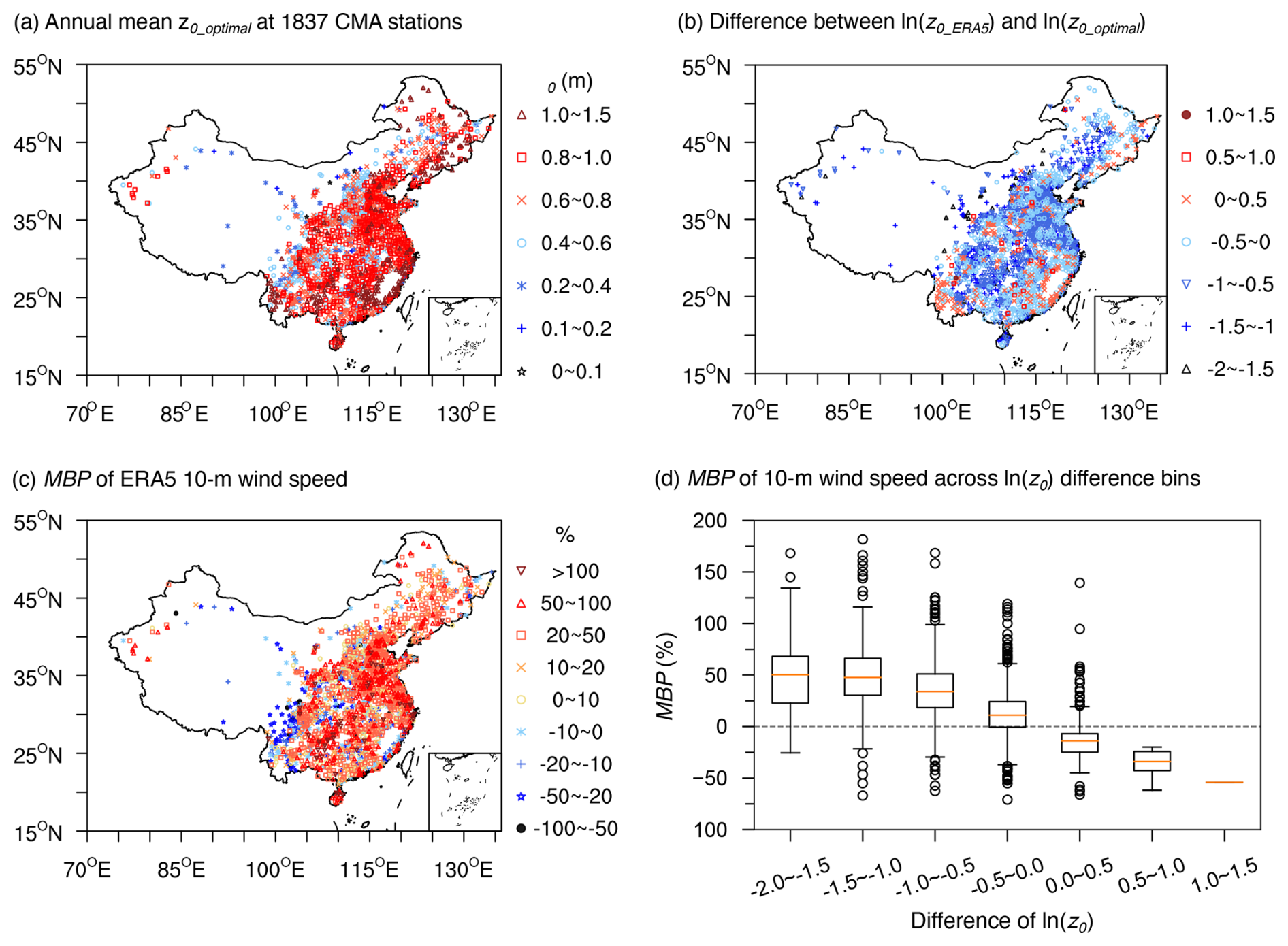
Figure 1 (a) Spatial distribution of annual mean z_{0_optimal} across 1837 CMA stations. (b) Difference between annual mean ln (z_{0_ERA5}) and ln (z_{0_optimal}) (i.e., ln (z_{0_ERA5}) minus ln (z_{0_optimal})). (c) MBP of 10 m wind speed between ERA5 and CMA stations. (d) Boxplots illustrating the statistical distribution of the MBP for 10 m wind speed shown in (c) across different intervals of ln (z₀) difference shown in (b).

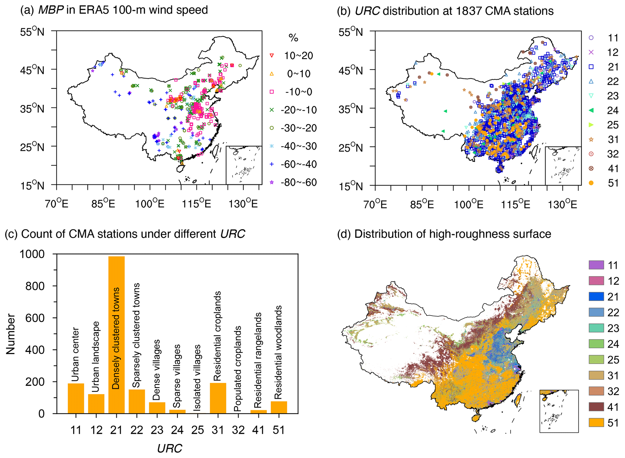
Figure 2 (a) MBP of 100 m wind speed between ERA5 and 589 anemometer towers. (b) Spatial distribution of urban-rural classification (URC) at 1837 CMA stations. The legend on the right indicates the URC codes, with the corresponding URC types labeled in panel (c). (c) Number of CMA stations for each URC. The numerical labels on the x axis represent the URC codes, with the specific URC types annotated on the bars. (d) Spatial distribution of high-roughness surface areas, which are composed of the 11 types covered by CMA stations in panel (b).

Additionally, as a consistency check, we examined how the difference in ln (z₀) covaries with the 10 m wind-speed bias between ERA5 reanalysis and station observations. Compared to the annual mean ln (z_{0_optimal}) derived from 1837 stations, the ln (z_{0_ERA5}) values are systematically lower at most locations, resulting in positive MBP values of 10 m wind speed between ERA5 reanalysis data and station observations (Fig. 1b and c). The discrepancies between ln (z_{0_ERA5}) and ln (z_{0_optimal}) are likely due to rapid urbanization around the majority of CMA stations, characterized by extensive construction of buildings, which enhances surface roughness and consequently reduces near-surface wind speeds (Li et al., 2018; Zhang and Wang, 2021). However, the impact of urbanization is likely not considered in the ERA5 reanalysis. Figure 2b and c depicts the distribution of CMA stations classified by urban-rural categories. All stations are situated in high-roughness surface areas, with the majority located in urban and town regions, highlighting the need to incorporate urbanization effects into wind speed simulations to improve model accuracy. In contrast, at a few locations, where the ln (z_{0_ERA5}) values are higher, the corresponding MBP values of 10 m wind speed are negative (Fig. 1b and c). The influence of ln (z₀) difference on wind speed bias becomes more pronounced as the magnitude of ln (z₀) deviation increases (Fig. 1d). Because ln (z_{0_optimal}) is defined as a monthly median of hourly ln (z₀), this cross-time statistic does not trivially inherit the instantaneous relationship implied by Eqs. (1)–(3). The monotonic, theory-consistent pattern observed in the binned ln (z₀) difference versus wind-speed MBP therefore serves as a post-aggregation consistency check, rather than as proof. Accordingly, the robust consistency in the relationship between z₀ and wind speed preliminarily supports that z_{0_optimal} is reasonable, and suggests that improving z₀ values over high-roughness surface areas in numerical models could significantly enhance wind speed simulation accuracy. The validity of z_{0_optimal} will be assessed via independent validation by comparing simulated wind speeds with observations (Sect. 3.3).

3.2 Development of a gridded z₀ dataset in high-roughness surface areas across China

To demonstrate the reliability and practicality of the estimated z_{0_optimal}, we constructed a gridded z₀ dataset based on these estimations in order to apply it in numerical simulations. Given that the estimated z₀ values from 1837 stations are located within high-roughness surface areas consisting of 11 distinct types (Fig. 2b and c), this study developed a monthly gridded z₀ dataset specifically for these categories of areas with a spatial resolution of 0.01°×0.01° using the RFR algorithm, referred to as z_{0_RFR}. As a representative example, the z_{0_RFR} dataset was generated for the year 2019, and its spatial coverage is shown in Fig. 2d. Although 2019 was chosen for demonstration, the RFR model itself is year-independent and can be applied to other years, provided that the required input features are available. Six feature variables closely related to z₀ were used as inputs, encompassing topographic characteristics ($\stackrel{\mathrm{‾}}{{\mathit{\theta }}^{\mathrm{2}}}$ and TSD), vegetation conditions (PTC, LAI, and NDVI), and urban-rural distribution (URC).

Figure 3c shows that the RFR algorithm exhibits satisfactory performance on both training and test subsets. Feature importance analysis reveals that topographic features and PTC exert the most significant influence on ln (z_{0_RFR}) (Fig. 3e). z₀ is primarily controlled by the characteristic height of surface roughness elements, particularly their relief. Consequently, topographic features rank among the most influential factors. For vegetation-related features, PTC not only reflects the horizontal distribution of vegetation density but also serves as a proxy for the presence of tall roughness elements. By contrast, LAI mainly represents vegetation density, making it relatively less critical. Although LAI is strongly correlated with NDVI (R=0.72), its low importance is not driven by this collinearity. The URC ranks only fourth in feature importance. This ranking should not be interpreted as implying that land use or urbanization is insignificant. Rather, in our framework, URC is used mainly to delineate the study domain and to ensure that the RFR algorithm is applied only to high-roughness surface areas. The aerodynamic effects of high-roughness elements, such as tall vegetation, buildings, and other infrastructure, are already embedded in the wind observations from CMA stations. As a result, the influence of these roughness elements is directly reflected in the z₀ values themselves, rather than being captured by the URC. Essentially, URC is not defined in terms of the morphological height and density of roughness elements; instead, derived from global land-cover and population data (Li et al., 2023), and therefore z₀ is weakly sensitive to URC. For example, in categories of Urban center and Urban landscape, there remains non-negligible tree cover, mean tree fractions of approximately 10 % and 11 %, respectively (Fig. S1b). This lowers URC's ranking in feature-importance analyses. To better capture the influence of roughness elements, more detailed surface parameters, such as building height and building density, would be helpful. Once such data are widely accessible, they should be incorporated to further improve the accuracy of z₀ estimates.

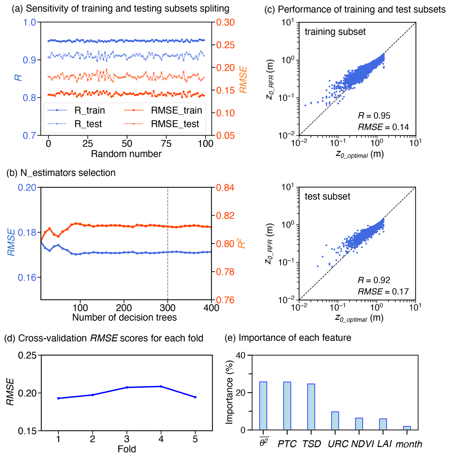
Figure 3 Sensitivity analysis and performance evaluation of the Random Forest Regression (RFR) algorithm. (a) Sensitivity of RFR results to the randomization seed for training and test subsets splitting. R and RMSE represent correlation coefficient and root mean square error, respectively. (b) Determination of the optimal number of decision trees. R² represents determination coefficient. (c) Performance of the RFR algorithm on the training and test subsets. The R and RMSE values are displayed. (d) Performance evaluation using five-fold cross-validation. (e) Importance scores of different feature variables.

The spatial distribution of ln (z_{0_RFR}) shows limited monthly variability (Fig. S2). The most pronounced monthly variations occur predominantly in the northern regions, likely because these areas exhibit strong seasonal changes in vegetation structure and biomass. The annual mean spatial distribution of z_{0_RFR}, with values in high-roughness surface areas generally falling within the range of 0.3 to 0.9 m, exhibits distinct patterns compared to z_{0_Default} and z_{0_Peng} (Fig. 4a). In comparison with z_{0_Default} and z_{0_Peng}, z_{0_RFR} shows a more homogeneous spatial distribution pattern across China. Specifically, in northern China, z_{0_RFR} values are consistently higher than those of both z_{0_Default} and z_{0_Peng}, with z_{0_Default} generally higher than z_{0_Peng}. Conversely, in southern China, z_{0_Peng} values are significantly higher than both z_{0_Default} and z_{0_RFR}. However, in southeastern and southwestern China, z_{0_Default} values exceed those of z_{0_RFR}, while in the remaining southern areas, z_{0_RFR} maintains higher values compared to z_{0_Default}.

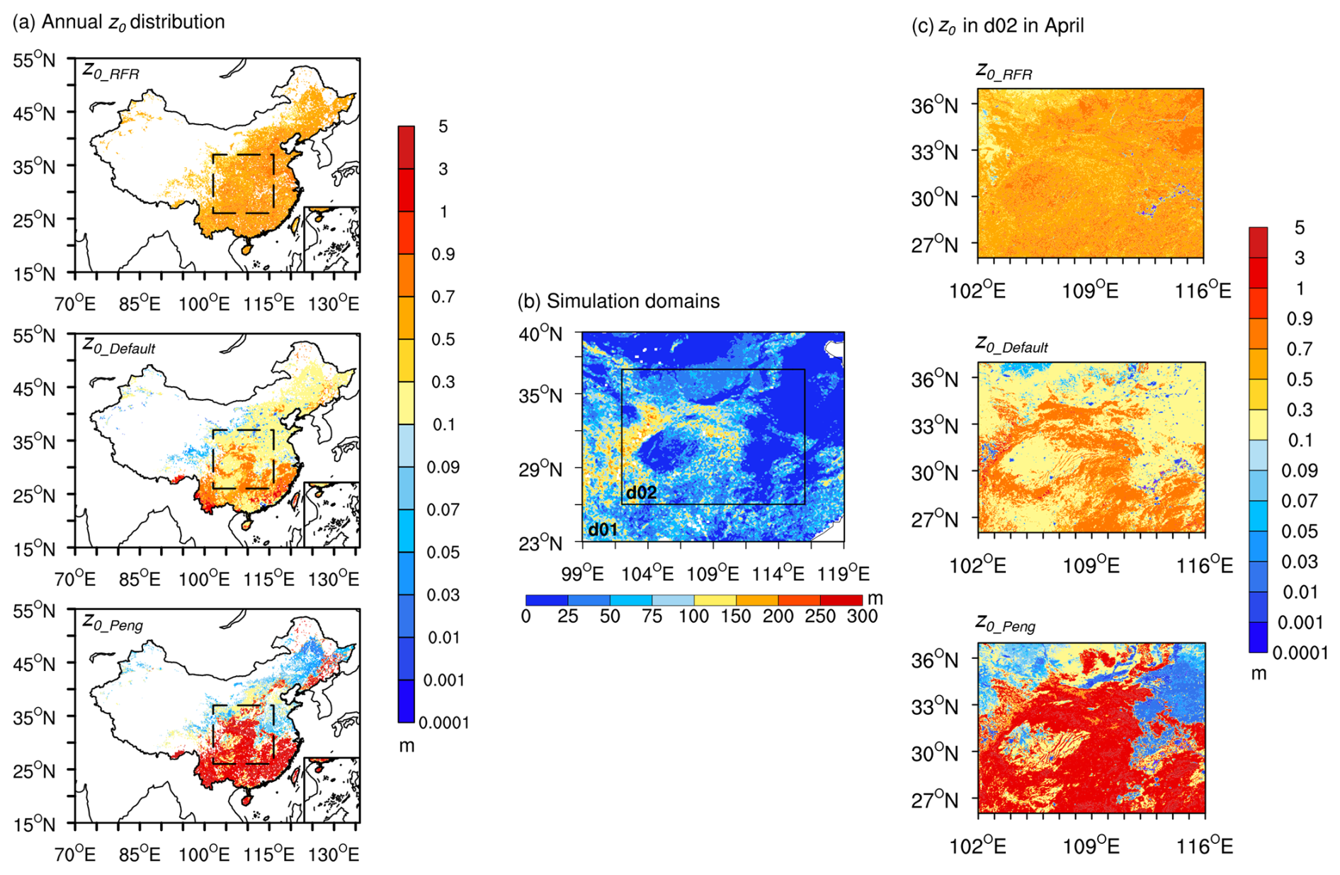
Figure 4 (a) Spatial distributions of annual mean z_{0_RFR}, z_{0_Default}, and z_{0_Peng}. The dashed rectangular box indicates the simulation domain (d02) in panel (b). (b) Nested simulation domains (d01: outer domain; d02: inner domain) with terrain standard deviation within 0.01° window (TSD) represented by color shading. (c) Spatial distributions of z₀ used in simulations over d02 in April.

3.3 Application of the produced z₀ dataset in wind speed simulation

To evaluate the performance of z_{0_RFR}, we implemented it in the WRF model for wind speed simulations, as z₀ directly affects near-surface wind speed. A ∼3 km simulation for April 2019 was conducted using the WRF model with z_{0_RFR} over the regions outlined in Fig. 4a, which correspond to the d02 domain in Fig. 4b and represent the primary areas of z_{0_RFR} concentration. April was selected because it is the month with the highest average wind speed in the target domain (Fig. S3), thus better reflecting the impact of z₀ on wind speed. For comparison, two additional simulations were performed: one utilizing the WRF model's default roughness length (z_{0_Default}) based on land cover types, and the other employing a recent z₀ dataset (z_{0_Peng}). In the northeastern, northern, and western regions of the d02 domain, both z_{0_Default} and z_{0_Peng} are generally lower than z_{0_RFR} estimates, with z_{0_Peng} having even lower values than z_{0_Default} (Fig. 4c). However, this pattern reverses in the southeastern areas and along the surrounding area of the Sichuan Basin, where both z_{0_Default} and z_{0_Peng} surpass z_{0_RFR} estimates, and notably, with z_{0_Peng} having significantly higher values than z_{0_Default} in these regions. These discrepancies in z₀ would inevitably directly affect the accuracy of wind speed simulation. To evaluate the influence, we conducted a comprehensive assessment on both 10 and 100 m wind speed simulations, which represent typical heights for meteorological observations and wind energy applications, respectively.

3.3.1 Evaluation of the simulated 10 m wind speed

We first compared the simulated 10 m wind speed with observations from 753 CMA stations in study areas (d02 domain), showing that z_{0_RFR} significantly enhances the accuracy of simulations. The improvement due to z_{0_RFR} is evident in the smaller MBP values of the simulated wind speed (Figs. 5a and S4) and the closer alignment of average wind speed with observational data (Fig. 6a).

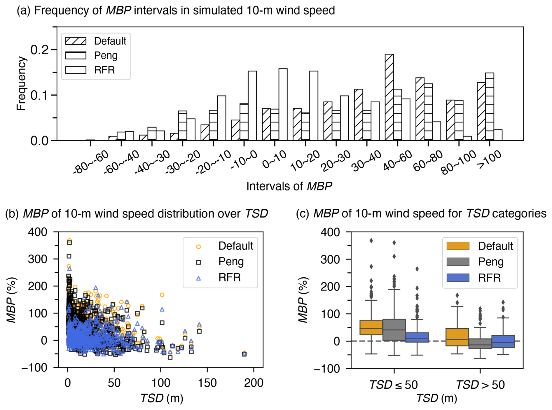
Figure 5 (a)  z_{0_Default}, z_{0_Peng}, and z_{0_RFR} against observations from CMA stations. (b) Distribution of MBP in 10 m wind speed as a function of TSD. (c) Box plot of MBP in 10 m wind speed across different TSD bins.

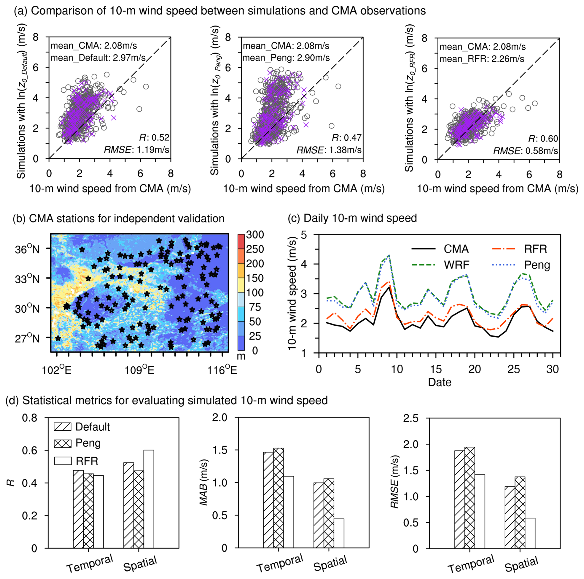
Figure 6 (a) Comparisons of mean 10 m wind speed in April between the simulations using z_{0_Default}, z_{0_Peng}, and z_{0_RFR} versus observations from CMA stations. All points (grey circles and purple crosses) represent the 753 CMA stations within the d02 domain available for comparison, while the purple crosses represent the 148 stations utilized for independent validation, which were not used in training the z_{0_RFR} model. The corresponding wind speed means, R, and RMSE of all stations are also indicated. (b) Distribution of the 148 independent CMA stations (black stars). Colored shaded areas represent TSD. (c) Comparison of daily mean 10 m wind speed between simulations and observations from 753 CMA stations. (d) Statistical metrics comparing simulated and observed 10 m wind speeds, including temporal and spatial R, MAB, and RMSE.

Specifically, the frequency histogram of MBP values reveals that the simulation results using z_{0_RFR} mostly fall within an absolute MBP range of less than 30 %, with a substantial proportion concentrated below 10 %. In contrast, simulations employing z_{0_Default} display a majority of MBP values exceeding 30 %, while simulations using z_{0_Peng} are even poorer, with a larger number of stations falling within higher MBP ranges (Fig. 5a). The improvement in 10 m wind speed induced by z_{0_RFR} is primarily evident in relatively flat regions. As TSD increases, the improvement gradually diminishes (Fig. 5b). z_{0_RFR} outperforms both z_{0_Default} and z_{0_Peng} when TSD does not exceed 50 m, while it shows superior performance to z_{0_Default} and comparable results to z_{0_Peng} when TSD is greater than 50 m (Fig. 5c). Spatially, significant improvements are observed in the relatively flat eastern and northern study areas, whereas limited enhancements are found in regions with higher TSD surrounding the Sichuan Basin (Fig. S4). The limited improvement in relatively complex terrain arises because, in addition to z₀, wind speed over these regions is influenced by multi-scale factors, including microscale terrain features (Ge et al., 2025), turbulent orographic form drags (Beljaars et al., 2004; Jiménez and Dudhia, 2012; Zhou et al., 2018), surface heating-induced mountain-valley circulations (Kim et al., 2021), mountain waves (Draxl et al., 2021) and other processes. Inaccurate parameterizations of these factors in numerical models can all lead to errors in wind speed simulations.

Table 1 Mean 10 m wind speed at 753 CMA stations and mean 100 m wind speed at 50 anemometer towers from simulations and observations. Simulations were performed using z_{0_Default}, z_{0_Peng}, and z_{0_RFR}. Also shown is the percentage reduction in wind speed error (PRE) achieved by z_{0_RFR} relative to z_{0_Default} and z_{0_Peng}.

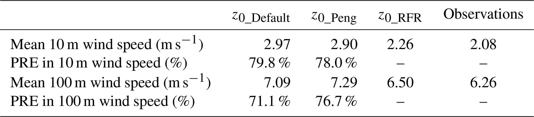
For the mean 10 m wind speed, simulations using z_{0_RFR} (2.26 m s⁻¹) show better agreement with the CMA observations (2.08 m s⁻¹), whereas simulations with z_{0_Default} and z_{0_Peng} show greater overestimations, producing mean wind speeds of 2.97 and 2.90 m s⁻¹, respectively (Fig. 6a and Table 1). In other words, z_{0_RFR} decreases mean bias of 10 m wind speed by 79.8 % and 78.0 % compared to z_{0_Default} and z_{0_Peng}, respectively. Independent validations across 148 stations (Fig. 6b), from the test subset in the generation of z_{0_RFR}, further confirm the superiority of z_{0_RFR} (Fig. 6a). In addition, the improvements in 10 m wind speed were observed throughout the entire simulation period (Fig. 6c). Note that our experimental design, employing a re-initialization strategy, means that 30 independent simulation experiments were conducted in April. Thus, although the simulations were only conducted for a month, the consistent improvement across all days shows that the enhancement achieved by z_{0_RFR} is robust. Moreover, the statistical metrics also show that the simulated 10 m wind speed using z_{0_RFR} outperforms those using z_{0_Default} and z_{0_Peng} in temporal and spatial MAB and RMSE (Fig. 6d).

3.3.2 Evaluation of the simulated 100 m wind speeds

In addition to 10 m wind speed, the simulated 100 m wind speed was also improved through the use of z_{0_RFR} (Fig. 7a and Table 1). Compared to observations from 50 anemometer towers (Fig. 7b), with an average 100 m wind speed of 6.26 m s⁻¹, simulations based on z_{0_Default} and z_{0_Peng} overestimate the wind speed, with averages of 7.09 and 7.29 m s⁻¹, respectively. However, the mean 100 m wind speed simulated using z_{0_RFR} is 6.50 m s⁻¹, closer to the observations (Table 1). This improvement using z_{0_RFR} reduces wind speed mean bias by 71.1 % and 76.7 % compared to z_{0_Default} and z_{0_Peng}, respectively. Consistent with the performance of z_{0_RFR} at 10 m wind speed, the improvement in 100 m wind speed is more pronounced in relatively flat regions (Fig. 7c). The outliers in Fig. 7a, where wind speed biases remain significant despite using z_{0_RFR}, are located in areas with higher TSD. Furthermore, similar to its performance at 10 m height, z_{0_RFR} demonstrates superior performance in simulated 100 m wind speed across both temporal and spatial metrics, with the exception of the temporal correlation coefficient (Fig. 7d). The relatively lower temporal R is reasonable, as the improvement in wind speed induced by z₀ primarily stems from enhancements in the vertical profile.

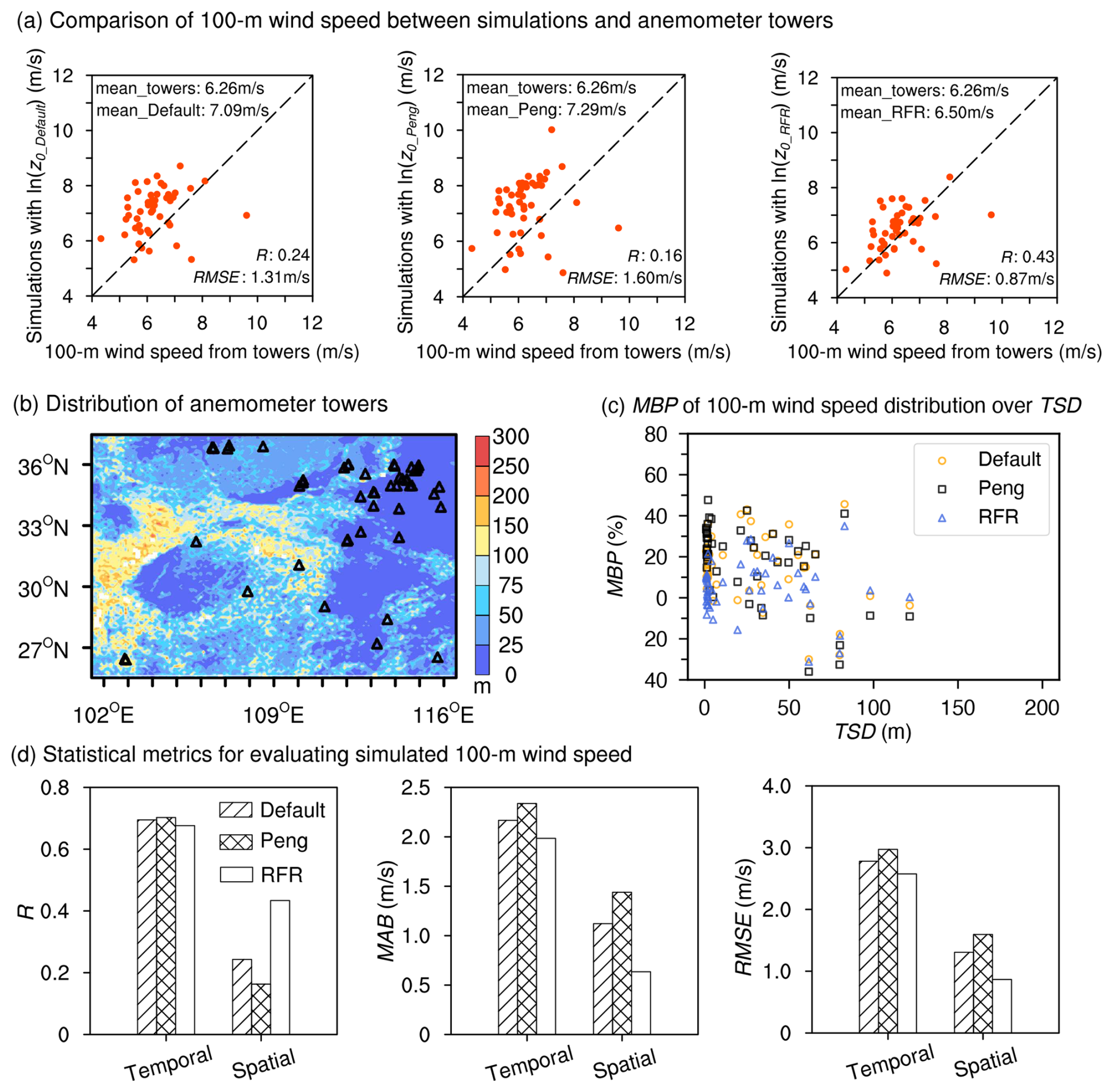
Figure 7 (a) Comparisons of mean 100 m wind speed in April between the simulations using z_{0_Default}, z_{0_Peng}, and z_{0_RFR} versus observations from anemometer towers. The corresponding wind speed means, R, and RMSE of all towers are also indicated. (b) The locations of 50 anemometer towers (black triangles) utilized for 100 m wind speed evaluation. Colored shaded areas represent TSD. (c) Distribution of MBP in 100 m wind speed as a function of TSD. (d) Statistical metrics comparing simulated and observed 100 m wind speeds, including temporal and spatial R, MAB, and RMSE.

In summary, the 30 independent simulation cases conducted for April demonstrate that the z₀ values derived from the combination of CMA observations and ERA5 data are highly reliable. The resulting gridded z₀ dataset significantly reduces uncertainties in mesoscale near-surface wind speed simulations, particularly over relatively flat high-roughness surface areas. To further validate the robustness of the z₀ estimation method and the resulting dataset, we conducted additional simulations for October 2019, a month characterized by generally weaker wind conditions (Fig. S3), using the same model configuration as in April. The results (Figs. S5–S7) also show consistent improvements when using z_{0_RFR}. Station-wise correlations increase and errors decrease to a similar extent in both months, and the daily time series likewise show closer tracking of peaks and lulls. Taken together, these results further reinforce the reliability and applicability of the proposed z₀ estimation under varying meteorological conditions. They also indicate that although phenology-driven changes in canopy structure and seasonal circulation modulate wind speeds, the performance advantage of the proposed z₀ is not diminished.

4 Discussion

Here we discuss the sensitivity and generality of the site z₀ estimation approach with respect to the input simulation or reanalysis data, addressing concerns about potential methodological dependence on ERA5. Our study utilized ERA5 reanalysis data and CMA observations for initial z₀ estimation. Compared to traditional meteorological or morphological methods, our approach can provide z₀ values at large spatial coverage and low cost, and these values lead to clear improvements in WRF-simulated wind speeds at both 10 and 100 m above ground level. To assess whether the performance gain stems from improved z₀ representation rather than from alignment with ERA5 reanalysis data, we carried out two additional sets of evaluations.

First, we applied the same approach to estimate z₀ from WRF-simulated 10 m wind speed and the model's default z₀ values (0.03°×0.03°), instead of ERA5. The z₀ values estimated using this alternative dataset were found to be highly similar to those derived from ERA5 (Fig. 8), indicating that the method is not inherently reliant on ERA5 as a data source. The primary advantage of using ERA5 lies in its extensive spatiotemporal coverage, which offers greater convenience and consistency with observational data. Meanwhile, although 10 and 100 m winds over lands are not assimilated directly in ERA5, its 4D-Var system ingests a wide range of surface and upper-air observations that constrain boundary-layer structure and indirectly improve near-surface winds; this strengthens the credibility of using ERA5 as the reference field (Hersbach et al., 2020). However, the methodology itself is general and transferable to other datasets.

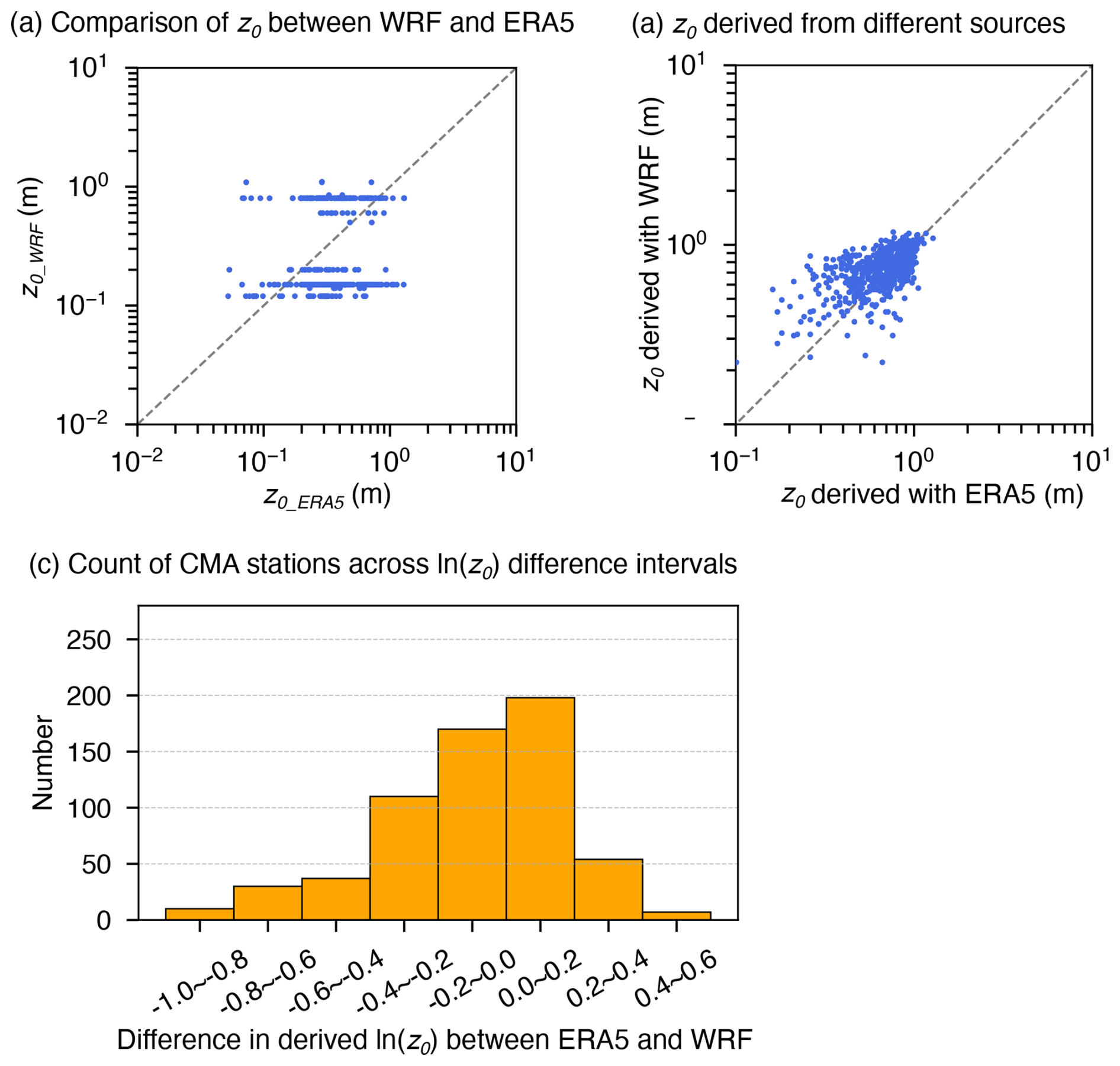
Figure 8 (a) Comparison of z₀ values from default WRF model (z_{0_WRF}) and ERA5 (z_{0_ERA5}). (b) Comparison of z₀ estimates using different datasets. z₀ derived from WRF represents the estimated values based on WRF simulations (10 m wind speed and default z₀) and CMA station observations (10 m wind speed) during April 2019, while z₀ derived from ERA5 denotes the estimates obtained in this study using ERA5 reanalysis data in April. (c) Distribution of station counts across intervals of the difference in derived ln (z₀) (ln (z₀) derived from ERA5 minus ln (z₀) derived from WRF).

Moreover, the agreement between ERA5- and WRF-derived z₀ values suggests that the spatial extent represented by the estimated site-level z₀ values is not determined by the resolution of the reanalysis or simulation dataset used, but rather by the measurement height of wind observations at the stations. In this study, 10 m wind speeds from CMA stations were used. As a rule of thumb, the horizontal representativeness of wind measurements is approximately 10–100 times the measurement height. Therefore, z₀ values estimated from 10 m wind observations are reasonably representative at ∼100 m–1 km scales, making the generation of 0.01° gridded z₀ datasets for use in mesoscale simulations both appropriate and justified, with no evident resolution dependence observed. We compared simulation results at different resolutions. Leveraging the nested modeling setup used in this study, the d01 domain with a 0.09° resolution was treated as the coarse-resolution simulation, while d02 at 0.03° served as the fine-resolution simulation. The results show that, even at the coarser resolution, our gridded z₀ dataset provides a clear advantage and substantially improves near-surface wind speed simulations (Figs. S8 and S9). However, for simulations at ∼1 km resolution and finer, such as urban-scale wind modelling, our z₀ dataset cannot fully capture urban heterogeneity, because it did not incorporate key morphological parameters (e.g., building height and density) to distinguish between different urban forms. Therefore, an urban canopy model (UCM) would be a more appropriate choice. UCMs were conceived to operate at ∼0.5–1 km grid spacing to bridge mesoscale forecasting (∼10⁵ m) with microscale transport/dispersion (∼10⁰ m) models (Tewari et al., 2006; Chen et al., 2011), and they have been widely applied and validated in subsequent urban studies (Lian et al., 2018; Salamanca et al., 2018; Wang and Hu, 2021). Therefore, our z₀ data are suitable and effective for mesoscale simulations at kilometer-level resolutions.

Second, we further validated the robustness of the refined z₀ dataset (z_{0_RFR}) by conducting additional WRF simulations driven by the reanalysis from National Centers for Environmental Prediction (NCEP) instead of ERA5. These results (Fig. S10 and Table S1 in the Supplement) still showed significant improvement in wind speed simulation performance when using z_{0_RFR}, consistent with those driven by ERA5. This cross-reanalysis consistency demonstrates that the benefits are attributable to the improved surface representation through z_{0_RFR} refinement, not simply tuning to match ERA5-driven wind fields.

Taken together, these findings confirm that the z₀ estimation method proposed in this study is robust, flexible, and not dependent on alignment with a specific reanalysis dataset. It provides a practical framework for z₀ estimation that can be widely applied across different reanalysis/simulation datasets and observational data with consistent benefits. However, this method is limited in regions with sparse or no surface weather stations. Notably, these regions, such as western and northern China, are rich in wind resources and are key targets for wind energy development. Therefore, producing high-quality gridded z₀ datasets in these regions warrants further study by exploring alternative data sources, such as anemometer tower wind profiles, to supplement z₀ truth values (Wang et al., 2024).

The two assumptions used in the z₀ estimation are also discussed. Although these assumptions cannot be fully verified with the available data, they are pragmatically motivated and indirectly supported by the improved performance of wind-speed simulations using the resulting z₀ estimates. Assumption 1 posits that the near-surface wind-speed discrepancy between ERA5 reanalysis and CMA observations is dominated by z₀ and that the influence of z₀ weakens with height, making ERA5 winds at higher levels within the surface layer comparable to observations. This is partly supported by the spatial pattern of estimated z₀ (denser over eastern China, where 100 m wind-speed biases between ERA5 reanalysis and anemometer tower observations are smaller; Figs. 1c and 2) and by a sensitivity test on the reference height (Fig. S11a and c). When re-estimating annual-mean z_{0_CMA} at 150 and 200 m, most stations show an absolute difference from the 100 m-based estimate below 0.2, indicating broad consistency across heights. A minority of stations exhibit slightly larger deviation, which may be influenced by local terrain complexity (Fig. S11b and d). Assumption 2 treats the effects of atmospheric stability on wind speed as effectively similar in ERA5 and at CMA sites, allowing us to omit explicit stability corrections in estimating z_{0_CMA}. This simplification enhances methodological consistency and computational efficiency, and it is indirectly supported by the validation of simulated winds. Moreover, prior work has shown that neutral log-law method can perform comparably to stability-corrected scheme for vertical interpolation in US wind-resource assessments (Duplyakin et al., 2021), suggesting that such an approximate treatment seems feasible and a widely adopted simplification. Overall, although neither assumption can be fully verified with the presently available data, their practical applicability is evidenced by improved WRF wind-speed simulations. Future work, ideally leveraging multi-height wind profile observations and coincident stability metrics could further test these assumptions, yield more precise z₀ estimates.

5 Conclusion

The representation of z₀ in numerical models, typically determined by land cover types, may lead to significant uncertainties in wind speed simulations and predictions. Traditional methods for obtaining z₀ ground truth are mainly constrained by high costs. In this study, we proposed a low-cost z₀ estimation method, allowing the acquisition of z₀ values at routine weather stations.

Specifically, this approach leverages 10 m wind speed and z₀ values from ERA5 reanalysis data, along with observed 10 m wind speeds at CMA stations, to derive optimal z₀ at stations by minimizing the difference in 100 m wind speeds between reanalysis and observations. Here, the 100 m wind speed is expressed with 10 m wind speed and z₀ using similarity theory. Based on this approach, we derived z₀ values at 1837 CMA stations out of a total of 2161 stations. These stations are located in high-roughness surface regions, indicating the estimated z₀ values inherently include the effects of built-up and tall vegetation.

To validate the reliability and practicality of the estimation method, we utilized a Random Forest Regression algorithm, incorporating feature variables closely related to z₀, to develop a monthly gridded z₀ dataset for high-roughness surface areas in China with a spatial resolution of 0.01°×0.01°. The resulting ln (z₀) values mainly range from −1 to 0. Simulations with WRF model show that, compared to the default z₀ in WRF and a recent gridded z₀ dataset developed by Peng et al. (2022), the z₀ dataset constructed in this study has significantly improved the accuracy of near-surface wind speed simulations in high-roughness surface areas, particularly in relatively flat regions. Evaluations against weather station data and anemometer tower data show simulations with the new z₀ dataset mitigate mean bias of 10 m wind speed by 79.8 % and 78.0 %, and mean bias of 100 m wind speed by 71.1 % and 76.7 %, respectively, compared to the default z₀ in WRF and the z₀ dataset from Peng et al. (2022).

In summary, this study developed a simple yet effective approach for correcting model z₀, addressing the limitations of relying on empirical values assigned based on land cover types. The method shows particular effectiveness in z₀ correction for high-roughness surface areas and offers valuable support for wind field-dependent studies and applications.