Assimilation of snow water equivalent from AMSR2 and IMS satellite data utilizing the local ensemble transform Kalman filter

Snow water equivalent (SWE), as one of the land initial or boundary conditions, plays a crucial role in global or regional energy and water balance, thereby exerting a considerable impact on seasonal and subseasonal-scale predictions owing to its enduring persistence over 1 to 2 months. Despite its importance, most SWE initialization remains challenging due to its reliance on simple approaches based on spatially limited observations. Therefore, this study developed an advanced SWE data assimilation framework with satellite remote sensing data utilizing the local ensemble transform Kalman filter (LETKF) and the Joint UK Land Environment Simulator (JULES) land model. This approach constitutes an objective method that optimally combines two previously unattempted incomplete data sources: the satellite SWE retrieval from the Advanced Microwave Scanning Radiometer 2 (AMSR2) and dynamically balanced SWE from the JULES land surface model. In this framework, an algorithm is additionally considered to determine the assimilation process based on the presence or absence of snow cover from the Interactive Multisensor Snow and Ice Mapping System (IMS) satellite, renowned for its superior reliability.

The baseline model simulation from JULES without satellite data assimilation shows better performance in high-latitude regions with heavy snow accumulation but is relatively inferior in the transition regions with less snow and high spatial and temporal variation. Contrastingly, the AMSR2 satellite data exhibit better performance in the transition regions but poorer performance in the high latitudes, presumably due to the limitation of the satellite data in the penetrating depth. The data assimilation (DA) demonstrates the positive impacts by reducing uncertainty in the JULES model simulations in most areas, particularly in the midlatitude transition regions. In the transition regions, the model background errors from the ensemble runs are significantly larger than the observation errors, emphasizing great uncertainty in the model simulations. The results of this study highlight the beneficial impact of data assimilation by effectively combining land surface model and satellite-derived data according to their relative uncertainty, thereby controlling not only transitional regions but also the regions with heavy snow accumulation that are difficult to detect by satellite.

1 Introduction

Snow plays a crucial role in regulating the water, energy, and carbon exchange between the land surface and atmosphere (e.g., Dutra et al., 2011; Thomas et al., 2016). A snowpack tends to increase surface albedo and soil moisture as the snow melts (Eagleson, 1970), thereby affecting the climate system through changes in water and energy balances. In addition to local impacts, the continental snowpack over Eurasia can influence the large-scale atmospheric circulation during winter (e.g., Li and Wang, 2014) or in spring (e.g., Broxton et al., 2017). Eurasian autumn snow in particular can affect upward-propagating stationary Rossby-wave activity, leading to stratospheric warming and weakening of the stratospheric polar vortex and jet stream, which in turn emerges as a negative Arctic oscillation (AO)-like pattern at the surface during winter due to downward propagation through the troposphere. Its impact is shown in both observation and model experiments (e.g., Allen and Zender, 2011; Cohen et al., 2007). Furthermore, the interannual variability of snow melting during the boreal spring season affects surface soil moisture in summer, which has important implications for heatwave development and emphasizing mechanisms through land–atmosphere interactions (Seo et al., 2020).

On subseasonal to seasonal (S2S) timescales, land initial states are crucial components in the S2S timescale predictions due to the inherent memory that changes slowly for 1 to 2 months in the climate system (e.g., Derome et al., 2005; Chen et al., 2010; Seo et al., 2019). In particular, the realistic snow initial states contribute to improving S2S prediction skills, as proven in several modeling studies. For example, previous studies (Orsolini et al., 2013; Jeong et al., 2013) demonstrated a considerable enhancement in the prediction skill of 2 m air temperature up to a lead time of 1–2 months across certain regions of Eurasia and the Arctic during winter, depending on snow initialization. Moreover, other studies (Orsolini et al., 2016; Li et al., 2019) have revealed that wave activity propagating toward the stratosphere, influenced by snow initial conditions in climate models, can induce changes in the polar vortex and contribute to the persistence of the North Atlantic Oscillation (NAO) and the AO. This emphasizes the significance of snow initialization in climate models as an essential process for enhancing prediction performance at the S2S timescales.

Snow states, i.e., snow water equivalent (SWE) used directly for hydrological analysis and initial states of the model (Li et al., 2019; Gan et al., 2021), are generally provided from in situ observation data, remote sensing retrievals from satellites, or numerical models such as a land surface model (LSM) operated based on the observed atmospheric variables. For the in situ data snow depth (SD) measurements prevail, largely attributed to the challenges associated with acquiring precise SWE data (Takala et al., 2011; De Rosnay et al., 2014). Surface synoptic observations (SYNOPs) serve as the principal source of SD measurements. In situ measurements offer the most dependable snow information, yet they are characterized by relatively coarse temporal and spatial resolutions, particularly within limited areas, due to the spatial heterogeneity inherent in snow distribution (Helmert et al., 2018; Meyal et al., 2020). Satellite-derived observations using conical scanning microwave instruments may provide spatially consistent data coverage across the globe. Cho et al. (2017) showed the SWE retrieval results from two passive microwave sensors, the Advanced Microwave Scanning Radiometer 2 (AMSR2) and the Special Sensor Microwave Imager Sounder (SSMIS). However, the algorithms for SWE retrieval exhibit a degree of sensitivity to a variety of parameters such as snow liquid water content and snow grain size distribution (De Rosnay et al., 2014). Hence, satellite-based SWE data still have limitations in accuracy, especially under deep snow conditions due to the limited penetration depth (Gan et al., 2021). On the other hand, satellite retrieval can estimate snow cover accurately under clear-sky conditions (Brubaker et al., 2009). Model simulations obtained from LSMs and simple snow models can cover complete spatiotemporal resolution but involve potentially large uncertainties due to the deficiencies in the physical parameterizations and meteorological forcing data (Dirmeyer et al., 2006; Seo et al., 2021).

Considering that a snow observation dataset has its respective strengths as well as limitations, data assimilation or other data fusion methods can prove to be beneficial for constructing snow states such as reanalysis data (e.g., Brasnett, 1999; Dee et al., 2011; Meng et al., 2012; Pullen et al., 2011; De Rosnay et al., 2014). For example, the snow analysis for the Canadian Meteorological Center (CMC) utilizes a two-dimensional optimal interpolation (2D-OI) scheme with in situ observations and the outputs from a simple snow model (Brown et al., 2003). The National Centers for Environmental Prediction (NCEP) Climate Forecast System Reanalysis (CFSR) combines the multi-satellite-based Interactive Multisensor Snow and Ice Mapping System (IMS) as satellite-based snow cover retrieval and the outputs from the global snow model of the Air Force Weather Agency (Meng et al., 2012). At the European Centre for Medium-Range Weather Forecasts (ECMWF), the ECMWF reanalysis (ERA)-Interim and ERA5 for snow analysis employ a Cressman interpolation and 2D-OI, respectively, with the IMS, in situ observation, and the results from a land surface model (Dee et al., 2011; De Rosnay et al., 2014). The Japanese 55-year Reanalysis (JRA-55) also utilizes the 2D-OI with in situ observations, satellite-based snow cover from SSMIS, and the results from an LSM (Kobayashi et al., 2015). Given that the majority of the reanalysis datasets rely on snow depth measurements, the SWE estimation is likely to introduce potential accuracy concerns when the snow depth information is combined with the snow density calculations.

Climate prediction systems in operational centers such as the Meteorological Office (Met Office) in the United Kingdom and the Korean Meteorological Administration (KMA) conduct snow initialization by utilizing the results of the operational global Unified Model (UM) and the IMS snow cover, which solely indicates the presence of snow (Pullen et al., 2011) and is lacking in its ability to reflect the physical quantity of it. The initialization at NCEP also performs a similar approach using input data combined from IMS snow cover and results from the global SD model (SNODEP; Meng et al., 2012). Furthermore, the snow initialization of ECMWF employs optimal interpolation with a combination of results from the LSM, IMS snow cover, and in situ observations from SYNOPs and national networks available on the Global Telecommunication System (GTS). However, in regions where ground observations are unavailable, large errors may exist in the snow model outputs due to uncertainties in atmospheric forcing and imperfect model parameterization (Boone et al., 2004; Essery et al., 2009). Often, the snow processes parameterized in LSMs rely on observed properties sampled in limited areas (Lim et al., 2022). In addition, as IMS snow cover only identifies the presence of snow, data assimilation with satellite snow cover only is not sufficient and inappropriate in constraining water and energy conservation. Alternative methods that consider the physical quantity of snow are required for the snow initialization.

One approach to mitigate the spatial discontinuity of ground observations is to use satellite-derived SWE with wide spatial coverage and frequent temporal resolution. However, the SWE retrievals from satellites still have considerable uncertainties (De Lannoy et al., 2010; Dawson et al., 2018), which can arise from vegetation and terrain interference, sensor signal saturation, snowfall amount, and simplifications in the underlying assumptions of the retrieval algorithms (Liu et al., 2015). In particular, a region with heavy snow accumulation leads to a significant underestimation of SWE due to the limitations in penetration depth from satellites (Gan et al., 2021) so that satellite-derived SWE is not employed in the land initialization process. In previous studies, various approaches have been attempted to improve SWE product performance, such as combining satellite-derived SWE with ground observations (Pulliainen et al., 2020), different satellite datasets (Gan et al., 2021), simple snow models (Dziubanski and Franz, 2016), or LSMs (Kwon et al., 2017; Kumar et al., 2019). However, most previous studies have focused on targeted regions with limited ground-based observations. Snow initialization in global coverage using satellite-derived SWE remains a persistently challenging task.

Therefore, this study developed an advanced SWE data assimilation framework with satellite remote sensing data using the local ensemble transform Kalman filter (LETKF) and the Joint UK Land Environment Simulator (JULES) land model. While there are existing studies on SWE data assimilation (e.g., Oaida et al., 2019; Smyth et al., 2020; Luojus et al., 2021), the use of passive microwave observations based on the LETKF in this context is relatively rare (e.g., Girotto et al., 2020). This approach constitutes an objective method that optimally combines two previously unattempted incomplete data sources: the satellite SWE from the Advanced Microwave Scanning Radiometer 2 (AMSR2) and the dynamically balanced SWE from the JULES land model forced by observed atmospheric fields. The estimated SWE data exhibit better consistency by additionally using snow cover data from the IMS data. This assimilation framework also enables the assessment of improvement as it provides insights into the reasons behind the performance improvement based on the Kalman gain analysis that measures the relative significance of the input data between the satellite and the land model during the data assimilation cycle. The satellite data have demonstrated high reliability in the transition regions of climatologically shallow snow conditions (Gan et al., 2021), and these regions are known as “hot spots” of strong atmosphere–land coupling through snow melting and associated surface energy and water balance changes (Koster et al., 2004; Dirmeyer, 2011; Huning and AghaKouchak, 2020). From these perspectives, it would be important to evaluate the impact of satellites on the transition regions as well as on the deep accumulation regions where accurate satellite retrievals are challenging. Furthermore, the benefits of assimilating satellite retrievals in extremely high-temperature events, such as the case in April 2020 over Eurasia, can be elucidated. In this regard, we expect that this snow data assimilation framework with satellite-derived SWE can be significant in providing optimal snow initial states for improving the S2S prediction by global climate models.

2 Data and model

2.1 Satellite data

The snow information including snow cover and SWE can be derived from satellite measurements offering global coverage and high temporal as well as spatial resolution. For data assimilation, this study uses SWE calculated from brightness temperature measurements obtained by the AMSR2 on board the Japanese Aerospace Exploration Agency (JAXA) Global Change Observation Mission-Water (GCOM-W) satellite. This AMSR2 Unified Level-3 (L3) dataset offers daily estimation of SWE at 25 km resolution from July 2012 to the present. AMSR2 has a sensor designed to detect microwave radiation naturally emitted from the surface and atmosphere, employing six frequency bands ranging from 6.9 to 89 GHz. Through this conical scanning mechanism, AMSR2 can acquire day and night datasets with nearly constant spatial resolution over more than 99 % of the global coverage every 2 d. Comprehensive explanations of AMSR2 characteristics are available in Imaoka et al. (2010). AMSR2 is selected for the assimilation because it produces more accurate results by assimilating data from modern sensors (e.g., AMSR2) compared to data from conventional sensors (e.g., AMSR-E) (Cho et al., 2017).

The widely used multi-sensor-derived snow cover is IMS (e.g., Ramsay, 1998a; Helfrich et al., 2007) produced by the NOAA National Environmental Satellite Data and Information Service (NESDIS) for the Northern Hemisphere from February 2004 to the present at 4 km resolution. This dataset is generated using various data products, including multi-satellite images and in situ observations (U.S. National Ice Center, 2008). Since IMS provides binary (0: no snow, 1: snow-covered) snow cover information, we transform the IMS snow cover at 4 km grids to the snow cover fraction (SCF) within a 50 km LSM grid by counting the snow pixel number with a value of 1. A 50 km LSM grid is declared as snow-covered when more than 50 % of the 4 km pixels within the grid are covered with snow. In this study, the application of the assimilation process is determined based on IMS-based SCF, renowned for its superior reliability (e.g., Brown et al., 2014). Further details will be described in Sect. 3.3.

2.2 Reference data for SWE and SCF

The CMC daily estimated SWE is used for verification. The SWE data are processed using statistical interpolation between a background field derived from a simple snow model and in situ daily SD (Brown and Brasnett, 2010). In detail, this dataset utilizes optimal interpolation methods to acquire spatial SD from the in situ data, involving SYNOPs, special aviation reports from the World Meteorological Organization (WMO), and meteorological aviation reports (METARs). In areas with scant in situ data, a simple snow accumulation and melt model is employed to create an optimal interpolation that estimates snowmelt and snowfall worldwide, assuming the persistence of the snowpack mass between snowfall and melting events (Brasnett, 1999). Although the average elevation of snow measurement stations used in CMC is biased toward low elevations (<400 m), potentially causing relative negative biases at higher elevations with heavy snow accumulation, the CMC dataset is often considered the premier snow analysis accessible in the Northern Hemisphere (Su et al., 2010) and has still been widely used to evaluate model outputs (e.g., Reichle et al., 2011, 2017; Toure et al., 2018). Therefore, the SWE of CMC produced without the satellite-derived data is selected for verification as an independent dataset for evaluating the assimilated analysis with remote sensing snow retrievals. Since only daily SD analysis is provided in CMC, it is converted to daily SWE based on snow bulk density methods (e.g., Sturm et al., 2010). It is available from 12 March 1998 to the present and offers comprehensive coverage of the entire Northern Hemisphere with a horizontal resolution of 24 km. The SWE of CMC at its native horizontal resolution is interpolated onto the LSM grid through local area averaging.

2.3 JULES LSM

This study utilizes the JULES LSM from the Met Office (Best et al., 2011), a component land model of the Global Seasonal Forecasting System version 6 (GloSea6), which is a fully coupled atmosphere, ocean, land, and sea ice model. The surface types (or snow tiles) in the JULES LSM consist of four non-vegetated types (urban, land ice, inland water, and bare soil) and five vegetation functional types: C₃ temperate grass, needleleaf trees, shrubs, C₄ tropical grass, and broadleaf trees. For each surface tile, a separate energy balance is computed, and the average energy balance in the grid cells is determined by applying weights to the values of each surface tile. Two schemes are used within JULES to represent surface snow (e.g., Best et al., 2011; Burke et al., 2013). The simple method involves a zero-layer approach, which modifies the top soil level without using explicit model layers to represent snow processes. The other is the multi-layer approach, which is more comprehensive, as described in Best et al. (2011). In the case of vegetated surfaces, snow can be separated into ground snow and canopy snow or stored in a single effective reservoir. As both the zero-layer and multi-layer snow models provide similar results under various conditions (Best et al., 2011), this study used the zero-layer snow model with constant thermal conductivity and density for snow. Although the heat capacity of snow is ignored, the bulk thermal conductivity in the surface layer is reduced as the thermal conductivity of snow differs from that of the soil and the layer thickness increases. As long as snow persists on the ground, the skin temperature cannot exceed 0 °C, yet the heat flux utilized for melting the snow is diagnosed as the residual in the surface energy balance. The melted water is immediately drained from the snow and divided into runoff and soil infiltration, and liquid water is not stored or frozen in the snow. A detailed description of the energy and water cycling in the JULES LSM can be referenced in Best et al. (2011).

The prognostic variables (e.g., SWE) in the LSM are determined by meteorological forcing variables such as 2 m air temperature, humidity, 10 m wind speed, precipitation, surface pressure, and radiative fluxes. The 3-hourly JRA-55 reanalysis at 0.56° spatial resolution is employed for the meteorological forcing variables, which is linearly interpolated to the 50 km resolution of the LSM. The model background error needed for data assimilation is estimated by JULES ensemble runs with perturbed initial and boundary conditions. Following previous studies (Reichle, 2008; Seo et al., 2021), meteorological forcing variables are perturbed to account for the uncertainties in these variables, especially precipitation, downward shortwave, and downward longwave. Perturbations are applied using additive adjustments assuming a normal distribution for longwave radiation and multiplicative adjustments following a lognormal distribution for shortwave radiation and precipitation, as guided by previous studies (Seo et al., 2021). Here, the ensemble means of additional and multiplicative perturbations are zero and 1, respectively. The relationship between disturbed precipitation and radiative flux ensures the physical consistency among atmospheric forcing variables (Reichle, 2008). For instance, a negative anomaly in precipitation and downward longwave radiation is statistically linked to a positive anomaly of downward shortwave radiation. Detailed explanations regarding the perturbation of atmospheric forcings can be found in Reichle (2008).

3 Methodology

3.1 Bias correction

The discrepancy in SWE between remote sensing and LSMs often arises due to uncertainties in the model physics, forcing data, and satellite retrievals. These uncertainties can lead to a significant discrepancy in SWE between model simulations and satellite remote sensing retrievals, potentially degrading performance. In previous studies (e.g., Reichle and Koster, 2004; Seo et al., 2021), a scaling method of nonlinear cumulative distribution function (CDF) matching is used to account for the systematic bias of soil moisture in the model backgrounds. However, unlike soil moisture, SWE presents varying characteristics in the CDF distribution across different regions, such as between high and low latitudes, thus requiring the estimation of the distribution at each grid point. As a result, the insufficient sample size hinders the clear simulation of the CDF distribution, posing challenges in its application. To address this issue, we attempted to apply a simple and effective standard normal deviation scaling to satellite-derived SWE at each grid point, considering its potential use as initial conditions for JULES-LSM-based climate models. Based on the climatology and standard deviation for the model and remote sensing retrievals, the scaled SWE (O_new) from the satellite can be derived from the following relation:

$$\begin{array}{}\text{(1)}& O_{\mathrm{new}}=\left({\displaystyle \frac{O-\stackrel{\mathrm{‾}}{O}}{{\mathit{\sigma }}_{\mathrm{o}}}}\times {\mathit{\sigma }}_{\mathrm{m}}\right)+\stackrel{\mathrm{‾}}{M},\end{array}$$

where $\stackrel{\mathrm{‾}}{O}({\mathit{\sigma }}_{\mathrm{o}}$) and $\stackrel{\mathrm{‾}}{M}\left({\mathit{\sigma }}_{\mathrm{m}}\right)$ indicate the climatology (standard deviation) of remote sensing retrievals and the model, respectively. This approach has been widely utilized in observation-based land initialization and has proven to be effective (e.g., Koster et al., 2011; Jeong et al., 2013).

3.2 Data assimilation method

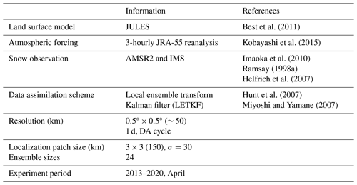
The snow assimilation is conducted based on the LETKF (e.g., Hunt et al., 2007), which is utilized to combine remotely sensed retrievals with the LSM outputs (also called backgrounds) at each grid point to produce a snow analysis. Unlike variational data assimilation methods, non-variational approaches (i.e., ensemble-based filters) characterize a probabilistic representation, with the spread of the ensemble serving as an estimate of forecast uncertainty. LETKF has several advantages over other data assimilation methods. First, LETKF can efficiently handle large datasets and high-dimensional state variables by localizing the covariance matrix. This offers efficiency in parallel computing, making it suitable for real-time forecasting and high-resolution data assimilation. In this study, the horizontal local patch size and the localization length scale parameters are defined as 150 and 30 km (Table 1), respectively. This approach involves the weight function for the covariance localization within the local patch centered at the analysis grid (e.g., Houtekamer and Mitchell, 2001; Hamill et al., 2001). This function assigns larger errors to observations located farther away from the center of the local patch, as proposed by Miyoshi and Yamane (2007), depending on the Gaussian function. Secondly, the method utilizes model simulation ensembles to capture the uncertainty in the initial states and background errors, which allows for a better representation of the flow-dependent probability distribution of the state variables that vary in time and space. Third, the LETKF employs an inflation parameter to adjust the ensemble spread, ensuring realistic uncertainty estimation by accounting for background errors. The underestimation of the analysis error covariance is typically issued by spatially and temporally constant boundary conditions as well as observation errors and limited ensemble members. Based on the standardized LETKF, this study applies a multiplicative covariance inflation of 20 % of the spread of 24 member ensembles for each data assimilation cycle. Furthermore, the Kalman gain analysis (Seo et al., 2021), which quantifies the ratio of the background error to the total error (equivalent to the sum of the background and the observation error), is conducted. This analysis serves to determine the weights assigned to assimilated observations in the analysis update processes of the LETKF.

Table 1 Description of the land surface model, the data used, and assimilation experiment designs.

3.3 Snow data assimilation design

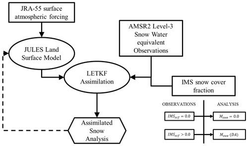
This study conducts the advanced daily cycle snow data assimilation experiment at each grid point using the LETKF based on the satellite data and the JULES LSM outputs driven by 3-hourly JRA-55 reanalysis atmospheric forcing. The snow assimilation processes are illustrated in Fig. 1, with a more detailed description in Table 1. Since data assimilation is conducted by considering the error of SWE in both the model and the observation, it is important to accurately understand the observation and background errors to improve the performance of data assimilation. The experiment calculates the background error from the 24 ensemble member spreads generated by perturbing atmospheric forcings such as longwave radiation, shortwave radiation, and precipitation in JULES LSM, as provided in Sect. 2.3. Due to the absence of precise error estimates for AMSR2 SWE retrievals, the observation error is conservatively prescribed as 10 % of AMSR2 SWE for each grid compared to the previous study utilizing AMSR2 SWE data (Lee et al., 2015), considering the general increase in errors during the snow accumulation period with the development of deep snowpack (Foster et al., 2005; Cho et al., 2017). Here, the bias-corrected AMSR2 satellite data as described in Sect. 3.1 are used as the observation data, and the updated snow analysis state through data assimilation becomes a new initial state for the next integration in JULES LSM (Fig. 1). In addition, the analysis state of this method is calculated based on the IMS snow cover fraction as follows (Fig. 1). If the SCF from IMS is 0, the snow analysis is set to zero; otherwise, it is derived through data assimilation. The reason for this is the importance of the presence or absence of snow in the climate system, as well as the high reliability of the IMS data (e.g., Brown et al., 2014). A background experiment using JULES LSM without satellite data assimilation as a baseline (referred to hereafter as “Openloop”) is also performed by employing the same ensemble perturbations, thereby measuring the skill improvement from the snow analysis state through the assimilation of satellite-derived SWE and IMS SCF from satellite and surface observations (referred to hereafter as “DA”). All experiments are conducted in April from 2013 to 2020, which is one of the months with low snow performance in the LSM when the snow begins to melt in the Northern Hemisphere (e.g., Toure et al., 2018; You et al., 2020).

Figure 1 Schematic diagram of the snow assimilation system with satellite-derived observations and the land surface model outputs.

4 Results

4.1 Skill verification

Figure 2 displays the climatological mean SCF from the IMS multi-satellite data (Brown et al., 2014) and the differences from IMS for AMSR2, Openloop, JRA-55, and DA for April 2013–2020. Here, the JRA-55 SCF serves as a reference dataset for comparison with other reanalyses and is associated with meteorological forcing data used in the JULES land surface model. April is a month when the accumulated snow during the cold season begins to melt. This study defines the transitional region with a climatological mean SWE of less than 16 mm as in previous studies (e.g., Gan et al., 2021); the boundary of these transition regions is represented by the black lines in Fig. 2. The transitional regions exhibit large variability in space and time, and they are mainly located at midlatitudes. The SCF climatology patterns show negligible differences in high latitudes of heavy snow accumulation but noticeable differences in the transitional midlatitude regions of less snow. SCF from JRA-55 tends to be underestimated compared to IMS, whereas AMSR2 and Openloop tend to overestimate. There is a clear difference in SCF between AMSR2 and IMS satellite data. This study gives more credibility to IMS than AMSR2, as the former is based on multiple satellite data sources (e.g., Brown et al., 2014). As we used the IMS SCF to define the snow region to be assimilated by AMSR2 SWE, it is natural that DA shows better consistency with IMS and reduces overestimation biases in Openloop. Quantitatively, the root mean square differences (accuracy, defined in Supplement Table S1 as in a previous study) for AMSR2, Openloop, JRA-55, and DA with (from) IMS are 0.23 (0.91), 0.18 (0.91), 0.13 (0.93), and 0.13 (0.97), respectively, showing the best consistency in DA. The quantitative differences between DA and other experimental results are minor, but noticeable spatial discrepancies exist, particularly around transition regions.

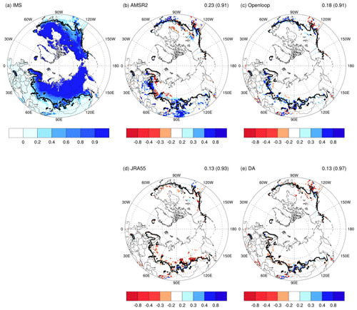
Figure 2 (a) Climatology of SCF from IMS used as a reference and (b–e) the differences from IMS for AMSR2, the baseline model simulation (Openloop), JRA-55, and the data assimilation (DA) results for April during 2013–2020. The black line represents the boundary of the transition region, defined as the climatological mean SWE of less than 16 mm. Each value on the top right is the root mean square difference with IMS and the accuracy from IMS (parenthesis) for 15 323 pixels over 40–60° N. The accuracy is defined in Supplement Table S1 as in a previous study (Lee et al., 2015). Negative values (areas) in red shades are indicated with hatching. Here, SCF is dimensionless since it represents a proportion rather than a physical measurement with units.

The SWE climatology from AMSR2, Openloop, JRA-55, and DA is also compared with CMC as a reference in Fig. 3. The SWE derived from AMSR2 shows a significant underestimation compared to CMC, particularly in the regions with heavy snow accumulation at high latitudes. This is presumed to be due to limitations in satellite sensors detecting the depth of snow (Gan et al., 2021). The SWE from JRA-55 exhibits characteristics of overestimation in high latitudes and underestimation in transitional regions. On the other hand, the climatological SWEs from Openloop and DA exhibit higher correspondence to CMC, even higher than JRA-55. Specifically, DA demonstrates higher agreement with CMC, despite the marginal difference compared to Openloop. Quantitatively, the pattern correlation coefficients (root mean square differences) for AMSR2, Openloop, JRA-55, and DA with (from) CMC are 0.63 (80.7 kg m⁻²), 0.80 (50.1 kg m⁻²), 0.60 (100.8 kg m⁻²), and 0.80 (49.9 kg m⁻²), respectively. Due to the application of standard deviation scaling to the satellite-derived SWE used in data assimilation, the discrepancy in climatological SWE distributions between DA and Openloop is deemed negligible. Despite its similarity to Openloop, DA with snow data assimilation displays the relatively highest correlation and the smallest root mean square difference among the datasets.

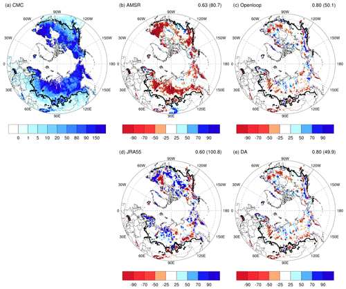
Figure 3 (a) Climatology of SWE (unit: kg m⁻² or mm) from CMC used as a reference and (b–e) the differences from CMC for AMSR2, the baseline model simulation (Openloop), JRA-55, and the data assimilation (DA) results for April during 2013–2020. The black line represents the boundary of the transition region, defined as the climatological mean SWE of less than 16 mm. Each value on the top right is the pattern correlation with CMC for 26 482 pixels over 40° N and the root mean square difference (unit: kg m⁻² or mm) from CMC (parenthesis) for 15 323 pixels over 40–60° N. Negative values (areas) in red shades are indicated with hatching.

Next, we compare the temporal variation of SWE as measured by the Spearman rank correlation coefficient with CMC, which is regarded as more appropriate than the Pearson correlation coefficient for describing datasets containing nonlinearity and outliers such as snow in both time and space. Figure 4 compares the distribution of correlation skills from AMSR2, Openloop, JRA-55, and DA. Openloop has a high performance in regions with heavy snow accumulation but relatively low performance in transition regions with significant snow changes. In contrast, the results from the AMSR2 satellite data represent poor performance in high-latitude areas with heavy snow accumulation but high performance in transitional regions, consistent with the previous studies (Gan et al., 2021). DA shows high performance not only in high-latitude areas with heavy snow accumulation but also in transition regions. Even compared to JRA-55 used as the atmospheric forcing, DA performs better in temporal variation. The quantitative results for the correlation in the Northern Hemisphere over 40° N (the transition region) are 0.41 (0.54) for AMSR2, 0.61 (0.48) for Openloop, 0.58 (0.58) for JRA-55, and 0.67 (0.61) for DA, respectively. The findings indicate that satellite retrievals offer additional value in capturing temporal variations through data assimilation, indicating the benefit of assimilating the AMSR2 SWE despite the overall lower performance of the satellite data itself.

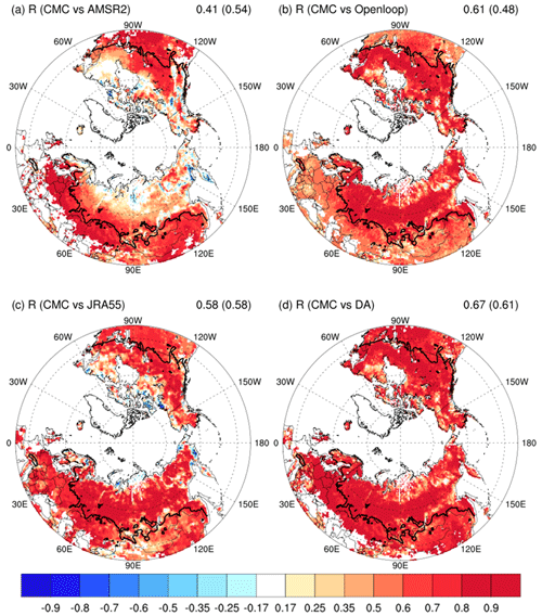
Figure 4 SWE skill measured as the Spearman rank correlation (R) with the CMC for AMSR2, baseline model simulation (Openloop), JRA-55, and the data assimilation (DA) result. The black line represents the boundary of the transition region, defined as the climatological mean SWE of less than 16 mm. Each value on the top is the area-average R of the Northern Hemisphere for 26 482 pixels over 40° N and for 8801 pixels over the transition region (parenthesis). Negative values (areas) in red shades are indicated with hatching.

The performance improvement by DA is also evident in the zonally averaged correlation coefficient shown in Fig. 5. The AMSR2 satellite data show higher performance than Openloop in the transition region around latitude 45–55° N, although performance sharply decreases with increasing snow accumulation. Openloop indicates gradually increasing performance as the latitude increases, with the highest performance at around 60° N. DA has a higher performance across the Northern Hemisphere, especially in the midlatitude transition region, than AMSR2 or JRA-55. An exception is for 35–40° N in the Tibetan Plateau, where JRA-55 used in situ observations. The results suggest that the developed snow data assimilation system represents not only the transitional regions but also the regions with high snow accumulation that are difficult to detect by satellite.

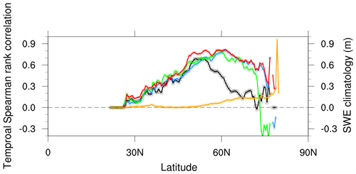
Figure 5 Zonally averaged Spearman rank correlation (R) along latitude for SWE. The yellow line indicates the climatology of SWE, and the black, blue, green, and red lines denote the values of AMSR2, baseline model simulation (Openloop), JRA-55, and data assimilation (DA) results, respectively.

Figure 6 presents the Spearman rank correlation depending on the SWE amount in the Northern Hemisphere. AMSR2 exhibits higher performance than Openloop for SWE up to 16 mm. However, the performance of AMSR2 sharply declines beyond that threshold, and Openloop shows a better performance. Consistent with the results illustrated in Figs. 4 and 5, DA demonstrates superior performance compared to others. Note that DA performs significantly better in the transition region with less than 16 mm of SWE. Considering that the area with less than 16 mm of SWE accounts for approximately 53 % of the entire area of the Northern Hemisphere (as shown in the pie chart in Fig. 6), the data assimilation impact is identifiable, and it can contribute substantially to the increase in the prediction skill by improving the simulation of the albedo changes and surface energy balance.

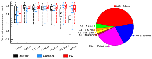
Figure 6 Box plots of the Spearman rank correlation (R) according to SWE (unit: kg m⁻² or mm). The pie chart shows the total area ratio (%) as a function of SWE amount. The black, blue, and red boxes denote the AMSR2, baseline model simulation (Openloop), and data assimilation (DA) results, respectively. The boxes indicate the 25 % and 75 % percentiles, and the line and point in the boxes show the median and the mean values. The upper and lower whiskers denote the 10 % and 90 % percentiles, respectively.

Consistent with the description in Sect. 3.3, this study considers an algorithm based on the highly reliable IMS satellite SCF data to identify the presence of snow and determine the assimilation process. Therefore, a further sensitivity test is conducted to investigate the influence of incorporating IMS data in snow assimilation. Figure 7 compares the correlation differences between Openloop and the data assimilation result employing both AMSR2 and IMS (DA), as well as the data assimilation result utilizing solely AMSR2 and excluding IMS (hereafter referred to as DA_AMSR2). The results obtained from the snow assimilation show improvements in the transitional regions where AMSR2 has better agreement with the observations compared to Openloop. Notably, the skill is enhanced significantly in DA by incorporating the IMS SCF. DA exhibits inferior performance compared to Openloop in certain exceptional cases, which may be attributed to discrepancies in snow identification between the CMC observations used for correlation and the IMS data utilized for data assimilation. Moreover, the performance of SWE improves even when only AMSR2 is used, but incorporating IMS leads to a substantial improvement in the transitional regions. This implies that IMS has a positive influence on the snow data assimilation.

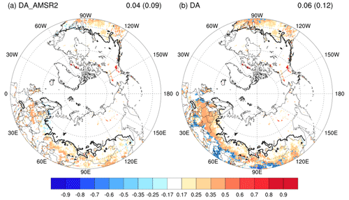
Figure 7 The difference in SWE Spearman rank correlation coefficient with CMC between the Openloop and data assimilation results: DA employing both AMSR2 and IMS and DA_AMSR2 utilizing solely AMSR2 and excluding IMS for April during 2013–2020. The black line represents the boundary of the transition region, defined as the climatological mean SWE of less than 16 mm. Each value on the top right is the area average over 40° N and the transition region (parenthesis). Negative values (areas) in red shades are indicated with hatching.

4.2 Kalman gain analysis

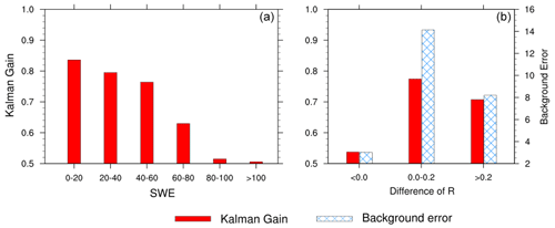
In order to better understand the skill enhancement through snow assimilation of satellite data, this section examines the Kalman gain. Figure 8 illustrates the spatial distribution of observation error, model background error, and the Kalman gain for SWE. A high value of the Kalman gain denotes that the assimilated result is closer to the AMSR2 observation than the model background. The Kalman gain is large when the background error becomes large, or the observation error is small. As this study specifies the observation error as a conservative 10 % of SWE compared to the previous study (Lee et al., 2015), the observation error basically follows a distribution similar to the climatological mean values. The background errors, originating from the 24 ensemble members, have higher values in high-latitude regions and midlatitude regions. Data assimilation methods such as LETKF used in this study often face challenges in accurately representing background errors when the ensemble spread is insufficient. Generally, the magnitude of ensemble spread is frequently compared to the root mean square error (RMSE). The ensemble spread in this study demonstrates a sufficiently valid magnitude in comparison with the RMSE, as illustrated in Fig. S1, indicating that it is well estimated. Moreover, the standardized distribution of SWE among the ensemble members exhibits a quasi-Gaussian distribution centered around zero, with the transition region showing a closer resemblance to a standardized Gaussian distribution (Fig. S4). In the spatial distribution of Kalman gain in Fig. 8c, significant performance improvement is observed in transition regions, where Kalman gains exhibit larger values. However, in high-latitude areas with substantial snow accumulation, there is a tendency for Kalman gain to have lower values. These findings agree well with the bar graph in Fig. 9, which illustrates the Kalman gain as a function of SWE amount. In the region encompassing the transition region with SWE amounts below 20 mm, the Kalman gain displays the highest values, particularly exceeding 0.8. As the SWE amount increases, the Kalman gain decreases, with a significant decline observed when the SWE amount reaches 80–100 mm or higher. Furthermore, in the areas where DA shows improved skill compared to Openloop, the Kalman gain shows values generally above 0.7. In contrast, relatively lower values below 0.5 are observed in the areas with decreased skill. This indicates that in the dominant areas of performance improvement, including the transition region, the background error is significantly larger than the observation error, emphasizing the substantial influence of observations in data assimilation. It is found that accurate remote sensing retrievals are well reflected in regions with high uncertainty in the LSM through the snow data assimilation system, leading to performance improvement.

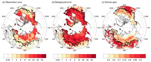
Figure 8 Spatial distribution of observation error (unit: kg m⁻² or mm), background error (unit: kg m⁻² or mm), and Kalman gain. The black line represents the boundary of the transition region, defined as the climatological mean SWE of less than 16 mm.

Figure 9 Bar chart of (a) the Kalman gain according to the SWE amount (unit: kg m⁻² or mm) and (b) the Kalman gain (red line) and background error (blue hatched line) as a function of the difference between Openloop and DA in the Spearman rank correlation coefficient (R).

4.3 Validation of the SWE for the extreme event

In April 2020, Siberia experienced a record-breaking heatwave with the highest observed average temperature. This section investigates the potential benefits of snow assimilation using satellite data for the case of the 2020 Siberian heatwave. Previous studies have identified a strong polar vortex accompanied by AO amplification during winter as a major cause of cold in the Eurasian region (Overland and Wang, 2021). Additionally, the occurrence of high temperatures in the Siberian region is found to be closely associated with large-scale atmospheric waves in the upper atmosphere over the Eurasian region originating from the Atlantic (De Angelis et al., 2023). As a result, remarkable snow melting occurred due to the high surface temperature over the Siberian region in April 2020, leading to extremely low values of SWE and SCF as depicted in Fig. S2. This is consistent with previous studies reporting significant snow depletion in 2020 in the region (Gloege et al., 2022). As shown in Fig. 10, significant negative anomalies in SWE and SCF are predominant over the transition region. Substantial snowmelt can contribute to record-breaking heatwaves through albedo feedback and changes in the ratio of the latent and sensible heat fluxes from the exposed surface, coupled with favorable atmospheric circulation patterns (Collow et al., 2022). Collow et al. (2022) demonstrated that the exposed surface contributed to up to 20 % of the temperature anomaly over Siberia in spring 2020. This implies the importance of realistic snow initial states in global coupled model forecasts. For the Siberian region with extreme high-temperature events marked by the red box in Fig. 10, DA shows better agreement with the extremely dry snow conditions, especially in the transitional region, compared to Openloop. These results are evident when considering the observation-to-model ratio in that region. The percentage of CMC (IMS) is 83 % (78 %) for Openloop and 93 % (89 %) for DA, indicating that DA with snow data assimilation based on satellite data effectively replicates the observed snow depletion in comparison with Openloop. Similarly to the 2020 case, we obtained another significant case in 2014 compared to Openloop, as shown in Fig. S3. Such extremely dry snow conditions can contribute to significant heatwave events in the following months.

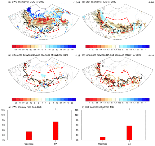
Figure 10 Anomalies of (a) SWE (unit: kg m⁻² or mm) from CMC and (b) SCF from IMS as well as the difference (c, d) of variables between DA and Openloop in April 2020. The bar chart (e, f) indicates the ratio of DA and Openloop to verification data such as CMC and IMS in the red box (48–65° N and 55–120°E), which is the region associated with extreme high-temperature events focused on this study. Negative values (areas) in red shades are indicated with hatching.

5 Conclusions and discussion

An advanced SWE data assimilation is developed in this study with the LETKF data assimilation method and the JULES LSM. The system assimilates snow water equivalent retrievals from AMSR2 and IMS snow cover. This constitutes an objective way to optimally combine two imperfect data sources for SWE from satellite remote sensing data and the land surface model simulation forced by observed atmospheric data. This study shows that the satellite-derived SWE has limitations in penetrating deep snow and exhibited high discrepancy from the SWE obtained from the Openloop LSM simulations. The SWE assimilation in this study proves the beneficial impacts of using satellite snow data, maintaining better analysis quality by dynamically balancing the errors from satellite observations and the model background states.

It is found that the simulation from Openloop as a baseline shows superior performance in high-latitude regions with heavy snow accumulation but relatively inferior performance in transition regions with much variation of snow in space and time. Contrastingly, the AMSR2 satellite data represent poor performance in high-latitude regions but exhibit relatively better performance in the transition regions. The SWE from the LETKF data assimilation consistently exhibits better performance in capturing the climatology and temporal variation compared to other results. It specifically improves the analysis in the midlatitude transition regions that cover approximately 53 % of the entire area of the Northern Hemisphere. It is found that the model background errors estimated from the ensemble spread are significantly larger than the observation errors, thereby reflecting satellite information more in those regions. The LETKF data assimilation also proves to be a reliable representation in the heavy snow regions due to low ensemble spread and large uncertainty in the satellite retrievals. Moreover, during the record-breaking heatwave in Siberia in April 2020, the remarkable snow depletion observed due to high surface temperatures is more realistically reproduced by our snow analysis compared to t Openloop.

This snow data assimilation framework is anticipated to contribute to a more precise prediction of atmospheric conditions by realistically capturing the interaction between the atmosphere and land, given the substantial influence of SWE on the energy and water balance at the interface of the atmosphere and land. Specifically, this applies to the transitional regions with high spatial and temporal variability. The long-term analysis of snow manifests a pronounced variability in the continental interior at interannual timescales, potentially improving the prediction of extreme heatwave events by global climate models. This study used the gridded CMC data from in situ observations for the validation. Although existing snow data are subject to uncertainty and limitations, we expect to obtain comparable conclusions and significant benefits by optimally combining satellite SWE data and the LSM simulations through the LETKF data assimilation method.

The quality of observations is crucial in a data assimilation system. Satellite-derived snow cover exhibits significantly higher accuracy compared to other data sources, while SWE has restricted performance due to the limitations of penetration depth by satellite sensors and relies heavily on estimation algorithms. Due to these problems, most previous studies and operational centers primarily depend on satellite-derived snow cover for snow initialization. However, the findings from this study highlighted the beneficial impacts of using satellite-derived SWE, particularly in the rapidly changing transition areas, to find out which variable is more important in closing surface energy and water balance changed by snow. Nevertheless, areas of significance in large-scale circulation, such as the Tibetan region, which experiences significant uncertainty and degraded performance in satellite data, do not exhibit substantial data assimilation effects. As the performance of SWE derived from various satellites continues to advance, these issues will be discussed more.