the Creative Commons Attribution 4.0 License.
the Creative Commons Attribution 4.0 License.
 | 30 Jan 2024
Modeling collision–coalescence in particle microphysics: numerical convergence of mean and variance of precipitation in cloud simulations using the University of Warsaw Lagrangian Cloud Model (UWLCM) 2.1
Piotr Zmijewski
Hanna Pawlowska
Numerical convergence of the collision–coalescence algorithm used in Lagrangian particle-based microphysics is studied in 2D simulations of an isolated cumulus congestus (CC) and in box and multi-box simulations of collision–coalescence. Parameters studied are the time step for coalescence and the number of super-droplets (SDs) per cell. A time step of 0.1 s gives converged droplet size distribution (DSD) in box simulations and converged mean precipitation in CC. Variances of the DSD and of precipitation are not sensitive to the time step. In box simulations, mean DSD converges for 103 SDs per cell, but variance of the DSD does not converge as it decreases with an increasing number of SDs. Fewer SDs per cell are required for convergence of the mean DSD in multi-box simulations, probably thanks to mixing of SDs between cells. In CC simulations, more SDs are needed for convergence than in box or multi-box simulations. Mean precipitation converges for 5×10³ SDs, but only in a strongly precipitating cloud. In cases with little precipitation, mean precipitation does not converge even for 105 SDs per cell. Variance in precipitation between independent CC runs is more sensitive to the resolved flow field than to the stochasticity in collision–coalescence of SDs, even when using as few as 50 SDs per cell.
- Article
(5799 KB) - Full-text XML
-
Supplement
(687 KB) - BibTeX
- EndNote


Particle microphysics (also known as Lagrangian particle-based microphysics, Lagrangian cloud models, or super-droplet microphysics) is a class of Lagrangian methods for numerical modeling of cloud microphysics that has been developed in the last decade (Shima et al., 2009; Andrejczuk et al., 2010; Sölch and Kärcher, 2010; Riechelmann et al., 2012). In particle microphysics, numerical objects called super-droplets (also known as simulational particles) are used as proxies for hydrometeors. Similarly to the more common Eulerian bin models, particle models explicitly resolve evolution of the DSD. There are several advantages of particle models that make them a compelling alternative to bin models (Grabowski, 2020): lack of numerical diffusion, easy modeling of multiple hydrometeor attributes (e.g., chemical composition), and scaling down to direct numerical simulations, among others. However, modeling of collision–coalescence has proven to be difficult in particle microphysics. A few algorithms have been developed to do this; see Unterstrasser et al. (2017) for a review. Of these, the all-or-nothing (AON) algorithm from the super-droplet method (SDM) of Shima et al. (2009) was shown to give the most accurate DSD in box simulations (Unterstrasser et al., 2017) and has been widely adopted (Hoffmann and Feingold, 2021; Dziekan et al., 2021; Unterstrasser et al., 2020; Arabas and Shima, 2013; Shima et al., 2020).
A recent study has found discrepancies in rain production between different particle models that use AON, although the models agree well in modeling condensational growth (Hill et al., 2023). This shows that a better understanding of numerical convergence of AON is necessary before particle models can become the benchmark for microphysics modeling. Several studies have shown that AON is sensitive to the number of SDs, to the numerical time step, and to the way SDs are initialized (Shima et al., 2009; Unterstrasser et al., 2017; Dziekan and Pawlowska, 2017; Schwenkel et al., 2018; Dziekan et al., 2019; Unterstrasser et al., 2020). Detailed studies of numerical convergence of AON have so far been done only in simulations of pure collision–coalescence in a box (Unterstrasser et al., 2017) and in a 1D column (Unterstrasser et al., 2020). It was found that criteria for convergence of AON are different in 1D than in box simulations. This shows that to confidently model precipitation in large eddy simulations (LESs) with particle microphysics, it is not sufficient to use parameters that give convergence in a box or a 1D column. The aim of this study is to better understand numerical convergence of AON in LESs.
We begin with a study of numerical convergence of AON in simulations of collision–coalescence in a box model. Although a similar study was done by Unterstrasser et al. (2017), we believe that it is valuable to repeat it for a number of reasons. Firstly, our implementation of particle microphysics differs in the details from that of Unterstrasser et al. (2017), so it may converge differently. Understanding convergence of our implementation in a box model is useful for planning convergence tests in more realistic simulations done afterward. Secondly, we compare with one-to-one simulation (Dziekan and Pawlowska, 2017), which is a more detailed reference model than was used in Unterstrasser et al. (2017). This allows us to study convergence not only of the mean DSD, but also of the variance of the DSD. Lastly, we validate results of Unterstrasser et al. (2017).
Next, we study convergence of AON in multi-box simulations. This simulation type, introduced by Schwenkel et al. (2018), is similar to box simulations, but the domain is divided into multiple coalescence cells and super-droplets can move between these. In that way they are more similar to LESs than box simulations, and, unlike in LESs, reference solutions can be produced by one-to-one simulations. The goal of multi-box simulations is to study how mixing of super-droplets between cells affects the minimum number of super-droplets required for convergence.
Finally, we study numerical convergence of AON in 2D simulations of isolated cumulus congestus. It is a much more realistic simulation than was used before for convergence tests of AON. The same processes are included as in an LES, with the only difference being smaller dimensionality. The reason why we use 2D instead of 3D is that this decreases the required computational power and memory size, allowing us to study a broader range of parameters. AON is a stochastic algorithm, so it gives different realizations of collision–coalescence in independent simulation runs. LES runs often also differ due to random differences in initial conditions. These differences in initial conditions include random perturbations of thermodynamic variables (e.g., temperature and humidity) and random initialization of SD attributes. Stochasticity in AON, as well as in initial conditions, leads to differences in flow fields, which can strongly impact results. To isolate the effect of stochasticity of AON from stochasticity of initial conditions, we use the same initial conditions in ensembles of simulations. Moreover, to facilitate studying convergence of AON, we use the same flow field for different simulations. This way, flow field is not affected by different realizations of AON. We also perform reference “dynamic” simulations with differences in initial conditions and without a prescribed flow field. This allows us to assess the importance of stochasticity of AON relative to other sources of stochasticity in LESs.
We start with a presentation of the particle microphysics scheme, with emphasis on AON and on the SD initialization procedure (Sect. 2). Studies of numerical convergence of AON in box, multi-box, and 2D simulations are presented in Sects. 3, 4, and in 5, respectively. Conclusions for cloud modeling are discussed in Sect. 6.
In Lagrangian particle microphysics methods, particles in the air (aerosols, haze particles, cloud droplets, raindrops, ice particles) are represented by computational objects called super-droplets. In most cases, each SD represents numerous identical real particles. The number of real particles an SD represents is called its multiplicity ξ (also known as weighting factor). Another commonly used SD attribute is spatial position. Two additional attributes are useful for modeling warm microphysics: wet radius, which describes the total volume of a particle, and dry radius, which describes the volume of the dissolved matter. For most processes (advection, condensation, sedimentation), changes in SD attributes are described by the same equations that describe how single real particles are affected by these processes. However, it is not straightforward to model collision–coalescence of SDs. In the next two sections, we present parts of the microphysics model that are particularly important for modeling collision–coalescence.
2.1 Initialization of SD radii and multiplicities
Multiplicities and radii of SDs are initialized from a prescribed initial size distribution. In this section, we describe common methods for doing this. The prescribed radius can either be wet or dry radius. We denote the initial number of SDs per grid cell with .
In one initialization method, all SDs have the same multiplicities and their initial radii are drawn from the distribution using inverse sampling (Shima et al., 2009; Hoffmann et al., 2015). Multiplicity is equal to the initial number of droplets in a cell divided by . Following Unterstrasser et al. (2017), we refer to this method as ξconst-init.
Another method of initialization is to divide the initial distribution into bins of equal sizes on a logarithmic scale. We denote the number of bins with . Within each bin we randomly select the radius of a single SD, and its multiplicity follows from the initial distribution. It is not obvious what should be the choice of the leftmost and rightmost bin edges. Arabas et al. (2015) proposed selecting bin edges so that multiplicities of SDs in the outermost bins are at least 1 (see Dziekan and Pawlowska, 2017, for details of the algorithm). In this method, bin edges depend on the volume of grid cells and, more importantly, on . When is increased, the largest possible initial SD radius is decreased. To counter this, Dziekan and Pawlowska (2017) proposed initializing additional SDs using inverse sampling from part of the distribution to the right of the rightmost bin. Note that the number of these additional SDs is rather small. In all simulations presented in this paper, we have . Following Dziekan and Pawlowska (2017), we will refer to this method as “constant SD-init”.
Instead of using the algorithm for finding bin edges, one can simply prescribe them. We call this method “constant SD fixed-init”. In this method, no SDs are added to represent the part of the distribution to the right of the largest bin.
Unterstrasser et al. (2017) compared multiple methods of SD initialization and found that using bins to initialize radii (as in constant SD-init) is preferable because it requires the fewest SDs to correctly model collision–coalescence. In most of the simulations presented in this paper, we use the constant SD-init. In Sect. 5.6 we study sensitivity to SD initialization method.
2.2 Collision–coalescence of SDs: the AON algorithm
The AON algorithm, developed by Shima et al. (2009), is an algorithm for modeling collision–coalescence in Lagrangian particle microphysics. It is derived from the stochastic description of the collision–coalescence of particles (Gillespie, 1975). In this description, it is assumed that the probability of collision between a pair of particles is known. AON is designed to give the correct expected number of collisions and to keep the number of SDs constant. The drawback of AON is that it gives a variance in the number of collisions larger than the real variance (Shima et al., 2009). The probability that a pair of super-droplets i and j will collide during some time interval is
where Pij is the probability of collision between two real particles with identical attributes (e.g., wet radii) as SDs i and j. It is given by , where Kij is the coalescence kernel, Δt is the time interval, and ΔV is cell volume (Shima et al., 2009). Coalescence of SDs i and j is defined as coalescence of pairs of real particles, with each pair made of one particle represented by SD i and one particle represented by SD j. Probability of SD coalescence can be greater than 1, in particular for long time steps. This represents multiple coalescence of the SD pair (Shima et al., 2009). Multiple coalescence can be done only if the ratio of multiplicities of colliding SDs is sufficiently high. If it is not sufficiently high, then the number of coalescence events will be artificially decreased. Note that in ξconst-init it is not possible to have multiple coalescence between an SD pair because all multiplicities are equal. For this reason, in our ξconst-init simulations we adapt the time step for coalescence to maintain collision probability below 1. The constant SD-init method typically gives large differences between multiplicities of SDs. Thanks to that, multiple coalescence is usually possible, and we can use a constant time step for coalescence in this type of simulation.
In some implementations of AON, the number of super-droplet pairs tested for coalescence per time step is equal to , where NSD is the number of SDs in a coalescence cell (the coalescence cell is typically equivalent to an Eulerian grid cell, Dziekan and Pawlowska, 2017). This is known as quadratic sampling (Unterstrasser et al., 2017, 2020). However, the original AON method of Shima et al. (2009) uses a technique called linear sampling, which is designed to speed up the algorithm. In linear sampling, non-overlapping pairs of super-droplets are considered per time step. The notation ⌊x⌋ represents the largest integer less than or equal to x. To obtain the correct expected number of collisions in linear sampling, the probability of collision between a pair of SDs is increased to
Linear and quadratic sampling techniques were directly compared in Dziekan and Pawlowska (2017) and in Unterstrasser et al. (2020). Unterstrasser et al. (2020) showed that quadratic sampling converges for a longer time step than the linear sampling (Fig. 6b therein). Once converged, both techniques give the same mean and variance (Dziekan and Pawlowska, 2017; Unterstrasser et al., 2020). Typically, the number of collision pairs tested per unit of time is smaller in linear sampling than in quadratic sampling, despite the shorter time steps. Moreover, in linear sampling all collision pairs can be computed in parallel because they are non-overlapping. For these reasons, we use linear sampling in this work.
We model collision–coalescence of droplets in a well-mixed box. For simplicity, we use r to denote wet radius in this section, as the dry radius is not important for collision–coalescence. We analyze the mass density function m(ln r), which is such that m(ln r)dln r is the mass of droplets per unit volume in the size range from ln r to ln r+dln r. The initial distribution of r is exponential in volume with 15 µm mean wet radius and 142 cm−3 droplet concentration, which gives 2 g m−3 liquid water content. This distribution was used in Onishi et al. (2015) and in Dziekan and Pawlowska (2017). The box volume is around 0.45 m3 and it initially contains 64 million droplets. Simulations are run for 300 s. We use a gravitational coalescence kernel with collision efficiencies from Hall (1980) and from Davis (1972).
Three types of collision–coalescence models are compared: the AON algorithm, one-to-one simulations, and the stochastic coalescence equation (SCE). AON is discussed in Sect. 2. One-to-one simulations are particle simulations with ξ=1; i.e., each real droplet is explicitly modeled. We use ξconst-init and linear sampling in one-to-one simulations. One-to-one simulations produce a realization in agreement with the master equation (Dziekan and Pawlowska, 2017). As such, they are the most fundamental type of simulation used and are considered to produce reference results. SCE is an equation for time evolution of the average DSD. It is typically used to model collision–coalescence in bin models. Dziekan and Pawlowska (2017) showed that the SCE gives correct average results for droplet populations greater than 107, so it should be valid in the box simulation with 6.4×10⁷ droplets discussed in this paper. We solve SCE with the Bott (1997) flux method with bin scaling parameter and time step 0.1 s. These parameters were found to give converged results.
One-to-one and AON simulations are stochastic. We run an ensemble of one-to-one simulations and ensembles of AON simulations for different values of . From these, we calculate the ensemble mean of the mass density function 〈m〉 and the ensemble standard deviation of the mass density function σ(m). The ensemble size in one-to-one simulations is Ω=10. In AON simulations, it is for and for . The SCE is deterministic; therefore, it does not require a simulation ensemble and it does not explicitly model variance of the DSD. However, Gillespie (1975) estimated the variance of the number of droplets in a given size range to be equal to the number of droplets in this size range. We validate this estimate by comparing it with one-to-one results.
3.1 Results of box simulations
First, we check how numerical time step Δtcoal affects AON simulations with , which is the number of SDs typical for LESs. In Fig. 1, we show DSDs at the end of the simulation for different time step lengths. There are no differences in 〈m〉 between Δtcoal=0.1 s and Δtcoal=0.01 s. Using Δtcoal=1 s results in 〈m〉 that is too large for the largest droplets. Δtcoal=10 s gives yet larger 〈m〉 for the largest droplets and also a decrease in 〈m〉 for droplets with radii between 40 and 100 µm. Regarding fluctuations, we see that differences in σ(m) correspond to differences in 〈m〉; e.g., 〈m〉 that is too large for the largest droplets also gives σ(m) that is too large for the largest droplets (Fig. 1a and b for Δtcoal=10). From this test, we conclude that mean DSD converges for Δtcoal=0.1 s and that fluctuations in DSD are not sensitive to Δtcoal.
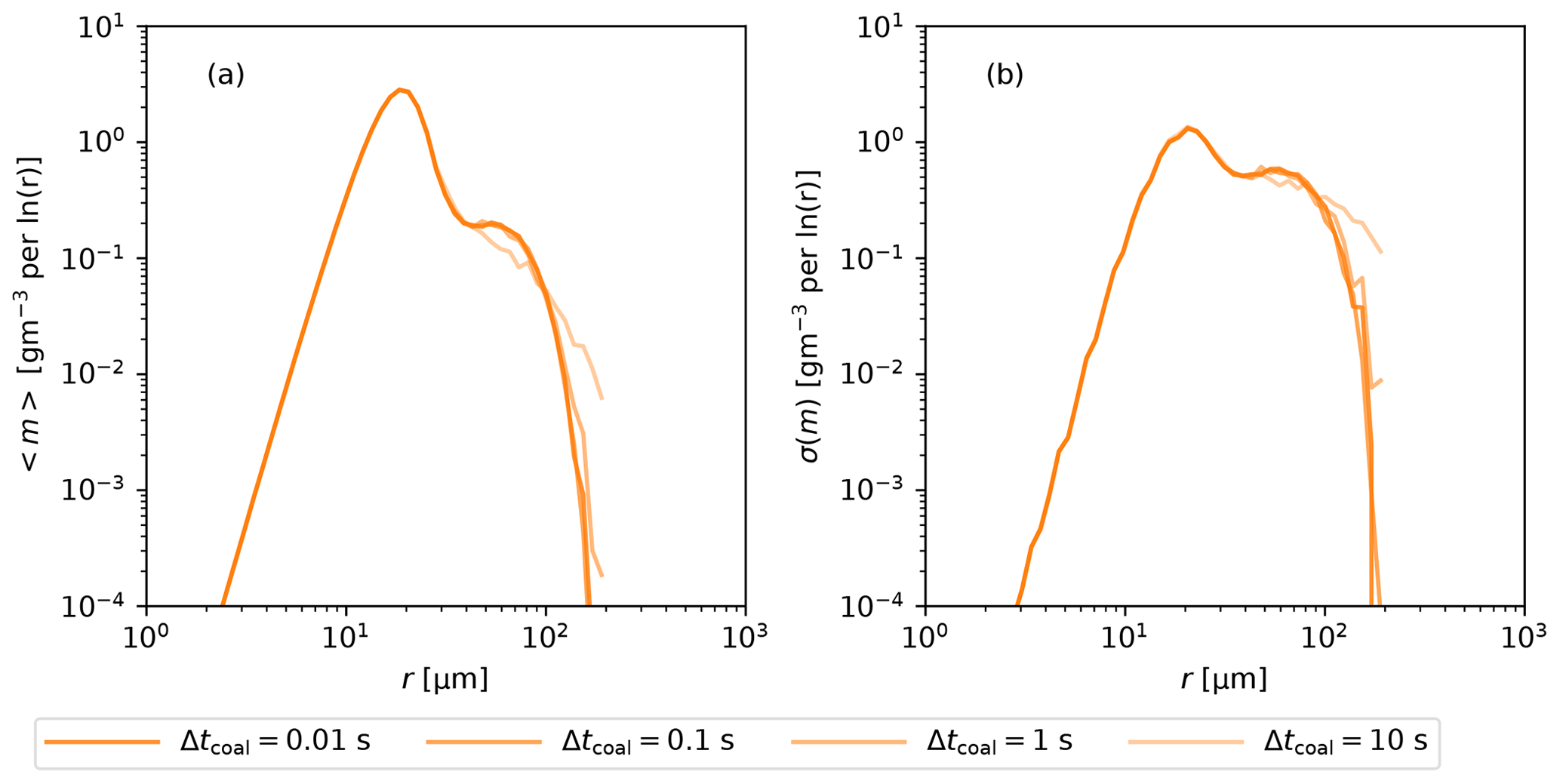
Figure 1(a) Mean and (b) standard deviation of the mass density function m for box simulations at t=300 s for different time step lengths.
Next we check how results are affected by the number of SDs for Δtcoal=0.1 s. In Fig. 2 we show DSDs at the beginning and at the end of an AON simulation for different . Results of one-to-one simulations and of the SCE are plotted for reference. The initial 〈m〉 is very well represented for all methods of radius initialization and agrees well with the SCE initialization (Fig. 2a). The first 11 moments of the initial distribution are plotted in the Supplement. The difference between moments from simulations and the expected moments is up to 11 % in AON and up to 3 % in SCE. The difference between moments in AON for various is negligible. Differences in initialization may cause differences between results of AON and SCE, but not between results of AON with different . The initial σ(m) decreases approximately linearly with increasing (Fig. 2b). gives smaller initial σ(m) than one-to-one, despite the much higher number of SDs in the latter (6.4×10⁷). The reason for this is the differences in the radius initialization procedure. The mean DSD at the end of the simulation does not significantly differ between different types of simulations, except for , which gives too few droplets with radii between 30 and 130 µm and too many droplets with r>130 µm (Fig. 2c). Fluctuations in DSD at the end of AON simulations decrease with increasing (Fig. 2d). We find that the standard deviation σ(m) is approximately proportional to , in particular for . Since multiplicity is inversely proportional to , the standard deviation is proportional to the square root of multiplicity, as estimated by Shima et al. (2009). Even for , σ(m) in AON is much larger than the reference one-to-one result. It is seen that σ(m) estimated from the SCE as the square root of the number of droplets, as proposed by Gillespie (1975), is larger than the one-to-one result but much closer to it than σ(m) in AON with .
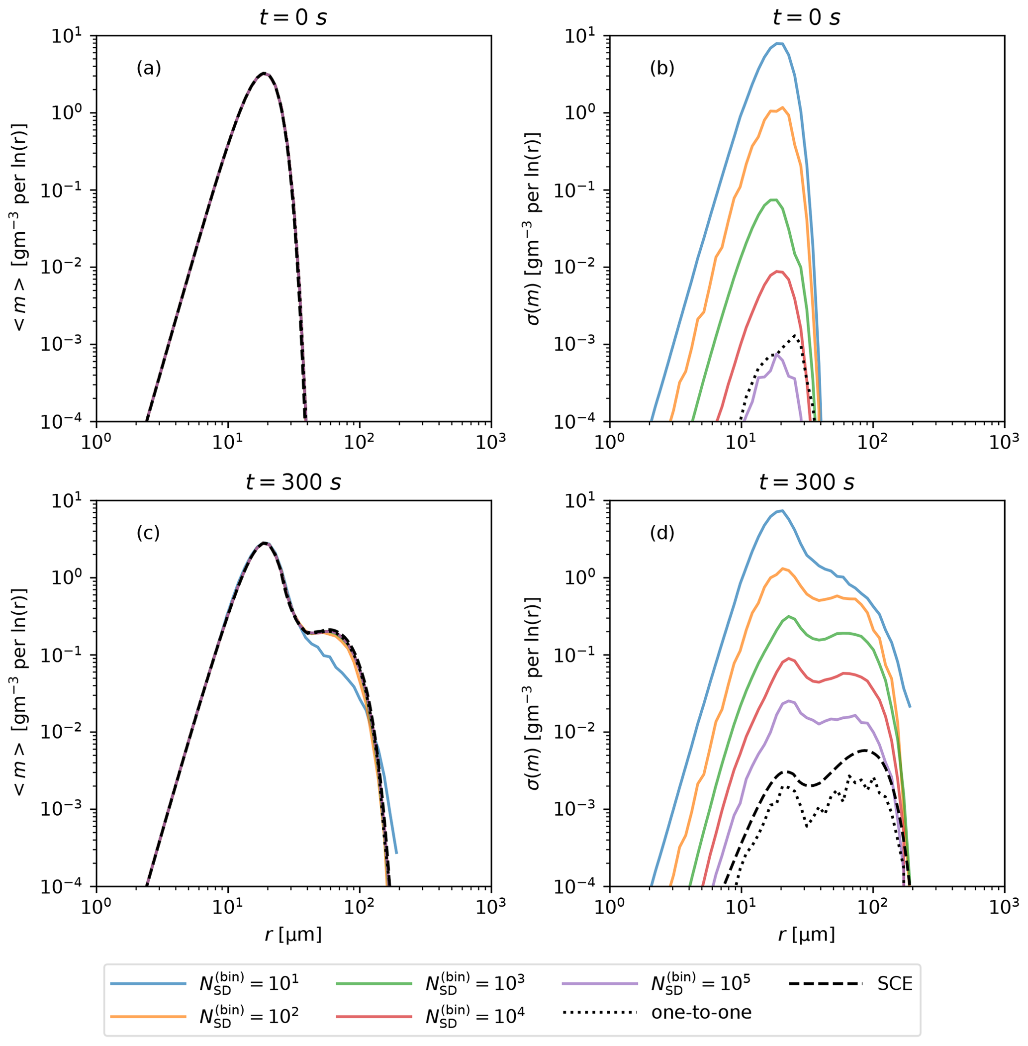
Figure 2Mean and standard deviation of the mass density function m from box simulations at t=0 s (a–b) and at t=300 s (c–d). Two types of Lagrangian simulations (SDM with Δtcoal=0.1 s and with various ; one-to-one simulations) and solutions to the SCE are compared.
Differences in 〈m〉 between simulations for different combinations of and of Δtcoal may potentially lead to differences in the mean amount of rain in LESs with Lagrangian particle microphysics. To have a better view of this issue, we plot differences between 〈m〉 in one-to-one simulations and 〈m〉 in AON simulations with different (Fig. 3). In the plot, 〈m〉 is multiplied by the terminal velocity to get the sedimentation mass flux of droplets of given size. This analysis confirms that results converge for Δtcoal=0.1 s, irrespective of (Fig. 3a–c). Longer time steps result in underestimation of the sedimentation flux for droplets with radii between around 40 and around 120 µm and in overestimation of sedimentation flux for other droplets. Regarding convergence with , we find that AON results agree with one-to-one for (Fig. 3d). For , the mass flux is overestimated for r<30 µm and r>130 µm and underestimated for 30 µm µm. Using underestimates mass flux for r>50 µm (Fig. 3d).
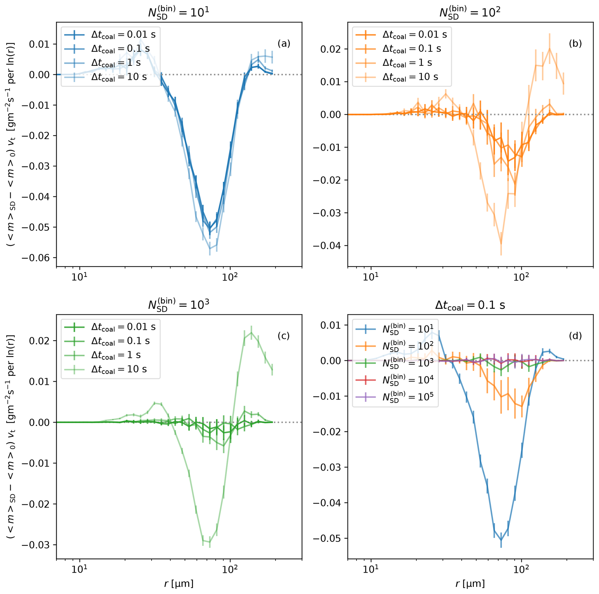
Figure 3Differences between 〈m〉 from SDM (〈m〉SD) and one-to-one (〈m〉0) Lagrangian microphysics, multiplied by terminal velocity vt. Results of box model simulations at t=300 s. Vertical error bars show the 95 % confidence interval.
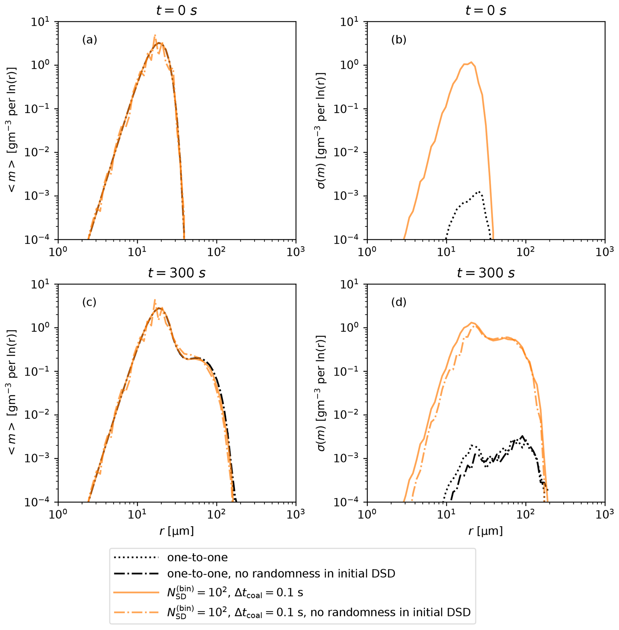
Initialization of droplet radii in Lagrangian particle microphysics is often stochastic (Shima et al., 2009; Unterstrasser et al., 2017; Dziekan and Pawlowska, 2017). It is a source of random differences between simulations that is separate from the stochastic collision–coalescence algorithm. We want to check how important these two different sources of randomness are for variance in the modeled DSD. We run ensembles of simulations that do not differ in the initial DSD but differ only in the realization of collision–coalescence. Comparison of these simulations with simulations that differ in both the initial DSD and the realization of collision–coalescence is shown in Fig. 4. The comparison is done for one-to-one simulations and for AON simulations with . The initial 〈m〉 agrees well for all types of simulations (Fig. 4a). As expected, the initial σ(m) is equal to zero for simulations without randomness in the initial DSD (Fig. 4b). At the end of the simulation, 〈m〉 agrees well between simulations with and without randomness in initial DSD (Fig. 4c). For droplets with r>20 µm, σ(m) at the end of the simulation is also not sensitive to randomness in the initial DSD (Fig. 4d). Lack of randomness in the initial DSD results in slightly smaller σ(m) for r<20 µm (Fig. 4d). Considering that collision–coalescence is responsible for formation of large droplets and that smaller droplets are formed by condensation, we conclude that the randomness in the initial DSD is not important for the mean or fluctuations in large droplet production.
3.2 Summary of box simulations and comparison with previous studies
Box simulations of collision–coalescence with AON show convergence of 〈m〉 for Δtcoal≤0.1 s, irrespective of , and for . The standard deviation σ(m) is not sensitive to Δtcoal but decreases with increasing . In one-to-one simulations, variance of the number of droplets in a size bin is approximately equal to the number of droplets in the bin, as predicted by Gillespie (1975). This relationship could be used to model the stochastic nature of collision–coalescence in bin microphysics.
Box model tests of the mean DSD in the AON algorithm were previously done by Shima et al. (2009) and Unterstrasser et al. (2017). Unterstrasser et al. (2020) did column simulations and some of them did not include sedimentation, which is equivalent to box simulations. Shima et al. (2009) found relatively good agreement with the SCE for Δtcoal=0.1 s and for . The time step requirement is the same as found in this work, but the required is much higher. The latter is probably because Shima et al. (2009) used the constant multiplicity initialization, which was found by Unterstrasser et al. (2017) to require many more SDs than their “singleSIP” initialization; this is similar to our constant SD initialization.
Using the singleSIP initialization, Unterstrasser et al. (2017) showed that results are close to converging for Δtcoal=1 s (Fig. 18 therein, first column). An important difference between this work and Unterstrasser et al. (2017) is that the latter used quadratic sampling. Differences between linear and quadratic sampling methods are discussed in Sect. 2.2. Regarding convergence with , Unterstrasser et al. (2017) found convergence for (Fig. 18 therein, second column; there κ=200 corresponds to ) and Unterstrasser et al. (2020) did not find convergence for up to (Fig. 6a therein). Convergence tests in Unterstrasser et al. (2017) and in Unterstrasser et al. (2020) were done by analyzing moments of the DSD, and it was most difficult to obtain convergence of the 0th moment (total droplet number). We find contrary results, i.e., that higher moments converge more slowly than lower moments. To illustrate this, we consider our box simulations for . In these simulations, Δtcoal=10 s gives a visibly different large end of the DSD than Δtcoal=0.1 s (Fig. 1). The 0th (total droplet number) and 2nd (radar reflectivity) moments are larger for Δtcoal=10 s than for Δtcoal=0.1 s by approximately 0.5 % and 30 %, respectively. This is consistent with the intuition that higher moments are more sensitive to the large end of the DSD, and it is the large end of the DSD that is most sensitive to collision–coalescence.
The AON implementation from the libcloudph++ library, which is used in this paper, was also used in box simulations described in Dziekan and Pawlowska (2017). That paper discussed convergence of t10 %, the time after which 10 % of cloud mass is turned into rain mass. Dziekan and Pawlowska (2017) found that for Δtcoal=1 s mean t10 % converges for (Fig. 4 therein). Dziekan and Pawlowska (2017) also showed that the standard deviation of t10 % decreases linearly with the square root of (Fig. 5 therein). This is in agreement with our observation that σ(m) is proportional to and with the theoretical prediction from Shima et al. (2009) (Sect. 4.1.4 therein).
The simulation setup is the same as in box simulations, but the domain is divided into C equal rectangular cells of volume m3. Only SDs that are in the same cell can collide with each other. Super-droplets move around the domain with a velocity that is a sum of the terminal velocity and of the air velocity, which is calculated from a synthetic isotropic turbulence model. Details of the turbulence model are given in Appendix A. Side walls are periodic. The turbulent kinetic energy dissipation rate is 10 cm2 s−3. Simulations are run for 300 s. The model time step is adapted to keep the Courant number in each direction smaller than 1 (but the time step is not longer than 0.1 s). The coalescence time step is equal to the model time step. When initializing SDs, the entire domain is treated as a single cell. Therefore, represents the total initial number of SDs (minus SDs from “tail” initialization). The mean number of SDs per cell at the start of the simulation is . Initial SD positions are selected randomly within the domain.
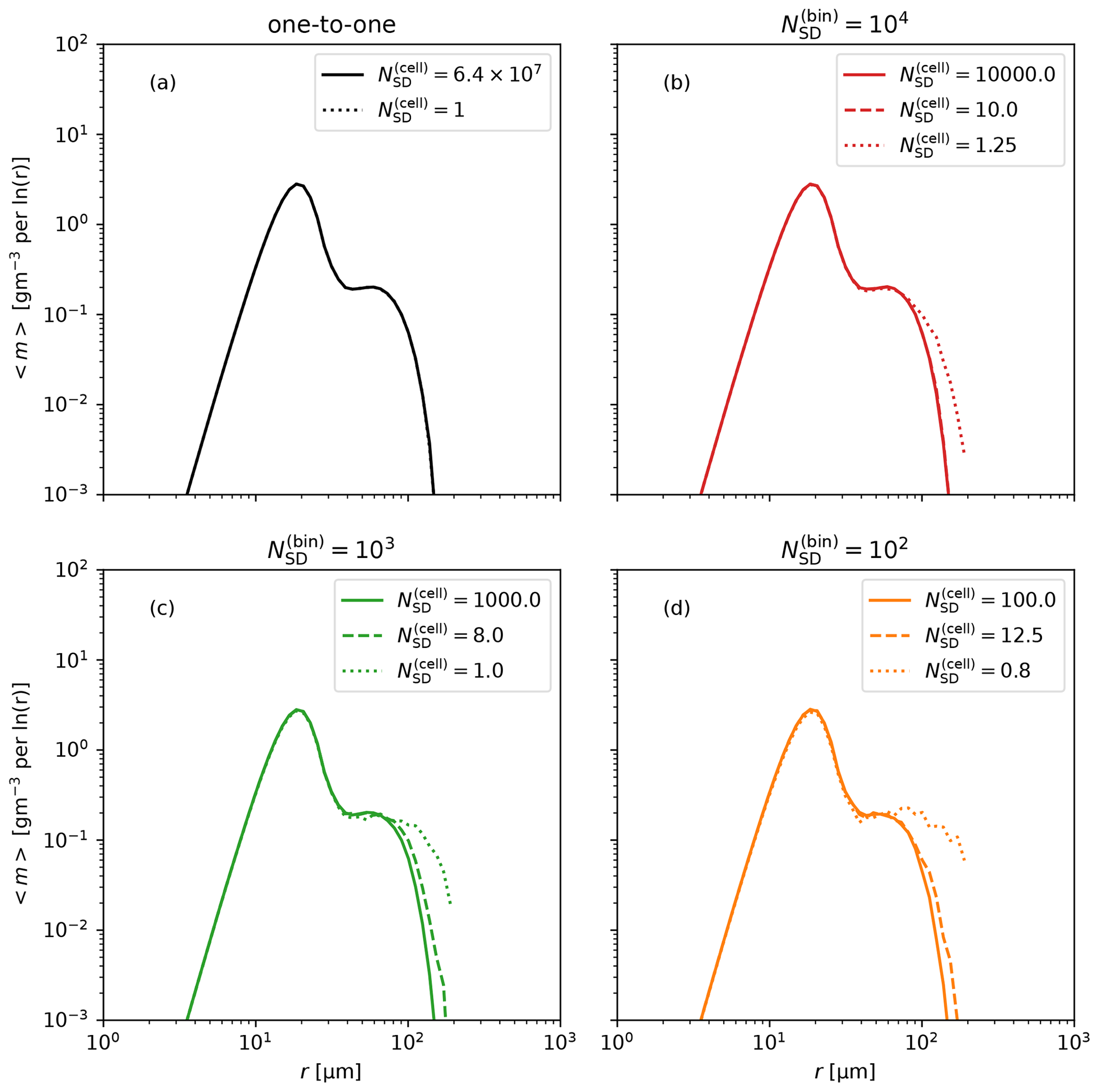
Figure 5Mean mass density function at the end of multi-box simulations from (a) one-to-one simulations and AON simulations with (b), (c), and (d). Each figure shows results for a differing number of cells, corresponding to differing .
We run ensembles of one-to-one and AON simulations for differing numbers of cells. The ensemble size is Ω=30 in one-to-one simulations and in AON simulations. The DSD at the end of the simulation is shown in Fig. 5. In principle, one-to-one simulations should become more realistic as the number of cells is increased ( is decreased). This is because droplet collisions are local; i.e., droplets need to get close together in order to collide. We find that in one-to-one simulations, there is no difference in results for and for (Fig. 5a). This shows that there is no error in assuming that the domain is well-mixed, i.e., that droplets are uniformly distributed within the domain. In AON simulations, each SD represents multiple droplets that are uniformly distributed within the cell in which the SD is located. As C is increased while is kept constant, all droplets represented by an SD are confined to a smaller volume. Therefore, increasing C leads to less uniform spatial distribution of droplet sizes. Results show that this can cause errors in the domain-averaged DSD (Fig. 5b–d). For large enough, box simulations (C=1, ) agree with one-to-one simulations (Fig. 3d). However, the same but with large C (small ) results in production of droplets that are too large (Fig. 5b–d). The minimal value of that gives correct results depends on can be smaller for larger (e.g., works well for , but gives errors for ). The number of coalescence cells does not affect σ(m) (not shown in the figure).
In line with the conclusions of Schwenkel et al. (2018) and Unterstrasser et al. (2020), multi-box simulations show that fewer SDs per cell are needed to correctly model collision–coalescence when mixing of SDs between cells is included. For example, box simulations with give significant errors, but multi-box simulations with and are close to the reference. It is important that the rate of intercell mixing decreases with increasing cell size, which affects the minimal required . Simulations for and give errors, while simulations for and give correct results. Cells are larger in the former case than in the latter case. Larger cells imply less intercell mixing and, in consequence, larger required for convergence.
In this section, we analyze AON in a two-dimensional simulation of an isolated cumulus congestus cloud. Conclusions about convergence of AON in box and multi-box simulations that were presented in the previous sections do not necessarily apply to higher-dimensional simulations or simulations that include more processes affecting the DSD (e.g., condensational growth). For example, Unterstrasser et al. (2020) found that it is easier to reach convergence in a one-dimensional column simulation than in a box simulation. Based on the fact that in box simulations 〈m〉 converges for large , we can expect that precipitation in the CC simulation also converges for large . However, it is possible that precipitation in CC is affected by the artificially large variance in AON, which is illustrated by the lack of convergence of σ(m) in box simulations. Variance in AON that is too large may result in differences in the DSD between cells that are too large. This might affect precipitation averaged over the entire cloud because there is mixing between cells. Variance that is too large may also cause differences in precipitation between independent simulation runs that are too large. However, it is possible that in cloud simulations spatial and temporal variability of DSD is more susceptible to other factors, e.g., changes in relative humidity. Then, variability in AON that is too large would not be a problem. Variance in the number of collisions is inversely proportional to (see Sect. 3). Doing CC simulations for different values of allows us to study how the artificially large variance in AON affects simulations, even though it is not possible to have large enough for the variance to converge. Box simulations suggest that the time step typically used in LESs is sufficient for convergence of AON, but we also do a time step convergence test in CC.
5.1 LES model and setup
The CC simulations are done with the University of Warsaw Lagrangian Cloud Model (UWLCM). UWLCM is an LES tool that allows 2D and 3D simulations with Lagrangian particle (or Eulerian bulk) microphysics. Thermodynamic variables (potential temperature, water vapor mixing ratio, velocity) are modeled in an Eulerian manner. The Lipps–Hemler anelastic approximation (Lipps and Hemler, 1982) is used to filter acoustic waves. For spatial discretization of Eulerian variables, the staggered Arakawa-C grid (Arakawa and Lamb, 1977) is used. The finite-difference method is used to solve equations for Eulerian variables. The multidimensional positive-definite advection transport algorithm (MPDATA) (Smolarkiewicz, 2006) is used to model transport of Eulerian variables. The model uses the generalized conjugate residual solver (Smolarkiewicz and Margolin, 2000) to solve the pressure disturbance. In this paper, subgrid-scale (SGS) transport of Eulerian variables is modeled using the implicit LES approach (Grinstein et al., 2007). Depending on the simulation type, SGS advection of SDs is either ignored or modeled as an Ornstein–Uhlenbeck (here denoted as OU) process that crudely represents homogeneous isotropic turbulence (Eq. 10 in Grabowski and Abade, 2017). A more detailed description of UWLCM can be found in Dziekan et al. (2019) and in Dziekan and Zmijewski (2022).
We use an isolated cumulus congestus modeling setup that was one of the cases studied at the International Cloud Modeling Workshop 2020. It is an adaptation of the setup developed by Lasher-Trapp et al. (2001). The computational domain is 12 km in the horizontal direction and 10 km in the vertical direction. Vertical profiles come from a conditionally unstable sounding from the Small Cumulus Microphysics Study field campaign. Initial potential temperature and water vapor mixing ratio fields are randomly perturbed below 1 km altitude. Perturbation amplitudes are 0.025 g kg−1 and 0.01 K. For the first hour, surface fluxes are uniform: 0.04 g kg−1 m s−1 latent heat flux and 0.1 K m s−1 sensible heat flux. Afterward, surface fluxes have a Gaussian distribution centered at the middle of the domain, with maxima 3 times larger than the uniform flux from the first hour and with half-width of 1.7 km. The momentum surface flux is given by a constant friction velocity 0.28 m s−1. The total simulation time is 3 h. The lateral boundaries are periodic, and the upper boundary is free-slip rigid-lid. We use an aerosol distribution based on observations from the RICO campaign (VanZanten et al., 2011). The distribution is made of two lognormal modes. The first-mode (second-mode) parameters are number concentration 90 cm−3 (15 cm−3), geometric mean radius 0.03 µm (0.14 µm), and geometric standard deviation 1.28 (1.75). Aerosol type is ammonium bisulfate. We model these relatively clean conditions in order to have a significant amount of precipitation, which is the focus of this study. A gravitational coalescence kernel is used, with collision efficiencies from Hall (1980) for large droplets and from Davis (1972) for small droplets. The coalescence efficiency is set to 1. There is no droplet breakup. Terminal velocities are calculated using a formula of Khvorostyanov and Curry (2002). The model time step is 0.5 s; the time step for condensation is 0.1 s and cell size is 100 m in each direction.
We use a 2D instead of 3D LES because it allows us to study much larger values of . The same processes are modeled in 2D as in 3D, e.g., condensation, advection, sedimentation, and collision–coalescence. In 2D, the modeled flow field has different characteristics than in 3D. We expect to see more variability between simulation runs in 2D than there would be in 3D because of a much smaller number of spatial cells. The rate of mixing of SDs between cells can also be different in 2D than in 3D. However, we think that the way this variability is affected by parameters of the microphysics scheme in 2D is representative of how it would be affected in 3D.
5.2 Simulation strategy
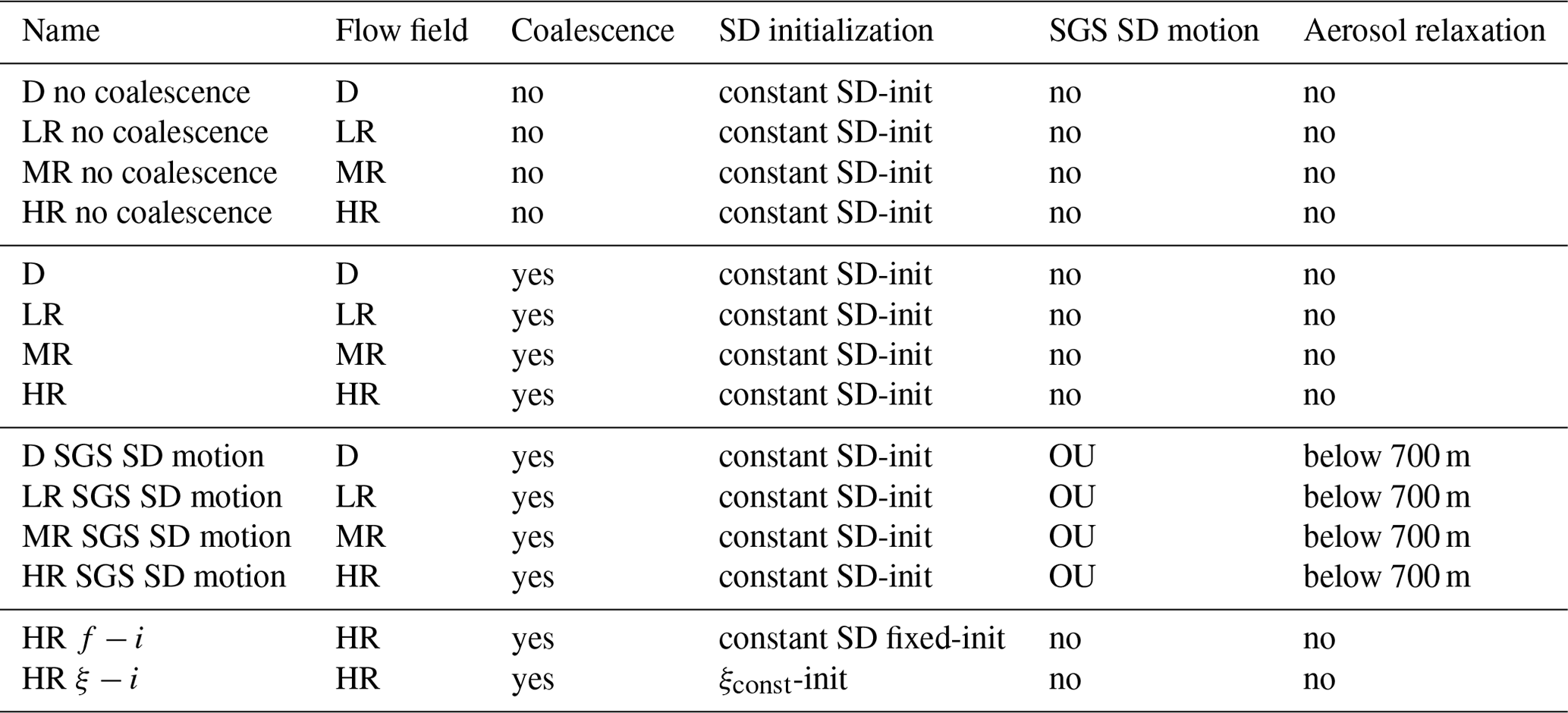
Typically, in LESs there is a random perturbation of initial conditions, e.g., of temperature and humidity. In LESs with particle microphysics, initial conditions may also differ in SD attributes because they are often randomly initialized. This randomness in initial conditions leads to differences in results between simulation runs, independently of AON. To understand the role of AON, we isolate its effect by comparing dynamic and kinematic simulations. In dynamic simulations, the pressure equation is solved, meaning that different realizations of microphysics lead to different flow fields. In kinematic simulations, the flow field is prescribed. Our strategy is to run an ensemble of dynamic simulations, denoted with D, with random differences in initial conditions. We consider this ensemble to be a control group because this is the way an LES is usually done. From dynamic simulations, we select three realizations: one with little rain, one with medium rain, and one with a high amount of rain (LR, MR, and HR, respectively). Flow fields from these simulations are used to run ensembles of kinematic simulations. In kinematic simulations, initial conditions do not change within an ensemble. Therefore, any variability within a kinematic ensemble is solely caused by AON. Our goal is to study convergence of precipitation, which is a variable sensitive to modeling collision–coalescence. We also study convergence in simulations without collision–coalescence to make sure that convergence in simulations with collision–coalescence is only related to AON. The number of simulations of each type is given in Table 2.
To generate velocity fields for kinematic simulations, we run numerous dynamic simulations. Our goal is to find three velocity fields that would give significantly different amounts of rain. In a single dynamic simulation, the amount of precipitation depends not only on the realized flow field, but also on the realization of the AON algorithm. This means that rain from a single dynamic simulation is not representative of the expected amount of rain from a series of simulations with the same velocity field. To be sure that we selected velocity fields that will give different amounts of rain, first we chose a candidate velocity fields based on the amount of rain in the single dynamic run, and then we ran 20 kinematic simulations and used the average from these 20 simulations as the expected amount of rain for a given velocity field. Note that these 20 simulations were just a preliminary ensemble to estimate the expected amount of precipitation and that the final number of simulations was much larger (it is given in Table 2). Based on this procedure, we selected the three velocity fields for kinematic simulations: LR, MR, and HR. The histogram of the distribution of accumulated surface precipitation in the dynamic simulation ensemble is shown in Fig. 6. These highlighted bins delineate the range of original precipitation values from the velocity fields that were considered.
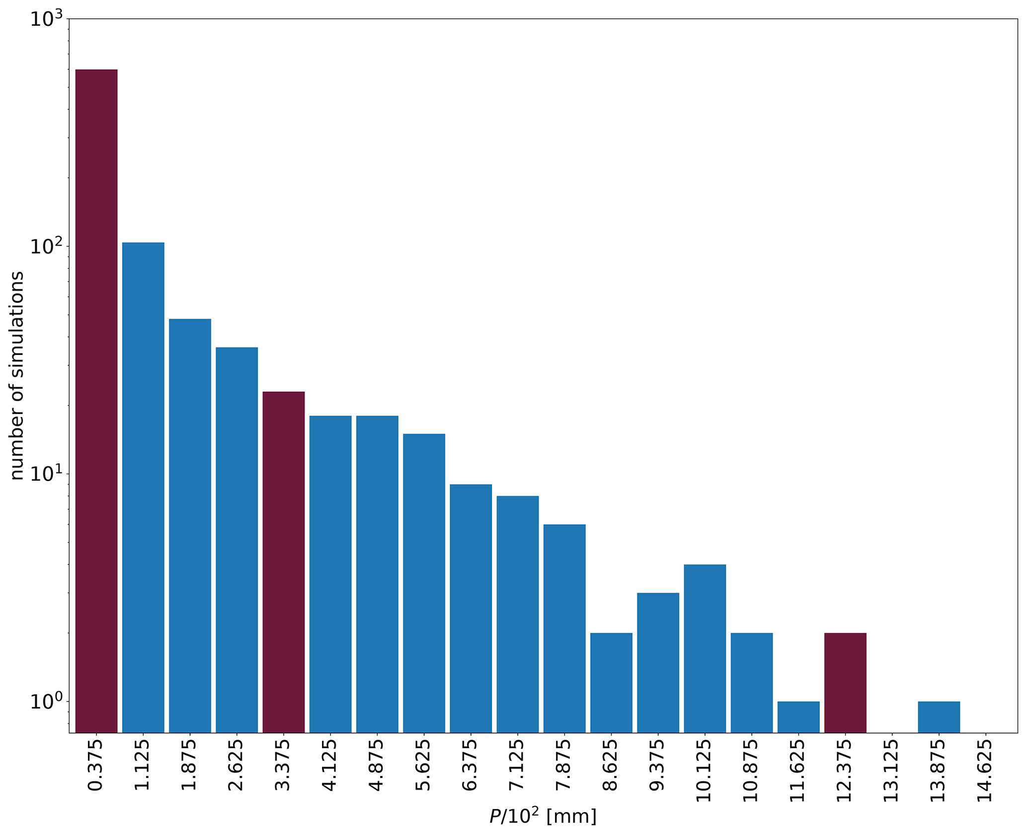
Figure 6Frequency histogram of accumulated surface precipitation (P) from the ensemble of dynamic simulations with . The horizontal axis is the bin center. Bin width is mm. The vertical axis is the number of simulations with P within a bin. The bins in burgundy show the expected rain amount for LR, MR, and HR velocity fields (left to right).
Besides using different flow fields, we study sensitivity to the model of SGS advection of SDs to the SD initialization method, and we run simulations without collision–coalescence. A list of all simulation types is given in Table 1.
Table 1Configuration of CC simulations. Columns, from left to right, show the configuration name, type of flow field (dynamic or kinematic), collision–coalescence on/off flag, the method for SD initialization, and the model of SGS advection and aerosol relaxation method (discussed in Sect. 5.7).
5.3 Temporal development of cloud
In this section we discuss time series of general cloud properties in the D, LR, MR, and HR scenarios (with collision–coalescence). This is done to give readers an idea about how the modeled cloud develops. Time series of cloud-top height (CTH), cloud cover (cc), cloud water path (CWP), rainwater path (RWP), and surface precipitation are plotted in Fig. 7. The results are ensemble averages. For brevity, only results for are shown. Time series for other values of are similar and are available in the Supplement.
Time series of CTH, cc, and CWP are smoother in dynamic than in kinematic simulations. In dynamic simulations, there are differences between simulation runs at the moment when the cloud starts to develop. When averaged over simulation runs, the results are smooth. In kinematic simulations, cloud develops in a very similar way in all simulations within an ensemble. Therefore, the ensemble average resembles a single dynamic simulation in that it changes significantly at short timescales. This illustrates that, unsurprisingly, CTH, cc, and CWP are more sensitive to the airflow than to the realization of collision–coalescence.
In all scenarios, cloud starts to develop at around 1500 s. Afterward, it deepens with time, reaching maximum cc at around 5500 s and maximum CWP between 7000 and 8000 s, depending on the case. In kinematic scenarios, rain appears shortly after CWP reaches its maximum. The cloud almost entirely disappears at around 9500 s (CWP close to 0). A second cloud starts to develop near the end of the simulation, indicated by an increase in CWP. The differences in rain between LR, MR, and HR are explained by differences in CWP, with highest CWP giving the most rain. In MR and in HR, CWP steadily increases until rain is formed. The difference is that CWP and CTH reach higher values in HR than in MR. In LR, there are multiple local maxima of CWP, each of them smaller than the maxima in MR and HR.
Table 2Simulation ensemble sizes for all simulation types (defined in Table 1) and all tested values of and Δtcoal.
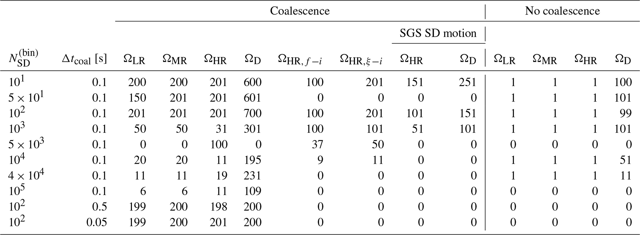
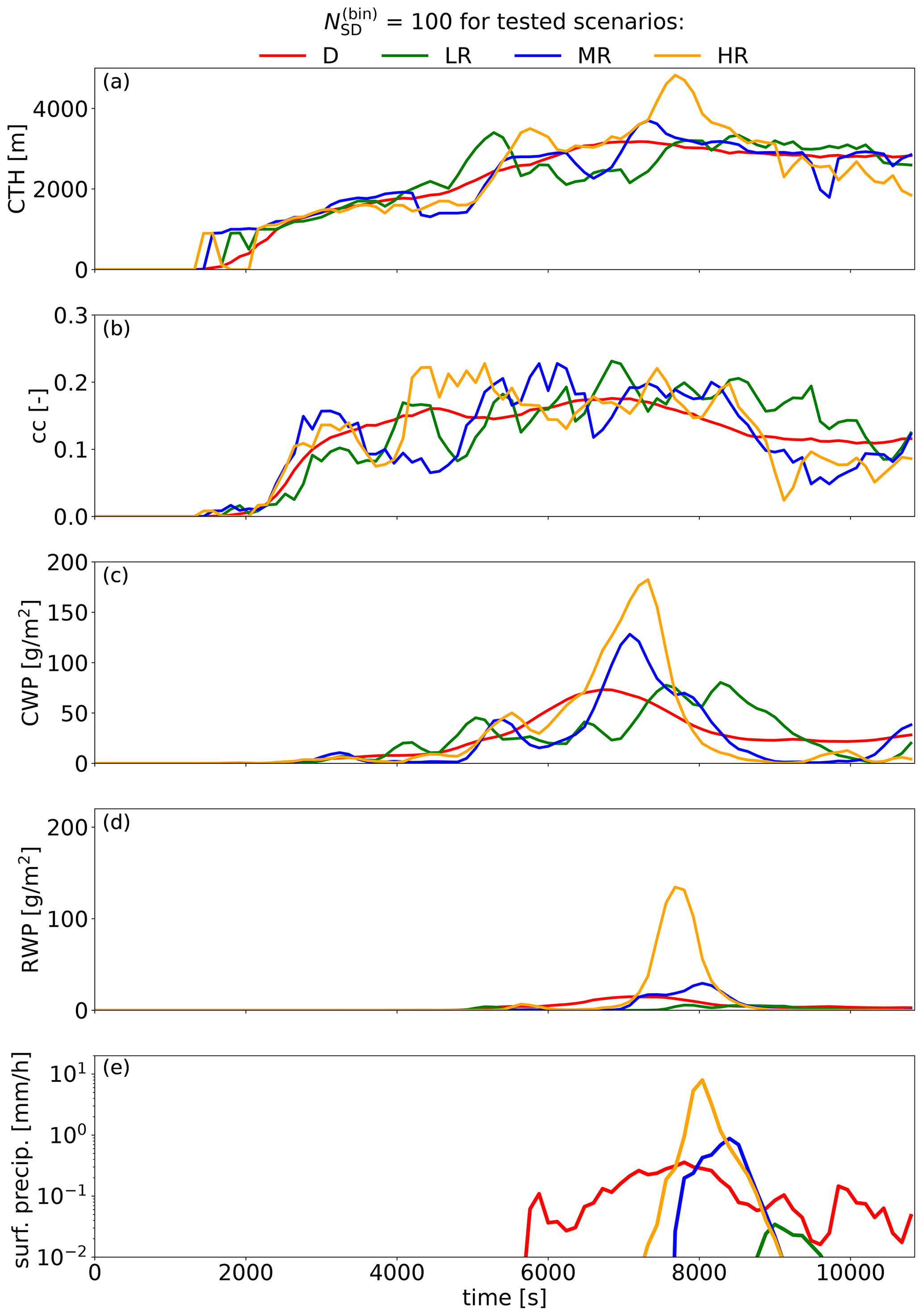
Figure 7Time series of ensemble averages of cloud-top height, cloud cover, cloud water path, rainwater path, and surface precipitation for D, LR, MR, and HR scenarios with . Cloud-top height (CTH) is the vertical position of the topmost cloudy cell. Cloud cover (cc) is the fraction of columns with at least one cloudy cell. Cloudy cells are cells with a cloud water mixing ratio greater than 10−5. Cloud droplets are droplets with 0.5 µm µm. Raindrops are droplets with 25 µm ≤rw. Surface precipitation (surf. precip.), cloud water path (CWP), and rainwater path (RWP) are domain averages divided by cc in order to obtain values representative of the cloudy area.
5.4 Numerical convergence in simulations without collision–coalescence
To reliably study convergence of the collision–coalescence algorithm, we first need to make sure that simulations without the collision–coalescence process have converged. The time step for condensation used in all simulations, 0.1 s, was found to give converged results (not shown). Here we focus on convergence with the number of SDs. Time series of basic cloud properties (cloud water content, cloud cover, and cloud-top height) agree for (they are plotted in the Supplement). Convergence of the DSD is analyzed by comparing profiles of concentration, mean radius and relative dispersion of the radius of cloud droplets (Fig. 8). Of the three parameters, relative dispersion is the slowest to converge as it requires .
Note that the relative dispersion around 0.2 is within the lower part of the range of values observed in cumuliform (Lu et al., 2013) and stratiform (Miles et al., 2000; Pawlowska et al., 2006) clouds. This indicates that the DSD is realistic, an important point because Lagrangian models tend to generate narrow DSD. A DSD that is too narrow would result in a rate of collision–coalescence that is too low, and for slow collision–coalescence it is more difficult to reach convergence (Dziekan and Pawlowska, 2017). Therefore, studying convergence for an unrealistically narrow DSD could give convergence requirements that are too strict.
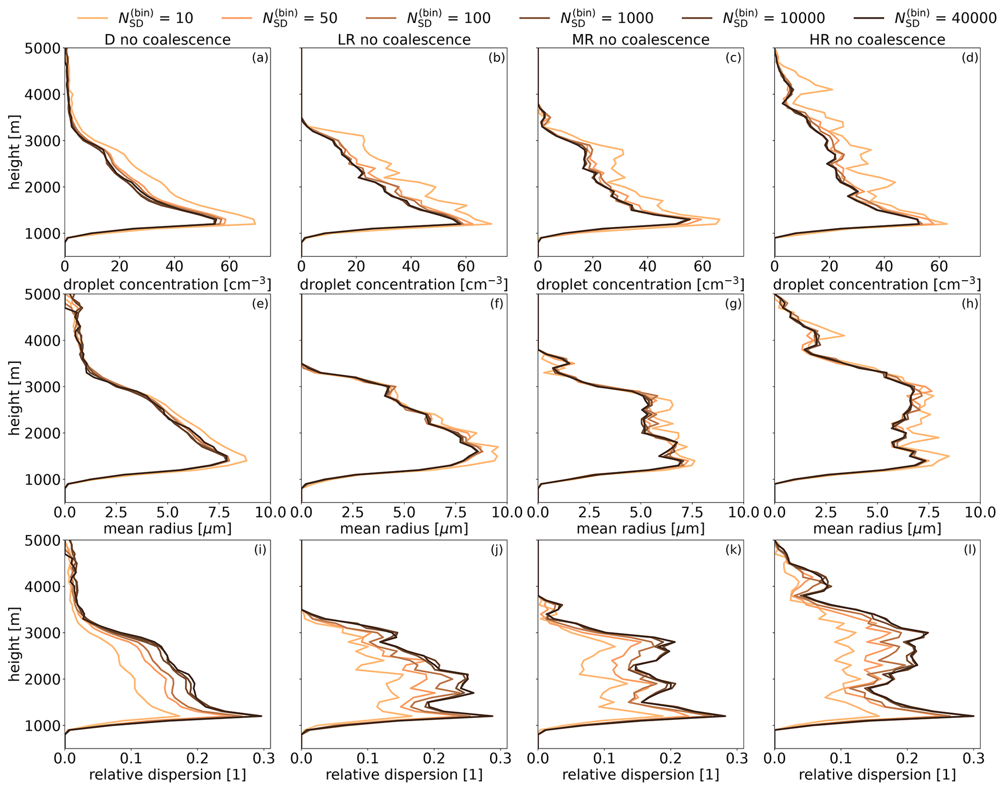
Figure 8Profiles of cloud droplet concentration (top row), cloud droplet mean radius (center row), and relative dispersion of cloud droplet radius (bottom row) from simulations without collision–coalescence. Profiles are averaged over cloudy cells, over the time interval between 1800 and 9600 s, and over the ensemble of simulations.
5.5 Numerical convergence of precipitation
From now on, only simulations with collision–coalescence will be discussed. Profiles of precipitation flux for different numbers of SDs are shown in Fig. 9. We find that if there are differences between these profiles, they are similar at all levels (with very few exceptions). For example, at all levels gives less precipitation than . This shows that convergence of precipitation at one level is representative of convergence in the entire cloud. Therefore, we choose to study surface precipitation in detail, in particular the accumulated surface precipitation P. We denote the ensemble mean with 〈P〉 and ensemble standard deviation with σ(P). For estimating errors of ensemble statistics, we use the following formulas. The standard error of 〈P〉 is
where n is ensemble size. The standard error of σ(P) is (Rao, 1973, p. 438)
The 95 % confidence interval of 〈P〉 is
The 95 % confidence interval of σ(P) is (Sheskin, 2011, p. 217)
where f(x, y) is the inverse CDF of the chi-squared distribution.
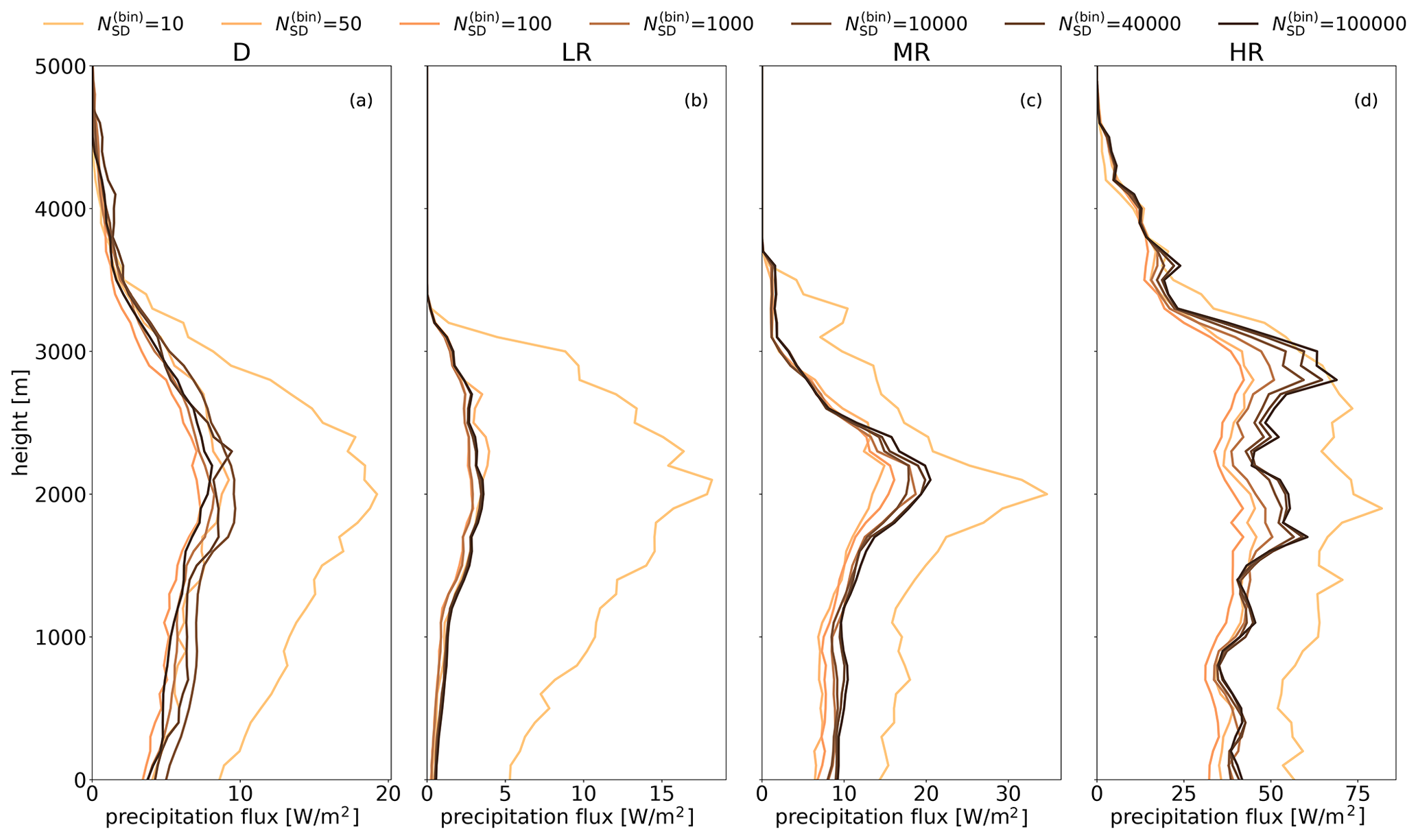
Figure 9Profiles of precipitation flux in simulations with collision–coalescence. Profiles are averaged over all cells, over the time interval between 1800 and 9600 s, and over the ensemble of simulations. Time step for coalescence is Δcoal=0.1 s.
Figure 10 shows the sensitivity of surface precipitation to Δtcoal, the time step with which coalescence is modeled. We find no statistically significant impact of Δtcoal on 〈P〉 or on σ(P) for Δtcoal≤0.5 s. Sensitivity to the time step was tested only for because box simulations showed that results converge for the same value of Δtcoal, independent of the value of . A study of the sensitivity to that is discussed next was done for Δcoal=0.1 s.
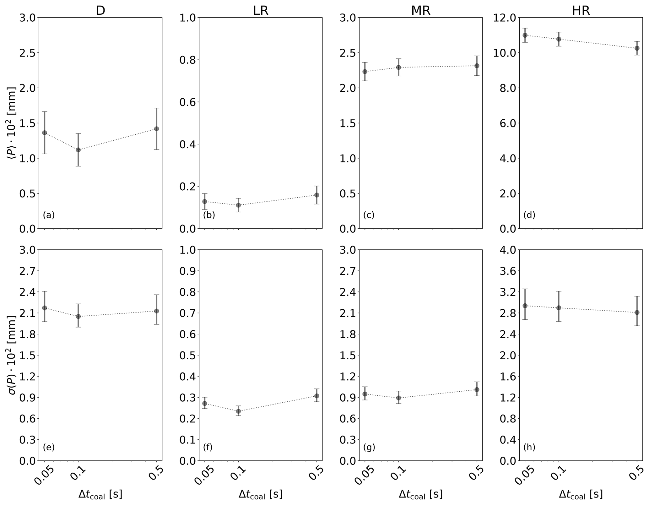
Figure 10Ensemble mean and standard deviation of accumulated precipitation at the end of a simulation against time step for coalescence in four scenarios of a CC simulation with . Error bars represent the 95 % confidence interval.
Mean surface precipitation for differing numbers of SDs is shown in Fig. 11. We find that 〈P〉 varies with in a nontrivial way, similar in all four scenarios. Mean precipitation is the highest for . Then, there is a large decrease in 〈P〉 when is increased from 10 to 50. A minimum of 〈P〉 is found between and , depending on the scenario. Beyond this minimum, 〈P〉 slowly increases (see panels e–h). In the D and HR scenarios, there is evidence for convergence of 〈P〉 for and for , respectively. Above these values, centers of confidence intervals are at similar positions and the intervals overlap. In the LR and MR scenarios, the center of the confidence interval increases for . Although the intervals often overlap, this systematic increase indicates that 〈P〉 has not converged.
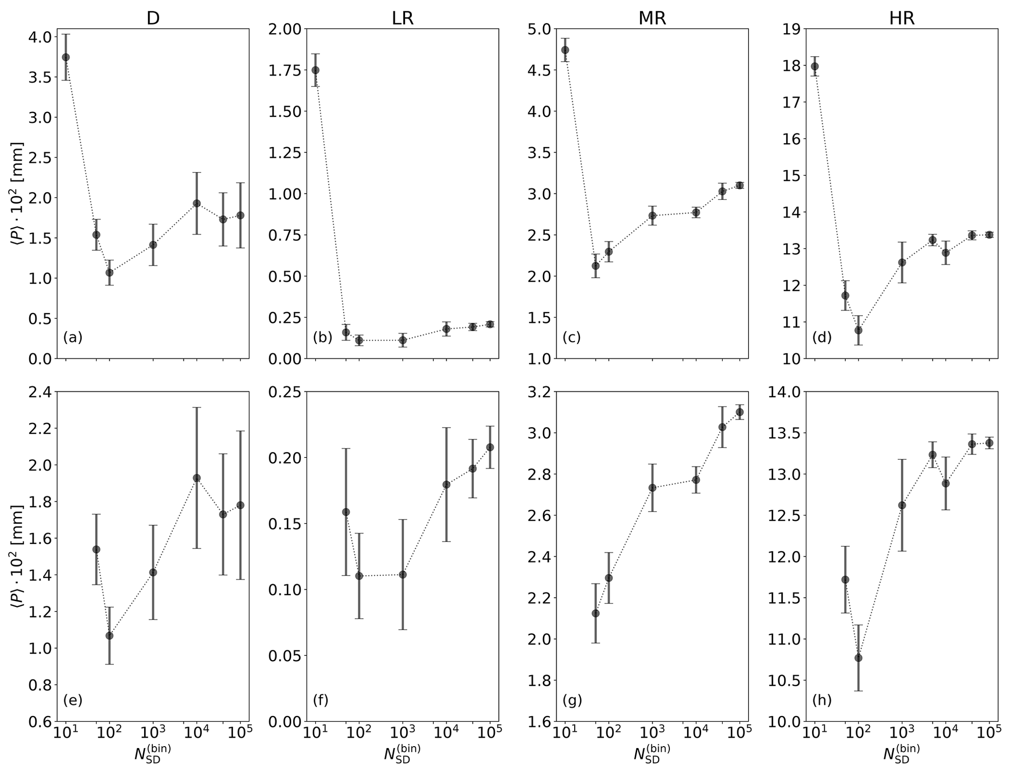
Figure 11Ensemble mean of precipitation against number of super-droplets for four scenarios: D, LR, MR, and HR. In (e)–(h) the same results are shown as in (a)–(d), but without . Error bars show the 95 % confidence interval.
Changes in 〈P〉 for are consistent with changes in the mean DSD in box simulations (see Fig. 3d). In box simulations, gives too few droplets with radii between 40 and 120 µm but too many droplets with radii greater than 120 µm. Since surface precipitation is sensitive to the largest droplets, this is consistent with 〈P〉 that is too large seen in CC simulations. For , the number of the largest droplets is no longer overestimated in box simulations, but there are still too few droplets with radii between 50 and 120 µm. This is consistent with a sharp decrease in 〈P〉 between and . In box simulations with the number of droplets with sizes between 50 and 120 µm is no longer underestimated, which is consistent with an increase in 〈P〉 between and in CC simulations.
The increase in 〈P〉 for , however, cannot be easily explained by box simulations or by CC simulations without collision–coalescence because mean results of these two simulation types converge for (see Sects. 3 and 5.4). This suggests that 〈P〉 may be affected by variance of the DSD that is too large, which does not converge in box simulations even for . The fact that 〈P〉 quickly converges with Δtcoal is consistent with this hypothesis because Δtcoal does not affect the variance of the DSD. Variance that is too large and a correct mean of the DSD in box simulations correspond to a situation in which LES differences between DSDs in neighboring cells are larger than expected. There are some cells with more large droplets than expected and some cells with fewer large droplets than expected. To show how the spatial distribution of rain within the cloud changes with , in Fig. 12 we show the probability density function of rainwater content at four points in time, from just before the onset of surface precipitation until its maximum. We find that the distribution narrows with increasing . For small , the distribution is bimodal, in particular at earlier times. As is increased, the smaller mode disappears, and we get a single mode, with a maximum for smaller values of rainwater content than the maximum of the larger of the two modes observed for small . The distribution converges for a similar value of as the one required for convergence of 〈P〉.
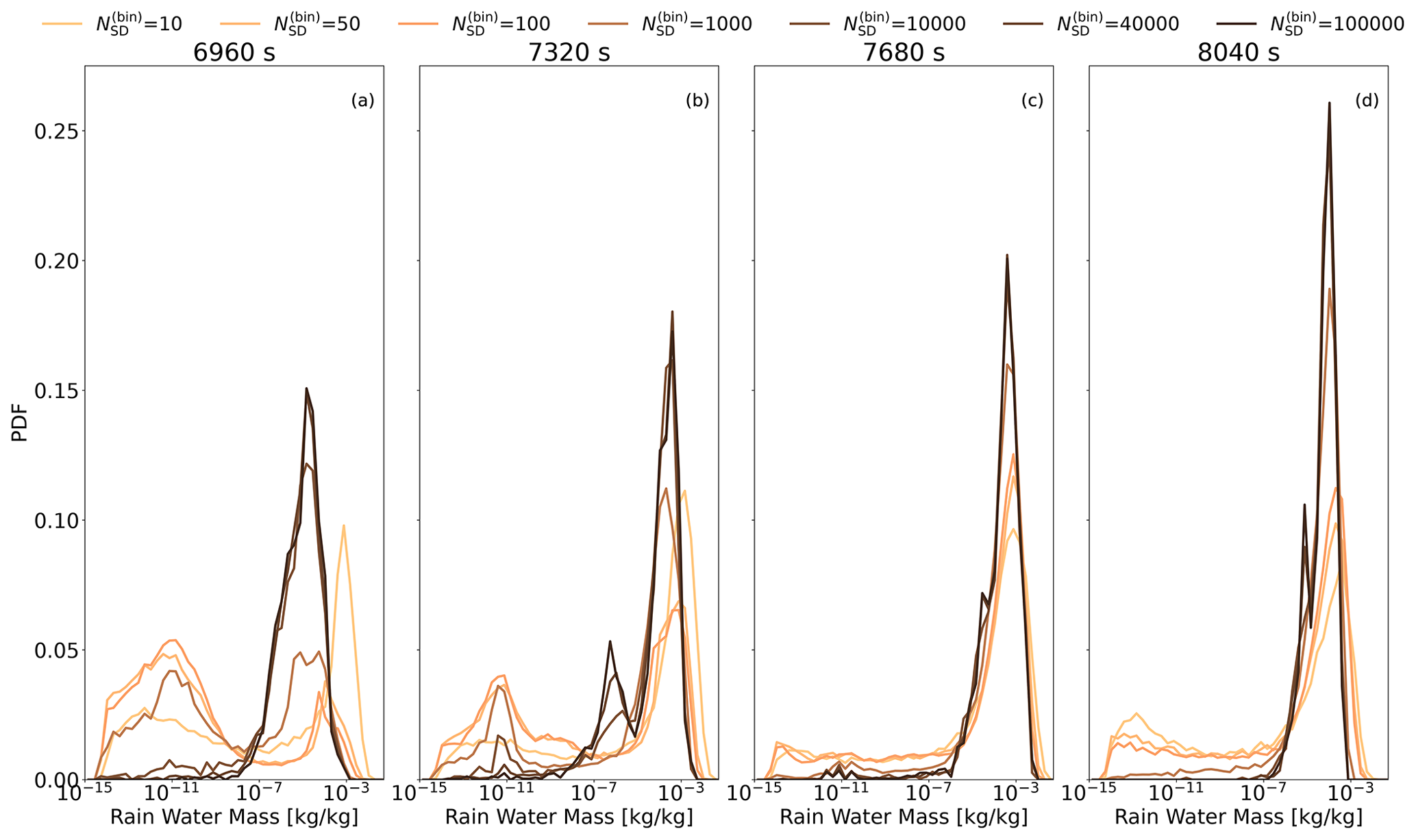
Figure 12Probability density function of rainwater mass in cloudy cells at four moments in time, averaged from the HR simulation ensemble.
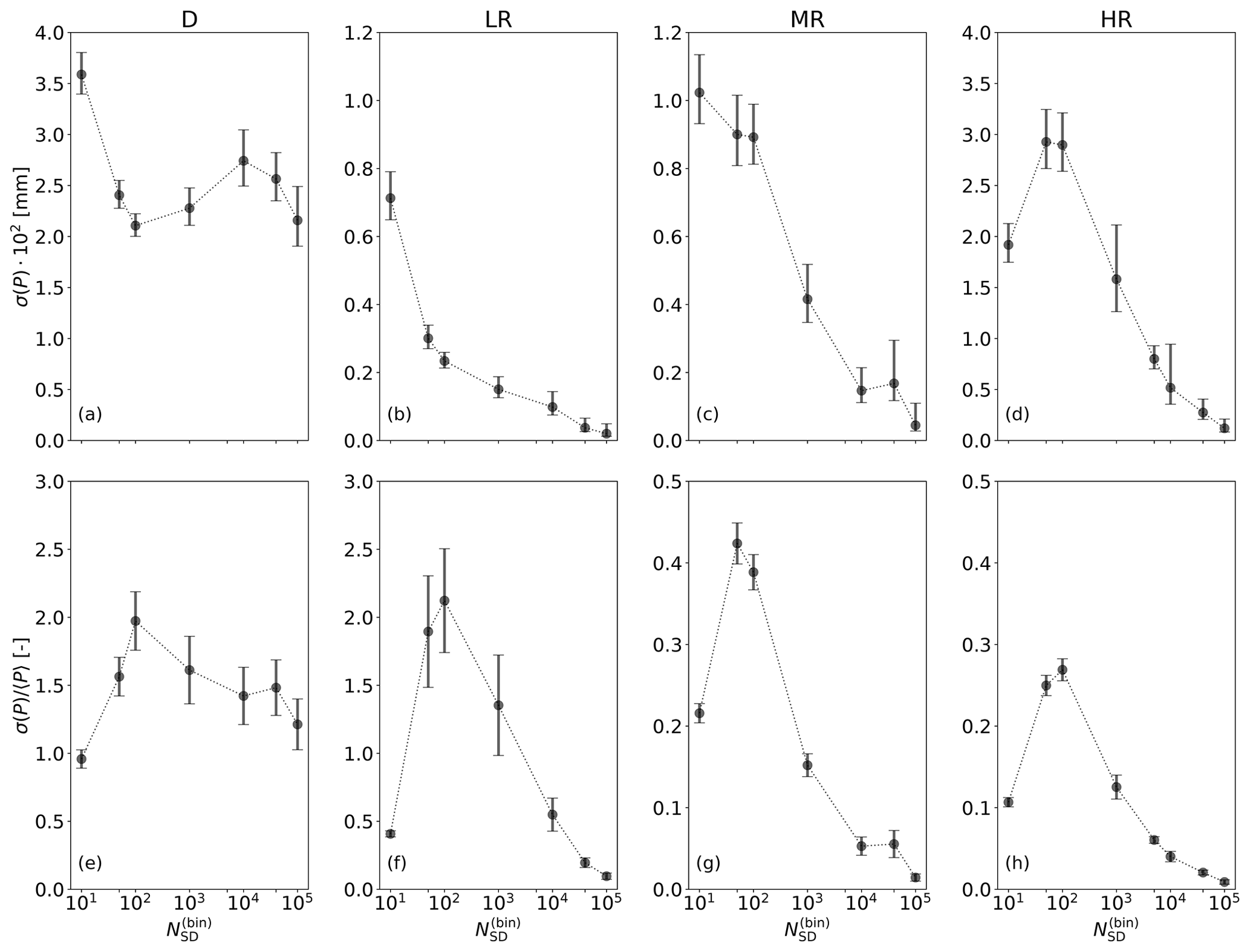
Figure 13Ensemble standard deviation (a–d) and relative standard deviation (e–h) of precipitation against the number of super-droplets for four types of simulations: D, LR, MR, and HR. In (a)–(d), error bars show the 95 % confidence interval. In (e)–(h), error bars show the error estimated with .
The standard deviation of precipitation for differing numbers of SDs is shown in Fig. 13. In dynamic simulations (panel a), σ(P) is large for , then sharply decreases for and does not change significantly as is further increased. Most of the 95 % confidence intervals overlap for . The relative standard deviation (panel e) is around 1.5 for . The relatively low sensitivity of σ(P) to in dynamic simulations shows that precipitation is more sensitive to differences in the flow field, which can be a consequence of small random perturbations of initial conditions, than to differences in realization of the collision–coalescence model of particle microphysics.
In kinematic simulations (panels b–d) the standard deviation of precipitation is more sensitive to than in dynamic simulations. There is a significant decrease in σ(P) as is increased (except for small in HR). The relative standard deviation has a maximum for between 50 and 100 and decreases for higher (panels f–h). This shows that in the absence of differences in flow field, precipitation is governed by realizations of the collision–coalescence model. Comparing D with MR, which is the kinematic case with the most similar 〈P〉, we find that in dynamic simulations is much larger than in kinematic simulations, from around 4 times larger for low to up to 70 times larger for large . This supports the conclusion that precipitation primarily depends on the realized flow field and not on the realization of AON.
5.6 Sensitivity to SD initialization method
Collision–coalescence in particle microphysics is sensitive to the way SD attributes are initialized. Therefore, the way precipitation changes with the number of SDs could depend on SD initialization. To check this, we test convergence for three types of SD initializations that were introduced in Sect. 2.1: ξconst-init, const SD-init, and const SD fixed-init. In const SD fixed-init the outermost bin edges for dry radius were set to 1 nm and 5 µm. For all methods, the initial DSD averaged over a large number of cells agrees very well with the prescribed distribution (Fig. 2a shows this, albeit for a different distribution). All methods give very good representation of the initial DSD. Comparison of results for different initialization methods in the HR case is shown in Fig. 14. We see only minor differences between const SD-init and const SD fixed-init. Both methods use bins to make sampling of the initial aerosol radius more even but differ in the way the entire bin range is selected. Recently, Hill et al. (2023) found differences in precipitation between different implementations of particle microphysics using both AON and binned initialization. Differences in details of bin initialization were proposed as one of potential reasons for the observed discrepancies. Good agreement between const SD-init and const SD fixed-init in our simulations suggests that some other factor is responsible for the discrepancies discussed in Hill et al. (2023).
The ξconst-init gives significantly different results than the bin initialization methods. In ξconst-init there is very little precipitation when is small. As more SDs are used, the amount of precipitation increases. It is plausible that all methods of initialization should converge for a large enough number of SDs. However, even for , which was the largest number of SDs that we were able to model in ξconst-init, ξconst-init gives less precipitation than the other methods. Unterstrasser et al. (2017) showed that ξconst-init requires a huge number of SDs in box simulations of collision–coalescence, and the authors hypothesized that it may require fewer SDs in cloud simulations. Our results show that this is not the case: in 2D simulations ξconst-init has the same deficiencies as in box simulations. It requires a very large number of super-droplets, which is unattainable in 3D LESs, to get convergence in precipitation. For fewer SDs, it gives significantly too little precipitation.
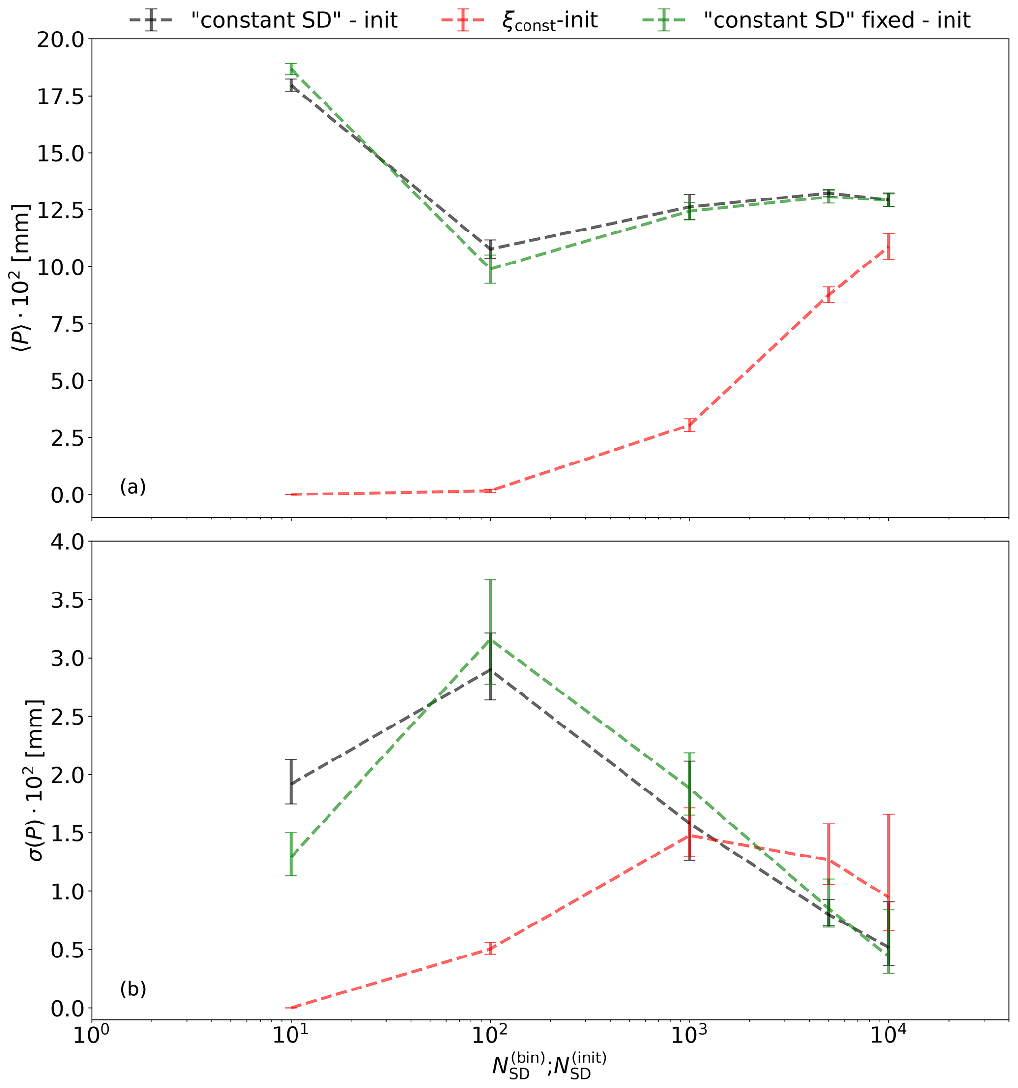
Figure 14Mean 〈P〉 and standard deviation σ(P) of accumulated precipitation against the number of SDs for HR simulations with three SD initialization methods. The horizontal axis is in constant SD-init and in ξconst-init. In constant SD fixed-init we have . Error bars represent the 95 % confidence interval.
5.7 Sensitivity to SGS motion of SDs
In multi-box simulations, mixing of droplets between cells helps achieve convergence of collision–coalescence modeling. In CC simulations discussed so far, intercell mixing was caused by the resolved-scale motion and by sedimentation, but there was no SGS motion of SDs. Here, we consider simulations in which SGS velocity of SDs is modeled using the OU method, which should make mixing more efficient. In the OU model, we assume a constant and uniform TKE dissipation rate of 5 cm2 s−3. Subgrid-scale motion can increase the number of SDs that hit the bottom wall of the domain, resulting in a decrease in the number of SDs and in aerosol concentration. This complicates the comparison with simulations without SGS motion of SDs. Therefore, in simulations with the OU model we compensate for aerosol depletion by adding SDs whenever there are fewer aerosols than at the simulation start. Details of the procedure can be found in Dziekan et al. (2021). This relaxation is done only in the lowest 700 m of the domain, below the cloud base. Parameters of relaxation were tuned to get the SD number and aerosol concentration close to those in simulations without SGS motion of SDs. Histograms with the number of SDs in cloudy cells and vertical profiles of several parameters, including aerosol concentration, are shown in the Supplement. Convergence of precipitation statistics with and without the OU model is compared in Fig. 15. We do not see any significant effect of SGS motion. In HR, mean precipitation agrees very well. In D, there are small differences, but 〈P〉 changes with similarly with and without the OU model. As we did not observe any impact of SGS SD motion for , we did not test higher .
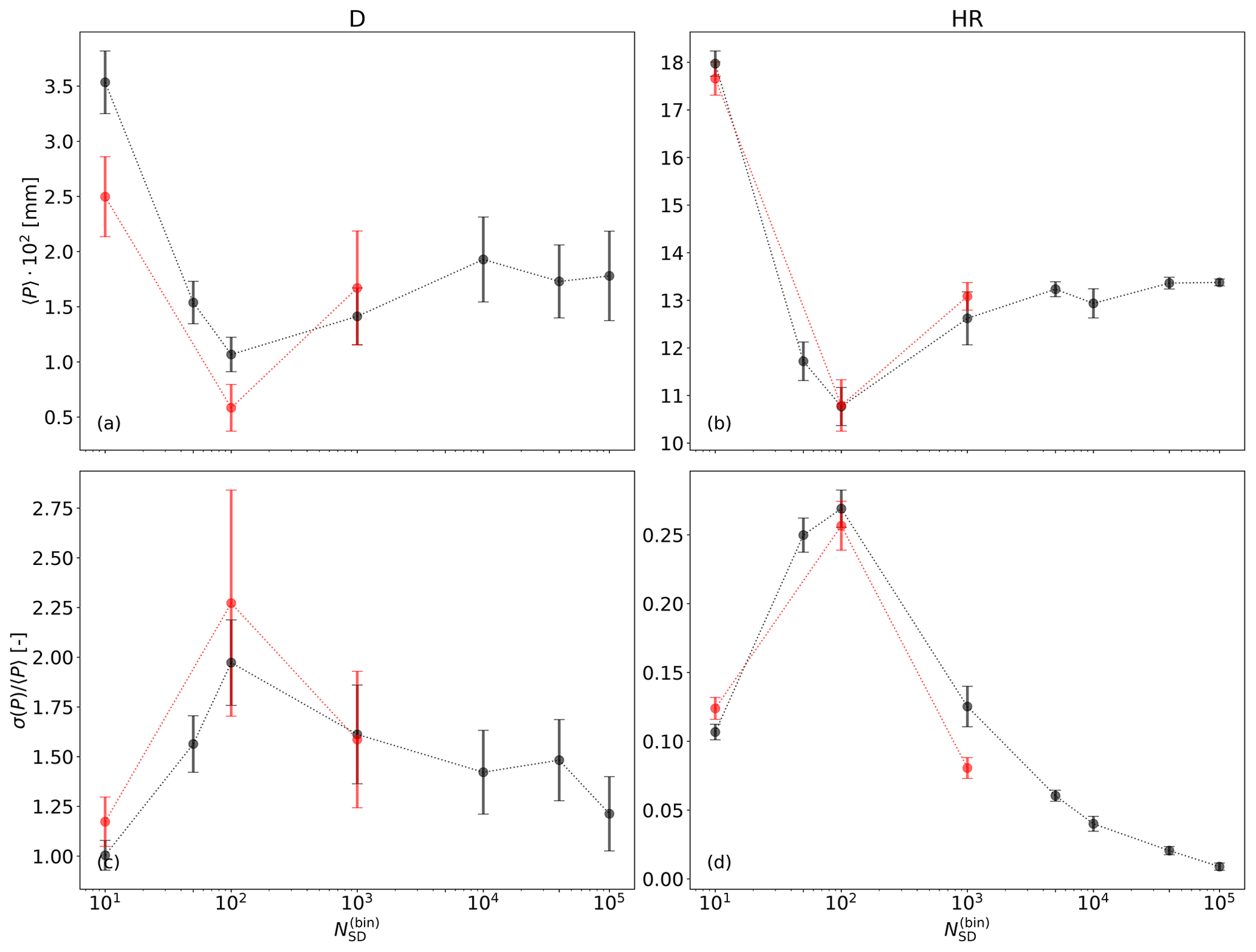
Figure 15Mean and relative standard deviation of accumulated precipitation against the number of SDs for simulations with (red) and without (black) the OU model of SGS motion of SDs.
Our study shows that using particle microphysics it is more difficult to reach numerical convergence of precipitation in cloud simulations than it is to reach convergence of mean DSD in an ensemble of box or multi-box simulations of collision–coalescence. In general, convergence requirements are less strict in strongly precipitating clouds than in lightly precipitating clouds.
It is relatively easy to have convergence with Δtcoal. Mean precipitation in our isolated cumulus simulations converged for Δtcoal=0.5 s. The same time step length was also sufficient in simulations of cumulus cloud fields (Dziekan et al., 2021). However, box simulations presented in this text and stratocumulus cloud field simulations from Dziekan et al. (2021) required Δtcoal=0.1 s. This suggests that Δtcoal=0.1 s is a safe choice for cloud modeling. We used the linear sampling technique. Quadratic sampling may allow for longer time steps (Unterstrasser et al., 2020). Variance of precipitation in cloud simulations and variance of the DSD in box simulation are not sensitive to Δtcoal.
It is more difficult to reach convergence with the number of SDs per cell. In box simulations, mean DSD converges for , but variance of the DSD decreases with without converging. In multi-box simulations (multiple boxes with mixing between them) mean DSD converges for fewer SDs than in box simulations, which is attributed to a positive role of intercell mixing. In cumulus simulations, mean precipitation converges for in the most heavily precipitating kinematic case and for in dynamic simulations. In kinematic cases with less precipitation, we do not see convergence of mean precipitation even for .
It is not clear why convergence is slower in CC than in box simulations. In CC, convergence of mean precipitation coincides with convergence of the spatial distribution of rain. This may suggest that mean precipitation is dependent on the spatial distribution of droplet sizes, probably because of interaction between cells. However, in multi-box simulations we observe that intercell mixing helps reach convergence. Increasing the rate of intercell mixing in CC by using an SGS model does not help with convergence. This does not necessarily indicate that intercell mixing is not important for convergence in CC. It is possible that the increase in intercell mixing caused by the SGS model is small in relation to intercell mixing caused by resolved eddies and by sedimentation. Precipitation is sensitive to the super-droplet initialization procedure. In this study initial radii were almost evenly distributed on a logarithmic scale. If droplet radii are randomly drawn from the initial distribution, it is more difficult to reach convergence with , and using that is too small induces larger errors. Note that the splitting–merging algorithm of Schwenkel et al. (2018), which was not included in this study, could help achieve convergence.
Variance of precipitation in an ensemble of cloud simulations decreases with , but only if the same flow field is used in the ensemble. If the flow field is different in different simulations, e.g., due to random perturbations of initial conditions, variance of precipitation is not sensitive to . This shows that in a typical LES, the increased variance in the number of collisions in particle microphysics does not affect variability in rain between simulation runs because differences in realized flow fields are more important.
In multi-box simulations, incompressible isotropic turbulence is modeled as a sum of random Fourier modes. The model is similar to that used in Sidin et al. (2009), but the generated velocity field is periodic because of the boundary conditions in multi-box simulations. We shall assume periodic boundary conditions in the space variable ,
for all x, y, and z as well as all signed integers nx ,ny, and nz, where L is called the period. It is enough to consider the restriction of the flow into a periodic cubic box of side L. Using Fourier series we write the velocity field as
with
Using the incompressibility condition and since u(r,t) is real-valued, the velocity field (Eq. A2) reduces to
where is the unit vector in the direction of k and M(n) is the n-dependent multiplicity (or degeneracy) of wave vectors kn,m with the same magnitude . For a given value of n (numbering the magnitude ), the index m numbers the wave vectors kn,m with
The time evolution of the random vector coefficients an,m(t) and bn,m(t) reads
for . In the expression above, ξa and ξb are independent random vectors, with components taken from a Gaussian distribution with zero mean and unit variance. The values of an,m(t) and bn,m(t) for m<0 are obtained from
The remaining quantities are the relaxation function
with frequencies
the Kolmogorov energy spectrum in the inertial subrange
variances
and differences in wave vector magnitudes
Validity of the periodic model is tested by comparing pair separation statistics with results from the non-periodic model of Sidin et al. (2009). Initial pair separation is equal to the Kolmogorov length assumed to be η=1 mm. The size of the largest eddies is L=1 m. In the non-periodic model, 200 wave vector magnitudes were used that form a geometric series between L and η (Sidin et al., 2009). For each wave vector magnitude, 50 wave vectors were randomly selected. In the periodic model, we used magnitudes of all periodic wave vectors between L and η. For each wave vector magnitude, n we randomly selected wave vectors, where M(n) is degeneracy. Time step was 0.1 s. Results are plotted in Fig. A1. We find that pair separation in the periodic model is somewhat larger. However, given that the choice of ϵ in multi-box tests is arbitrary, we decide that the periodic model is sufficiently realistic.
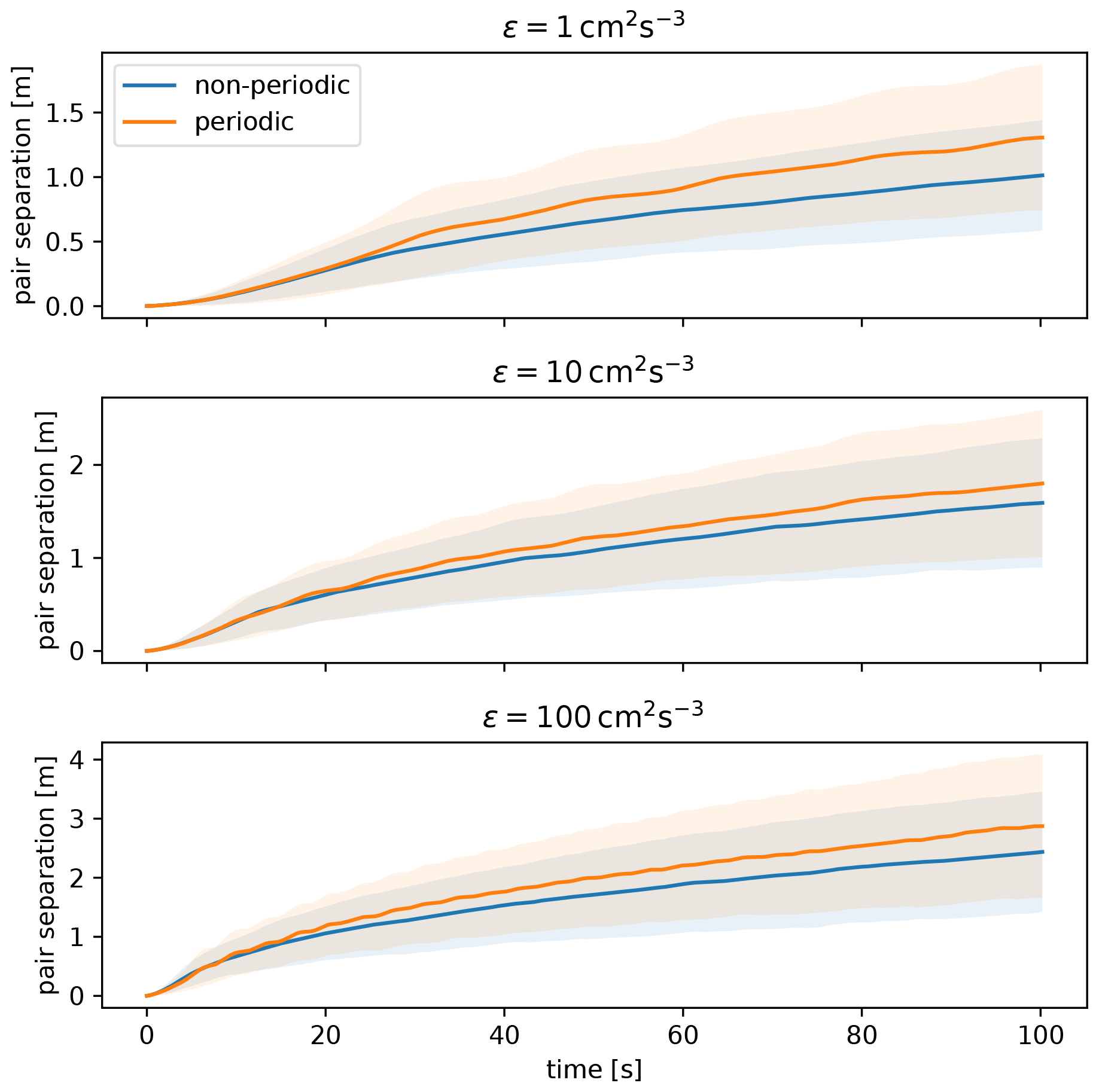
Figure A1Pair separation statistics from the periodic and non-periodic synthetic turbulence models for different values of the TKE dissipation rate. Solid lines show the ensemble mean, and shading shows 1 standard deviation interval.
Cloud simulations were done using UWLCM, and box and multi-box simulations were done with coal_fluctu. These models use the SDM implementation from the libcloudph++ library (Arabas et al., 2015). UWLCM also uses the libmpdata++ library (Jaruga et al., 2015). Plotting of UWLCM results was done with the UWLCM_plotting package. Pair separation tests were done using synth_turb. In the study, the following code versions were used: UWLCM v2.1 (https://doi.org/10.5281/zenodo.7643309, Dziekan et al., 2023), libmpdata++ v2.1 (https://doi.org/10.5281/zenodo.7643674, Arabas et al., 2023b), libcloudph++ v3.1 (https://doi.org/10.5281/zenodo.7643319, Arabas et al., 2023a), UWLCM_plotting v1.0 (https://doi.org/10.5281/zenodo.7643747, Dziekan and Zmijewski, 2023), coal_fluctu v2.2 (https://doi.org/10.5281/zenodo.10076329, Dziekan, 2023a), synth_turb v0.1 (https://doi.org/10.5281/zenodo.8270196, Dziekan, 2023b). Dataset, run scripts, and plotting scripts are available at https://doi.org/10.5281/zenodo.7685538 (Zmijewski et al., 2023).
The supplement related to this article is available online at: https://doi.org/10.5194/gmd-17-759-2024-supplement.
PZ and PD conceived the idea of the study. Simulations, analyses, and data visualization were done by PZ for CC simulations and by PD for box and multi-box simulations. All authors contributed to the paper. Funding was secured by PD and HP.
The contact author has declared that none of the authors has any competing interests.
Publisher's note: Copernicus Publications remains neutral with regard to jurisdictional claims made in the text, published maps, institutional affiliations, or any other geographical representation in this paper. While Copernicus Publications makes every effort to include appropriate place names, the final responsibility lies with the authors.
We thank Gustavo Abade for help with the periodic synthetic turbulence model and its description. We gratefully acknowledge Poland's high-performance infrastructure PLGrid (HPC centers: ACK Cyfronet AGH, PCSS, CI TASK, WCSS) for providing computer facilities and support under computational grant no. PLG/2022/015886. The calculations were made with the support of the Interdisciplinary Center for Mathematical and Computational Modeling of the University of Warsaw (ICM UW) under computational grant no. GR84-48.
This research has been supported by the Polish National Science Center (grant nos. 2018/31/D/ST10/01577 and 2016/23/B/ST10/00690).
This paper was edited by Simon Unterstrasser and reviewed by Yign Noh and one anonymous referee.
Andrejczuk, M., Grabowski, W. W., Reisner, J., and Gadian, A.: Cloud-aerosol interactions for boundary layer stratocumulus in the Lagrangian Cloud Model, J. Geophys. Res.-Atmos., 115, D22214, https://doi.org/10.1029/2010JD014248, 2010. a
Arabas, S. and Shima, S. I.: Large-eddy simulations of trade wind cumuli using particle-based microphysics with monte Carlo coalescence, J. Atmos. Sci., 70, 2768–2777, https://doi.org/10.1175/JAS-D-12-0295.1, 2013. a
Arabas, S., Jaruga, A., Pawlowska, H., and Grabowski, W. W.: libcloudph++ 1.0: a single-moment bulk, double-moment bulk, and particle-based warm-rain microphysics library in C++, Geosci. Model Dev., 8, 1677–1707, https://doi.org/10.5194/gmd-8-1677-2015, 2015. a, b
Arabas, S., Jaruga, A., Dziekan, P., Waruszewski, M., and Jarecka, D.: libcloudph++ v3.1 source code, Zenodo [code], https://doi.org/10.5281/zenodo.7643319, 2023a. a
Arabas, S., Waruszewski, M., Dziekan, P., Jaruga, A., Jarecka, D., Badger, C., and Singer, C.: libmpdata++ v2.1 source code, Zenodo [code], https://doi.org/10.5281/zenodo.7643674, 2023b. a
Arakawa, A. and Lamb, V. R.: Computational Design of the Basic Dynamical Processes of the UCLA General Circulation Model, General circulation models of the atmosphere, Methods in Computational Physics: Advances in Research and Applications, 17, 173–265, https://doi.org/10.1016/b978-0-12-460817-7.50009-4, 1977. a
Bott, A.: An efficient numerical flux method for the solution of the stochastic collection equation, J. Aerosol Sci., 28, 2284–2293, https://doi.org/10.1016/S0021-8502(97)85371-2, 1997. a
Davis, M. H.: Collisions of Small Cloud Droplets: Gas Kinetic Effects, J. Atmos. Sci., 29, 911–915, https://doi.org/10.1175/1520-0469(1972)029<0911:coscdg>2.0.co;2, 1972. a, b
Dziekan, P.: Coal Fluctu v2.2 source code, Zenodo [code], https://doi.org/10.5281/zenodo.10076329, 2023a. a
Dziekan, P.: igfuw/synth_turb: Initial release, Zenodo [code], https://doi.org/10.5281/zenodo.8270196, 2023b. a
Dziekan, P. and Pawlowska, H.: Stochastic coalescence in Lagrangian cloud microphysics, Atmos. Chem. Phys., 17, 13509–13520, https://doi.org/10.5194/acp-17-13509-2017, 2017. a, b, c, d, e, f, g, h, i, j, k, l, m, n, o, p
Dziekan, P. and Zmijewski, P.: University of Warsaw Lagrangian Cloud Model (UWLCM) 2.0: adaptation of a mixed Eulerian–Lagrangian numerical model for heterogeneous computing clusters, Geosci. Model Dev., 15, 4489–4501, https://doi.org/10.5194/gmd-15-4489-2022, 2022. a
Dziekan, P. and Zmijewski, P.: UWLCM plotting v1.0 source code, Zenodo [code], https://doi.org/10.5281/zenodo.7643747, 2023. a
Dziekan, P., Waruszewski, M., and Pawlowska, H.: University of Warsaw Lagrangian Cloud Model (UWLCM) 1.0: a modern large-eddy simulation tool for warm cloud modeling with Lagrangian microphysics, Geosci. Model Dev., 12, 2587–2606, https://doi.org/10.5194/gmd-12-2587-2019, 2019. a, b
Dziekan, P., Jensen, J. B., Grabowski, W. W., and Pawlowska, H.: Impact of Giant Sea Salt Aerosol Particles on Precipitation in Marine Cumuli and Stratocumuli: Lagrangian Cloud Model Simulations, J. Atmos. Sci., 78, 4127–4142, https://doi.org/10.1175/JAS-D-21-0041.1, 2021. a, b, c, d
Dziekan, P., Singer, C., Waruszewski, M., Jaruga, A., and Zmijewski, P.: University of Warsaw Lagrangian Cloud Model v2.1 source code, Zenodo [code], https://doi.org/10.5281/zenodo.7643309, 2023. a
Gillespie, D. T.: Exact Method for Numerically Simulating the Stochastic Coalescence Process in a Cloud, J. Atmos. Sci., 32, 1977–1989, https://doi.org/10.1175/1520-0469(1975)032<1977:AEMFNS>2.0.CO;2, 1975. a, b, c, d
Grabowski, W. W.: Comparison of eulerian bin and lagrangian particle-based microphysics in simulations of nonprecipitating cumulus, J. Atmos. Sci., 77, 3951–3970, https://doi.org/10.1175/JAS-D-20-0100.1, 2020. a
Grabowski, W. W. and Abade, G. C.: Broadening of cloud droplet spectra through eddy hopping: Turbulent adiabatic parcel simulations, J. Atmos. Sci., 74, 1485–1493, https://doi.org/10.1175/JAS-D-17-0043.1, 2017. a
Grinstein, F. F., Margolin, L. G., and Rider, W. J.: Implicit large eddy simulation: Computing turbulent fluid dynamics, vol. 9780521869, Cambridge University Press, ISBN 9780511618604, 2007. a
Hall, W. D.: A Detailed Microphysical Model Within a Two-Dimensional Dynamic Framework: Model Description and Preliminary Results, J. Atmos. Sci., 37, 2486–2507, https://doi.org/10.1175/1520-0469(1980)037<2486:admmwa>2.0.co;2, 1980. a, b
Hill, A. A., Lebo, Z. J., Andrejczuk, M., Arabas, S., Dziekan, P., Field, P., Gettelman, A., Hoffmann, F., Pawlowska, H., Onishi, R., and Vié, B.: Toward a Numerical Benchmark for Warm Rain Processes, J. Atmos. Sci., 80, 1329–1359, https://doi.org/10.1175/JAS-D-21-0275.1, 2023. a, b, c
Hoffmann, F. and Feingold, G.: Cloud Microphysical Implications for Marine Cloud Brightening: The Importance of the Seeded Particle Size Distribution, J. Atmos. Sci., 78, 3247–3262, https://doi.org/10.1175/JAS-D-21-0077.1, 2021. a
Hoffmann, F., Raasch, S., and Noh, Y.: Entrainment of aerosols and their activation in a shallow cumulus cloud studied with a coupled LCM-LES approach, Atmos. Res., 156, 43–57, https://doi.org/10.1016/j.atmosres.2014.12.008, 2015. a
Jaruga, A., Arabas, S., Jarecka, D., Pawlowska, H., Smolarkiewicz, P. K., and Waruszewski, M.: libmpdata++ 1.0: a library of parallel MPDATA solvers for systems of generalised transport equations, Geosci. Model Dev., 8, 1005–1032, https://doi.org/10.5194/gmd-8-1005-2015, 2015. a
Khvorostyanov, V. I. and Curry, J. A.: Terminal velocities of droplets and crystals: Power laws with continuous parameters over the size spectrum, J. Atmos. Sci., 59, 1872–1884, https://doi.org/10.1175/1520-0469(2002)059<1872:TVODAC>2.0.CO;2, 2002. a
Lasher-Trapp, S. G., Knight, C. A., and Straka, J. M.: Early Radar Echoes from Ultragiant Aerosol in a Cumulus Congestus: Modeling and Observations, J. Atmos. Sci., 58, 3545–3562, https://doi.org/10.1175/1520-0469(2001)058<3545:EREFUA>2.0.CO;2, 2001. a
Lipps, F. B. and Hemler, R. S.: A scale analysis of deep moist convection and some related numerical calculations., J. Atmos. Sci., 39, 2192–2210, https://doi.org/10.1175/1520-0469(1982)039<2192:ASAODM>2.0.CO;2, 1982. a
Lu, C., Niu, S., Liu, Y., and Vogelmann, A. M.: Empirical relationship between entrainment rate and microphysics in cumulus clouds, Geophys. Res. Lett., 40, 2333–2338, https://doi.org/10.1002/grl.50445, 2013. a
Miles, N. L., Verlinde, J., and Clothiaux, E. E.: Cloud Droplet Size Distributions in Low-Level Stratiform Clouds, J. Atmos. Sci., 57, 295–311, https://doi.org/10.1175/1520-0469(2000)057<0295:CDSDIL>2.0.CO;2, 2000. a
Onishi, R., Matsuda, K., and Takahashi, K.: Lagrangian tracking simulation of droplet growth in turbulence-turbulence enhancement of autoconversion rate, J. Atmos. Sci., 72, 2591–2607, https://doi.org/10.1175/JAS-D-14-0292.1, 2015. a
Pawlowska, H., Grabowski, W. W., and Brenguier, J.-L.: Observations of the width of cloud droplet spectra in stratocumulus, Geophys. Res. Lett., 33, L19810, https://doi.org/10.1029/2006GL026841, 2006. a
Rao, C. R.: Linear Statistical Inference and its Applications, Wiley, https://doi.org/10.1002/9780470316436, 1973. a
Riechelmann, T., Noh, Y., and Raasch, S.: A new method for large-eddy simulations of clouds with Lagrangian droplets including the effects of turbulent collision, New J. Phys., 14, 65008, https://doi.org/10.1088/1367-2630/14/6/065008, 2012. a
Schwenkel, J., Hoffmann, F., and Raasch, S.: Improving collisional growth in Lagrangian cloud models: development and verification of a new splitting algorithm, Geosci. Model Dev., 11, 3929–3944, https://doi.org/10.5194/gmd-11-3929-2018, 2018. a, b, c, d
Sheskin, D. J.: Handbook of Parametric and Nonparametric Statistical Procedures, 5th edn., Chapman and Hall/CRC, https://doi.org/10.1201/9780429186196, 2011. a
Shima, S., Kusano, K., Kawano, A., Sugiyama, T., and Kawahara, S.: The super-droplet method for the numerical simulation of clouds and precipitation: A particle-based and probabilistic microphysics model coupled with a non-hydrostatic model, Q. J. Roy. Meteor. Soc., 135, 1307–1320, https://doi.org/10.1002/qj.441, 2009. a, b, c, d, e, f, g, h, i, j, k, l, m, n, o
Shima, S., Sato, Y., Hashimoto, A., and Misumi, R.: Predicting the morphology of ice particles in deep convection using the super-droplet method: development and evaluation of SCALE-SDM 0.2.5-2.2.0, -2.2.1, and -2.2.2, Geosci. Model Dev., 13, 4107–4157, https://doi.org/10.5194/gmd-13-4107-2020, 2020. a
Sidin, R. S., IJzermans, R. H., and Reeks, M. W.: A Lagrangian approach to droplet condensation in atmospheric clouds, Phys. Fluids, 21, 106603, https://doi.org/10.1063/1.3244646, 2009. a, b, c
Smolarkiewicz, P. K.: Multidimensional positive definite advection transport algorithm: an overview, Int. J. Numer. Meth. Fl., 50, 1123–1144, https://doi.org/10.1002/fld.1071, 2006. a
Smolarkiewicz, P. K. and Margolin, L.: Variational methods for elliptic problems in fluid models, in: Workshop on Developments in Numerical Methods for Very High resolution global models, Reading, UK, 5–7 June 2000, 137–159, https://www.ecmwf.int/en/elibrary/76465-variational-methods-elliptic-problems-fluid-models (last access: 26 January 2024), 2000. a
Sölch, I. and Kärcher, B.: A large-eddy model for cirrus clouds with explicit aerosol and ice microphysics and Lagrangian ice particle tracking, Q. J. Roy. Meteor. Soc., 136, 2074–2093, https://doi.org/10.1002/qj.689, 2010. a
Unterstrasser, S., Hoffmann, F., and Lerch, M.: Collection/aggregation algorithms in Lagrangian cloud microphysical models: rigorous evaluation in box model simulations, Geosci. Model Dev., 10, 1521–1548, https://doi.org/10.5194/gmd-10-1521-2017, 2017. a, b, c, d, e, f, g, h, i, j, k, l, m, n, o, p, q, r, s
Unterstrasser, S., Hoffmann, F., and Lerch, M.: Collisional growth in a particle-based cloud microphysical model: insights from column model simulations using LCM1D (v1.0), Geosci. Model Dev., 13, 5119–5145, https://doi.org/10.5194/gmd-13-5119-2020, 2020. a, b, c, d, e, f, g, h, i, j, k, l, m
VanZanten, M. C., Stevens, B., Nuijens, L., Siebesma, A. P., Ackerman, A. S., Burnet, F., Cheng, A., Couvreux, F., Jiang, H., Khairoutdinov, M., Kogan, Y., Lewellen, D. C., Mechem, D., Nakamura, K., Noda, A., Shipway, B. J., Slawinska, J., Wang, S., and Wyszogrodzki, A.: Controls on precipitation and cloudiness in simulations of trade-wind cumulus as observed during RICO, J. Adv. Model. Earth Sy., 3, M06001, https://doi.org/10.1029/2011MS000056, 2011. a
Zmijewski, P., Dziekan, P., and Pawlowska, H.: Data and scripts accompanying the paper “Modeling Collision-Coalescence in Particle Microphysics: Numerical Convergence of Mean and Variance of Precipitation in Cloud Simulations Using University of Warsaw Lagrangian Cloud Model (UWLCM) 2.1”, Zenodo [data set], https://doi.org/10.5281/zenodo.7685538, 2023. a
- Abstract
- Introduction
- Particle microphysics
- Box simulations
- Multi-box simulations
- 2D cumulus congestus simulations
- Conclusions
- Appendix A: Periodic synthetic turbulence model
- Code and data availability
- Author contributions
- Competing interests
- Disclaimer
- Acknowledgements
- Financial support
- Review statement
- References
- Supplement