Improved definition of prior uncertainties in CO₂ and CO fossil fuel fluxes and its impact on multi-species inversion with GEOS-Chem (v12.5)

Monitoring, reporting, and verification frameworks for greenhouse gas emissions are being developed by countries across the world to keep track of progress towards national emission reduction targets. Data assimilation plays an important role in monitoring frameworks, combining different sources of information to achieve the best possible estimate of fossil fuel emissions and, as a consequence, better estimates for fluxes from the natural biosphere. Robust estimates for fossil fuel emissions rely on accurate estimates of uncertainties corresponding to different pieces of information. We describe prior uncertainties in CO₂ and CO fossil fuel fluxes, paying special attention to spatial error correlations and the covariance structure between CO₂ and CO. This represents the first time that prior uncertainties in CO₂ and the important co-emitted trace gas CO are defined consistently, with error correlations included, which allows us to make use of the synergy between the two trace gases to better constrain CO₂ fossil fuel fluxes. CO:CO₂ error correlations differ by sector, depending on the diversity of sub-processes occurring within a sector, and also show a large range of values between pixels within the same sector. For example, for other stationary combustion, pixel correlation values range from 0.1 to 1.0, whereas for road transport, the correlation is mostly larger than 0.6. We illustrate the added value of our definition of prior uncertainties using closed-loop numerical experiments over mainland Europe and the UK, which isolate the influence of using error correlations between CO₂ and CO and the influence of prescribing more detailed information about prior emission uncertainties. For the experiments, synthetic in situ observations are used, allowing us to validate the results against a “truth”. The “true” emissions are made by perturbing the prior emissions (from an emission inventory) according to the prescribed prior uncertainties. We find that using our realistic definition of prior uncertainties helps our data assimilation system to differentiate more easily between CO₂ fluxes from biogenic and fossil fuel sources. Using improved prior emission uncertainties, we find fewer geographic regions with significant deviations from the prior compared to when using default prior uncertainties (32 vs. 80 grid cells of 0.25°×0.3125°, with an absolute difference of more than 1 kg s⁻¹ between the prior and posterior), but these deviations from the prior almost consistently move closer to the prescribed true values, with 92 % showing an improvement, in contrast to the default prior uncertainties, where 61 % show an improvement. We also find that using CO provides additional information on CO₂ fossil fuel fluxes, but this is only the case if the CO:CO₂ error covariance structure is defined realistically. Using the default prior uncertainties, the CO₂ fossil fuel fluxes move farther away from the truth in many geographical regions (with 50 % showing an improvement compared to 94 % when advanced prior uncertainties are used). With the default uncertainties, the maximum deviation of fossil fuel CO₂ from the prescribed truth is about 7 % in both the prior and posterior results. With the advanced uncertainties, this is reduced to 3 % in the posterior results.

1 Introduction

With the signing of the Paris Agreement, 195 nations have committed themselves to reducing their greenhouse gas (GHG) emissions. This calls for active monitoring of emissions and emission trends to ensure climate plans are being met. Work is currently ongoing to build a GHG monitoring, reporting, and verification (MRV) framework, which will track and verify emissions of the major GHGs using a multi-tiered observing system. The MRV framework will support the 5-yearly global stocktake (Balsamo et al., 2021; Janssens-Maenhout et al., 2020; Petrescu et al., 2021) and increase understanding of emission landscapes and the associated dominant source sectors that are necessary for developing effective nationwide emission mitigation strategies to support nationally determined contributions.

An important aspect of the MRV framework involves combining different types of data, e.g. spatially disaggregated bottom-up inventories, atmospheric data, and near-real-time weather and economic data, to obtain the best possible estimate of national fossil fuel GHG emissions. This is often done through data assimilation (or inverse modelling), which is a rigorous mathematical framework that combines all these pieces of information (Lauvaux et al., 2016; Pillai et al., 2016; Staufer et al., 2016; Wu et al., 2018). GHG data assimilation uses state-of-the-art atmospheric transport models, prior information on GHG sources and sinks, observational data, and the uncertainties in each of these data sources. The uncertainties determine how much confidence is assigned to each of the components and thus how much information is taken from them, but some of these uncertainties, e.g. model transport uncertainties, are notoriously difficult to estimate. A limiting factor is often the lack of sufficient high-quality observations. Although a relatively dense GHG monitoring network exists in some regions, e.g. the UK, mainland Europe, and North America, many regions only have very sparse observations. Satellite data can significantly increase this coverage and have proven useful in specific cases. For an MRV framework targeting CO₂ from combustion, one major limitation of satellite data is that observations are atmospheric columns that include a large background concentration (Broquet et al., 2018; Chevallier et al., 2022; Palmer et al., 2008; Reuter et al., 2019).

One way to isolate the signal from combustion emissions is by exploiting the synergy between CO₂ and co-emitted species, such as CO and NO_x, which share the same combustion sources. Many countries have an air quality monitoring network, and many air pollutants are observed from space (e.g. CO and NO₂), benefitting from relatively short e-folding lifetimes (less than a few months) and consequently having a smaller background contribution. Hence, co-emitted species have a better spatiotemporal coverage than radiocarbon measurements, often seen as the most reliable independent constraint on fossil fuel CO₂ fluxes (Turnbull et al., 2009). Several studies have explored the correlation between CO₂ and co-emitted species and the additional constraint imposed by co-emitted species on CO₂ emissions, using both in situ and satellite data (Boschetti et al., 2018; Brioude et al., 2013; Palmer et al., 2022; Reuter et al., 2019; Silva et al., 2013; Turnbull et al., 2006; Yang et al., 2023). Co-emitted species have been used to separate fossil fuel CO₂ from biogenic CO₂ signals (Oney et al., 2017; Suntharalingam et al., 2004; Vardag et al., 2015), to estimate CO₂ emissions without CO₂ observations (Konovalov et al., 2016; Liu et al., 2020; Lopez et al., 2013), and to allocate CO₂ signals to specific emission sectors (Nathan et al., 2018; Super et al., 2020b; Turnbull et al., 2015). The latter makes use of the sector-specific emission ratio of CO₂ and co-emitted species.

Although there is promise in this multi-species approach, the emission ratios are uncertain and dynamic in space and time (Ammoura et al., 2016; Liñán-Abanto et al., 2021; Super et al., 2017; Wu et al., 2022), and they may even depend on human behaviour or meteorological conditions (Ammoura et al., 2014; Hall et al., 2020). The objective of data assimilation is to reduce the mismatch between posterior estimates and observations so that co-emitted species are only useful for informing CO₂ emissions if the uncertainties in the CO₂ emission estimates are larger than uncertainties associated with the observed ratios between CO₂ and co-emitted species. Therefore, an important role is laid out for accurately assessing the uncertainties in prior emissions and the definition of error correlations, which is a complex task. Gridded prior emissions are based on several data sources and therefore include uncertainties in activity data, emission factors (the amount of pollutant emitted per unit of activity), and spatial and temporal patterns. Some of these uncertainties might also be correlated, e.g. between regions and/or trace gases. Error correlations describe the synergy in emission uncertainties and can increase the amount of information gained from the same input data. One example is that gridded uncertainties are not independent of uncertainties in nearby grid cells.

In order to simultaneously optimize CO₂ and CO emissions, we need to make optimal use of these synergies. At the national scale, the most uncertain parameter is the CO emission factor. Unfortunately, the errors in the CO and CO₂ emission factors are not correlated, limiting the use of CO in constraining CO₂ at the national scale (Palmer et al., 2006). However, CO and CO₂ emissions are correlated through fossil fuel combustion activity, which determines, to a large extent, the spatial patterns of the emissions. In practice, the spatial distribution for CO and CO₂ emission estimates is often based on the same spatial data. Therefore, gridded CO and CO₂ emission estimates show a much stronger error correlation than national emissions. The relative error in CO₂ emissions for one grid cell is likely to be similar to the relative error in CO emissions for the same grid cell because the errors are caused by the assumed shared activity. Hence, by quantifying the gridded error correlations, we can make better use of the CO information to constrain CO₂.

Few studies have tried to estimate gridded emission uncertainties (Gately and Hutyra, 2017; Hogue et al., 2016; Hutchins et al., 2017; Oda et al., 2019), and they have only done so for CO₂. These studies mostly compare different emission datasets, which likely underestimate the uncertainties when the inventories use similar underlying data. Super et al. (2020a) provided a bottom-up uncertainty estimate of gridded emissions for CO₂ and CO using an emission inventory with a consistent methodology for CO₂ and co-emitted species. This increases the use of error correlations between CO₂ and co-emitted species. In this previous work, spatial errors were treated as independent, and no spatial correlations were considered. Also, the error correlation between CO₂ and co-emitted species was not examined.

Here, we describe an effort to build a consistent set of prior emission uncertainties for CO₂ and co-emitted species (CO), building further on the work done by Super et al. (2020a). This paper starts with a description of the data (Sect. 2.1) and methodology (Sect. 2.2) used to develop a more detailed definition of prior uncertainties, including spatial error correlation lengths and the error correlation between CO₂ and CO. The results are shown in Sect. 3.1. To illustrate the added value of well-defined information on prior uncertainties, we perform closed-loop numerical experiments, as explained in Sect. 2.3. We show the results for CO₂-only (Sect. 3.2) and multi-species inversions (Sect. 3.3).

2 Methods

This section starts with a description of the data used to make a detailed definition of prior uncertainties for gridded emissions, including the prior emission inventory. For this, we separate uncertainties in activity data, emission factors, and spatial patterns. Next, we describe the methodology used to estimate spatial error correlations and the error correlation between CO and CO₂. Additionally, we discuss how all uncertainties are combined into one product that can be used in data assimilation studies. Finally, we describe the setup of the inversions, including descriptions of the models, state vectors, input data, and different experiments.

In this work, we use the words “uncertainties” and “errors”, which have slightly different meanings. We do not know the exact errors in our data, so we talk about uncertainties to define how reliable our data are. When referring to correlations, we use the term “error”. For example, if errors between neighbouring grid cells are positively correlated, it means that if we overestimate a value for one grid cell, we are likely to do the same for neighbouring grid cells. In this case, we are talking about actual errors, which we cannot define but know are correlated. It is not the uncertainty that is correlated. For the same reason, we use the term “error covariance matrix”.

2.1 Prior data

2.1.1 European emission dataset

The European prior emission dataset used as a basis for this work is the TNO-GHGco-v4 inventory for 2018, with a spatial resolution of 0.1° by 0.05°, developed at the Netherlands Organisation for Applied Scientific Research (TNO). This dataset provides a unique set of consistent emissions for a range of GHGs and co-emitted species (Fig. 1), which allows us to study the impact of error correlations between these species on data assimilation studies.

Figure 1 TNO-GHGco-v4 emission maps of CO₂ and CO for 2018.

The TNO-GHGco-v4 dataset is similar to the CAMS-REG emission inventory (Kuenen et al., 2022), developed for the Copernicus Atmosphere Monitoring Service (CAMS), except that point sources are placed at their exact locations instead of being assigned to grid cells. It is compiled from emission reports delivered to the EMEP (European Monitoring and Evaluation Programme) Centre on Emission Inventories and Projections (Data reported by Parties under LRTAP Convention, 2022) and the United Nations Framework Convention on Climate Change (UNFCCC) (National Inventory Submissions 2020, 2022) by individual countries. The reports contain emissions for a long list of sub-sectors and fuels. In the final dataset, these emissions are aggregated into 12 sectors using GNFR (Gridded Nomenclature For Reporting) categorization (see Table 1). For countries that do not report their emissions, other emission datasets are used for gap filling, which are only available at the GNFR level. For the uncertainty estimates, we work with the detailed reported emission data. In the final product, we aggregate the data into six sectors: public power (GNFR A), industry (GNFR B), other stationary combustion (GNFR C), road transport (GNFR F), shipping (GNFR G), and a sixth group for the remaining minor GNFR sectors.

The country-level emissions are spatially downscaled to a 0.1° by 0.05° resolution using proxy maps (Kuenen et al., 2022). The proxy maps describe the fraction of the country-level emissions for a particular sub-sector that is assigned to one grid cell, ensuring that the fractions sum to 1 for each country-sector combination. Some proxy maps are used for multiple sub-sectors. For some countries, the spatial proxies are not available or are replaced with other datasets.

For shipping (GNFR G), a different approach is used because most of the emissions in this sector occur in international waters and are therefore not reported by countries. All shipping emissions are therefore taken directly from the Ship Traffic Emission Assessment Model (STEAM) (Jalkanen et al., 2012; Johansson et al., 2017), which provides gridded emissions using AIS (automatic identification system) data and vessel characteristics.

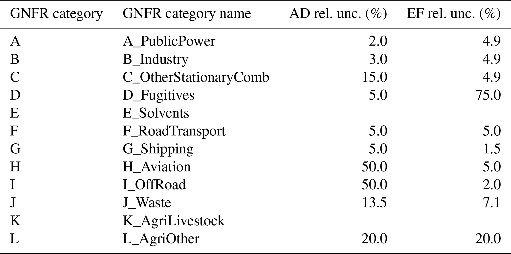
Table 1 An overview of the aggregated emission categories in the European emission data (GNFR) is provided, including relative uncertainties based on the Intergovernmental Panel on Climate Change (IPCC; 95 % confidence interval (CI)) in activity data (AD) and CO₂ emission factors (EFs) for each GNFR sector, which are used for countries without their own reporting. Note that “rel. unc.” stands for relative uncertainty.

2.1.2 Country-level emission uncertainties

In the emission reporting, over 250 different sector–fuel combinations are differentiated. We make a pre-selection of these by ordering the combinations based on their total emissions for the entire European domain. Then, we select the most important sector–fuel combinations until we have included at least 95 % of the emissions for all species. We combine the selections for all species, ensuring they are all the same, and we end up with 90 sector–fuel combinations that describe 96 % of CO₂ emissions, 98 % of CO emissions, and 97 % of NO_x emissions. For the selected sector–fuel combinations, we gather uncertainty data. All other sector–fuel combinations receive an uncertainty of zero. A summary of the country-level uncertainties is provided in Table S1 in the Supplement.

Most countries in the European domain are “Annex I” countries, which report their GHG emissions annually to the UNFCCC following standardized reporting guidelines. Most countries also include an uncertainty estimate in their National Inventory Reports (NIRs), with separate uncertainty estimates provided for activity data (AD) and emission factors (EFs), which form the starting point for our work. For CO, such reported uncertainties are not available. Because CO shares AD with CO₂, we use the reported CO₂-based country-level uncertainties. For the EF uncertainty in CO, we use global EF uncertainty data for each sector–fuel combination from the most recent EMEP guidebook (European Environment Agency, 2019). These uncertainties are applied to all countries, irrespective of whether emissions are reported or taken from another emission dataset. The gap-filling procedure is explained in the Supplement.

For countries in the emission inventory domain that do not report GHG emissions to the UNFCCC, we estimate the uncertainties at the GNFR level from the Intergovernmental Panel on Climate Change (IPCC) guidelines (Eggleston et al., 2006). Since the emission factor for CO₂ depends only on the fuel type and not on the combustion technology, the uncertainty ranges are generic and consistent across sub-sectors. When multiple fuel types are used within a sector, we pick the dominant fuel type. For shipping (GNFR G), a separate estimate has been made for the activity, based on a comparison of STEAM predictions with fuel reporting (Jukka-Pekka Jalkanen, personal communication, 25 August 2022), and the emission factors (Grigoriadis et al., 2021). This results in the uncertainties given in Table 1. Note that the sectors GNFR E (solvents) and GNFR K (livestock) are missing because they are irrelevant for CO₂.

2.1.3 Emission proxy map uncertainties

The spatial uncertainties in the emissions are caused partly by the discrete nature of the grid but, more importantly, by uncertainties in the proxy maps used for downscaling the national emissions. There are different sources of uncertainty in the proxy maps. The three main ones are the value of each pixel, e.g. the population density (which might be lower or higher than in reality); the quality of the proxy, e.g. whether there are missing cells that contain an activity (or vice versa); and the representativeness of the proxy for the activity causing the emissions, e.g. the ability of a population density map to reflect residential combustion emissions.

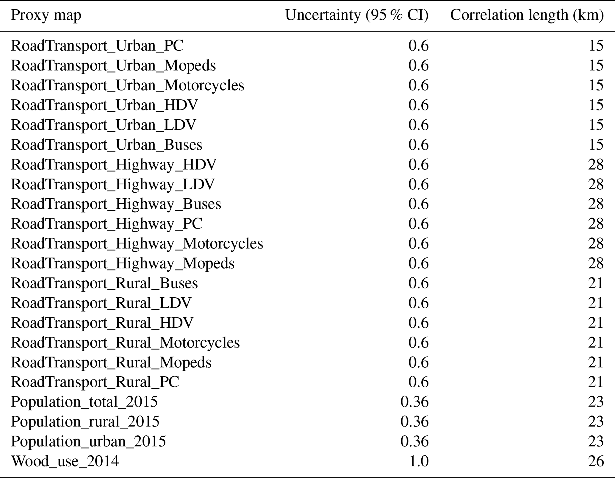
We include detailed spatial uncertainties for two GNFR sectors (road transport (GNFR F) and other stationary combustion (GNFR C)), which are the most important contributors to CO and CO₂ emissions from area sources and have the strongest CO:CO₂ error correlations. These sectors each consist of several sub-sectors that are downscaled with different proxy maps. By starting at the sub-sector level, each grid cell receives a unique uncertainty at the GNFR level, depending on the mix of sub-sectors. An overview of the proxy maps for these two GNFR sectors is given in Table 2. Note that spatial uncertainties are only included for countries for which emissions are downscaled using these proxies (and not for countries without reported emissions).

We start with the accuracy of the pixel value. The proxies for road transport are based on the Open Transport Map (Jedlička et al., 2016), which combines the OpenStreetMap (OSM) road network with traffic volume from traffic simulation models. OSM is community-based and is not always complete or accurate. Yet, the main source of uncertainty arises from the underlying traffic simulation models. A wide range of models exist, with each model having its own strengths and weaknesses. Some guidance on the accuracy of these models is given by Gao et al. (2010), who calculated an average RMSE of 31 % in traffic volume for two traffic models (MATSim and EMME/2). For another traffic model, VISUM, a similar mean relative error of 30 % was found (Raney et al., 2003). These studies therefore indicate a 95 % confidence interval (CI) of about 60 % (about 2 times the RMSE). However, both studies are performed at a very high resolution (street links), whereas our resolution is much coarser (∼ 6 km grid cells). Therefore, the uncertainty in our proxy map is probably smaller, and we set the 95 % CI to 30 %. The population density is based on LandScan (Bright et al., 2016). This product describes the ambient population, which includes both the working and travelling populations, by taking a 24 h average. Archila Bustos et al. (2020) compared LandScan to population data from the Swedish Statistics Bureau and found an average RMSE of 9 %, with larger errors observed for sparsely populated areas. This suggests that the uncertainty distribution is skewed, as also shown for Poland (Calka and Bielecka, 2019). Here, we assume that the RMSE is based on a sufficiently large population since the largest absolute errors occur in densely populated areas, and we estimate that the 95 % CI is more or less equal to 2 times the RMSE. Finally, the wood use proxy is based on population density and the proximity to wood/forests (Kuenen et al., 2022). The uncertainty is expected to be large as the locations where residential wood burning takes place are relatively unknown. For example, Grythe et al. (2019) demonstrated large differences in particulate matter emissions from residential wood combustion between different datasets, even when aggregated over large urban domains. We set the 95 % CI to 50 %.

Table 2 Overview of the proxy maps used for downscaling GNFR C (other stationary combustion) and GNFR F (road transport), including their 95 % CIs and correlation lengths. HDV: heavy-duty vehicle. PC: passenger car. LDV: light-duty vehicle.

The second source of uncertainty is the proxy quality, which is a difficult uncertainty with which to work. There is no way to correct a grid cell that falsely lacks activity as scaling a value of zero always returns zero. This is mainly an issue for categorical proxies, which are based on the presence of certain characteristics (e.g. land use types) rather than on numerical values. Similarly, if the location of a point source is incorrect, it is difficult to estimate where it should be instead. Since we cannot reliably compensate for this uncertainty, we have chosen not to account for it while acknowledging it as a local source of uncertainty in the location of emissions.

Finally, the representativeness error behaves differently from the uncertainty in the pixel values. Aside from adding uncertainty to each pixel, it also causes errors to be correlated between pixels that have similar characteristics. For example, the heating demand for residential buildings depends on population density. People who live closer together, e.g. in high-rise buildings, generally need less heating per person. This means that heating emissions are not linearly related to population. If we make an error in describing this relationship, it will affect pixels with similar characteristics in a similar fashion; hence, errors are spatially correlated. We double the pixel value uncertainty to include the representativeness error (Table 2). Moreover, we consider its impact on the error correlation, which is discussed in Sect. 2.2.1.

The other sectors receive a fixed uncertainty (95 % CI) for all grid cells, based on expert judgement. The public-power and industry sectors contain point sources, for which the locational error can be large (Hogue et al., 2016). However, for the TNO-GHGco-v4 emission inventory, locations have been thoroughly checked, and we assume no spatial uncertainty. The remainder (non-point sources) receives an uncertainty of 200 %. For sea shipping, the spatial patterns are relatively well known based on AIS data (Jukka-Pekka Jalkanen, personal communication, 15 September 2022), and we assume no spatial uncertainty. However, the AIS coverage for inland waterways is limited; therefore, we set the uncertainty at a level similar to that used for the road transport sector (60 %). The other sectors are minor but have a large spatial uncertainty. Since they are grouped, some errors may cancel each other out, and we assume an overall uncertainty of 200 %.

2.2 Prior emission uncertainties

In this section, we describe how the prior emission uncertainties were calculated. An overview of all the steps is given in Fig. 2. The details are described below.

Figure 2 Diagram of all the steps taken to calculate prior emission uncertainties and covariances.

2.2.1 Spatial error correlation length

The representativeness error in a proxy map causes errors to be spatially correlated. We define the error correlation length as the maximum distance at which two grid cells are still correlated. This length scale is estimated by fitting spherical and exponential semi-variograms to each proxy map listed in Table 2 for each country. A semi-variogram describes the spatial autocorrelation as a function of distance, i.e. the degree of variability between points located at a certain distance from each other. In the case of the proxy maps, points that are closer together are expected to be more similar, and, therefore, their errors are more strongly correlated. We use the “fit.variogram” function from the “gstat” geostatistical package in the R software (Pebesma and Wesseling, 1998) and take the range parameter as our length scale. We set the limits of the considered distance between 6 km (original grid spacing) and 120 km.

The fitting procedure optimizes the model parameters to provide the best fit to the data and shows only small differences between the spherical and exponential models. We perform this fitting procedure twice: once without setting an initial sill (the semi-variance at a distance of zero) and once with the initial sill set to zero. This is done to ensure that the resulting ranges are not just a consequence of the initial values set in the model. This results in two ranges per country per proxy map, and we pick the value that is within our set boundary or the average of the two values if both values are within this range. We can only use one correlation length for the entire domain to avoid irregularities near country borders; therefore, we take the median of all country-specific ranges. The results are illustrated in Sect. 3.1.

For the industry and public-power sectors, we set the error correlation length to zero since these sectors are dominated by point sources which have no spatial uncertainty. For shipping, we estimate an error correlation length of 100 km, which is larger than that for road transport, given that it is more difficult for ships to make a turn.

2.2.2 Error correlation between CO and CO₂ emissions

The proxy maps used for spatial downscaling are the same for all trace gases in the emission inventory; i.e. the CO₂ emissions of sub-sector X are downscaled with the same proxy map as that used for the CO emissions of sub-sector X. This means that, at the sub-sector level, the spatial errors are strongly correlated between all trace gases. Because the mix of sub-sectors within an aggregated sector can differ for CO compared to CO₂, the error correlation is reduced. Therefore, we define a predictor to estimate the error correlation between CO and CO₂ in each grid cell for other stationary combustion (GNFR C) and road transport (GNFR F). This predictor is validated against a Monte Carlo-based correlation coefficient for seven countries that reflect relevant variations in the domain (Czech Republic, Germany, France, UK, Italy, the Netherlands, and Sweden). This predictor is a measure of the dissimilarity between CO₂ and CO emissions within a grid cell and allows us to calculate the error correlation for all grid cells without having to perform an expensive Monte Carlo simulation.

The predictors (PC for GNFR C and PF for GNFR F), which are calculated per grid cell, are based on the CO and CO₂ emissions per grid cell (c) per proxy map (m) for the selected GNFR sector and the uncertainties (relative standard deviation (σ)) in the proxy maps. In Eq. (1), STD is the absolute standard deviation of the emissions per grid cell, proxy map, and trace gas. When the relative contribution of each proxy map differs strongly between CO and CO₂, the correlation is weaker, which is expressed in the weighted-difference (WD) vector (Eq. 2). The larger the number of proxy maps used for downscaling emissions from a particular sector, the stronger the correlation generally is. This is due to the damping effect on outliers. This results in the following set of equations:

$$\begin{array}{}\text{(1)}& {\displaystyle }\mathit{S}\mathit{T}{\mathit{D}}_{c,m,g}=f_{c,m}\cdot E_{m,g}\cdot {\mathit{\sigma }}_m,\text{(2)}& {\displaystyle }\mathit{W}{\mathit{D}}_{c,m}=\left|{\displaystyle \frac{\mathit{S}\mathit{T}{\mathit{D}}_{c,m,{\mathrm{CO}}_{\mathrm{2}}}}{\sum \left(\mathit{S}\mathit{T}{\mathit{D}}_{c,m,{\mathrm{CO}}_{\mathrm{2}}}\right)/n}}-{\displaystyle \frac{\mathit{S}\mathit{T}{\mathit{D}}_{c,m,\mathrm{CO}}}{\sum \left(\mathit{S}\mathit{T}{\mathit{D}}_{c,m,\mathrm{CO}}\right)/n}}\right|,\text{(3)}& {\displaystyle }{\mathrm{PC}}_c={\displaystyle \frac{\mathrm{stdev}\left(\mathit{W}{\mathit{D}}_{c,m}\right)}{n}}\text{ and }{\mathrm{PF}}_c={\displaystyle \frac{\max \left(\mathit{W}{\mathit{D}}_{c,m}\right)}{n}},\end{array}$$

where g is one of the two trace gases (CO or CO₂), f is the fraction of a proxy map in a grid cell, and n is the number of proxy maps contributing to a grid cell. Note that the predictor is slightly different for GNFR C and GNFR F, being based on the standard deviation and maximum value, respectively, of the WD values of the proxy maps contributing to each grid cell. We define a relationship between the predictor and the Monte Carlo-based correlation coefficient to calculate the CO:CO₂ error correlation per grid cell based on the predictor. For the Monte Carlo method, an ensemble of gridded emissions was produced by randomly perturbing the grid cell emissions of CO₂ and CO for each proxy map, following the defined uncertainty ranges. The perturbations are applied equally to CO₂ and CO emissions, assuming a full error correlation for each proxy map, which is a valid assumption at the grid cell level. The correlation coefficient results from a linear regression of the total CO₂ and CO emissions per grid cell for a given GNFR sector. The results are shown in Sect. 3.1 and the Supplement.

For the other sectors, we estimate a fixed value for all grid cells. For the public-power and shipping sectors, the correlation is likely to be very strong since there is little variation in sub-sector activities. Therefore, we set the error correlation to 0.95. For industry, the correlation is much smaller due to different sub-processes taking place, and we set the error correlation to 0.5.

2.2.3 Uncertainty propagation

We have now gathered all relevant information on the uncertainties, which needs to be propagated to match the level of detail pertaining to the dataset on prior emissions.

The country-level uncertainties represent a 95 % CI (normalized to be unitless), which is given either as one value or as lower and upper values. For the latter, when the lower and upper values show less than a 5 % difference, we use a Gaussian uncertainty distribution; otherwise, we use a log-normal uncertainty distribution. For CO, the uncertainty distribution is often log-normal. When the reported standard deviation exceeds 30 %, we also use a log-normal uncertainty distribution to avoid obtaining negative values. We use uncertainty propagation to estimate the uncertainty in emissions from the standard deviations (σ) in AD and EFs:

$$\begin{array}{}\text{(4)}& {\displaystyle \frac{{\mathit{\sigma }}_E}{E}}=\sqrt{{\left({\displaystyle \frac{{\mathit{\sigma }}_{\mathrm{AD}}}{\mathrm{AD}}}\right)}^{\mathrm{2}}+{\left({\displaystyle \frac{{\mathit{\sigma }}_{\mathrm{EF}}}{\mathrm{EF}}}\right)}^{\mathrm{2}}}.\end{array}$$

To examine the importance of error correlations in AD and EFs, we performed a sensitivity analysis on the European emissions (see the Supplement). We found that including error correlations in AD and EFs has limited importance, and, henceforth, we ignore these correlations.

Since these uncertainty error propagation equations assume Gaussian errors, we need to translate log-normal error distributions into equivalent Gaussian distributions. We approximate the Gaussian standard deviation of a log-normal distribution using

$$\begin{array}{}\text{(5)}& {\displaystyle \frac{{\mathit{\sigma }}_X}{X}}={\displaystyle \frac{(\ln \left({\lim }_{\mathrm{upper}}\right)-\ln \left({\lim }_{\mathrm{lower}}\right))}{\mathrm{4}}},\end{array}$$

where lim_upper is the 97.5 percentile and lim_lower is the 2.5 percentile of the log-normal distribution. Note that the combination of Gaussian and log-normal functions does not result in a log-normal function because the result can be negative. However, here we assume that the combined distribution is log-normal because the Gaussian uncertainty is often relatively small compared to the log-normal uncertainty.

The sub-sector-level emission uncertainty estimates are propagated to obtain an uncertainty estimate at the GNFR level:

$$\begin{array}{}\text{(6)}& {\mathit{\sigma }}_{E,\mathrm{agg}}=\sqrt{\sum _{i=s}^n{\mathit{\sigma }}_{E,\mathrm{sub},s}^{\mathrm{2}}},\end{array}$$

where the subscript “agg” refers to the aggregated emissions and uncertainties and the subscript “sub” refers to the sub-sectors that are part of the aggregated sector. To use Eq. (6), we need the emission budgets because this equation uses actual standard deviations instead of normalized ones.

These simple uncertainty propagation functions work well under specific circumstances. When uncertainties follow a non-Gaussian distribution or are correlated, a Monte Carlo simulation can provide a more reliable estimate of the final uncertainty. However, a Monte Carlo approach is also computationally demanding when using such an extensive dataset. We tested and compared both approaches for selected countries and sectors. Detailed information can be found in the Supplement, but the main conclusion is that we can mimic the results from the Monte Carlo simulation well with the uncertainty propagation functions. The methods show a similar order of magnitude and variability between countries and trace gases. Although there is no perfect match between the two methods, we argue that this source of uncertainty is negligible compared to the uncertainty in the prior uncertainty data.

For the spatial proxies, the same set of equations is applied, but to calculate the standard deviations, weighted proxy maps are computed. This means that for each combination of trace gas and country, we determine the relative contribution of each sub-sector to the GNFR sector, assign a weight to the corresponding proxy map, and multiply that value by the fraction in each grid cell. This also results in a new weighted-average proxy map for each GNFR sector, with a sum of 1 for each country. Next, we calculate the uncertainty in this weighted-average proxy map using Eq. (6), slightly adapting it so that the standard deviation is now related to the weighted fraction (Pw) per proxy map (m) in each grid cell. This results in

$$\begin{array}{}\text{(7)}& {\mathit{\sigma }}_{P,\mathrm{agg}}=\sqrt{\sum _{i=m}^n{\mathit{\sigma }}_{\mathrm{Pw},m}^{\mathrm{2}}}.\end{array}$$

The result of this is shown in Fig. 3.

Figure 3 Maps of gridded uncertainties (%) in CO₂ fossil fuel (ff) for the sectors corresponding to other stationary combustion (a) and road transport (b).

Finally, we determine the error correlation length for the GNFR sectors by calculating a weighted-average correlation length. However, because the combined correlation length is also slightly sensitive to the uncertainty in each proxy map, the larger the uncertainty, the more impact the spatial correlation has. Thus, we calculate the weight based on both the CO₂ emissions and the proxy map uncertainties (i.e. the relative emission share multiplied by the relative uncertainty share).

2.3 Inverse modelling approach

To examine the impact of the definition of prior uncertainties on multi-species inversion, we perform a series of closed-loop numerical experiments. For this, we generate a “true” emission and use a chemical transport model to determine the atmospheric concentrations of CO₂ and CO that would be observed by the in situ measurement network based on these true emissions (the true observations). We perform an inversion in which we confront a modelled atmosphere based on a prior estimate of emissions with “real” observations (true observations with noise), adjusting the prior estimate to minimize the model–observation differences. We can then compare the posterior and true emissions to determine whether our inversion approach is able to evaluate the accuracy of the prior estimate.

The analytical inversion approach is described elsewhere (e.g. Maasakkers et al., 2021), so we will only briefly describe it here. We use the model to generate a Jacobian matrix (K) that represents the observation sensitivity to emission perturbations. We then use the minimization of the Bayesian cost function to solve for the posterior scale factor (x^′),

$$\begin{array}{}\text{(8)}& {\mathit{x}}^{\prime }={\mathit{x}}^a+{\mathbf{S}}^a{\mathbf{K}}^{\mathrm{T}}{\left({\mathbf{KS}}^a{\mathbf{K}}^{\mathrm{T}}+\mathbf{R}\right)}^{-\mathrm{1}}\left(\mathit{y}-\mathbf{K}{\mathit{x}}^a\right),\end{array}$$

where x^a and S^a represent the prior scale factor and error covariance matrix, respectively, and y and R represent the observations and observing-system error covariance matrix, respectively. In the following sections, we describe the different aspects of the inversion system.

2.3.1 Atmospheric chemistry transport model

For the atmospheric chemistry transport model, we use version 12.5 of GEOS-Chem (The International GEOS-Chem User Community, 2019). We model CO₂ and CO concentrations over Europe (34–66° N, 15–35° E) for the year 2018. The model is run at a 0.25° × 0.3125° resolution and driven by Goddard Earth Observing System Forward Processing (GEOS-FP) meteorology from the NASA Global Modeling and Assimilation Office (Lucchesi, 2018). We use 3-hourly CO₂ and CO boundary conditions from a global simulation with GEOS-Chem at a 2° by 2.5° resolution. For anthropogenic CO₂ and CO emissions, we use the TNO-GHGco-v4 inventory, as described in Sect. 2.1.1, including sector-specific temporal scaling factors provided by TNO (Denier van der Gon et al., 2011), to increase the temporal resolution to a daily scale. We use fire emissions from version 4 of the GFED (Global Fire Emissions Database; van der Werf et al., 2017), biogenic fluxes from the vegetation model CASA-GFED (Ott, 2020), and ocean fluxes from Takahashi et al. (2009). For the inversion, we re-grid these emissions to basis functions (Fig. 4), which are created by aggregating regional emissions until a given emission threshold is reached while respecting country borders. We use pre-computed monthly 3-D fields of the hydroxyl radical sink of CO. Further details on the model setup are provided elsewhere (Palmer et al., 2022; Scarpelli et al., 2024). We assume a model uncertainty of 2 ppm and 8 ppb for CO₂ and CO, respectively.

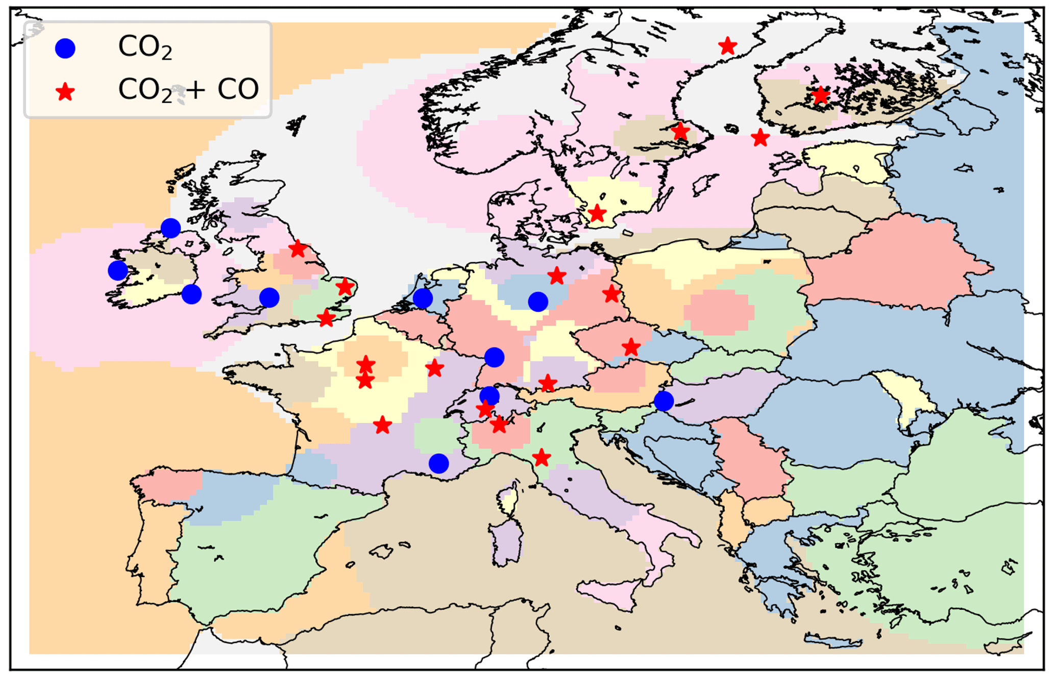
Figure 4 Map of the modelling domain, with the colours showing basis functions. The blue dots represent locations where CO₂ is measured, and the red stars represent locations where both CO₂ and CO are measured (Integrated Carbon Observing System, 2024).

2.3.2 State vector and error covariance matrix

The state vector consists of scale factors for the fossil fuel (${\mathit{x}}_{\mathrm{co}\mathrm{2}}^{\mathrm{FF}},{\mathit{x}}_{\mathrm{co}}^{\mathrm{FF}}$) and biogenic (${\mathit{x}}_{\mathrm{co}\mathrm{2}}^{\mathrm{Bio}}$) components, boundary conditions (${\mathit{x}}_{\mathrm{co}\mathrm{2}}^{\mathrm{BC}},{\mathit{x}}_{\mathrm{co}}^{\mathrm{BC}}$), and CO chemistry (${\mathit{x}}_{\mathrm{co}}^{\mathrm{Chem}}$) terms.

$$\begin{array}{}\text{(9)}& \mathit{x}=\left({\mathit{x}}_{\mathrm{co}\mathrm{2}}^{\mathrm{BC}},{\mathit{x}}_{\mathrm{co}}^{\mathrm{BC}},{\mathit{x}}_{\mathrm{co}}^{\mathrm{Chem}},{\mathit{x}}_{\mathrm{co}\mathrm{2}}^{\mathrm{Bio}},{\mathit{x}}_{\mathrm{co}\mathrm{2}}^{\mathrm{FF}},{\mathit{x}}_{\mathrm{co}}^{\mathrm{FF}}\right)\end{array}$$

These scale factors are optimized per basis function (Fig. 4) and per month. We assume prior Gaussian uncertainties of 50 %, 5 %, and 5 % for the biogenic components, boundary conditions, and CO chemistry scale factors, respectively.

For the fossil fuel state vector elements (${\mathit{x}}_{\mathrm{co}\mathrm{2}}^{\mathrm{FF}},{\mathit{x}}_{\mathrm{co}}^{\mathrm{FF}}$), we use a Monte Carlo approach to determine the prior uncertainties, taking advantage of the advanced uncertainty estimate presented here. Separate ensembles are made for the spatial distribution and the country-level emissions, which are combined into one ensemble of gridded emissions and fed into the inversion system.

First, we generate an error covariance matrix of country-level emissions, where each element corresponds to a single GNFR sector and species (CO₂ or CO). We use the standard deviations derived in Sect. 2.2.3 (σ_x) to populate the diagonal of the covariance matrix, whereas all off-diagonal values are set to zero (i.e. no error correlations).

Second, for a given GNFR sector, we generate an error covariance matrix for the spatial distribution using the uncertainties for the proxy maps described above. Each sector's error covariance matrix includes both CO and CO₂. The variances on the diagonal of the matrix are derived from the standard deviations described in Sect. 2.2.3 (and shown in Fig. 3). The off-diagonals of the error covariance matrix include the covariance between spatially neighbouring grid cells that belong to the same species (CO or CO₂), derived from the spatial error correlations described in Sect. 2.2.1, and the covariance between gridded CO and CO₂ emissions, derived from Sect. 2.2.2. For the error covariances within a single species, we define the covariances based on the spatial error correlation length l. For this, we define the exponential decay in the correlation coefficient r between elements i and j with distance d (Eq. 10). After distance l, we assume the correlation is zero, following Kunik et al. (2019).

$$\begin{array}{}\text{(10)}& r_{i,j}=e^{-d_{i,j}/l}\end{array}$$

We perform a Cholesky decomposition of each error covariance matrix, resulting in the matrix L. Combining this matrix with a vector of uncorrelated random samples (u) from a Gaussian distribution, where μ = 0 and σ=1, through a dot product gives us a perturbation vector (p) that has the covariance properties of the entire system. We can do this for m unique perturbation vectors to generate an ensemble of m spatial distributions or country-level emissions (x_m) as follows:

$$\begin{array}{}\text{(11)}& {\displaystyle }{\mathit{p}}_m=\mathbf{L}\cdot {\mathit{u}}_m,\text{(12)}& {\displaystyle }{x}_m=\overline{x}{p}_m+\overline{x},\end{array}$$

where x_m represents the estimated values of the spatial map for a given sector (including CO₂ and CO) with respect to ensemble member m and $\overline{x}$ is the expected value of the spatial distribution.

Alternatively, for variables with a log-normal distribution, we calculate the ensemble values using

$$\begin{array}{}\text{(13)}& x_m=\overline{x}{e}^{{\mathit{p}}_m}.\end{array}$$

The ensemble of gridded emissions is a combination of the ensemble of spatial distributions and country-level emissions.

2.3.3 Observations

We generate true emissions by perturbing the inventories of prior emissions based on assumed error statistics, as described previously, assuming that the previously described error correlation between CO₂ and CO is true. For the true observations, we sample the 3-D modelled concentration fields observed by the Integrated Carbon Observation System (ICOS) in situ network (Fig. 4), and, because our system is linear, we can apply the same perturbations to the observation vectors as those applied to the true emissions. The true observations are the CO₂ and CO concentrations that would result from the occurrence of the true emissions. We generate our real observations by adding a noise term to the true observations, simulating what the observing network would have generated had the true emissions occurred. The noise term is a vector of perturbations taken from a Gaussian distribution with a mean of 1 and standard deviations of 2 ppm and 4 ppb for CO₂ and CO, respectively, and represents the observation uncertainty (i.e. the instrumentation error and the uncertainty in the comparison of the gridded model output with point observations). The observations are 3-hourly averages (between 09:00 and 18:00 LT), aligning with the temporal resolution of the model's meteorology.

2.3.4 Experiments

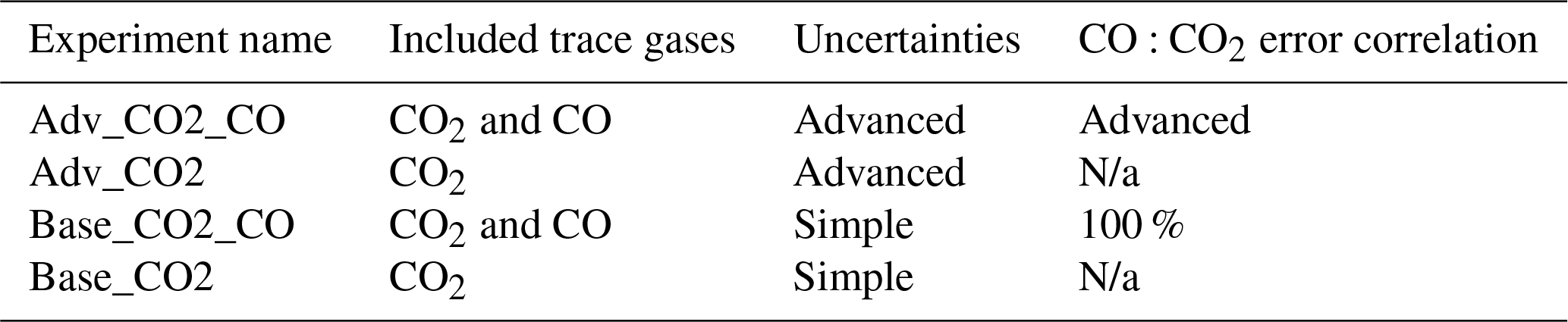
To illustrate the impact of the new definition of prior uncertainties, we also report the results from a second inversion approach, which assumes a 100 % error correlation between CO₂ and CO emissions from fossil fuel combustion, allowing for the use of one shared fossil fuel scale factor for both CO₂ and CO (x^FF). This uncertainty definition has been used before by Palmer et al. (2022) and serves as a base experiment. Assuming a 100 % error correlation is not very realistic, and with the numerical experiments, we test whether adjusting the CO₂ and CO error statistics to be closer to the “truth” would provide a benefit over the base scenario. For the base scenario, we use a combustion uncertainty of 10 % for the entire domain and a spatial error correlation length of 20 km. For comparison, the mean prior uncertainty in the advanced experiment is 7.7 % for CO₂ and 11.8 % for CO. Finally, we perform the same numerical experiments without CO.

Table 3 Overview of inversion experiments. The advanced uncertainties and CO:CO₂ error correlations refer to those developed here. Simple uncertainties refer to a fixed 10 % combustion uncertainty. These are combined with a full CO:CO₂ error correlation; i.e. one scaling factor applies to both CO₂ and CO fossil fuel fluxes. N/a: not applicable.

3 Results

3.1 Assessment of prior uncertainties and error correlations

First, we show the results from the prior uncertainty calculations before reporting the results from the closed-loop numerical experiments. The spatial error correlation lengths calculated per proxy map per country are shown in Fig. 5, including the median value for all countries. The resulting correlation lengths are also given in Table 2.

Figure 5 Derived correlation lengths for (a) a European proxy map of total population density and (b–d) road transport proxy maps, categorized by road type, for all vehicle types combined, binned in 5 km increments. The dashed black line shows the median value.

For population density, there are large differences between country groups – for example, between northern and southern Europe and between eastern and western Europe. The clustering of people in cities and rural areas within these broad geographical regions differs on a regional basis and affects the correlation lengths accordingly. Nevertheless, the largest group of countries shows correlation lengths of less than 30 km, which, given the resolution of the data assimilation system, is relatively small (∼ 5 pixels). For wood use, which we use as a proxy map for residential biomass combustion, we see a large cluster around 20–30 km (not shown), and there are only a few countries with significantly different length scales. For the road transport proxy maps, the various vehicle types (passenger cars, light-duty vehicles, and heavy-duty vehicles) do not show much variability in correlation length, but differences are evident for different road types; consequently, we combine the vehicle types to obtain road transport correlation lengths per road type. This results in longer length scales for highways than for urban roads. In urban areas, short distances are covered more frequently, resulting in weaker correlations in road transport activity between locations.

Next, we predict the CO:CO₂ error correlation that results from the shared activity between the trace gases. The relationship between the Monte Carlo-based CO:CO₂ error correlations and the predictor (Eq. 3) is shown in Fig. 6. As mentioned before, the Monte Carlo simulation is performed for seven selected countries. We find a clear cosine-shaped relation for GNFR C (other stationary combustion), allowing the correlation coefficient to be estimated with the following equation:

$$\begin{array}{}\text{(14)}& r=a\cdot \cos (b\cdot {\mathrm{PC}}_c),\end{array}$$

where a and b are parameters estimated from the fit shown in Fig. 6. The a parameter denotes the highest possible correlation coefficient, which, for pixels with emissions from only one sub-sector, should have a value of (close to) 1. For the seven individual countries, the a parameter lies between 0.96 and 1.03. Since a correlation coefficient of more than 1 is not possible, we set the a parameter to a maximum of 1. The b parameter is the period of the cosine function, which indicates how sharply the function declines with increasing predictor values. This parameter is between 3.36 and 4.44 for these seven countries. The mean for all countries is 3.60.

We see some grid cells with a predictor value of zero, whereas the correlation coefficient is much lower than the a parameter. In these cases, there are only two proxy maps with the same shares for CO and CO₂ (hence, a stdev(WD) value of zero is used in Eq. 3). These cases mostly occur in Sweden, resulting in a relatively poor fit of the cosine function (R² of 0.46). Overall, these cases make up 0.1 % of all grid cells, and they have no significant impact on the definition of the average function, which has an R² value of 0.85. The fit for the other individual countries ranges between 0.79 and 0.98. Plots for individual countries are shown in Fig. S3 in the Supplement.

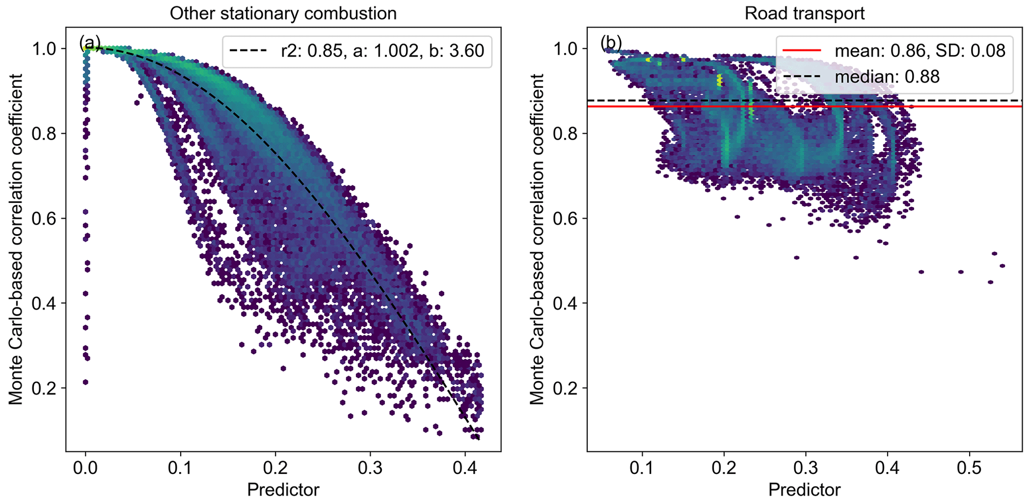
Figure 6 Hexbin plots of Monte Carlo-based (N=500) correlation coefficients (r) per grid cell against the predictor calculated using Eq. (3). In panel (a), the fit (R²) and cosine function parameters are shown. In panel (b), the mean, median, and standard deviation (SD) of the correlation coefficients are shown.

For road transport, it is more difficult to extract a relationship between the predictor and the correlation coefficient. For individual countries, we mostly see several cosine-shaped structures (shown in Fig. S4 in the Supplement), which makes it impossible to identify one single function. To understand this behaviour, we looked in more detail at the vehicle and road types. Although different vehicle types show very similar cosine functions within a country (Fig. 7), when we combine them, the structure disappears. The relationship between the predictor and the correlation coefficient seems to depend not only on the vehicle type but also on the number of road types present in a grid cell. When combining all road and vehicle types, they start to affect each other, meaning within the scatter plots, we can no longer identify the vehicle types. Because we do not separate vehicle and road types in our prior uncertainty data for the data assimilation system, we only want one value. Compared to the sector corresponding to other stationary combustion, we see much less variability in the correlations; therefore, we use the median value of 0.88. For individual countries, the median value lies between 0.82 and 0.96.

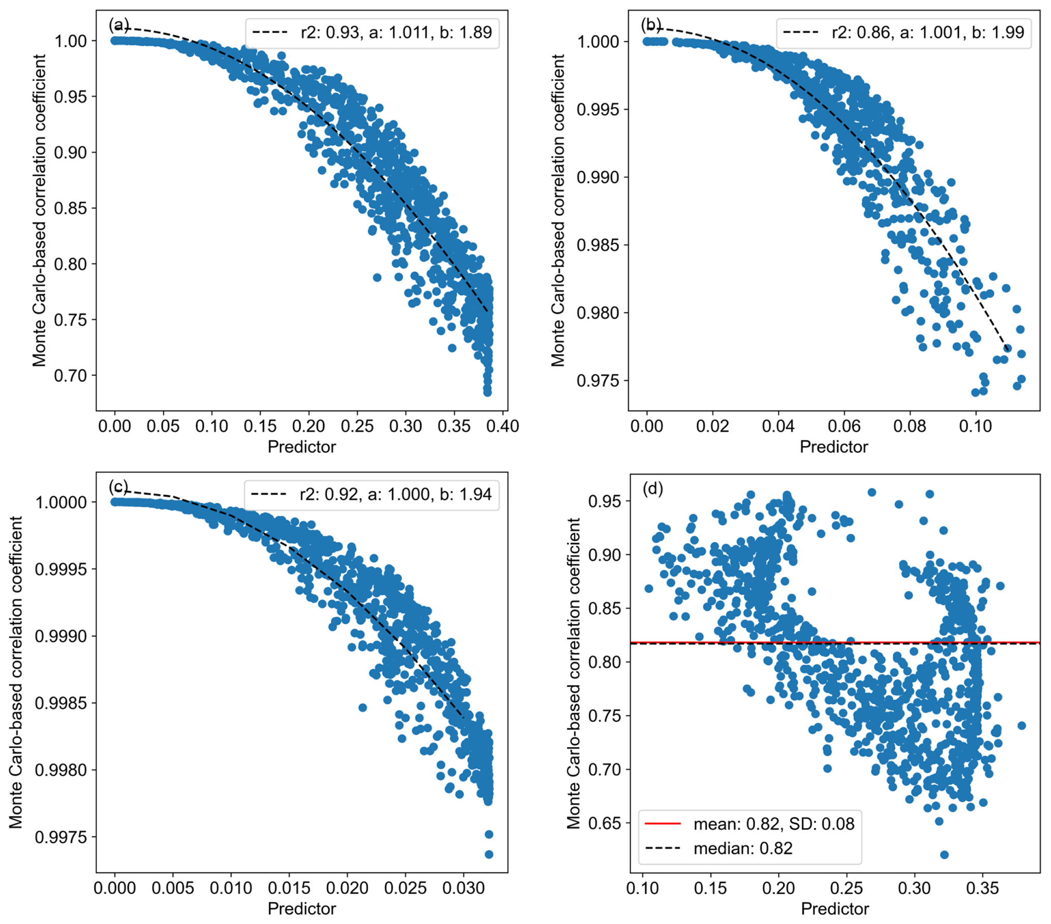
Figure 7 Scatter plots of Monte Carlo-based (N=500) correlation coefficients (r) per grid cell are presented against the predictor calculated using Eq. (3) for the Netherlands with respect to road transport per vehicle type (PC: passenger car; LDV: light-duty vehicle; HDV: heavy-duty vehicle). The correlation (R²) and cosine function parameters per vehicle type are also shown. Note that the range of values for LDV and HDV vehicles is very small compared to that for PCs (different y axis). Panel (d) shows the same scatter plot with all vehicle types combined, including the mean, median, and standard deviation (SD) of the correlation coefficients.

3.2 The effect of the definition of prior uncertainties

Next, we examine the impact of including this advanced definition of gridded emission uncertainties and error covariances on our ability to estimate CO₂ combustion emissions in an inversion framework. Figure 8 shows the annual average difference between the absolute prior and posterior deviations from the true emissions: $\left|\frac{\sum \left(E_{\text{prior,monthly}}-E_{\text{true,monthly}}\right)}{\mathrm{12}}\right|-\left|\frac{\sum \left(E_{\text{posterior,monthly}}-E_{\text{true,monthly}}\right)}{\mathrm{12}}\right|$. Positive (negative) values, represented by red (blue) colours, indicate that the posterior is closer to (further from) the truth than the prior. With the base uncertainties, there are several areas in which the results deteriorate (blue colours), such as the Netherlands, the southeast of the UK, and some locations in Germany. The differences range from −4.59 to 10.87 and from −5.13 to 11.99 kg s⁻¹ for the Base_CO2 and Base_CO2_CO experiments (Table 3), respectively. When using the advanced uncertainties, these blue colours start to disappear, and the differences range from −2.58 to 12.31 and from −1.60 to 12.92 kg s⁻¹ for the Adv_CO2 and Adv_CO2_CO experiments, respectively. The average CO₂ fossil fuel flux in this domain has a value of 7.55 kg s⁻¹, with a maximum value of just over 2000 kg s⁻¹. With the default uncertainties, the maximum deviation of fossil fuel CO₂ from the prescribed truth is about 7 % for both the prior and posterior results. With the advanced uncertainties, this is reduced to 4 % and 3 % in the posterior for the experiments without and with CO, respectively. Hence, the relative differences are small but still show a consistent improvement with the advanced uncertainties.

Figure 8 Maps of prior–posterior annual average absolute deviations from the truth in fossil fuel CO₂ emissions for all four experiments. Units are given in kg s⁻¹ per grid cell. Note that the bounds of the colour bars are set from −2.5 to 2.5 kg s⁻¹.

Generally, there seems to be fewer areas with significant deviations from the prior when using the advanced uncertainties, and regions that still show differences in the experiments with advanced uncertainties mostly show an improvement. The number of grid cells in Fig. 8 with values of more than 1 or less than −1 corresponds to 52, 80, 40, and 32 for the respective panels. The share of these grid cells with deteriorated results (blue colours) is 39 %, 50 %, 8 %, and 6 % for the respective panels. This suggests that with the advanced uncertainties, the system has a greater ability to constrain fossil fuel CO₂ emissions. This is also illustrated by the reduced posterior error correlation between the CO₂ biogenic and fossil fuel fluxes (Fig. 9). Although the differences are not significant, we see a tendency for more areas with near-zero correlations when using the advanced uncertainties. Note that the prior error correlations between biogenic and fossil fuel CO₂ fluxes have a value of zero. A high posterior error correlation means that the inversion system is unable to assign model–data mismatches to specific sources and instead updates multiple scaling factors at once, which has a lower cost. For individual months, we see a tendency for small negative error correlations in winter months and a tendency for somewhat larger positive error correlations in summer months for the Adv_CO2_CO experiment, which indicates that CO might be a better constraint for CO₂ fossil fuel fluxes during winter. This likely has to do with the large biogenic fluxes during summer, whereas CO emissions are lower during this period. However, based on only 1 year of monthly averages, we cannot draw any definite conclusions on this.

Figure 9 Histograms showing posterior error correlations between CO₂ biogenic (bio) fluxes and CO₂ ff fluxes for all basis functions across all four experiments. Mean values are indicated by a vertical red line.

3.3 Combining CO and CO₂

Figure 8 also shows that adding CO to the experiment with the base uncertainties causes more areas to show significant differences between the prior and posterior. Moreover, on average, the deviations from the prior are larger as well. Since the main source of CO is fossil fuel combustion and the uncertainties in CO emissions are large, this pollutant is more sensitive to errors in prior emissions and, therefore, causes larger deviations from the prior. This indicates that CO adds additional information on fossil fuel fluxes to the system, which causes the model–data mismatch in CO₂ to be assigned more clearly to either the CO₂ biogenic fluxes or the fossil fuel fluxes. This is also illustrated in Fig. 9, which shows the posterior error correlations between CO₂ biogenic and fossil fuel fluxes. When adding CO to the base experiment, the mean correlation per basis function is closer to zero. This also results in a slight improvement in the posterior scaling factors for CO₂ biogenic fluxes (Fig. 10). The results of the advanced experiments are not significantly different from those of the base experiments because most of the information from the observations has already been used to update the biogenic fluxes due to their high uncertainty.

Figure 10 Scatter plots of true vs. posterior scaling factors for CO₂ biogenic (bio) fluxes in the base experiment without CO and in the base experiment with CO, with the dashed line representing the 1:1 line. The posterior (Post) correlation coefficient (R²) and standard deviation are also given.

However, Fig. 8 shows more blue colours for the Base_CO2_CO experiment than for the Base_CO2 experiment, e.g. in northern Italy, which means that the results for CO₂ fossil fuel fluxes are actually worse than when only using CO₂. The number of grid cells with blue colours increases from 39 % to 50 %, as discussed before. This pattern is not visible when comparing the Adv_CO2 and Adv_CO2_CO experiments. For the Adv_CO2_CO experiment, the share of grid cells with blue colours is even slightly smaller than that for the Adv_CO2 experiment (8 % vs. 6 %). In other words, adding CO can deteriorate the results from experiments in which the prior error correlation is not correctly defined due to the sensitivity of CO to assumed prior emission uncertainties. Using a full CO:CO₂ error correlation causes larger changes in the scaling of CO₂ fossil fuel fluxes because the uncertainties in CO are relatively large and can be scaled easily. CO₂ then follows suit, which is clearly not always correct. With the advanced uncertainties, there are fewer large changes when comparing the experiments with and without CO. However, there are some small improvements visible in the UK, and results show no spurious changes in CO₂. Hence, in the combined optimization of CO₂ and CO, there is a clear need for advanced uncertainties to prevent inaccurate emission corrections.

4 Discussion and conclusions

We presented here a detailed assessment of prior emission uncertainties to support data assimilation studies. Prior uncertainties have a significant impact on data assimilation as they determine the extent to which prior emissions can be corrected. Underestimating the uncertainties limits the freedom of the system with respect to correcting the prior, which means that the actual state can be outside the uncertainty range and therefore unreachable. Overestimating the uncertainties reduces the constraint pertaining to the prior information, meaning that we do not make optimal use of the prior knowledge provided to the system. Moreover, a definition of prior uncertainties that includes covariances enables us to use co-emitted species to estimate fossil fuel CO₂. Hence, a realistic definition of prior uncertainties is important.

Building on the work of Super et al. (2020a), we developed a definition of prior uncertainties that is based on the uncertainties in the underlying data used to create the emission inventory. This ensures that the uncertainty definition is fully consistent with the emissions and consistent across multiple species (here, CO₂ and CO). We presented a more detailed analysis of the spatial uncertainties, including a description of spatial error correlation lengths. We particularly focused on CO₂:CO error correlations, which are caused by shared activities that result in emissions and mainly manifest in spatial patterns.

An important source of uncertainty in this work is the detailed uncertainty data that we use as a starting point, i.e. the reported emission uncertainties and the uncertainties in the spatial proxies. For GHGs, the reported country-level uncertainties are used. The IPCC not only encourages countries to make country-specific uncertainty assessments based on expert judgement but also provides default options (Eggleston et al., 2006). Therefore, the reported uncertainties are not necessarily consistent between countries. Nevertheless, we adopt these reported uncertainties to ensure our uncertainty estimates are well documented and consistent in terms of methodology. For spatial proxies, uncertainties are also based partly on expert judgement in the absence of better quantification. For the representativeness error, we assume a similar order of magnitude as the proxy value uncertainty, which is an arbitrary choice. Hogue et al. (2016) estimated the uncertainty of using population density as a proxy for CO₂ emissions by comparing differences in emissions per capita across all US states. They found that the representativeness error is often the dominant source of uncertainty; hence, we argue that our estimate is conservative to be on the safe side when estimating the impact of adding CO and improving the prior uncertainty estimate in our experiments. Since we start with a high level of detail, we assume a certain fraction of the random errors in the prior uncertainty information will cancel out. Moreover, we ignore the proxy quality as a source of uncertainty. We evaluate our approach by comparing the results against previous work. The country-level and grid cell uncertainties differ only slightly from the results of Super et al. (2020a). These results are discussed in detail there, whereas here we only focus on the spatial error correlation lengths and CO₂:CO error correlations. We evaluate the overall definition of prior uncertainties using closed-loop numerical experiments, which we discuss below.

The spatial error correlation lengths have been estimated by fitting semi-variograms to the proxy data and range between 15 and 28 km, which is about 2.5–4.5 times the grid size. Kunik et al. (2019) used a similar approach to estimate the length at which the difference between two emission inventories was still correlated. They found a correlation length scale of 6 km, which is about 6 times the grid size. Other studies optimized the correlation length based on the spatial scale and resolution of their inversion and the density of the observation network. Generally, a larger spatial-correlation length means a larger aggregated uncertainty, and, therefore, a larger correction to the observations is possible. Hence, this length scale can be optimized statistically. For example, Lauvaux et al. (2016) examined the impact of the spatial-correlation length on inversions to estimate CO₂ fluxes from the city of Indianapolis in the US. They found that ignoring the spatial correlation resulted only in local emission adjustments around the measurement sites because areas further from these sites are not constrained by the observations. Increasing the correlation length to 12 km adjusts the emissions for the entire city at once, and the spatial patterns are not affected. They concluded that a correlation length of 4–5 km is most suitable for making optimal use of the observations and prior information (Nathan et al., 2018). Similar conclusions were drawn for N₂O on a European scale (Corazza et al., 2011) and for biogenic CO₂ fluxes (Lauvaux et al., 2012). Of course, the optimal length scale based on this approach depends strongly on the spatial scale considered, and we consider our correlation lengths to be relatively low compared to the observation network. Based on these findings, we argue that it is necessary to combine the data-driven estimate with a statistical approach to find an optimal correlation length. Unfortunately, a methodology for this is not yet existent. Moreover, the spatial-correlation length scale may depend on the considered timescales (Carouge et al., 2010). Hence, more work is needed on this topic.

We developed a new approach to define the CO:CO₂ error correlation. Previous studies have often assumed a perfect correlation between the errors in CO₂ and CO fossil fuel fluxes, e.g. through a fixed emission ratio (Brioude et al., 2013; Nathan et al., 2018). However, emission ratios have a large uncertainty, and, therefore, the CO₂ and CO errors are not perfectly correlated. Only few studies have tried to estimate the inter-species error correlation or have performed sensitivity tests. Palmer et al. (2006) tried to make use of the synergy between CO and CO₂ by calculating error correlations per country. These correlations are very small because the CO EF dominates the uncertainty but is uncorrelated with CO₂. They concluded that the error correlation should be larger than 0.5 for CO to be a useful constraint for CO₂ fluxes, which is unrealistic at the country level. However, for gridded emissions, the correlation is much stronger as spatial patterns are linked to the activity. Moreover, the correlation is larger for individual sectors. Therefore, we argue that our calculated grid cell correlations, which range from 0.18 to 0.99 (with a mean value of 0.89), are realistic, considering that they are sector-specific and gridded. Additionally, Boschetti et al. (2018) tested different correlation strengths (0.1–0.9) and found no significant difference in the posterior fluxes, although uncertainty reduction increased with stronger correlations. This makes sense because it means more information is taken from CO priors and observations. We also find larger uncertainty reductions when we add CO to the base case – i.e. when there is a CO:CO₂ error correlation of 1. However, we also illustrate that the results do not always improve. The reason could be that Boschetti et al. (2018) assumed one error correlation value for the entire domain and also evaluated their results across the entire domain. Given the ranges in the prior–posterior absolute uncertainties shown in Fig. 8 for the Base_CO2 and Base_CO2_CO experiments, we also see no significant difference in the domain's total emissions. However, we do see clear differences across regions.

Closed-loop numerical experiments are useful for evaluating the capability of observing systems, including assumed prior and measurement error covariance matrices, to determine accurate estimates of carbon fluxes (Masutani et al., 2010). However, they also have limitations. The theoretical impact of an observing system will depend on several factors, including the quality of the atmospheric transport model used, the assumed structure and values used by the assimilation error covariance matrices, and the spatial distribution of the observations. Some of these choices can be based on expert judgement. For our numerical experiments, we are also limited by the resolution of our basis functions, and it is likely that we would see greater benefits from the Adv_CO2_CO experiment if the inversion were performed at a high resolution, leveraging the fine-scale variability in the error correlations between CO and CO₂ (e.g. along road networks).

Our numerical experiments illustrate the impact of the prior emission uncertainties. From these experiments, we can draw two important conclusions: (1) the definition of prior uncertainties is important for differentiating between different fluxes, such as biogenic and fossil fuel CO₂, and (2) CO can provide an additional constraint for estimating fossil fuel CO₂ fluxes only if the error covariance structure is defined realistically. Generally, it is difficult to constrain CO₂ fossil fuel flux estimates due to the high uncertainty in biogenic fluxes. However, we show here that, with the improved uncertainty definition, the posterior error correlation between biogenic and fossil fuel CO₂ is weaker. A likely explanation for this is that the largest fossil fuel sources are often clustered in areas that differ from those with the largest biogenic fluxes. Hence, when describing the spatial error structure correctly, the estimation framework used within the numerical experiments can more easily detect which source is dominant and update the estimates accordingly. Additionally, we have shown that CO provides additional information on the CO₂ fossil fuel fluxes in the base experiments, whereas it has a minor impact on the experiments with the updated prior uncertainties. Since CO has relatively large prior uncertainties (in emissions, models, and observations) compared to CO₂, the prior and observational information of CO contributes little weight to the cost function. By setting the CO:CO₂ error correlation to 1, the CO information becomes more important and thus results in larger corrections. The CO:CO₂ error correlations in the advanced experiment are relatively high (e.g. 0.88 for road transport), so this is likely not the only reason. It is likely that a better definition of the prior uncertainties will help to weigh all the information more effectively and, therefore, address some of the spurious changes seen in the Base_CO2_CO experiment.

In this study, we have used synthetic in situ observations obtained across the UK and mainland Europe, which have limited spatial coverage, with only 29 stations measuring CO₂, of which 19 also measure CO. Additionally, these stations are located in remote areas with limited local influence, and, therefore, they are not very sensitive to fossil fuel fluxes. Figure 8 shows that fluxes are mostly altered in central Europe, where the observation network is densest; therefore, enough information is available to update the data on prior emissions. Moreover, in these regions, the fossil fuel fluxes are the largest. This stresses the need for a wide observation network, ideally with co-located observations of CO₂ and co-emitted species, located in or near areas with high fossil fuel fluxes. For this reason, we also argue that the added value of CO is likely more pronounced with satellite data. The CO₂ column observed by satellites has limited sensitivity to CO₂ emissions perturbations, so our ability to constrain fossil fuel CO₂ fluxes separately from biogenic fluxes is limited. For the co-emitted species, i.e. CO and NO₂, the atmospheric column has a higher sensitivity to perturbations of combustion emissions, adding value to their inclusion in the inversion (Konovalov et al., 2016; Liu et al., 2020; Nathan et al., 2018; Reuter et al., 2019). In addition, satellite instruments like the TROPOspheric Monitoring Instrument (TROPOMI) provide high-density observations of CO and NO₂ globally, increasing the information content of the inversion compared to a CO₂-only inversion, whereas for the in situ network used here, we have fewer in situ stations with CO observations compared to those measuring CO₂.

Finally, our work illustrates the importance of using an accurate definition of prior uncertainties in CO₂ inversion and multi-species inversion. A concerted effort is needed to quantify the prior uncertainties in a way that is consistent with the data and optimized for application in data assimilation studies. There is much room for further improvement in current work – for example, by adding more detailed uncertainty estimates for sectors other than road transport and other stationary combustion. Given the nature of the spatial proxy maps for the other sectors, which are often categorial or contain point source locations, this poses an additional challenge. Furthermore, temporal uncertainties need to be added as they can have a major impact on data assimilation results (Super et al., 2021).