the Creative Commons Attribution 4.0 License.
the Creative Commons Attribution 4.0 License.
 | 19 Aug 2024
Objective identification of meteorological fronts and climatologies from ERA-Interim and ERA5
Philip G. Sansom
Jennifer L. Catto
Meteorological fronts are important due to their associated surface impacts, including extreme precipitation and extreme winds. Objective identification of fronts is therefore of interest in both operational weather prediction and research settings. The aim of this study is to produce a front identification algorithm based on earlier studies that is portable and scalable to different resolution datasets. We have made a number of changes to an earlier objective front identification algorithm, applied these to reanalysis datasets, and present the improvements associated with these changes. First, we show that a change in the order of operations yields smoother fronts with fewer breaks. Next, we propose the selection of the front identification thresholds in terms of climatological quantiles of the threshold fields. This allows for comparison between datasets of differing resolutions. Finally, we include a number of numerical improvements in the implementation of the algorithm and better handling of short fronts, which yield further benefits in the smoothness and number of breaks. This updated version of the algorithm has been made fully portable and scalable to different datasets in order to enable future climatological studies of fronts and their impacts.
- Article
(16448 KB) - Full-text XML
-
Supplement
(10464 KB) - BibTeX
- EndNote


Atmospheric fronts are of great importance for the day-to-day variability in weather in the mid-latitudes. They are associated with a large proportion of both total and extreme precipitation, as demonstrated by case studies (Browning, 2004); modelling (Browning, 1986; Sinclair and Keyser, 2015); and, more recently, long-term climatologies (Berry et al., 2011b; Parfitt et al., 2017b; Schemm et al., 2017). They are also strongly linked to extreme wind events (Dowdy and Catto, 2017; Catto et al., 2019; Raveh-Rubin and Catto, 2019; Catto and Dowdy, 2021) and are key to air–sea interaction (Parfitt et al., 2017b). With a wealth of global gridded observationally constrained and model-produced data, there is a desire to be able to objectively identify these frontal features in the gridded data. This avoids the huge time requirements of a manual analysis and allows for the features to be linked to high-impact weather, such as extreme precipitation or winds (Catto et al., 2012; Catto and Pfahl, 2013; Dowdy and Catto, 2017). The application of the methods to model data of historical and future climate also allows for the models to be evaluated on their ability to capture the dynamical features and their connection to precipitation events (Leung et al., 2022) and to investigate the future of such features and how they may impact water resources and natural hazards (Catto et al., 2014).
A number of methods have been developed to perform such objective identification. Hewson (1998, referred to hereafter as H98) compiled a summary of methods used to identify frontal features in gridded data and further developed the methods based on a thermal front parameter. Thomas and Schultz (2019) highlighted the three main factors required in identifying fronts with such a thermal front parameter: first, the thermal variable and vertical level to be considered, e.g. temperature, potential temperature, or equivalent (or wet-bulb) potential temperature at 850 hPa; second, a function of the variable, e.g. the gradient or some second or third derivative; and, finally, some thresholds. They found that different thermal variables each had pros and cons and could be selected depending on the purpose of the study. The study by Jenkner et al. (2010) used equivalent potential temperature and its second derivative to place the frontal lines. This results in the fronts lying in the centre of a frontal zone rather than at the leading edge, as a synoptic meteorologist would typically put them. Berry et al. (2011b) directly applied the methods of H98 to gridded data at 2.5°×2.5° resolution, placing fronts on the warm side of the strong temperature gradient. This also included the addition of a numerical line-joining algorithm, which is used to link the frontal points to line features.
Other methods have used dynamical information to identify fronts. Simmonds et al. (2012) used information solely on wind shifts. This method was found to work better in the Southern Hemisphere than the Northern Hemisphere by Schemm et al. (2015). A combination of this and the thermal method was used by Bitsa et al. (2021) to identify cold fronts in the Mediterranean, with the method tailored to suit the smaller spatial scale of fronts in this region. Parfitt et al. (2017b) used a combination of vorticity and temperature, requiring both a thermal gradient and a wind shift. While each method has its advantages and disadvantages, many of the methods typically identify many of the same features (Hope et al., 2014).
A major difficulty in applying objective front identification is the many datasets and differing resolutions. This is particularly an issue when using gradients of thermal properties since the resolution of the data will have a large impact on these gradients. The thresholds used to define fronts need to be varied depending on the resolution. Recently, Soster and Parfitt (2022) investigated the sensitivity of results to the use of different datasets and found a large difference in front frequency between the datasets. Higher-resolution datasets consistently show higher frequency of frontal points, with the differences reduced when re-gridded to a common grid. This was shown to lead to large differences between datasets in the proportion of precipitation attributed to fronts.
Despite the many methods of identifying fronts and issues and uncertainties associated with each of them, the thermal front parameter method of H98 has been successful in identifying the key climatological features of front frequency and the link to other variables in a number of studies (e.g. Berry et al., 2011a, b; Catto et al., 2012, 2014; Catto and Pfahl, 2013; Dowdy and Catto, 2017). Those studies used either the ERA-40 reanalysis of the European Centre for Medium-Range Weather Forecasts (ECMWF) (Uppala et al., 2005) at 2.5°×2.5° resolution or, later, the ECMWF ERA-Interim (Dee et al., 2011) reanalysis at 0.75°×0.75° resolution. However, the code used in those studies was not easily portable due to it being written in a mixture of the National Center for Atmospheric Research (NCAR) Command Language (NCL, 2011) and FORTRAN 77 (1978) and did not easily scale to the ECMWF ERA5 reanalysis at 0.25°×0.25° or other high-resolution datasets. The aim of this study is to create a portable implementation of the front identification method of H98 that is able to scale to contemporary high-resolution (re)analyses with horizontal grid spacings of 0.25° or less. We demonstrate a quantile-based method of tuning the thresholds. First, the data used are described in Sect. 2. Section 3 gives a description of the thermal front parameter method and the improvements over the previous implementation of the algorithm. In Sect. 4, we compare the front climatology using the new method with previous methods and different datasets. We finish in Sect. 5 with a discussion of the benefits and challenges associated with such objective identification methods.
The updated front identification procedure is applied to the ECMWF ERA-Interim reanalysis (ECMWF reanalysis – Interim; Dee et al., 2011). The data used here have a resolution of 0.75°×0.75° on a regular longitude–latitude grid. The 6-hourly instantaneous air temperature and specific humidity fields at the 850 hPa level were used to compute the wet-bulb potential temperature, θW, using the direct method of Davies-Jones (2008, Eq. 3.8), in order to identify fronts. The 6-hourly eastward and northward wind components at 850 hPa were used to compute the front speed using Eq. (13) of H98, allowing for classification into cold, warm, or quasi-stationary fronts. ERA-Interim was chosen over the more recent ERA5 reanalysis (ECMWF reanalysis v5; Hersbach et al., 2020) for the primary analysis since the updated procedure is of greatest benefit in middle- and low-resolution models and the resolution of ERA-Interim is equal to that of the highest resolution among standard CMIP6 general circulation models (GCMs). Our baseline for comparison is the global climatology of fronts in ERA-Interim at 0.75°×0.75°, produced by Dowdy and Catto (2017) using the method of Berry et al. (2011b). We also present a high-resolution climatology based on applying the updated front identification procedure to the ERA5 reanalysis using the same 6-hourly fields as ERA-Interim but with a grid spacing of 0.25°×0.25°.
Following H98 and Berry et al. (2011b), fronts are identified in the wet-bulb potential temperature field, θW, at 850 hPa. As described in H98 (their Eq. 5) and implemented in Berry et al. (2011b), fronts are located as the zero contour of
For a one-dimensional front (Type 1 front in H98), this is simply the third derivative of the wet-bulb potential temperature, θW (see Fig. 3 of H98 for an intuitive explanation). We will refer to Eq. (1) as the thermal front locator (TFL). In practice, most atmospheric fronts are curved and not simple one-dimensional objects. H98 derived an alternative (their Eq. 6) to Eq. (1) based on the computation of “five-point mean axes” designed to mitigate the effects of frontal curvature on the computation of Eq. (1), which can lead to noise and exaggerated frontal curvature. Although the alternative definition was preferred by H98, we keep the definition in Eq. (1) primarily for compatibility with Berry et al. (2011b) and the numerous studies which have utilised that implementation. However, the option to use the alternative definition may be included in a future version of the code documented by this study.
H98 defined two additional criteria that must be met in order for a zero contour of Eq. (1) to be considered a front. First, the rate of change in θW across the front in the direction of cold air must exceed some threshold value K1. This criterion was formalised in Eq. (9) of H98 as
This is the thermal front parameter (TFP) defined by Renard and Clarke (1965). For a one-dimensional front, this criterion simply states that the second derivative of θW must be negative, placing the front on the warm side of the gradient. Second, the gradient of θW in the adjacent baroclinic zone (ABZ) must be greater than some threshold value K2. This criterion was formalised in Eq. (11) of H98 as
with
where and χ is the grid length. For a one-dimensional front, this criterion simply states that the magnitude of the gradient of θW must be greater than K2 by a fraction m of a grid length in the direction of greatest increase in the gradient of θW, i.e. inside the ABZ. The value of m of was suggested by H98, and we found it to be effective at the resolution of ERA-Interim (0.75°) and ERA5 (0.25°).
Fronts are identified as warm, cold, or quasi-stationary using the front speed defined by Eq. (13) of H98, which is given here as
where is the vector wind field at 850 hPa. Following Berry et al. (2011b), we adopt a threshold of such that front points are defined as belonging to warm fronts if they have a speed that exceeds 1.5 m s−1 and as belonging to cold fronts if they have a speed of less than . All other front points are defined as belonging to quasi-stationary fronts.
The automatic front identification method described by Eqs. (1)–(4) has been re-implemented in the R statistical computing language (R Core Team, 2021). The new implementation includes one key methodological change described in Sect. 3.1 as well as a number of numerical updates compared to that of Berry et al. (2011b).
3.1 Methodological changes
The intention of this study was to create a portable and scalable implementation of the front identification method of H98 as implemented by Berry et al. (2011b) since that implementation has been successfully used in a number of other studies (e.g. Berry et al., 2011a; Catto and Pfahl, 2013; Dowdy and Catto, 2017). However, one key methodological change was implemented regarding the order of operations when identifying front objects as lines. Berry et al. (2011b) take what we will call a “mask-then-join” approach, illustrated in Fig. 1a. First they locate all those grid boxes that are that satisfy the TFP criterion in Eq. (2) to form a mask (the ABZ gradient criterion in Eq. 3 is not used). Zero points of the TFL in Eq. (1) are located by an exhaustive search using linear interpolation between only those grid boxes included in the TFP mask defined Eq. (2). Finally, a line-joining algorithm is used to join the zero points of the TFL in Eq. (1) to form lines representing fronts. Points are joined with their nearest neighbour if the Euclidean distance calculated in degrees of longitude and latitude between two points is lower than a specified threshold. This requires the repeated calculation of the distance between the current point and all remaining un-joined points, making the algorithm computationally expensive. Berry et al. (2011b) also apply a minimum front length criteria of 250 km.
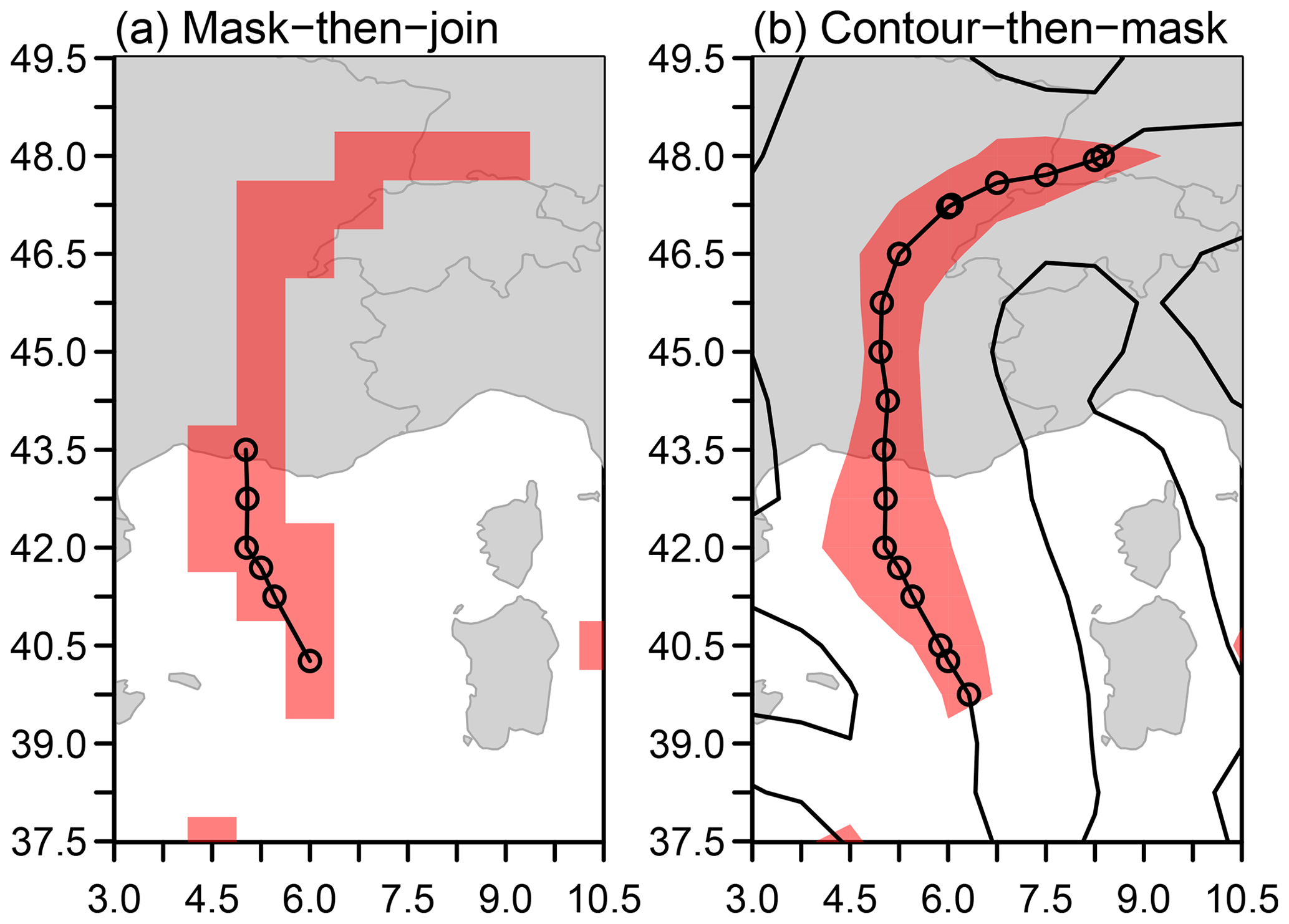
Figure 1Front identification in ERA-Interim on 1 January 2001, 00:00 UTC. (a) Using the mask-then-join approach and (b) using the contour-then-mask approach. Black contours show , and red shading indicates regions where by masking in panel (a) and interpolation in panel (b). Circles indicate front points located by each algorithm.
In contrast, H98 originally proposed a “contour-then-mask” approach, which we adopt here and illustrate in Fig. 1b. We identify zero points in the complete TFL field defined by Eq. (1) and join them into lines using a contouring algorithm, specifically the contourLines() function in R. Zero points are again located by linear interpolation, but only zero points located in adjacent grid boxes are considered for joining into lines, reducing the computational expense compared to an exhaustive search and avoiding the need for repeatedly calculating the distance between a large number of points. We then interpolate the values of the fields defined by the TFP and ABZ criteria in Eqs. (2) and (3), respectively, on the points located by the contouring algorithm. Only points that meet the TFP and ABZ criteria defined by Eqs. (2) and (3) are retained, leaving a set of pre-joined line segments representing fronts.
The two approaches are compared in Fig. 1. Zero points in Eq. (1) usually occur between grid points. That means that adjacent grid boxes meeting the TFP criteria in Eq. (2) are required in order to find zero points of the TFL using Eq. (1) by the mask-then-join approach. At or below the 0.75°×0.75° resolution of ERA-Interim, the region that satisfies the TFP criterion in Eq. (2) is often narrow, frequently only one grid box wide. Therefore, the mask-then-join approach frequently fails to locate front points. This behaviour can be seen in Fig. 1a where no front points are identified between 44.25 and 45.75° N since two zonally adjacent grid boxes would be required for successful interpolation of a zero point between two masked points given the orientation of the front. This may result in some features not being identified at all or, more frequently, gaps in what should be continuous features. The line-joining algorithm used by Berry et al. (2011b) attempts to mitigate this using a search radius larger than one grid length, but this is only partially effective. In Fig. 1a, the search radius is effective in joining the southernmost located point but fails to bridge the gap from between 44.25 and 45.75° N to the region between 46.5 and 48.0° N, where multiple adjacent grid points might once again enable the location of zero points. The number of points located in that northern region is then too small to meet the minimum front length criteria on their own. The contour-then-mask approach originally proposed by H98 and demonstrated in Fig. 1b is able to successfully identify the whole front as a single object. The masked region is shown for illustration only; in practice, the masking variables are interpolated directly onto the potential front points located on the zero contour. Overall, the contour-then-mask approach results in more fronts and front points identified and fewer breaks, as can be seen in the examples in Fig. 3a and b and the climatologies in Fig. 4b and c. The expected decrease in the number of fronts due to there being fewer breaks is compensated by the number of new fronts located due to the increased sensitivity of the contour-then-mask approach to identifying potential front points. In some cases, these new fronts were missed completely by the mask-then-join approach; in others, they fail to meet the length criteria without additional points located by the contour-then-mask approach.
3.2 Choosing the thresholds and level of smoothing
Although automated methods offer the promise of objective feature identification, it is still usually necessary to set some key parameters subjectively. For the front identification method of H98, there are three parameters that require tuning: the amount of smoothing applied to the θW field; the TFP threshold, K1; and the gradient threshold, K2. Some studies have compared outputs with manual analyses by meteorologists to calibrate the parameters. While comparing to charts is a necessary check of an objective algorithm, calibrating in this way is difficult and time-consuming and calibrates the algorithm to the subjective judgement of those meteorologists. Also, all three parameters depend on the resolution of the data. Therefore, the calibration must be repeated for each new dataset or datasets brought to a common resolution for comparison. Instead, we offer some suggestions for objective calibration criteria.
We first address the smoothing problem since the amount of smoothing applied to θW affects the choice of K1 and K2. The purpose of smoothing is to remove local minima and maxima that might break up otherwise continuous features. We particularly wish to avoid local extrema in the TFL field defined by Eq. (1), which will appear as short closed contours of . Therefore, it makes sense to examine the effect of smoothing on the average length of the contours. The noise in the TFL field will in part be due to the choice to use Eq. (1), as implemented by Berry et al. (2011b), to define the location of the fronts rather than the method preferred by H98 (their Eq. 6), designed to quell the amplification of frontal curvature. Previous studies that applied the method of Berry et al. (2011b) to ERA-Interim used n=2 passes of a simple five-point average to smooth the θW field. In testing on ERA-Interim data, it was found that the average length of the contours of initially increases rapidly with the number of passes of the five-point smoother, but after 6–10 passes, the effect of further smoothing diminishes (see Fig. S1 in the Supplement). Therefore, we settled on n=8 passes of a five-point smoother.
Equation (1) was retained for its simplicity and compatibility with Berry et al. (2011b) and subsequent studies. However, the alternative method preferred by H98 may be made available as an option in future versions of the code associated with this study. Jenkner et al. (2010) classify all closed contours in the front locating field encircling an area smaller than a given threshold as being associated with (potential) local rather than synoptic fronts. Such a criterion introduces additional subjectivity but would effectively reduce the noise when identifying synoptic fronts, possibly allowing for less smoothing to be used and further distinguish fronts associated with orography and other local features. The issue of noise- and surface-driven gradients was also discussed in Hewson (2001).
It is common to define weather phenomena as events exceeding some percentile of the climatological distribution. Therefore, we propose a quantile-based approach to setting the thresholds K1 and K2. The advantage of setting thresholds in terms of climatological quantiles is that the thresholds should be comparable between datasets of differing resolutions, while the actual values can differ quite widely. For example, Berry et al. (2011b) used a threshold for K1 of at 2.5° resolution in ERA-40 compared to the threshold of at 0.75° resolution used in ERA-Interim by Dowdy and Catto (2017). In order to compute quantiles, we require climatologies of the TFP and the magnitude of the gradient obtained by evaluating Eqs. (2) and (3), respectively, over an extended time period for the region of interest. The time period considered was 1979–2018 in ERA-Interim. Since most fronts occur in the extra-tropical regions, we will focus our attention there. We seek quantiles of the TFP and the magnitude of the gradient that produce continuous fronts in good agreement with published charts for the North Atlantic and Europe, focusing on January and July 2020. Combinations of quantiles of both the TFP and the magnitude of the gradient were systematically compared (see Figs. S2–S4 in the Supplement). We set the first threshold, K1, to the 25th percentile (0.25 quantile) of the climatological distribution of the TFP (see Fig. S2). In the Northern Hemisphere extra-tropics this is around . We set the second threshold, K2, to be equal to the 50th percentile (0.50 quantile) of the climatological distribution of the magnitude of the gradient of θW (see Fig. S3). In the Northern Hemisphere extra-tropics (23.4–66.6° N), this is around . These choices are subjective, and an operational meteorologist might make other choices. However, in the absence of strong physical reasoning, these quantiles have a simple symmetry, i.e. each is approximately the 50th percentile of the allowed range (since and, globally, the 50th percentile of TFP is approximately 0 K m−2), and produce continuous fronts in good agreement with published charts (Fig. S4).
Figure 2 illustrates the monthly and latitudinal climatological variation in the chosen quantiles of the TFP and the magnitude of the gradient of θW. The distributions of both the TFP and the magnitude of the gradient are very different in the tropics compared to the extra-tropics. The value of the TFP chosen for K1 is biased toward the upper latitudes of the Northern Hemisphere extra-tropics, where fronts are frequently observed and associated with extra-tropical cyclones. The chosen value of the magnitude of the gradient lies in the middle of the seasonal variation in the extra-tropics, which is fairly constant between around 35–65° N and 30–50° S, with greater spread in the Northern Hemisphere. The chosen values are broadly representative of the quantiles across the seasons in both the Northern and Southern Hemisphere extra-tropics. Given the relative insensitivity to reasonable values of K1 and K2 shown in the Supplement, the chosen values should be representative across the seasons and both hemispheres for both criteria.
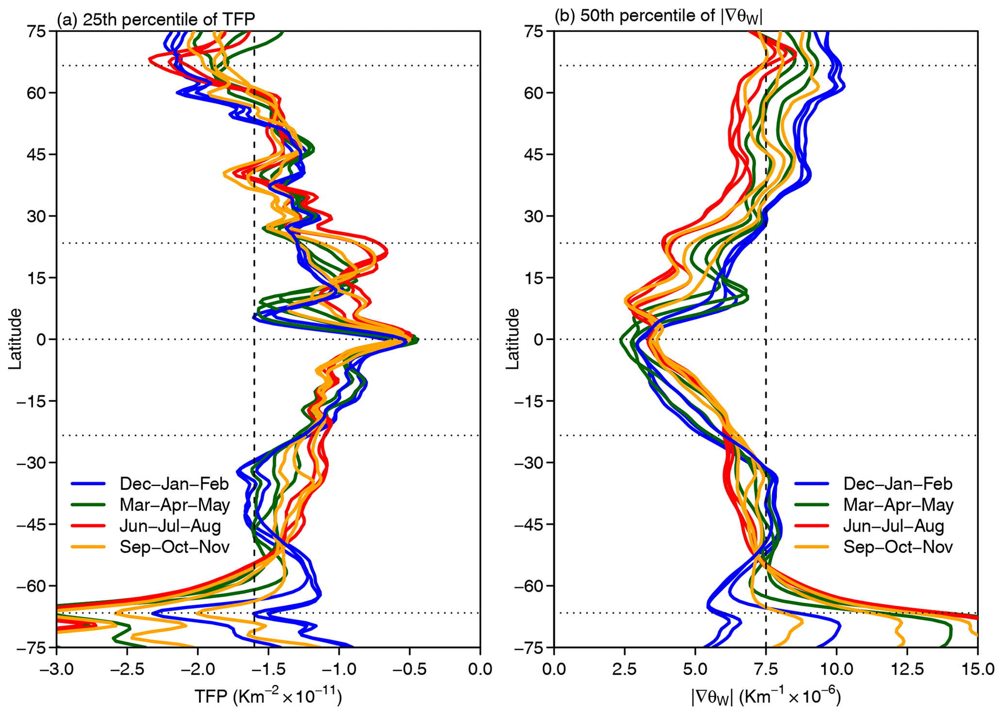
Figure 2Choosing the thresholds K1 and K2 from ERA-Interim data (1979–2018) with n=8 smoothing passes. (a) The 25th percentile of the TFP and (b) the 50th percentile of |∇θW| by latitude and month of the year. Each coloured line represents a different month: blue for December, January, and February; yellow for March, April, and May; red for June, July, and August; and orange for September, October, and November. Horizontal dotted lines represent the major circles of latitude (66.6° N, 23.4° N, 23.4° S, and 66.6° S). Vertical dashed lines indicate the thresholds chosen in the text: in panel (a) and in panel (b).
For comparison, previous studies applying the method of Berry et al. (2011b) to ERA-Interim used a threshold of after n=2 smoothing passes (e.g. Dowdy and Catto, 2017; Catto and Raveh-Rubin, 2019; Raveh-Rubin and Catto, 2019; Catto and Dowdy, 2021). The ABZ gradient threshold, K2, in Eq. (3) was not implemented by Berry et al. (2011b), which is equivalent to setting since |∇θW|≥0 by definition. Our threshold, K1, is higher primarily due to the additional smoothing, but the exclusion of the second threshold, K2, may have caused Berry et al. (2011b) to choose a lower threshold for K1 in order to remove unwanted features that could more effectively have been eliminated by implementing the second threshold, K2.
3.3 Comparing fronts from different datasets
When comparing analyses from different weather and climate datasets, the most common approach is to interpolate all the datasets to a common resolution, which is usually the lowest resolution among them. For some features, such as fronts that are more easily identified in higher-resolution data, this can be limiting. The objective calibration criteria described in Sect. 3.2 provide one route by which fronts could be identified at the native resolution of each dataset and then compared. The quantile-based criteria will identify the same fraction of grid boxes potentially containing front points for any reasonable resolution and number of smoothing passes. However, computing the required climatologies is time-consuming. An alternative is to keep the thresholds K1 and K2 constant and adjust the number of smoothing passes such that the climatological distributions of the TFP and the magnitude of the gradient are similar between datasets. Specifically, the quantiles used to set the thresholds should be similar. In testing, it was found that matching the threshold quantile of the TFP field provided a more consistent comparison than that of the gradient field. It is sufficient to compare the quantiles for only a small subset of the data, provided that the same subset is used for each dataset, avoiding the need to compute a long climatology in order to determine the thresholds. In testing, various lengths and spatial extents of training data were considered for comparing ERA-Interim and ERA5 – from 1 month to 30 years – for the Northern Hemisphere extra-tropics, Southern Hemisphere extra-tropics, or the whole globe. Finally, 1 month of data was found to be sufficient to consistently determine an appropriate number of smoothing passes. The procedure is not sensitive to either the month of the year or the spatial extent among those considered. In practice, we used January 2001 for the Northern Hemisphere extra-tropics, which is consistent with the examples in Figs. 1 and 3.
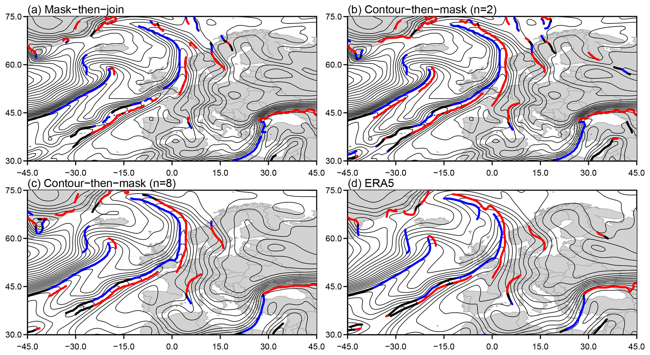
Figure 3Comparison of methods in ERA-Interim on 1 January 2001, 00:00 UTC. (a) Mask-then-join with n=2, , and ; (b) contour-then-mask with n=2, , and ; (c) contour-then-mask with n=8, , and ; and (d) contour-then-mask in ERA5 with n=96, , and . Thin black lines indicate contours of wet-bulb potential temperature θW. Thick blue lines indicate cold fronts, thick red lines indicate warm fronts, and thick black lines indicate quasi-stationary fronts. All fronts were classified using a threshold of .
3.4 Numerical updates
Berry et al. (2011b) used repeated applications of a simple central finite-difference approximation to the first derivative to evaluate all the derivatives in Eqs. (1)–(4) at each grid box. The simple approximation uses one grid box on either side of the box in question to approximate the first derivative to second-order accuracy. The zonal and meridional derivatives are evaluated separately using one box to the left and right or above and below, respectively. However, repeated applications of the approximation to the first derivative degrade the accuracy for higher derivatives. In contrast, we use an explicit central finite-difference approximation to the second derivatives required to evaluate when computing the TFL in Eq. (1), avoiding the need for repeated applications of the first derivative and maintaining second-order accuracy. The zonal and meridional terms, and , respectively, are evaluated separately. The computation of both the first and the second derivatives was also updated to maintain second-order accuracy at the edges of the domain using forward and backward differences. The increased accuracy at the edges has no additional computational cost, and the improved approximation to the second derivative is actually more efficient than repeated applications of the first derivative.
Other numerical differences include updates to the computation of relative humidity and wet-bulb potential temperature (θW). Relative humidity is required to compute wet-bulb potential temperature. If only specific rather than relative humidity data are available, relative humidity can then be computed from temperature, specific humidity, and pressure (which is constant, at 850 hPa). The implementation by Berry et al. (2011b) used the table-based approach built into the NCAR Command Language to compute relative humidity. The new implementation uses the mixed-phase parameterisation of relative humidity from the ECMWF Integrated Forecasting System (ECMWF, 2021, Sect. 7.4.2). In the new implementation, the wet-bulb potential temperature (θW) is computed using the direct method of Davies-Jones (2008, Eq. 3.8) rather than the iterative method implemented by Berry et al. (2011b). The final numerical difference between the two implementations is how short fronts are handled. In the original application, Berry et al. (2011b) reject any fronts that are less than three points long. In later applications, this was updated to a great-circle distance-based criterion where fronts whose end points are less than 250 km apart are rejected. In our implementation, we sum the great-circle distance between all adjacent points in each front and reject fronts whose total length is shorter than 250 km. The length threshold of 250 km is a subjective choice that has been retained for approximate compatibility with previous studies.
4.1 Comparison with previous implementations
Figure 3 illustrates the difference between the mask-then-join and contour-then-mask methods and the effect of the updated parameter choices (i.e. n, K1, and K2) in ERA-Interim on 1 January 2001, 00:00 UTC. The mask-then-join approach using the original parameters (Fig. 3a) clearly identifies fronts, but they are fractured with frequent gaps. The contour-then-mask (Fig. 3b) results in much smoother front features with fewer gaps and more fronts identified. Figure 3c shows the results of the updated parameters with more smoothing cycles and stronger thresholds. Figure 3d shows the fronts identified in ERA5 and is discussed further in Sect. 4.3. Compared to the original parameters, the front features are smoother, with fewer breaks, and many spurious local fronts have been removed. One feature that can be seen is a warm front running parallel to the (predominantly) cold front extending from the Azores across the south of the United Kingdom. Such features were noted by H98 and are associated with a warm conveyor belt running adjacent to the front. Hewson and Titley (2010) use a third masking criteria based on potential temperature rather than wet-bulb potential temperature that may be implemented in a future version of the code documented in this study.
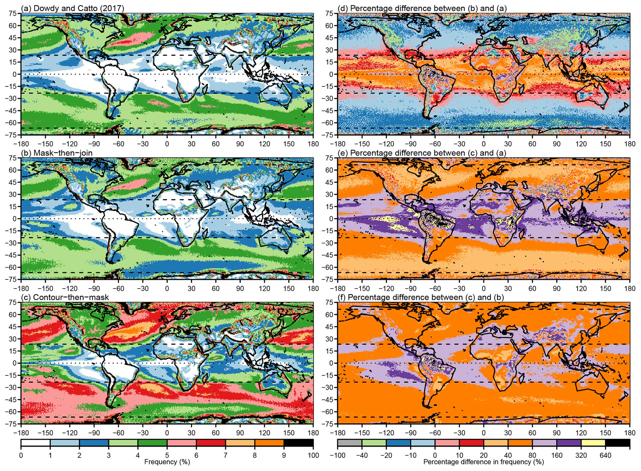
Figure 4Comparison of global climatologies of front frequency (% of 6-hourly frames from 1979–2018). (a) Dowdy and Catto (2017), (b) updated implementation using the mask-then-join approach, (c) updated implementation using the contour-then-mask approach, (d) percentage difference between mask-then-join and Dowdy and Catto (2017) ((b-a)/a), (e) percentage difference between contour-then-mask and Dowdy and Catto (2017) (), and (f) percentage difference between contour-then-mask and mask-then-join (). All climatologies were computed with n=2 smoothing cycles, , and .
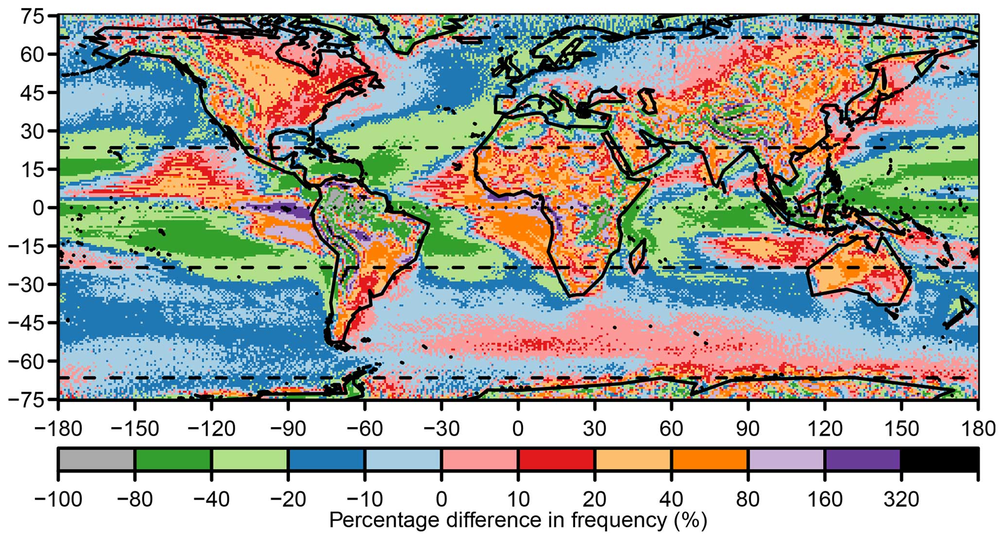
Figure 5Updated parameters. Percentage difference between ERA-Interim climatology of front frequency computed using updated parameters, n=8, , and , and the original parameters, n=2, , and .
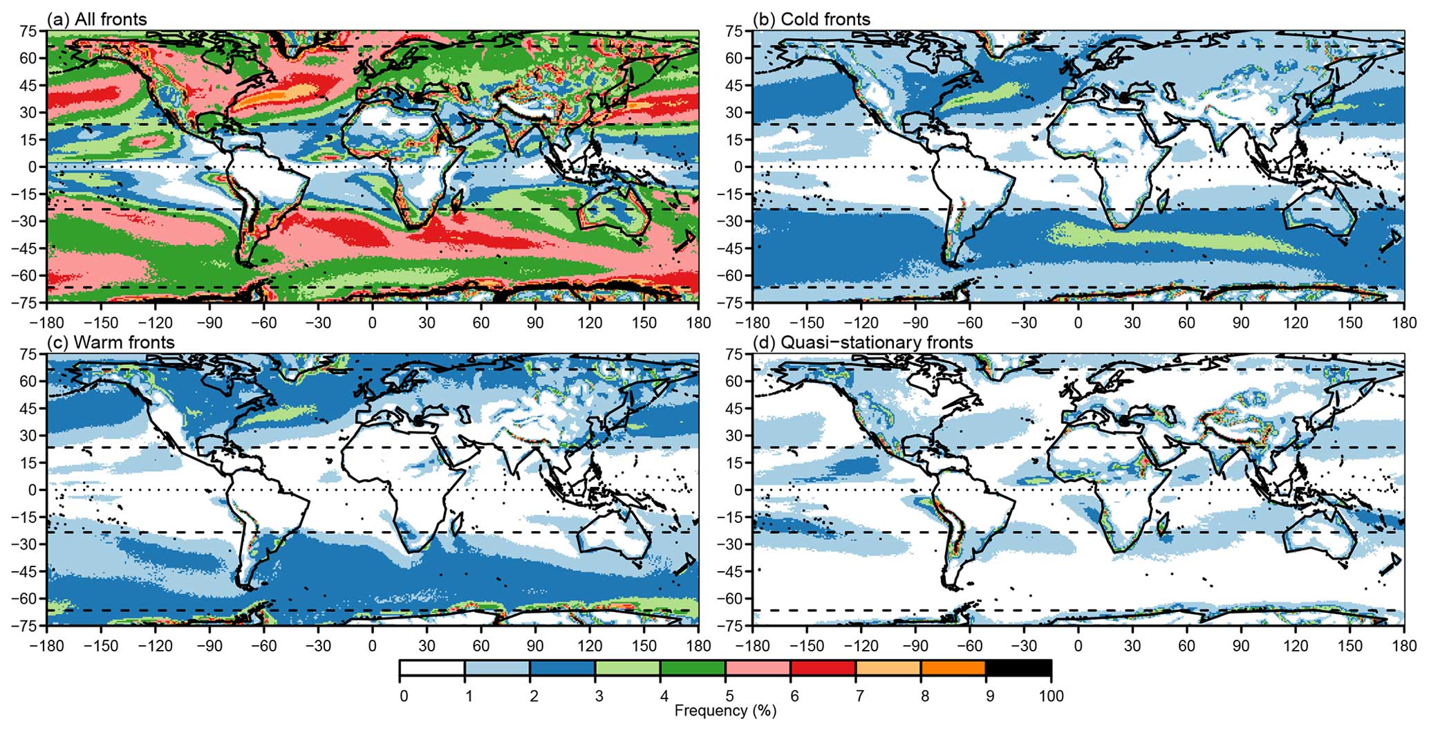
Figure 6Updated global climatologies of front frequency as a percentage of times. (a) All fronts, (b) cold fronts, (c) warm fronts, and (d) quasi-stationary fronts. All climatologies were computed with n=8 smoothing cycles, , , and .
Figure 4 compares the front frequency climatologies from three different implementations of the H98 algorithm applied to ERA-Interim with identical parameters (i.e. the same number of smoothing passes and thresholds K1 and K2): the implementation of Berry et al. (2011b) used by Dowdy and Catto (2017) (Fig. 4a), a version incorporating our numerical updates but using the original mask-then-join approach (Fig. 4b), and our final version using the contour-then-mask approach (Fig. 4c). Figure 4d shows that our numerical updates result in a slightly lower number of fronts identified in most of the Northern and Southern Hemisphere extra-tropics and a slightly higher number of fronts identified in the tropics. Figure 4e and f compare our final version with the implementation of Berry et al. (2011b) and the version incorporating only the numerical updates. The numerical updates produce relatively modest differences in the number of fronts identified (Fig. 4d). Small decreases are seen in the extra-tropics, and larger increases are seen in the tropics. The move from the mask-then-join to the contour-then-mask approach has a greater effect in the extra-tropics (Fig. 4f). In the Northern and Southern Hemisphere storm tracks, the number of fronts being identified increases by between 40 % and 80 %. The increases are a combination of increases in the length of previously identified fronts and the addition of fronts that were not previously identified, as demonstrated in Figs. 1 and 3. The greatest relative increase in the number of fronts identified is seen in the tropics. Comparing Fig. 4e and f shows that this is due to a combination of the numerical updates and the move to the contour-then-mask approach. The relative increase in the tropics is very large due to the scarcity of fronts in the tropics making even a small increase seem large. The absolute number of fronts detected in the tropics remains small compared to the extra-tropics (Fig. 4c).
While changing the implementation of the front identification leads to an increase in the number of fronts identified, as shown in Fig. 4, the next aspect of the updated method is a change to the parameters used. Figure 5 compares the climatology of front frequency of our final version with updated parameters (i.e. smoothing passes and thresholds K1 and K2; shown in Fig. 6a) applied to ERA-Interim against the implementation by Berry et al. (2011b) with the original parameters. The updated parameters result in slightly fewer fronts identified in almost all regions due to the increased smoothing, making the climatology more similar to earlier estimates but with the smoother individual fronts given by the contour-then-mask method. The greatest decreases are seen on the edges of the tropics, adjacent to regions with high front activity. This pattern is to be expected due to the rapid drop-off in the climatological quantile values of the masking parameters in the tropics in Fig. 2.
4.2 Front climatology from ERA-Interim
Figure 6 shows the climatology of front frequency of our final version with updated parameters applied to ERA-Interim, including the breakdown into cold, warm, and quasi-stationary fronts. Figure 6a allows for a direct comparison with the climatologies in Fig. 4, showing that while the updated parameters reduce the number of fronts identified compared only to the updated numerical implementation, overall, more fronts are still identified in almost all regions than in earlier versions. Figure 6b and c show that cold and warm fronts occur with similar frequencies in most extra-tropical regions, as previously shown in Berry et al. (2011b). Figure 6d shows that quasi-stationary fronts occur most often where winds are weaker, particularly in the horse latitudes close to 30° N and 30° S, the inter-tropical convergence zone (ITCZ) close to the Equator and adjacent to high orography, as expected.
Figure 7 breaks the classification of fronts down further, showing cold and warm fronts by season. Unsurprisingly, cold fronts in the Northern Hemisphere are most common at the beginning of the storm track regions of both Atlantic and Pacific oceans in northern winter (DJF; Fig. 7a). In contrast, warm fronts in northern summer (JJA; Fig. 7g) tend to outnumber cold fronts (Fig. 7c). In agreement with Berry et al. (2011b), the seasonal distribution of fronts in the Southern Hemisphere is much more stable. Cold fronts are slightly more common though less widely distributed in the Southern Hemisphere during southern summer (DJF; Fig. 7a) than in southern winter (JJA; Fig. 7c), which is consistent with Berry et al. (2011b) and the climatology of frontogenesis by Satyamurty and de Mattos (1989). The large number of warm fronts near Antarctica (JJA; Fig. 7f–h) is likely related to the strong temperature gradients between the sea surface and sea ice.
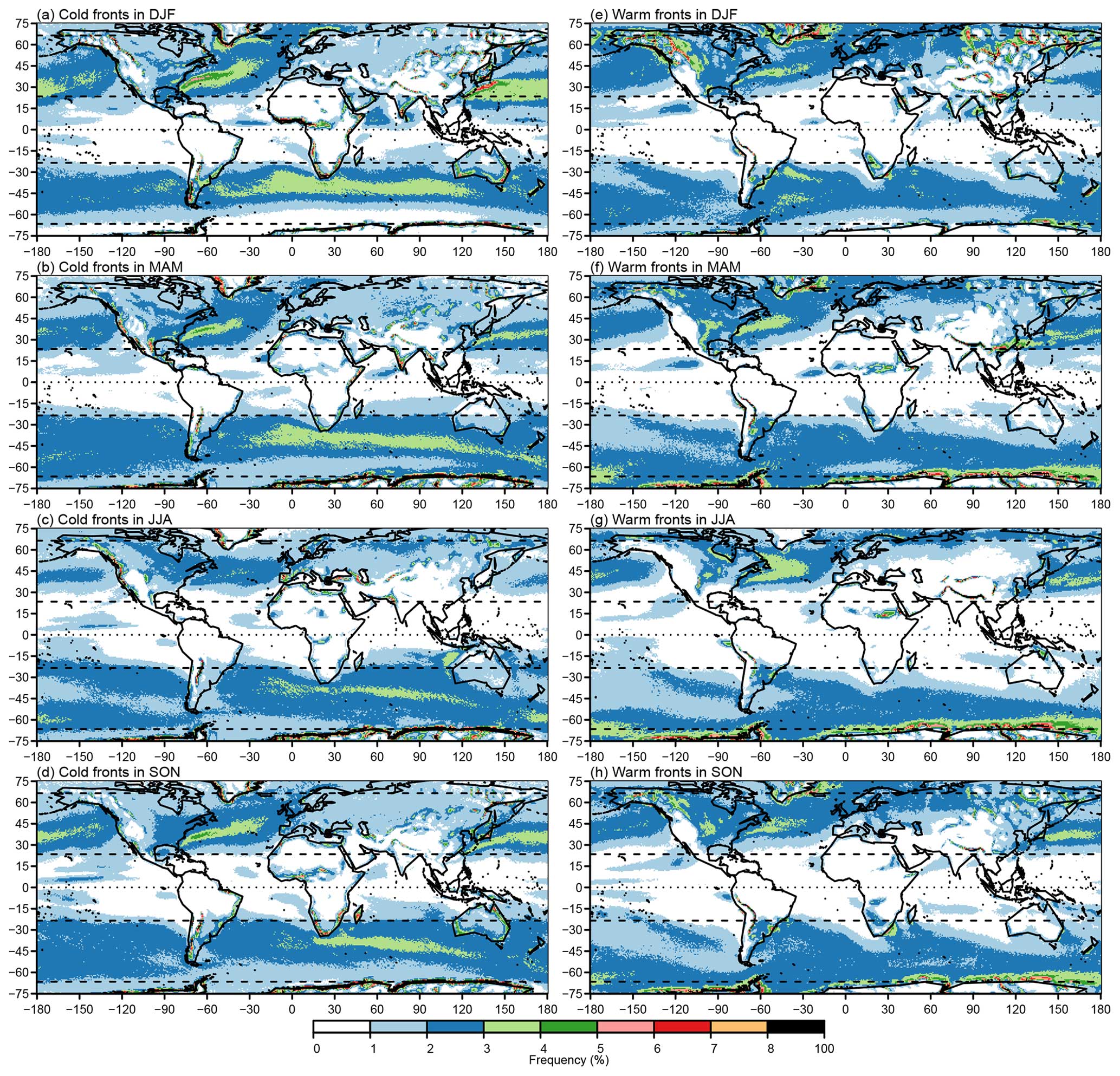
Figure 7Updated seasonal climatologies of front frequency. Cold fronts are shown in panels (a)–(d) and warm fronts in panels (e)–(h) for (a, e) DJF, (b, f) MAM, (c, g) JJA, and (d, h) SON. All climatologies were computed with n=8 smoothing cycles, , , and .
4.3 Front climatology from ERA5
The ERA5 reanalysis has a higher resolution than ERA-Interim, with a grid spacing of 0.25°×0.25° compared to 0.75°×0.75° for ERA-Interim. For ERA5, a total of n=96 smoothing cycles were required to make the climatologies of the TFP and gradient similar to ERA-Interim. Figure 3d illustrates fronts identified over Europe and the North Atlantic on 1 January 2001, 00:00 UTC. As expected, the features are very similar to those identified in ERA-Interim against which ERA5 was calibrated (Fig. 3c). Figure 8 compares the frequency of fronts identified in ERA5 with that in ERA-Interim when fronts are identified in ERA5 at 0.25°×0.25° grid spacing with n=96 smoothing cycles but identical thresholds to those used for ERA-Interim and then aggregated to 0.75°×0.75° grid spacing for comparison with ERA-Interim. Aggregation is performed by counting individual fronts identified at the higher resolution passing through the lower-resolution grid. When aggregated to the same resolution, more fronts are identified almost everywhere in ERA5 than in ERA-Interim. Since aggregation is performed by counting individual fronts, this indicates that ERA5 is able to resolve more fronts due to its higher resolution. The pattern of increase broadly follows the general distribution of fronts, with more fronts seen where they were already common, particularly in the storm tracks where front frequency increases by between 20 % and 40 %. The greatest percentage increases are seen in the ITCZ region to the east and west of South America, where very few fronts were identified in ERA-Interim (and therefore represents a very small absolute increase in frequency) and is mostly associated with quasi-stationary fronts (Fig. 9d). Decreases in frequency are primarily associated with areas of high orography, which are in turn likely associated with the improved representation of the orography in the higher-resolution dataset.
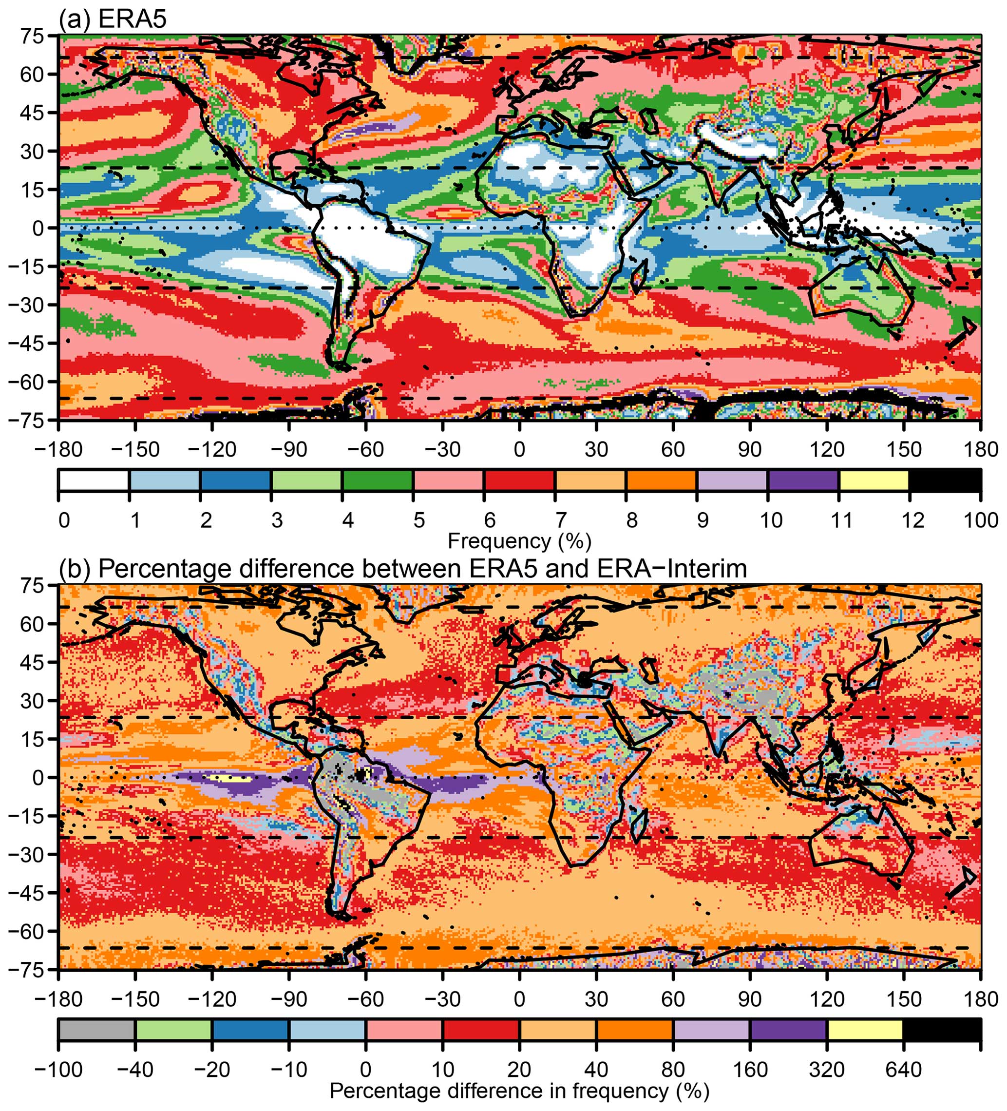
Figure 8ERA5 compared to ERA-Interim. (a) ERA5 climatology of all fronts at 0.75°×0.75° and (b) percentage difference between ERA5 and ERA-Interim. The ERA5 climatology was computed with n=96 smoothing cycles, , , and . ERA5 fronts were identified at 0.25°×0.25° and then re-gridded to 0.75°×0.75° for comparison with ERA-Interim.
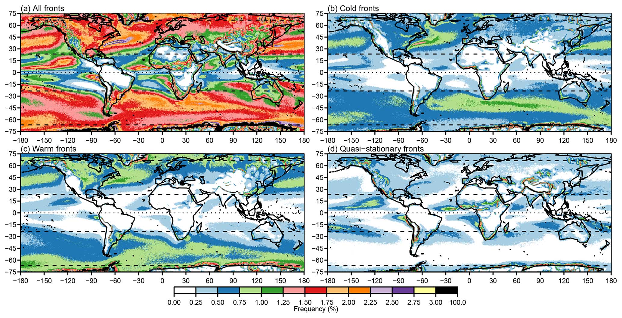
Figure 9ERA5 global climatologies. (a) All fronts, (b) cold fronts, (c) warm fronts, and (d) quasi-stationary fronts. All climatologies were computed with n=96 smoothing cycles, , , and .
Figure 9 shows the climatology of fronts by type identified in ERA5 at its native 0.25°×0.25° resolution. Due to the smaller grid boxes, the frequency is necessarily lower than for ERA-Interim in Fig. 6 and the aggregated data in Fig. 8. One ERA-Interim grid box contains nine ERA5 grid boxes. A perfectly straight front passing through one ERA-Interim grid box would typically pass through only three of the nine associated ERA5 grid boxes. Therefore, one might expect the front frequency in ERA5 at its native resolution to be approximately one-third of the frequency in ERA-Interim. Comparing Figs. 6 and 9 shows that this is approximately the case.
Figure 10 shows the seasonal breakdown of cold and warm fronts in ERA5, which is provided to be able to compare the most-up-to-date climatology from ERA5 with previous studies. In general, the maximum warm front frequency occurs at higher latitudes than the maximum cold front frequency due to the structure of extra-tropical cyclones and the associated poleward transport of warm air. During DJF especially, the high frequencies of atmospheric fronts that are influenced by the sea surface temperature (SST) fronts associated with the Gulf Stream in the North Atlantic and Kuroshio current in the North Pacific are clearly visible. The influence of the SST on the atmosphere is more marked for higher-resolution ocean and atmosphere (Parfitt et al., 2016, 2017a).
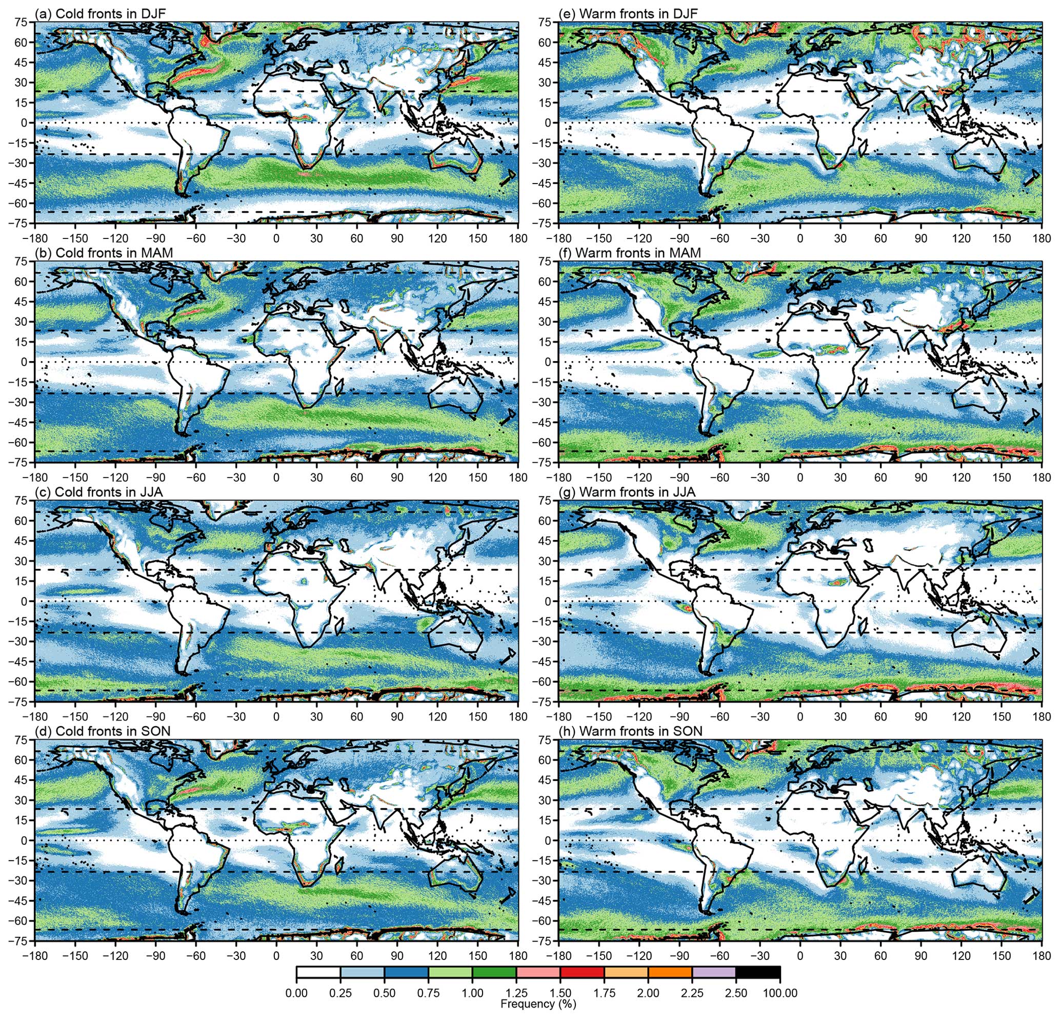
Figure 10ERA5 seasonal climatologies of front frequency. Cold fronts are shown in panels (a)–(d) and warm fronts in panels (e)–(h) for (a, e) DJF, (b, f) MAM, (c, g) JJA, (d, h) SON. All climatologies were computed with n=96 smoothing cycles, , , and .
In this paper, we have presented an updated implementation of the automatic front identification method of Berry et al. (2011b) based on H98. The updated implementation was designed specifically to scale to modern high-resolution datasets. It is open-source and does not require compilation, making it extremely portable. Despite not requiring compilation, computational performance of the new implementation in R is improved over earlier versions that were implemented in NCL with compiled components. Performance improvements come primarily from three areas: (i) the improved efficiency of the contouring algorithm compared to the line-joining algorithm, (ii) the vectorisation of many calculations to avoid unnecessary loops, and (iii) the reduced memory usage by avoiding pre-allocating unnecessarily large arrays. Indeed, 1 month of global ERA-Interim data at 6-hourly intervals and 0.75°×0.75° resolution can be processed in around 6 min using a single core of a laptop based on an Intel i7-8565U with a theoretical maximum speed of 4.6 GHz. The same amount of global ERA5 data at 0.25°×0.25° can be processed in around 1 h. Memory requirements are minimal since only one time step is processed at once. The improved scalability enables us to present high-resolution climatologies of cold, warm, and quasi-stationary fronts for all seasons from the ERA5 reanalysis.
In addition to several numerical improvements, the revised implementation uses the contour-then-mask approach originally proposed by H98 rather than the mask-then-join approach used by Berry et al. (2011b). The advantages of the contour-then-mask approach are demonstrated by example and by comparison of climatologies which show an increased number of fronts identified almost everywhere. Gaps in what should be continuous fronts are reduced in ERA-Interim, and greater improvements are expected in lower-resolution datasets for the reasons demonstrated in Fig. 1. This improvement will be useful when linking frontal features to precipitation or winds (or compound extreme events) as in Catto and Dowdy (2021) or when using more object-based connections such as Papritz et al. (2014).
Most automatic feature detection algorithms require a calibration or training step involving comparison to analyses by a meteorologist. While this step cannot be neglected, we propose a quantile-based approach to setting thresholds for front identification. Setting thresholds in terms of climatological quantiles makes the thresholds more easily comparable between datasets of differing resolution. By considering the climatological distributions of the masking variables, we have demonstrated for the first time the regional and seasonal variation in the TFP and gradient fields. Subsequent analyses may consider adopting latitudinally or seasonally varying thresholds in order to capture features that may be missed by or eliminate spurious features included by the used constant thresholds. In ERA5, this results in a greater number of fronts identified even after smoothing similarly to the results of Parfitt et al. (2017b) after interpolation to lower resolution. Smoothing has the advantage of allowing for feature identification to be conducted at the native resolution of each dataset.
In addition to the various numerical and methodological improvements presented in this study, further numerical improvements, methodological choices, and alternative choices of meteorological field are possible. In addition to improving the accuracy of the finite-difference approximations of the second derivative fields to the second order, more accurate finite-difference schemes could be used for both the first- and second-order derivatives. Following Berry et al. (2011b), we identify fronts as zero contours in the field defined by Eq. (5) of H98, which is effectively the third derivative of the wet-bulb potential temperature field at 850 hPa. Firstly, meteorological fields other than wet-bulb potential temperature could be considered; see H98 for a list of previously considered fields. Secondly, H98 derived an alternative expression for the front locator field, designed to reduce the frontal curvature. We retained the simpler definition for compatibility with Berry et al. (2011b) and subsequent studies, but the alternative definition preferred by H98 may be included as an option in a future version of the code associated with this study. Additional diagnostics, such as distinguishing between local and synoptic fronts suggested by Jenkner et al. (2010) or the additional criteria proposed by Hewson and Titley (2010) designed to eliminate spurious features associated with proximity to the warm conveyor belt, could also be implemented. Furthermore, while all distance calculations are carried out on a sphere in the updated implementation, contouring and interpolation still take place on a regular longitude–latitude grid. Greater accuracy could be achieved at high latitudes by also carrying out these operations on a sphere.
While cyclone identification algorithms routinely include the ability to track cyclonic features over subsequent time steps, similar feature-tracking algorithms are almost absent for fronts. Front tracking is inherently more complex than cyclone tracking since fronts are complex line objects, whereas cyclones can be reduced to simple point objects or point objects with an associated area. Hewson and Titley (2010) proposed a sophisticated tracking scheme for cyclonic features developing on fronts, which relies on accurate identification and classification of fronts in order to identify cyclones early in their life cycle but is limited to tracking point objects associated with cyclones rather than fronts themselves. To the authors' knowledge, only Rüdisühli et al. (2020) have documented a front-tracking algorithm. An openly available front-tracking algorithm would offer new possibilities in terms of attributing and analysing impacts of individual fronts, e.g. precipitation or wind events, or understanding biases in weather and climate models.
Code for the revised method detailed in this paper is available from https://doi.org/10.5281/zenodo.7278068 and future developments will be available at https://github.com/phil-sansom/front_id (last access: 15 August 2024). ERA5 reanalysis is available from the Copernicus Climate Change Service Climate Data Store (https://doi.org/10.24381/cds.bd0915c6, Hersbach et al., 2023)
The supplement related to this article is available online at: https://doi.org/10.5194/gmd-17-6137-2024-supplement.
PGS developed and tested the software, produced the results, and wrote the paper. JLC led the project, interpreted results, and wrote the paper.
The contact author has declared that neither of the authors has any competing interests.
Publisher's note: Copernicus Publications remains neutral with regard to jurisdictional claims made in the text, published maps, institutional affiliations, or any other geographical representation in this paper. While Copernicus Publications makes every effort to include appropriate place names, the final responsibility lies with the authors.
This research was supported by Natural Environment Research Council (NERC) (grant no. NE/V004166/1). The authors thank Duncan Ackerley for comments on the paper and the reviewers and editor for their constructive comments and support.
This research has been supported by the Natural Environment Research Council (grant no. NE/V004166/1).
This paper was edited by Jatin Kala and reviewed by two anonymous referees.
Berry, G., Jakob, C., and Reeder, M.: Recent global trends in atmospheric fronts, Geophys. Res. Lett., 38, 1–6, https://doi.org/10.1029/2011GL049481, 2011a. a, b
Berry, G., Reeder, M. J., and Jakob, C.: A global climatology of atmospheric fronts, Geophys. Res. Lett., 38, 1–5, https://doi.org/10.1029/2010GL046451, 2011b. a, b, c, d, e, f, g, h, i, j, k, l, m, n, o, p, q, r, s, t, u, v, w, x, y, z, aa, ab, ac, ad, ae, af, ag, ah
Bitsa, E., Flocas, H. A., Kouroutzoglou, J., Galanis, G., Hatzaki, M., Latsas, G., Rudeva, I., and Simmonds, I.: A Mediterranean cold front identification scheme combining wind and thermal criteria, Int. J. Climatol., 41, 6497–6510, https://doi.org/10.1002/joc.7208, 2021. a
Browning, K. A.: Conceputal Models of Precipitation Systems, Weather Forecast., 1, 23–41, https://doi.org/10.1175/1520-0434(1986)001<0023:CMOPS>2.0.CO;2, 1986. a
Browning, K. A.: The sting at the end of the tail: Damaging winds associated with extratropical cyclones, Q. J. Roy. Meteor. Soc., 130, 375–399, https://doi.org/10.1256/qj.02.143, 2004. a
Catto, J. L. and Dowdy, A. J.: Understanding compound hazards from a weather system perspective, Weather and Climate Extremes, 32, 100313, https://doi.org/10.1016/j.wace.2021.100313, 2021. a, b, c
Catto, J. L. and Pfahl, S.: The importance of fronts for extreme precipitation, J. Geophys. Res.-Atmos., 118, 10791–10801, https://doi.org/10.1002/jgrd.50852, 2013. a, b, c
Catto, J. L. and Raveh-Rubin, S.: Climatology and dynamics of the link between dry intrusions and cold fronts during winter. Part I: global climatology, Clim. Dynam., 53, 1873–1892, https://doi.org/10.1007/s00382-019-04745-w, 2019. a
Catto, J. L., Jakob, C., Berry, G., and Nicholls, N.: Relating global precipitation to atmospheric fronts, Geophys. Res. Lett., 39, 1–6, https://doi.org/10.1029/2012GL051736, 2012. a, b
Catto, J. L., Nicholls, N., Jakob, C., and Shelton, K. L.: Atmospheric fronts in current and future climates, Geophys. Res. Lett., 41, 7642–7650, https://doi.org/10.1002/2014GL061943, 2014. a, b
Catto, J. L., Ackerley, D., Booth, J. F., Champion, A. J., Colle, B. A., Pfahl, S., Pinto, J. G., Quinting, J. F., and Seiler, C.: The Future of Midlatitude Cyclones, Current Climate Change Reports, 5, 407–420, https://doi.org/10.1007/s40641-019-00149-4, 2019. a
Davies-Jones, R.: An efficient and accurate method for computing the wet-bulb temperature along pseudoadiabats, Mon. Weather Rev., 136, 2764–2785, https://doi.org/10.1175/2007MWR2224.1, 2008. a, b
Dee, D. P., Uppala, S. M., Simmons, A. J., Berrisford, P., Poli, P., Kobayashi, S., Andrae, U., Balmaseda, M. A., Balsamo, G., Bauer, P., Bechtold, P., Beljaars, A. C. M., van de Berg, L., Bidlot, J., Bormann, N., Delsol, C., Dragani, R., Fuentes, M., Geer, A. J., Haimberger, L., Healy, S. B., Hersbach, H., Hólm, E. V., Isaksen, L., Kållberg, P., Köhler, M., Matricardi, M., McNally, A. P., Monge-Sanz, B. M., Morcrette, J. J., Park, B. K., Peubey, C., de Rosnay, P., Tavolato, C., Thépaut, J. N., and Vitart, F.: The ERA-Interim reanalysis: Configuration and performance of the data assimilation system, Q. J. Roy. Meteor. Soc., 137, 553–597, https://doi.org/10.1002/qj.828, 2011. a, b
Dowdy, A. J. and Catto, J. L.: Extreme weather caused by concurrent cyclone, front and thunderstorm occurrences, Sci. Rep.-UK, 7, 1–8, https://doi.org/10.1038/srep40359, 2017. a, b, c, d, e, f, g, h
ECMWF: Part IV: Physical processes, in: IFS Documentation CY47R3, ECMWF, https://doi.org/10.21957/eyrpir4vj, 2021. a
FORTRAN 77: ANSI x3.9-1978. American National Standard – Programming Language FORTRAN, American National Standards Institute, New York, New York, https://nvlpubs.nist.gov/nistpubs/Legacy/FIPS/fipspub69-1.pdf (last access: 15 August 2024), 1978. a
Hersbach, H., Bell, B., Berrisford, P., Hirahara, S., Horányi, A., Muñoz-Sabater, J., Nicolas, J., Peubey, C., Radu, R., Schepers, D., Simmons, A., Soci, C., Abdalla, S., Abellan, X., Balsamo, G., Bechtold, P., Biavati, G., Bidlot, J., Bonavita, M., De Chiara, G., Dahlgren, P., Dee, D., Diamantakis, M., Dragani, R., Flemming, J., Forbes, R., Fuentes, M., Geer, A., Haimberger, L., Healy, S., Hogan, R. J., Hólm, E., Janisková, M., Keeley, S., Laloyaux, P., Lopez, P., Lupu, C., Radnoti, G., de Rosnay, P., Rozum, I., Vamborg, F., Villaume, S., and Thépaut, J. N.: The ERA5 global reanalysis, Q. J. Roy. Meteor. Soc., 146, 1999–2049, https://doi.org/10.1002/qj.3803, 2020. a
Hersbach, H., Bell, B., Berrisford, P., Biavati, G., Horányi, A., Muñoz Sabater, J., Nicolas, J., Peubey, C., Radu, R., Rozum, I., Schepers, D., Simmons, A., Soci, C., Dee, D., and Thépaut, J.-N.: ERA5 hourly data on pressure levels from 1940 to present, Copernicus Climate Change Service (C3S) Climate Data Store (CDS) [data set], https://doi.org/10.24381/cds.bd0915c6, 2023. a
Hewson, T. D.: Objective fronts, Meteorol. Appl., 5, 37–65, https://doi.org/10.1017/S1350482798000553, 1998. a
Hewson, T. D.: Objective identification of fronts, frontal waves and potential waves, in: Cost Action 78 Final Report – Improvement of Nowcasting Techniques, edited by: Lagouvardos, K., Liljas, E., Conway, B., and Sunde, J., European Commission EUR 19544, Cambridge University Press, Luxembourg, 285–290, 2001. a
Hewson, T. D. and Titley, H. A.: Objective identification, typing and tracking of the complete life-cycles of cyclonic features at high spatial resolution, Meteorol. Appl., 17, 355–381, https://doi.org/10.1002/met.204, 2010. a, b, c
Hope, P., Keay, K., Pook, M., Catto, J. L., Simmonds, I., Mills, G., Mcintosh, P., Risbey, J., and Berry, G.: A comparison of automated methods of front recognition for climate studies: A case study in southwest Western Australia, Mon. Weather Rev., 142, 343–363, https://doi.org/10.1175/MWR-D-12-00252.1, 2014. a
Jenkner, J., Sprenger, M., Schwenk, I., Schwierz, C., Dierer, S., and Leuenberger, D.: Detection and climatology of fronts in a high-resolution model reanalysis over the Alps, Meteorol. Appl., 17, 1–18, https://doi.org/10.1002/met.142, 2010. a, b, c
Leung, L. R., Boos, W. R., Catto, J. L., A. DeMott, C., Martin, G. M., Neelin, J. D., O'Brien, T. A., Xie, S., Feng, Z., Klingaman, N. P., Kuo, Y., Lee, R. W., Martinez-Villalobos, C., Vishnu, S., Priestley, M. D. K., Tao, C., and Zhou, Y.: Exploratory Precipitation Metrics: Spatiotemporal Characteristics, Process-Oriented, and Phenomena-Based, J. Climate, 35, 3659–3686, https://doi.org/10.1175/JCLI-D-21-0590.1, 2022. a
NCL: The NCAR Command Language, UCAR/NCAR/CISL/TDD, Boulder, Colorado, https://doi.org/10.5065/D6WD3XH5, 2011. a
Papritz, L., Pfahl, S., Rudeva, I., Simmonds, I., Sodemann, H., and Wernli, H.: The Role of Extratropical Cyclones and Fronts for Southern Ocean Freshwater Fluxes, J. Climate, 27, 6205–6224, https://doi.org/10.1175/JCLI-D-13-00409.1, 2014. a
Parfitt, R., Czaja, A., Minobe, S., and Kuwano-Yoshida, A.: The atmospheric frontal response to SST perturbations in the Gulf Stream region, Geophys. Res. Lett., 43, 2299–2306, https://doi.org/10.1002/2016GL067723, 2016. a
Parfitt, R., Czaja, A., and Kwon, Y.-O.: The impact of SST resolution change in the ERA-Interim reanalysis on wintertime Gulf Stream frontal air-sea interaction, Geophys. Res. Lett., 44, 3246–3254, https://doi.org/10.1002/2017GL073028, 2017a. a
Parfitt, R., Czaja, A., and Seo, H.: A simple diagnostic for the detection of atmospheric fronts, Geophys. Res. Lett., 44, 4351–4358, https://doi.org/10.1002/2017GL073662, 2017b. a, b, c, d
R Core Team: R: A Language and Environment for Statistical Computing, R Foundation for Statistical Computing, Vienna, Austria, https://www.r-project.org (last access: November 2022), 2021. a
Raveh-Rubin, S. and Catto, J. L.: Climatology and dynamics of the link between dry intrusions and cold fronts during winter, Part II: Front-centred perspective, Clim. Dynam., 53, 1893–1909, https://doi.org/10.1007/s00382-019-04793-2, 2019. a, b
Renard, R. J. and Clarke, L. C.: Experiments in Numerical Objective Frontal Analysis 1, Mon. Weather Rev., 93, 547–556, https://doi.org/10.1175/1520-0493(1965)093<0547:einofa>2.3.co;2, 1965. a
Rüdisühli, S., Sprenger, M., Leutwyler, D., Schär, C., and Wernli, H.: Attribution of precipitation to cyclones and fronts over Europe in a kilometer-scale regional climate simulation, Weather Clim. Dynam., 1, 675–699, https://doi.org/10.5194/wcd-1-675-2020, 2020. a
Satyamurty, P. and de Mattos, L. F.: Climatological Lower Tropospheric Frontogenesis in the Midlatitudes Due to Horizontal Deformation and Divergence, Mon. Weather Rev., 117, 1355–1364, https://doi.org/10.1175/1520-0493(1989)117<1355:CLTFIT>2.0.CO;2, 1989. a
Schemm, S., Rudeva, I., and Simmonds, I.: Extratropical fronts in the lower troposphere-global perspectives obtained from two automated methods, Q. J. Roy. Meteor. Soc., 141, 1686–1698, https://doi.org/10.1002/qj.2471, 2015. a
Schemm, S., Sprenger, M., Martius, O., Wernli, H., and Zimmer, M.: Increase in the number of extremely strong fronts over Europe? A study based on ERA-Interim reanalysis (1979–2014), Geophys. Res. Lett., 44, 553–561, https://doi.org/10.1002/2016GL071451, 2017. a
Simmonds, I., Keay, K., and Bye, J. A. T.: Identification and climatology of Southern Hemisphere mobile fronts in a modern reanalysis, J. Climate, 25, 1945–1962, https://doi.org/10.1175/JCLI-D-11-00100.1, 2012. a
Sinclair, V. A. and Keyser, D.: Force balances and dynamical regimes of numerically simulated cold fronts within the boundary layer, Q. J. Roy. Meteor. Soc., 141, 2148–2164, https://doi.org/10.1002/qj.2512, 2015. a
Soster, F. and Parfitt, R.: On Objective Identification of Atmospheric Fronts and Frontal Precipitation in Reanalysis Datasets, J. Climate, 35, 4513–4534, https://doi.org/10.1175/JCLI-D-21-0596.1, 2022. a
Thomas, C. and Schultz, D.: What are the Best Thermodynamic Quantity and Function to Define a Front in Gridded Model Output?, B. Am. Meteorol. Soc., 100, 873–895, https://doi.org/10.1175/BAMS-D-18-0137.1, 2019. a
Uppala, S. M., Kallberg, P. W., Simmons, A. J., Andrae, U., Bechtold, V. D. C., Fiorino, M., Gibson, J. K., Haseler, J., Hernandez, A., Kelly, G. A., Li, X., Onogi, K., Saarinen, S., Sokka, N., Allan, R. P., Andersson, E., Arpe, K., Balmaseda, M. A., Beljaars, A. C. M., van de Berg, L., Bidlot, J., Bormann, N., Caires, S., Chevallier, F., Dethof, A., Dragosavac, M., Fisher, M., Fuentes, M., Hagemann, S., Holm, E., Hoskins, B. J., Isaksen, L., Janssen, P. A. E. M., Jenne, R., McNally, A. P., Mahfouf, J. F., Morcrette, J. J., Rayner, N. A., Saunders, R. W., Simon, P., Sterl, A., Trenberth, K. E., Untch, A., Vasiljevic, D., Viterbo, P., and Woollen, J.: The ERA-40 re-analysis, Q. J. Roy. Meteor. Soc., 131, 2961–3012, https://doi.org/10.1256/qj.04.176, 2005. a