kNNDM CV: k-fold nearest-neighbour distance matching cross-validation for map accuracy estimation

Random and spatial cross-validation (CV) methods are commonly used to evaluate machine-learning-based spatial prediction models, and the performance values obtained are often interpreted as map accuracy estimates. However, the appropriateness of such approaches is currently the subject of controversy. For the common case where no probability sample for validation purposes is available, in Milà et al. (2022) we proposed the nearest-neighbour distance matching (NNDM) leave-one-out (LOO) CV method. This method produces a distribution of geographical nearest-neighbour distances (NNDs) between test and training locations during CV that matches the distribution of NNDs between prediction and training locations. Hence, it creates predictive conditions during CV that are comparable to what is required when predicting a defined area. Although NNDM LOO CV produced largely reliable map accuracy estimates in our analysis, as a LOO-based method, it cannot be applied to the large datasets found in many studies.

Here, we propose a novel k-fold CV strategy for map accuracy estimation inspired by the concepts of NNDM LOO CV: the k-fold NNDM (kNNDM) CV. The kNNDM algorithm tries to find a k-fold configuration such that the empirical cumulative distribution function (ECDF) of NNDs between test and training locations during CV is matched to the ECDF of NNDs between prediction and training locations.

We tested kNNDM CV in a simulation study with different sampling distributions and compared it to other CV methods including NNDM LOO CV. We found that kNNDM CV performed similarly to NNDM LOO CV and produced reasonably reliable map accuracy estimates across sampling patterns. However, compared to NNDM LOO CV, kNNDM resulted in significantly reduced computation times. In an experiment using 4000 strongly clustered training points, kNNDM CV reduced the time spent on fold assignment and model training from 4.8 d to 1.2 min. Furthermore, we found a positive association between the quality of the match of the two ECDFs in kNNDM and the reliability of the map accuracy estimates.

kNNDM provided the advantages of our original NNDM LOO CV strategy while bypassing its sample size limitations.

1 Introduction

Spatial predictive modelling using machine learning methods is commonly used in ecology and environmental sciences to predict the values of variables sampled at a limited set of locations at new, unobserved locations (see, for example, van den Hoogen et al., 2019; Sabatini et al., 2022; Moreno-Martínez et al., 2018, and Hengl et al., 2017, for global studies). A key step in the spatial prediction workflow is map accuracy assessment, i.e. the process whereby the quality of a prediction of a spatially indexed variable in a finite and defined geographical area (e.g. a set of pixels forming a continuous surface) is estimated (Stehman et al., 2021; Wadoux et al., 2021). Although map accuracy assessment should ideally be done via design-based inference based on probability sampling (Wadoux et al., 2021), this is frequently not possible due to limited access to certain areas or expensive sampling methods (Martin et al., 2012). Instead, cross-validation (CV) methods are commonly used to estimate map accuracy. Previous studies, however, have shown significant differences in map accuracy estimates depending on the type of CV being used, which has led to discussions on the appropriateness of these strategies (Wadoux et al., 2021; Meyer and Pebesma, 2022; Milà et al., 2022; Roberts et al., 2017; Ploton et al., 2020). Since CV is also typically used during model development (i.e. during hyperparameter tuning – Schratz et al., 2019 – and feature selection – Meyer et al., 2019), reliable estimates of map accuracy are crucial to developing suitable prediction models.

Traditional CV methods that ignore the spatial structure of the data such as leave-one-out (LOO) or random k-fold CV (Hastie et al., 2009) have been found to provide reliable estimates of map accuracy when samples are randomly distributed within the entire prediction area but not when they are clustered (Milà et al., 2022; Wadoux et al., 2021) or only cover parts of the prediction area (Meyer and Pebesma, 2021). As an alternative, spatial CV methods such as block CV (Wenger and Olden, 2012; Valavi et al., 2019; Roberts et al., 2017) or buffered-LOO CV (Telford and Birks, 2009; Le Rest et al., 2014; Brenning, 2022) are often used. Spatial CV methods are designed for geographical model transferability assessment, i.e. to test the ability of the model to make predictions for new geographic entities far away from the sampling areas by designing a CV where independence between training and test data is sought (Roberts et al., 2017). Such strategies, however, have been found to underestimate map accuracy when reference data are regularly or randomly distributed within the entire prediction area. In some cases, this has even been reported for clustered samples (Wadoux et al., 2021; Milà et al., 2022). Recent proposals of methods for map accuracy estimation include sampling-intensity-weighted CV, as well as model-based geostatistical approaches (de Bruin et al., 2022). However, the results of de Bruin et al. (2022) showed that these methods are not universal solutions and, depending on the sampling design, showed considerable over- or underestimation of the true map accuracy.

In our past work, we argued that the design of a CV method to provide a reliable estimate for map accuracy should be prediction-oriented; i.e. predictive conditions created during CV should resemble the conditions found when the trained model is applied to the prediction area (Milà et al., 2022; Meyer and Pebesma, 2022; Ludwig et al., 2023). Following this idea, in Milà et al. (2022) we considered predictive conditions in terms of geographical distances, and proposed the nearest-neighbour distance matching (NNDM) LOO CV method, a prediction-oriented CV method based on spatial point pattern concepts. Briefly, NNDM aims to match the empirical cumulative distribution function (ECDF) of nearest-neighbour distances (NNDs) between test and training locations in the CV to the ECDF of NNDs between prediction and training locations found during prediction.

In Milà et al. (2022) we showed that when standard LOO CV is used for reference data randomly distributed within the prediction area, the distribution of NNDs between test and training locations during CV is similar to the distribution of NNDs between prediction and training locations (see Meyer and Pebesma, 2022, for similar results for random k-fold CV). In the case of clustered sampling designs, NNDs during LOO CV were generally much shorter than prediction NNDs, which led to significant error underestimation (see also Ludwig et al., 2023). For regular samples, NNDs during LOO CV were found to be slightly longer than during prediction, leading to slight error overestimation. With the newly developed NNDM LOO CV, we could produce comparable NND distributions in most sampling designs and provide more reliable estimates of map accuracy that can be used during model development or to indicate the accuracy of the predictions.

Even though NNDM LOO CV showed promising results across different sampling designs, prediction areas, and landscape autocorrelation ranges, the fact that it is a LOO-based CV method hinders its broader application given its high computational cost in medium and large datasets. To overcome this limitation, our aim is to extend the idea of NNDM LOO CV to a k-fold NNDM CV, hereafter kNNDM, that can be applied to larger datasets commonly found in ecology and the environmental sciences.

This article is organised as follows: after presenting our algorithm in Sect. 2, in Sect. 3 we reproduce the simulation study included in Milà et al. (2022) to assess the performance and run-time of kNNDM compared to other CV methods including NNDM LOO. In this simulation, we also explore the influence of the number of folds k and the relationship between the quality of the match and the quality of the estimation of the map accuracy. As supplementary material (Appendix A), we provide a second simulation study, which we also briefly describe in Sect. 3. Finally, Sect. 4 discusses the strengths and limitations of our method and suggests future lines of work.

2 Algorithm description

The objective of kNNDM is to find a k-fold configuration such that the distribution of NNDs between test and training locations during CV matches as closely as possible the distribution of NNDs between prediction and training locations. In other words, kNNDM aims to create predictive conditions in terms of geographical distances that resemble those found when using the model to predict a certain area. To do so, we use a clustering approach to create a set of candidate fold configurations with different degrees of spatial clustering, of which we choose the one that offers the best match between the two distributions. Before explaining the algorithm in detail, we define the different NND distribution functions used in kNNDM, as well as the statistic used to evaluate the different fold candidates.

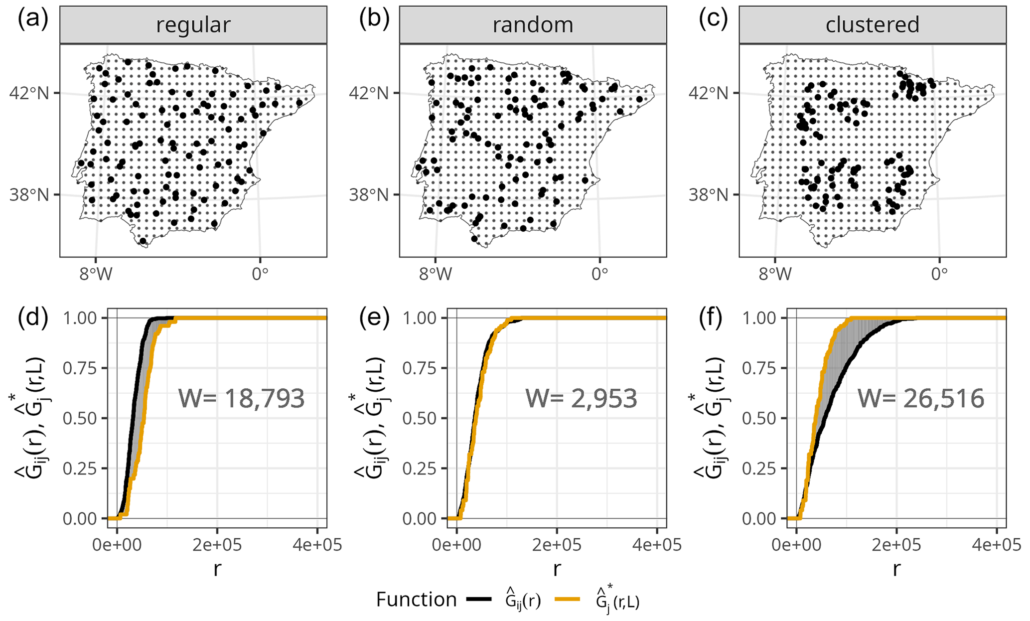
Figure 1 (a–c) Prediction points (regular grid) and training points with different spatial distributions (bold), simulated for visualisation purposes only. (d–f) NND ECDF between training and test locations during 10-fold random CV (${\widehat{G}}_j^{*}(r,\mathbf{L})$, orange) and NND ECDF between prediction and training locations (${\widehat{G}}_{ij}\left(r\right)$, black) corresponding to each of the sampling distributions in the top row. The shaded grey area corresponds to the W statistic, whose value is printed in the plots.

As in the original NNDM LOO algorithm, in kNNDM we define nearest-neighbour distance distribution functions by means of their NND ECDF, where j is the index for training points, i is the index for prediction points, and r is a distance (Euclidean for projected coordinates and spherical for geographical coordinates).

• ${\widehat{G}}_j\left(r\right)$ is the NND ECDF between test and training locations during LOO CV and expresses the proportion of training points that have another training point at a distance less than or equal to r:

  $${\widehat{G}}_j\left(r\right)={\displaystyle \frac{\mathrm{1}}{n_j}}\sum _j\mathrm{1}\mathit{\{}{d}_j\le r\mathit{\}},\text{where}{d}_j=\underset{k\ne j}{min}\parallel x_j^{\left(j\right)}-x_k^{\left(j\right)}\parallel .$$

• ${\widehat{G}}_{ij}\left(r\right)$ is the NND ECDF between prediction and training locations and expresses the proportion of prediction points that have a sampling point at a distance less than or equal to r:

  $${\widehat{G}}_{ij}\left(r\right)={\displaystyle \frac{\mathrm{1}}{n_i}}\sum _i\mathrm{1}\mathit{\{}{d}_{ij}\le r\mathit{\}},\text{where}{d}_{ij}=min\parallel x_i^{\left(i\right)}-x^{\left(j\right)}\parallel .$$

• ${\widehat{G}}_j^{*}(r,\mathbf{L})$ is the NND ECDF between test and training locations during a CV defined in L and expresses the proportion of test points that have a training point at a distance less than or equal to r during a given CV strategy. Note that $\mathbf{L}=\mathit{\{}{\mathbf{l}}_{\mathrm{1}},{\mathbf{l}}_{\mathrm{2}},\mathrm{\dots },{\mathbf{l}}_{n_j}\mathit{\}}$ is a list of sets l_j containing the indices of the samples to fit the model to when holding out observation j during CV. Note that since in kNNDM we leave out data points in folds rather than one by one, l_j will be exactly the same for all samples belonging to the same fold:

  $${\widehat{G}}_j^{*}(r,\mathbf{L})={\displaystyle \frac{\mathrm{1}}{n_j}}\sum _j\mathrm{1}\mathit{\{}{d}_j^{*}\le r\mathit{\}},\text{where}{d}_j^{*}=\underset{k\in {\mathbf{l}}_j}{min}\parallel x_j^{\left(j\right)}-x_k^{\left(j\right)}\parallel .$$

Another important component of our approach is how to measure the quality of the match between ${\widehat{G}}_j^{*}(r,\mathbf{L})$ and ${\widehat{G}}_{ij}\left(r\right)$ given a fold configuration. We do that using the Wasserstein statistic (Dowd, 2020; Vaserstein, 1969), which compares the distribution of two samples by calculating the integral of the absolute value differences between the two ECDFs. In our case, we define W as the integral over the geographical distances r of the absolute value differences between ${\widehat{G}}_j^{*}(r,\mathbf{L})$ and ${\widehat{G}}_{ij}\left(r\right)$:

$$W=\int \left|{\widehat{G}}_j^{*}\right(r,\mathbf{L})-{\widehat{G}}_{ij}(r\left)\right|\text{d}r.$$

Small values of W indicate that the two ECDFs are similar, while W will be larger if they differ. To illustrate this point, we show the calculation of the W statistic between ${\widehat{G}}_j^{*}(r,\mathbf{L})$ and ${\widehat{G}}_{ij}\left(r\right)$ for a random 10-fold CV and different sampling patterns (Fig. 1). As shown in Meyer and Pebesma (2022), when samples are randomly distributed within the prediction area, the distribution of NNDs during the random 10-fold CV ${\widehat{G}}_j^{*}(r,\mathbf{L})$ resembles the distribution of NNDs during prediction ${\widehat{G}}_{ij}\left(r\right)$, and therefore the value of W is small. However, in the presence of clustered samples, random k-fold CV NNDs are shorter than prediction NNDs, and thus ${\widehat{G}}_j^{*}(r,\mathbf{L})>{\widehat{G}}_{ij}\left(r\right)$, resulting in a large W value. The opposite occurs when training samples follow a regular sampling pattern, also leading to a larger W statistic compared to random sampling.

Now that the definitions of the NND functions and the W statistic have been stated, we proceed with the explanation of the kNNDM algorithm (Fig. 2). The required inputs include the georeferenced training and prediction points, the desired number of folds k, and the clustering algorithm to be used. The first step is to test whether the training points are clustered with respect to the prediction points; to do that we compute ${\widehat{G}}_j\left(r\right)$ and ${\widehat{G}}_{ij}\left(r\right)$ and then test the null hypothesis H₀, i.e. G_j(r)≤G_ij(r), vs. the alternative hypothesis H₁, i.e. G_j(r)>G_ij(r), with a one-sided Kolmogorov–Smirnov (KS) two-sample test (Conover, 1999). If the null hypothesis is not rejected, the algorithm returns a random k-fold CV, since it is the appropriate option for random and regular samples (Meyer and Pebesma, 2022; Wadoux et al., 2021; de Bruin et al., 2022). If, however, the null hypothesis is rejected (p value < 0.05), we proceed to cluster the training points based on their coordinates into a series of q∈Q clusters, where Q is defined as an integer sequence of length 100 ranging between k and N (the total number of training points) equally spaced on a logarithmic scale and back-transformed, to try configurations with a small number of clusters more intensively. Currently, hierarchical and k-means clustering methods are implemented.

Figure 2 Workflow of the kNNDM algorithm.

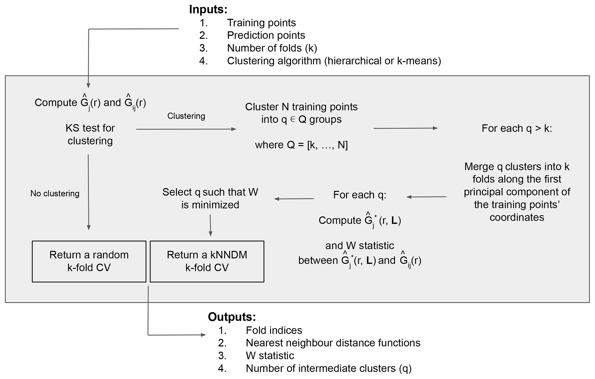
Next, for every configuration where q>k, we merge the resulting q clusters into the final k folds along the first principal component of the coordinates of the training points to prevent contiguous clusters in space to be in the same fold. Briefly, we compute the first principal component of the training points' coordinates to capture the direction with the most spatial variability, project the q cluster centroids into that first component and order them according to it, and finally merge q clusters into k folds by giving different fold levels to contiguous clusters in that dimension. Large clusters with a proportion greater than $\mathrm{1}/k$ of the training data are not merged to keep fold balance. Once this procedure is completed, we compute ${\widehat{G}}_j^{*}(r,\mathbf{L})$ and W for each fold configuration candidate and select the one with the smallest W, i.e. the one that provides the best match between ${\widehat{G}}_j^{*}(r,\mathbf{L})$ and ${\widehat{G}}_{ij}\left(r\right)$. As outputs, the algorithm returns the fold indices of the selected configuration, as well as their respective NND functions, W statistic, and intermediate number of folds q.

As an illustration of how kNNDM works in cases where samples are clustered within the prediction area, Fig. 3 shows a 2-fold kNNDM CV configuration for different numbers of clusters q, their respective NND ECDFs, and the W statistic between ${\widehat{G}}_j^{*}(r,\mathbf{L})$ and ${\widehat{G}}_{ij}\left(r\right)$ assessing the match. A low number of clusters leads to a strong partition of the geographical space and long NNDs between test and training points during CV, which are actually longer than NNDs encountered when predicting from all reference data. As the number of clusters increases, ${\widehat{G}}_j^{*}(r,\mathbf{L})$ gets closer to ${\widehat{G}}_j\left(r\right)$, i.e. the NND ECDF encountered during LOO CV. In this example, the kNNDM algorithm would select the configuration with q=21, since it minimises the W statistic, i.e. provides the best match.

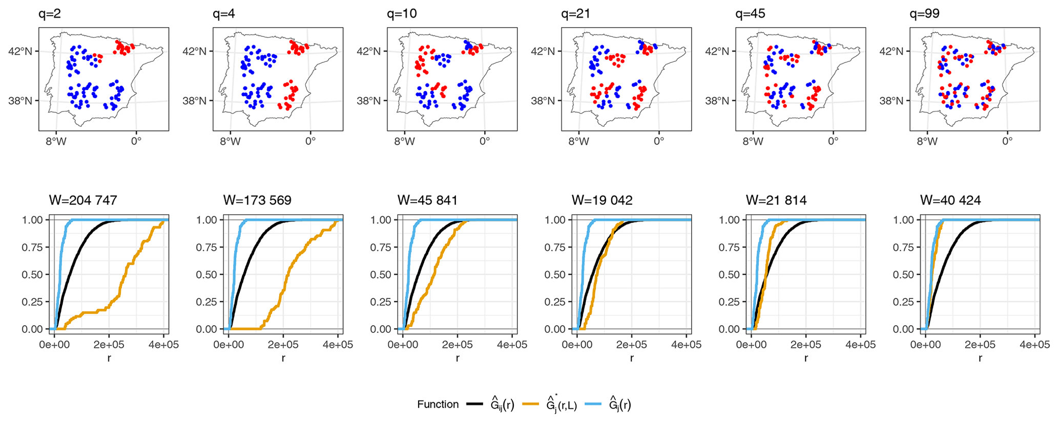
Figure 3 Top row: kNNDM with k=2 (red and blue points) for several clusters q. Prediction points consist of a regular grid (not shown) spanning the whole polygon. Points were simulated for visualisation purposes only. Bottom row: NND ECDF between training locations during LOO CV (${\widehat{G}}_j\left(r\right)$, blue), between test and training locations during kNNDM CV (${\widehat{G}}_j^{*}(r,\mathbf{L})$, orange), and between prediction and training locations (${\widehat{G}}_{ij}\left(r\right)$, black) corresponding to each CV configuration in the top row.

As practical considerations, in our implementation we have provided the possibility, as an alternative to the prediction points' input, of supplying a polygon defining the prediction area, from which prediction points are sampled internally. Moreover, we have included a balancing parameter for the maximum single fold size allowed that discards non-compliant fold candidates. Regarding computational performance, our algorithm benefits from using projected coordinates since fast nearest-neighbourhood searches in Euclidean space can be performed using the FNN package (Beygelzimer et al., 2022). Finally, when using kNNDM we recommend computing accuracy statistics such as the coefficient of determination (R²), the root mean square error (RMSE), or the mean absolute error (MAE) in the stacked out-of-sample predictions rather than performing an average of the statistics computed in each of the folds, since the resulting folds can be unbalanced and ${\widehat{G}}_j^{*}(r,\mathbf{L})$ is constructed using all CV folds simultaneously (Meyer et al., 2023).

3 Simulation studies

3.1 Algorithm performance for map accuracy estimation

To investigate the performance of kNNDM CV and how it compares to the original NNDM LOO CV, we used the same simulation as in our previous work (see Milà et al., 2022, for a complete description). Briefly, we generated a virtual response surface, i.e. a spatially indexed continuous variable between 0 and 1, using a selection of WorldClim bioclimatic variables for the Iberian Peninsula (Fig. 4a) and the virtualspecies R package (Leroy et al., 2015). Next, we simulated training locations with five different distributions and a sample size of 100 (Fig. 4b). We performed 100 iterations of the sampling simulation, and, in each of them, we extracted the predictor (bioclimatic variables) and response data at the sampling points' locations and fitted random forest (RF) regression models, resulting in a total of 500 fitted models. RF hyperparameters were not tuned, and default values were used in all simulations to shorten computation time.

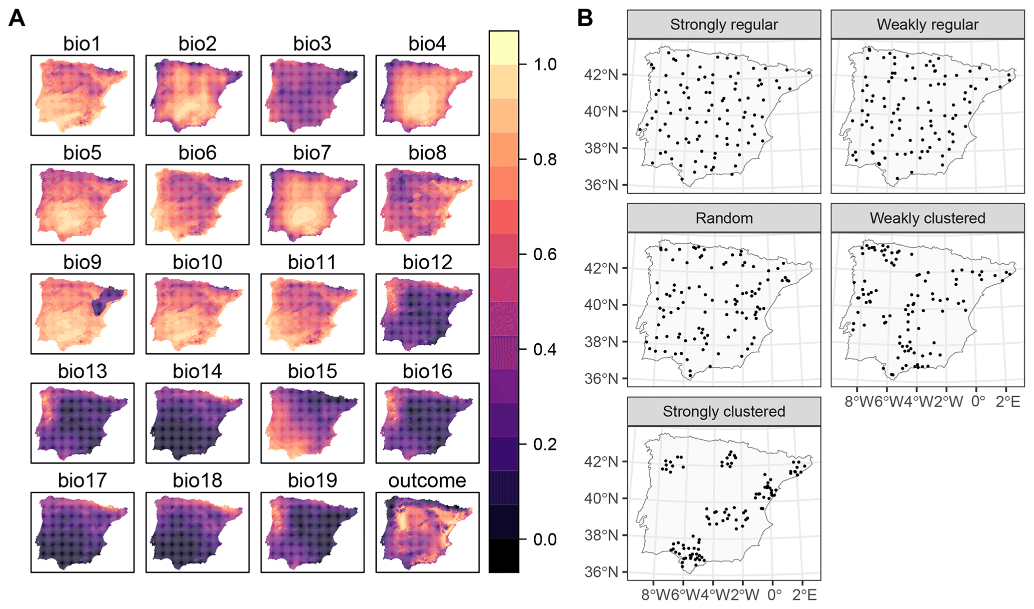
Figure 4 Data used in the simulation: (a) bioclimatic covariates and response (all linearly stretched to [0,1] for visualisation purposes) and (b) an example of one iteration of the sample simulation. Figure reproduced from Milà et al. (2022).

Each fitted RF model was used to predict the response in the entire prediction area, from which the true map accuracy was calculated (RMSE, MAE, and R²). Additionally, we used the following CV methods: (1) random 10-fold CV, (2) spatial 10-fold CV via k-means clustering (Brenning, 2012), (3) the original NNDM LOO CV, and (4) 10-fold kNNDM CV. In contrast to the original simulation in Milà et al. (2022), here we matched all distances in the prediction area during NNDM rather than up to a certain range estimated from the data. In order to interpret results, we subtracted the true map accuracy metrics from each of the CV estimates to assess their performance (Fig. 5).

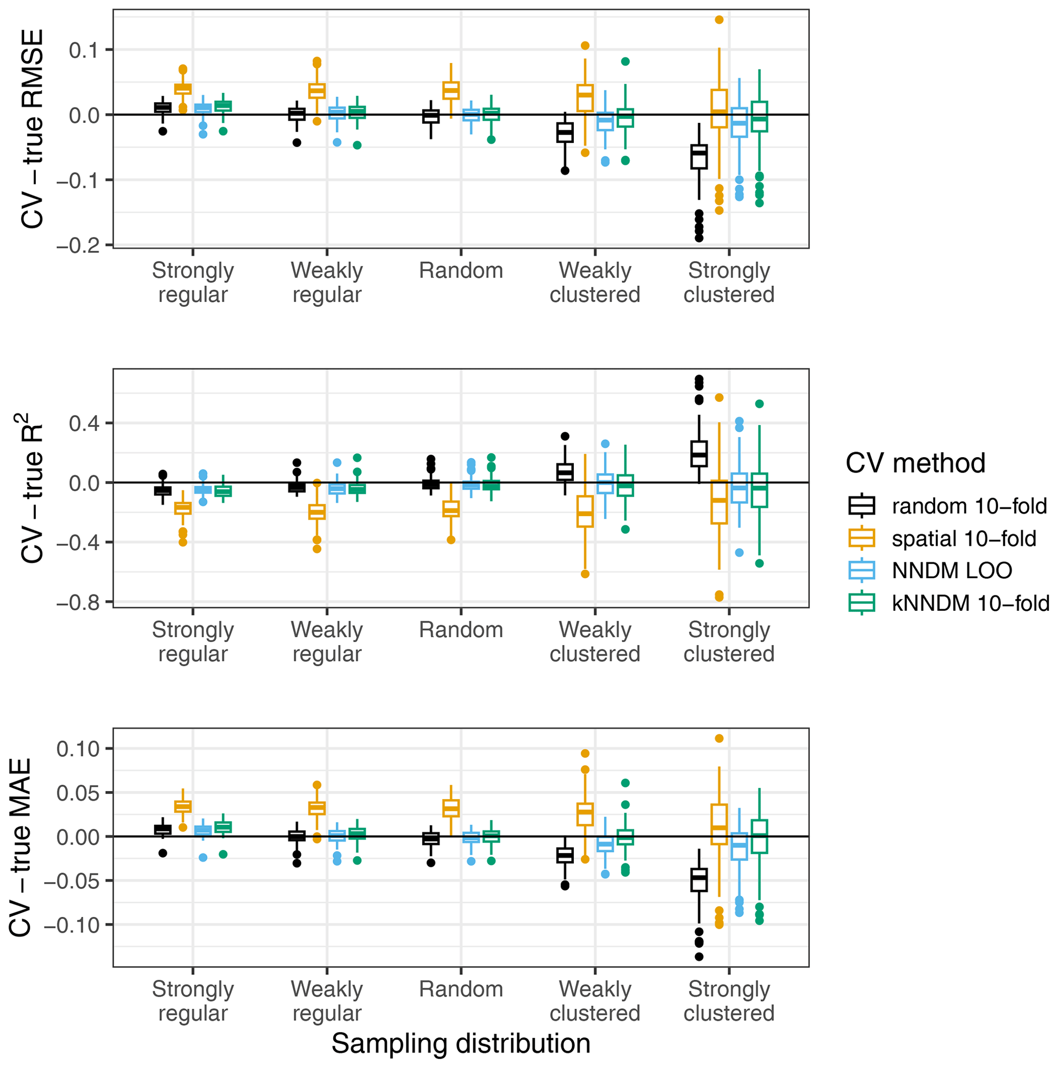
Figure 5 Differences between cross-validated and true RMSE, R², and MAE by sampling distribution and CV method for the simulated virtual response variable.

The kNNDM CV yielded reliable error estimates across all sampling patterns we considered, which were similar and in some cases even more accurate than those estimated via NNDM LOO CV (Fig. 5). Variability in the differences was larger in kNNDM than in NNDM LOO CV for strongly clustered samples. Random 10-fold CV produced reliable estimates under random sampling patterns but failed for clustered data. The spatial 10-fold CV overestimated the mapping error except for the RMSE in the strong clustering scenario and had the largest variability.

3.2 Relationship between the quality of the match and the quality of the map accuracy estimate

In order to investigate the relationship between the quality of the match in kNNDM and the quality of the map accuracy metrics, we performed a second simulation using the same response and predictors and 100 iterations of our first simulation (Sect. 3.1). However, in this second simulation, we (1) added two more extremely clustered sample configurations to extend the range of possible W values; (2) only used kNNDM CV; (3) did not check for clustering as a first step in kNNDM, i.e. applied the clustering approach to all samples regardless of their distribution; and (4) kept all candidate fold configurations considered within kNNDM, q_i∈Q, and their respective values of the W statistic, rather than just the one yielding the lowest W. We used all of these candidate CV splits to calculate CV map accuracy statistics, and we computed the absolute value difference with respect to the true value of the map accuracy statistic. We then plotted these absolute value differences against the corresponding W statistic and fitted a linear regression to summarise the trend (Fig. 6).

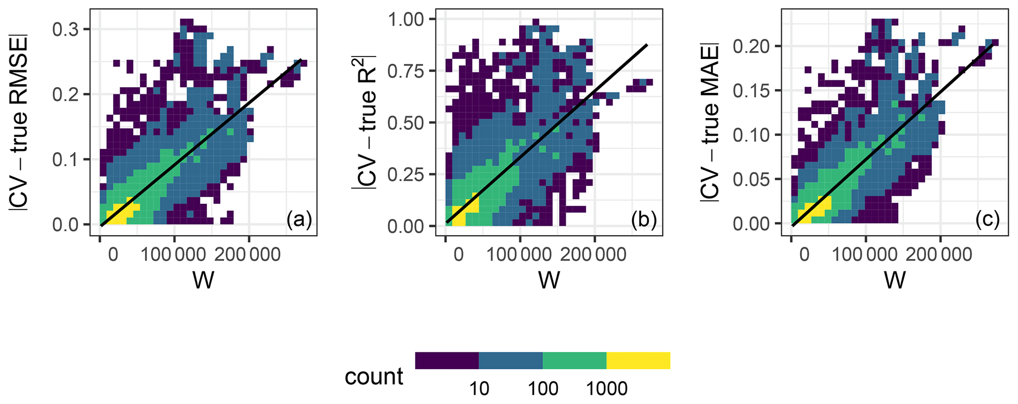
Figure 6 Relationship in 10-fold kNNDM between the absolute value difference between the CV and true map accuracy statistics (y axis) and W statistic (x axis) for the RMSE (a), R² (b), and MAE (c) statistics. Colour represents the data point density. The black line shows the linear regression fit. The R² values of the regression models are 0.66, 0.6, and 0.73 for the RMSE, R², and MAE, respectively.

The relationship between the absolute value differences between CV and true map accuracy statistics (Fig. 6) and W showed that, for all three statistics considered, a poor match between ${\widehat{G}}_j^{*}(r,\mathbf{L})$ and ${\widehat{G}}_{ij}\left(r\right)$ indicated by a greater W statistic led to poor estimates of the true map accuracy, while the true map accuracy could be better estimated for well-matching functions. This positive association was linear for all three statistics with at least 60 % explained variance.

3.3 Influence of the number of folds

The choice of k can influence the performance of kNNDM to a certain extent since it dictates the maximum clustering that can be achieved. To investigate the influence of k, we repeated the workflow described in Sect. 3.1 but only employed kNNDM CV using an even integer sequence $k\in \mathit{\{}\mathrm{2},\mathrm{4},\mathrm{6},\mathrm{\dots },\mathrm{20}\mathit{\}}$. In each of the 100 iterations, we calculated the true and estimated error metrics, as well as the quality of the match between the ECDF of NNDs between CV folds (${\widehat{G}}_j^{*}(r,\mathbf{L})$) and the ECDF of NNDs between prediction points and sample points (${\widehat{G}}_{ij}\left(r\right)$) as measured by the Wasserstein statistic (W). With the resulting statistics, we plotted the distribution of the differences between the estimated and true RMSE, MAE, and R² as well as the W statistic for each k value (Fig. 7).

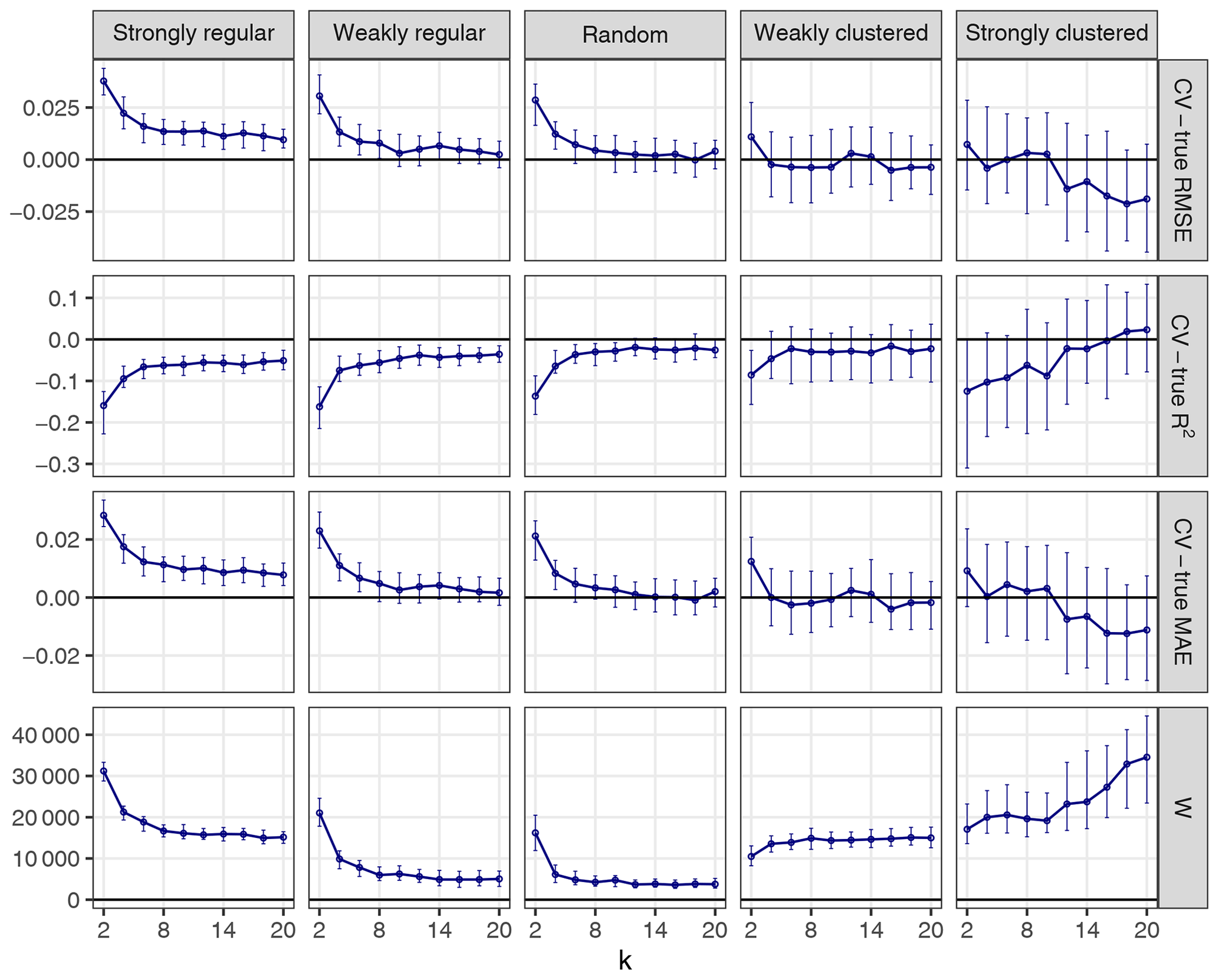
Figure 7 CV error estimates for kNNDM CV with different values of k (first three rows). The respective W statistic is shown in the fourth row. Points indicate median values, while error bars show the first and third quartile.

Our results indicated that a larger number of folds resulted in better matches for regular and random samples but worse matches for strongly clustered designs. While, for regular and random samples, this translated into increasingly accurate map accuracy estimates for a larger number of folds, for clustered data, the number of folds with the smallest W value, i.e. k=2, was overly pessimistic and k=4 or 6 actually performed better.

3.4 Run-time analysis

Since our goal was to propose a computationally feasible alternative to NNDM LOO CV for large datasets, we performed a run-time analysis to quantify the speed gains of kNNDM CV compared to NNDM LOO CV. We separately quantified the time spent on (1) finding the optimal CV split (i.e. running the NNDM LOO and kNNDM algorithms); (2) repetitively fitting the model according to the CV configuration; and (3) the total run-time, i.e. the sum of (1) and (2). We did that using the same simulation framework as in Sect. 3.1 but with 50 different sample sizes, ranging from 100 to 4000 training points. We only used the strongly clustered and the random sampling designs for computational reasons. We used a maximum of 4000 training points, since the computational time exceeded 1 week per run for NNDM LOO CV. The analysis was carried out using a high-performance computation cluster utilising up to 1.5 GB of RAM for each run using the Intel^® Xeon^® Gold 6140 CPU.

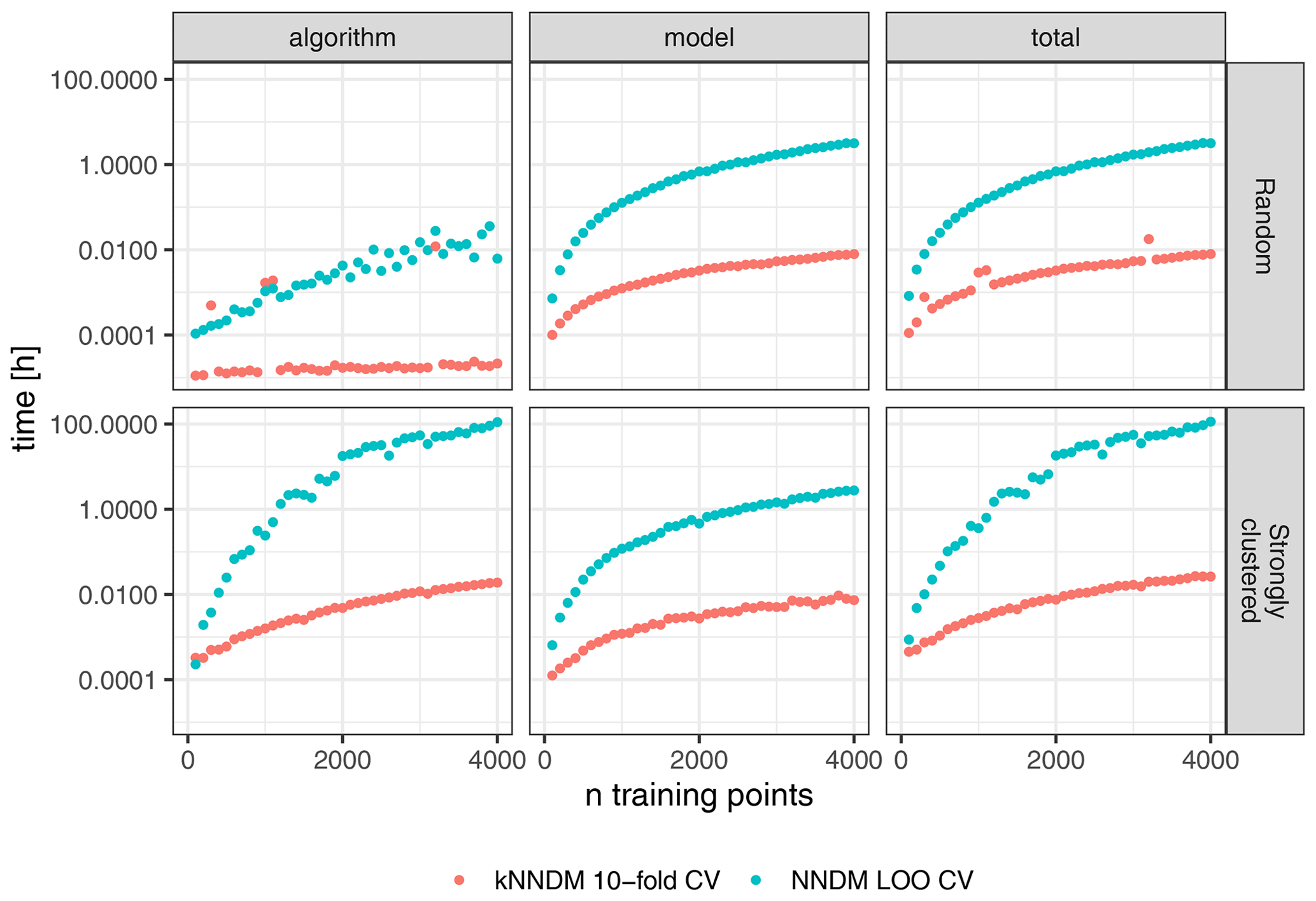
Figure 8 Differences in computational time (log-scaled) between 10-fold kNNDM CV (red) and NNDM LOO CV (blue) for two different sample designs (rows).

The run-time analysis showed large speed gains of kNNDM CV compared to NNDM LOO CV under all tested sample designs (Fig. 8). For the random sampling design, the kNNDM algorithm was especially fast due to the prior test for clustering in the training data. This test returns a simple random k-fold CV when no clustering is detected and is much faster than running the entire kNNDM algorithm (see Sect. 2). Only in four cases did the test not return a random CV, and in those four cases the computational times were longer (red outliers in Fig. 8).

NNDM LOO was slower compared to kNNDM when the training data were randomly distributed and much slower when they were clustered (Fig. 8). For a sample size of 4000, kNNDM CV reduced the time spent on fold assignment and model training from 3.2 h to 30 s for random samples and from 4.8 d to 1.2 min for clustered samples as compared to NNDM LOO CV. Furthermore, the computational time of NNDM LOO CV increased exponentially with increasing sample size. This pattern arises from both the architecture of the NNDM LOO CV algorithm (Fig. 8, left column) and from the difference between LOO CV and k-fold CV in terms of model fitting, since NNDM LOO CV requires training k=N models, while the number of models trained during k-fold CV is usually much smaller, in this case k=10 (Fig. 8, middle column).

3.5 Additional simulation study

To test the robustness of our results, we tested the performance of kNNDM CV in a second simulation using a real-world dataset described in detail in Appendix A and used in the study by de Bruin et al. (2022). Briefly, we modelled above-ground biomass in Europe using different sampling distributions ranging from regular to strongly clustered (Fig. A1).

Results for the second simulation broadly agreed with the first simulation, although we observed some differences that are worth pointing out. The 10-fold kNNDM reliably estimated the true RMSE in all designs except in the strongly clustered one, where, similarly to spatial CV, it resulted in overly optimistic estimates (Fig. A2). The relationship between the absolute value difference between CV and true RMSE was positive but only explained 28 % of the total variance (Fig. A3). While large numbers of folds resulted in a better match as expressed by W and more accurate RMSE for regular and random designs (Fig. A4), in strongly clustered designs the opposite was observed. For weak clustered results, k=4 had the lowest W statistic although RMSEs were also estimated well for larger values of k.

4 Discussion

In this work, we propose a new prediction-oriented CV strategy for map accuracy estimation named kNNDM, which takes into account the geographical prediction space of the model. The kNNDM approach extends the ideas of NNDM LOO CV to a k-fold CV strategy that can be used for medium and even large reference datasets to estimate map accuracy in the absence of probability sampling test data. In the simulation study, kNNDM performed similarly to NNDM LOO CV and produced reasonably reliable map accuracy estimates for most sampling patterns. Thus, kNNDM provided the advantages of our original NNDM LOO strategy while bypassing its sample size limitations. Small differences between NNDM LOO and kNNDM CV can be attributed to the different ways to match the distributions as well as the different hold-out sample size.

Similarly to other studies (e.g. Wadoux et al., 2021; de Bruin et al., 2022), we observed that random k-fold CV returned reliable estimates of map accuracy with randomly distributed samples within the prediction area, while it was overly optimistic when samples were clustered. Also in agreement with other studies, we found that spatial CV methods that do not take into account the geographical prediction space tended to be overly pessimistic even with clustered samples within the prediction area (Wadoux et al., 2021; de Bruin et al., 2022; Milà et al., 2022), for example as a result of block sizes that do not match the prediction task. A unique finding of our study that deserves special attention is the positive association we found between the W statistic measuring the quality of the match of the NND ECDFs during CV and prediction and the quality of the estimation of the map accuracy statistics. This association was strong in our first simulation, which had a national scale, supporting our suggestion to design CV strategies that try to match the predictive conditions of the models in terms of geographical NNDs. That said, this relationship was weaker in the second simulation, where the study area had a continental scale. This suggests that other factors such as distances in the feature space may also play a role in the performance of CV map accuracy estimates.

Our experiments showed that the number of folds can have an impact on the performance of kNNDM. For randomly and regularly distributed samples, k needs to be sufficiently large (k≥10) to provide accurate estimates of map accuracy. The same finding applies to random k-fold CV, to which kNNDM generalises for random and regular samples. We attribute this to the fact that, when the number of clusters is small, neighbouring samples can be put in the same fold with a probability that increases with smaller k values. On the other hand, for severely clustered samples, a smaller number of folds may be beneficial as k determines the maximum clustering that can be achieved when the geographical space is partitioned into k contiguous blocks. The suitability of a smaller number of folds was indicated by a higher quality of the match shown by the Wasserstein statistic. Comparing the suitability of different fold configurations via the Wasserstein statistic can be used for guidance when choosing the number of folds. Nonetheless, in clustered settings where W indicates that the best match is achieved by setting a very low k such as k=2 (see Fig. 7), we recommend taking a larger fold size such as 4 or 5 since the amount of bias expected with two folds due to large parts of the training data being left out is expected to be large (Kohavi, 1995) and is likely the reason that we observe better results for k=4 or 6 in our experiments.

Even though kNNDM overcomes the sample size limitations of NNDM LOO CV, there are still limitations of the approach. First, the flexibility of the matching in kNNDM is lower than in NNDM LOO CV, since every observation must be assigned to a fold. Moreover, it is also possible that the range of NNDs observed during prediction is different than the range of NND between training points, which might make the match impossible for some distances. This is especially the case when the prediction area is different from the training area (i.e. complete model transfer). For these reasons, the match between CV and prediction NND ECDF in kNNDM may not always be possible and an inspection of the NND ECDF like in Fig. 1 should always be conducted. Similarly, if training data are very clustered within the prediction area as in the strongly clustered design of the second simulation, kNNDM may still fail to offer a CV configuration that matches the predictive conditions. In that case, we recommend users allow for a greater maximum fold size or ask for a lower fold number k to account for potentially larger clusters. Furthermore, in cases where this is still not sufficient, we recommend restricting the prediction area to the area of applicability (AOA) of the model (Meyer and Pebesma, 2021) to limit the effects of feature extrapolation. Secondly, both kNNDM and NNDM LOO CV algorithms are currently solely based on the geographical space; therefore, if the feature distribution between the training and prediction locations is very different, a feature-based CV strategy might be more appropriate (Roberts et al., 2017). For example, Wang et al. (2023) recently developed a CV method that considers both the geographic and the feature space, although it does not consider the prediction domain and predictive conditions of the model. Thirdly, NNDM-based CV methods do not address the small error overestimation for regular samples that we found in our simulations, so map accuracy estimates will tend to be slightly conservative in such cases. Fourthly, NNDM-based methods are purely based on geographical distances and ignore the location of the training points or the direction of the distances, which can be problematic if non-stationarity or anisotropy of the errors is present (Brenning, 2022). Fifthly, the CV error estimate obtained by kNNDM is only reasonable if the prediction area does not change when the model is deployed. If the prediction area changes significantly, re-evaluation might be required. Also, when the prediction area is unknown prior to model training, kNNDM cannot be used.

Possible future points for investigation regarding kNNDM include (1) conducting a simulation study comparing newly proposed CV-based map accuracy estimation methods (de Bruin et al., 2022) as well as feature-based CV methods (Roberts et al., 2017) in a larger variety of scenarios, also including classification problems; (2) implementing a genetic algorithm that minimises the W statistic directly as a function of CV folds; (3)  exploring the extension of kNNDM to feature space (an experimental version is already implemented in the CAST package; evaluation via simulation studies still pending); and (4) investigating how kNNDM CV can affect feature selection (Meyer et al., 2019), hyperparameter tuning (Schratz et al., 2019), and model applicability (Meyer and Pebesma, 2021). A further possible extension to the kNNDM algorithm is the exclusion of training points during CV, which might help to achieve a better match in strongly clustered designs without the need to increase fold sizes. Furthermore, it might be beneficial to develop and integrate a one-sided Wasserstein test instead of using the Kolmogorov–Smirnov two-sample test to test whether the training points are clustered as the first step of the algorithm, since the Wasserstein test has a greater power than the Kolmogorov–Smirnov one (Dowd, 2020) and would also be more consistent with the rest of the algorithm, which uses the Wasserstein statistic as well.

Finally, we would like to emphasise again that NNDM and kNNDM CV do not replace established strategies to estimate map accuracy via design-based inference (as outlined in Wadoux et al., 2021), which should always be preferred. Nonetheless, prediction-oriented CV methods such as NNDM LOO or kNNDM CV that consider the prediction objectives of the model can be used to implement a measure of map accuracy during model development or, in the absence of a probability sample, to estimate the map accuracy of a given model.

Appendix A: Additional simulation study

This appendix describes a second simulation study used to assess the robustness of our findings. We used the example presented in de Bruin et al. (2022), where a set of 22 predictor variables (see Appendix A of de Bruin et al., 2022, for a list of the predictor variables and data sources) was used to predict above-ground biomass (AGB; Santoro and Cartus, 2021) in Europe using different sampling designs (Fig. A1). This dataset was used to test the same hypotheses as in our main simulation with the following specific objectives: (1) to test the ability of kNNDM to estimate true map accuracy, (2) to assess the relationship between the quality of the match and the quality of the map accuracy estimate, and (3) to explore the impact of the number of folds on the performance of kNNDM. All methods and visualisations follow our main simulation as much as possible to allow for comparison.

To test the ability of kNNDM to estimate the map accuracy (first objective), random forest (RF) models with fixed default hyperparameters were trained on 5000 sample points generated by five sampling designs ranging from regular to clustered (Fig. A1) as in de Bruin et al. (2022). Then, their predictive performance (measured as the root mean square error, RMSE) was estimated using different types of cross-validation (CV) and was compared to the true RMSE for the entire surface. Namely, we assessed the performance of random 10-fold CV, spatial 10-fold CV based on k-means clustering of the geographical coordinates (Brenning, 2012), and 10-fold kNNDM CV. We did not include NNDM LOO CV, since it was computationally not feasible (see Fig. 7 in the main paper for a run-time analysis). While in the original study by de Bruin et al. (2022) the CV split was repeated 100 times per sample distribution and CV error estimates were averaged, we only used one repetition to shorten computational times. For a more detailed description of the simulation, we refer the reader to de Bruin et al. (2022). We subtracted the estimated and the true RMSE and plotted the distribution of these differences by CV method (Fig. A2).

To assess the relationship between the quality of the match and the quality of the map accuracy estimate (second objective), we repeated the workflow described in the first objective but (1) only used kNNDM CV; (2) did not check for clustering as a first step in kNNDM, i.e. applied the clustering approach to all samples regardless of their distribution; and (3) kept all candidate fold configurations considered within kNNDM, q_i∈Q , and their respective values of the W statistic, rather than just the one yielding the lowest W. We used all of these CV configurations to estimate map accuracy, and we computed the absolute value difference between the estimates and the true value. We then plotted these differences against the corresponding W statistic and fitted a linear regression to estimate the relationship between the two (Fig. A3).

To explore the impact of the number of folds on the performance of kNNDM (third objective), we repeated the workflow described in the first objective but employed kNNDM CV using an even integer sequence $k\in \mathit{\{}\mathrm{2},\mathrm{4},\mathrm{6},\mathrm{\dots },\mathrm{20}\mathit{\}}$. In each of the 100 iterations, we calculated the true and estimated RMSE, as well as the quality of the match as measured by the Wasserstein statistic (W). With the resulting statistics, we plotted the distribution of the differences between the estimated and true RMSE as well as the W statistics (Fig. A4).

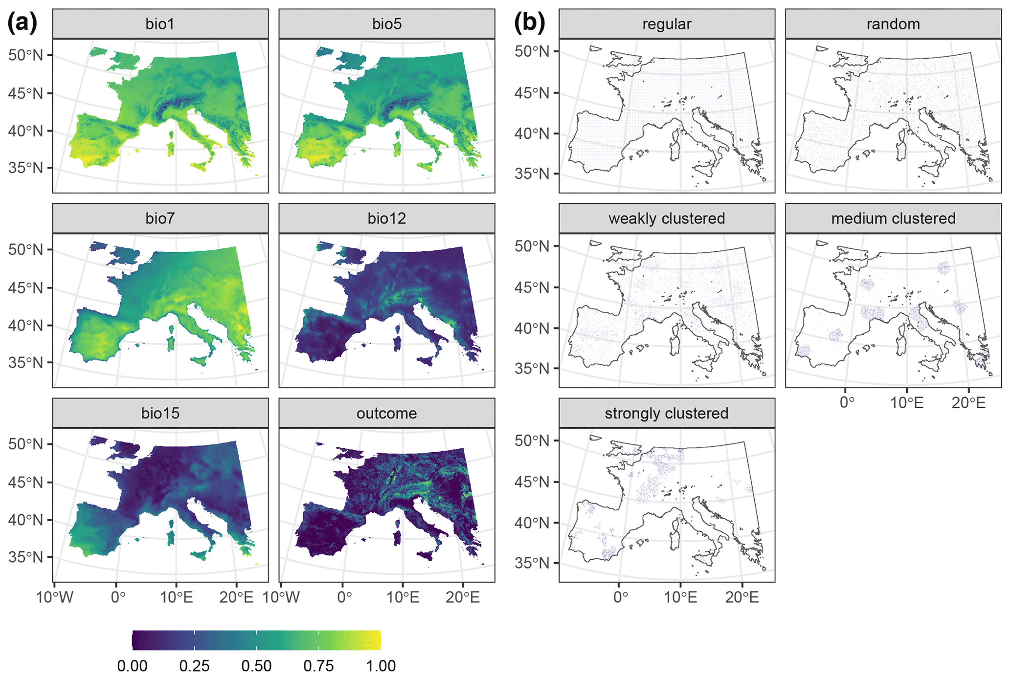
Figure A1 Data used in the AGB simulation. Panel (a) shows a subset of the 22 predictors, as well as the response raster. Rasters were linearly stretched to [0,1] for visualisation purposes. Panel (b) shows one iteration of the different sampling designs. Data from de Bruin et al. (2022).

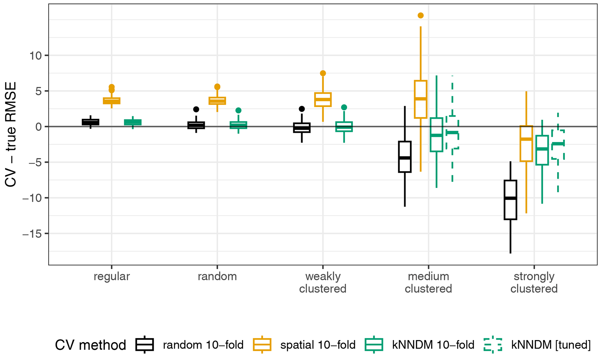
Figure A2 Differences between cross-validated and true RMSE; “kNNDM [tuned]” refers to the kNNDM split that yielded the lowest W statistic among different numbers of folds $k\in \mathit{\{}\mathrm{2},\mathrm{4},\mathrm{6},\mathrm{\dots },\mathrm{20}\mathit{\}}$.

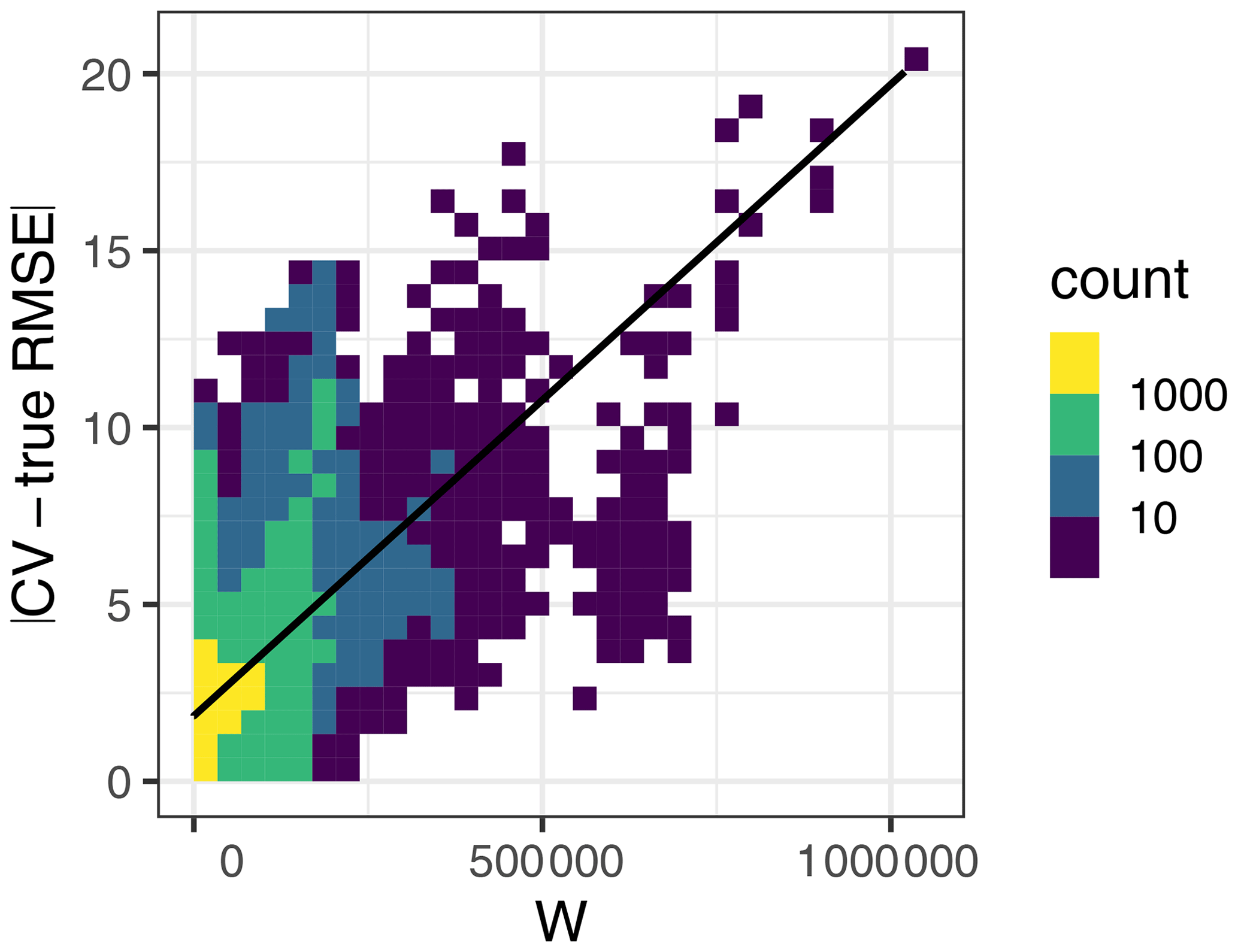
Figure A3 Relationship between the absolute value difference between the CV and true RMSE (y axis) with the W statistic (x axis). Here, W explained 28 % of the variation in the absolute value RMSE differences.

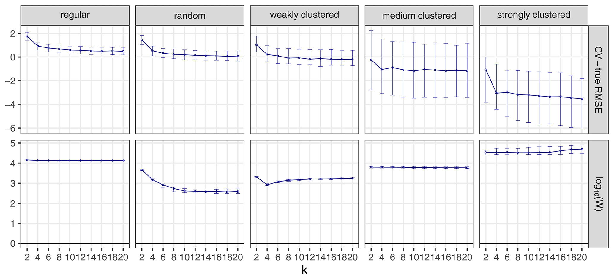
Figure A4 The influence of different numbers of k on the difference between the cross-validated and true RMSE (upper row) and on the W statistic (lower row). Points indicate median values, while error bars show the first and third quartile. Note that the values of the W statistic are log-scaled.