the Creative Commons Attribution 4.0 License.
the Creative Commons Attribution 4.0 License.
 | 24 Jul 2024
Reduced floating-point precision in regional climate simulations: an ensemble-based statistical verification
Christian Zeman
David Leutwyler
Stefan Rüdisühli
Christoph Schär
The use of single precision in floating-point representation has become increasingly common in operational weather prediction. Meanwhile, climate simulations are still typically run in double precision. The reasons for this are likely manifold and range from concerns about compliance and conservation laws to the unknown effect of single precision on slow processes or simply the less frequent opportunity and higher computational costs of validation.
Using an ensemble-based statistical methodology, Zeman and Schär (2022) could detect differences between double- and single-precision simulations from the regional weather and climate model COSMO. However, these differences are minimal and often only detectable during the first few hours or days of the simulation. To evaluate whether these differences are relevant for regional climate simulations, we have conducted 10-year-long ensemble simulations over the European domain of the Coordinated Regional Climate Downscaling Experiment (EURO-CORDEX) in single and double precision with 100 ensemble members.
By applying the statistical testing at a grid-cell level for 47 output variables every 12 or 24 h, we only detected a marginally increased rejection rate for the single-precision climate simulations compared to the double-precision reference based on the differences in distribution for all tested variables. This increase in the rejection rate is much smaller than that arising from minor variations of the horizontal diffusion coefficient in the model. Therefore, we deem it negligible as it is masked by model uncertainty.
To our knowledge, this study represents the most comprehensive analysis so far on the effects of reduced precision in a climate simulation for a realistic setting, namely with a fully fledged regional climate model in a configuration that has already been used for climate change impact and adaptation studies. The ensemble-based verification of model output at a grid-cell level and high temporal resolution is very sensitive and suitable for verifying climate models. Furthermore, the verification methodology is model-agnostic, meaning it can be applied to any model. Our findings encourage exploiting the reduction of computational costs (∼30 % for COSMO) obtained from reduced precision for regional climate simulations.
- Article
(3365 KB) - Full-text XML
- BibTeX
- EndNote


Numerical weather and climate models have evolved from simple and computationally inexpensive radiative–convective models (Manabe and Wetherald, 1967) into highly complex codes solving the governing equations on billions of grid points. While this advancement improves the representation of Earth's climate, it also increases computational costs, storage requirements, and energy consumption (Schär et al., 2020). Reducing these costs without compromising model accuracy is crucial for further enhancements of resolution, domain size, ensemble size length of integration, number of variables, and quality of parameterization schemes.
Reducing the precision in floating-point representation is a straightforward method to alleviate computational costs in numerical simulations. Typically, a floating-point number in weather and climate models requires 64 bits (double precision; DP). Reducing the precision to 32 bits (single precision; SP) will reduce the dynamical range (±10308 for DP, ±1038 for SP) and the accuracy (machine precision; for DP, for SP) of numbers. Take the representation of temperature for instance. In DP, temperature can be represented with a very high level of detail: for example, 296.45678912345676 K. In SP, the number of digits could be reduced to 296.4568 K.
For most calculations within a climate model, the range and accuracy of SP are more than enough, especially when considering the often substantial uncertainties associated with discretization, physical parameterizations for subgrid-scale processes, initial and boundary condition errors, and emission scenarios. On the plus side, the use of SP instead of DP can significantly reduce the computational costs of a simulation due to higher arithmetic intensity (number of floating-point operations per number of bytes transferred between cache and shared memory) and a reduction of internode communication, as SP allows for fitting twice as many grid points into the memory of a single node compared to DP.
Reduced precision is used operationally by MeteoSwiss for the national weather forecast for Switzerland. They implemented SP for most model components, observing no discernible impact on forecast skill (Rüdisühli et al., 2014). While the switch to SP did not require any major code changes, some modifications like the reformulation of specific formulas and the addition of precision-dependent epsilons were necessary for the comparison of floating-point numbers (i.e., ABS(a-b) < eps) and to avoid division by zero (see Rüdisühli et al., 2014, for an overview). A few model components still rely on DP, namely parts of the radiation and the soil model, making the implementation “mixed precision” rather than purely SP. The reduction in computational costs from using COSMO with reduced precision is likely highly dependent on model configuration (model domain, domain decomposition, parameterizations used, etc.) as well as computer architecture and compiler settings. Previous studies with COSMO have shown the reduction in computational costs to be around 30 % (Zeman and Schär, 2022) or 40 % (Rüdisühli et al., 2014).
The Unified Model (Brown et al., 2012) from the Met Office operationally uses SP in the iterative solver for the Helmholtz equation in the dynamical core, which leads to improved runtime with no detrimental impact on the accuracy of the solution (Maynard and Walters, 2019).
Düben and Palmer (2014) performed global simulations with the European Centre for Medium-Range Weather Forecasts (ECMWF) Integrated Forecasting System (IFS; ECMWF, 2023) at SP for several days at horizontal grid spacings ranging from 950 to 32 km. The differences in 500 hPa geopotential and 850 hPa temperature between SP and DP were consistently smaller than those between different DP ensemble members of the standard ensemble forecasting system.
Váňa et al. (2017) performed 13-month-long global simulations at ∼50 km grid spacing with four ensemble members (generated by shifting the initial times) using the IFS in DP and SP, with the SP runs having around 40 % shorter runtimes. They compared the results with observations and found only minor differences in root mean square errors (RMSEs) from annual means of several model quantities between the DP and SP versions. These differences were negligible when considering the magnitude of systematic forecast errors.
Nakano et al. (2018) evaluated SP for parts of the Nonhydrostatic Icosahedral Grid Atmospheric Model (NICAM; Satoh et al., 2014) using the Jablonowski and Williamson baroclinic wave benchmark test (Jablonowski and Williamson, 2006). By using DP for the model setup and SP everywhere else, the simulations showed the same quality as those with the conventional DP model but could be performed 1.8 times faster.
Klöwer et al. (2020) investigated the effect of 16-bit precision on a shallow-water model and found that without mitigation methods such as rescaling, reordering, or using higher precision for critical parts of the code, 16-bit arithmetic induced rounding errors that were too big. They also showed that using the Posit number format (Gustafson and Yonemoto, 2017) reduced the forecast error compared to the traditional IEEE 754 format. Ackmann et al. (2022) performed idealized tests with a shallow-water model and showed that at least some parts of the elliptic solvers of the semi-implicit time-stepping schemes could be performed at half-precision without negatively affecting the quality of the solution when compared to only using DP.
Extensive testing with reduced precision for IFS was conducted by Lang et al. (2021). They performed medium-range ensembles consisting of 50 members with a forecast range of 15 d for several periods at a grid spacing of 18 km and 91 or 137 vertical levels. The simulations were validated using the continuous ranked probability score (CRPS; Matheson and Winkler, 1976) against model analysis and observations for 121 variables, and significance has been tested with the Student's t test combined with variance inflation accounting for temporal autocorrelation following the approach by Geer (2015). Compared to the DP ensemble with 91 levels, the SP ensemble with 91 levels had a reduced runtime by approximately 40 % (the same as Rüdisühli et al., 2014, and Váňa et al., 2017) without compromising forecast skill. Moreover, the SP ensemble with 137 levels significantly improved forecast skill while still having about 10 % shorter runtime than the DP ensemble with 91 levels. Based on these findings and previous studies, ECMWF adopted SP for its ensemble and deterministic forecasts starting with IFS model cycle 47R2 (Lang et al., 2021).
While single or mixed precision is becoming increasingly common for weather forecasts, most climate simulations are still being run in DP. There are several good reasons to err on the side of caution with climate simulations. Weather forecasts are performed many times every day and can thus be validated often and promptly by comparing them to observations. Climate simulations are performed much less frequently, and their validation is much more involved and less routine. Furthermore, the slow processes, such as the ocean model, the soil model, or the representation of ice sheets, play a significantly more important role, as does compliance with conservation laws. Thus, demonstrating no degradation in weather forecast skill with reduced precision in an atmospheric model does not automatically guarantee the same outcome for climate simulations.
One of the few studies on the effect of reduced precision on climate timescales was conducted by Chantry et al. (2019). They performed global 10-member ensemble simulations for 10 years at ∼125 km grid spacing with double and reduced precision. To assess the differences, they applied a grid-point-based Student's t test combined with the false discovery rate (FDR) test on decadal averages of precipitation, 2 m temperature, and surface pressure. Their findings indicated no significant differences between DP and SP in the measured fields. Interestingly, no statistically significant differences were found even when using half-precision. However, in this case, the zeroth mode of the spectral part of the model, which represents the global mean of a field, was retained in DP to mitigate large roundoff errors for quantities like geopotential or temperature.
In their study, Paxton et al. (2022) evaluated ensembles with different floating-point precisions using the modified SPEEDY model (Molteni, 2003; Kucharski et al., 2006, 2013; Saffin et al., 2020). They integrated five members per ensemble for 10 years and calculated the Wasserstein distance for various variables on both grid points and the entire grid. By reducing the size of the significand while keeping the exponent bits constant, they found negligible model differences for geopotential height, horizontal wind speed, and precipitation when using 14 significant bits instead of 53. They also highlighted the benefits of stochastic rounding (Croci et al., 2022) in mitigating errors induced by reduced precision.
Similarly, Kimpson et al. (2023) examined the effects of reduced precision on climate change simulations using the SPEEDY model. They ran ensembles with five members for 100 years, focusing on increased CO2 concentrations. Compared to a DP ensemble, the ensembles with reduced precision accurately represented global mean surface temperature and precipitation. Notably, even an ensemble with 10 significant bits showed biases within ∼0.1 K for temperature and ∼0.015 mm(6h)−1 for precipitation. Similar to Paxton et al. (2022), they also found that stochastic rounding reduced global mean biases.
The recent studies conducted by Chantry et al. (2019), Paxton et al. (2022), and Kimpson et al. (2023) provide strong motivation for employing reduced precision in climate simulations. However, some may still harbor reservations due to the emphasis on decadal averages of select variables (Chantry et al., 2019) or the utilization of simplified parameterizations (Paxton et al., 2022; Kimpson et al., 2023). These considerations may raise doubts and hinder full commitment to adopting reduced-precision techniques in climate simulations.
In this study, we aim to systematically assess the effect of reduced precision using the ensemble-based verification methodology by Zeman and Schär (2022). This methodology was originally designed to detect small changes in model behavior resulting from hardware infrastructure changes or software updates. The methodology offers high sensitivity and employs statistical testing at the grid-cell level for instantaneous, hourly, or daily output variables.
The methodology is applied to 10-year-long regional climate model ensemble simulations, consisting of 100 members per ensemble, with the COSMO-crCLIM model on the European domain of the Coordinated Regional Climate Downscaling Experiment (CORDEX). The simulations employ a horizontal grid spacing of 0.44° (∼50 km) and are configured identically to the model in its contribution to EURO-CORDEX (see Sørland et al., 2021, for more information). By applying this verification approach to all relevant output fields, including those of the CORDEX ensemble, we aim to provide a comprehensive assessment of the differences caused by the switch from DP to SP. The results are then compared to ensemble simulations with slightly increased horizontal diffusion to better quantify the sensitivity of the methodology to small model modifications. The methodology is compared to the popular Benjamini–Hochberg procedure in Appendix A, while Appendix B explores the effects of a coarser time resolution on the methodology's sensitivity and Appendix C explores a small technical caveat of the methodology in edge cases and its solution.
2.1 Statistical methodology
The methodology used in this work was developed in Zeman and Schär (2022) and is briefly described here.
We consider ensemble simulations from two versions of a climate model: an “old” model and a “new” model. The methodology aims to determine whether or not the results from the two versions can be statistically distinguished from each other. In the context of statistical hypothesis testing, we define a global null hypothesis for each tested output variable (φ) and model time step. The global null hypothesis is as follows:
-
The results from the old and the new model, φold and φnew, are drawn from the same distribution.
We consider the versions of the model significantly different at this output time step if we reject the global hypothesis. Because two field distributions cannot be compared directly, we perform local hypothesis testing on a grid-point level, evaluating each grid point individually. To this end, we use the two-sample Kolmogorov–Smirnov (KS) test on the distribution of φ at each grid point. These local tests have the following null hypotheses:
-
The results from the old and the new model at grid point (i,j) are drawn from the same distribution.
Deciding whether or not to reject a global null hypothesis based on the rejection results of local null hypotheses poses a ubiquitous problem in climate sciences. This issue is discussed more thoroughly in, e.g., Zeman and Schär (2022) and Wilks (2016). Our methodology addresses this problem by employing a combination of Monte Carlo methods, subsampling, and a control ensemble. A schematic overview of the methodology is provided in Fig. 1.
The reference and control ensembles are both generated with the old model and the test ensemble with the new model. Each ensemble comprises nmem=100 members. To perform the analysis, we employ subsampling by conducting nsel=100 subsamples, consisting of randomly drawn nsam=75 members. For each subsample, we test the local null hypothesis at each grid point between the reference (R) and control (C) ensembles, as well as between the reference (R) and test (T) ensembles.
The outcomes of these tests (whether they are rejected or not) are then spatially averaged to obtain a rejection rate for each pair of tests. By repeating this process (subsampling – local testing – spatial averaging) nsel times, we obtain two empirical distribution functions of rejection rates, denoted as and , which correspond to the control–reference and test–reference pairs, respectively.
Finally, we reject the global null hypothesis if the mean of exceeds the 95th percentile of . In other words, when the test ensemble, generated by the new model, exhibits a substantially higher number of local rejections when compared to the reference ensemble, it indicates that the new model differs from the old model on a global scale. The choice of the 95th percentile here is somewhat arbitrary, but the results are virtually insensitive to changes in the range 66–99. The impact of increasing (decreasing) this quantile threshold is to add a negative (positive) bias to the rate of rejected time steps in the final results, without qualitatively changing them (not shown).
Before applying the tests, all data are rounded to the fifth decimal point. This helps solve the issue presented in Appendix C where, for some variables, numerical near ties in the distributions were causing spurious rejections. The rounding has no effect outside of these problematic cases.
To exemplify the behavior of the methodology, we can think of two cases.
-
Suppose our test ensemble was constructed by a test model that mirrors the reference model but introduces a minuscule constant offset to an entire field. In that case, the likelihood of a local rejection would be marginally higher for each grid point. Although this alteration may go unnoticed for numerous grid points, it would lead to an elevated mean of overall.
-
Our test ensemble might be generated by a model that induces a substantial change in a minuscule part of the domain but is otherwise identical. In this case, the grid points in this tiny part of the domain with a change will almost always lead to a local rejection, increasing the mean of .
Whether or not these changes would be detected or masked by the variance in heavily depends on the magnitude of the changes and other factors, such as the ensemble size and the length of the simulation. Previous results from Zeman and Schär (2022) show that the methodology is generally highly sensitive to changes, where, for example, an increase in the diffusion coefficient by only 0.001 could be detected.
Theoretically, this methodology only tests for unconditional changes between ensembles. In an information-theoretic sense, the mutual information between grid points could change between ensembles even though the (unconditional) distributions are unchanged. Our methodology would not detect such a change. However, a methodology also testing for this would require quadratically more computational resources, which is beyond the computational resources available to most research groups. This theoretical limitation most likely has little to no effect in practice, since a loss of mutual information would typically also come in enough unconditional differences to trigger a rejection.
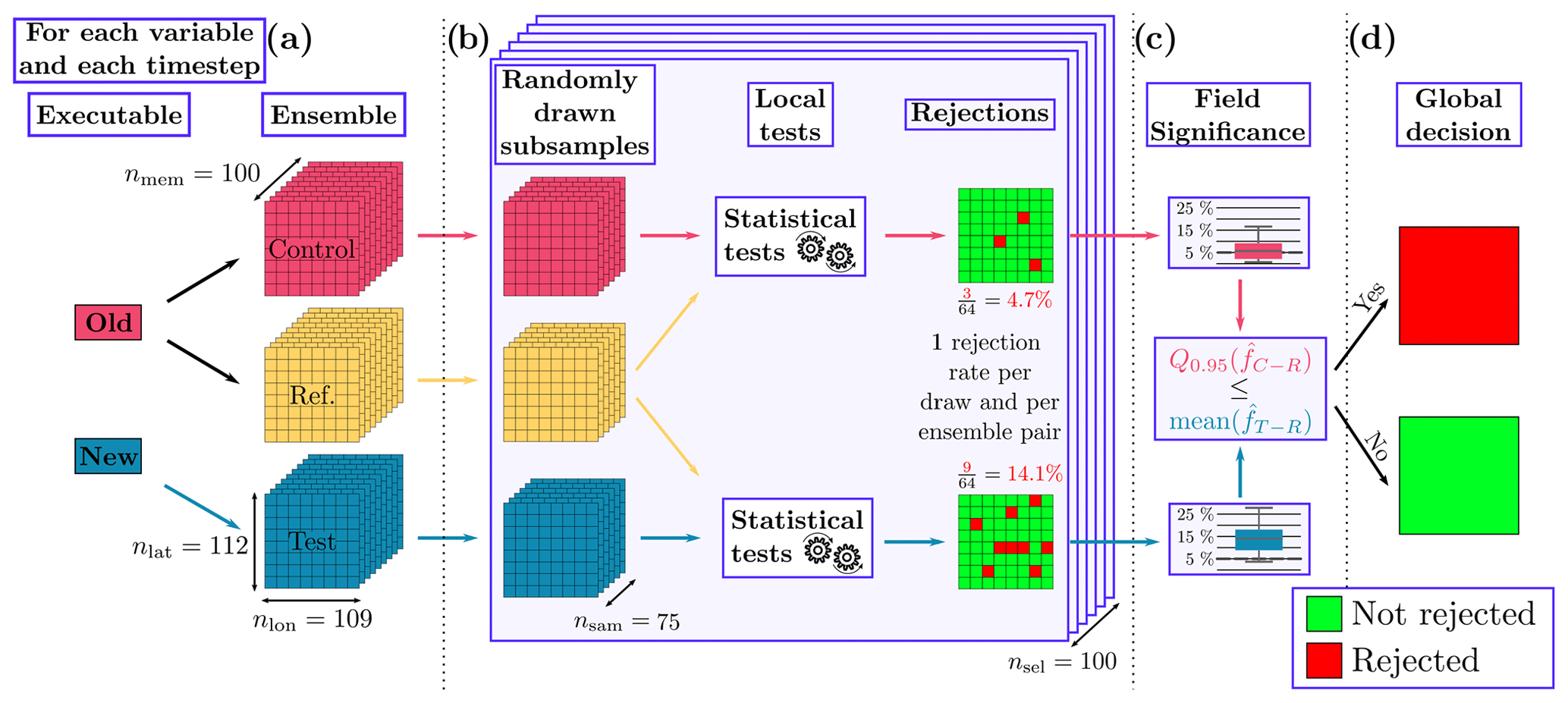
Figure 1Workflow of the statistical test. (a) Control and reference ensembles are produced by an old model, and a test ensemble is produced by a new model. (b) Subsequently, subsamples from each of the ensembles are drawn, and a statistical test is performed at each grid point of each subsample. The two resulting arrays of local rejections are then averaged into a global rejection rate. (c) The rejection rates from each subsampling step then form the two empirical distribution functions and . We compare the 95th percentile of against the mean . (d) If the mean is larger, the global null hypothesis is rejected.
2.2 Data
The methodology is applied to daily and 12-hourly output from 10-year-long regional climate simulations with the COSMO 6.0 model. These simulations are conducted on hybrid GPU–CPU nodes on the supercomputer Piz Daint operated by the Swiss National Supercomputing Centre (CSCS). The experimental setup follows the configuration of the EURO-CORDEX EUR44 experiments (Sørland et al., 2021), which employ a long–lat grid consisting of 129×132 points over a European domain with a rotated pole to ensure uniform grid spacing of 0.44° (∼50 km). The simulations are driven by boundary conditions derived from the ERA-Interim reanalysis (Dee et al., 2011). The outermost 10 grid points, identified as the nudging zone, are not considered in the analysis.
In total, seven ensemble simulations of 100 members each are performed. The ensembles are created by adding random perturbations to the initial conditions of seven prognostic variables: the three wind components, pressure, temperature, specific humidity, and cloud water content. The perturbations take the form , where φp and φ respectively represent the perturbed and unperturbed variables, R denotes a random number between −1 and 1, and ε is a small value (here ). Only initial conditions are perturbed. The lateral and upper boundary conditions are the same across all members and ensembles. This expensive total of 7000 simulated years is only necessary to assess the performance of our methodology and only feasible thanks to the relatively low grid resolution we use. The “Summary and discussion” section provides readers with recommendations to check the performance of their SP implementation in a far cheaper way.
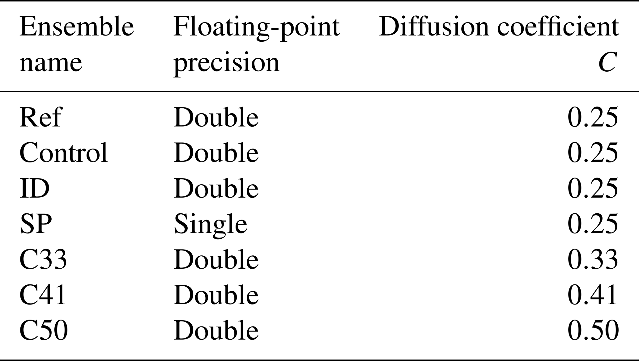
Out of the seven ensembles, three are created with parameters considered to be “default”. Two of these ensembles serve as the control and reference ensembles required by the methodology described in the previous section, while the third constitutes an identical test ensemble where every rejection is essentially a false positive. A fourth ensemble uses SP instead of the default DP and constitutes the main test. Finally, the sensitivity and performance of the methodology are evaluated using three additional ensembles using DP floats but different horizontal diffusion coefficients. These diffusion coefficients correspond to values of C=0.33, C=0.41, and C=0.50, whereas the default value is C=0.25. While increased diffusion will have a significant effect on the model behavior (Zeman et al., 2021), the magnitude of the changes above is small and lies within the range used for model tuning (Schättler et al., 2021). The previous paragraph is summarized in Table 1.
Table 1Summary of the seven ensembles created with the changes differentiating them. All other parameters are the same across all ensembles.
Our results consist of a Boolean decision time series for each of the 47 variables tested across five different test ensembles: the identity test (ID), the reduced-precision test (SP), and the modified diffusion tests with varying coefficients (C33, C41, and C50). These time series, with resolutions corresponding to the output variables, indicate whether the test was rejected (true) or passed (false).
A visual representation of our results is provided in Fig. 2, displaying monthly averaged decision time series for a representative set of 10 variables across all test ensembles. Within an individual test ensemble, the results were similar for all tested variables, typically rejecting or passing in unison. This uniformity across variables is not surprising, given the strong coupling by the governing equations. Note that this consistency remains true for the full set of 47 variables tested, except for soil variables and the surface snow amount. Those exhibited a unique pattern, characterized by more persistent and occasionally time-lagged rejections compared to their atmospheric counterparts.
The ID ensemble serves as a baseline and exhibits the fewest rejected time steps, while the number of rejected time steps increases progressively through the modified diffusion ensembles, peaking in the C50 test. Meanwhile, our primary test ensemble, SP, exhibits a low rate of rejected time steps for all variables, comparable to the ID ensemble.
Temporal trends in the rejection rates were largely absent across all ensembles, although an initial spike in rejected time steps occurred within the first 10 to 20 d of the SP simulations. This initial spike is consistent with findings from Zeman and Schär (2022) and can likely be attributed to the lower internal variability at the beginning of the simulations, making the test more sensitive to differences. Figure 3 offers a time-averaged summary for all 47 variables, illustrating a gradually increasing rate of rejected time steps from the ID ensemble to the modified diffusion tests. The ID results indicate that we can expect a false rate of rejected time steps of 10 % to 20 % for most variables. Such a high rate of false positives is likely the result of the high internal variability, probably undersampled by only 100 members, of instantaneous or 12- or 24-hourly output fields at a grid-cell level for such long simulations. For example, synoptic- or lower-scale events appearing or being stronger in some members than in others creates a lot of random noise. The average rate of rejected time steps is almost always 2 to 5 percentage points higher for SP, and we see a steady increase from ∼40 %–60 % to 100 % for the modified diffusion experiments.
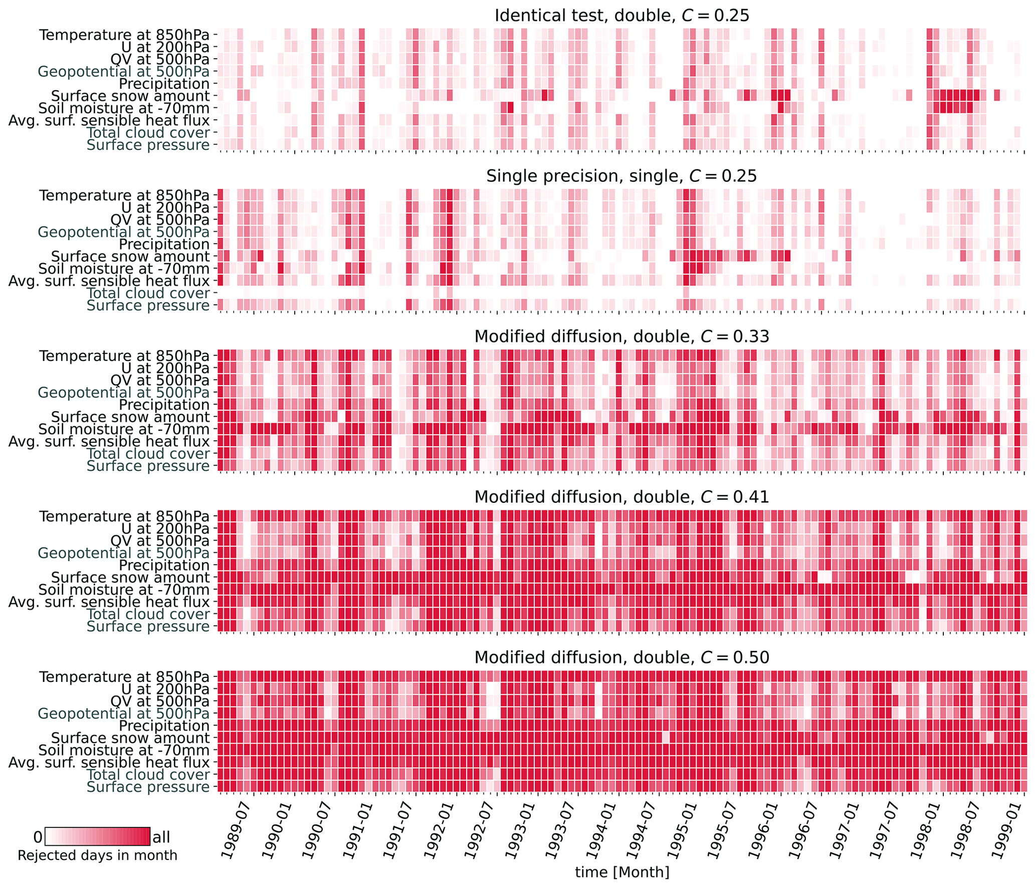
Figure 2Monthly averaged test decisions for all five test ensembles and a representative subset of 10 variables out of 47. Variables in black are output daily, while those in gray are output 12-hourly.
In the SP ensemble, five variables have a much lower rate of rejected time steps than the rest: the four cloud cover variables and the deepest soil moisture metric. This is the direct effect of the rounding applied to the data before the testing. Rounding to the fifth decimal point was used as a measure for the problem illustrated in detail in Appendix C, where those five variables exhibited an anomalously high number of rejected grid points even though the distributions were extremely similar, and coupled variables like soil temperature or precipitation showed neither such high rejection rates nor final rates of rejected time steps. To explain the issue, we take the example of total cloud cover (clct). The cause of this problem could never be elucidated, but its direct consequence is that the DP model outputs values of clct between a number close to and exactly 1, while the SP model outputs values between exactly 0 and a number close to 1–5 . This mirrored situation suggests that a part of the COSMO code adds small numbers to values at 0 and 1 to avoid those numbers, but some of it got lost in the output, which is in SP for all ensembles. These numbers do not quite correspond to machine epsilon, at least not for the SP model. While a similar issue might also exist for other variables, it is problematic for cloud cover in particular, since most grid points have a value of 0 or 1. For deep soil moisture, most grid points are at or close to 0. The KS tests, but also many rank-based tests, have spurious interactions with near ties, in which one distribution spikes at x and the other one at x±ε, where ε is a very small number. This is illustrated as the difference between Figs. C1 and C2.
In summary, these near ties can be considered artifacts of the testing methodology rather than reflecting genuine model differences, which is why we chose to use the coarse solution of rounding to the fifth decimal point to get rid of them. The results without rounding can be seen in the top row of Fig. A1.
However, for the height of the planetary boundary layer (HBL), the KS test artifact argument cannot be used, suggesting that the elevated rate of rejected time steps signals an underlying issue in the code. This highlights two key points. First, the identification potentially reveals code that is still sensitive to rounding errors in algorithms whether easy to fix (e.g., a bug) or not, thereby showcasing the effectiveness of our proposed testing method.
Second, it is worth reiterating that HBL is a purely diagnostic output variable in the COSMO model, so any imprecisions associated with it do not feed back into the subsequent model development. Nevertheless, the revealed differences in the HBL between DP and SP necessitate further analysis and likely some adaptation of the corresponding source code.
Finally, it is worth noting that the radiation and soil model are run in DP even in SP simulations, as running these components in their current state in SP causes errors that are too large. Surprisingly, variables linked to these modules still showed a slightly higher rejection rate in SP compared to ID, reflecting the coupling with the model components converted to SP.
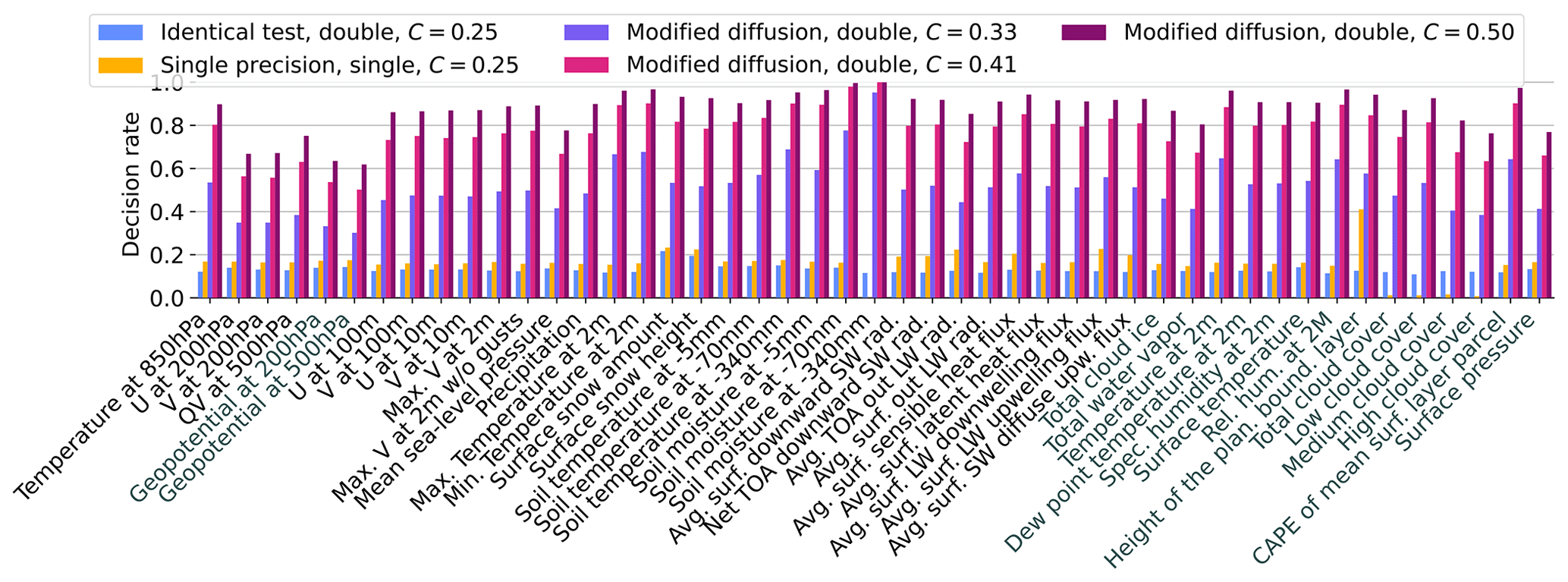
Figure 3Time-averaged test decisions for all variables and all test ensembles considered in the study. Variables in black are output daily, while those in gray are output 12-hourly.
Our results indicate that the methodology developed by Zeman and Schär (2022) is well-suited to climate simulations without requiring any modifications. It detects small changes in model parameters over long timescales while maintaining a reasonably low false rejection rate. Notably, when applied to the output of SP climate simulations, the methodology demonstrates that these simulations are comparable in quality to DP simulations during a 10-year period. The poor performance of the SP model for five variables is shown to be caused by technical artifacts rather than a significant difference between the SP and DP model results. However, a sixth variable, the height of the boundary layer, also shows poorer performance than the rest; this cannot be attributed to the same artifacts but rather to a small bug in the code, which necessitates further analysis.
However, even this significant change in the height of the boundary layer due to the use of SP comfortably lies within the variability of model results induced by the use of different model parameters as part of model tuning. Therefore, our results encourage exploiting the reduction of computational costs of around 30 % obtained from reduced precision for regional climate simulations with COSMO. More generally, the results also encourage development towards the use of reduced precision in other climate models.
To our knowledge, this work is the first to test the accuracy of reduced-precision regional climate simulations on a comprehensive set of output variables using a state-of-the-art regional climate model.
It is important to acknowledge that the tests conducted in this study were based on regional and not global climate simulations. In this type of simulation, the spread, or amount of internal variability, is inherently constrained by the lateral boundary conditions, which are exactly the same across the ensemble members. Nevertheless, the results of our sensitivity tests reveal that even in the presence of boundary forcing, we are still able to detect differences within the domain caused by relatively minor changes to the model parameters. Nonetheless, it would be valuable to extend the application of this methodology to global simulations to evaluate its performance under those conditions as well. As the methodology works with any gridded field, it is directly applicable to the output of global climate models.
Future users of the methodology developing their own SP implementation will not need to perform simulations as long and costly as done in this work in order to test it. Simulations of a few days, as done in Zeman and Schär (2022), are long enough to test the dynamics and fast atmospheric processes. We therefore recommend running those as a first verification step. Additionally, we recommend running the model with a coarse resolution like the one used in this work or even coarser for the tests, as switching off parameterization modules also means that this part of the code will not be tested for differences, and to save computational resources.
Slower processes, including, in our case, soil and snow processes – but that may also include sea ice, ocean, or atmospheric chemistry processes in a fully coupled global climate model – will need longer simulations. While a year is likely a safe choice for these processes, month-long simulations in both the cold and hot seasons would likely suffice to detect any major issues if the simulation costs are very high.
We recommend comparing the results of the main test (here, SP) against an “anti-control” test produced by changing a model parameter slightly within its tuning range, as we did with the modified diffusion ensembles C33, C41, and C50. An idea that deserves to be explored further is the use of different parameters for different timescales or processes being focused on, like the soil hydraulic conductivity for soil processes. Furthermore, many of the results shown in this work could already be observed when working with ensembles of only 10 members each, but with typically less sensitivity. The effects of reduced ensemble and subsample sizes are explored more in Zeman and Schär (2022).
We hope that our methodology makes it easier for researchers to create and verify SP implementations of the models they are creating, which is a switch our results highly encourage. Our methodology can be used on relatively short and inexpensive simulations first before moving on to longer ones depending on the stage of development of the new implementation and on the physical processes being tested. It is good to keep in mind that our methodology provides per-variable, per-output-step results and does not directly give an overall statement about the model. It is up to the user to decide what differences between the new and old implementation are acceptable, a decision that we believe is made easier when an anti-control ensemble is tested in parallel to the main test.
A commonly used approach to determine the rejection of a global null hypothesis based on the rejections of local null hypotheses is the Benjamini–Hochberg procedure (Benjamini and Hochberg, 1995), which is also known as the false discovery rate (FDR) method. It has been extensively discussed by Wilks (2016). It is highly regarded within the scientific community and may offer a cost-effective alternative to our methodology, as it does not require a control ensemble or multiple subsampling steps. Comparing the results of the two methods, we observe that most output variables exhibit similar behavior (Fig. A1). Note that, contrary to the main text figures, this figure shows the results from our methodology with no rounding applied to the variables before testing and can serve as a comparison. Certain variables however, particularly those related to radiation, demonstrate a significantly higher or lower rejection rate in the SP ensembles. Further examination reveals that these variables consistently exhibit clusters of unusually large rejections in specific regions, such as the western Sahara (not shown). We could not find an explanation for this behavior and further investigation, while certainly interesting, would be beyond the scope of this work. Confusingly, the radiation module operates using DP floats in all models, and no other related variable displays the same behavior in the regions of high rejections for the radiation variables. The presence of these large spurious rejections leads to a higher number of rejected output steps under the FDR method compared to ours. Consequently, we believe that this method is overly sensitive to outlier grid points and may be less suitable for our specific case.
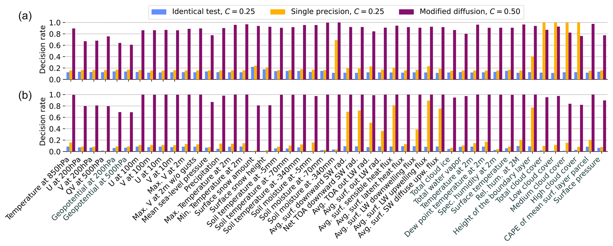
Figure A1Comparison between our method (a), but with no rounding, and the Benjamini–Hochberg procedure (b). Variables in black are output daily, while those in gray are output 12-hourly.
We now explore the effect of a coarser temporal resolution on the results presented in the main text by temporally averaging the data before applying our methodology. As a proof of concept, Fig. B1 shows the results for a single 2D field, temperature at the 850 hPa level, and a single year at the end of our simulations for six decreasing temporal resolutions. As expected, the finer temporal structure of the results erodes with decreasing temporal resolution, but the main features are there even if the data are averaged over the whole year. Interestingly, the sensitivity of the test for ID and SP is reduced with decreasing temporal resolution. Generally, we see fewer false positives with time averaging, which might be a result of the decreased internal variability coming from time averaging. However, time averaging also leads to a lower number of statistical tests performed for the same time period, which naturally leads to a lower number of false positives. Therefore, the relatively smooth rejection curves for the time-averaged results might be a bit misleading. For example, for the 1-year average, only one decision is made, naturally leading to a straight line in this diagram. Nevertheless, time coarsening may prove to be a valuable path forward if one is not interested in the fine-grained details in the temporal distribution of the rejections or the model's representation of extreme events.
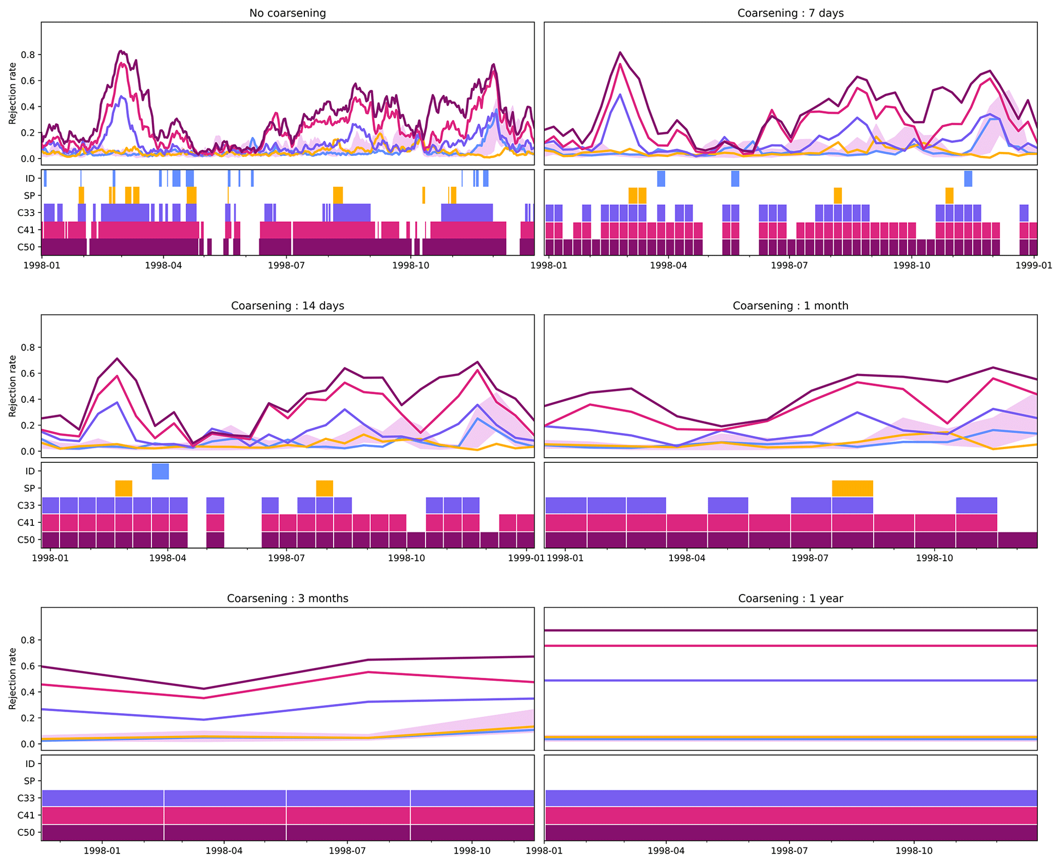
Figure B1Rejection rate and associated decision (colored box: reject) for different magnitudes of time coarsening and/or averaging of temperature at 850 hPa for 1 year of output data.
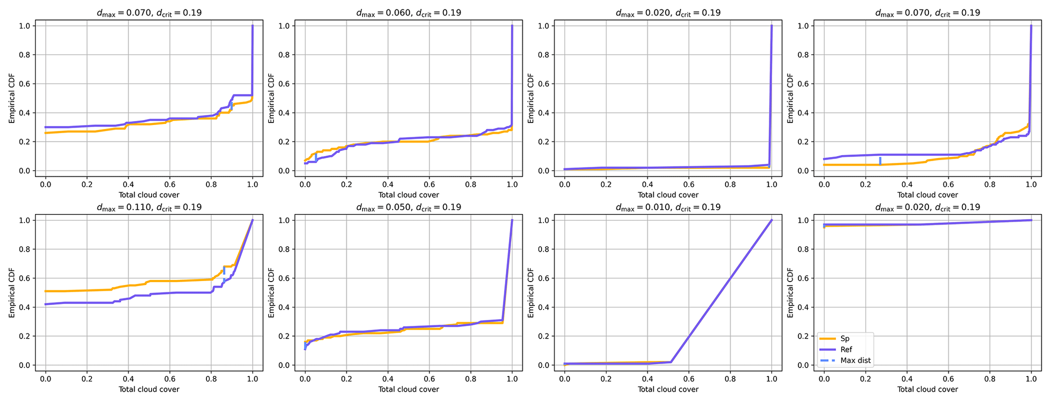
In the Results section of the main text, we found six variables to have large decision rates for the SP ensemble, which seemed at odds with the fact that all other coupled variables (e.g., precipitation) showed low decision rates. To investigate this issue, we perform the first step of our methodology and apply the KS test to the ensemble distribution of randomly chosen grid points and output time steps, and we show the results for eight of them in Fig. C1. The dashed blue line represents the largest vertical distance between the empirical distribution and the x position at which it is found. This maximum vertical distance is this test's statistic, which is then compared against a rejection threshold for the null hypothesis. Figure C1 shows that this maximum distance is always found at points where both distributions have a large positive derivative before reaching 1 and where both lines seem to overlap. The issue is that the lines do not actually overlap but rather reach a different number. One reaches 1, and the other reaches 1−ε, where ε is small number . The mirrored situation between 0 and ε also happens. This is sufficient to create a large vertical distance between the two distributions at . We confirm this by rounding the variable to the fourth decimal for both ensembles and observe in Fig. C2 that none of these days are rejected with this added rounding.
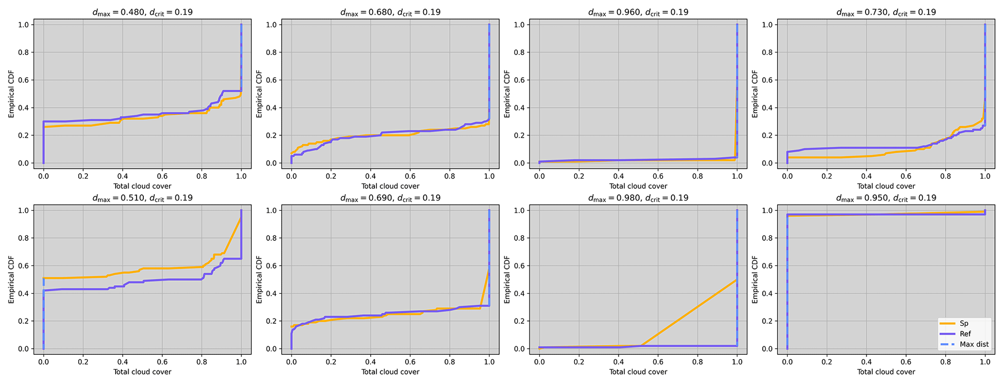
Figure C1Example KS results for total cloud cover for 8 random days without rounding. The gray background indicates that all these results lead to a local rejection.
The code for the data analysis presented in this work is available at https://doi.org/10.5281/zenodo.8398547 (Banderier, 2023b). COSMO may be used for operational and research applications by the members of the COSMO consortium. Moreover, within a license agreement, the COSMO model may be used for operational and research applications by other national (hydro)meteorological services, universities, and research institutes.
The model is driven by boundary conditions extracted from the ERA-Interim dataset, which is publicly available. The input parameters for COSMO can be found in the repository where the rest of the code is located. The COSMO output data are over 10 TB so they cannot be hosted online, but they can be made available upon request. Spatially averaged test results as well as final decisions of the methodology are published at https://doi.org/10.5281/zenodo.8399468 (Banderier, 2023a).
HB and CZ designed the study. HB performed the ensemble simulations, wrote the code for the verification (based on Zeman and Schär, 2022), and performed the verification and analysis of the model results with input from CZ and DL. All authors were involved in the discussion of the results. HB and CZ wrote the paper with strong contributions and review from all other co-authors.
The contact author has declared that none of the authors has any competing interests.
Publisher's note: Copernicus Publications remains neutral with regard to jurisdictional claims made in the text, published maps, institutional affiliations, or any other geographical representation in this paper. While Copernicus Publications makes every effort to include appropriate place names, the final responsibility lies with the authors.
We acknowledge PRACE for awarding computational resources for the COSMO simulations on Piz Daint at the Swiss National Supercomputing Centre (CSCS). We also acknowledge the Federal Office for Meteorology and Climatology MeteoSwiss, CSCS, and ETH Zurich for their contributions to the development of the GPU-accelerated version of COSMO with single-precision capability.
This paper was edited by James Kelly and reviewed by Milan Klöwer and one anonymous referee.
Ackmann, J., Dueben, P. D., Palmer, T., and Smolarkiewicz, P. K.: Mixed-Precision for Linear Solvers in Global Geophysical Flows, J. Adv. Model. Earth Sy., 14, e2022MS003148, https://doi.org/10.1029/2022MS003148, 2022. a
Banderier, H.: Spatially averaged test results comparing SP and DP COSMO simulations, Zenodo [data set], https://doi.org/10.5281/zenodo.8399468, 2023a. a
Banderier, H.: hbanderier/cosmo-sp: v1.0.0-rc.1, Zenodo [code], https://doi.org/10.5281/zenodo.8398547, 2023b. a
Benjamini, Y. and Hochberg, Y.: Controlling the False Discovery Rate: A Practical and Powerful Approach to Multiple Testing, J. Roy. Stat. Soc. B Met., 57, 289–300, https://doi.org/10.1111/j.2517-6161.1995.tb02031.x, 1995. a
Brown, A., Milton, S., Cullen, M., Golding, B., Mitchell, J., and Shelly, A.: Unified Modeling and Prediction of Weather and Climate: A 25-Year Journey, B. Am. Meteorol. Soc., 93, 1865–1877, https://doi.org/10.1175/BAMS-D-12-00018.1, 2012. a
Chantry, M., Thornes, T., Palmer, T., and Düben, P.: Scale-Selective Precision for Weather and Climate Forecasting, Mon. Weather Rev., 147, 645–655, https://doi.org/10.1175/MWR-D-18-0308.1, 2019. a, b, c
Croci, M., Fasi, M., Higham, N. J., Mary, T., and Mikaitis, M.: Stochastic rounding: implementation, error analysis and applications, Roy. Soc. Open Sci., 9, 211631, https://doi.org/10.1098/rsos.211631, 2022. a
Dee, D. P., Uppala, S. M., Simmons, A. J., Berrisford, P., Poli, P., Kobayashi, S., Andrae, U., Balmaseda, M. A., Balsamo, G., Bauer, P., Bechtold, P., Beljaars, A. C. M., van de Berg, L., Bidlot, J., Bormann, N., Delsol, C., Dragani, R., Fuentes, M., Geer, A. J., Haimberger, L., Healy, S. B., Hersbach, H., Hólm, E. V., Isaksen, L., Kållberg, P., Köhler, M., Matricardi, M., McNally, A. P., Monge-Sanz, B. M., Morcrette, J.-J., Park, B.-K., Peubey, C., de Rosnay, P., Tavolato, C., Thépaut, J.-N., and Vitart, F.: The ERA-Interim reanalysis: configuration and performance of the data assimilation system, Q. J. Roy. Meteor. Soc., 137, 553–597, https://doi.org/10.1002/qj.828, 2011. a
Düben, P. D. and Palmer, T. N.: Benchmark Tests for Numerical Weather Forecasts on Inexact Hardware, Mon. Weather Rev., 142, 3809–3829, https://doi.org/10.1175/MWR-D-14-00110.1, 2014. a
ECMWF: IFS documentation CY48R1 – part III: Dynamics and numerical procedures, in: IFS Documentation CY48R1, ECMWF, https://doi.org/10.21957/26f0ad3473, 2023. a
Geer, A.: Significance of changes in medium-range forecast scores, ECMWF, https://www.ecmwf.int/en/elibrary/78783-significance-changes-medium-range-forecast-scores (last access: 2 June 2023), 2015. a
Gustafson, J. L. and Yonemoto, I. T.: Beating Floating Point at its Own Game: Posit Arithmetic, Supercomputing Frontiers and Innovations, 4, 71–86, https://doi.org/10.14529/jsfi170206, 2017. a
Jablonowski, C. and Williamson, D. L.: A baroclinic instability test case for atmospheric model dynamical cores, Q. J. Roy. Meteor. Soc., 132, 2943–2975, https://doi.org/10.1256/qj.06.12, 2006. a
Kimpson, T., Paxton, E. A., Chantry, M., and Palmer, T.: Climate-change modelling at reduced floating-point precision with stochastic rounding, Q. J. Roy. Meteor. Soc., 149, 843–855, https://doi.org/10.1002/qj.4435, 2023. a, b, c
Klöwer, M., Düben, P. D., and Palmer, T. N.: Number Formats, Error Mitigation, and Scope for 16-Bit Arithmetics in Weather and Climate Modeling Analyzed With a Shallow Water Model, J. Adv. Model. Earth Sy., 12, e2020MS002246, https://doi.org/10.1029/2020MS002246, 2020. a
Kucharski, F., Molteni, F., and Bracco, A.: Decadal interactions between the western tropical Pacific and the North Atlantic Oscillation, Clim. Dynam., 26, 79–91, https://doi.org/10.1007/s00382-005-0085-5, 2006. a
Kucharski, F., Molteni, F., King, M. P., Farneti, R., Kang, I.-S., and Feudale, L.: On the Need of Intermediate Complexity General Circulation Models: A “SPEEDY” Example, B. Am. Meteorol. Soc., 94, 25–30, https://doi.org/10.1175/BAMS-D-11-00238.1, 2013. a
Lang, S. T. K., Dawson, A., Diamantakis, M., Dueben, P., Hatfield, S., Leutbecher, M., Palmer, T., Prates, F., Roberts, C. D., Sandu, I., and Wedi, N.: More accuracy with less precision, Q. J. Roy. Meteor. Soc., 147, 4358–4370, https://doi.org/10.1002/qj.4181, 2021. a, b
Manabe, S. and Wetherald, R. T.: Thermal Equilibrium of the Atmosphere with a Given Distribution of Relative Humidity, J. Atmos. Sci., 24, 241–259, https://doi.org/10.1175/1520-0469(1967)024<0241:TEOTAW>2.0.CO;2, 1967. a
Matheson, J. E. and Winkler, R. L.: Scoring Rules for Continuous Probability Distributions, Manage. Sci., 22, 1087–1096, https://doi.org/10.1287/mnsc.22.10.1087, 1976. a
Maynard, C. M. and Walters, D. N.: Mixed-precision arithmetic in the ENDGame dynamical core of the Unified Model, a numerical weather prediction and climate model code, Comput. Phys. Commun., 244, 69–75, https://doi.org/10.1016/j.cpc.2019.07.002, 2019. a
Molteni, F.: Atmospheric simulations using a GCM with simplified physical parametrizations. I: model climatology and variability in multi-decadal experiments, Clim. Dynam., 20, 175–191, https://doi.org/10.1007/s00382-002-0268-2, 2003. a
Nakano, M., Yashiro, H., Kodama, C., and Tomita, H.: Single Precision in the Dynamical Core of a Nonhydrostatic Global Atmospheric Model: Evaluation Using a Baroclinic Wave Test Case, Mon. Weather Rev., 146, 409–416, https://doi.org/10.1175/MWR-D-17-0257.1, 2018. a
Paxton, E. A., Chantry, M., Klöwer, M., Saffin, L., and Palmer, T.: Climate Modeling in Low Precision: Effects of Both Deterministic and Stochastic Rounding, J. Climate, 35, 1215–1229, https://doi.org/10.1175/JCLI-D-21-0343.1, 2022. a, b, c, d
Rüdisühli, S., Walser, A., and Fuhrer, O.: Cosmo in single precision, COSMO Newsletter, http://www.cosmo-model.org/content/model/documentation/newsLetters/newsLetter14/cnl14_09.pdf (last access: 17 May 2023), 2014. a, b, c, d
Saffin, L., Hatfield, S., Düben, P., and Palmer, T.: Reduced-precision parametrization: lessons from an intermediate-complexity atmospheric model, Q. J. Roy. Meteor. Soc., 146, 1590–1607, https://doi.org/10.1002/qj.3754, 2020. a
Satoh, M., Tomita, H., Yashiro, H., Miura, H., Kodama, C., Seiki, T., Noda, A. T., Yamada, Y., Goto, D., Sawada, M., Miyoshi, T., Niwa, Y., Hara, M., Ohno, T., Iga, S.-i., Arakawa, T., Inoue, T., and Kubokawa, H.: The Non-hydrostatic Icosahedral Atmospheric Model: description and development, Progress in Earth and Planetary Science, 1, 18, https://doi.org/10.1186/s40645-014-0018-1, 2014. a
Schär, C., Fuhrer, O., Arteaga, A., Ban, N., Charpilloz, C., Girolamo, S. D., Hentgen, L., Hoefler, T., Lapillonne, X., Leutwyler, D., Osterried, K., Panosetti, D., Rüdisühli, S., Schlemmer, L., Schulthess, T. C., Sprenger, M., Ubbiali, S., and Wernli, H.: Kilometer-Scale Climate Models: Prospects and Challenges, B. Am. Meteorol. Soc., 101, E567–E587, https://doi.org/10.1175/BAMS-D-18-0167.1, 2020. a
Schättler, U., Doms, G., and Schraff, C.: A Description of the Nonhydrostatic Regional COSMO-Model – Part VII – User's Guide, Deutscher Wetterdienst, https://doi.org/10.5676/DWD_pub/nwv/cosmo-doc_6.00_VII, 2021. a
Sørland, S. L., Brogli, R., Pothapakula, P. K., Russo, E., Van de Walle, J., Ahrens, B., Anders, I., Bucchignani, E., Davin, E. L., Demory, M.-E., Dosio, A., Feldmann, H., Früh, B., Geyer, B., Keuler, K., Lee, D., Li, D., van Lipzig, N. P. M., Min, S.-K., Panitz, H.-J., Rockel, B., Schär, C., Steger, C., and Thiery, W.: COSMO-CLM regional climate simulations in the Coordinated Regional Climate Downscaling Experiment (CORDEX) framework: a review, Geosci. Model Dev., 14, 5125–5154, https://doi.org/10.5194/gmd-14-5125-2021, 2021. a, b
Váňa, F., Düben, P., Lang, S., Palmer, T., Leutbecher, M., Salmond, D., and Carver, G.: Single Precision in Weather Forecasting Models: An Evaluation with the IFS, Mon. Weather Rev., 145, 495–502, https://doi.org/10.1175/MWR-D-16-0228.1, 2017. a, b
Wilks, D. S.: “The Stippling Shows Statistically Significant Grid Points”: How Research Results are Routinely Overstated and Overinterpreted, and What to Do about It, B. Am. Meteorol. Soc., 97, 2263–2273, https://doi.org/10.1175/BAMS-D-15-00267.1, 2016. a, b
Zeman, C. and Schär, C.: An ensemble-based statistical methodology to detect differences in weather and climate model executables, Geosci. Model Dev., 15, 3183–3203, https://doi.org/10.5194/gmd-15-3183-2022, 2022. a, b, c, d, e, f, g, h, i, j, k
Zeman, C., Wedi, N. P., Dueben, P. D., Ban, N., and Schär, C.: Model intercomparison of COSMO 5.0 and IFS 45r1 at kilometer-scale grid spacing, Geosci. Model Dev., 14, 4617–4639, https://doi.org/10.5194/gmd-14-4617-2021, 2021. a
- Abstract
- Introduction
- Methods and data
- Results
- Summary and discussion
- Appendix A: Comparison with the Benjamini–Hochberg procedure
- Appendix B: Time coarsening
- Appendix C: Cloud cover and rounding problem
- Code availability
- Data availability
- Author contributions
- Competing interests
- Disclaimer
- Acknowledgements
- Review statement
- References