the Creative Commons Attribution 4.0 License.
the Creative Commons Attribution 4.0 License.
 | 27 Jun 2024
WRF-Comfort: simulating microscale variability in outdoor heat stress at the city scale with a mesoscale model
Alberto Martilli
Negin Nazarian
E. Scott Krayenhoff
Jacob Lachapelle
Jiachen Lu
Esther Rivas
Alejandro Rodriguez-Sanchez
Beatriz Sanchez
José Luis Santiago
Urban overheating and its ongoing exacerbation due to global warming and urban development lead to increased exposure to urban heat and increased thermal discomfort and heat stress. To quantify thermal stress, specific indices have been proposed that depend on air temperature, mean radiant temperature (MRT), wind speed, and relative humidity. While temperature and humidity vary on scales of hundreds of meters, MRT and wind speed are strongly affected by individual buildings and trees and vary on the meter scale. Therefore, most numerical thermal comfort studies apply microscale models to limited spatial domains (commonly representing urban neighborhoods with building blocks) with resolutions on the order of 1 m and a few hours of simulation. This prevents the analysis of the impact of city-scale adaptation and/or mitigation strategies on thermal stress and comfort. To solve this problem, we develop a methodology to estimate thermal stress indicators and their subgrid variability in mesoscale models – here applied to the multilayer urban canopy parameterization BEP-BEM within the Weather Research and Forecasting (WRF) model. The new scheme (consisting of three main steps) can readily assess intra-neighborhood-scale heat stress distributions across whole cities and for timescales of minutes to years. The first key component of the approach is the estimation of MRT in several locations within streets for different street orientations. Second, mean wind speed and its subgrid variability are downscaled as a function of the local urban morphology based on relations derived from a set of microscale LES and RANS simulations across a wide range of realistic and idealized urban morphologies. Lastly, we compute the distributions of two thermal stress indices for each grid square, combining all the subgrid values of MRT, wind speed, air temperature, and absolute humidity. From these distributions, we quantify the high and low tails of the heat stress distribution in each grid square across the city, representing the thermal diversity experienced in street canyons. In this contribution, we present the core methodology as well as simulation results for Madrid (Spain), which illustrate strong differences between heat stress indices and common heat metrics like air or surface temperature both across the city and over the diurnal cycle.
- Article
(10012 KB) - Full-text XML
- BibTeX
- EndNote


The combination of urban development and climate change has increased heat exposure in cities in recent decades (Tuholske et al., 2021), and a continuation of these trends in the 21st century would be difficult to offset locally from an air temperature perspective (Broadbent et al., 2020; Krayenhoff et al., 2018; Zhao et al., 2021). Adaptation options that target contributions to heat exposure other than the air temperature, such as radiation (e.g., via shade) and wind (e.g., via improved street ventilation), should therefore be considered. The quantification of these contributions relative to air temperature requires the application of comprehensive thermophysiological heat stress metrics such as the universal thermal climate index, UTCI (Jendritzky et al., 2012); the physiological equivalent temperature, PET (Höppe, 1999); or the standard effective temperature, SET (Gagge et al., 1986). Moreover, exposure to heat hazards is moderated by infrastructure-based and social/mobility-based adaptations to heat and by buildings and associated cooling mechanisms. Here, the focus is the development of a tool to quantify the outdoor component of heat exposure in cities, accounting for all relevant meteorological variables.
Heat exposure in urban areas is affected by several meteorological variables that vary on different spatial and temporal scales (Nazarian et al., 2022). While temperature and humidity vary on spatial scales on the order of hundreds of meters, shortwave and longwave radiation and wind speed are strongly affected by individual buildings and vary on the scale of a few meters. For this reason, most numerical thermal comfort studies in urban areas apply microscale models with resolutions on the order of 1 m and spatial domains that are limited to an urban block or neighborhood (Nazarian et al., 2017; Zhang et al., 2022; Geletič et al., 2018). While these studies include substantial detail on the microscale, they are computationally very expensive and therefore can only be applied to a few neighborhoods, and they neglect the interactions with larger-scale meteorological phenomena (e.g., land/sea breezes, mountain/valley winds, and urban breezes) that often play a relevant role in outdoor thermal comfort and its variation across cities. On the other hand, contemporary mesoscale numerical models can be applied to the whole urban area and surrounding regions and therefore capture these larger-scale phenomena but have spatial resolutions of several hundred meters at best. These models use a grid mesh that does not resolve buildings and is therefore too coarse to capture the fine-scale variation in radiation and wind flow of relevance to outdoor heat exposure and ultimately thermal comfort.
The objective of this work is to fill the aforementioned gap by developing a model that includes the most crucial capabilities of microscale assessments of thermal exposure within mesoscale models. This new model will quantify the spatial variability (i.e., statistical representation of the microscale distribution) for longwave and shortwave radiation as well as wind speed within each mesoscale grid square. Subsequently, it will capture the range of thermal exposure, as quantified by the UTCI and SET thermal stress metrics, within each urban grid square across a city at each time of day. The focus here is on the range of thermal exposure, such that we identify the cool and hot spots within the grid cell without having to resolve the entire spatial distribution. We argue that this represents the most crucial information for heat management and urban design interventions as it identifies whether people can move and search for optimal thermal conditions. For example, if hot spots are experiencing extreme heat stress but the cool spots are at slight heat stress, pedestrians have the opportunity and autonomy to seek shade and thermal respite (i.e., temporal and spatial autonomy as described in Nazarian et al., 2019). Conversely, if the conditions in the cool spot are already in extreme heat stress, this can be used to inform urban design interventions or heat advisories to vulnerable populations to avoid being outside at that place and time. Overall, representing the range of heat exposure on the neighborhood scale while covering regional-scale phenomena is key to human-centric assessments of urban overheating (Nazarian et al., 2022).
The new model is embedded in the multilayer urban canopy parameterization BEP-BEM (Martilli et al., 2002; Salamanca et al., 2010), which simulates the local-scale meteorological effects of the grid-average urban morphology within the Weather Research and Forecasting (WRF) mesoscale model (Skamarock et al., 2021; version 4.3 has been used in this study). Here, BEP-BEM is extended to quantify the spatial variation in the mean radiant temperature and wind speed within the grid square at the pedestrian level. To our knowledge, three schemes in the published literature have attempted to capture thermal exposure in an urban canopy model. Pigliautile et al. (2020) implemented a scheme to estimate human thermal exposure in the Princeton single-layer urban canopy model. However, the scheme has not been run within a mesoscale model. Jin et al. (2022) calculate urban mean radiant temperature (MRT) in a mesoscale model, while Lemonsu et al. (2015) and Leroyer et al. (2018) assess UTCI in mesoscale modeling applications within Paris and Toronto, respectively. Moreover, Giannaros et al. (2018, 2023) made an offline coupling of WRF–BEP-BEM with RayMan (Matzarakis et al., 2007). However, none of these approaches account for the within-grid spatial variation in wind speed, and their assessment of subgrid spatial variation in radiation exposure (i.e., mean radiant temperature) is limited. Here, we further extend the BEP-BEM model embedded in the WRF mesoscale model to overcome these limitations and better assess spatial variation in thermal exposure within each urban grid square.
In Sect. 2, the methodology is described in detail, with a focus on model development and implementation in WRF. In Sect. 3, we present an example of the type of outputs that can be produced. In Sect. 4, the limitations of the approach are discussed. Conclusions are in Sect. 5.
The most complete thermal stress indices invariably depend on four meteorological variables: air temperature, mean radiant temperature (MRT), relative humidity, and wind speed. Among these, MRT and wind speed have the largest spatial variability in the urban canopy, and this variability is often captured with 3D microscale models of urban airflow and radiative heat transfer. On the mesoscale, however, it is not feasible to incorporate such models, motivating the simplified urban canopy parameterizations developed here. Below we detail how the BEP-BEM urban canopy model is modified to (a) introduce a simplified model for MRT variation within a mesoscale grid cell (Sect. 2.1) and (b) parameterize airflow variability (Sect. 2.2) in the urban canopy within a grid cell and make a simple estimate of air temperature variability. These meteorological parameters are then used to estimate the subgrid-scale variation in thermal stress indices (Sect. 2.3), namely SET and UTCI, as two of the most commonly used indices for outdoor environments (Potchter et al., 2018). Lastly, we discuss how multi-scale temporal and spatial variabilities in thermal exposure can be effectively communicated using the outcomes of the updated WRF–BEP-BEM model.
2.1 A simplified model for MRT variability in the urban canopy
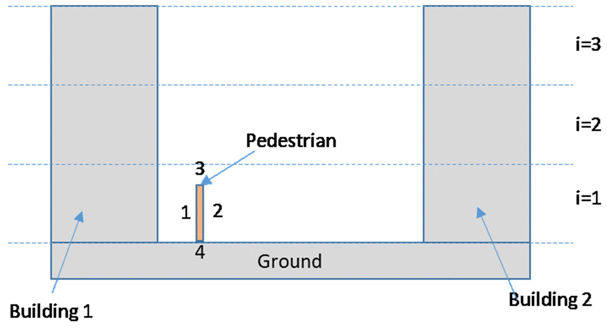
The mean radiant temperature is a measure of the total radiation flux absorbed by the human body, including both shortwave (from the sun, either directly or after reflection on the walls or road) and longwave (emitted from solid bodies like walls or road or from the sky) radiation. Whether pedestrians are shaded or in the sunshine as well as their distance from warm surfaces emitting radiation are therefore very important. BEP-BEM applies a simple urban morphology: two street canyons of different orientations, each with the same street width and building height distribution on each side of the canyon (Martilli et al., 2002). To capture the within-grid spatial extremes of mean radiant temperature, we assess pedestrian locations at the center of the street for two canyon orientations considered in BEP-BEM and at positions located at a distance of 1.5 m from the building wall on each side of the street, representing the sidewalks. Thus, there are six positions (three for each street direction) in each urban grid square where we compute the mean radiant temperature (shown for the example of north–south and east–west streets in Fig. 1). For shortwave and longwave radiation exchange, the standard BEP view factor and shading routines (Martilli et al., 2002) are used to estimate the amount of shortwave (direct and diffuse) and longwave radiation reaching a vertical segment that is 1.80 m tall and located in each of the previously mentioned six positions (Fig. 1; Appendix A). The reflection of shortwave radiation and emission and reflection of longwave radiation from both building walls and the street surface are accounted for via these view factors. The pedestrian is “transparent” from the perspective of the urban facets, meaning that its presence does not alter the shortwave and longwave radiation reaching the building walls and road. The mean radiant temperature is computed by weighting the radiation reaching each side of the vertical segment by 0.44 and the radiation reaching the downward- and upward-facing (at 1.80 m height) surfaces of the pedestrian by 0.06 each. This approach follows the six-directional weighting method (Thorsson et al., 2007) and aggregates the four lateral weightings of 0.22 into two lateral weightings of 0.44 since BEP-BEM is a two-dimensional model (e.g., the streets are considered infinitely long). Namely, the following applies:
where, for a N–S-oriented street, is for the vertical sides of the pedestrian looking east and west and is for the top and bottom, respectively. Therefore, and , while the absorptivity of the pedestrian in the shortwave and longwave, aK (the absorption coefficient for shortwave radiation of the human body) and aL (the absorption coefficient for longwave radiation, or emissivity, of the human body), respectively, are aK=0.7 and aL=0.97. K1,2 and L1,2 are the shortwave and longwave radiation reaching the vertical segment; K3,4 and L3,4 are shortwave and longwave radiation reaching the top and bottom, respectively; and σ is the Stefan–Boltzmann constant (see Appendix A for details about how the radiation components are computed).
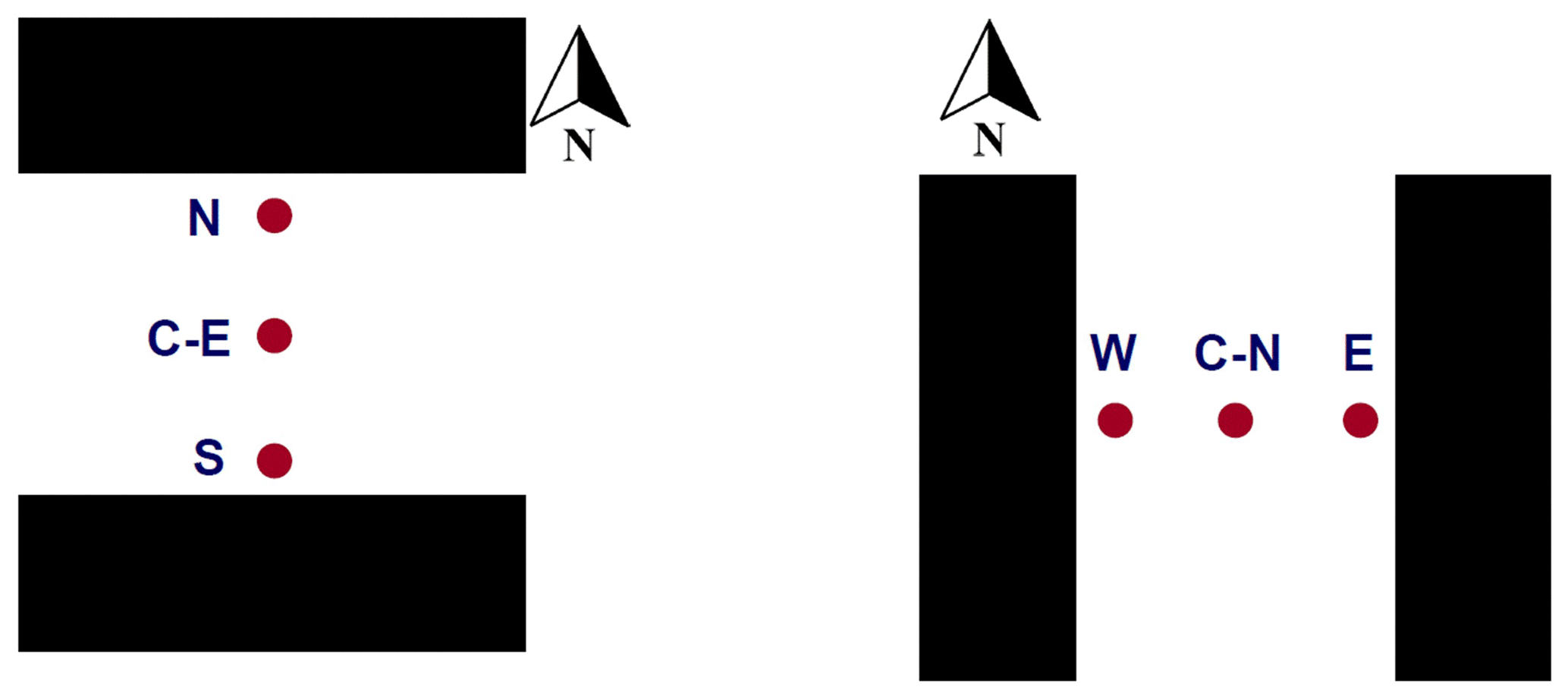
Figure 1Two street directions (E–W canyon on the left; N–S canyon on the right) and pedestrian locations considered for Mean Radiant Temperature calculations.
The diurnal progression of the mean radiant temperature computed by this new model in BEP-BEM is subsequently compared with that obtained from TUF-Pedestrian, a more detailed three-dimensional model that has been evaluated against measurements (Lachapelle et al., 2022; Jiang et al., 2023). TUF-Pedestrian is configured with identical input parameters and meteorological forcing and with long canyons that approximate the two-dimensional BEP-BEM canyon geometry. The new model clearly captures the relevant details of the diurnal progression of MRT at all six locations (Fig. 2), with a mean absolute difference of 3.4 K and a root mean square difference of 4.3 K across all locations. A comparison of the shortwave radiation loading on the pedestrian between the two models reveals very good agreement (Appendix B; Figs. B1 and B2), considering the highly simplified urban morphology used by BEP-BEM, with the biggest errors limited to short periods of time; thus, most of the model disagreement arises from differences between longwave loading on the pedestrian as a result of different methods for the computation of surface temperature between the models. Overall, the new model of mean radiation temperature in BEP-BEM provides satisfactory results.
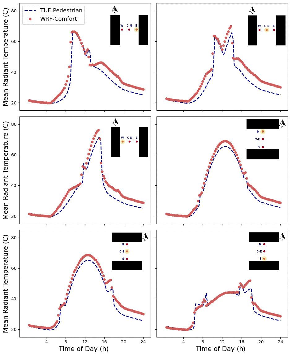
Figure 2Comparison of diurnal variation in mean radiant temperature (MRT) between the new model in BEP-BEM and TUF-Pedestrian for each of the six locations in Fig. 1. TUF pedestrian acts here as a reference.
2.2 Parameterize airflow variability in the urban canopy
Mesoscale models solve conservation equations for the three components of momentum. From these, it is possible to derive the spatially averaged wind velocity in each grid cell at the grid resolution of the mesoscale model, commonly on the order of 300 m–1 km. The spatially averaged wind velocity in the urban canopy, 〈V〉, close to the pedestrian height (∼ 2.5 m), is the square root of the sum of the spatial average of the two horizontal components, u and v (neglecting the vertical component, which is usually at least 1 or 2 orders of magnitude smaller than the horizontal):
where Vair is the volume of the grid cell occupied by air (e.g., without the buildings).
However, the wind velocity calculated in mesoscale models is different from the average wind speed that would be experienced by a person in the grid cell. This is better represented by the spatial average of the wind speed, 〈U〉 (e.g., the modulus of the vector), written as
To assess the impact of airflow on human thermal comfort, the wind speed should be estimated from the wind velocity computed in the mesoscale models. Additionally, it is critical to parameterize and estimate the spatial variability in mean wind speed in the urban canopy. Accounting for these factors, the range of wind speed variability at the pedestrian level is estimated, which is critical for the quantification of spatial variability in outdoor thermal stress and comfort.
Here, we describe the parameterization of (a) wind-speed-to-velocity ratio and (b) wind speed distribution based on urban density parameters. Data are considered from over 173 microscale computational fluid dynamics (CFD) simulations of urban airflow over realistic and idealized urban configurations, spanning a wide range of building plan area (λP), frontal area (λF), and wall area (λw) densities representative of realistic urban neighborhoods in different types of cities. CFD simulations are conducted using large-eddy simulations (LES; 162 cases) and Reynolds-averaged Navier–Stokes (RANS; 11 cases) schemes detailed in Appendix C.
Spatial averages of mean wind velocity (〈V〉) and speed (〈U〉) and its spatial standard deviation (σU) are computed at a horizontal cross section at pedestrian height for each CFD simulation and used to derive parameterizations (Fig. 3). An additional data point is added at , ensuring that wind speed is equal to wind velocity, and its standard deviation is set to zero for the non-urban case. It is important to remark here that we are dealing with the standard deviation of the spatial distribution of the mean wind speed. With the term “mean”, we indicate the result of an ensemble (over many realizations) or a time average (over timescales larger than the turbulence timescale but smaller than the timescale of the mesoscale motions) but not a spatial average. The urban canopy is, in fact, spatially heterogeneous, and, for this reason, the time and ensemble averages are different than the spatial average. Only when (e.g., there are no buildings) and the horizontal homogeneity is recovered must the variability be zero. This σU, therefore, should not be confounded with the turbulent σ, which indicates the variability in instantaneous wind speed induced by turbulent motions, which is indeed not zero even when there are no buildings.
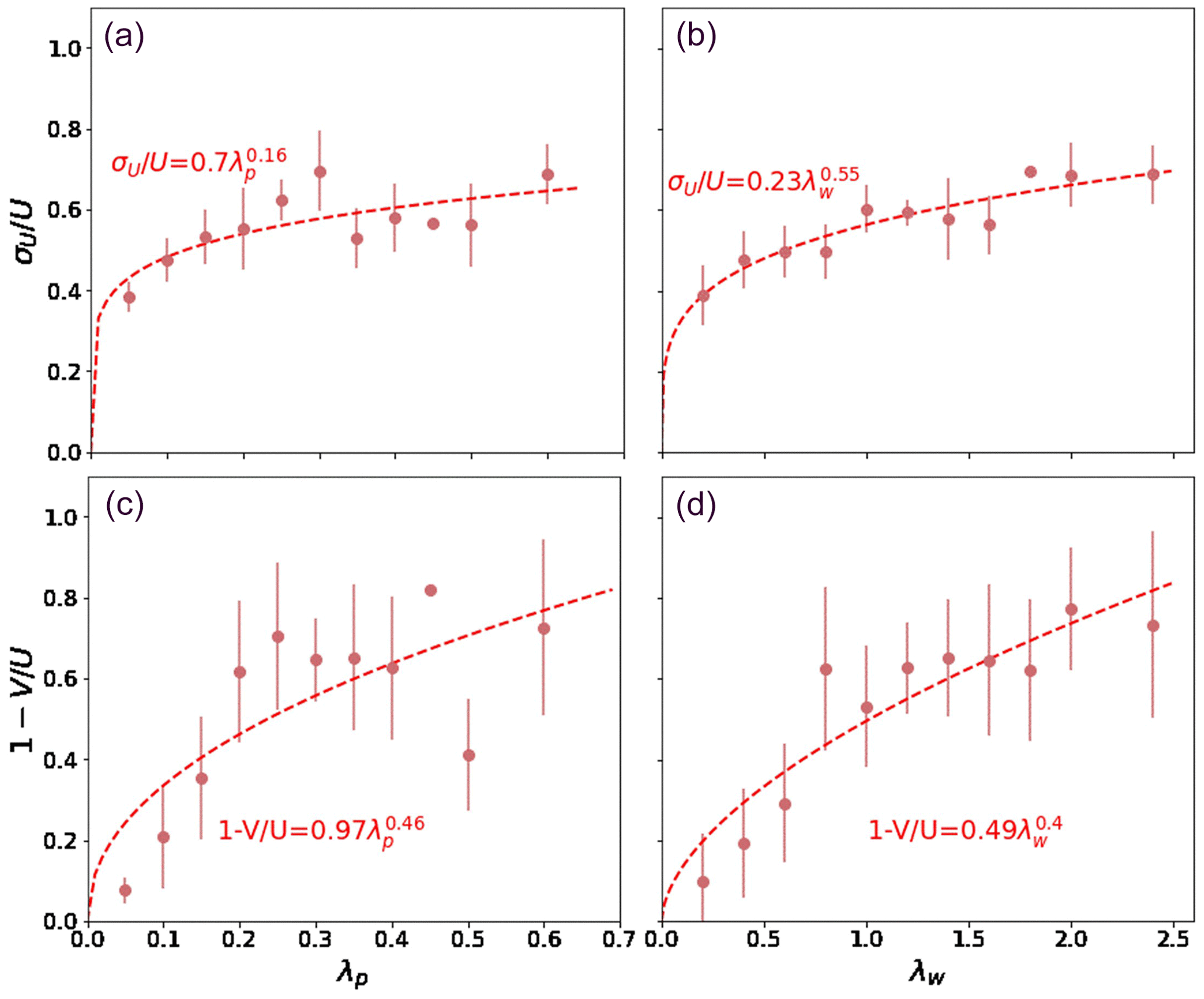
Figure 3Relationship between (c, d) and (a, b) and two morphological parameters, λP (a, c) and λw (b, d), based on the CFD simulations. Dots represent the average of the value among all the simulations that share the same morphological parameter and the vertical bar indicates the standard deviation. The dashed line and the formula indicate the best fit.
Parameterizations are derived (shown in Fig. 3) for two density parameters, ( and , where Ap is the area of the horizontal surface occupied by buildings or the roof area; Aw is the area of vertical, i.e., wall, surfaces; and Atot is the total horizontal area). We find that λw better predicts mean wind speed and its spatial variability at the pedestrian height because it represents both horizontal and vertical heterogeneities in the urban canopy. Note that λF has not been included in the study, given the difficulty of estimating it for real urban areas and to translate it to the simplified 2D urban morphology used by BEP-BEM. In any case, λF is closely related to λw. Therefore, the following parameterizations are implemented at the pedestrian height as a function of the wall area density, λw:
We, therefore, assign the following three values of wind speed in each grid cell:
Note that here we consider the three values to be equally likely in order to realistically span the range of possible values that the wind speed can take in each grid cell. Since UTCI has been designed for 10 m wind speeds, a simple log law is used to rescale wind speed at 10 m before passing it to the UTCI routine.
2.3 Calculation of the thermal comfort index
To represent the subgrid spatial variability in air temperature, detailed CFD simulations are not available, so we simply use a variability of 1 °C, which we consider to be a conservative estimate of the spatial variability in air temperature over a spatial scale on the order of 1 km2. This value is consistent with the range obtained in the few non-neutral simulations available, like that in Santiago et al. (2014) and Nazarian et al. (2018) over idealized arrays, as well as that obtained by Esther Rivas-Ramos over a realistic neighborhood of Madrid (2024, personal communication). A better determination of the variability is left to future studies. Therefore, for each grid cell, we have three values for air temperature:
where TempWRF is the air temperature provided by WRF.
We therefore have, for each urban grid cell, three values of wind speed, three values of temperature, and six values of mean radiant temperature. No variability in the absolute humidity is considered, but the relative humidity is computed using the three values of air temperature.
Based on the variation in these meteorological variables, assumed to be uncorrelated, 54 possible combinations of the air temperature, mean radiant temperature, and wind speed values can be formed. For each one of these combinations, we calculate the corresponding SET or UTCI value. Based on the resulting distribution, we estimate the value of the 10th, 50th, and 90th percentile of SET or UTCI for each grid square (at each output time). Increasing the number of points where the mean radiant temperature is computed or adding more values for the wind speed does not change the values of the percentiles significantly (not shown).
To illustrate the capabilities of the new scheme, a typical heat wave day in the city of Madrid (Spain) is simulated with WRF. Madrid is located on a plateau at 500–700 m a.s.l. in the middle of the Iberian Peninsula. It experiences hot summers, with frequent heat waves that increasingly cause severe heat stress in the population, and it is therefore considered a relevant case study. Four nested domains have been used, with resolutions of 27, 9, 3, and 1 km, respectively. The city morphology (Fig. 4) is derived from high-resolution lidar data that cover most of the metropolitan area of Madrid (Martilli et al., 2022), while the morphology of the surrounding towns is determined based on Local Climate Zone maps (Brousse et al., 2016). It is also important to mention that the city is located on a hilly terrain, with higher elevations in the NW part of the urban area (around 700 m a.s.l.), which drop to 500 m a.s.l. or less in the SE. Moreover, there are two topographical depressions on the two sides of the city center caused by the rivers Jarama and Manzanares (for a detailed description of the topography, see also Martilli et al., 2022, where the same setup was used). Other model configurations are the NOAH vegetation model for the non-urban grid points and the Bougeault and Lacarrere (1989) planetary boundary layer (PBL) scheme for turbulence parameterization. WRF coupled with BEP-BEM has previously been successfully used to simulate a heat wave period in Madrid (Salamanca et al., 2012). The period used in this paper is 3 d (14–16 July 2015). In particular, the analysis will focus on 15 July, when the maximum simulated temperature was above 40 °C. More information about the validation and a sensitivity study to select the optimal setup can be found in Rodriguez-Sanchez (2020).
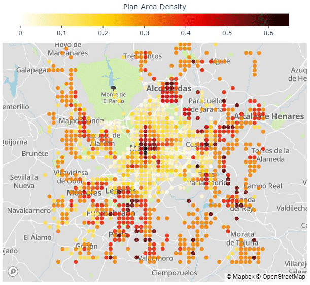
Figure 4Map of the plan area building density over the Madrid region. The map is oriented so that left is west and up is north; the size is 50×50 km. The underlying map was created with © OpenStreetMap contributors 2023. Distributed under the Open Data Commons Open Database License (ODbL) v1.0.
3.1 Subgrid-scale variability in MRT and thermal comfort
In order to understand how urban morphology affects the simulated heat stress, we focus on two grid points with very different urban morphology. One is located in the dense core of the city, with a building plan area density of λP=0.69, and a height-to-width ratio () of 1.6. The second is located in the southern part of the urban area, in a residential neighborhood with a much lower building density (λP=0.2) and a of 0.1.
In Fig. 5, the diurnal evolution of the mean radiant temperature in the six points (three per street direction) is presented for the high-urban-density point and the low-urban-density point. During the daytime, the impact of the shadowing is clear, with reduced mean radiant temperature in the high-density point compared to the more exposed low-density point. On the other hand, during nighttime, the reduced sky-view factor in the high-density point slows down the cooling compared to the more open low-density location.
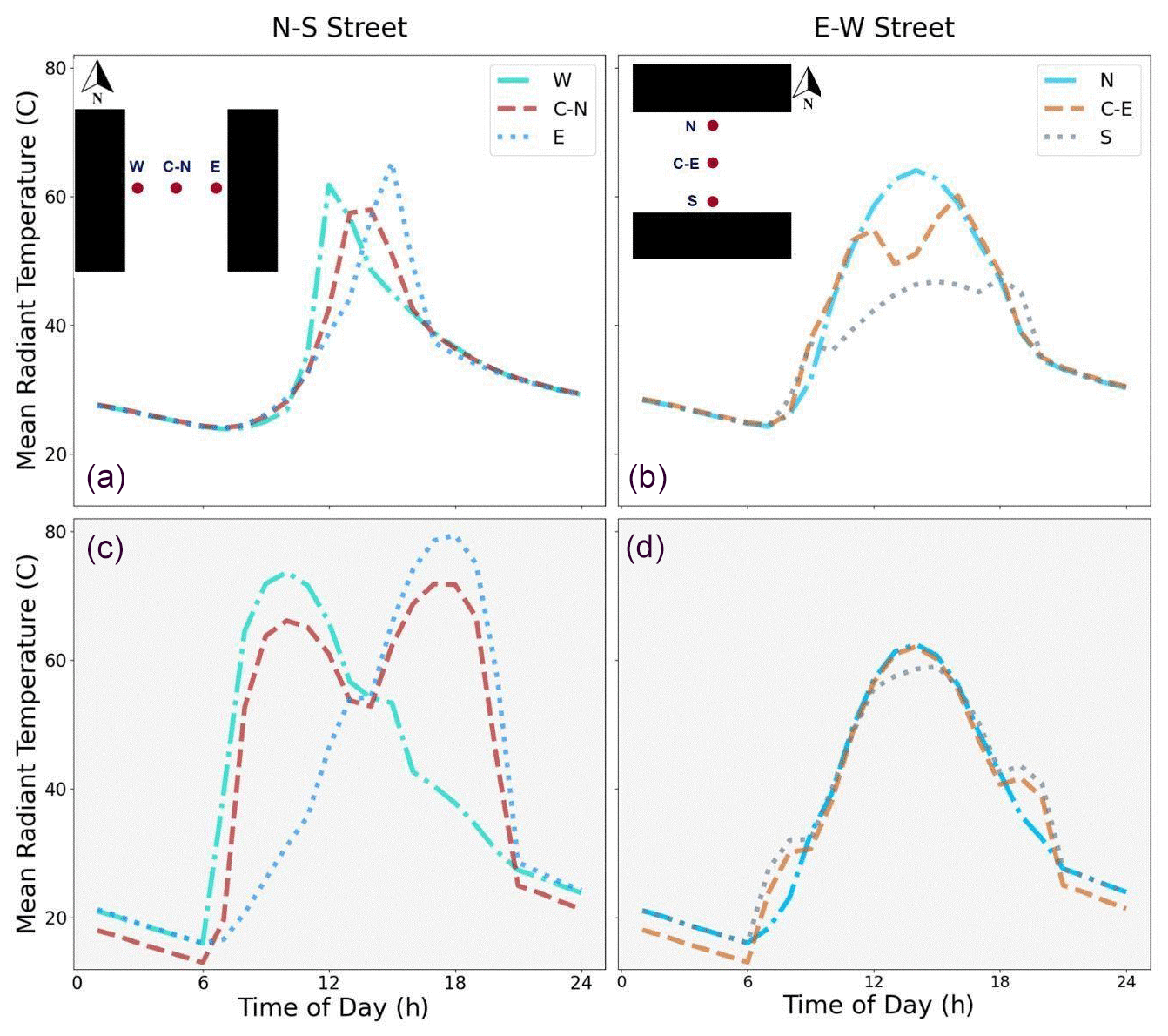
Figure 5Diurnal evolution of MRT for 6 points in the urban canopy. Panels (a) and (b) (white background) correspond to a grid point with the highest building density in the center of Madrid (λP=0.69), while panels (c) and (d) (with a grey background) show MRT in a low-density neighborhood (λP=0.19). The left column is for a N–S street, while the right column shows an E–W street.
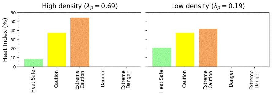
This behavior helps to explain the heat stress index (Fig. 6), which is introduced here as an example of an index that can be computed with standard outputs from meteorological models, i.e., without information related to the radiation environment (e.g., MRT) and urban morphology. The air temperature indicates hotter values during both the day and the night in the high-urban-density point compared to the low-density location. The heat index, which considers air temperature and humidity only and does not include mean radiant temperature or wind, shows the same tendency. On the other hand, the UTCI behavior communicates a different and more complete result. In the low-density neighborhood, more exposed to the sun, the UTCI shows a stronger subgrid spatial variability, in particular during the morning and afternoon, with the potential for stronger heat stress than in the high-density neighborhood. During nighttime, the spatial variability is reduced due to reduced MRT variation as the shadowing effect disappears, and higher UTCI values are found at the high-urban-density location. This difference in behavior between the two locations can also be seen in Fig. 7, where the fractions of the 10th percentile of UTCI values (i.e., representative of one of the coolest spots in the grid cell) and the 90th percentile (i.e., one of the hottest) in the different heat stress regimes are shown for the two points. Here we can see that in the low-density urban point, the cool location is in a comfortable UTCI range most of the time, while the hot (90th percentile UTCI) sub grid location is under stress most of the time. On the other hand, less variability is present in the high-density neighborhood, with fewer extreme values, and most of the time it is in the strong or moderate heat stress regime for both the cool and hot locations within the grid square. This kind of detail is not available from the heat index distribution which does not account for the mean radiant temperature, wind, or their variabilities (Fig. 8).
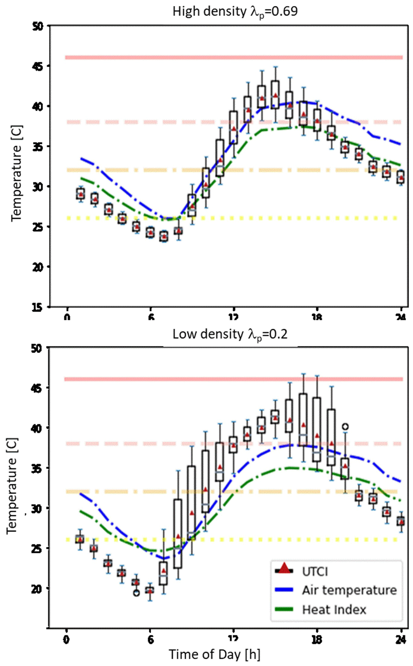
Figure 6Diurnal evolution of UTCI compared with 2 m air temperature and heat index calculated from air temperature and relative humidity at each grid point). The UTCI boxplot at each hour represents the subgrid-scale distribution calculated based on six MRT, three wind speed, and three air temperature values (54 combinations in total). The horizontal lines represent the thermal comfort zones for UTCI (i.e., above +46 °C: extreme heat stress; +38 to +46 °C: very strong heat stress; +32 to +38 °C: strong heat stress; +26 to +32 °C: moderate heat stress; and +9 to +26 °C: no thermal stress).

Figure 7From top to bottom, the frequency of UTCI class over a 24 h period, for a subgrid location that is cooler (i.e., 10th percentile of UTCI in the urban canopy; a, b) and for a subgrid location that is hotter (i.e., 90th percentile of UTCI in the urban canopy; c, d) for the high-density (a, c) and low-density (b, d) points.
3.2 City-scale maps of outdoor thermal comfort and heat stress indicators
The previous analysis helps to understand the spatial distribution of the different variables presented in Figs. 9 at 10 at 16:00 UTC (note that Madrid is at a longitude of 3° W, so UTC is essentially equal to solar time). In the dense city center, the distribution of 2 m air temperature at 09:00 UTC shows a hot region, with cooler areas in the less dense regions around it. This effect is due to the fact that in the dense region, the reduced sky-view factor of the streets (high ) as well as the larger thermal storage capacity in the buildings reduce the nocturnal cooling and increase the vertical mixing in that part of the city compared to the surroundings. Such a difference is still visible in the morning. The higher temperatures in the SE part of the urban area and cool temperatures in the NW are the result of the topographical differences. The spatial distribution of air temperature is qualitatively similar to the spatial distribution of the 10th percentile of UTCI (e.g., the cool spot in the grid cell) even if the differences between the center and the surrounding urban areas are not as intense as for 2 m air temperature. On the other hand, the 90th-percentile map (hot spot) shows a completely different pattern; in the city center, at that time of the day, the whole street is still in the shadow, while in the surrounding, less dense urban areas there are points completely exposed to the sun. As a comparison, the map of surface temperature (a variable often used to represent the spatial distribution of heat in cities) as seen from a satellite, i.e., based only on a weighted average of roof, street, and vegetation temperatures (see full equations in Martilli et al., 2021), does not show a clear pattern, and it is uncorrelated with the other maps. This is a clear indication that this variable should not be used for the assessment of the heat hazard or heat stress in urban areas.
At 16:00 UTC, the air temperature again shows higher values in the city center, lower values in the urban surroundings, and a gradient from hotter SE values at lower elevations to cooler NW at higher elevations (Fig. 10). Such a tendency is present also for the 10th percentile (cool spot) but with less variability. The 90th percentile map (hot spot) indicates that the area with elevated heat stress extends well beyond the city center, including lower-density regions that, even if they have lower air temperatures, are fully exposed to the sun. Finally, as it was the case for 09:00 UTC, the surface temperatures have a map uncorrelated with neither the air temperatures nor the UTCI maps.
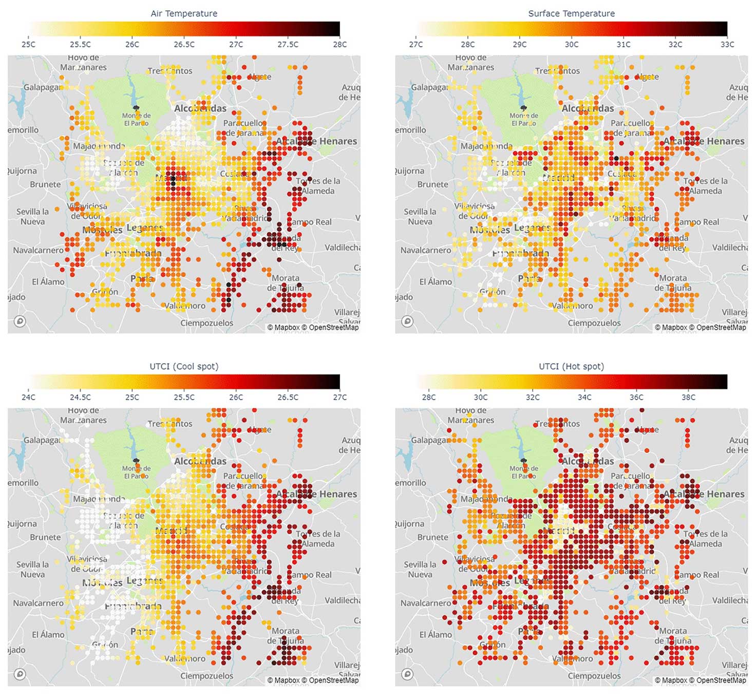
Figure 9Spatial maps at 09:00 UTC for 2 m air temperature (top-left); surface temperature (top-right); UTCI cool spot, e.g., the 10 percentile of UTCI captured in the urban canopy model (bottom-left); and UTCI hot spot, e.g., 90 percentile of UTCI in the urban canopy (bottom-right). Surface temperature is equivalent to that seen by a nadir-view satellite sensor (i.e., an area-weighted average of the canopy ground temperature, roof temperature, and vegetation temperature in non-urban fractions is considered). The underlying maps were created with © OpenStreetMap contributors 2023. Distributed under the Open Data Commons Open Database License (ODbL) v1.0.
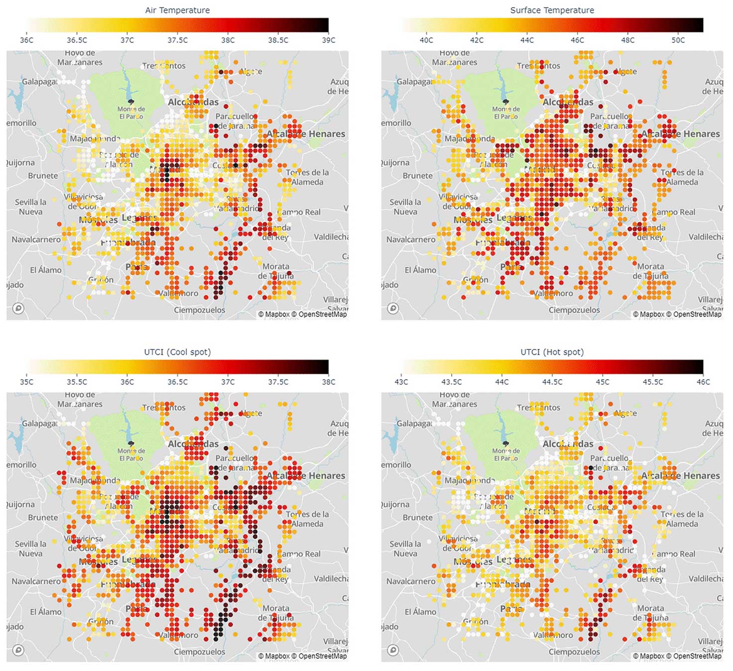
Figure 10Same as Fig. 9 but at 16:00 UTC. The underlying maps were created with © OpenStreetMap contributors 2023. Distributed under the Open Data Commons Open Database License (ODbL) v1.0.
The main limitation of the approach we propose here to account for the subgrid variability in mean radiant temperature is the idealization of the urban morphology adopted by the urban canopy parameterization BEP-BEM. This consists of representing the urban morphology as a series of infinite urban canyons, all with the same width, separated by buildings of constant width and variable building height. Two street orientations are considered for each grid cell: north–south and east–west. The dimensions of the buildings and street canyons are determined so that the building plan area density, the density of urban vertical surfaces per horizontal area, and the mean building heights are equal to those of the real morphology of the grid cell. As a result, the total surface areas of walls, roads, and roofs in the idealized morphology used by BEP-BEM closely approximate the corresponding surface areas in the real neighborhood, and – to a certain extent – the street and buildings of the idealized morphology can be considered representatives of an average street and set of buildings present in the grid cell. The advantage of this approach, common among the most widely used urban canopy parameterizations (Masson, 2000; Kusaka et al., 2001), is that it allows for accurate estimation of shadowing and radiation trapping effects in the urban canopy with low computational cost, without considering the real urban morphology. Keeping the computational cost low was an essential requirement considering the computational resources that were available when these urban canopy parameterizations were developed (about 20 years ago). With today's computational resources, there may be potential for accounting for more complexity in the urban morphology. However, this would require deep changes in the structure of the urban canopy parameterization BEP-BEM that are beyond the scope of the present article. For this reason, we decided to keep the idealized morphology of BEP-BEM and estimate the mean radiant temperature in six locations representative of the middle of the street and the sidewalks. So, the mean radiant temperatures computed are representatives of those six points of an “average” street in the grid cell. Indeed, in a grid cell of a mesoscale model (that typically has a size on the order of 1 km2) there is a variety of street and building dimensions and orientations, so the present approach cannot capture the full spatial variability in mean radiant temperature, a variability that increases with the heterogeneity of the real urban morphology. Nevertheless, it represents a step forward since it accounts for the range (and to some extent, the variability) of mean radiant temperature within the average idealized street canyon that can be reasonably considered the most likely street typology within the grid cell, something that previous approaches do not do. Overall, the current approach is likely to accurately quantify the mean radiant temperature of at least one average shaded pedestrian and one average sunlit pedestrian (during periods with direct shortwave irradiance) and thus capture the largest source of spatial variation in both MRT and UTCI (Middel and Krayenhoff, 2019). Another limitation of the approach presented here is the lack of street trees. Currently, work is in progress to introduce trees in the version of BEP-BEM implemented in WRF via implementation of the BEP-Tree model (Krayenhoff et al., 2020) and in this way account for their impacts on mean radiant temperature as well as on air temperature, humidity, and wind.
The approach used to estimate the mean wind speed and its subgrid variability is grounded on a large number of CFD simulations over a variety of urban morphologies. Indeed, as shown in Fig. 3, the subgrid variability in wind speed can be quite large and certainly strongly influenced by the relative arrangements of buildings and streets. So, the approach presented here likely underestimates the subgrid variability in wind speed – and this is why we decided to give the same likelihood to the three values of wind speed estimated in Eq. (6) instead of assuming a Gaussian or Weibull distribution of the probabilities of wind speed in the grid cell. To fully capture this variability, a complete coupling between the mesoscale model and a detailed CFD model would be needed – something that we may be able to do in the near future but is still unavailable with the current computational resources. Another limitation of the present approach is that the CFD simulations used to build the database from which the parameterization has been derived are all for a neutral atmosphere, so thermal effects on wind speed and its subgrid variability are neglected.
A new parameterization to quantify intra-neighborhood heat stress variability in urban areas using a mesoscale model is presented. This approach is based on two primary developments: (1) calculation of mean radiant temperature at several locations within the idealized urban morphology used by the urban canopy model BEP-BEM and (2) parameterization of mean wind speed and its subgrid spatial variability as a function of the local urban morphology and the mean wind velocity computed by the WRF mesoscale model using relations developed from a large suite of CFD simulations over a range of realistic and idealized urban neighborhoods. The components of the new parameterization have been validated against microscale model results. From this approach, the subgrid variability in a heat stress index (i.e., UTCI or SET) can be computed for every grid point, permitting quantification of the heat exposure at both cool and hot locations within each grid square at each time. The new parameterization has been implemented in the multilayer scheme BEP-BEM in WRF and used to simulate a heat wave day over Madrid (Spain) as proof of concept. The results of this initial application demonstrate the following:
- i.
The new parameterization gives information that is more suitable for the evaluation of heat stress than the air temperature due to it being based on an index (UTCI or SET) that also combines air humidity, wind speed, and mean radiant temperature.
- ii.
The new parameterization provides substantively more information than air temperature alone (or any other index that does not account for the mean radiant temperature). It provides information about the subgrid variability (such that heat stress in both cool and hot locations in each grid square is quantified). To our knowledge, this has not been done before with a mesoscale model.
- iii.
The results for the investigated case indicate a strong intra-urban variability, both in air temperature and UTCI values, that can be linked to the differences in urban morphology and elevation above sea level. The ability to assess the differential impacts of urban morphology on heat stress is key to the provision of guidance for urban planning strategies that mitigate urban overheating.
- iv.
Nadir-view surface temperature (i.e., as seen from a satellite-mounted remote sensor) is poorly correlated with both air temperature and UTCI maps, indicating that despite its ubiquitous use at present, it is unlikely to be an adequate metric for heat impact assessment studies.
Finally, we consider that this new development introduces a new methodology for deploying mesoscale models to assess urban overheating mitigation strategies.
As explained in the text, the mean radiant temperature on the pedestrian level is represented using Eq. (1). The full expression of the longwave radiation components for the vertical faces of the pedestrian (L1,L2) for the case of an urban morphology with buildings of constant height and walls with no windows is as follows:
where (see Fig. A1) ψ1i,p is the view factor from wall section i of building 1 to side 1 of the pedestrian. εW is the emissivity of the wall. is the longwave radiation reaching section i of the wall of building 1. T1i is the surface temperature of section i of the wall of building 1. ψ1G,p is the view factor from the ground (or street) to side 1 of the pedestrian. εG is the emissivity of the ground. R1G is the longwave radiation reaching the ground (street). TG is the surface temperature of the ground (street). ψ1S,p is the view factor from the sky to side 1 of the pedestrian. R1S is the longwave radiation from the sky and σ is the Stefan–Boltzmann constant.
Similar meaning applies for side and building 2.
The values of the surface temperatures and the longwave radiations are computed with BEP-BEM. The view factors are estimated based on Eqs. (A13)–(A19) of Martilli et al. (2002) using a height for the pedestrian of 1.8 m.
For the longwave radiation reaching the top of the pedestrian, we made the simple assumption that it is equal to the radiation coming from the sky, L3=RlS, while for the longwave radiation reaching the bottom of the pedestrian, the assumption is that it is equal to the radiation emitted and reflected by the ground or . We consider that these assumptions are reasonable, giving that the contribution of the radiation reaching the top and bottom of the pedestrian is only 6 % each to the final value of the mean radiant temperature. A similar approach is followed for the shortwave radiation, leading to
where is the shortwave radiation reaching section i of the wall of building 1. αi albedo of section i of the wall of the building. RsG is the shortwave radiation reaching the ground. αG is the albedo of the ground. Rs1S is the shortwave radiation from the sun directly reaching side 1 of the pedestrian, computed using Eq. (A10) of Martilli et al. (2002), with the height of the pedestrian of 1.8 m.
The meaning is similar for side and wall 2.
Regarding the radiation reaching the top of the pedestrian, K3, for simplicity only, the radiation coming directly from the sun is considered without accounting for the reflection from the walls. So, the value is zero if the pedestrian is in full shadow, and to estimate it, the formula used is from Eq. (A11) of Martilli et al. (2002). The value of the radiation reaching the bottom of the pedestrian is the value reflected by the ground or K3=αGRsG,
Shortwave radiation is an essential component of the MRT. Below we compare the shortwave radiation reaching the vertical sides of the segment representing the human body computed by BEP-BEM with those estimated with the more detailed model, TUF-Pedestrian.
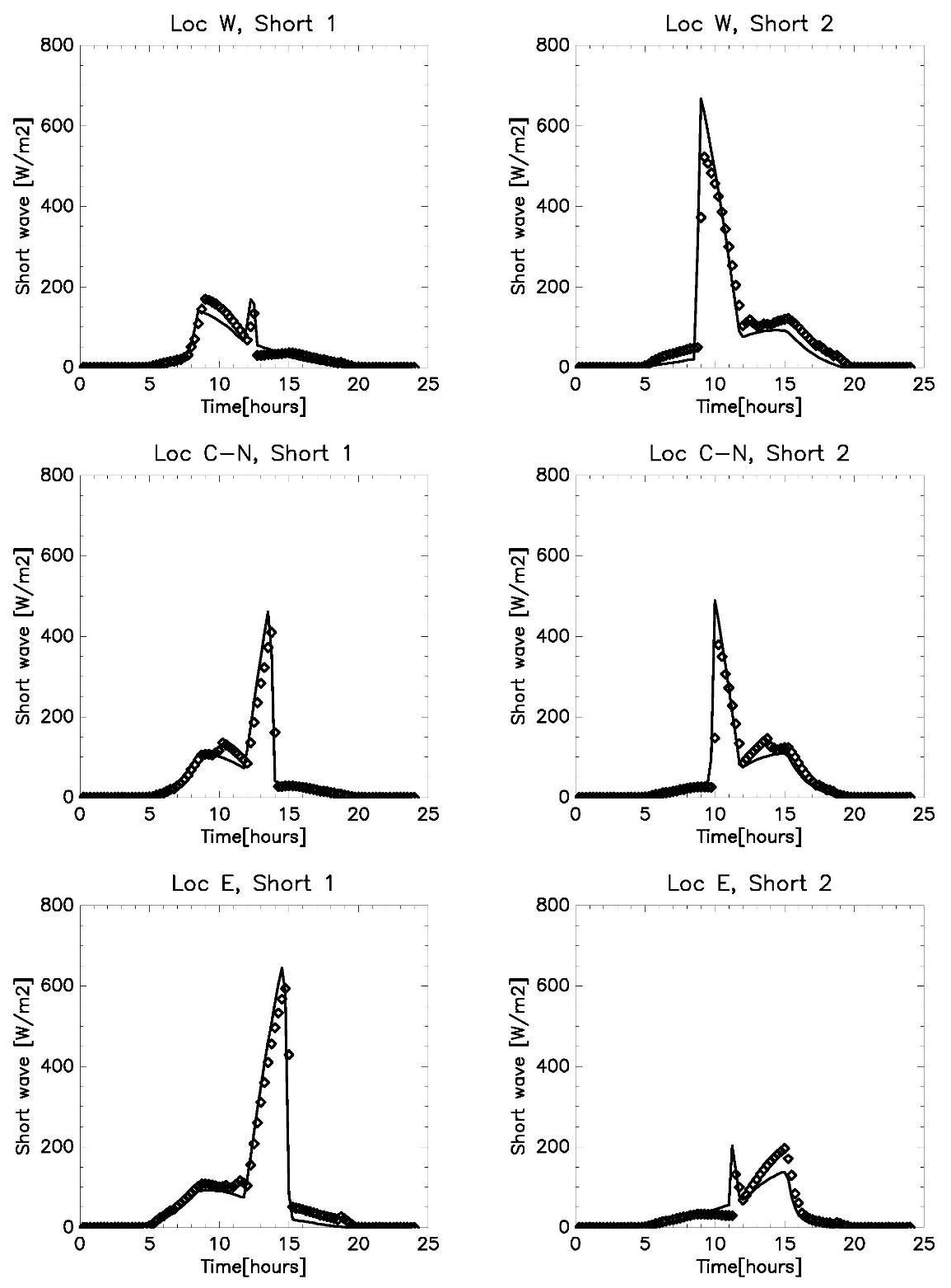
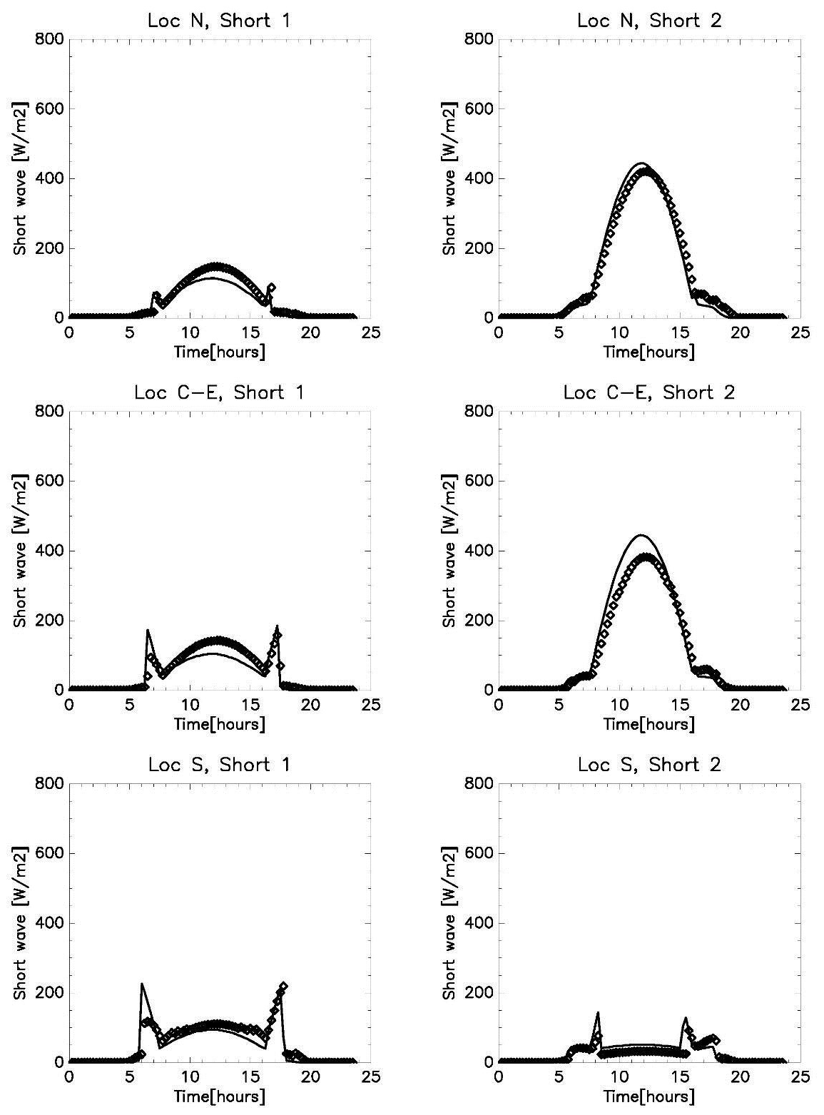
Figure B1Comparison between shortwave radiation at the two sides of the vertical segment representing the pedestrian for the N–S-oriented street. Solid line is the WRF, while diamonds are TUF. Short 1 denotes side 1 of the pedestrian, while Short 2 denotes side 2.
Data from over 173 microscale CFD simulations of urban airflow are considered over-realistic and idealized urban configurations, spanning a wide range of building plan area (λP), frontal area (λF), and wall area (λw) densities representative of realistic urban neighborhoods in different types of cities. CFD simulations are conducted using large-eddy simulations (LES; 162 cases) and Reynolds-averaged Navier–Stokes (RANS; 11 cases) schemes detailed in Table C1.
Table C1Details of CFD microscale simulation cases considered in this study. Simulations are classified based on the configuration (urban form) used. These classifications include UA (uniform height with aligned configuration), US (uniform height with staggered configuration), VA (variable height with aligned configuration), VS (variable height with staggered configuration), UR (uniform height with realistic configuration), and VR-WD (variable height with realistic configuration and multiple wind directions considered).
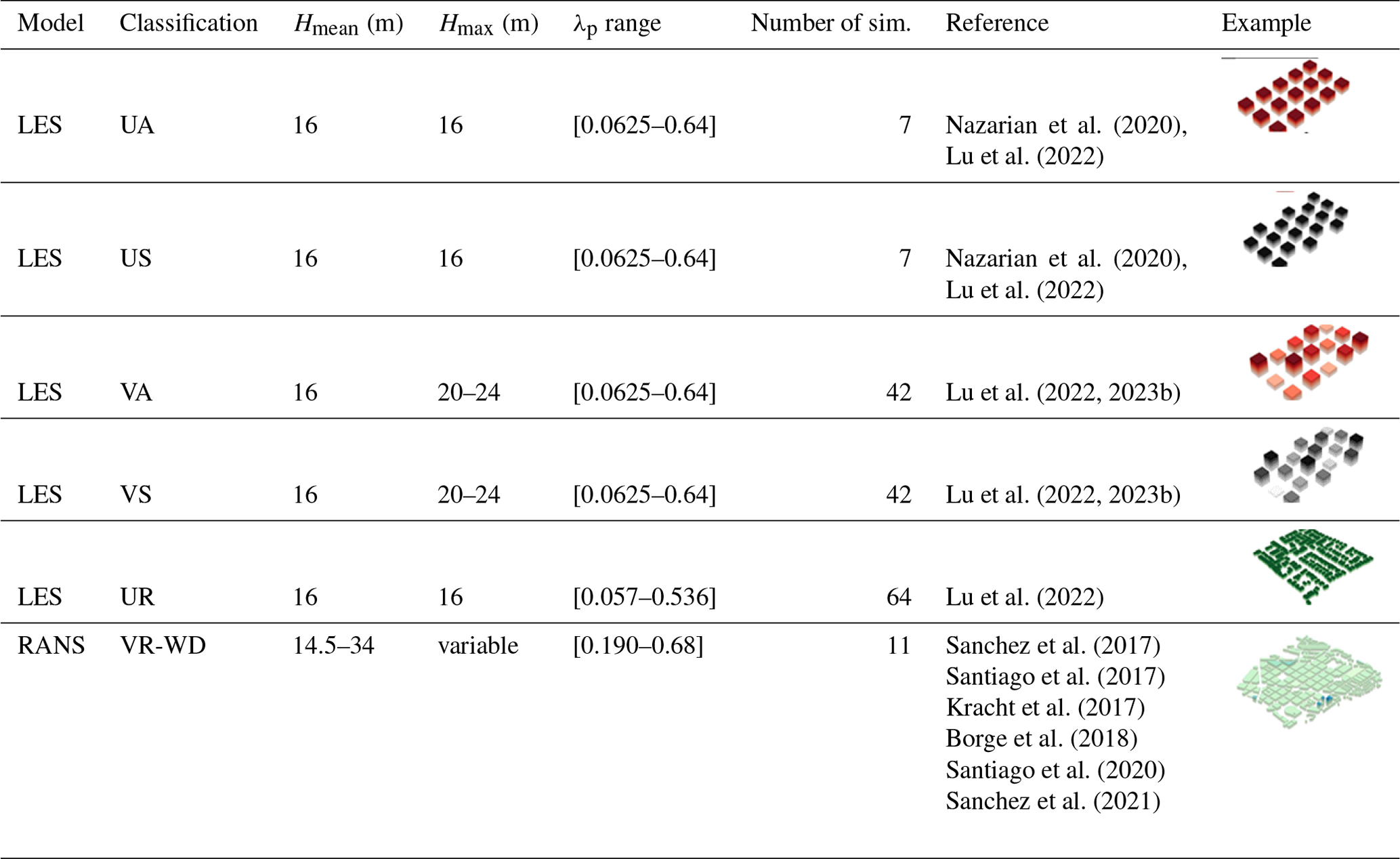
In the LES simulations, airflow over idealized and realistic urban arrays is used to determine the model parameters (Nazarian et al., 2020; Lu et al., 2023a, b). Realistic urban layouts are prepared by rasterizing building footprints from an open-source dataset, OpenStreetMap, using OSM2LES (Lu et al., 2022). Assuming uniform building height (Table C1), 64 realistic urban neighborhoods were obtained from several major cities such as Sydney and Melbourne (Australia); Barcelona (Spain); and Detroit, Los Angeles, and Chicago (United States). Idealized urban arrays are considered in an aligned and staggered arrangement that follows (Coceal et al., 2007), with varying urban density (λp in [0.0625,0.64]) and height variability (Hstd= [0 m, 2.8 m, 5.6 m]). Simulations are conducted in the Parallelized Large-Eddy Simulation Model (PALM version r4554) (Maronga et al., 2020) following the same setup in Nazarian et al. (2020), which validated results against direct numerical simulation (Coceal et al., 2007) and wind tunnel experiments (Brown et al., 2001). The computational domain is discretized using the second-order central differences (Piacsek and Williams, 1970), where the horizontal grid spacing is uniform and the vertical spacing follows the staggered Arakawa C-grid. The minimal storage scheme is employed in the time integration to solve the filtered prognostic incompressible Boussinesq equations, where the pressure perturbation was calculated using Poisson's equation and was solved by the FFTW scheme (Frigo and Johnson, 1998). FFTW is a C subroutine library for computing the discrete Fourier transform (DFT) in one or more dimensions.
The RANS dataset is derived from steady-state CFD-RANS simulations performed with the realizable k-ε turbulence model (STAR-CCM+; Siemens, 2023) over realistic urban areas. The size of the computational domains is determined following the best practice guideline of COST Action 732 (Franke et al., 2010). The horizontal area covers around 1–1.5 km2 and the domain top is at around 8H, H being the mean height of buildings. The resolution of the irregular polyhedral mesh used in all CFD-RANS simulations goes from 0.5 m close to buildings to 6 m out of the built-up area, which results in between 3 and 8 million grid points depending on the complexity of the geometry. Inlet vertical profiles for wind speed, turbulent kinetic energy (k), and its dissipation (ε) are established in neutral atmospheric conditions. The evaluation of the CFD-RANS simulations was addressed in previous studies, with more information provided in previous publications.
The code of WRF-Comfort can be obtained at https://doi.org/10.5281/zenodo.7951433 (Martilli, 2023a).
The results of the simulation over Madrid shown in the paper are stored at https://doi.org/10.5281/zenodo.8199017 (Martilli, 2023b).
AM, NN, and ESK designed the methodology; AM developed the model code; AM and ARS performed the mesoscale simulations; JaL and ESK performed the TUF-3D simulations; JiL, ER, BS, and JLS performed the microscale LES and RANS simulations; NN prepared the figures; and AM, NN, and ESK prepared the paper with contributions from all co-authors.
The contact author has declared that none of the authors has any competing interests.
Publisher’s note: Copernicus Publications remains neutral with regard to jurisdictional claims made in the text, published maps, institutional affiliations, or any other geographical representation in this paper. While Copernicus Publications makes every effort to include appropriate place names, the final responsibility lies with the authors.
Alberto Martilli's contribution has been supported by the CROCUS project funded by DOE BER (grant no. DE-FOA-0002581).
This paper was edited by Jinkyu Hong and reviewed by three anonymous referees.
Borge, R., Santiago, J. L., de la Paz, D., Martín, F., Domingo, J., Valdés, C., Sánchez B., Rivas, E., Rozas, M. T., Lázaro, S., Pérez, J., and Fernández, A.: Application of a short term air quality action plan in Madrid (Spain) under a high-pollution episode-Part II: Assessment from multi-scale modelling, Sci. Total Environ., 635, 1574–1584, https://doi.org/10.1016/j.scitotenv.2018.04.323, 2018.
Bougeault, P. and Lacarrere, P.: Parameterization of Orography-Induced Turbulence in a Mesobeta–Scale Model, Mon. Weather Rev., 117, 1872–1890, https://doi.org/10.1175/1520-0493(1989)117<1872:POOITI>2.0.CO;2, 1989.
Broadbent, A. M., Krayenhoff, E. S., and Georgescu, M.: The motley drivers of heat and cold exposure in 21st century US cities, P. Natl. Acad. Sci. USA, 117, 21108–21117, https://doi.org/10.1073/pnas.2005492117, 2020.
Brousse, O., Martilli, A., Foley, M., Mills, G., and Bechtel, B.: WUDAPT, an efficient land use producing data tool for mesoscale models? Integration of urban LCZ in WRF over Madrid, Urban Clim., 17, 116–134, https://doi.org/10.1016/j.uclim.2016.04.001, 2016.
Brown, M. J., Lawson, R. E., DeCroix, D. S., and Lee, R. L.: Comparison of centerline velocity measurements obtained around 2D and 3D building arrays in a wind tunnel, Int. 40 Soc. Environ. Hydraulics, Tempe, AZ, 5, 495, OSTI ID: 783425, https://digital.library.unt.edu/ark:/67531/metadc716934/m2/1/high_res_d/783425.pdf (last access: 25 June 2024), 2001
Coceal, O., Dobre, A., Thomas, T. G., and Belcher, S. E.: Structure of turbulent flow over regular arrays of cubical roughness, J. Fluid Mech., 589, 375–409, https://doi.org/10.1017/S002211200700794X, 2007.
Franke, J., Hellsten, A., Schlünzen, H., and Carissimo, B.: The Best Practise Guideline for the CFD simulation of flows in the urban environment: an outcome of COST 732, in: The Fifth International Symposium on Computational Wind Engineering (CWE2010), 1–10, ISBN 3-00-018312-4, 2010.
Frigo, M. and Johnson, S. G.: FFTW: an adaptive software architecture for the FFT, in: Proceedings of the 1998 IEEE International Conference on Acoustics, Speech and Signal Processing, ICASSP '98 (Cat. No.98CH36181), vol. 3, 1381–1384, https://doi.org/10.1109/ICASSP.1998.681704, 1998.
Gagge, A. P., Fobelets, A. P., and Berglund, L.: A standard predictive index of human response to the thermal environment, ASHRAE T., 92, 709–731, 1986.
Geletič, J., Lehnert, M., Savić, S., and Milošević, D.: Modelled spatiotemporal variability of outdoor thermal comfort in local climate zones of the city of Brno, Czech Republic, Sci. Total Environ., 624, 385–395, https://doi.org/10.1016/j.scitotenv.2017.12.076, 2018.
Giannaros, T. M., Lagouvardos, K., Kotroni, V., and Matzarakis, A.: Operational forecasting of human-biometeorological conditions, Int. J. Biometeorol., 62, 1339–1343, 2018.
Giannaros, C., Agathangelidis, I., Papavasileiou, G., Galanaki, E., Kotroni, V., Lagouvardos, K., and Matzarakis, A.: The extreme heat wave of July–August 2021 in the Athens urban area (Greece): Atmospheric and human-biometeorological analysis exploiting ultra-high resolution numerical modeling and the local climate zone framework, Sci. Total Environ., 857, 159300, https://doi.org/10.1016/j.scitotenv.2022.159300, 2023.
Höppe, P.: The physiological equivalent temperature – a universal index for the biometeorological assessment of the thermal environment, Int. J. Biometeorol., 43, 71–75, https://doi.org/10.1007/s004840050118, 1999.
Jendritzky, G., de Dear, R., and Havenith, G.: UTCI – Why another thermal index?, Int. J. Biometeorol., 56, 421–428, https://doi.org/10.1007/s00484-011-0513-7, 2012.
Jiang, T., Krayenhoff, E. S., Voogt, J. A., Warland, J., Demuzere, M., and Moede, C.: Dynamically downscaled projection of urban outdoor thermal stress and indoor space cooling during future extreme heat, Urban Clim., 51, 101648, https://doi.org/10.1016/j.uclim.2023.101648, 2023.
Jin, L., Schubert, S., Fenner, D., Salim, M. H., and Schneider, C.: Estimation of mean radiant temperature in cities using an urban parameterization and building energy model within a mesoscale atmospheric model, Meteorol. Z., 31, 31–52, 2022.
Kracht, O., Santiago, J., Martin, F., Piersanti, A., Cremona, G., Righini, G., Vitali, L., Delaney, K., Basu, B., Ghosh, B., Spangl, W., Brendle, C., Latikka, J., Kousa, A., Pärjälä, E., Meretoja, M., Malherbe, L., Letinois, L., Beauchamp, M., Lenartz, F., Hutsemekers, V., Nguyen, L., Hoogerbrugge, R., Eneroth, K., Silvergren, S., Hooyberghs, H., Viaene, P., Maiheu, B., Janssen, S., Roet, D., and Gerboles, M., Spatial representativeness of air quality monitoring sites: Outcomes of the FAIRMODE/AQUILA intercomparison exercise, EUR 28987 EN, Publications Office of the European Union, Luxembourg, ISBN 978-92-79-77218-4, JRC108791, https://doi.org/10.2760/60611, 2017.
Krayenhoff, E. S., Moustaoui, M., Broadbent, A. M., Gupta, V., and Georgescu, M.: Diurnal interaction between urban expansion, climate change and adaptation in US cities, Nat. Clim. Change, 8, 1097–1103, https://doi.org/10.1038/s41558-018-0320-9, 2018.
Krayenhoff, E. S., Jiang, T., Christen, A., Martilli, A., Oke, T. R., Bailey, B. N., and Crawford, B. R.: A multi-layer urban canopy meteorological model with trees (BEP-Tree): Street tree impacts on pedestrian-level climate, Urban Clim., 32, 100590, https://doi.org/10.1016/j.uclim.2020.100590, 2020.
Kusaka, H., Kondo, H., Kikegawa, Y., and Kimura, F.: A simple single-layer urban canopy model for atmospheric models: Comparison with multi-layer and slab models, Bound.-Lay. Meteorol., 101, 329–358, 2001.
Lachapelle, J. A., Krayenhoff, E. S., Middel, A., Meltzer, S., Broadbent, A. M., and Georgescu, M.: A microscale three-dimensional model of urban outdoor thermal exposure (TUF-Pedestrian), Int. J. Biometeorol., 66, 833–848, https://doi.org/10.1007/s00484-022-02241-1, 2022.
Lemonsu, A., Viguié, V., Daniel, M., and Masson, V.: Vulnerability to heat waves: Impact of urban expansion scenarios on urban heat island and heat stress in Paris (France), Urban Clim., 14, 586–605, https://doi.org/10.1016/j.uclim.2015.10.007, 2015.
Leroyer, S., Bélair, S., Spacek, L., and Gultepe, I.: Modelling of radiation-based thermal stress indicators for urban numerical weather prediction, Urban Clim., 25, 64–81, https://doi.org/10.1016/j.uclim.2018.05.003, 2018.
Lu, J., Nazarian, N., and Hart, M.: OSM2LES – A Python-based tool to prepare realistic urban geometry for LES simulation from OpenStreetMap (0.1.0), Zenodo [code], https://doi.org/10.5281/zenodo.6566346, 2022.
Lu, J., Nazarian, N., Hart, M., Krayenhoff, S., and Martilli, A.: Novel geometric parameters for assessing flow over realistic versus idealized urban arrays, J. Adv. Model. Earth Sy., 15, e2022MS003287, https://doi.org/10.1029/2022MS003287, 2023a.
Lu, J., Nazarian, N., Hart, M., Krayenhoff, S., and Martilli, A.: Representing the effects of building height variability on urban canopy flow, Q. J. Roy. Meteor. Soc., 150, 46–67, https://doi.org/10.1002/qj.4584, 2023b.
Maronga, B., Banzhaf, S., Burmeister, C., Esch, T., Forkel, R., Fröhlich, D., Fuka, V., Gehrke, K. F., Geletič, J., Giersch, S., Gronemeier, T., Groß, G., Heldens, W., Hellsten, A., Hoffmann, F., Inagaki, A., Kadasch, E., Kanani-Sühring, F., Ketelsen, K., Khan, B. A., Knigge, C., Knoop, H., Krč, P., Kurppa, M., Maamari, H., Matzarakis, A., Mauder, M., Pallasch, M., Pavlik, D., Pfafferott, J., Resler, J., Rissmann, S., Russo, E., Salim, M., Schrempf, M., Schwenkel, J., Seckmeyer, G., Schubert, S., Sühring, M., von Tils, R., Vollmer, L., Ward, S., Witha, B., Wurps, H., Zeidler, J., and Raasch, S.: Overview of the PALM model system 6.0, Geosci. Model Dev., 13, 1335–1372, https://doi.org/10.5194/gmd-13-1335-2020, 2020.
Martilli, A.: WRF-comfort, Zenodo [code], https://doi.org/10.5281/zenodo.7951433, 2023a.
Martilli, A.: data shown in manuscript “WRF-Comfort: Simulating micro-scale variability of outdoor heat stress at the city scale with a mesoscale model”, Zenodo [data set], https://doi.org/10.5281/zenodo.8199017, 2023b.
Martilli, A., Clappier, A., and Rotach, M. W.: An Urban Surface Exchange Parameterisation for Mesoscale Models, Bound.-Lay. Meteorol., 104, 261–304, https://doi.org/10.1023/A:1016099921195, 2002.
Martilli, A., Sanchez, B., Rasilla, D., Pappaccogli, G., Allende, F., Martin, F., Róman-Cascón, C., Yagüe, C., and Fernandez, F: Simulating the meteorology during persistent Wintertime Thermal Inversions over urban areas, The case of Madrid, Atmos. Res., 263, 105789, https://doi.org/10.1016/j.atmosres.2021.105789, 2021.
Martilli, A., Sánchez, B., Santiago, J. L., Rasilla, D., Pappaccogli, G., Allende, F., Martín, F., Roman-Cascón, C., Yagüe, C., and Fernández, F.: Simulating the pollutant dispersion during persistent Wintertime thermal Inversions over urban areas. The case of Madrid, Atmos. Res., 270, 106058, https://doi.org/10.1016/j.atmosres.2022.106058, 2022.
Masson, V.: A physically-based scheme for the urban energy budget in atmospheric models, Bound.-Lay. Meteorol., 94, 357–397, 2000.
Matzarakis, A., Rutz, F., and Mayer, H.: Modelling radiation fluxes in simple and complex environments – application of the RayMan model, Int. J. Biometeorol., 51, 323–334, https://doi.org/10.1007/s00484-006-0061-8, 2007.
Middel, A. and Krayenhoff, E. S.: Micrometeorological determinants of pedestrian thermal exposure during record-breaking heat in Tempe, Arizona: Introducing the MaRTy observational platform, Sci. Total Environ., 687, 137–151, 2019.
Nazarian, N., Fan, J., Sin, T., Norford, L., and Kleissl, J.: Predicting outdoor thermal comfort in urban environments: A 3D numerical model for standard effective temperature, Urban Clim., 20, 251–267, https://doi.org/10.1016/j.uclim.2017.04.011, 2017.
Nazarian, N., Martilli, A., and Kleissl, J.: Impacts of realistic urban heating, part I: spatial variability of mean flow, turbulent exchange and pollutant dispersion, Bound.-Lay. Meteorol., 166, 367–393, 2018.
Nazarian, N., Acero, J. A., and Norford, L.: Outdoor thermal comfort autonomy: Performance metrics for climate-conscious urban design, Build. Environ., 155, 145–160, https://doi.org/10.1016/j.buildenv.2019.03.028, 2019.
Nazarian, N., Krayenhoff, E. S., and Martilli, A.: A one-dimensional model of turbulent flow through “urban” canopies (MLUCM v2.0): updates based on large-eddy simulation, Geosci. Model Dev., 13, 937–953, https://doi.org/10.5194/gmd-13-937-2020, 2020.
Nazarian, N., Krayenhoff, E. S., Bechtel, B., Hondula, D. M., Paolini, R., Vanos, J., Cheung, T., Chow, W. T. L., de Dear, R., Jay, O., Lee, J. K. W., Martilli, A., Middel, A., Norford, L. K., Sadeghi, M., Schiavon, S., and Santamouris, M.: Integrated assessment of urban overheating impacts on human life, Earths Future, 10, e2022EF002682, https://doi.org/10.1029/2022ef002682, 2022.
Piacsek, S. A. and Williams, G. P.: Conservation properties of convection difference schemes, J. Comput. Phys., 6, 392–405, https://doi.org/10.1016/0021-9991(70)90038-0, 1970.
Pigliautile, I., Pisello, A. L., and Bou-Zeid, E.: Humans in the city: Representing outdoor thermal comfort in urban canopy models, Renew. Sustain Energ. Rev., 133, 110103, https://doi.org/10.1016/j.rser.2020.110103, 2020.
Potchter, O., Cohen, P., Lin, T. P., and Matzarakis, A.: Outdoor human thermal perception in various climates: A comprehensive review of approaches, methods and quantification, Sci. Total. Environ., 1, 390–406, https://doi.org/10.1016/j.scitotenv.2018.02.276, 2018.
Rodriguez-Sanchez, A.: Simulación de olas de calor en la ciudad de Madrid, Master Thesis, Universidad Complutense de Madrid, https://www.researchgate.net/publication/353350538_Simulacion_de_olas_de_calor_en_la_ciudad_de_Madrid#fullTextFileContent (last access: 24June 2024), 2020.
Salamanca, F., Krpo, A., Martilli, A., and Clappier, A.: A new building energy model coupled with an urban canopy parameterization for urban climate simulations—part I. formulation, verification, and sensitivity, Theor. Appl. Climatol., 99, 331–344, https://doi.org/10.1007/s00704-009-0142-9, 2010.
Salamanca, F., Martilli, A., and Yagüe, C.: A numerical study of the Urban Heat Island over Madrid during the DESIREX (2008) campaign with WRF and an evaluation of simple mitigation strategies, Int. J. Climatol., 32, 2372–2386, https://doi.org/10.1002/joc.3398, 2012.
Santiago, J. L., Krayenhoff, E. S., and Martilli, A.: Flow simulations for simplified urban configurations with microscale distributions of surface thermal forcing, Urban Clim., 9, 115–133, https://doi.org/10.1016/j.uclim.2014.07.008, 2014.
Santiago, J. L., Rivas, E., Sanchez, B., Buccolieri, R., and Martin, F.: The impact of planting trees on NOx concentrations: The case of the Plaza de la Cruz neighbourhood in Pamplona (Spain), Atmosphere, 8, p. 131, https://doi.org/10.3390/atmos8070131, 2017.
Santiago, J. L., Sanchez, B., Quaassdorff, C., de la Paz, D., Martilli, A., Martín, F., Borge, R., Rivas, E., Gómez-Moreno, F. J., Díaz, E. and Artiñano, B., Yagüe, C., and Vardoulakis, S.: Performance evaluation of a multiscale modelling system applied to particulate matter dispersion in a real traffic hot spot in Madrid (Spain), Atmos. Pollut. Res., 11, 141–155, https://doi.org/10.1016/j.apr.2019.10.001, 2020.
Sanchez, B., Santiago, J. L., Martilli, A., Palacios, M., Núñez, L., Pujadas, M., and Fernández-Pampillón, J.: NOx depolluting performance of photocatalytic materials in an urban area – Part II: assessment through computational fluid dynamics simulations, Atmos. Environ., 246, 118091, https://doi.org/10.1016/j.atmosenv.2020.118091, 2021.
Sanchez, B., Santiago, J. L., Martilli, A., Martin, F., Borge, R., Quaassdorff, C., and de la Paz, D.: Modelling NOx concentrations through CFD-RANS in an urban hot-spot using high resolution traffic emissions and meteorology from a mesoscale model, Atmos. Environ., 163, 155–165, https://doi.org/10.1016/j.atmosenv.2017.05.022, 2017.
Siemens Digital Industries, Simcenter STAR-CCM+ software, Software, https://plm.sw.siemens.com/en-US/simcenter/fluids-thermal-simulation/star-ccm/ (last access: 25 June 2024), 2023.
Skamarock, W. C., Klemp, J. B., Dudhia, J., Gill, D. O., Liu, Z., Berner, J., Wang, W., Powers, J. G., Duda, M. G., Barker, D. M., and Huag, X.-Y.: A description of the advanced research WRF model version 4, National Center for Atmospheric Research, Boulder, CO, USA, 145, 550, https://doi.org/10.5065/1dfh-6p97, 2019.
Thorsson, S., Lindberg, F., Eliasson, I., and Holmer, B.: Different methods for estimating the mean radiant temperature in an outdoor urban setting, Int. J. Climatol., 27, 1983–1993, 2007.
Tuholske, C., Caylor, K., Funk, C., Verdin, A., Sweeney, S., Grace, K., Peterson, P., and Evans, T.: Global urban population exposure to extreme heat, P. Natl. Acad. Sci. USA, 118, e2024792118, https://doi.org/10.1073/pnas.2024792118, 2021.
Zhang, J., Li, Z., and Hu, D.: Effects of urban morphology on thermal comfort at the micro-scale, Sustain. Cities Soc., 86, 104150, https://doi.org/10.1016/j.scs.2022.104150, 2022.
Zhao, L., Oleson, K., Bou-Zeid, E., Krayenhoff, E. S., Bray, A., Zhu, Q., Zheng, Z., Chen, C., and Oppenheimer, M.: Global multi-model projections of local urban climates, Nat. Clim. Chang., 11, 152–157, https://doi.org/10.1038/s41558-020-00958-8, 2021.
- Abstract
- Introduction
- Methodology
- Characterization of thermal comfort in regional-scale models: Madrid case
- Limitations
- Conclusions
- Appendix A: Computation of radiation for mean radiant temperature
- Appendix B: Comparison between shortwave calculations in BEP-BEM and TUF-Pedestrian
- Appendix C: CFD simulations for wind speed variability
- Code and data availability
- Author contributions
- Competing interests
- Disclaimer
- Financial support
- Review statement
- References