Sweep interpolation: a cost-effective semi-Lagrangian scheme in the Global Environmental Multiscale model

The interpolation process is the most computationally expensive step of the semi-Lagrangian (SL) approach for solving advection and is commonly used in numerical weather prediction (NWP) models. It has a significant impact on the accuracy of the solution and can potentially be the most expensive part of model integration. The sweep algorithm, which was first described by Mortezazadeh and Wang (2017), performs SL interpolation with the same computational cost as a third-order polynomial scheme but at the accuracy of the fourth order. This improvement is achieved by using two third-order backward and forward polynomial interpolation schemes in two consecutive time steps. In this paper, we present a new application of the sweep algorithm within the context of global forecasts produced with Environment Climate Change Canada's Global Environmental Multiscale (GEM) model. Results show that the SL scheme with sweep interpolation is computationally more efficient compared to a conventional SL scheme with fourth-order polynomial interpolation, especially when a very large number of passive tracers are advected. An additional advantage of this new approach is that its implementation in a chemical and weather forecast model requires minimum modifications of the interpolation weighting coefficients. An analysis of the computational performance for a set of theoretical benchmarks as well as a global ozone forecast experiment show that up to 15 % reduction in total wall clock time is achieved. Forecasting experiments using the global version of the GEM model and the new interpolation show that the sweep interpolation can perform very well in predicting ozone distribution, especially in the tropopause region, where transport processes play a significant role.

1 Introduction

Following their development nearly 4 decades ago, semi-Lagrangian (SL) schemes have been widely used by numerical weather prediction (NWP) models such as the Global Environmental Multiscale (GEM) model, the Integrated Forecasting System (IFS), and the Global Forecast System (GFS) (Robert, 1980; Staniforth and Côté, 1991; Ritchie et al., 1995; Girard et al., 2014; Husain and Girard, 2017; Husain et al., 2019; Mukhopadhyay et al., 2019). One of the main reasons for their popularity is the fact that these schemes can use large time steps without suffering from the same stability issues as the Eulerian methods, which are constrained by the Courant–Friedrich–Lewy condition (McDonald and Bates, 1987; Côté and Staniforth, 1988; Ritchie, 1988). SL schemes can be derived from an integral along the path that links a flow trajectory's departure point to its arrival point located on a fixed Eulerian grid (Smolarkiewicz and Pudykiewicz, 1992). From this perspective, the flow is considered to be a group of discrete fluid particles following their characteristic curves along the Lagrangian coordinate (Mortezazadeh and Wang, 2017). The SL scheme consists of three distinct steps. First, it finds the departure point by performing backward integration of the kinematic relationship describing the characteristic path of the fluid particles (McDonald and Haugen, 1992; Hortal, 2002). Second, an interpolation scheme maps the data from the Eulerian grid to the position of the departure point (Williamson and Rasch, 1989; Purser and Leslie, 1991). Third, contributions from forcings are taken into account as integrals along the flow trajectories (e.g., see Cossette et al., 2014, and the references therein).

Choosing a suitable interpolation scheme plays an important role in determining the accuracy and computational cost of the SL approach (Yabe et al., 2001). In particular, low-order interpolation is susceptible to high dissipation error, and as a result it may induce large conservation and shape preservation errors in the solution (Zerroukat, 2010; Mortezazadeh and Wang, 2017). Thus, a high-order interpolation scheme is preferable to reduce the dissipation error. Various high-order interpolation schemes have been proposed to improve the accuracy of the SL approach such as Lagrange and Hermite polynomial interpolations, as well as weighted essentially non-oscillatory (WENO) interpolation (Shapiro and Hastings, 1973; Girard et al., 2014; Nakao et al., 2022; Petras et al., 2022). One of the common polynomial interpolation schemes that is used in weather and air quality forecasting systems is the cubic Lagrange interpolation scheme (Aires et al., 2004; Girard et al., 2014), which can provide sufficient accuracy for tracer transport and advection without being prohibitively computationally expensive.

Nonetheless, a significant amount of information from neighboring grid points is required to perform any high-order polynomial interpolation. For instance, a fourth-order-accurate 3D Lagrange interpolation scheme uses 64 grid points, i.e., 4 grid points in each direction. Because of the significant computational cost of the high-order interpolation, the transport of tracers in atmospheric models can significantly affect the computational performance, especially when considering the evolution of a large number of tracers (Bradley et al., 2022). This issue is particularly important with the extensive development of operational air quality prediction systems which attempt to resolve a comprehensive set of physicochemical processes involving a growing number of atmospheric chemical constituents (Im et al., 2015; Makar et al., 2015). Depending on the application, the number of tracers used in atmospheric air quality models can vary from few to hundreds, thereby increasing the overall cost of tracer transport. For example, Golaz et al. (2019) showed that in an atmospheric model with 40 tracers, 75 % of the dynamical core wall clock time is taken by the tracer transport solver (Golaz et al., 2019).

By contrast to the standard fourth-order-accurate interpolation, the sweep interpolation scheme can reduce the cost of the interpolation process by using fewer neighborhood grid points but keeping almost the same accuracy as fourth-order interpolation. This scheme is based on the alternate use of third-order backward and forward polynomial interpolation schemes (Mortezazadeh and Wang, 2017). This procedure is applied in two successive time steps so that at the end of each two time steps the truncation error is approximately equal to the error in the cubic interpolation scheme. Performance of the sweep interpolation scheme was investigated in 1D, 2D, and 3D benchmarks, a wave function and cavity flow in 2D and 3D squares, respectively, and complete error analysis showing the accuracy of the scheme was reported (Mortezazadeh and Wang, 2017).

In this paper, the sweep interpolation scheme is implemented into the Global Environmental Multiscale (GEM) model, and its accuracy and computational performance in tracer transport are assessed. The paper is organized as follows. In the first section we present the formulation of the sweep interpolation scheme. Next, three benchmarks are used to evaluate the performance of sweep interpolation. Finally, the accuracy of sweep interpolation is evaluated by performing an ensemble of ozone forecasts over a 10-week period within the Environment and Climate Change Canada (ECCC) NWP global forecasting system based on the GEM model. Additionally, we investigate the performance of the new interpolation scheme by using different numbers of passive tracers. ECCC's air quality forecast model, GEM-MACH (Global Environmental Multiscale – Modelling Air quality and CHemistry) (Zhou et al., 2021; Stevens et al., 2022), is an in-line chemistry–meteorology model based on the GEM model. The benefits of the sweep interpolation scheme in reducing computational cost of the transport of chemical species in GEM-MACH will be tested in a future study.

2 Methodology

GEM is used for meteorological forecasting at all scales from 15 to 2.5 km. It solves the elastic Euler equations using a two-time-level Crank–Nicholson temporal discretization with SL treatment of the advection terms (Girard et al., 2014). The current version of GEM uses a finite-difference discretization on a yin-yang grid (Qaddouri and Lee, 2011). The governing equations are formulated using spherical coordinates together with a log-hydrostatic pressure type terrain following vertical coordinates (Husain et al., 2020). They are discretized on an Arakawa C grid (Arakawa, 1988) in the horizontal, whereas in the vertical direction, they are discretized using a Charney–Phillips grid. Tracer transport is accomplished by first solving the advection equation for a passive tracer and then by adding contributions from physics forcings in split mode. The current interpolation scheme in GEM is a fourth-order-accurate cubic Lagrange interpolation. It is used to calculate the variables at the departure point, as well as to perform the exchange of data on the boundaries of the two subgrids of the global yin-yang grid. In this study, we document the impact of using sweep interpolation for the advection of tracers as well as for the exchange of data between yin and yang subgrids in GEM.

GEM solves a system of four prognostic equations, which include momentum (Eq. 1), energy (Eq. 2), mass conservation (Eq. 3), and ideal gas law (Eq. 4):

$$\begin{array}{}\text{(1)}& {\displaystyle \frac{\mathrm{d}\mathit{V}}{\mathrm{d}t}}+f\mathbf{k}\times \mathit{V}+{\displaystyle \frac{\mathrm{1}}{\mathit{\rho }}}\mathbf{\nabla }p+g\mathbf{k}=\mathbf{F}\text{(2)}& {\displaystyle \frac{\mathrm{d}T}{\mathrm{d}t}}-{\displaystyle \frac{\mathrm{1}}{\mathit{\rho }{c}_p}}{\displaystyle \frac{\partial p}{\partial t}}={\displaystyle \frac{Q}{c_p}}\text{(3)}& {\displaystyle \frac{\mathrm{d}\ln \mathit{\rho }}{\mathrm{d}t}}+\mathbf{\nabla }\cdot \mathit{V}=\mathrm{0}\text{(4)}& {\displaystyle }\mathit{\rho }={\displaystyle \frac{p}{RT}},\end{array}$$

where $\mathit{V}=({\mathit{V}}_h,w)$, T, p, and ρ are the velocity vector, temperature, pressure, and density, respectively. Here, F and Q are the source terms for friction and heat, respectively; g is the gravitational force; and c_p and R are the thermodynamic parameters. The general form of the nonlinear term in the prognostic equations and tracer transport equations can be written as follows:

$$\begin{array}{}\text{(5)}& {\displaystyle \frac{\mathrm{d}\mathrm{\varnothing }}{\mathrm{d}t}}=P,\end{array}$$

where ∅ represents a prognostic variable or tracer scalars, and P is the forcings. When performing tracer advection in GEM, we solve Eq. (5) based on two steps. At first, we solve the pure advection equation and calculate the intermediate solution ${\mathrm{\varnothing }}_A^{\ast }$.

$$\begin{array}{}\text{(6)}& {\displaystyle \frac{\mathrm{d}\mathrm{\varnothing }}{\mathrm{d}t}}={\displaystyle \frac{\partial \mathrm{\varnothing }}{\partial t}}+\mathbf{u}\cdot {\displaystyle \frac{\partial \mathrm{\varnothing }}{\partial \mathbf{X}}}=\mathrm{0},\end{array}$$

where X=(xyz) and t specify spatial and temporal coordinates. Then by using the semi-Lagrangian scheme, Eq. (6) is written as

$$\begin{array}{}\text{(7)}& {\mathrm{\varnothing }}_A^{\ast }={\mathrm{\varnothing }}_D.\end{array}$$

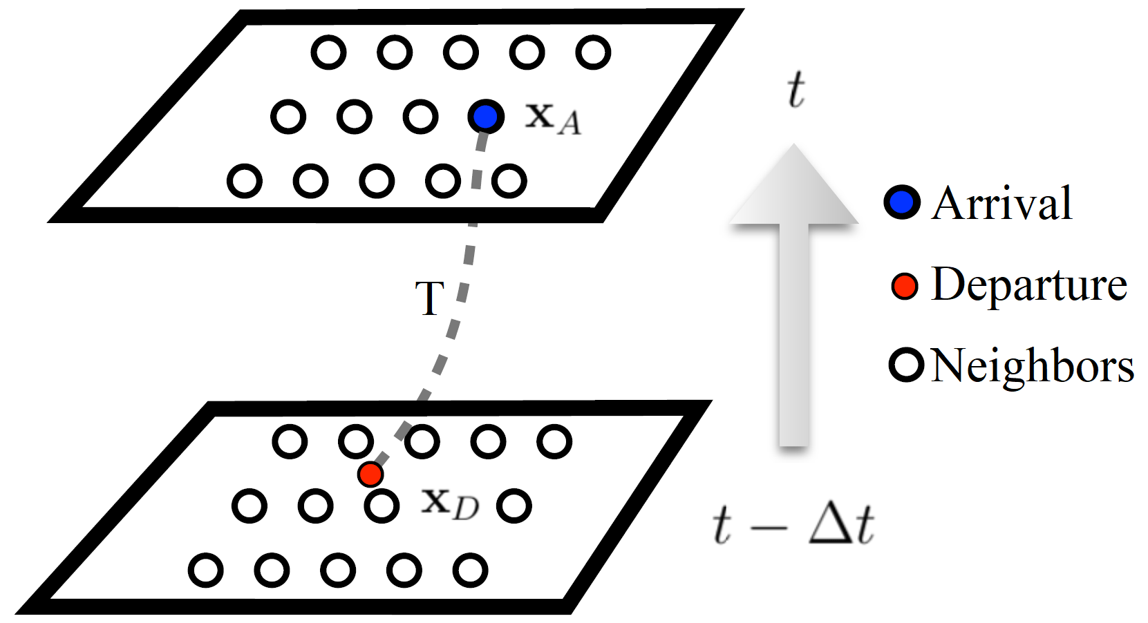
Here, A:(Xt) and $D:\left(\mathbf{X}-\mathrm{\Delta }\mathbf{X},t-\mathrm{\Delta }t\right)$ correspond to the arrival and departure positions of flow trajectories, respectively (see Fig. 1).

Figure 1 Procedure of time marching in semi-Lagrangian scheme.

In the second step, we add the forcing term to the intermediate solution to find the results at the present time step:

$$\begin{array}{}\text{(8)}& {\mathrm{\varnothing }}_A={\mathrm{\varnothing }}_A^{\ast }+\mathrm{\Delta }tP.\end{array}$$

In the semi-Lagrangian method, the most challenging part is calculating the value of the variables at the departure point ${\mathbf{X}}_D=(x_D,y_D,z_D)$. To accomplish this, first we need to find the position X_D by moving back along the flow trajectory T arriving at X_A:

$$\begin{array}{}\text{(9)}& {\mathbf{X}}_D={\mathbf{X}}_A-\underset{t-\mathrm{\Delta }t}{\overset{t}{\int }}\mathit{V}\left(\mathrm{X}\left(\mathit{\tau }\right),\mathit{\tau }\right)\mathrm{d}\mathit{\tau }.\end{array}$$

By using an averaging procedure for the integral of velocity on the right-hand side of Eq. (9), this equation can be written as follows:

$$\begin{array}{}\text{(10)}& {\mathbf{X}}_D={\mathbf{X}}_A-(B{V}_A+\left(\mathrm{1}-B\right)V_D),\end{array}$$

where B≥0.5 is an off-centering weight. Because the position of the departure point (X_D) does not necessarily coincide with a grid point, the use of an interpolation scheme is required to transfer data from the Eulerian grid to the departure point (Williamson and Rasch, 1989; Purser and Leslie, 1991). Lagrange interpolation is used in GEM:

$$\begin{array}{}\text{(11)}& {\mathrm{\varnothing }}_A^{\ast }=\sum _l{w}_l{\mathrm{\varnothing }}_l^{t-\mathrm{\Delta }t},\end{array}$$

where l represents the index of neighbor grid points surrounding the departure point, and w_l denotes the interpolation weights. The cubic interpolation currently used in GEM uses 64 neighbor cells, i.e., 4 grids in each direction, to achieve fourth-order spatial accuracy. Below, we explain the Mortezazadeh and Wang (2017) method to generate a high-order-accurate semi-Lagrangian scheme by using only 27 neighbor cells that has the same accuracy as a SL method based on the standard cubic interpolation and which can also lead to a faster interpolation process.

For the sake of illustrating how the sweep method works, we use the 1D discretization of the equations based on the uniform grid spacing size of Δx that is shown in Fig. 2.

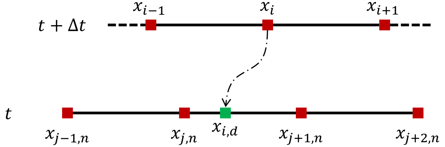
Figure 2 One-dimensional computational stencil diagram of neighborhoods near the departure point.

As mentioned before, the cubic Lagrange interpolation scheme uses four grid neighbors, along the 1D direction, to calculate ∅_D at the departure point x_i,D, i.e., x_l−1, x_l, x_l+1, and x_l+2. Here i is the index of arrival cells or Eulerian grid points. Note that here using the Lagrange interpolation scheme, we can construct a prediction function $\widehat{\mathrm{\varnothing }}\left(x_{i,}D\right)$ from the exact solution of ∅(x_i,D) within the cell [x_l, x_l+1]. The error in cubic interpolation can be expressed as follows:

$$\begin{array}{}\text{(12)}& \begin{array}{rl}{E}_{\mathrm{Cubic}}& =\mathrm{\varnothing }\left(x_{i,D}\right)-\widehat{\mathrm{\varnothing }}\left(x_{i,D}\right)\\ & ={\displaystyle \frac{\mathrm{1}}{\mathrm{4}\mathrm{!}}}{\mathrm{\varnothing }}^{\left(\mathrm{4}\right)}\left(x_{i,D}\right)\times \prod _{l-\mathrm{1}}^{l+\mathrm{2}}\left(x_{i,D}-x_l\right)\\ & =O\left(\mathrm{\Delta }{x}^{\mathrm{4}}\right).\end{array}\end{array}$$

Sweep interpolation is an integration of two third-order backward and forward interpolation steps that are used successively in two time steps. In the following, we show how sweep interpolation can achieve almost the similar accuracy to cubic interpolation by using fewer grid neighbors. Equation (13) shows the numerical errors in third-order backward (E_B) and forward (E_F) polynomial interpolation schemes:

$$\begin{array}{}\text{(13)}& \begin{array}{rl}{E}_{\mathrm{B}}& ={\displaystyle \frac{\mathrm{1}}{\mathrm{3}\mathrm{!}}}{\mathrm{\varnothing }}^{\left(\mathrm{3}\right)}\left(x_{i,D}\right)\times \prod _l^{l+\mathrm{2}}\left(x_{i,D}-x_l\right)=-O\left(\mathrm{\Delta }{x}^{\mathrm{3}}\right)\\ E_{\mathrm{F}}& ={\displaystyle \frac{\mathrm{1}}{\mathrm{3}\mathrm{!}}}{\mathrm{\varnothing }}^{\left(\mathrm{3}\right)}\left(x_{i,D}\right)\times \prod _{l-\mathrm{1}}^{l+\mathrm{1}}\left(x_{i,D}-x_l\right)=O\left(\mathrm{\Delta }{x}^{\mathrm{3}}\right).\end{array}\end{array}$$

From Eq. (13) we find that the numerical error for the two interpolation steps is almost the same but with opposite sign. While use of either the backward or forward interpolation scheme after two time steps can generate $E_{\mathrm{B}},\mathrm{2}\times \mathrm{\Delta }t=\mathrm{2}\times E_{\mathrm{B}}$, using third-order backward and forward interpolation successively in two time steps can eliminate the third-order numerical errors O(Δx³) and produce an O(Δx⁴) interpolation error.

$$\begin{array}{}\text{(14)}& E_{\mathrm{2}\times \mathrm{\Delta }t}=E_{\mathrm{B}}+E_{\mathrm{F}}\approx O\left(\mathrm{\Delta }{x}^{\mathrm{4}}\right).\end{array}$$

Here the analysis of the numerical errors is shown by assuming a constant Δx (uniform grids) in the above equations, but it is also valid for non-uniform grids (Mortezazadeh and Wang, 2017). Although, as shown above, the truncation errors in two backward and forward steps nearly cancel out to produce a total truncation error with a leading term that is proportional to the fourth power of the grid increment, the actual numerical accuracy of its implementation in SL schemes needs to be assessed. In the next section, we assess how the sweep interpolation approach can control the error after every two time steps in the SL scheme in GEM. In this study, sweep interpolation is used not only for semi-Lagrangian advection, but also for exchanging the data between yin and yang grids in GEM. In the following, we investigate the performance of the model by solving three benchmarks and an ozone prediction case.

3 Validation

The objective of this evaluation is to illustrate the feasibility of implementing the sweep interpolation within the GEM model to replicate the forecast results achieved by the GEM configuration based on cubic interpolation. The evaluation has been done by running one 2D case and three 3D cases to represent the accuracy and performance of the proposed method. Error analysis is performed to show that semi-Lagrangian with sweep interpolation can provide similar results to cubic interpolation in a more cost-effective manner.

3.1 Two-dimensional vortex

The 2D vortex is a conventional benchmark which is used here to compare the accuracy of the sweep interpolation with the cubic interpolation. This case consists of a scalar field that is deformed by two static vortices centered at the geographical poles (Nair and Machenhauer, 2002). The flow field utilized in this benchmark is positive definite. The spatial resolution used in both horizontal directions is approximately 105 km, and a time step of 7200 s is employed, which yields a maximum Courant number value of 0.85426. By considering (λ,φ) as the rotated coordinate system, North Pole location λ₀,φ₀, and an angular velocity ω, we can write the rotation of the scalar field as

$$\begin{array}{}\text{(15)}& \begin{array}{rl}& {\displaystyle \frac{\mathrm{d}\mathit{\lambda }}{\mathrm{d}t}}=\mathit{\omega }\\ & {\displaystyle \frac{\mathrm{d}\mathit{\phi }}{\mathrm{d}t}}=\mathrm{0}.\end{array}\end{array}$$

The normalized tangential velocity of the vortex is defined as

$$\begin{array}{}\text{(16)}& V_t={\displaystyle \frac{\mathrm{3}\sqrt{\mathrm{3}}}{\mathrm{2}}}{\mathrm{sech}}^{\mathrm{2}}\left(r\right)\tanh \left(r\right),\end{array}$$

where r=r₀cos φ is the radius of the vortex, and r₀ is a constant. Then, the angular velocity ω is defined as

$$\begin{array}{}\text{(17)}& \mathit{\omega }\left(\mathit{\phi }\right)=\left\{\begin{array}{ll}\mathrm{0}& \text{ if }r=\mathrm{0}\\ \frac{V_t}{r}& \text{ if }r\ne \mathrm{0}\end{array}\right..\end{array}$$

The analytical solution of this case at time t is available in the reference (Nair and Machenhauer, 2002). Figure 3a shows error in the tracer at day 12. It can be seen that the error distribution inside the domain is almost similar for both schemes.

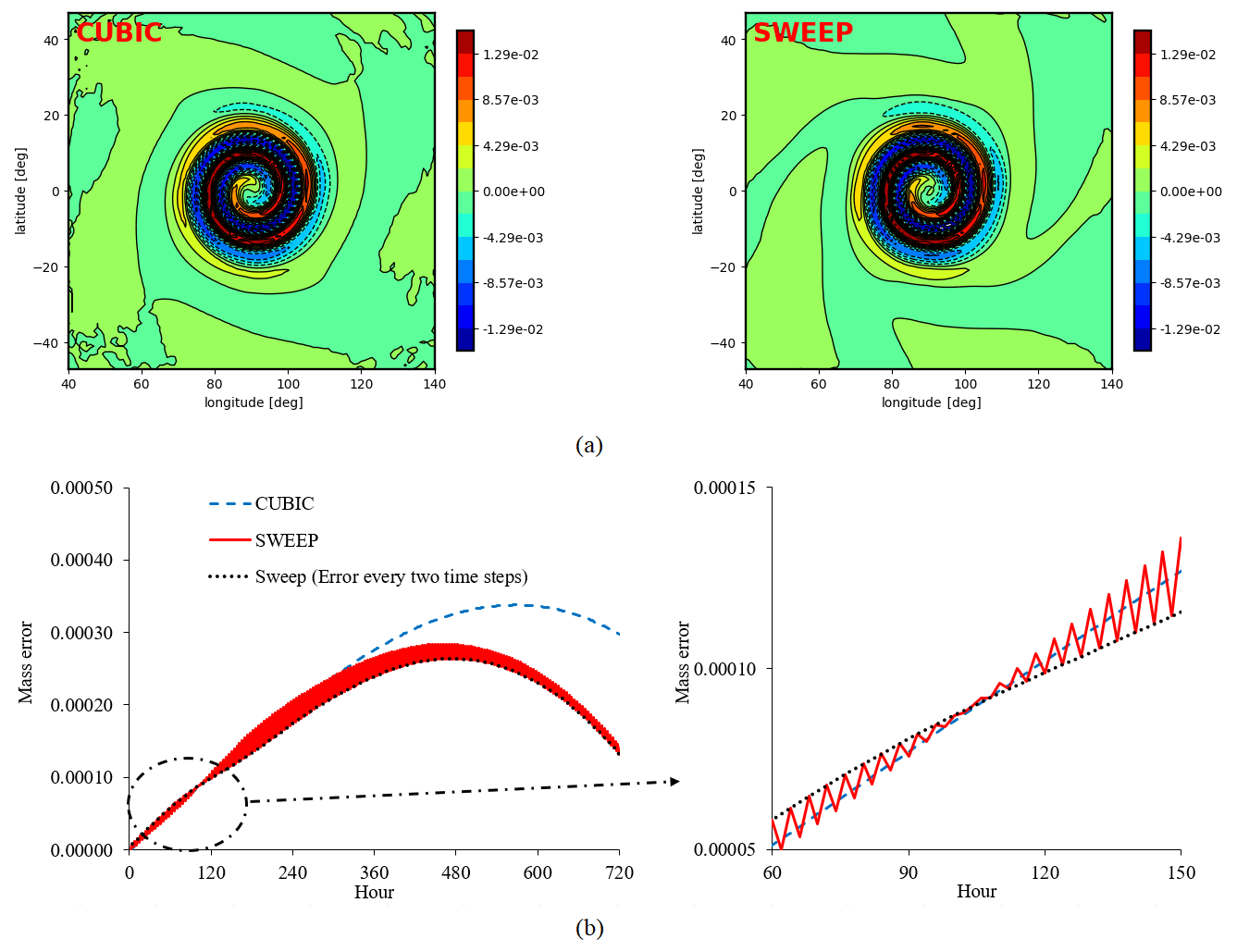
Figure 3 Two-dimensional vortex: (a) horizontal cross-section of errors in tracer distribution at day 12, (b) mass conservation error (%) over a 1 month period.

Figure 3b shows the mass error over 1 month. This figure shows an oscillation in mass error, calculated by sweep interpolation, which comes from the inherent behavior of sweep interpolation to control the growth of numerical error over two successive time steps. The dotted black line in Fig. 3b shows the mass error after each two time steps, which represents the impact of sweep interpolation to reduce the error. This line represents the impact of sweep interpolation to reduce the error. The main reason of choosing the 2D case was showing the oscillation in the mass error for sweep interpolation. In this case, the oscillation is obvious and helps explain the behavior of sweep interpolation. The same behavior has been seen in the other test cases (see next sections). For this case, the normalized infinity norm error ($E_{\mathrm{\infty }}=\frac{\max \mathrm{|}\text{cubic-sweep}\mathrm{|}}{\max \mathrm{|}\text{cubic}\mathrm{|}})=\mathrm{0.001}$. Figure 3a shows that the error distribution associated with the sweep interpolation is less noisy compared with the cubic interpolation error, especially outside the vortex region, which could be explained by the fact that the lower-order Lagrange interpolation used in the sweep algorithm generates less spurious oscillations compared to the standard cubic interpolation.

3.2 Hadley-like meridional circulation

The Hadley-like meridional circulation test case is used to emphasize the solution of horizontal-vertical coupling (Ullrich et al., 2013). The tracer field consists of a single layer, which is deformed over the duration of 24 h. At the end, the tracer field returns to its original configuration. Meridional and vertical velocity fields for this test case are specified as

$$\begin{array}{}\text{(18)}& {\displaystyle }u\left(\mathit{\lambda },\mathit{\phi },z,t\right)=u_{\mathrm{0}}\cos \mathit{\phi }\text{(19)}& {\displaystyle }v\left(\mathit{\lambda },\mathit{\phi },z,t\right)={\displaystyle \frac{a{w}_{\mathrm{0}}\mathit{\pi }{\mathit{\rho }}_{\mathrm{0}}}{K{z}_{\mathrm{top}}\mathit{\rho }}}\cos \mathit{\phi }\sin \left(K\mathit{\phi }\right)\cos \left({\displaystyle \frac{\mathit{\pi }z}{z_{\mathrm{top}}}}\right)\cos \left({\displaystyle \frac{\mathit{\pi }t}{\mathit{\tau }}}\right)\text{(20)}& {\displaystyle }\begin{array}{rl}w\left(\mathit{\lambda },\mathit{\phi },z,t\right)& ={\displaystyle \frac{w_{\mathrm{0}}{\mathit{\rho }}_{\mathrm{0}}}{K\mathit{\rho }}}\left(-\mathrm{2}\sin \left(K\mathit{\phi }\right)\sin \mathit{\phi }\right.\\ & \left.+K\cos \mathit{\phi }\cos \left(K\mathit{\phi }\right)\right)\sin \left({\displaystyle \frac{\mathit{\pi }z}{z_{\mathrm{top}}}}\right)\cos \left({\displaystyle \frac{\mathit{\pi }t}{\mathit{\tau }}}\right),\end{array}\end{array}$$

where ρ₀, K=5, z_top=12 000 m, w₀=0.15 m s⁻¹, u₀=40 m s⁻¹, a and τ=86 400 s are the density at the surface, number of overturning cells, height position of the model top, reference vertical velocity, reference zonal velocity, reference earth radius, and period of motion. The horizontal spatial resolution and time step used in this example are, respectively, 205 km and 3600 s, which yields a horizontal Courant number (CFL) of 5.0.

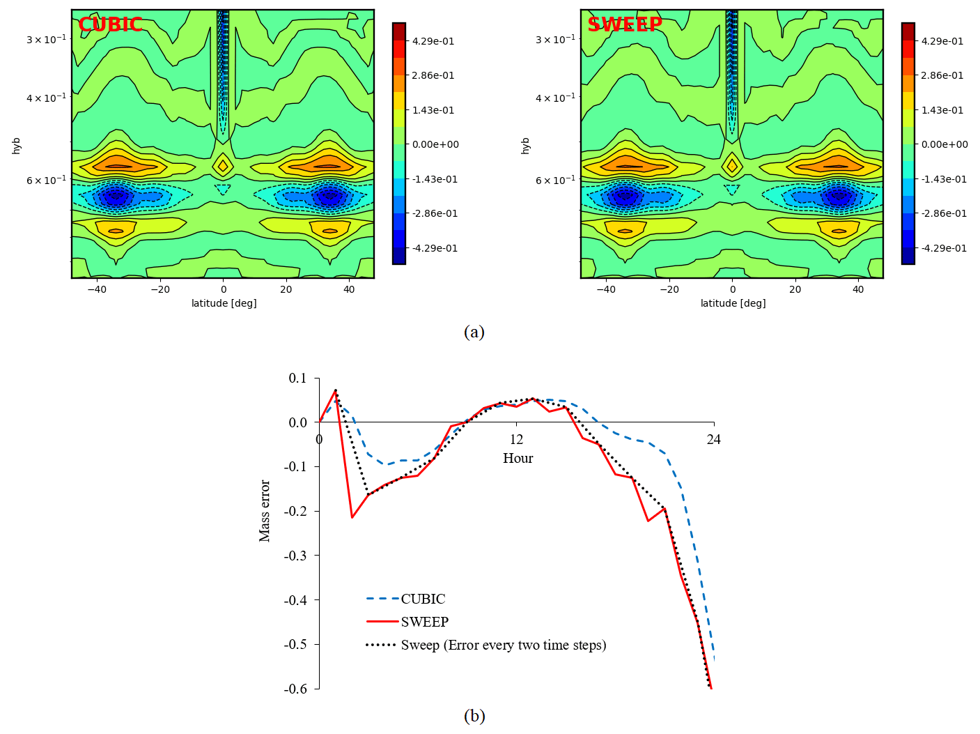
Figure 4 Hadley-like meridional circulation: (a) vertical cross-section of errors in tracer at day 1, (b) mass conservation error (%) over 1 d.

Figure 4a presents the meridional cross-sections of the errors in the tracer solution after a 24 h integration period. The results show that sweep interpolation generates a solution (right panel) that is similar to the one generated with the fourth-order-accurate cubic interpolation (left panel). Figure 4b shows the evolution of the error in the mass conservation (%) over the same 24 h period corresponding to both interpolations. The evolution in both solutions remains almost the same for both sweep and cubic interpolations. Note that here we can see the oscillations in error for the sweep interpolation scheme. As explained in the previous section, this shows how sweep interpolation can control the error growth over each two time steps. Here, the normalized infinity norm error is E_∞=0.03.

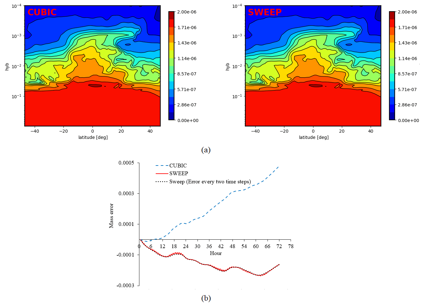
Figure 5 CH₄ Forecasts: (a) meridional cross-sections at 180^∘ longitude at the end of day 1, (b) normalized mass error (%) over 3 d forecast.

3.3 Atmospheric methane-like tracer

In this test case, we compare 48 h forecasts of atmospheric methane (CH₄) like passive tracer (without chemical productions and sinks) using sweep interpolation and cubic interpolation. These experiments were performed with the global version of the GEM NWP model using a 30 min time step and 105 km horizontal resolution, resulting in a maximal Courant number of 4.7. The height of the model top was chosen to be at 0.1 hPa, and 84 vertical levels were used. The vertical grid resolution is non-uniform as a result of the choice of vertical coordinate, which is based on the logarithm of the hydrostatic pressure (Husain et al., 2020). The methane-like experiment was initialized from a climatology based on a multi-year simulation performed with the GEM model. The model employs a simplified approach, in which methane production and loss are predetermined based on present-day conditions (Prather et al., 2012). Figure 5a presents meridional cross-sections of CH₄ at the end of day 1. Solutions from both interpolators look qualitatively the same, and the sweep interpolation provides acceptable results in comparison with cubic interpolation. Figure 5b shows the mass error over 24 h. It shows that both cubic and sweep interpolations could control the error and keep its range below 0.005 % after 48 time steps of simulation. Here, the normalized infinity norm error is E_∞=0.018.

Although sweep interpolation was able to better control the mass error growth over the simulation time compared to the cubic interpolation for this case, it is not necessarily expected to perform better in all cases. Based on our discussion in the previous section, we expect sweep interpolation to provide almost the same accuracy as cubic interpolation. This is supported by Fig. 5b, which shows that sweep and cubic interpolations produce mass errors that are of the same order of magnitude. However, since both methods rely on different finite-difference approximations, we expect to see differences in the evolutions of their respective error trends, which is confirmed by the results of Fig. 5b.

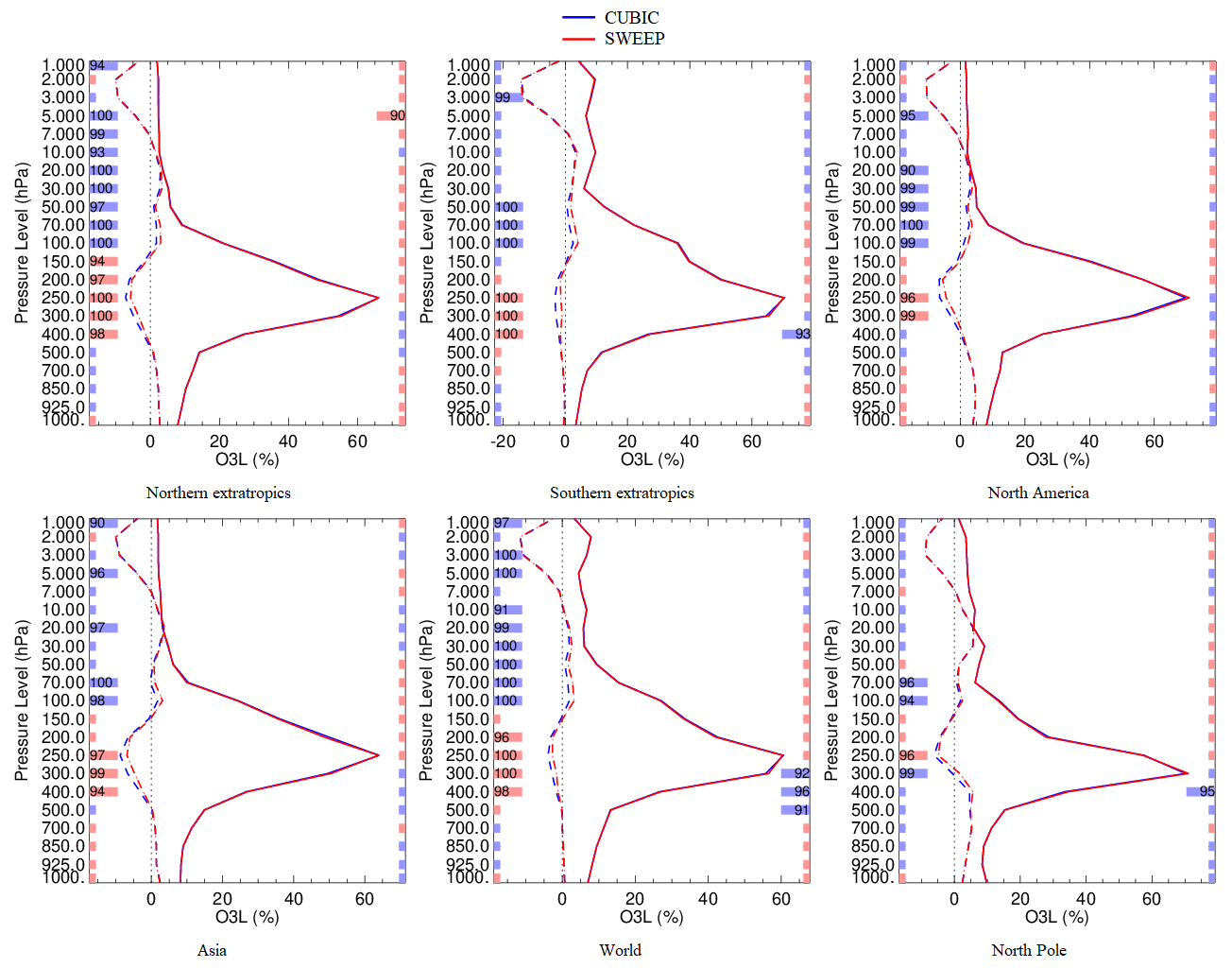
Figure 6 The bias (dashed line) and standard deviation (solid line) relative to Global Deterministic Prediction System (GDPS) analyses (%) for ozone forecasts at 240 h lead time from 13 June to 31 August 2019. Boxes on the left (right) indicate statistical significance levels for biases (standard deviation). Red (blue) boxes mean that the experiment which includes the sweep interpolation is better (worse). Small boxes mean that differences between both experiments are not statistically significant at the 90 % confidence level.

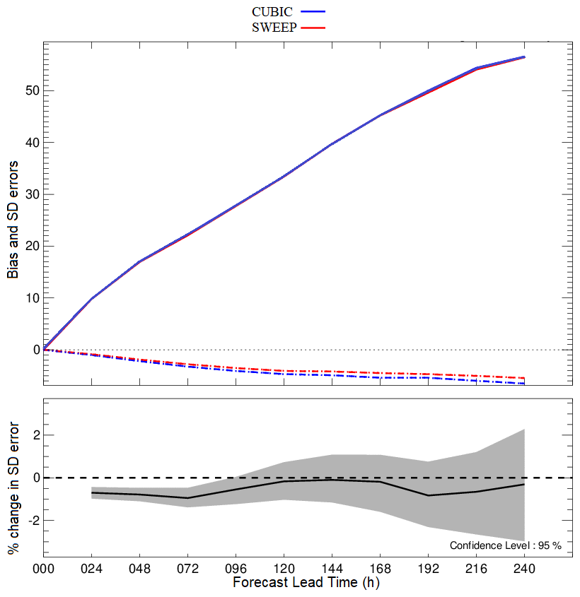
Figure 7 Standard deviation (solid line) and bias (dashed line) errors over North America for ozone at the level 200 hPa.

Figure 8 Computational time analysis based on the number of tracers.

3.4 Medium-range forecast of ozone

In the upper troposphere–lower stratosphere (UTLS) region, ozone is mainly driven by transport processes, which makes it a valuable tracer for assessing the impact of the new interpolation scheme on the transport of chemical constituents. The implementation of sweep in the ECCC GEM NWP model allowed evaluation of its impact on the ozone predictability in the context of an operational NWP system. In this experiment, an ensemble of 10 d ozone forecasts were launched every 12 h from 13 June to 31 August 2019 using the global version of the GEM NWP model. These forecasts were performed at 15 km horizontal resolution on 84 vertical levels with a lid at 0.1 hPa and using a 450 s time step. The model included a prognostic representation of stratospheric ozone based on a linearized chemistry scheme which did not interact with the radiation (de Grandpré et al., 2016). Ozone forecasts have been evaluated at different lead times against operational analyses generated by the Global Deterministic Prediction System (Charron et al., 2012). This evaluation was done throughout the tropospheric and stratospheric regions in various areas, including the northern and southern extratropics, North America, Asia, the Arctic, and the Antarctic.

The results from two interpolations, i.e., cubic and sweep interpolations, at different locations over the global experiments demonstrate good agreement between sweep interpolation and cubic interpolation. The two main metrics of the statistical accuracy, bias and standard deviation, are used to show the differences between the two experiments. In the following figures (Figs. 6 and 7), solid and dashed lines represent the standard deviation and bias metrics, respectively. Figure 6 represents the average of all 10 d lead time forecasts in the simulation time period. This figure shows that the standard deviations for both experiments are almost the same, but some minor deviations can be seen in the bias. The bias for ozone variation along the vertical direction is similar for both experiments in the lower part of the troposphere (>500 hPa) and in the upper stratosphere (<50 hPa). The smaller concentration of ozone in these two regions accounts for the absence of sharp gradients in the vertical error profiles. The large maximum in the standard deviation around 250 hPa is associated with the transport of ozone across the tropopause. This process is sensitive to the choice of interpolation scheme, and the results highlight its impact on stratosphere–troposphere exchange processes throughout the entire upper troposphere and lower stratosphere region between 400 and 50 hPa. In this region, a minor deviation of bias error can be seen between sweep interpolation and cubic interpolation, but this deviation is small and not significant (see Fig. 6).

Figure 7 shows the evolution of the bias and standard deviation as a function of lead time for the North America region at the 200 hPa level, which corresponds to the region where both quantities vary the most abruptly along the vertical direction. The upper panel shows the standard deviation and bias errors over 10 d prediction. It demonstrates that sweep interpolation is characterized by the same error growth as the cubic interpolation. The figure also shows some improvement in the bias error that was obtained by using sweep interpolation. One possible explanation for this phenomenon is that the lower-order Lagrange interpolations used in the backward and forward steps of the sweep interpolation tend to generate less oscillation and dispersion errors than the standard fourth-order-accurate cubic interpolation. To confirm this explanation, further study needs to be done, which is out of the scope of this paper.

4 Impact of number of tracers on computational time

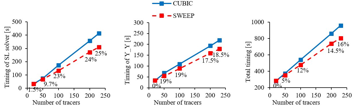
In the following, we investigate the impact of increasing the number of tracers on the timing of the cubic interpolation process compared to sweep interpolation. We use the benchmark test case 2 (i.e., 24 h forecasts of chemical CH₄ tracer) from the previous section and add additional tracers to the experiment. Note that in GEM we use cubic interpolation not only for the advection solver but also for exchanging the data between the yin and yang grid (Qaddouri and Lee, 2011). In this study, we also implemented sweep interpolation into yin and yang exchange of data. Figure 8 shows the impact of sweep interpolation on the timing of the advection process, the exchange of data between the yin and yang subgrids, and the total timing of the simulation. The numbers shown in Fig. 8 correspond to (time_cubic − time_sweep) $/$ time_cubic × 100. It is demonstrated that by increasing the number of tracers, the percentage of computational time saving increases for the semi-Lagrangian operation, yin and yang exchange, and the total timing of the simulation. When using only 20 tracers, the performance of sweep interpolation is almost the same as cubic interpolation. However, when the number of tracers is increased to 230, sweep interpolation can reduce the computational cost of simulation in the advection step by 25 %. The sweep interpolation reduction in yin and yang exchange is about 18.5 %, and its impact on the total timing of the simulation is about 16 %.

5 Conclusion

In this study, we implemented the sweep interpolation scheme (an integration of two third-order backward and forward interpolation steps) into ECCC's GEM model. Two theoretical benchmarks and a global ozone forecast experiment were used to investigate the performance of the model. Based on the results, the sweep interpolation results are in good agreement with those from the standard cubic interpolation but achieved at a lower computational cost.

The main benefit of using sweep interpolation in GEM is its lower computational cost compared to the cubic interpolation. By using this interpolation, we can reduce the timing of semi-Lagrangian interpolation, yin-yang exchange, and the total wall clock time of the simulation up to 25 %, 19 %, and 15 %, respectively, for the experiments with around 250 tracers. Additionally, this replacement is very simple, with minimum modifications required in the model. Sweep interpolation is suitable to be implemented in other NWP models which also rely on a SL approach and polynomial interpolation schemes.

Although sweep interpolation is developed based on third-order backward and forward Lagrange interpolation schemes, it can control the growth of the mass conservation error over the forecast lead time in a way that agrees very closely with the error growth of the standard cubic interpolation. The ozone forecasting experiment using the global version of the GEM model shows that the sweep interpolation has a small impact on the ozone distribution along the vertical direction. The impact is the most significant in the tropopause region, where transport processes play a significant role. The overall impact of the new scheme on model biases and standard deviations was evaluated at different lead times, which shows that the overall performance of the ozone forecasting system has not suffered from the use of a faster interpolation approach. In some cases, we found that sweep interpolation can perform better and reduce the numerical errors compared to those of the standard cubic interpolation. The impact on biases in ozone experiments generally increases with longer lead time and is larger over some regions driven by transport processes. This improvement is likely related to the lower oscillations generated by the lower order of Lagrange interpolation schemes used in sweep compared to the standard cubic interpolation, but this needs to be further investigated in a future study.