Bergen metrics: composite error metrics for assessing performance of climate models using EURO-CORDEX simulations

Error metrics are useful for evaluating model performance and have been used extensively in climate change studies. Despite the abundance of error metrics in the literature, most studies use only one or two metrics. Since each metric evaluates a specific aspect of the relationship between the reference data and model data, restricting the comparison to just one or two metrics limits the range of insights derived from the analysis. This study proposes a new framework and composite error metrics called Bergen metrics to summarize the overall performance of climate models and to ease interpretation of results from multiple error metrics. The framework of Bergen metrics are based on the p norm, and the first norm is selected to evaluate the climate models. The framework includes the application of a non-parametric clustering technique to multiple error metrics to reduce the number of error metrics with minimum information loss. An example of Bergen metrics is provided through its application to the large ensemble of regional climate simulations available from the EURO-CORDEX initiative. This study calculates 38 different error metrics to assess the performance of 89 regional climate simulations of precipitation and temperature over Europe. The non-parametric clustering technique is applied to these 38 metrics to reduce the number of metrics to be used in Bergen metrics for eight different sub-regions in Europe. These provide useful information about the performance of the error metrics in different regions. Results show it is possible to observe contradictory behaviour among error metrics when examining a single model. Therefore, the study also underscores the significance of employing multiple error metrics depending on the specific use case to achieve a thorough understanding of the model behaviour.

1 Introduction

Climate models are important tools for predicting and understanding climate change and climate processes (Kotlarski et al., 2014; IPCC, 2021a, b; Mooney et al., 2022). In the context of climate studies, climate model evaluation is essential for identifying models that poorly simulate the climate system and for the ranking of climate models (Randall et al., 2007; Flato et al., 2013). The main purpose of climate model evaluation is twofold: firstly to ensure that the models are reproducing key aspects of the climate system and secondly to understand the limitations of climate projections from the models. This ensures proper interpretation and application of climate models and any climate projections produced by them. The performance of climate models is quantified by different error metrics such as root mean square error and bias, which assess the agreement between the climate model data and reference data (e.g. gridded observational products, station data, reanalyses, or satellite observations). As the number of climate models has increased, the study of error metrics has become increasingly important. There are several error metrics available to evaluate the performance of climate models (Jackson et al., 2019), and the selection of an appropriate metric remains a topic of debate in the literature. For instance, Willmott and Matsuura (2005) advocate for mean absolute error (MAE) over root mean squared error (RMSE), as the latter is not an effective indicator of average model performance. In contrast, Chai and Draxler (2014) contend that RMSE is superior to MAE when errors follow a Gaussian distribution. Different error metrics are available in the literature, and each has a specific framework according to its purpose (Rupp et al., 2013; Pachepsky et al., 2016; Baker and Taylor, 2016; Collier et al., 2018; Jackson et al., 2019). For example, root mean square error compares the amplitude difference between modelled and reference data, while the correlation coefficient compares the phase difference between modelled and reference data. Depending on the specific error, the error metrics can be categorized into different classes; the most popular classes are accuracy, precision, and association. Accuracy measures the degree of similarity between climate model data and reference data. An extremely high accuracy indicates that the model has less error magnitude of any type and testing the model with other error metrics adds little value (Liemohn et al., 2021). However, if a model has moderate to low accuracy, testing the model with other metrics can reveal other similarities and dissimilarities between model data and reference data. Root mean square error and mean square error are the most used accuracy metrics to evaluate climate models (Watt-Meyer et al., 2021; Wehner et al., 2021; He et al., 2021), even though the metrics cannot reveal whether the model is under- or over-predicting the observations. Precision metrics quantify the degree of similarity in the spread of the data. A robust and commonly used metric for assessing the precision of model data is the ratio of or difference in standard deviation between modelled data and reference data (van Noije et al., 2021; Wood et al., 2021; Wehner et al., 2021). Finally, association metrics measure the degree of the phase difference between modelled data and observed data. Phase difference is important in climate studies as it affects the initiation and termination time of a season of climate variables. One metric that is extensively used to measure the association is the correlation coefficient (Richter et al., 2022; Bellomo et al., 2021; Yang et al., 2021). Liemohn et al. (2021) have described various other major categories of metrics, and they suggest that assessment of models should not be restricted to one or two error metrics. Interested readers can follow the citations to read in detail about the discussed metrics.

In addition to this, researchers have employed various characteristics of climatic parameters as measures to assess and compare climate models with observed datasets. Metrics encompassing the frequency of days with precipitation over 1 mm and over 15 mm, the 90 % quantile of the frequency distribution, and the maximum number of consecutive dry days, along with parameters such as daily mean, daily maximum, daily minimum, yearly maximum, length of the frost-free period, growing degree days (> 5 °C), cooling degree days (> 22 °C), heating degree days (< 15.5 °C), days with RR (> 99th percentile of daily amounts for all days), ratio of spatial variability, pattern correlation, ratio of interannual variability, temporal correlation of interannual variability, number of summer days, number of frost days, consecutive dry days, and ratio of yearly amplitudes, have been utilized for the validation of Euro-CORDEX data (Kotlarski et al., 2014; Giot et al., 2016; Smiatek et al., 2016; Torma, 2019; Vautard et al., 2021). Other studies have employed the empirical orthogonal functions (Benestad et al., 2023), structural similarity index metric (Wang and Bovik, 2002), fractions skill score (Roberts and Lean, 2008), spatial pattern efficiency metric (Dembélé et al., 2020), spatial efficiency metric (Demirel et al., 2018; Ahmed et al., 2019), and probability distribution function (Perkins et al., 2007; Boberg et al., 2009, 2010; Masanganise et al., 2014) to evaluate climate models.

There are several composite error metrics that use the modified framework of other metrics to compute the error magnitude. A widely used example of this is the Taylor diagram (Taylor, 2001), which incorporates correlation, root mean square deviation, and ratio of standard deviation. A distinguishing feature of the Taylor diagram is its ability to graphically evaluate the model performance. Another popular example is the Nash–Sutcliffe efficiency (NSE; Nash and Sutcliffe, 1970), which is a normalized form of the mean squared error to evaluate and predict the model streamflow data. Later, it was observed that NSE can be decomposed into three components which are the functions of correlation, bias, and standard deviation (Murphy, 1988; Wȩglarczyk, 1998). Other similar scores include the Kling–Gupta (K–G) efficiency (Gupta et al., 2009), which is a function of three components: ratio of model mean to observed mean, the ratio of model standard deviation to observed standard deviation, and correlation coefficient. The study of Gupta et al. (2009) argued the NSE, which has a bias component normalized by the standard deviation of the reference data, will have a low weight on the bias component if the reference data have high variability. The modified Kling–Gupta efficiency developed by Kling et al. (2012) involves the ratio of covariance instead of the ratio of standard deviation.

Both K–G efficiency and modified K–G efficiency use Euclidean distance as a basis to calculate the error magnitude of the model, and the study argued that instead of finding a corrected NSE criterion, the whole problem can be viewed from the multi-objective perspective where the three error components can be used as separate criteria to be optimized. It identifies the best models by calculating the Euclidean distance from the ideal point and then finding the model with the shortest distance. The ideal value of an error metric is obtained when the model exactly simulates the observed data. The Euclidean distance is also used by Hu et al. (2019) to develop the distance between indices of simulation and observation (DISO) metric that incorporates correlation coefficient, absolute error, and root mean squared error. The study of Hu et al. (2019) also argues that accuracy (root mean square error), bias (absolute error), and association (correlation coefficient) are the three major error classes based on which a model should be assessed, and evaluating a model using a single error metric may lead to ill-informed results. The study pointed out a few limitations of the Taylor diagram such as quantification of error magnitude and low sensitivity to small error differences by the diagram. In a comparative study, Kalmár et al. (2021) found no substantial difference between the DISO index and the Taylor diagram. However, based on quantification of error magnitude, the DISO index can be helpful.

The Euclidean distance framework has found increasing use in various fields, serving as an error function or metric in applications like model evaluation, parameter optimization, and classification problems. In essence, it calculates the straight-line distance between two points in the space, known as Euclidean distance. The Euclidean distance is essentially the second norm of a vector. Equation (1) represents the generalized form of the p norm in an n-dimensional vector space, where x_i is the vector. When p is set to 2, it transforms into the Euclidean norm.

In the context of time series data, if the vector (x_i) represents the difference between observed data (u_i) and model data (v_i), i.e. ${\mathit{x}}_i=u_i-v_i$, then d is termed the Euclidean distance metric. Here, i represents the time series data. It is important to note that root mean squared error and mean squared error are different variants of the Euclidean distance metric.

Furthermore, if the vector represents the difference between error metrics (correlation coefficient [u₁], absolute error [u₂], and root mean squared error [u₃]) and their ideal values (v_1:3), then d is referred to as the DISO index. In summary, the Euclidean distance framework offers a versatile approach applicable to various scenarios, providing valuable insights through different metrics and indices. A disadvantage of the Euclidean distance is that it suffers the curse of dimensionality (Mirkes et al., 2020; Weber et al., 1998); i.e. Euclidean distance as a dissimilarity index becomes less efficient as dimension increases. In this study, we assess the effect of the norm order on the overall error. We use different measures such as the contribution of outliers to the overall error, the difference between the maximum and minimum distances, and the average distances to compare different norms.

$$\begin{array}{}\text{(1)}& d_n(u,v)=({\sum }_{i=\mathrm{1}}^n{\left|{\mathit{x}}_i(u_i,v_i)\right|}^p{)}^{\mathrm{1}/p}\end{array}$$

This study has the following objectives:

• i.

  evaluation of 89 CMIP5-driven regional climate simulations from the Euro-CORDEX initiative using 38 error metrics;

• ii.

  clustering of error metrics to assess their performance;

• iii.

  assessment and recommendation of different p norms based on their performance;

• iv.

  formulation of a composite metric using the optimal norm.

2 Data and study area

We focus on Europe due to the widespread availability of a large ensemble of high-resolution (0.11°) regional climate simulations. In this study, we use 89 regional climate model (RCM) simulations from Euro-CORDEX to study the behaviour of different error metrics. The Euro-CORDEX dataset provides both precipitation and temperature data at 0.11° grid resolution. The monthly data from 1975 to 2005, which are available in all the RCM simulations, have been used to calculate the index. Table S1 in the Supplement provides an overview of the global climate models (GCMs) downscaled by the different RCMs. Table S2 provides an overview of the RCMs and assigns a number (Column 1) to each RCM which is used to identify RCMs in plots that have limited space for labels.

For reference data, both precipitation and temperature data are obtained from the E-OBS dataset. The study utilized the 0.25° grid resolution dataset to meet the specific requirements of the project. However, users can choose datasets of different resolutions based on their study needs for climate model validation. To facilitate the comparison of model data with the reference data, all datasets need to be on a common grid. In this study, we remapped the RCM data onto the coarser 0.25° grid of E-OBS.

The study uses the eight sub-regions of Europe defined by Christensen and Christensen (2007) – British Isles, Iberian Peninsula, France, mid-Europe, Scandinavia, Alps, Mediterranean, and Eastern Europe – to conduct analysis in more homogeneous areas.

3 Methodology

This section outlines the framework for clustering error metrics and provides a brief overview of their characteristics. Additionally, the section describes the proposed metric's framework.

3.1 Error metrics

Error metrics play a crucial role in climate change studies, serving as essential tools to quantify the disparities between modelled and reference data over time series. Each error metric is designed to capture specific aspects of the relationship between model data and reference data, as discussed in the Introduction section. To gain insight into the performance of error metrics, we have analysed Euro-CORDEX precipitation data and examined the differences in ranking of 89 GCM-driven regional climate simulations using 38 error metrics. The list of error metrics is provided in Table S3, and the details of all 38 error metrics have been provided in Jackson et al. (2019). All 89 models are ranked based on their performance using the 38 error metrics. The average (r_M,mean; Eq. 2) and maximum (r_M,max; Eq. 3) rank differences are then calculated at each grid point. The former is the mean of all the pairwise rank differences, while the latter is the maximum of all the pairwise rank differences. These calculations allow us to understand the performance of different error metrics and the extent of the disparity in ranking of the climate models.

$$\begin{array}{}\text{(2)}& {\displaystyle }{r}_{\mathrm{M},\mathrm{mean}}={\mathit{\mu }}_{\mathrm{g}}\left(R_{\mathrm{M},k}-R_{\mathrm{M},i}\right)\text{(3)}& {\displaystyle }{r}_{\mathrm{M},\max }=\underset{\mathrm{g}}{max}(R_{\mathrm{M},k}-M_{\mathrm{M},i})\end{array}$$

R_M,k and R_M,i are the rank assigned to model M by the kth and ith error metrics, respectively. We have provided Table 1 as an example for better understanding the notations. If there are three climate models (M1, M2, and M3) as shown in Table 1, all the models have been assigned a number (first column), and the order must not change throughout the study. R_M,k and R_M,i for model M1 are 2 and 3, respectively. k varies from 1 to N_E−1, and i varies from k+1 to N_E, where N_E is the total number of error metrics. The difference in ranking is calculated for all possible combinations of error metrics. μ_g() and max_g() are the mean and maximum operator, respectively, which is applied across all the grid points (g:$\mathrm{1},\mathrm{2},..,$gd), and gd is the total number of grid points, which is 11 370 in this study. Figure 1 demonstrates that different error metrics used to assess climate models result in significantly different ranking orders. The average of r_M,mean across all the grid point varies from 16 to 26, whereas the average of r_M,max varies from 40 to 70. The results indicate significant differences in the ranking of the climate models by different error metrics. The disparity in ranking order may be due to the distinctive error targeted by each metric, as discussed in the Introduction section.

Table 1 Example of ranking order.

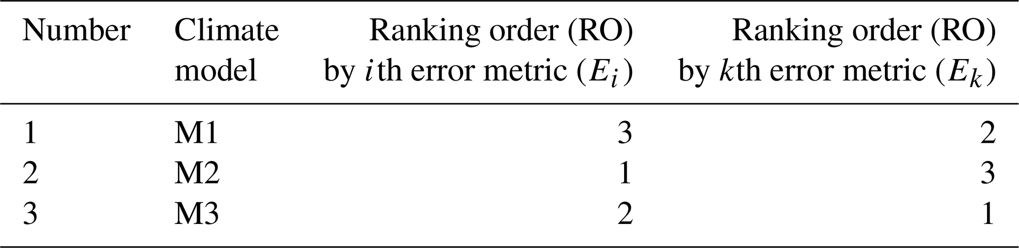
Figure 1 Box plot of average rank difference (first column, a, c) and maximum rank difference (second column, b, d) for precipitation (Pr; first row, a, b) and temperature (T; second row, c, d) over all the grid points in European region.

This study assumes that all the errors are important and that it may be necessary to evaluate model performance using multiple metrics. To achieve independence among the metrics, the study has attempted to cluster the error metrics based on model performance. This classification would enable different clusters to have unique characteristics, and metrics within the same cluster would produce similar results, whereas those from different clusters would yield different ranking orders. In summary, the study proposes that using multiple error metrics and clustering them based on performance could improve the understanding and comprehensiveness of climate model analysis.

3.2 Clustering of error metrics

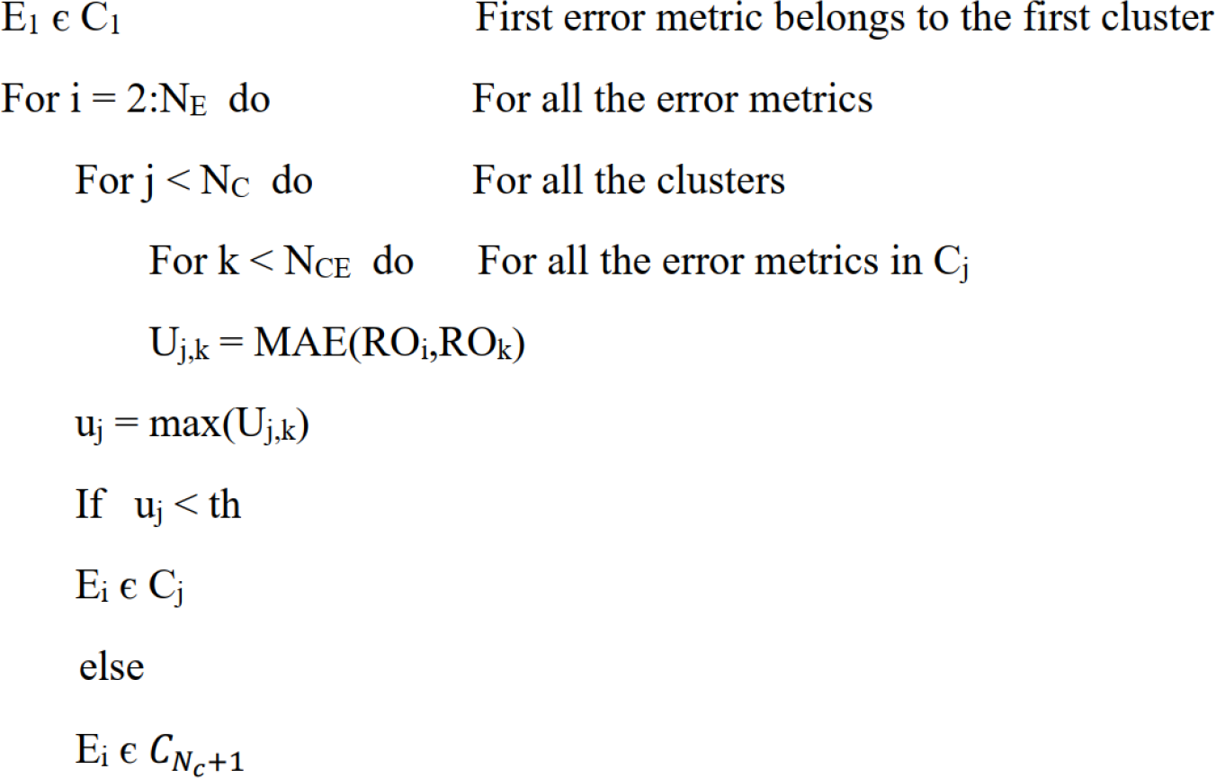
The aim of clustering error metrics is to group a set of metrics based on their similarities such that the metrics within the same cluster generate similar rankings of climate models compared to those in different clusters. This study clusters the error metrics using a non-parametric clustering approach inspired by the Chinese restaurant process (CRP; Pitman, 1995). This approach was chosen based on its performance compared to the k-means clustering approach (see Text S1 in the Supplement) and its simpler framework. The algorithm follows two fundamental principles: (i) the first error metric (E₁) forms the first cluster (C₁), and (ii) the ith error metric (E_i) is assigned to a cluster which has the maximum of all the mean absolute error (u_j) values greater than a particular threshold value (th). The clustering algorithm is presented in Algorithm 1.

Similar to the rank difference explained in the previous section, the MAE (RO_i,RO_k) between the ranking order produced by two error metrics is computed. RO is the ranking order, and it can be calculated by assigning the climate models to a number. For example, the ranking order (RO_i) by ith error metric and the ranking order (RO_k) by kth error metric are [3, 1, 2] and [2, 3, 1], respectively, in Table 1. The MAE values are calculated for all possible combinations of error metrics in a particular cluster, and the maximum of the MAE values is used to compare it to the threshold value. The exercise is repeated for all the clusters (N_C) available at that time. The number of clusters (N_C) and the number of error metrics in each cluster (N_CE) are updated for each iteration (i), and if the criteria are not satisfied, then a new cluster is formed using that error metric. The whole exercise is repeated till all the error metrics (N_E) get assigned to a cluster.

The threshold value is defined as the qth percentile of a column matrix D, where D is the collection of MAE values for all possible combinations of error metrics at all the grid points in a region. In this study, q has been assigned the value of 10 and the sensitivity of q is discussed in the Results section.

Algorithm 1 Algorithm of the non-parametric clustering for classifying the error metrics.

3.3 Proposed metric – the Bergen metrics

The clustering of error metrics guarantees that metrics in different groups produce distinct ranking orders, implying that each group targets different errors. One of the objectives of this study is to integrate different errors and create a composite error to obtain a single value. One potential solution is to use the Euclidean distance approach with different error metrics as different dimensions in the Euclidean space. To illustrate this, we employed three widely used error metrics: normalized root mean square error (RMSE), standard deviation ratio (SD), and correlation coefficient. In the Euclidean space, an ideal model that predicts the climate variable as accurately as the observed data would have values of 1, 1, and 0 for correlation coefficient, standard deviation ratio, and normalized RMSE, respectively. The coordinates of an ideal model in the Euclidean space would be (1, 1, 0), as represented by the red point in Fig. 2a. Since different models have unique coordinates based on the three metrics, these coordinates serve as possible solutions to determine the best model. If a decision is required, one approach could be to calculate the Euclidean distance from the ideal point to all points and select the point with the shortest distance (Eq. 4). The model that is closest to the ideal point, indicated by the optimal point in Fig. 2b, can be considered the best model.

$$\begin{array}{}\text{(4)}& \begin{array}{rl}& \mathrm{EDMetric}=\\ & \sqrt{\begin{array}{l}{\left(\mathrm{1}-\text{correlation coefficient}\right)}^{\mathrm{2}}+{\left(\mathrm{1}-\text{standard deviation ratio}\right)}^{\mathrm{2}}\\ +{\left(\mathrm{0}-\text{RMSE}\right)}^{\mathrm{2}}\end{array}}\end{array}\end{array}$$

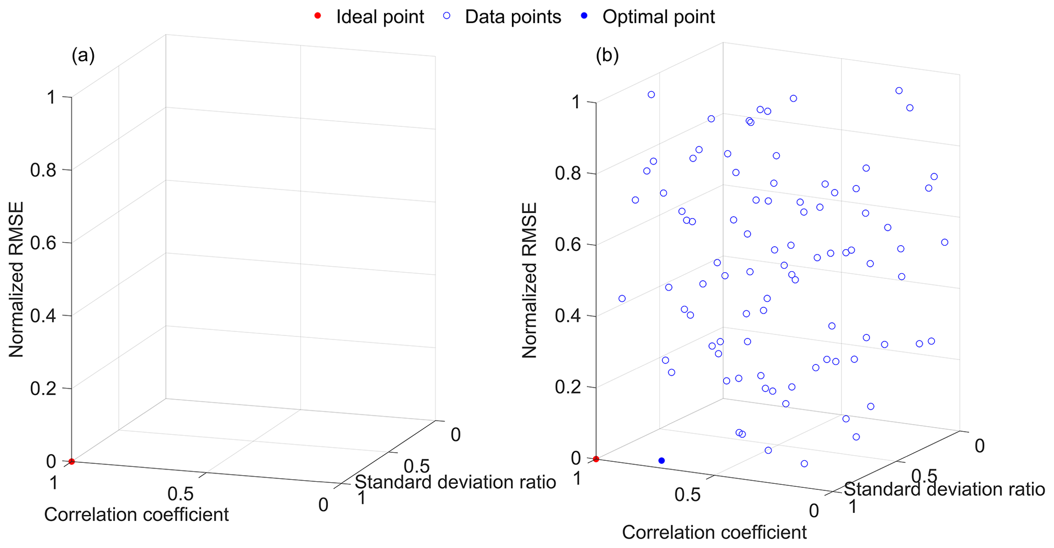
Figure 2 Example for three-dimensional (a) ideal point and (b) solution space of correlation coefficient (x axis), standard deviation (y axis), and normalized RMSE (z axis).

The Euclidian distance has several benefits that make it a popular metric, primarily its simplistic framework. However, it also has some drawbacks. The Euclidian distance, also known as L2 norm, is less effective in higher-dimensional spaces, which can lead to instability when additional error metrics are added (Weber et al., 1998; Aggarwal et al., 2001). To mitigate this issue, recent research has focused on the use of L1 norms, such as relative mean absolute error and mean absolute scaled error, which have become more popular than L2 norms like mean squared error. This approach reduces the impact of outliers in the data (Armstrong and Collopy, 1992; Hyndman and Koehler, 2006). Reich et al. (2016) found that relative MAE, based on an L1 norm, is advantageous in assessing prediction models. This study proposes a new set of metrics called the Bergen metrics (BMs), which is a generalized p-norm framework to evaluate climate models.

Figure 3 The flowchart for the calculation of Bergen metric.

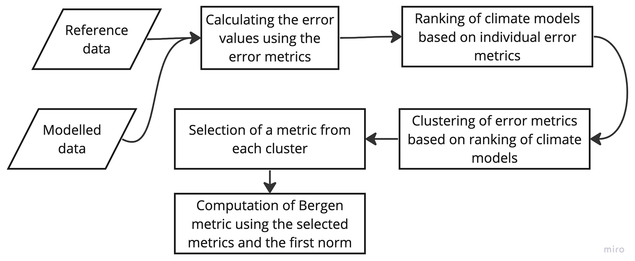
A case study has been conducted to understand the impact of different p norms on the ranking order of climate models. For this, five error metrics – RMSE, bias, correlation coefficient, standard deviation ratio, and mean ratio – have been considered (Eq. 5), and the error metrics are normalized using model data. A flowchart has been provided to illustrate the various steps involved in calculating the Bergen metrics (Fig. 3). It is important to note that Eq. (5) serves as an illustration of Bergen metrics, and users have the flexibility to include or remove metrics according to their preference. The study includes 89 RCM simulations for precipitation, and Fig. 4a shows the ranking of these models for different p norms. The lines corresponding to each model give information about the model's ranking in different norms. The results demonstrate that climate models are highly sensitive to p norms. Significant change in ranking order is observed for the first four norms. Figure 5 shows the percentage contribution of outliers to the total error magnitude for models that have outliers. A median absolute deviation technique (MAD) is used to identify outliers among the error metrics. Some of the models have only one outlier (plots with a single solid line in Fig. 5), and other models have two outliers (plots with both solid and dotted lines in Fig. 5). The percentage contribution of outliers increases as the p norm increases, consistent with previous literature (Armstrong and Collopy, 1992; Hyndman and Koehler, 2006). The study has used two parameters to indicate the capability of each norm to differentiate between climate models – mean pairwise difference in the BM and the difference between the maximum and minimum values of the BM. Figure 4b shows that both parameters decrease as the p norm increases, indicating less differentiability. The results suggest that the first norm (p=1) is the optimal norm to use as a metric in this study and will be utilized in the following analyses.

$$\begin{array}{}\text{(5)}& \begin{array}{rl}& \text{BergenMetric}\left(\mathrm{BM}\right)=\\ & \sqrt[p]{\begin{array}{l}{\left(\mathrm{0}-\mathrm{RMSE}\right)}^p+{\left(\mathrm{0}-\text{bias}\right)}^p\\ +{\left(\mathrm{1}-\text{standard deviation}\right)}^p\\ +{\left(\mathrm{1}-\text{correlation coefficient}\right)}^p+{\left(\mathrm{1}-\text{mean ratio}\right)}^p\end{array}}\end{array}\end{array}$$

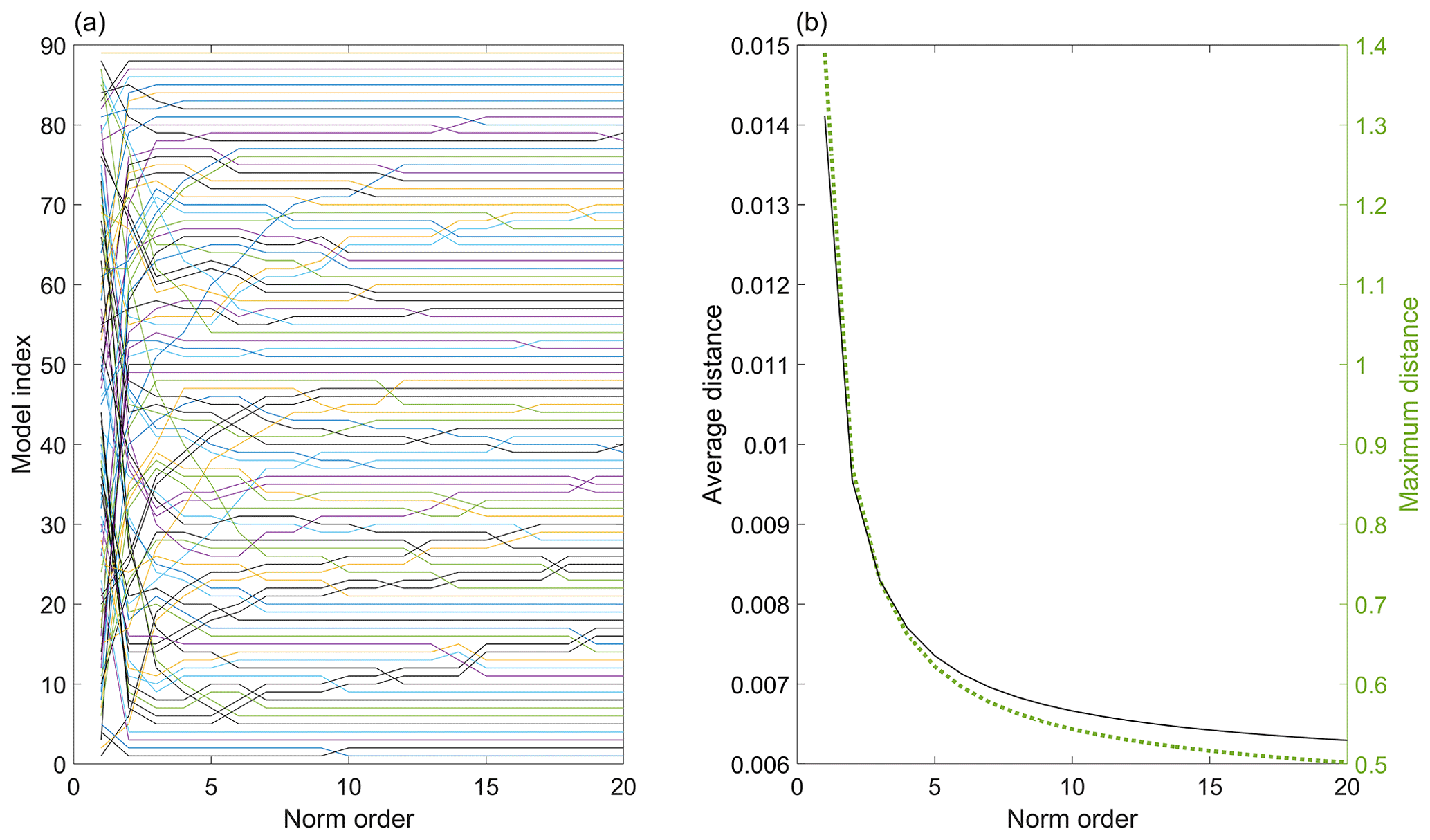
Figure 4 (a) The change in the ranking of the climate models with different norm order (p) and (b) the change in the difference between the maximum and minimum distances and the average distances with different norm order.

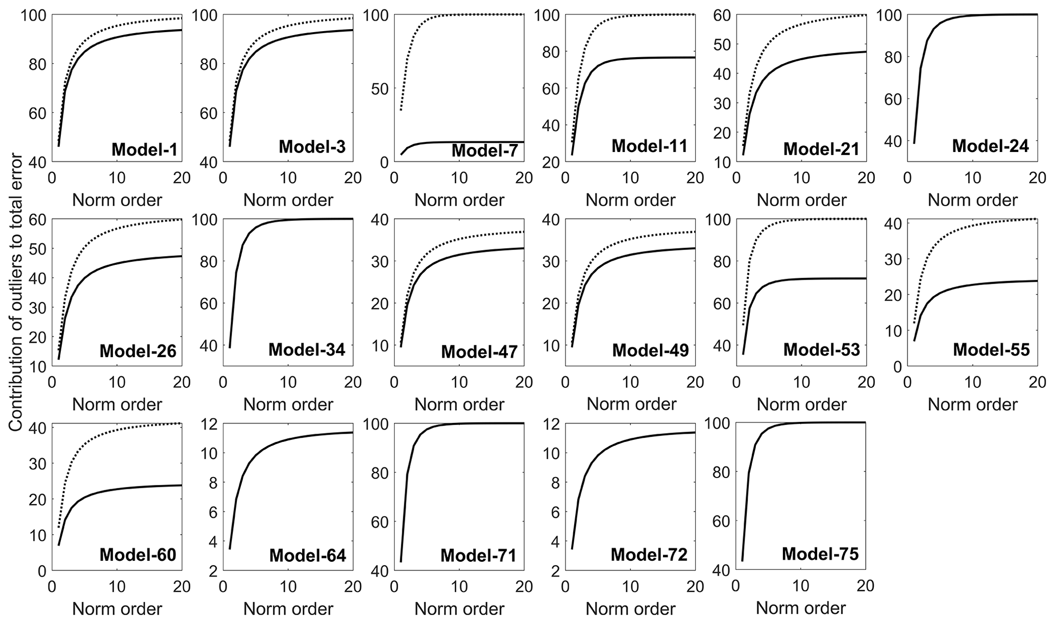
Figure 5 The percentage contribution of outliers to the total error magnitude as a function of norm order. The solid and dotted lines represent different types of outliers.

4 Results

4.1 Regional clustering of error metrics

The study considers 38 error metrics (Table S3) which can take both positive and negative values as input. Similar to the models, the error metrics have been assigned a number (column 1, Table S3), and the error metrics have been labelled as those numbers in some figures.

The clustering technique described in the methodology section can be applied to individual grid points, but for the sake of simplicity, we use a single cluster for all grid points within each of these regions defined by Christensen and Christensen (2007). The methodology is modified slightly to enable regional clustering. At a grid point scale, the maximum value of mean absolute error (u_j) is used as a proxy for that specific error metric at a grid point. For regional clustering, the maximum MAE values are computed for all grid points within the region, and the average of those values is used as a proxy for that region and error metric. This value is then compared with a threshold to determine whether the error metric belongs to a certain cluster or if it should be assigned to a new cluster. The clustering algorithm is executed for multiple thresholds.

The 5th, 10th, and 20th percentiles are selected as potential thresholds to cluster the error metrics. However, users can select any number of thresholds for the sensitivity analysis. The clustering algorithm is allowed to run for all the thresholds to determine the optimal threshold. The efficiency of each cluster for a given threshold is represented by the mean of MAE over all the clusters. Another criterion used to determine the threshold is the number of clusters corresponding to each threshold. An increase in the percentile (q) is expected to increase the MAE as the magnitude of threshold increases. Similarly, the number of clusters are expected to decrease as q increases as it can allow more error metrics into a cluster due to higher threshold magnitude. From Fig. 6, we conclude that the results are according to our expectations. It is found that increasing the percentile resulted in an increase in MAE and a decrease in the number of clusters. The 10th percentile is selected as the threshold to cluster the error metrics for both temperature and precipitation, as it has a smaller number of clusters compared to the 5th percentile and less MAE compared to the 20th percentile.

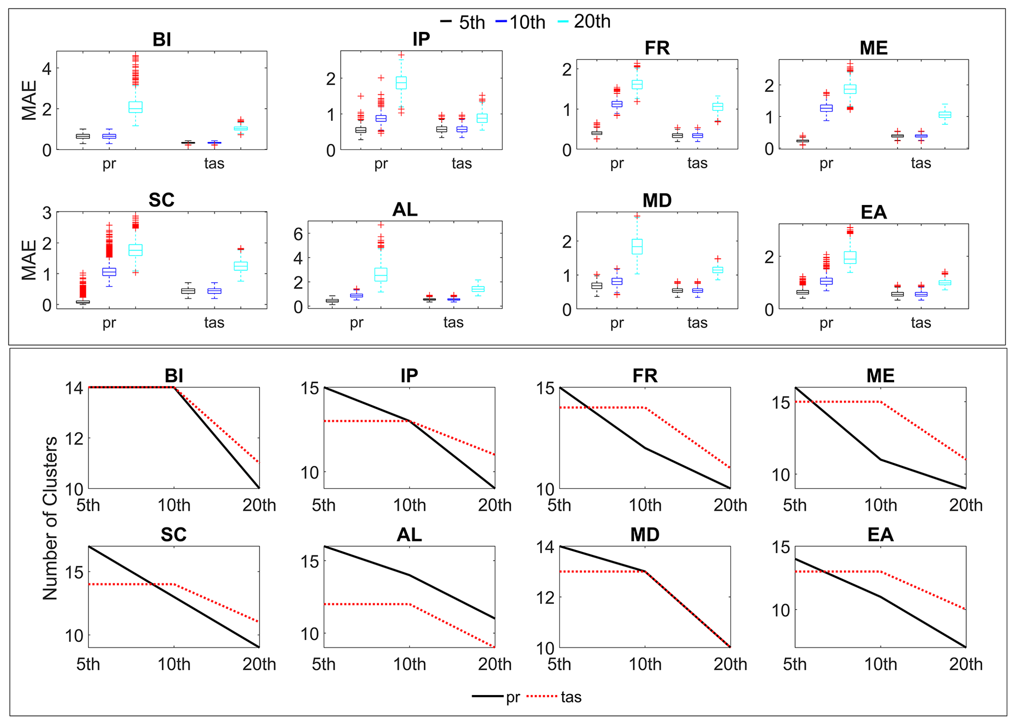
Figure 6 The variation in MAE (first box) and number of clusters (second box) corresponding to the 5th, 10th, and 20th percentiles for precipitation (pr) and temperature (tas) for all the eight regions.

4.2 Results of clustering

4.2.1 Precipitation

For the British Isles region, the classification of 38 error metrics resulted in 15 clusters, with eight error metrics being single-point clusters due to their unique behaviour (Fig. 7). These eight metrics are d [2], (MB) R [17], MdE [19], MEE [21], MV [22], r² [31], SGA [35], and R (Spearman) [36]. The threshold for precipitation data is 6.35, indicating that all eight error metrics produced MAE values greater than 6.35 compared to the remaining 30 error metrics. RMSE [32] and its variants such as normalized RMSE by IQR [25], mean [26], and range [27] are assigned to the same cluster as ED [7], IRMSE [9], MAE [13], MAPD [15], MASE [16], and MSE [23]. The reason could be the L-norm framework which is used by most of the error metrics in this cluster. D1 [3], d1 [4], and d (Mod.) [5], which share a similar framework, are also assigned to a single cluster. Error metrics that evaluate the phase difference between observed and modelled data, including ACC [1], R (Pearson) [30], SC [34], and M [38], are assigned to a single cluster. H10 (MAHE) [8] and MALE [14] share the same cluster as both metrics consider the difference in logarithm of the model and observed data to compute the error. Similarly, MdAE [18] and MdSE [20] are assigned to a single cluster, as both metrics use the median of the difference between observed and modelled data. However, MdE [19] is assigned to a different cluster as it only considers the difference between observed and modelled data without bringing them to the positive domain. NED [24] and SA [33] are found to be in the same cluster, as both metrics are linearly associated while evaluating the model, even though their underlying frameworks are somewhat different. Although ED [7] and NED [24] follow the L2 norm, they are not assigned to the same cluster. This can be attributed to the normalization of observed and modelled data by their respective means in NED, as the statistical parameters such as mean are sensitive to outliers, which can result in changes in ranking order.

Figure 7 Clustering of error metrics using precipitation (pr) data for the British Isles (BI) region. Each error metric can be identified by the number using Table S3.

The Iberian Peninsula region is found to have 17 clusters, with 12 of them being single-point clusters (Fig. 8). Seven of the eight error metrics that are single-point clusters in the British Isles are also single-point clusters in the Iberian Peninsula, except for r² [31]. Five other error metrics – NED [24], KGE (2009) [10], KGE (2012) [11], SA [33], and M [38] – are also single-point clusters in the Iberian Peninsula region. In the British Isles, KGE (2009) [10] and KGE (2012) [11] are assigned to the same cluster. The KGE (2012) is different from KGE (2009) since it used the ratio of coefficient of variation between modelled and observed data instead of the ratio of standard deviation to avoid the cross-correlation between bias and variability ratio. The coefficient of variation is the ratio between the standard deviation and the mean of the data, which represents the extent of variability with respect to the mean of the data. A biased dataset can produce a significant change in the relative standard deviation, i.e. the coefficient of variation. That is a possible reason why both the metrics are in different clusters. r² is assigned to the correlation metrics cluster in this region. The remaining clusters are almost identical to the clusters obtained for the British Isles region.

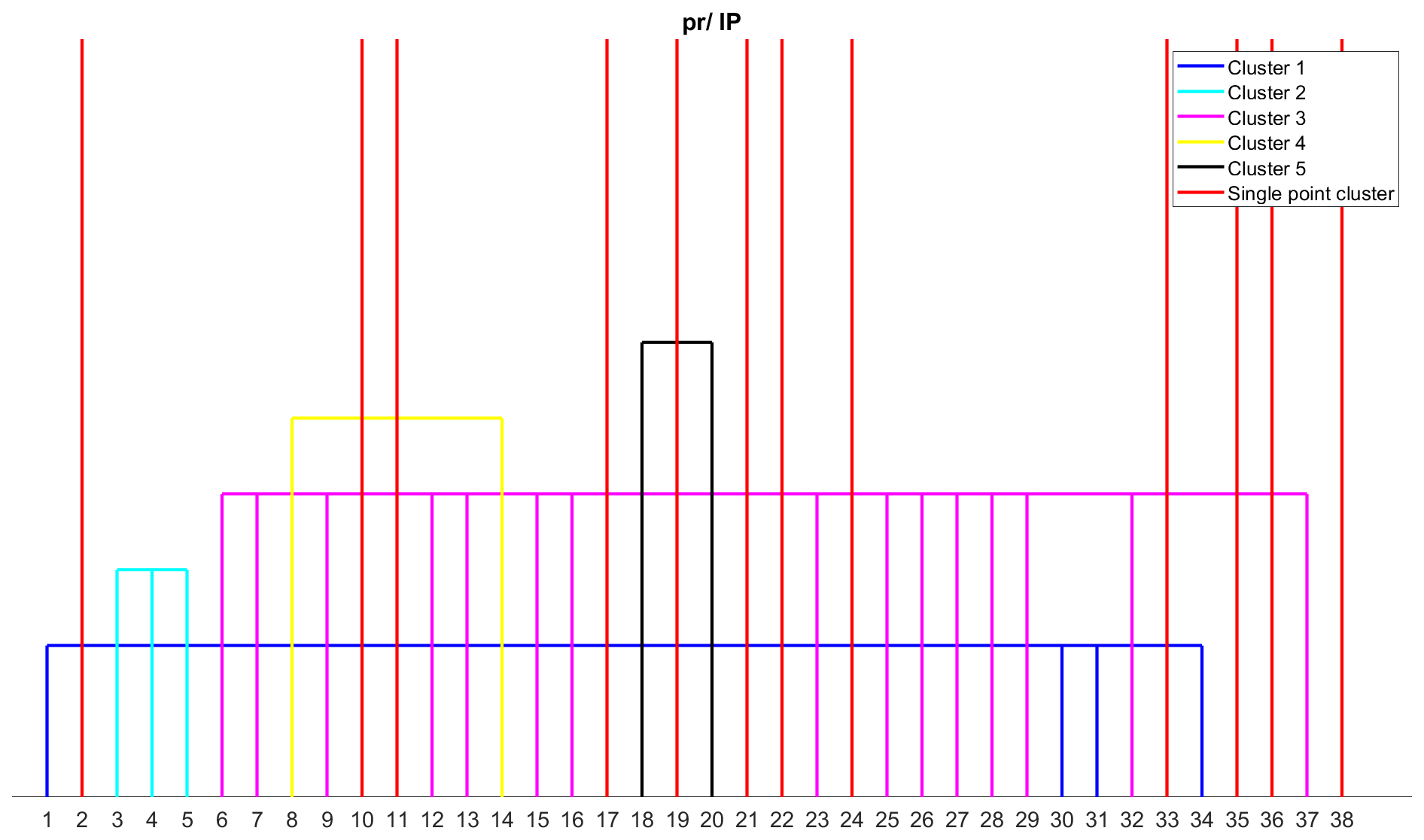
Figure 8 Clustering of error metrics using precipitation (pr) data for the Iberian Peninsula (IP) region. Each error metric can be identified by the number using Table S3.

As the results for the other six regions are similar to either the British Isles or the Iberian Peninsula, we simply summarize their results here and refer the reader to the Supplement for further information. France (Fig. S2), mid-Europe (Fig. S3), Scandinavia (Fig. S4), Alps (Fig. S5), Mediterranean (Fig. S6), and Eastern Europe (Fig. S7) exhibit 15, 15, 16, 16, 17, and 14 clusters, respectively, with 8, 8, 10, 10, 12, and 6 single-point clusters. France and mid-Europe have the same clusters as the British Isles, and the Mediterranean has the same clusters as the Iberian Peninsula. Scandinavia has clusters similar to the British Isles, except that M [38] is a single-point cluster and r² [31] has been assigned to the correlation metrics cluster in Scandinavia. The Alps also have clusters similar to the British Isles, except that KGE (2009) [10] and KGE (2012) [11] are single-point clusters. Eastern Europe also has clusters similar to the British Isles, with the exception that d [2], which is a single-point cluster in the British Isles, forms a new cluster with M [38] in Eastern Europe.

4.2.2 Temperature

Compared to precipitation data, temperature data have a lower number of clusters, which can be attributed to the lower variability in temperature data. The clustering of error metrics for the British Isles is shown in Fig. 9. For the British Isles, 12 clusters are identified, with five single-point clusters, namely KGE (2009) [10], KGE (2012) [11], MV [22], SGA [35], and R (Spearman) [36]. Similar to precipitation clusters, several error metrics, including ED [7], IRMSE [9], MAE [13], MAPD [15], MASE [16], MSE [23], NRMSE (IQR) [25], NRMSE(mean) [26], NRMSE (range) [27], and RMSE [32], are assigned to the same cluster.

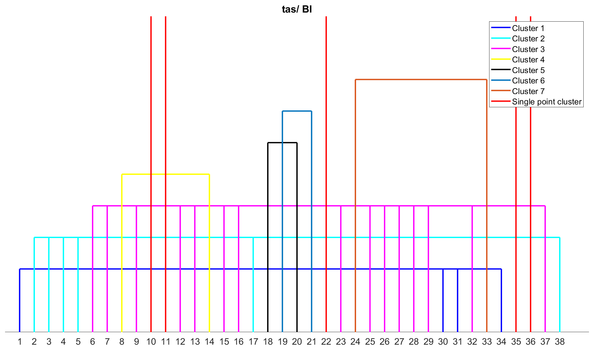
Figure 9 Clustering of error metrics using temperature (tas) data for the British Isles (BI) region. Each error metric can be identified by the number using Table S3.

The correlation metrics, such as ACC [1], r² [31], SCO [34], and R (Pearson) [36], belong to the same cluster. France (Fig. S8) and mid-Europe (Fig. S9) have the same cluster as the British Isles for temperature data. For the Iberian Peninsula (Fig. 10), 13 different clusters are identified, with seven single-point clusters, including MdE [19] and MEE [21] in addition to the five single-point clusters from the British Isles. The remaining clusters are similar to those in the British Isles. Mediterranean (Fig. S10) has the same cluster as the Iberian Peninsula for temperature data, with 13 clusters and seven single-point clusters. Scandinavia (Fig. S11) and Eastern Europe (Fig. S12) have the same number of clusters, i.e. 14 clusters. Scandinavia has eight single-point clusters, whereas Eastern Europe has nine single-point clusters. The Alps (Fig. S13) have 15 clusters, with 10 single-point clusters.

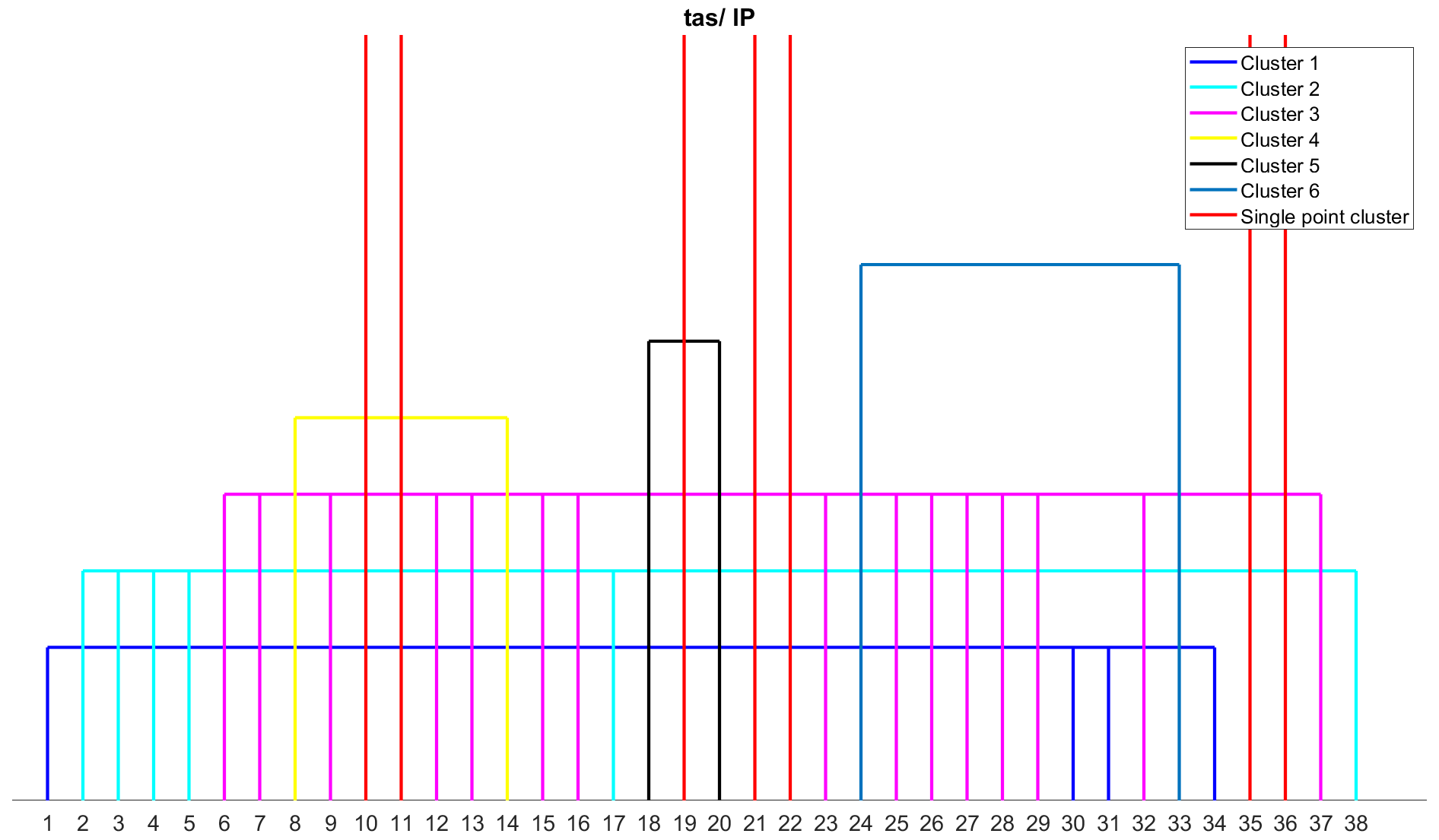
Figure 10 Clustering of error metrics using temperature (tas) data for the Iberian Peninsula (IP) region. Each error metric can be identified by the number using Table S3.

4.3 Bergen metrics

A Bergen metric is computed for all eight regions using the respective clusters for both precipitation and temperature. A single metric is chosen from each cluster randomly; random selection demonstrated no discernible impact on the ranking (see Text S2). Although computed for all 89 regional climate models, this paper focuses on discussing only one climate model for both precipitation and temperature. The Climate Limited-area Modelling (CLM) Community (CLMCom) regional model from the ICHEC-EC-EARTH climate model for r3i1p1 realization is discussed as it performed best at over 25 grid points in five regions and more than two grid points in seven regions. For the temperature variable, the CLMCom model from the CCCma-CanESM2 (Canadian Centre for Climate Modelling and Analysis second generation Canadian Earth System Model) model for r1i1p1 realization is discussed, as it performed best at over 25 grid points in seven regions.

4.3.1 Precipitation

A Bergen metric (BM) is used to assess the performance of the CLMCom model for precipitation in all eight different regions. The BM in the British Isles region is a composite metric that takes into account 15 different error metrics, i.e. ACC, D1, dr, H10 (MAHE), KGE (2009), MdAE, NED, d, MB (R), MdE, MEE, MV, r², SGA, and R (Spearman). Figure 11 provides an overview of the spatial distribution of the BM for all eight regions, while the spatial distribution of each of these metrics is shown in Fig. 12 for the British Isles region.

The magnitude of BM ranges from 0 to 13, with a score of 0 indicating good performance by the model. Based on the results, the CLMCom model performed well in the western part of the British Isles, as indicated by the BM. This is a result of the good performance of most of the individual metrics that comprise the Bergen metric. This is shown in Fig. 12. There are some contradictory results from different error metrics in the eastern region. While all 13 metrics indicate good performance, MV, r², and NED indicate very bad performance by the model.

The use of individual error metrics can provide meaningful insights into the performance of the model in different regions. For example, metrics such as dr, MdAE, MdE, and MEE indicate good performance in the southeastern region, while R (Spearman) indicates bad performance by the CLMCom model, which implies that the phase difference is significant between observed and modelled data in this region. It is worth noting that some metrics, such as r² and R (Spearman), may provide different results even though they share a similar framework. R (Spearman) only tells how well the modelled data follow the observed data, while r² indicates how well the data represent the line of best fit (https://tinyurl.com/y52r3xed, last access: 16 April 2024; https://tinyurl.com/yk2jmsxt, last access: 16 April 2024). Overall, the use of multiple error metrics and the analysis of individual metrics can provide a more comprehensive assessment of the model's performance, particularly in regions where different metrics provide conflicting results.

Figure 11 Spatial distribution of Bergen metric using precipitation data for all the eight regions.

Figure 12 Spatial distribution of the error metrics used to compute the Bergen metric for precipitation and for the British Isles (BI) region. The error metrics have been labelled by the abbreviation, and the corresponding error metrics can be identified from Table S3.

Figure 13 Spatial distribution of the error metrics used to compute the Bergen metric for precipitation and for the Iberian Peninsula (IP) region. The error metrics have been labelled by the abbreviation, and the corresponding error metrics can be identified from Table S3.

Figure 13 shows a Bergen metric for the Iberian Peninsula applied to the CLMCom model, which is based on 17 error metrics obtained from each cluster. These metrics, including ACC, D1, dr, H10 (MAHE), MdAE, d, KGE (2009), KGE (2012), MB (R), MdE, MEE, MV, NED, SA, SGA, R (Spearman), and M, are presented in Fig. 13. The results indicate that the model performs relatively better in the northeast and southeast regions compared to the western region (see Fig. 11), possibly due to the influence of certain metrics such as ACC, R (Spearman), MV, NED, and SA. Additionally, while KGE (2009) and KGE (2012) exhibit similar spatial error patterns, further analysis in the southern region reveals the differences in the magnitude of error. Interestingly, despite their similarity, KGE (2009) and KGE (2012) are classified into different clusters based on a threshold MAE of 5.41 used to determine cluster membership.

France (Fig. S14) and mid-Europe (Fig. S15) have the same clusters as the British Isles, and therefore the same error metrics used in the British Isles are used to calculate the Bergen metric for France and mid-Europe. The Bergen metric indicates an average performance of the model for the entire study region of France (see Fig. 11). While r² shows a very poor performance of the model for France, the MEE metric shows a completely opposite trend, indicating a very good performance of the model. Similar disagreement between r² and MEE is also observed in the British Isles. On the other hand, SGA, which compares the shape of the two signals, shows an average performance by the model. In terms of the spatial distribution of error, the Bergen metric shows lower error magnitudes for MEE in the southeast part of the study region.

The Bergen metric is also used to assess the performance of the CLMCom model for Scandinavia and the Alps using 16 error metrics from each cluster, including ACC, D1, dr, H10 (MAHE), MdAE, NED, d, KGE (2009), KGE (2012), MB (R), MdE, MEE, MV, SGA, R (Spearman), and M. The spatial distribution of these metrics is presented in Fig. S16 (Scandinavia) and Fig. S17 (Alps).

Figures S16 and 11 suggest that the CLMCom model does not perform well for Scandinavia. However, some error metrics, including dr, MdAE, MdE, and MEE, show good performance in the southern part of the region. Although MdAE, MdE, and MEE are assigned to different clusters, they exhibit similar spatial distributions of error. It is worth noting that despite the similarity, the three error metrics are in different clusters due to their higher MAE between them. For the Alps, the Bergen metric indicates a relatively good performance of the CLMCom model. It can be observed in Fig. S17 that all metrics except r² show good performance for the model.

The Mediterranean has the same clusters as the Iberian Peninsula, and the spatial distribution of each metric for the Mediterranean is presented in Fig. S18. The Bergen metric for the CLMCom model suggests an average performance for the entire Mediterranean region. Some of the error metrics, such as KGE (2009), KGE (2012), dr, and MdAE, indicate good model performance. However, metrics such as SGA, SA, and NED show the relatively poor performance of the model.

For Eastern Europe, the Bergen metric is computed using 14 error metrics from each cluster, as listed: ACC, d, D1, dr, H10 (MAHE), KGE (2009), MdAE, NED, MB (R), MdE, MEE, MV, SGA, and R (Spearman). The spatial distribution of each metric is presented in Fig. S19. One notable observation from the figure is the difference between SGA and MEE, which indicates that although the model data have a low bias, the direction of error in the modelled data is completely different from that of the observed data. This insight can be valuable in identifying areas where the model's performance can be improved.

4.3.2 Temperature

For temperature, we focus on the CLM Community (CLMCom) regional model driven by ICHEC-EC-EARTH to demonstrate the application of Bergen metrics for temperature. The spatial distribution of BM is shown in Fig. 14, which indicates average performance by the model, except in certain areas like the northern part of Scandinavia, the central part of Eastern Europe, and the western part of the Iberian Peninsula, where the performance is bad. The British Isles (Fig. 15), France (Fig. S20), and mid-Europe (Fig. S21) regions have 12 clusters, and 12 error metrics, including ACC, d, dr, H10 (MAHE), MdAE, MdE, NED, KGE (2009), KGE (2012), MV, SGA, and R (Spearman), which are used to compute the Bergen metric for these regions.

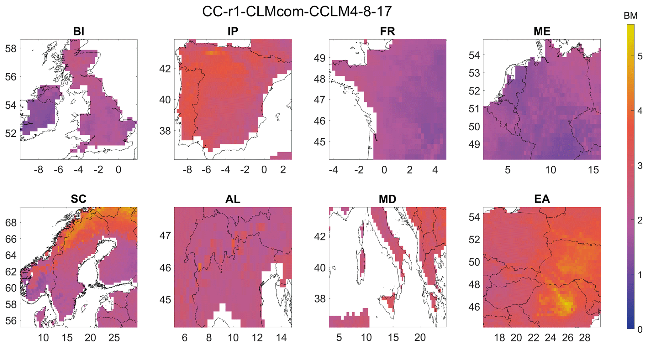
Figure 14 Spatial distribution of Bergen metric using temperature data for all the eight regions.

The Scandinavia (Fig. S22) and Eastern Europe (Fig. S23) regions have 14 clusters, and all the error metrics from the British Isles, along with VE and SA, are used to compute the Bergen metric for these regions. The Iberian Peninsula (Fig. 16) and Mediterranean (Fig. S24) regions each have 13 clusters, and all the error metrics from the British Isles, along with MEE, are used to compute the Bergen metric. The Alps (Fig. S25) region has 15 clusters, with all the error metrics from Scandinavia, including MEE, used to compute the Bergen metric. MdE and MEE consistently indicate very bad model performance for all the regions, while the other metrics indicate relatively good performance. This suggests that the mean and median of the modelled data tend to underestimate/overestimate the observed mean and median, respectively. Histograms in Fig. 17 further investigate this, showing that the error values for ACC are more evenly distributed in the Iberian Peninsula region and close to its ideal point 1, while the source errors for MdE and MEE are concentrated between −0.5 to −1.5, resulting in most of the error values being concentrated between 0.9 and 1 after normalization. The source error represents the distance between the ideal values and actual magnitude after normalization. Similar patterns can be observed in the other regions for temperature.

To illustrate inter-model variability, a random grid point (50.125, 1.875) is selected. The Bergen metric is calculated for both precipitation and temperature at this grid point, and models are ranked based on the Bergen metric (Fig. 18). The Bergen metric ranges from 2.29 to 11.39 for precipitation and 1.85 to 8.37 for temperature. Notably, with a Bergen metric value of 2.29, ETH-COSMO (model 6) is identified as performing well for precipitation. Similarly, with a Bergen metric value of 2.29, GERICS-REMO2015 (model 16) is recognized for its good performance in temperature. The proposed metric offers a valuable tool for assessing the performance of climate models.

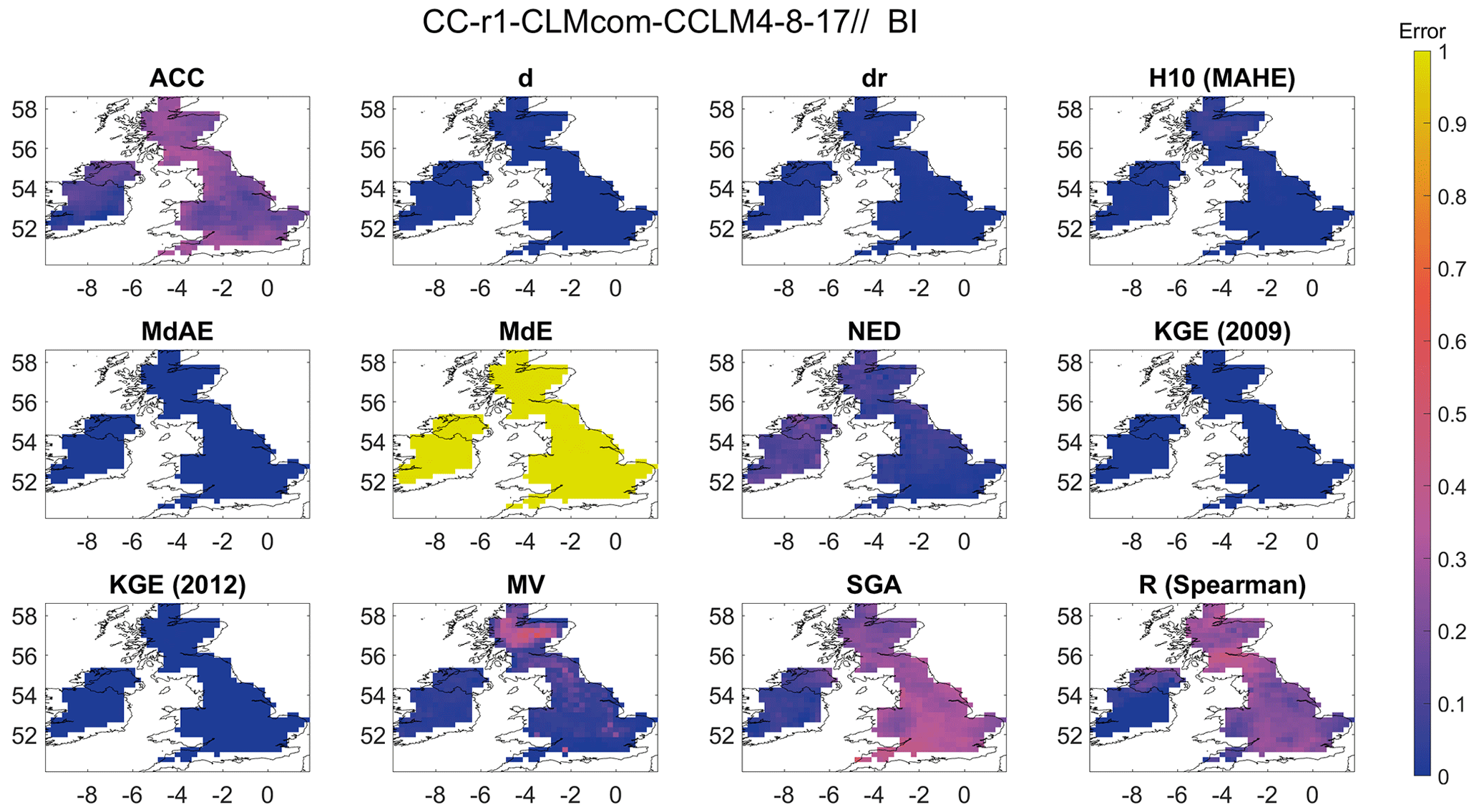
Figure 15 Spatial distribution of the error metrics used to compute the Bergen metric for temperature and for the British Isles (BI) region. The error metrics have been labelled by the abbreviation, and the corresponding error metrics can be identified from Table S3.

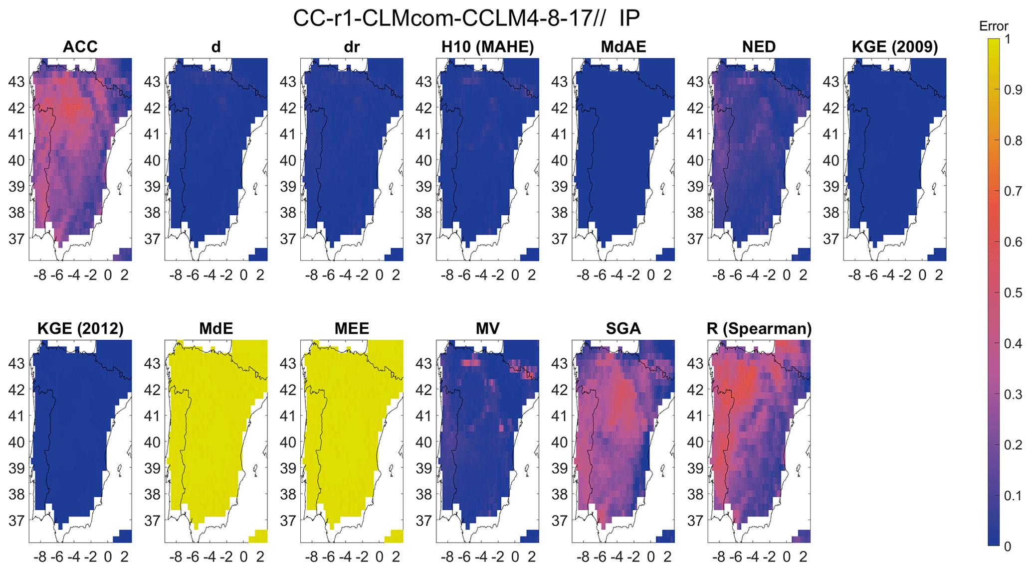
Figure 16 Spatial distribution of the error metrics used to compute the Bergen metric for temperature and for the Iberian Peninsula (IP) region. The error metrics have been labelled by the abbreviation, and the corresponding error metrics can be identified from Table S3.

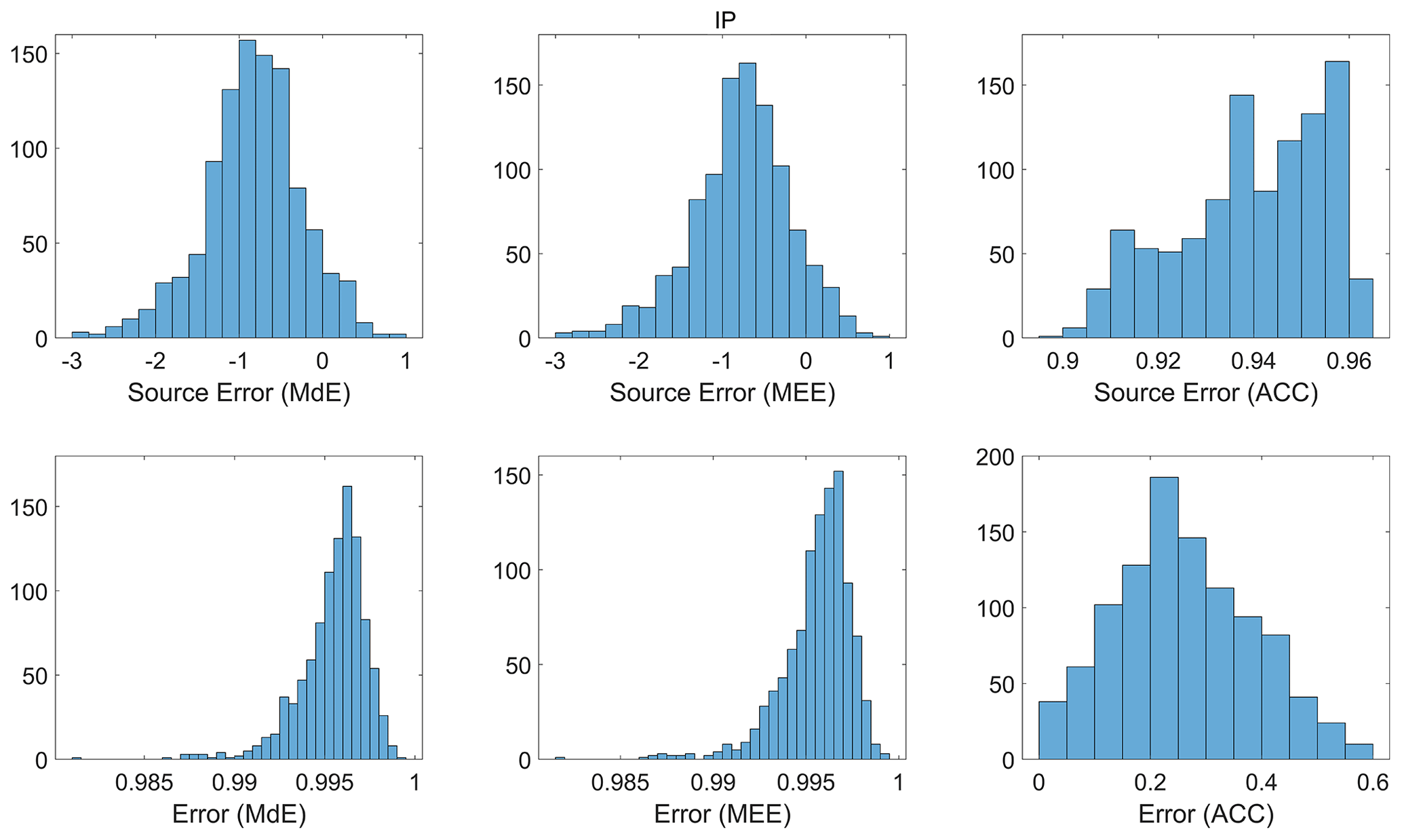
Figure 17 Histogram plot of error and source error for MdE, MEE, and ACC for the Iberian Peninsula region (IP).

Figure 18 The Bergen metric for precipitation (a) and temperature (b) for all 89 climate models, along with the ranking of each model based on the Bergen metric for precipitation (c) and temperature (d) at a grid point (50.125, 1.875).

5 Conclusions

A framework of new error metrics, known as Bergen metrics, has been introduced in this study to evaluate the ability of climate models to simulate the observed climate through comparison with a reference field. The proposed metric integrates several error metrics, as described in the Results section. To generate a single composite index, the methodology uses a generalized p-norm framework to merge all the error metrics. The research determines that the first norm is the most effective norm to use in the analysis.

The study also shows that the number of error metrics used in Bergen metrics can be reduced using a non-parametric clustering technique. Although several clustering techniques are already available in the literature, they come with certain requirements. They require either the number of clusters before running the algorithm or information on the class label of the feature vector. The adopted clustering technique tries to identify the natural cluster present in the data. The mean absolute error based on ranking order is used as a dissimilarity index to assign error metrics to different clusters. The technique also has a threshold parameter: the 5th, 10th, and 20th percentiles are selected as candidates for the threshold parameter, and the 10th percentile of the D matrix is adopted as a threshold in this study. It is selected because an increase in threshold (20th percentile) resulted in an increase in MAE and a decrease in number of clusters, whereas a decrease in threshold (5th percentile) resulted in a decrease in MAE and an increase in the number of clusters; the study chose a middle ground. However, users can investigate different values of q before choosing the threshold. The clustering technique is compared with the k-means clustering approach, and it is found that the non-parametric technique has lower MAE compared to the k-means approach. The clustering is performed for all the eight regions, and those are British Isles, Iberian Peninsula, France, mid-Europe, Scandinavia, Alps, Mediterranean, and Eastern Europe. For precipitation, 15, 17, 15, 15, 16, 15, 17, and 14 clusters are obtained for the eight regions, respectively. For temperature, 12, 13, 12, 12, 14, 15, 13, and 14 clusters are obtained for the eight regions, respectively.

A single error metric from each cluster can be chosen randomly as a component to be used in the calculation of a Bergen metric. We have shown that random selection does not have any effect on the ranking order produced by a Bergen metric. The Bergen metric which uses the L1 framework is found to be less sensitive to outliers compared to the other norms and more stable in higher-dimensional space. Bergen metrics are multivariate error functions that can take any number of error metrics of different variables, as shown in the last section. It can be further modified for a weighting-based metric that can allow the user to give more weightage to particular metrics depending on the requirement of the study. While some metrics show good performance in certain regions, others indicate poor performance. It is also important to observe how a single metric can influence and change the ranking of climate models. Bergen metrics provide a comprehensive evaluation of the model's performance, which is useful for identifying the strengths and weaknesses of the model in different contexts. It is also crucial to underscore that our proposed metric evaluates the magnitude differences between modelled and reference data, prioritizing this aspect over spatial and temporal patterns. The application of this metric should be approached with careful consideration.

Future research should address the sampling uncertainty associated with Bergen metrics. Each data point in time series data has a certain contribution to the total error, and if the contribution is not evenly distributed for all the data points, the metric may give biased results. Also, each metric has probabilistic uncertainty associated with it. For example, RMSE works well when the errors are normally distributed, but what if the errors are not normally distributed? A discussion on uncertainty may yield useful information that will be helpful in removing the bias from climate models in the future.