CLASH – Climate-responsive Land Allocation model with carbon Storage and Harvests

The Climate-responsive Land Allocation model with carbon Storage and Harvests (CLASH) is a global, biophysical land-use model that can be embedded into integrated assessment models (IAMs). CLASH represents vegetation growth, terrestrial carbon stocks, and production from agriculture and forestry for different land uses in a changing climate. Connecting CLASH to an IAM would allow the consideration of terrestrial carbon stocks, agriculture and forestry in global climate policy analyses. All terrestrial ecosystems and their carbon dynamics are comprehensively described at a coarse resolution. Special emphasis is placed on representing the world's forests. Vegetation growth, soil carbon stocks, agricultural yields and natural disturbance frequencies react to changing climatic conditions, emulating the dynamic global vegetation model LPJ-GUESS. Land is divided into 10 biomes with six land-use classes (including forests and agricultural classes). Secondary forests are age structured. The timing of forest harvests affects forest carbon stocks, and, hence, carbon storage per forest area can be increased through forest management. In addition to secondary forests, CLASH also includes primary ecosystems, cropland and pastures. The comprehensive inclusion of all land-use classes and their main functions allows representing the global land-use competition. In this article, we present, calibrate and validate the model; demonstrate its use; and discuss how it can be integrated into IAMs.

1 Introduction

CLASH (Climate-responsive Land Allocation model with carbon Storage and Harvests)¹ is a biophysical land-use model that describes the allocation of land to different uses, forest growth, terrestrial carbon stocks, and the production of agricultural and forestry goods globally. Global land area is divided into 10 biomes, and each biome's area can be allocated to different uses, including agriculture, forestry and primary ecosystems. The biophysical properties of land and vegetation are biome-specific and respond to climate change. The model has been parametrized to emulate the dynamic global vegetation model Lund-Potsdam-Jena General Ecosystem Simulator (LPJ-GUESS) (Smith et al., 2001, 2014; Lindeskog et al., 2021) in varied and changing climatic conditions. In this article, we describe, calibrate, and validate the model and demonstrate its use.

CLASH can be embedded in economic optimization models, and integrated assessment models (IAMs) in particular, or used independently to simulate the climatic impacts of land use in long-term scenarios. However, CLASH has been specifically developed for the former purpose. In this role, CLASH represents the biophysical aspects of land use, while the IAM needs to provide the rationale for why land is used and managed in a specific way, including economic, policy and other societal factors, as well as how the climate changes over time. These factors are relevant for realistic modelling of land use but are outside the scope of CLASH.

Three features make CLASH especially suitable for incorporation into IAMs: (1) its technical design and low computational burden, (2) global geographical coverage, and (3) comprehensive representation of land use and carbon stocks. CLASH is computationally lightweight, is linear, and has an adjustable time step. Many IAMs are written as intertemporal optimization problems (Keppo et al., 2021); i.e., the whole modelling time horizon is considered and solved for optimum within a single optimization problem. Such models can be computationally challenging to solve, especially if the model is nonlinear. CLASH's low computational expense facilitates its incorporation into such IAMs, and given its linear mathematical formulation, it can be incorporated also into IAMs defined as linear programming problems. However, the formulation of the optimization problem is not inherently a part of CLASH but needs to be provided by the IAM. The underlying temporal resolution is annual, which can be flexibly adjusted to match any longer time step, such as 5 or 10 years commonly used in IAMs.

Geographically, CLASH covers all global land area and depicts the global production of goods in agriculture and forestry. The model covers the carbon stocks of vegetation, litter, and soil and describes how they are affected by land use and climate change. The effects of climate change on vegetation growth and soil carbon dynamics are modelled as a function of global mean temperature change and atmospheric CO₂ concentration, as these two variables are standard outputs of many IAMs. Together, the global coverage, representation of main terrestrial carbon stocks and the inclusion of climate change effects on terrestrial ecosystems make CLASH suited for examining land-based climate change mitigation and adaptation measures at the global scale and over long time horizons.

Embedding CLASH in an IAM enables the optimization of land-use and forest management over a multi-decadal time frame in a changing climate and the representation of the optimal contribution of the land-use sector towards the global climate change mitigation effort. This capability fills a critical, vacant niche in the model ecosystem. Towards this role, CLASH combines some features from three model types.

1. Dynamic global vegetation models (DGVMs), such as LPJ-GUESS (Smith et al., 2001, 2014; Lindeskog et al., 2021), can be used to depict how vegetation responds to changing climatic conditions. DGVMs are notably more detailed than CLASH. In DGVMs, however, land use can only be depicted by exogenous scenarios. It cannot be optimized. Due to their high level of detail and heavy computational burden, DGVMs cannot be embedded in IAMs in the way that CLASH can.

2. Economic partial equilibrium models of the land-use sector, such as MAgPIE (Dietrich et al., 2019) and GLOBIOM (Havlík et al., 2018), enable the optimization of land use within a time step, while recursive-dynamics rules represent the evolution over years. Such models represent land use comprehensively and can be linked to IAMs (Fricko et al., 2017). However, as they stem from an agricultural economic modelling tradition, the models do not necessarily represent comprehensively the dynamic changes in the age structure of forests (GLOBIOM) or allow for intertemporal optimization (MAgPIE and GLOBIOM). Both features are needed to enable the full dynamic optimization of forest structure and management over long time horizons, e.g. when aiming for long-term climatic targets.²

3. Forest sector models, such as the GTM (Sohngen et al., 1999), include the forest age structure and rely on intertemporal optimization as the solution concept. Although forest sector models have been linked to IAMs (Sohngen and Mendelsohn, 2003; Tavoni et al., 2007; Favero and Mendelsohn, 2014) and explicit, age-structured representations of forests have been built into IAMs (Siljander and Ekholm, 2018), they do not depict land use comprehensively as they (by definition) focus on the forest sector.

In particular, CLASH covers the climate-responsive vegetation growth and the representation of vegetation and soil carbon stocks from DGVMs, crop and livestock production from land-use models, age-structured forests and harvesting of wood from forest sectors models, and the possibility for optimizing land use from both types of partial equilibrium models. What is left out is the product demand, markets and policies that drive land-use decisions in partial equilibrium models, and the detailed biophysical modelling of ecosystems in DGVMs. Also, agriculture and forest management are described in less detail and without detailed management options than in models focusing on each aspect individually.

This paper provides a proof-of-concept description for the model and how it could be utilized. The current parametrizations of CLASH are based on non-bias-corrected climate data, which can lead to some deviation from reality regarding vegetation characteristics. New parametrizations based on bias-corrected data will be provided with subsequent model versions and should be used for analyses.

The rest of the article is organized as follows. In Sect. 2, we describe the structure of the model and the modelling of vegetation, soils, and crop and timber yields. In Sect. 3, we present the calibration of the model, and in Sect. 4, we present the validation of this calibration against the global terrestrial carbon stocks projected by LPJ-GUESS. As a demonstration of the model, we analyse in Sect. 5 how different demand scenarios for agricultural and forestry products affect the possibilities for enhancing terrestrial carbon stocks. Last, in Sect. 6, we further discuss the integration of CLASH with IAMs and the possible uses the model might have.

2 Model structure

2.1 Dimensions and variables

The basic dimensions of CLASH are biomes b∈B into which global land area is divided, land-use categories u∈U, and time steps t∈T. The basic time step resolution is annual, but most use cases – especially when combined with an IAM – require using a multi-year time step, such as 10 years. The age structure of secondary forests is modelled though age classes a∈A.

The variables describe

• land area (by biome, land-use type and time step),

• carbon stocks in vegetation (by biome, land-use type and time step),

• carbon stocks in woody and herbaceous litter and soil (by biome and time step),

• areas of forest clearing (by biome, age class and time step),

• harvested crops and wood (by biome and time step),

• headcount and product yield of agricultural animals (by time step), and

• CH₄ and N₂O emissions from agriculture (by biome and time step).

2.2 Ecological and land-use modules

CLASH consists of a land-use module and an ecological module. The land-use module contains the variables and equations for land allocation, terrestrial carbon stocks, and harvesting, and it is the part that can be integrated into an IAM. The ecological module is used to calibrate the land-use module's parameters based on the trajectories of climate change. The ecological module is not designed to be integrated into the IAM, as it would violate the linear formulation required by many IAMs.

Climate change affects vegetation growth through changes in local factors, such as temperature and precipitation. In CLASH, vegetation growth and other ecological processes emulate results from LPJ-GUESS, which is run on a spatial grid in different climate scenarios and thus accounts for the regional differences in growing conditions in current and future climates. The biomes in CLASH are large and cover somewhat heterogeneous conditions and responses to climate change (e.g., some parts of a tropical biome may become drier, while others get wetter). The CLASH parametrizations thus depict the average conditions within each biome. To account for climate change, the parametrizations are done as a function of global mean temperature and carbon dioxide concentration, standard outputs of many IAMs. These serve as proxies for the changes on local climatic factors, which are nevertheless modelled explicitly in LPJ-GUESS.

The division into two separate modules was done to satisfy two conflicting model design requirements: (1) the land-use module must be linear and computationally lightweight and (2) ecological conditions must respond to climate change. Some ecological parameters depend nonlinearly on climatic conditions, but including this climate dependence in the land-use module would make the model nonlinear and involve more complex calculations. Instead, linearity is maintained in the land-use module through fixed, time-varying parameter values to depict vegetation growth, disturbances, yields and carbon dynamics, which change over time according to a predetermined climate change scenario. When CLASH is integrated into and IAM, one can iteratively run the IAM and then re-calibrate the parameters with the ecological module, using the climate trajectory in the IAM's solution. The procedure is repeated until consecutive solutions converge, and the ecological parameter values align with the climate trajectory. Whether the iterative procedure is necessary depends on the IAM and scenario design.

2.3 Land area allocation

Global land area is divided into 10 biomes based on the USDA major biomes classification (Reich and Eswaran, 2020). Biomes of marginal importance to agriculture, forestry and carbon stocks – such as ice and permafrost – are aggregated into a single unproductive class. We keep the geographical boundaries of biomes constant over time, even as the climate changes. Instead, the ecological parameters depicting vegetation growth, disturbances, agricultural yields and carbon dynamics respond to climate change. A map of the applied biome classification is presented in Fig. 1.

Two requirements guided the choice of classification: conciseness (i.e., having only a relatively small number of biomes) and relative homogeneity (i.e., keeping the variation in growth and carbon dynamics within each biome small). These are conflicting requirements, as greater conciseness leads to less homogenous biomes. The USDA major biomes classification was chosen as the basis for the biomes in CLASH, as it divides the world to relatively few biomes, but which were more homogenous than with alternative classifications, such as the Köppen–Geiger climate classification or Holdridge life zones.

The land-use classes in CLASH are based on the Land-Use Harmonization dataset (LUH2) (Hurtt et al., 2020). The classes are cropland, pasture (including rangeland), primary ecosystems (including primary forest and primary non-forest), secondary forest, secondary non-forest and urban land. Primary ecosystems are ecosystems that have not been notably altered by direct human disturbance. Secondary forests have been logged at least once or have been established on previously unforested land. Secondary non-forest is land that is not actively used but has been subject to human land use. Land cannot be converted back into primary ecosystems. Hence, once cleared, primary ecosystems cannot be regained.

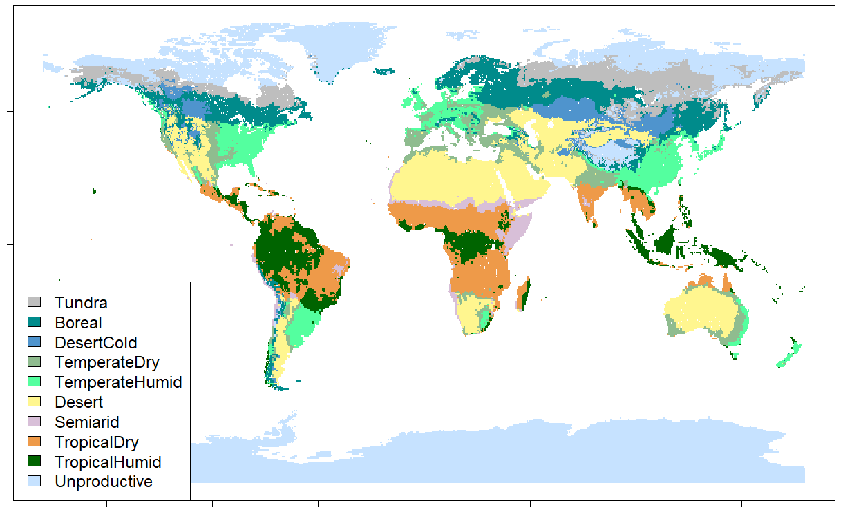
Figure 1 Biome classification used in the CLASH model.

The land-use module allocates land area to different uses, which affects the production quantities of goods (food and feed crops, wood, etc.) and carbon storage in vegetation and soil. Land use in each biome, b, is constrained by the biome's total land area A_b (million km²). This area is distributed between land uses, u, and the area of land use u in period t is $A_{b,u,t}$. Hence, for all biomes b and time steps t,

$$\begin{array}{}\text{(1)}& {\sum }_u{A}_{b,u,t}=A_b.\end{array}$$

Secondary forests (u=secdf) are further divided into age classes. The width of each age class is the same as the model time step (e.g. 10 years). All secondary forest area, $A_{b,\mathrm{secdf},t}$, must belong to one age class, ${\widehat{A}}_{b,\mathrm{secdf},t,a}$. Hence,

$$\begin{array}{}\text{(2)}& {\sum }_a{\widehat{A}}_{b,\mathrm{secdf},t,a}=A_{b,\mathrm{secdf},t}.\end{array}$$

Between time periods, secondary forests can age, be harvested or get destroyed by disturbance events like forest fires. Ageing forest land area will shift to the next age class in the following time period. Area cleared by harvests or destroyed by forest disturbances is allocated to the youngest age class in the next period if replanted, or it is converted into other land use and thereby subtracted from the secondary forest area. Other land converted to secondary forest is added to the youngest age class.

2.4 Vegetation carbon stocks

Vegetation carbon stocks (GtC) are calculated by multiplying land area $A_{b,u,t}$ (million km²) by vegetation carbon density $d_{b,u,t}$ (kgC m⁻²). Vegetation carbon densities for all land uses across biomes are projected by the ecological module based on global mean temperature and atmospheric CO₂ concentration scenarios provided to the module.

Vegetation on cropland and pastures is short-lived compared to the model time step and hence assumed to regenerate within each model period. Cropland vegetation is represented by an aggregate crop that reflects the weighted-average properties of all crops cultivated in the biome. Likewise, pasture vegetation is depicted by representative grasses. As the vegetation regenerates frequently, the amount of vegetation and its carbon density in period t is solely determined by current growth conditions (i.e., not on pre-existing vegetation stock or past growth conditions). The growth conditions in biome b depend on the global mean temperature, T_t, and the atmospheric CO₂ concentration, C_t.³ The dependence is characterized by the function

$$\begin{array}{}\text{(3)}& d_{b,u,t}={\mathit{\alpha }}_{b,u}+{\mathit{\beta }}_{b,u}{T}_t+{\mathit{\gamma }}_{b,u}{C}_t,\end{array}$$

where α_b,u, β_b,u and γ_b,u are parameters estimated by fitting the function to data from LPJ-GUESS simulations.

Similarly, the growth of secondary forests reflects the average properties of forests in each biome. Unlike vegetation on cropland and pasture, trees are long-lived and the carbon density depends on the stand age and the climatic conditions the trees have grown in. Relatedly, forest growth depends on the growth conditions characterized by the current climate and the stand's current state (characterized by the growth history and thus the past climate).

For a stand currently in age class a, the next-period carbon density $d_{b,\mathrm{secdf},t+\mathrm{1},a+\mathrm{1}}$ depends on its current density $d_{b,\mathrm{secdf},t,a}$ and the relative growth rate, $g_{b,\mathrm{secdf},t,a}$:

$$\begin{array}{}\text{(4)}& d_{b,\mathrm{secdf},t+\mathrm{1},a+\mathrm{1}}=d_{b,\mathrm{secdf},t,a}(\mathrm{1}+g_{b,\mathrm{secdf},t,a}),\end{array}$$

where

$$\begin{array}{}\text{(5)}& \begin{array}{rl}{g}_{b,\mathrm{secdf},t,a}& =d_{b,\mathrm{secdf},t,a}^{{\mathit{\delta }}_b+{\mathit{\epsilon }}_b{d}_{b,\mathrm{secdf},t,a}}\\ & \left({\mathit{\eta }}_b+{\mathit{\theta }}_b{T}_t+{\mathit{\kappa }}_b{C}_t+\left({\mathit{\lambda }}_b+{\mathit{\mu }}_b{C}_t\right)T_t^{\mathrm{2}}\right).\end{array}\end{array}$$

Parameters δ_b, ε_b, η_b, θ_b, κ_b, λ_b and μ_b are estimated from LPJ-GUESS simulations of forest growth in various scenarios of changing climate (see Sect. 3).

Primary ecosystems encompass primary forest and primary non-forest. Their vegetation is long-lived. However, unlike in the case of secondary forests, the age structure (and, hence, the growth and disturbance dynamics) of primary ecosystems need not be modelled explicitly.⁴ The carbon density of primary ecosystems, $d_{b,\mathrm{primary},t}$, is a landscape-level average that accounts implicitly for the age structure and the growth conditions of primary ecosystems. Its dependence on climatic conditions is characterized by the function of the same form as in Eq. (3).⁵

Secondary non-forest is a small but diverse category of land. It contains areas that are recovering from human influence, including, for example, deforested land that is not claimed for another use and abandoned croplands and pastures. Hence, the carbon density of secondary non-forest varies notably depending on local climatic conditions, earlier land use, and the degree and time since the human influence on them. These factors make the modelling of the associated vegetation and carbon stock very difficult. As the composition of vegetation on secondary non-forest land is not specified in the LUH2 dataset, we assume due to lack of data that vegetation is growing naturally in these areas. This possibly overestimates the amount of biomass and stored carbon to some degree.

Urban areas cover currently only 0.4 % of the global land area (Hurtt et al., 2020). As vegetation carbon stocks in urban areas are insignificant compared to the global total, they are omitted from CLASH. As urban areas do not contribute to carbon storage or producing agricultural and forestry products in CLASH, the urban area needs to be fixed to an exogenous scenario in a typical use case of the model.

2.5 Litter and soil carbon stocks

Litter and soil carbon stocks (measured in GtC) are modelled through dynamic stock equations that account for their accumulation, decay into atmosphere and transfer of carbon from the litter to the soil stock. Each biome b has separate litter and soil carbon stocks for woody and herbaceous matter, $L_{b,k,t}$ and $S_{b,k,t}$, distinguished by the subindex $k\in \left\{\mathrm{woody},\mathrm{herb}\right\}$. This distinction allows accounting for differences in their decay. The woody matter accumulates from primary ecosystems, secondary forests and secondary non-forests, as well as herbaceous matter from croplands and pastures. As these stocks are not directly linked to the land area under each land-use category, land-use change does not affect existing stocks but only the accumulation of carbon.⁶

Vegetation generates litter. Its amount is defined as the difference between the annual net primary production (NPP) and the annual change in the vegetation carbon density. Additionally, in forests, harvests produce logging residues that increase the influx of woody litter, and on cropland, harvests remove a part of the carbon fixed by NPP, reducing the litter carbon influx. The total annual litter carbon influx is denoted by I_bkt.

The fraction $\left({\mathit{\nu }}_{b,k}+{\mathit{\xi }}_{b,k}{T}_t\right)$ of the litter stock decays into the atmosphere annually. Here, ν_b,k is the base decay rate for biome b and ξ_b,k T_t represents the effect of climate change on the litter decay. A fraction ρ_b,k of litter carbon is transferred to the soil carbon stock. Carbon that is not released into the atmosphere or transferred into soil remains in litter. Analogously, the fraction ${\mathit{\sigma }}_{b,k}+{\mathit{\tau }}_{b,k}{T}_t$ of soil carbon decays annually to the atmosphere. This leads to the dynamic equations for litter and soil carbon stocks:

$$\begin{array}{}\text{(6)}& \begin{array}{rl}{L}_{b,k,t+\mathrm{1}}& =L_{b,k,t}\left(\mathrm{1}-{\mathit{\nu }}_{b,k}-{\mathit{\xi }}_{b,k}{T}_t-{\mathit{\rho }}_{b,k}\right)+I_{b,k,t}\\ S_{b,k,t+\mathrm{1}}& =S_{b,k,t}\left(\mathrm{1}-{\mathit{\sigma }}_{b,k}-{\mathit{\tau }}_{b,k}{T}_t\right)+{\mathit{\rho }}_{b,k}{L}_{b,k,t}.\end{array}\end{array}$$

2.6 Forest disturbances

Forest fires are the only natural disturbance in CLASH at the moment. Fires are modelled as stand-replacing disturbances. A certain share of secondary forest area in each age class burns every year, and this average fire probability changes over time with the climate. Fires also affect primary ecosystems, but the effect is not explicitly modelled: the disturbance regime and climate-induced changes are implicitly accounted for in the carbon density of primary ecosystems.

The fire probability was modelled to depend on the global mean temperature (which drives changes in local temperature and precipitation) and the CO₂ concentration (CO₂ fertilization affects forest growth, which affects fire probability through fuel load). The linear relationship between fire probability and the climate variables is equivalent to Eq. (3), and the parameters of this equation were estimated from LPJ-GUESS simulations for natural forests.

2.7 Crop and wood harvests

Food, feed and energy crops are harvested from cropland. Each biome's average crop yield y_b,t (kgDM m⁻² yr⁻¹) is a weighted average of the yields of the five plant functional types (PFTs) grown on cropland (C3 annuals, C4 annuals, C3 perennials, C4 perennials and C3 nitrogen fixing plants) and accounting for the share of irrigated and rainfed crops at each location. We used LPJ-GUESS defaults for irrigation, fertilization and other cropland management options (Lindeskog et al., 2013; Olin et al., 2015). We assumed externally an average 80 % cropping intensity (Siebert et al., 2010), as our LPJ-GUESS simulation protocol did not account for this. The average crop yield is represented by the same functional form as was used with vegetation carbon density, in Eq. (3). Total crop harvest in each biome is the product of average crop yield and cropland area.

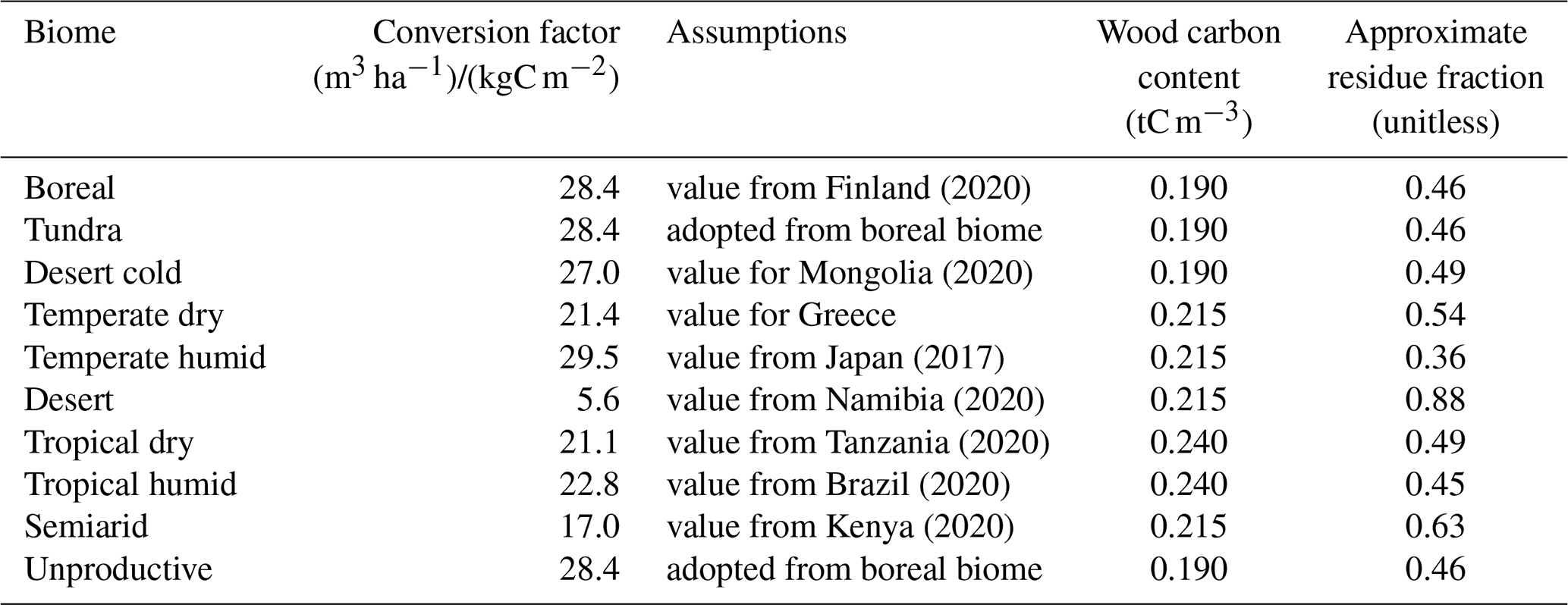
Wood is harvested from secondary forests and cleared primary ecosystems by clear-cutting. Wood harvests depend on harvested area and the stocking density (i.e. stem volume) $v_{b,u,t,a}$ (m³ ha⁻¹) of the harvested forests, which varies across biomes, as well as across age classes for secondary forest. The stem volume is calculated by multiplying the carbon density, $d_{b,u,t,a}$ (kgC m⁻²) with the conversion factor, γ_b ((m³ ha⁻¹)/(kgC m⁻²)), which accounts for the conversion from carbon mass to dry biomass and from dry biomass to stem volume. Hence,

$$\begin{array}{}\text{(7)}& v_{b,u,t,a}={\mathit{\gamma }}_b{d}_{b,u,t,a}.\end{array}$$

The conversion factors applied in CLASH are based on data from FAO's Global Forest Resources Assessment 2020 country reports (FAO, 2023). Their values are displayed in Table 1.⁷

Wood harvesting generates three timber grades: logs, pulpwood, and energy wood (m³ yr⁻¹) and forest residues (kgDM yr⁻¹), which includes all biomass not covered by the aforementioned categories. The largest parts of large stems qualify as logs and may be used for timber. Pulpwood includes small stems, thin parts of large stems and large branches. Energy wood are treetops, very small stems and small branches. Residues may be harvested or left on-site, in which case the carbon in them enters the woody litter carbon pool.

Table 1 Conversion factors for translating vegetation carbon density (kg m⁻²) into stem volume (m³ ha⁻¹).

The division of stem volume into timber grades depends on the stem volume $v_{b,u,t,a}$. Stands with very small trees and low stocking density provide only energy wood; stands with large trees and high stocking density provide mostly logs and some pulpwood.⁸ Let ${\mathit{\sigma }}_i\left(v_{b,u,t,a}\right)$, where $i\in \left\{\mathrm{energy},\mathrm{pulp},\mathrm{logs}\right\}$, denote the share of each timber grade as a function of stocking density. We assume the following breakdown:

$$\begin{array}{}\text{(8)}& {\mathit{\sigma }}_{\mathrm{energy}}=\left\{\begin{array}{ll}\mathrm{1}& \mathrm{when}{v}_{b,u,t,a}<\mathrm{20}\\ \mathrm{1}-\mathrm{0.0085}& \mathrm{when}\mathrm{20}\le v_{b,u,t,a}\\ \left(v_{b,u,t,a}-\mathrm{20}\right)& \le \mathrm{120},\\ \mathrm{0.15},& \mathrm{when}\mathrm{120}<v_{b,u,t,a},\end{array}\right.\end{array}$$

and

$$\begin{array}{}\text{(9)}& {\mathit{\sigma }}_{\mathrm{logs}}=\left\{\begin{array}{ll}\mathrm{0}& \mathrm{when}{v}_{b,u,t,a}<\mathrm{80},\\ \left(\mathrm{1}-{\mathit{\sigma }}_{\mathrm{energy}}\right)& \mathrm{when}\mathrm{80}\le v_{b,u,t,a}\\ \mathrm{0.00425}{v}_{b,u,t,a}& \le \mathrm{280},\\ \left(\mathrm{1}-{\mathit{\sigma }}_{\mathrm{energy}}\right)\mathrm{0.85},& \mathrm{when}\mathrm{280}<v_{b,u,t,a},\end{array}\right.\end{array}$$

and

$$\begin{array}{}\text{(10)}& {\mathit{\sigma }}_{\mathrm{pulp}}=\mathrm{1}-{\mathit{\sigma }}_{\mathrm{energy}}-{\mathit{\sigma }}_{\mathrm{logs}}.\end{array}$$

Let ϑ_b and ρ_b denote respectively the carbon density of wood in biome b (Table 1)⁹, and the fraction of total biomass carbon is contained in residues. As residues contain all carbon not contained in the stems, we define

$$\begin{array}{}\text{(11)}& {\mathit{\rho }}_b:={\displaystyle \frac{d_{b,u,t,a}-{\mathrm{10}}^{-\mathrm{1}}{\mathit{\vartheta }}_b{v}_{b,u,t,a}}{d_{b,u,t,a}}}=\mathrm{1}-{\displaystyle \frac{{\mathit{\vartheta }}_b{\mathit{\gamma }}_b}{\mathrm{10}}}.\end{array}$$

2.8 Livestock

CLASH includes a representation of livestock to account for the land area needed for cattle grazing and cultivating livestock feed crops, as well as for the CH₄ and N₂O emissions from livestock management. We consider four kinds of livestock that only produce meat – beef cattle, pigs, broiler chicken and “shoats” (aggregated sheep and goats) – as well as dairy cattle that produces milk and beef and laying hens that produce eggs. The livestock variables covered in the model are headcount per animal type (millions), production of each animal product (Mt yr⁻¹), and CH₄ and N₂O emissions from enteric fermentation and manure management (Mt yr⁻¹).

Table 2 displays the animal products' modelling assumptions for global current herd size and per-head pasture and feed requirements (for modelling the land use for animal husbandry), product yields (for modelling the supply of animal products), GHG emissions factors (for modelling the animals' climatic impacts) and average-animal characteristics (provided for reference).

Table 2 Data and assumptions used in the livestock module.

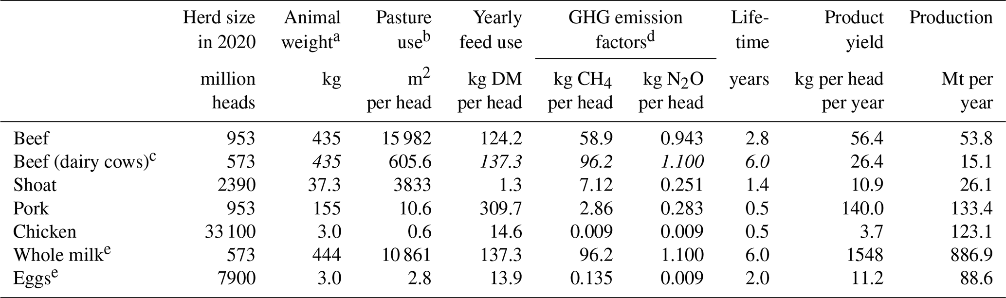
^a Liveweight. ^b Total global in-use pasture area assumed to be 2.1 billion hectares (Mottet et al., 2017; Poore and Nemecek, 2018). ^c Beef from culled dairy cows; shared values across the two sub-systems are repeated and printed in italic. ^d Emissions from manure management and, for ruminants, enteric fermentation. ^e Demand and product yield refer to the product (milk or eggs) and the rest to the product-delivering animal (dairy cow or laying hen).

The annual product yields of cow milk and chicken eggs per head (i.e., per producing animal) were obtained from FAO (2023). Similar (albeit theoretical) annual product yields of meat per head were calculated for meat-producing animals as follows. First, the boneless meat yield per animal was estimated by multiplying its average liveweight (cattle: Dong et al., 2006; others: Gavrilova et al., 2019) by the share of boneless meat of the animal's mass (Knight and Rentfrow, 2020; Wilfong and O'Quinn, 2018). Second, the average slaughter age was approximated based on the size of the global herd and the number of animals slaughtered annually (FAO, 2023). Finally, the annual product yield of meat per head was calculated by dividing the boneless meat yield by the average slaughter age.

The livestock carbon stock is insignificant, around 0.1 Gt C (Bar-On et al., 2018), and is therefore omitted from the model. The emission factors for methane and nitrous oxide were obtained respectively from Gavrilova et al. (2019) and Jun et al. (2000). Pasture use was obtained from Mottet et al. (2017) and Poore and Nemecek (2018). A biome-specific pasture use per animal was calculated from this global average by using the NPP of pastures in each biome, so that the biome-specific pasture use weighted with the pasture area in year 2020 matches the global average pasture use per animal, as presented in Table 2. Yearly feed use per head was obtained from Mottet et al. (2017).¹⁰ The crops consumed as animal feed are produced on cropland, which implies that livestock also requires cropland to produce the necessary feed.

3 Data and model fitting

3.1 LPJ-GUESS

To estimate the parameters of CLASH that define growth, disturbances, yields and carbon dynamics in each biome, we used data generated by the LPJ-GUESS model (Smith et al., 2001, 2014; Lindeskog et al., 2021) run globally with a 2°×2° grid in different climatic scenarios. LPJ-GUESS is a second-generation dynamic global vegetation model (DGVM) which has been optimized for regional to global applications. It includes a detailed representation of forest ecosystem composition and stand dynamics. It can simulate, for example, vegetation growth and succession (Smith et al., 2014) and vegetation shifts under future climate scenarios (Hickler et al., 2012). A detailed description of LPJ-GUESS is available in Smith et al. (2001). We used LPJ-GUESS version 4.0 with global PFTs.

The model simulates potential vegetation as a mixture of 19 PFTs which compete with each other for light, space and soil resources in each simulated grid cell. Each PFT is characterized by growth form, phenology, photosynthetic pathway (C₃ or C₄), bioclimatic limits for establishment and survival. Additionally, woody PFTs are characterized by allometry. In “cohort mode”, all individuals of a given age cohort are assumed identical (Knorr et al., 2016). The ecosystem processes are updated daily but carbon allocation is only updated annually. Crop sowing and harvesting dates are determined dynamically based on local climatology (Lindeskog et al., 2013).

Biomass-destroying disturbances are turned off, but wildfire probability is modelled prognostically based on weather, fuel continuity (litter) and human population density using the SIMFIRE-BLAZE model where the simple global fire model (SIMFIRE) calculates total burned area (Knorr et al., 2014) with total fire carbon flux calculated from BLAZE (BLAZe-induced land-biosphere-atmosphere flux Estimator) (Rabin et al., 2017).

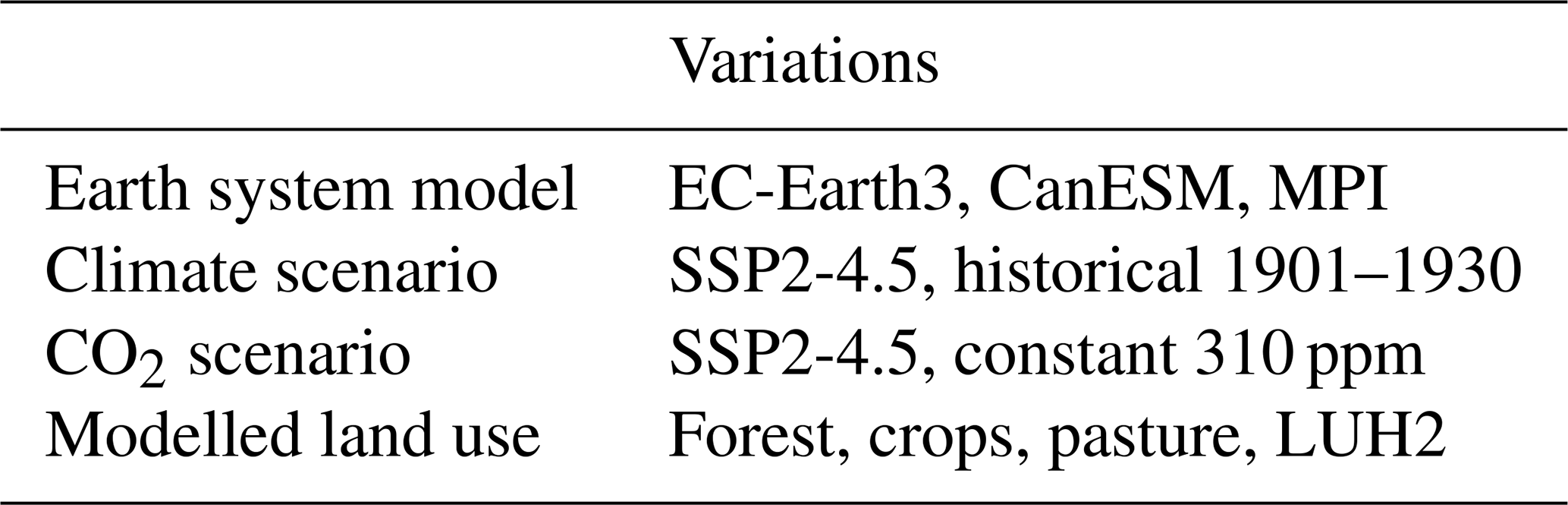
3.2 Case setup: runs and climate scenarios

We ran 48 global simulations with LPJ-GUESS, varying CO₂ concentration and climate scenarios from different climate models. The variations are presented in Table 3. The purpose of running different climate and CO₂ scenarios independently of each other was to distinguish between the effects climate change and CO₂ fertilization. Climate scenarios from three climate models were used to assess the results' sensitivity to model choice. LPJ-GUESS simulations began with a 500-year spin-up, and after that the actual simulations were run from 1900 to 2100. Model defaults for irrigation, fertilization and other cropland management options are used (Lindeskog et al., 2013; Olin et al., 2015).

The climatological data driving LPJ-GUESS are from the Coupled Model Intercomparison Project Phase 6 (CMIP6) simulations (Eyring et al., 2016) in the Earth System Grid Federation database. We used temperature, precipitation and solar radiation from three Earth system models (ESMs): EC-Earth3, CanESM and MPI-ESM. Citations of specific model variants and datasets are provided in Table S1 in the Supplement. These three model variants were chosen, as they give rather different results in terms of global mean temperature and precipitation: CanESM produces higher temperature and precipitation, MPI produces lower temperature and precipitation, and EC-Earth is between these. The datasets have been interpolated to 2°×2° grid by Climate Data Operators (CDO) using bilinear interpolation. Climate datasets used with LPJ-GUESS to parametrize the current version of CLASH were not bias-corrected. Biases in ESM results can have a large influence on ecosystem and carbon cycle modelling (Ahlström et al., 2017), but correcting for them can also introduce new uncertainties to scenarios of future climate (Maraun et al., 2017). Although averaging over large geographical areas is likely to reduce the biases' effect on CLASH parametrization, potential model users are advised to use parametrizations based on bias-corrected data, which we provide with subsequent model versions.

Each LPJ-GUESS simulation was based on one of two alternative climates: a warmer future climate (scenario SSP2-4.5) or colder historical climate (climate from years 1901–1930, randomly sampled). Likewise, two CO₂ concentration pathways were used: the SSP2-4.5 scenario or a constant concentration of 310 ppm. These four variations enable separating the effects of climate change and CO₂ fertilization when parametrizing the ecological module in CLASH. The three ESMs, on the other hand, provide three distinct parametrizations for CLASH, as averaging results from disparate models did not seem meaningful. In the following, we focus on the EC-Earth parametrization for brevity. The main climate variables of temperature and precipitation in each biome are presented in the Supplement.

Forests, crops and pastures were simulated separately at a global grid resolution of 2°×2°. That is, in forest simulations, only forest was grown at all the grid points. In crop simulations different crop types were grown, and in pasture simulations only grass was grown. To parametrize forest growth as a function of stand age, the forest simulations included forest stands planted in 20-year intervals from 1900 to 2000. In addition, one set of simulations with LUH2 land use (Hurtt et al., 2020) was run for primary ecosystem parametrization and model validation purposes.

Table 3 Scenario specifications for the LPJ-GUESS simulations.

3.3 Parameter fitting procedure

To parametrize the functions presented in Sect. 2, we used LPJ-GUESS output variables (such as vegetation carbon densities, litter and soil carbon stocks, NPP, crop yields, and annual forest fire probabilities) as dependent variables and climatological drivers (global mean temperature and CO₂ concentration) from the related climate scenarios as independent variables. All data were on an annual level. Three separate CLASH parametrizations were made, corresponding to the LPJ-GUESS runs driven with the EC-Earth3, CanESM and MPI climate scenarios. The separate CLASH parametrizations can be used to represent some of the variation that exists between ESMs regarding future climate change, as well as how these variations affect vegetation growth and terrestrial carbon stocks.

For static, linear equations (e.g. Eq. 3), ordinary least-squares fitting was used. For dynamic equations (Eqs. 4 and 6), the parameters were fitted by minimizing the sum of the squared errors between the LPJ-GUESS result and values simulated using the fit over the whole time frame (1900–2100). As this minimization problem is possibly non-convex, the parameter fitting was done in two steps: first using a global optimization algorithm to find a relatively good parametrization and then using this as a starting point for a local optimization algorithm to find the exact optimum.

To find a suitable form for each function, we started with a simple (e.g., linear) representation. If this was not sufficient to replicate the LPJ-GUESS results with sufficient accuracy, additional terms were added to the function. In the case of more complex formulae, particularly the relative forest growth of Eq. (5), a number of functional forms were tested in each case to ensure a suitable fit. The variations included, for example, polynomial, exponential, and power representation for the temperature effect or the inclusion or exclusion of interaction effects between the temperature and CO₂ concentration. The objective of the fitting procedure was to find functions that roughly emulate LPJ-GUESS. The final formulations are what is presented in Sect. 2.

3.4 Fits of forest growth and fires

The development of forest carbon density with stand age in a changing climate is shown in Fig. 2. The carbon density modelled with LPJ-GUESS is compared to the carbon density simulated using Eq. (4) with the fitted parameter values. The parametrization emulates the original LPJ-GUESS results well in all biomes and climate scenarios.

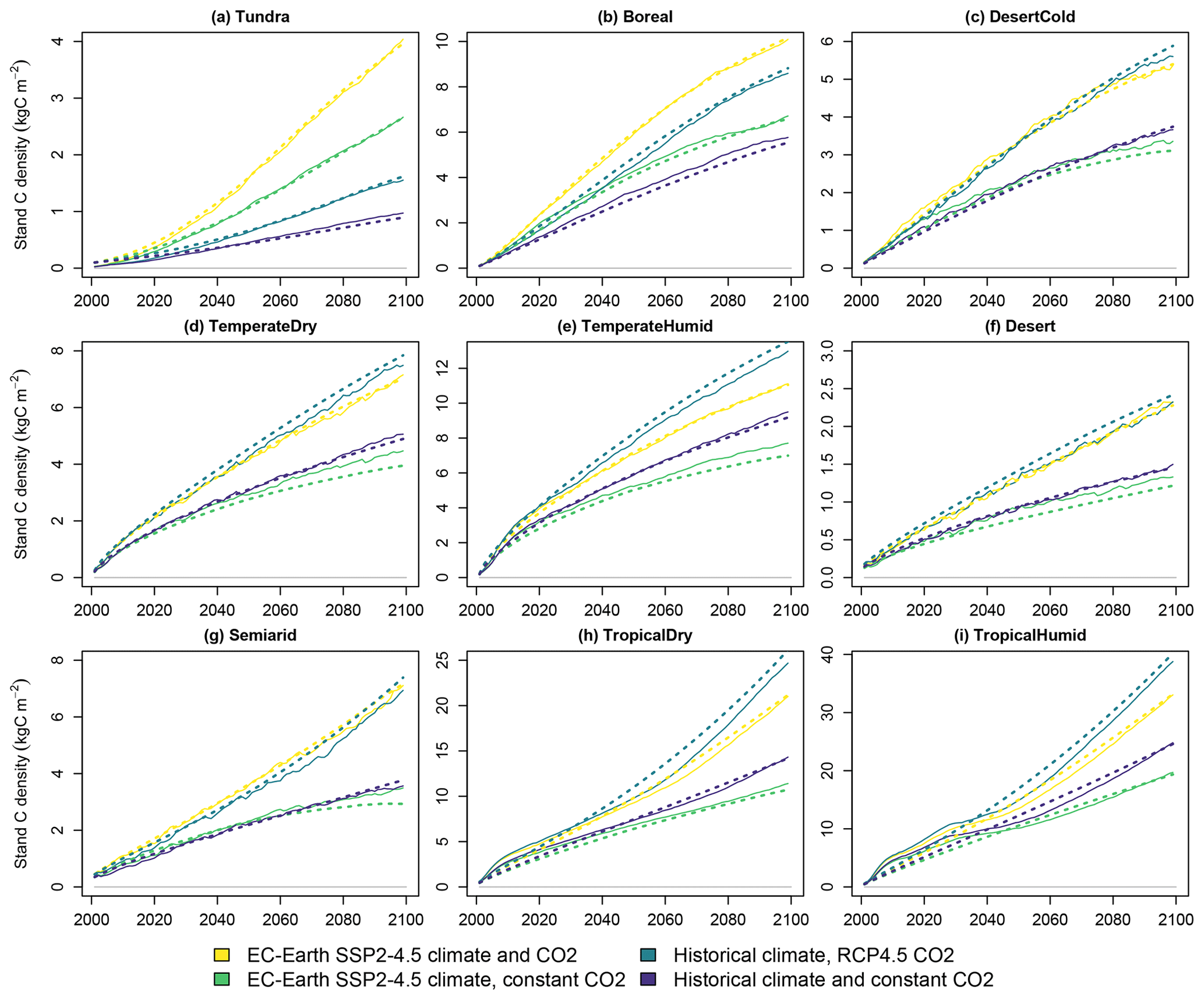
Figure 2 Forest stand carbon density in the four simulated climate scenarios with a stand planted in 2000. Solid lines indicate LPJ-GUESS simulations, and dashed lines indicate functions fitted to the results. The proximity of solid and dashed lines of the same colour indicates the goodness of fit. If the lines are close, CLASH emulates LPJ-GUESS well.

Forest growth, and how climate change affects it, varies across biomes. In colder biomes such as tundra and boreal biomes a warming climate increases forest growth considerably, whereas the opposite is true, although to a lesser degree, for the warmer biomes, particularly for temperate humid, tropical dry, and tropical humid biomes. Higher atmospheric CO₂ concentrations improve growth considerably in all biomes due to the CO₂ fertilization effect (Walker et al., 2021). This effect is relatively stronger in the warmer biomes than in the colder ones, which conforms with earlier analyses with LPJ-GUESS (Hickler et al., 2008).

Annual probabilities of forest fire from LPJ-GUESS and the fitted parametrization for an equation of the form (3) are displayed in Fig. 3. The fitted functions capture the overall level and in most cases the trend in the incidence of forest fires. Fire probabilities depend strongly on the biomes' climate. Generally, dry and warm biomes have more recurring fires than cold and wet ones. Tundra experiences a major increase in fire probability due to a warming climate. However, in some biomes, climate change does not affect fire prevalence strongly, and the changes are more driven by land-use change (Knorr et al., 2016). This effect is not captured by the explanatory variables of Eq. (3).

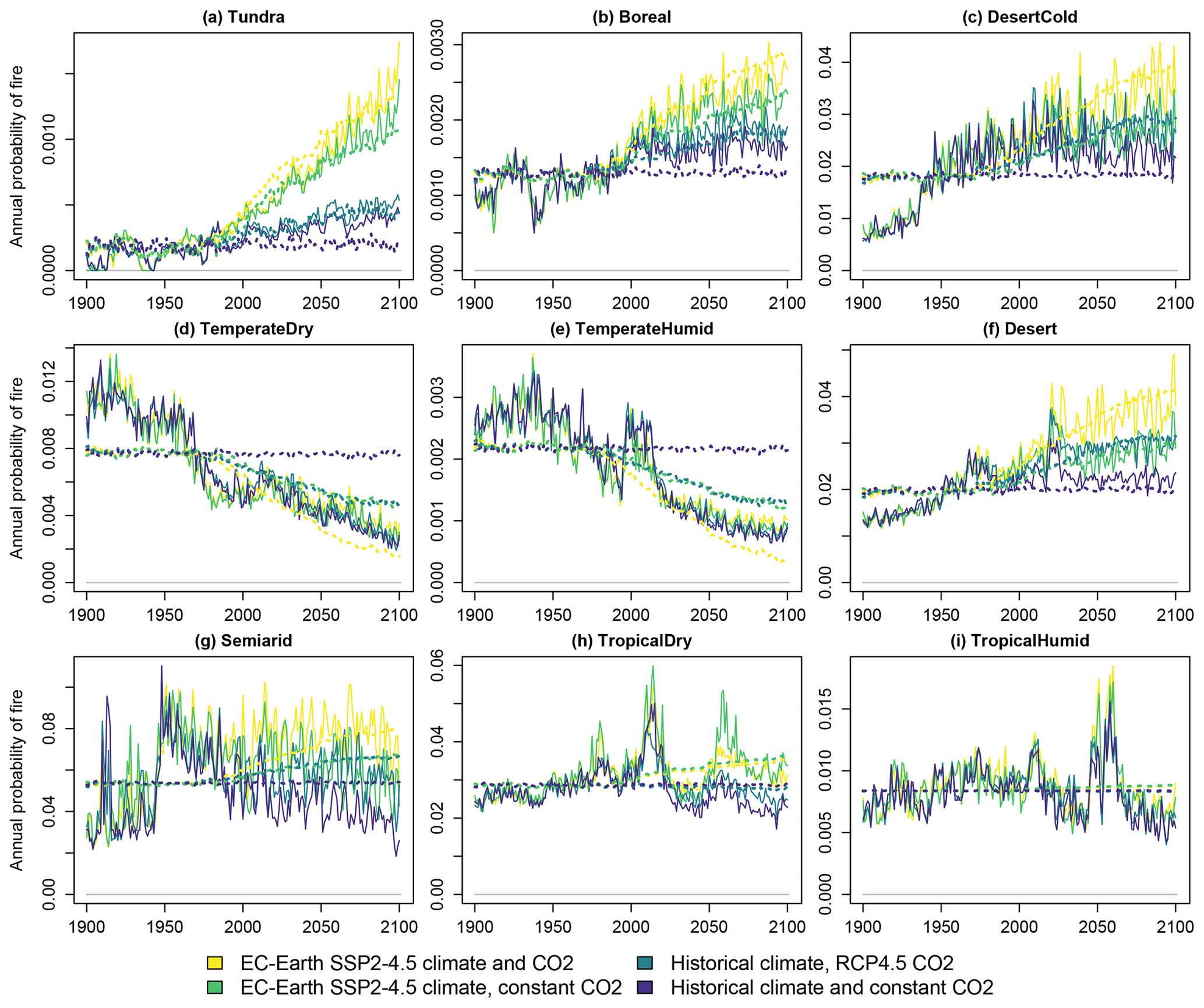
Figure 3 Average forest fire return times in the four simulated scenarios. Solid lines indicate LPJ-GUESS simulations, and dashed lines indicate functions fitted to the results.

3.5 Fits of vegetation carbon stocks

The carbon densities of natural vegetation, cropland and pastures are presented respectively in Figs. 4, 5 and 6. The linear model of Eq. (3), with temperature and CO₂ concentration as the explanatory factors, performs well in depicting the overall trends of the three vegetation types across scenarios and biomes. Cropland and pasture vegetation exhibit notable variation between consecutive years, which is not captured well by the statistical fit. However, as CLASH is primarily intended to be used at a 5- or 10-year time step, the inability to model annual fluctuations is not a major concern.

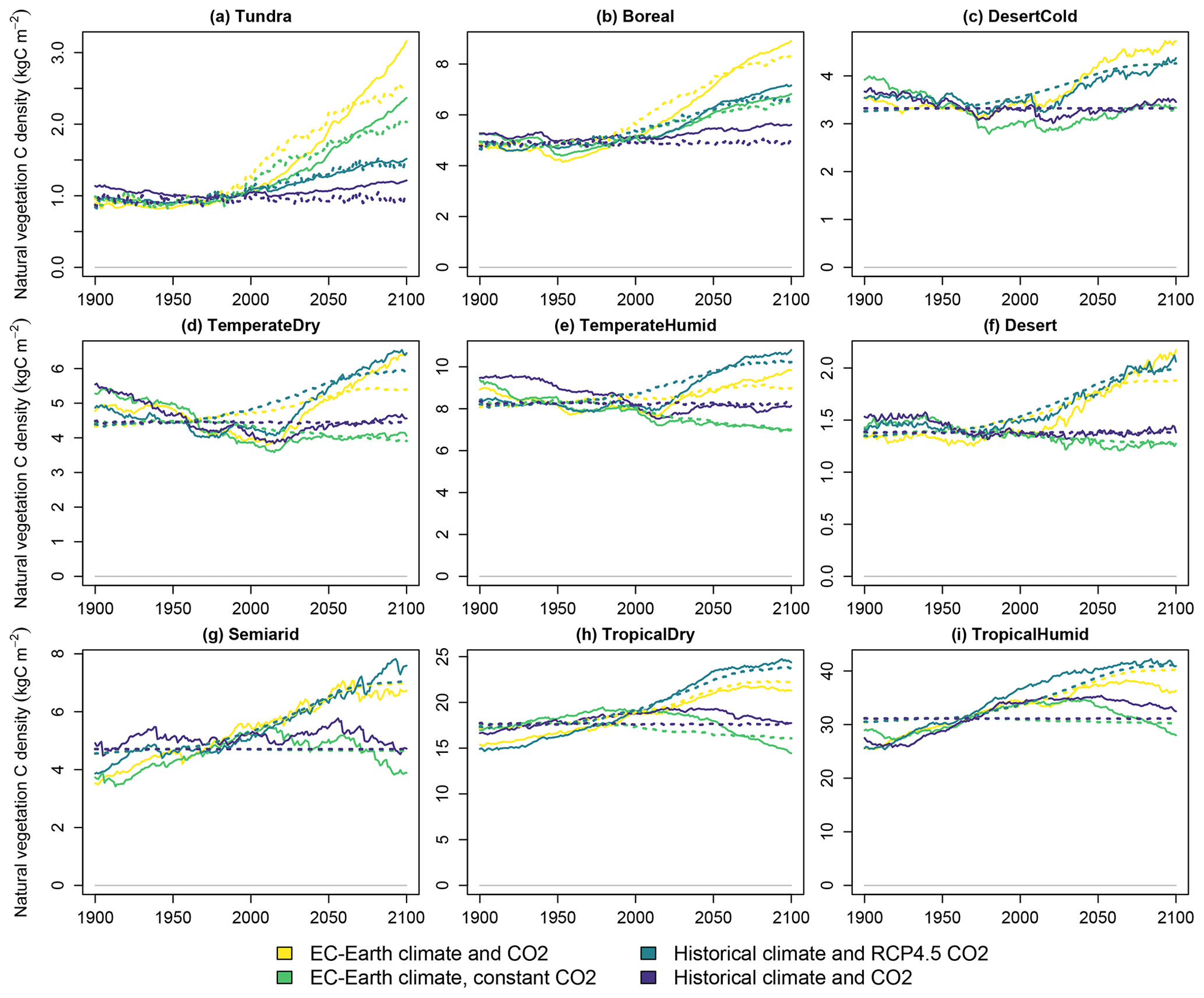
Figure 4 Carbon density in natural vegetation in the four simulated scenarios. Solid lines indicate LPJ-GUESS simulations, and dashed lines indicate functions fitted to the results.

The vegetation carbon stocks react strongly to climate change, and the magnitude of the effect depends on the biome. With a constant climate and CO₂ concentration the densities remain relatively constant, as can be expected. An elevated CO₂ concentration increases the vegetation carbon density through the CO₂ fertilization effect. A warming climate increases carbon density in the cold biomes but has a negligible or, in some cases, a small decreasing effect on the other biomes. These effects are generally well in line with previous observations and model experiments regarding the global greening (Piao et al., 2020).

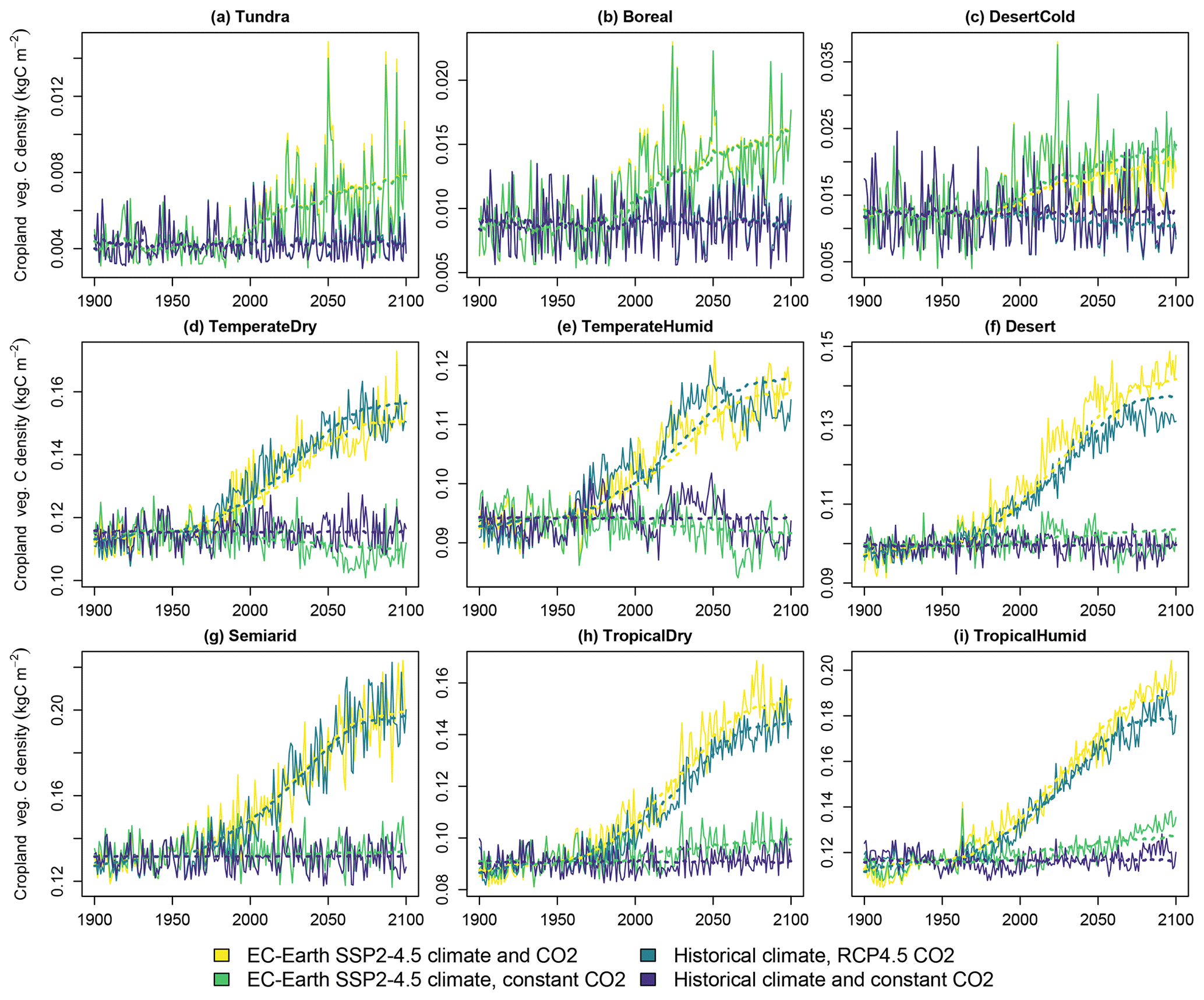
Figure 5 Carbon density in cropland vegetation in the four simulated scenarios. Solid lines indicate LPJ-GUESS simulations, and dashed lines indicate functions fitted to the results.

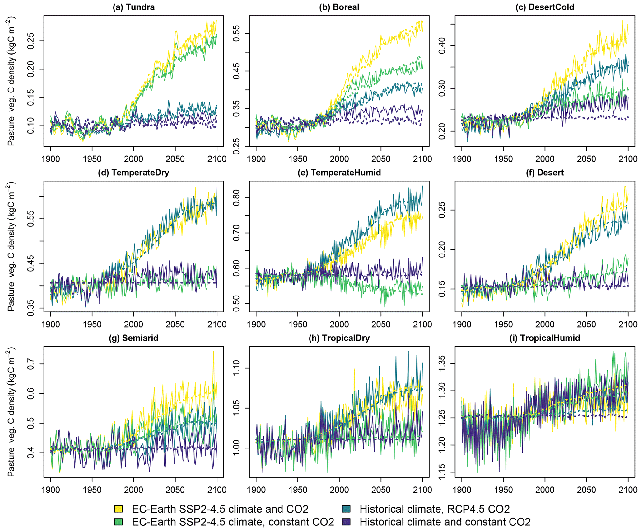
Figure 6 Carbon density in pasture vegetation in the four simulated scenarios. Solid lines indicate LPJ-GUESS simulations, and dashed lines indicate functions fitted to the results.

3.6 Fits of litter and soil carbon stocks

The litter and soil carbon stocks of forests, croplands and pastures are presented in the Supplement. The fitted functions mostly compare well against the LPJ-GUESS simulations in the four climate scenarios described in Table 3. Relative differences between the fitted functions and the original LPJ-GUESS simulations are the largest for cropland carbon stocks. This is because the functions for cropland and pasture share the same parametrization, as they both contribute to the herbaceous litter and soil stocks in CLASH. Pastures contain more carbon than croplands and, therefore, have more weight when the litter and soil carbon dynamics functions are parametrized by minimizing the squared error between the LPJ-GUESS result and the fit. Hence, the fit is better for pastures than croplands. For the same reason, however, inaccuracy in depicting cropland litter and soils does not notably affect the overall accuracy of CLASH in emulating LPJ-GUESS simulations. That is, as cropland litter and soil contain only a small part of the total carbon, and inaccuracy in depicting these stocks does not notably affect the overall accuracy of representing the total carbon stocks.

3.7 Fits of crop yield

The yield of the average crop is presented in Fig. 7. As mentioned previously, the colder biomes experience a notable increase in yields in a warming climate. Also, CO₂ fertilization improves yields notably. The statistical fits capture these changes well. The desert biome contains a discontinuity in the LUH2 cropland areas between the historical period and scenario after 2015, which is not captured by the fit.

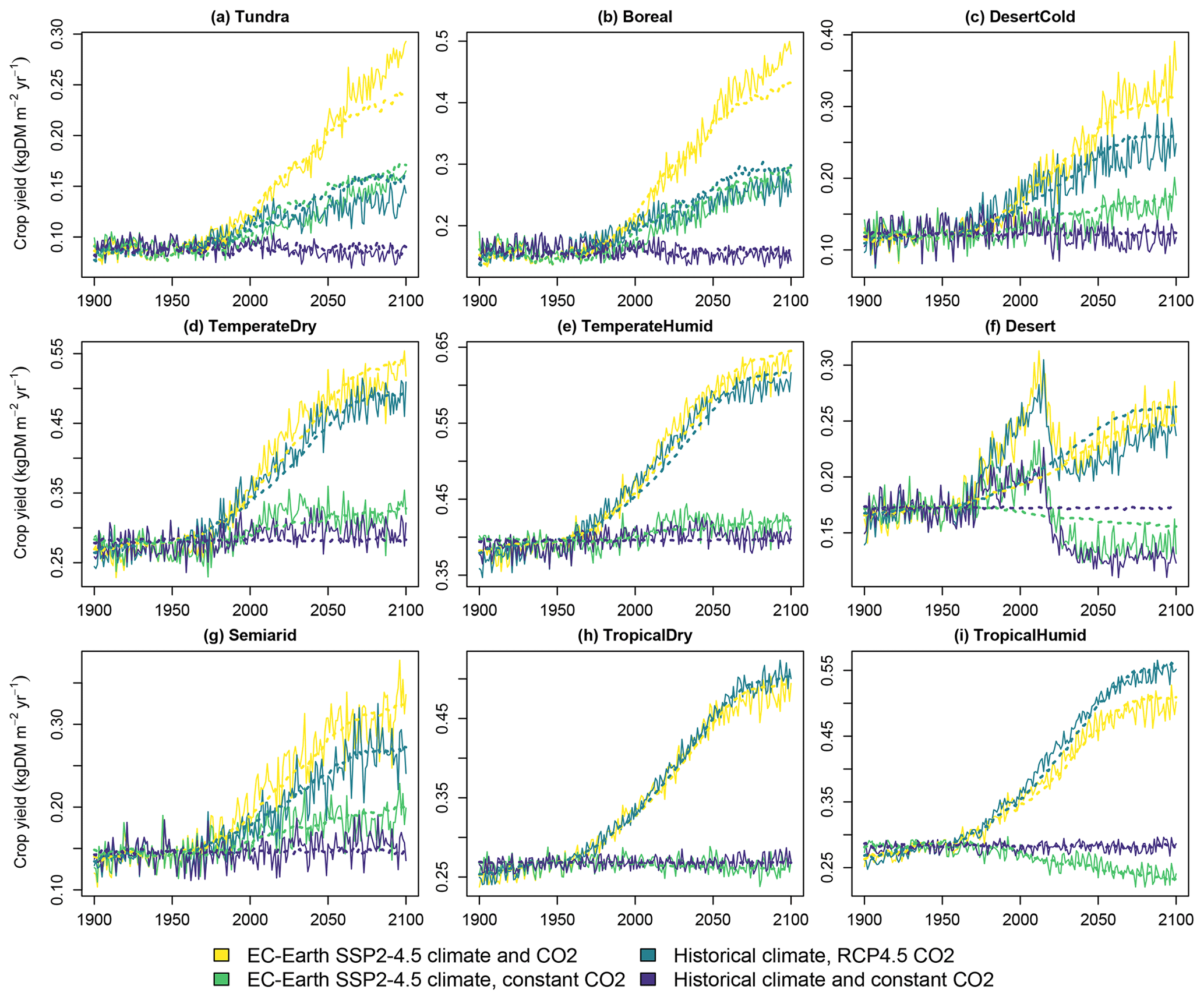
Figure 7 Crop yields in the four simulated scenarios. Solid lines indicate LPJ-GUESS simulations, and dashed lines indicate functions fitted to the results.

The CO₂ fertilization effect is notably strong on crop yields. In the temperate and tropical biomes, which comprise approximately 75 % of cropland area in 2020, the average crop yields increase respectively by 38 % and 57 % between 2000 and 2100 due to the CO₂ from the RCP4.5 concentration pathway. This is higher than the approximately 15 % to 30 % increase in a multi-model mean for four staple crops for the same concentration difference reported in Franke et al. (2020). However, in that study LPJ-GUESS produced the highest response to elevated CO₂ among the compared models, and our results are in line with these earlier LPJ-GUESS results. The model, along with LPJmL, has also previously been observed to produce a stronger CO₂ fertilization effect than other DGVMs (Müller et al., 2015). Hence, a high response to changes in the atmospheric CO₂ concentration is a property of LPJ-GUESS, which CLASH correctly replicates.

4 Validation

We validated CLASH by comparing its results to those from LPJ-GUESS in the SSP2-4.5 scenario. Both models used the LUH2 land-use patterns (Hurtt et al., 2020). CLASH parametrization based on EC-Earth3 was compared to LPJ-GUESS driven with the EC-Earth3 SSP2-4.5 scenario, and similar comparisons were done using MPI and CanESM climate scenarios. While the LUH scenario determines land area allocation between different uses, it does not specify how secondary forests are managed. Hence, to allow comparisons between the models, we applied forest management assumptions that lead to similar management. In the LPJ-GUESS LUH scenario, all forests were modelled without harvests. This behaviour was emulated in CLASH with an exogenous objective to maximize terrestrial carbon stocks in 2100, which effectively minimizes harvests.

The results of the validation experiment are shown in Fig. 8 with the EC-Earth3 climate scenarios. The models' results mostly align well with each other. The relative difference in the total terrestrial biosphere carbon stock ranges from 0.7 % to 3 % over the modelled examined time frame. The differences are larger for specific carbon stocks in certain biomes, such as vegetation in the tropical biomes.

Three main reasons can potentially explain differences in results between the two models. (1) The resolution of the aggregate biome-level representation in CLASH is coarser than compared to the 2°×2° grid applied in LPJ-GUESS. (2) Inaccuracies in the fitted functions describing the processes in CLASH could cause the results to differ. (3) The areas of different land uses in the LUH2 dataset are interpreted slightly differently in the two models, which also affect carbon stocks.

The main differences observed in Fig. 8 can be attributed to differences in resolution (1) and differences in the interpretation of LUH2 data (3). The first of these is inevitable, as CLASH describes the average growth, yield and carbon stocks over much larger areas than LPJ-GUESS. This was identified as the primary reason for the difference in vegetation carbon stock in the two tropical biomes. The problem could be remedied by applying a lower level of aggregation for the biomes, but this would increase the computational weight of the model.

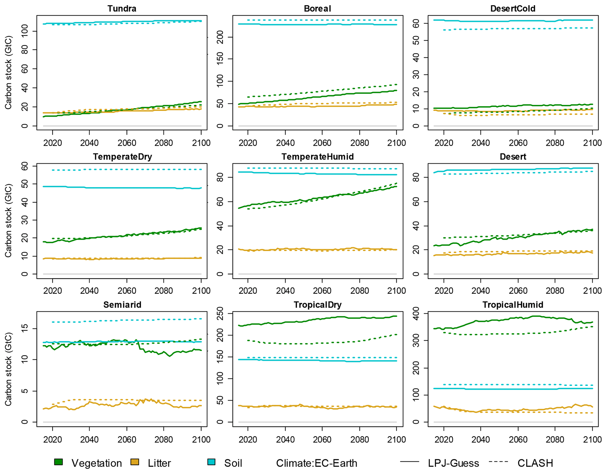
Figure 8 Validation of CLASH carbon stocks against LPJ-GUESS in the SSP2-4.5 scenario, separately for vegetation, litter and soil carbon in each biome. Solid lines indicate LPJ-GUESS results, and dashes indicate CLASH results.

Inaccuracies in the fitted functions (2) as a source of error could be reduced by trying to find functional forms that better emulate the LPJ-GUESS results. In general, however, the chosen functions and estimated parameters seem to replicate the LPJ-GUESS results relatively well. Cropland litter and soil carbon dynamics are an exception, but as these carbon stocks are minor compared to those of other land uses, their effect is small in the big picture.

Differences in the interpretation of the LUH2 dataset (3) imply that land allocation within the biomes differs slightly between the models. The original LUH2 data are at 0.33°×0.33° resolution. The area of land allocated to each use in each biome in CLASH is calculated directly from these data. However, for LPJ-GUESS, the data are re-gridded, and a 2°×2° grid is applied in the LPJ-GUESS simulations. Different gridding leads to differences in biomes' land-use allocations between the models. This difference particularly explains the differences in soil carbon stocks in the temperate dry and semiarid biomes, which have roughly 20 % more pasture area in CLASH.

Validations of CLASH fitted to the climate scenarios from CanESM and MPI models are presented in the Supplement (Figs. S9 and S10). These figures are qualitatively very similar to Fig. 8, which indicates that the different parametrizations of CLASH can emulate well the LPJ-GUESS results driven by climate scenarios from different ESMs. However, it is worth noting that the choice of climate model notably affects the level of certain carbon stocks in the LPJ-GUESS results. This is illustrated in Fig. 9 with the three alternative parametrizations of CLASH. Whereas across parametrizations the carbon stocks are similar for most biomes, there is a particularly notable difference in the tundra biome, where the use of the CanESM climate scenario produces significantly larger carbon stocks for all three carbon pools. This can be explained by the higher temperature in the CanESM scenario compared to the other two climate scenarios. The higher temperature means greater vegetation growth, more litter input and hence larger soil carbon stocks.

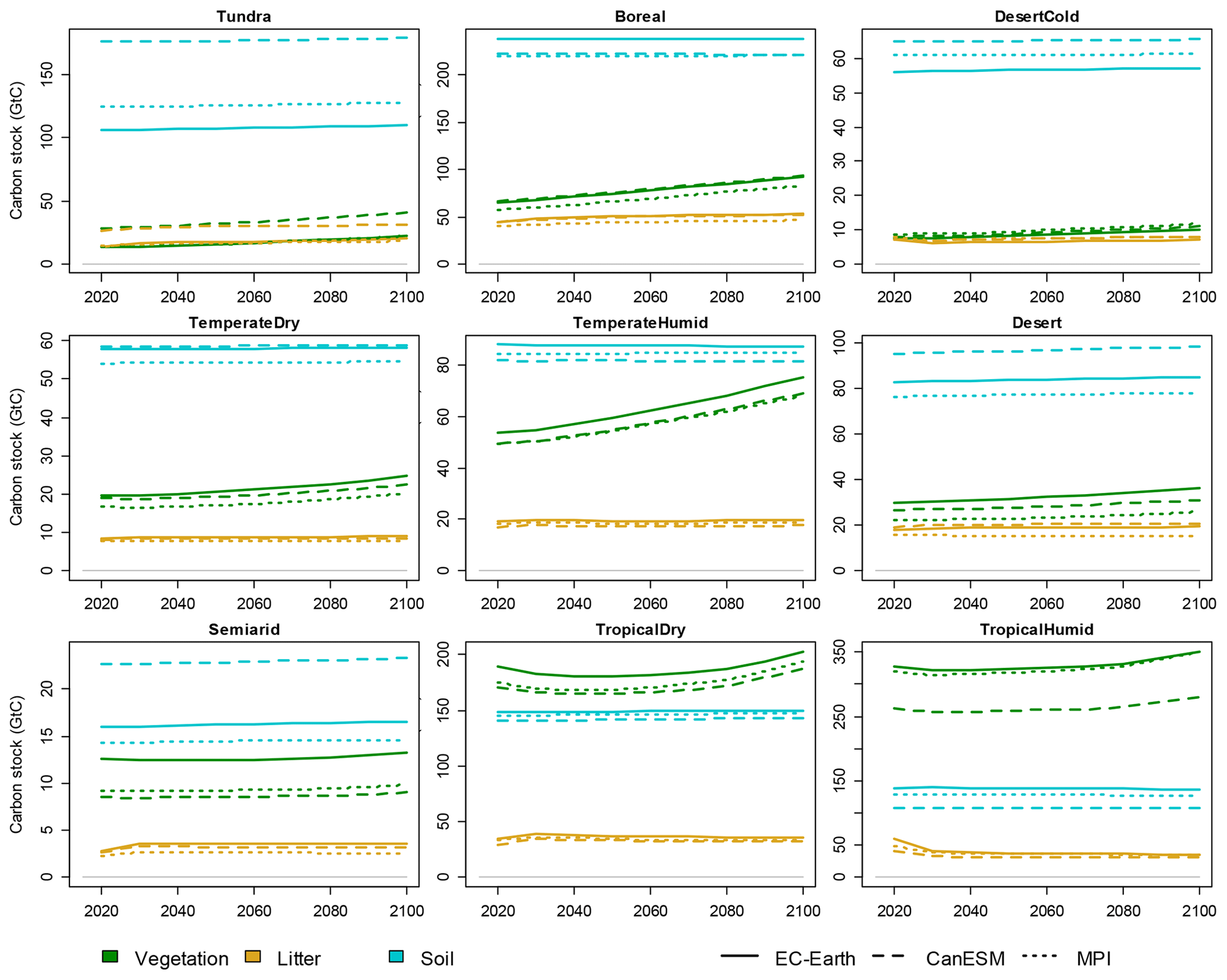
Figure 9 Vegetation, litter and soil carbon stocks in a SSP2-4.5 scenario, modelled by CLASH parametrized against LPJ-GUESS-results-driven climate scenarios from EC-Earth (solid lines), CanESM (dashed lines) and MPI (dotted lines) models.

Comparing CLASH to future scenarios from other models is not as straightforward, as each model study has its own modelling mechanisms and set of assumptions that might be difficult to replicate in CLASH. In particular, given that CLASH is a biophysical model, it does not represent the markets and policies that drive the production of land-use products. Nevertheless, we make a simple comparison by fixing the land-use areas of CLASH to the LUH2 SSP2-4.5 scenario and compare the crop and wood production to FAO statistics, IAM scenarios and forest sector models. This comparison is presented in Fig. 10.

Crop production provides a straightforward comparison, as cropland area determines crop production directly in CLASH. We compare CLASH results to FAO statistics, FAO's future of food and agriculture scenarios (FAO, 2018) and SSP2-4.5 scenarios from five different IAMs (Riahi et al., 2017). CLASH crop production is very close to the FAO statistics and at the upper end of the scenarios around 2020. Crop production grows slightly slower than in the FAO scenarios and notably slower than in the SSP scenarios, however. The reason for this divergence is strongly increasing energy crop production in the IAM scenarios. Energy crops have potentially higher yields than food crops, which leads to larger production with the same cropland area. However, food crop production in most of the IAM scenarios remained slightly below the CLASH crop production.

Comparing wood harvests is not as straightforward, as managed forest area can yield very different wood harvests, depending on harvesting intensity. Therefore, for this comparison, we additionally required CLASH to produce the same amount of industrial roundwood (logs and pulpwood) than in the demonstration case of Sect. 5. This demand scenario was then compared to FAO statistics (also including the category “Other industrial roundwood”) and a recent comparison of forest-sector model (FSM) scenarios by Daigneault et al. (2022). The CLASH demand scenario matches the FAO statistics well and is for the most part slightly higher than the harvests in the FSMs. Further comparisons are difficult due to seemingly different definitions of forest land, with FSMs being based on FAO statistics and CLASH on LUH2. This results in differences of forest land area and thereby also forest carbon stocks. Yet, as a separate comparison, the forest carbon stocks in CLASH fall in the range reported in a recent review of terrestrial biosphere models (Seiler et al., 2022), based also on the LUH2 land-use categorization.

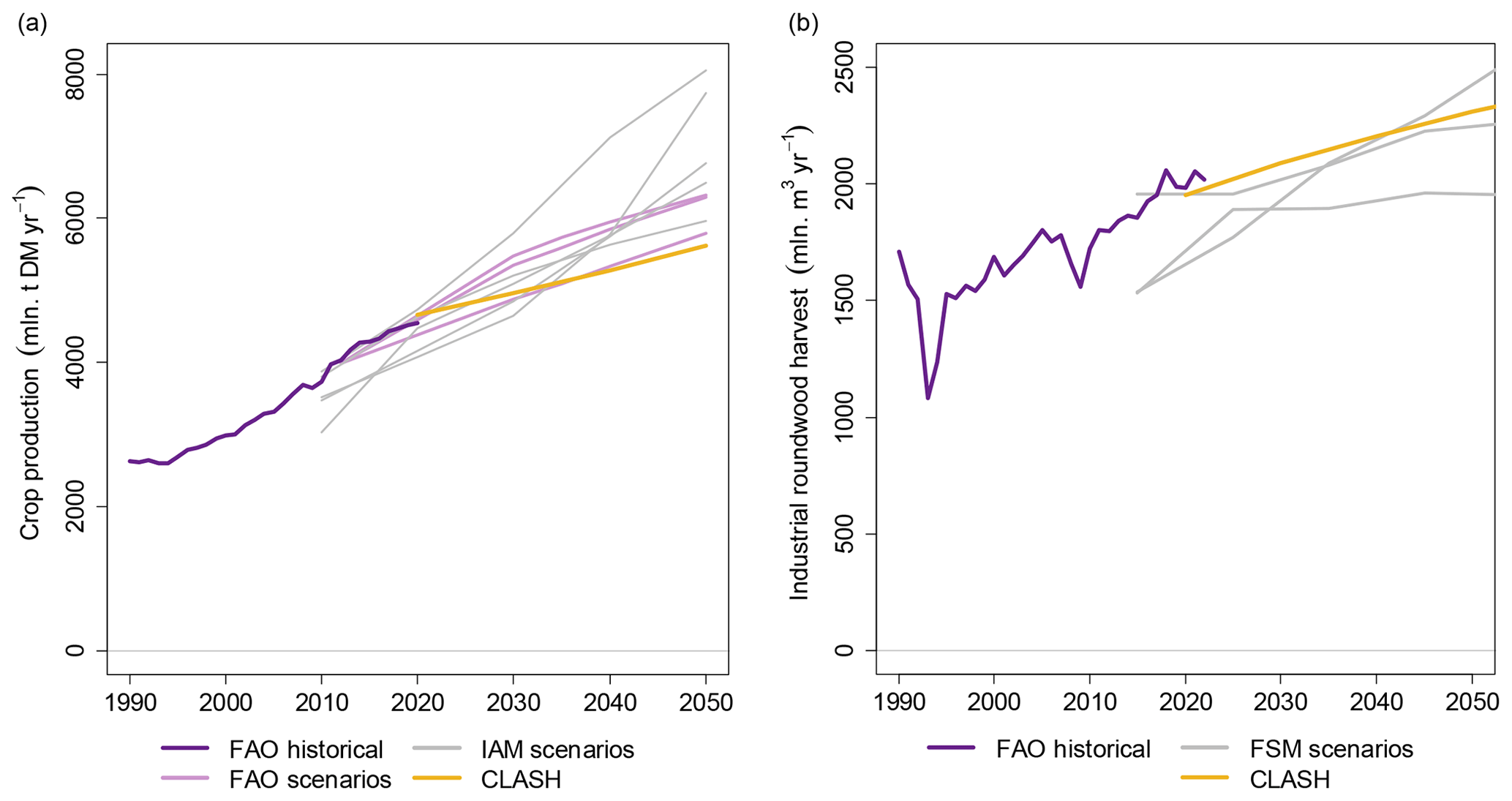
Figure 10 Comparisons of crop production (a) and industrial roundwood harvests (b) between CLASH, FAO and SSP2-4.5 scenarios from either IAMs for crop production or forest sector models (FSMs) for wood harvests.

5 Analysing trade-offs between carbon storage and production

To demonstrate the behaviour and possible use cases of CLASH, we explored how varying the future demand for different land-use products affects the global terrestrial carbon sink during the 21st century. In the example, CLASH is run subject to an exogenously given objective: maximize the terrestrial carbon stock in 2100 by allocating managed lands between the biomes, while satisfying an exogenously given demand scenario for agriculture and forestry products. As this problem setting does not represent the drivers determining real-world land-use decisions, the analysis should be seen as a simple demonstration of the model through scenarios that would still be physically possible.

There is a trade-off between storing carbon in the biosphere and producing land-intensive products: more production usually implies less storage (Erb et al., 2018). Examining this trade-off can help understand the physical limitations of the land-use sector's contribution towards mitigating climate change, e.g. to reach the Paris Agreement's 1.5 °C target (Roe et al., 2019). Given these physical limitations in land use, this trade-off can be seen as a production-possibility frontier between carbon storage and the supply of land-use products (Pingoud et al., 2018). Here, we use CLASH to analyse this problem as an example of how the model can be utilized in practice.

In this demonstration, CLASH is allowed to freely allocate land between cropland, pastures, and secondary forest across all biomes. The areas of other land uses develop according to the SSP2-4.5 LUH scenario (Hurtt et al., 2020). We vary the future demand of four product categories: crops (for direct human consumption), animal products (meat, milk and eggs), wood products (timber and pulp wood) and bioenergy (energy crops and energy wood).

The model is first solved in a baseline scenario, in which the demand for each product category follows the SSP2-4.5 scenario from 2020 to 2100 (Riahi et al., 2017), denoted as D_BL(t). Then, we vary the demanded quantity of each product category at a time from the baseline, so that the demand D(t) deviates gradually from the baseline until a variation m of ±10 % or ±50 % is reached by 2100:

$$\begin{array}{}\text{(12)}& D\left(t\right)=D_{\mathrm{BL}}\left(t\right)\cdot \left(\mathrm{1}+m\cdot {\displaystyle \frac{t-\mathrm{2020}}{\mathrm{2100}-\mathrm{2020}}}\right).\end{array}$$

Hereafter, the demand scenarios are referred to as very low (−50 %), low (−10 %), high (+10 %) and very high (+50 %) demand.

Figure 11 shows how changes in the demand for each product category affect the global carbon stock and net CO₂ uptake of terrestrial ecosystems in 2100. The stocks respond almost linearly to changes in the demanded quantities. Altogether, the change in global carbon stocks between 2020 and 2100 ranges from −90 to +310 GtC across the demand scenarios or −156 % to +94 % relative to the baseline increase of +160 GtC. Variation in animal product demand is responsible for the extremes of the range, and when measured per tonne of product, the variation affects the average CO₂ uptake 7–8 times as strongly as variation in the crop or bioenergy demand and 15 times as strongly as variation in wood demand. The very high animal product demand scenario is the only scenario where terrestrial ecosystems are a net emitter instead of a net sink.

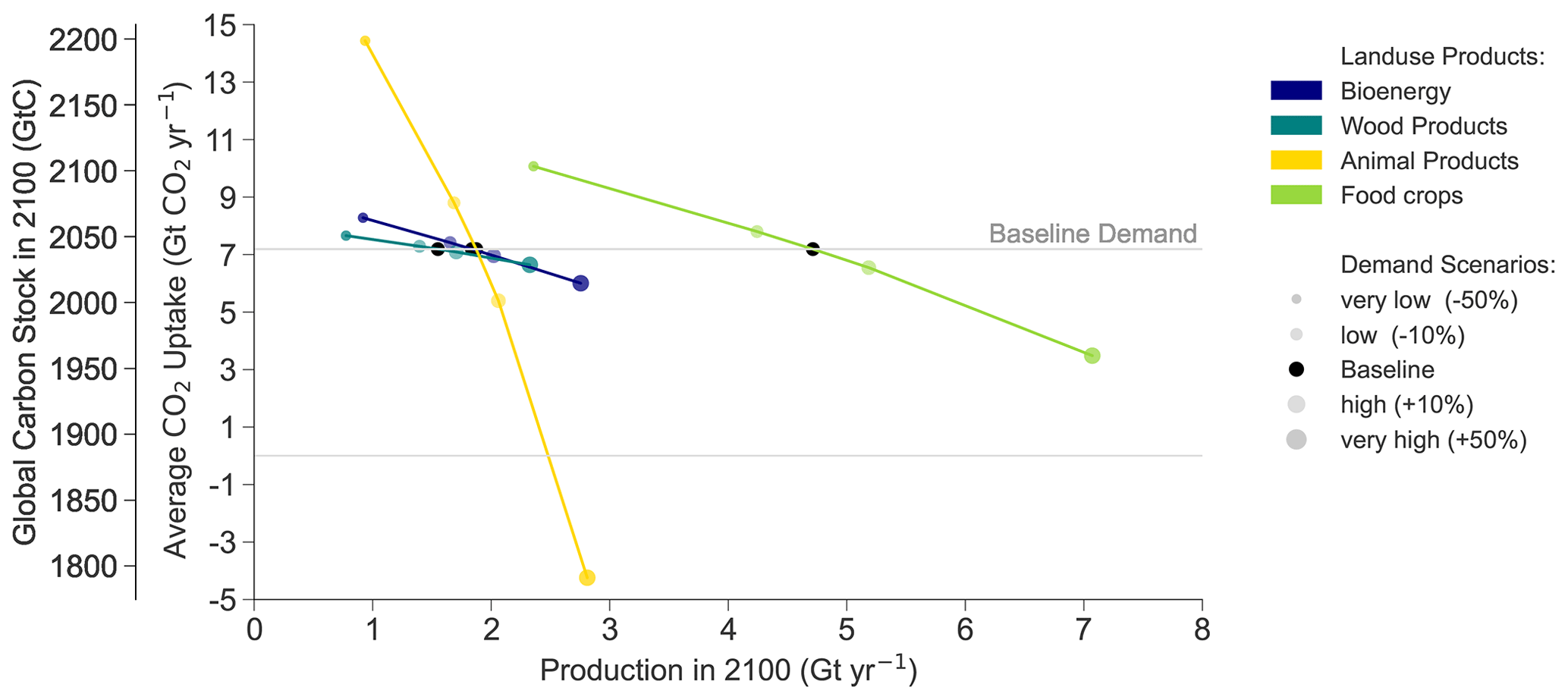
Figure 11 The production-possibility frontier between carbon storage (left y axis), terrestrial CO₂ uptake (right y axis), and the production of different land-use products (x axis) for food crops, animal products (meat, milk and eggs), wood products (logs and pulp wood) and bioenergy (crops and logging waste). The carbon storage in the baseline demand scenario is indicated with a horizontal grey line. The demand variations are represented with point size and colour: different product categories are indicated by colour, and the point size indicates the relative deviation in 2100 from the baseline demand (the bigger the point size, the bigger the demand). The slope of the line connecting the points indicates the sensitivity of global carbon stock to a change in demand per tonne of product.

Demand variations cause land-use conversions between cropland, pastures and secondary forests (Fig. 12a). High demands for crops, animal products or bioenergy are satisfied by converting additional secondary forest to agricultural land, while in the low-demand scenarios unused agricultural land can be converted to secondary forests to increase the global carbon stock. Croplands and pastures are mostly allocated to tropical and boreal biomes (Fig. 12b). Cropland and pastures together make up 47 %–49 % of total land area in 2050 and 36 %–68 % in 2100. The loss of primary ecosystems from 2020 to 2100 amounts to 15 %–24 %. The sensitivity of the loss of primary ecosystems for animal product demand is 10 times stronger than that of wood demand, 33 times stronger than that of bioenergy demand and 129 times stronger than that of food crop demand.

In our illustrative case, the production of crops is mostly allocated to the tropical dry, boreal and temperate humid biomes. Pastures are mostly allocated to tropical biomes, with boreal land areas serving as fallback for very high animal product demand. Wood demand is satisfied on the one hand by large-scale forestry in boreal forests, with moderate forestation during the first half of the century and intensive harvest during the second half of the century. On the other hand, wood is delivered by constant intensive harvest of the temperate humid zones, while cut-down forest is not reforested but converted into cropland. Hence, temperate biomes' carbon stocks decrease the most during the century (Fig. 12b).

The results suggest that – when assessed purely in terms of biophysical properties – the tropical and tundra biomes have a relative advantage in storing carbon over producing crops and timber but are heavily affected by high animal product demands (Fig. 12b and c).

Due to land-use change and intensive wood harvests, the temperate humid secondary forests' area-weighted mean forest age drops from 84 years (2020) to below 10 years in 2100. The boreal forest age decreases from 101 years in 2020 to 65 years in 2100. Meanwhile, the tropical humid biome's mean age of secondary forests increases from 36 years in 2020 to 109 years in 2100, and the tundra biome's mean age of secondary forests increases from 80 years (2020) to 147 years in 2100 (Fig. 12c).

Notably, the maximization of global carbon storage subject to the global demand constraints leads to a strongly polarized land allocation between the biomes. Economic factors (such as production costs, trade policies, security of supply concerns and the value of ecosystem services) are not considered in this optimization problem. Doing so would alter regional relative advantages between carbon storage and production and lead to a different global land allocation.

The CH₄ and N₂O emissions from agricultural activities reach 14–33 Gt CO₂ eq. yr⁻¹ between 2090 and 2100 (Fig. 12d), of which 63 %–73 % are from animal husbandry. In most scenarios, the terrestrial carbon sink in 2100 (−20–+6 GtCO₂ eq. yr⁻¹) is not large enough to compensate fully for the agricultural non-CO₂ emissions, and, therefore, land use is a net source of GHG emissions in 2100. In the very high animal product demand scenario, terrestrial ecosystems already become a net emission source by 2050.

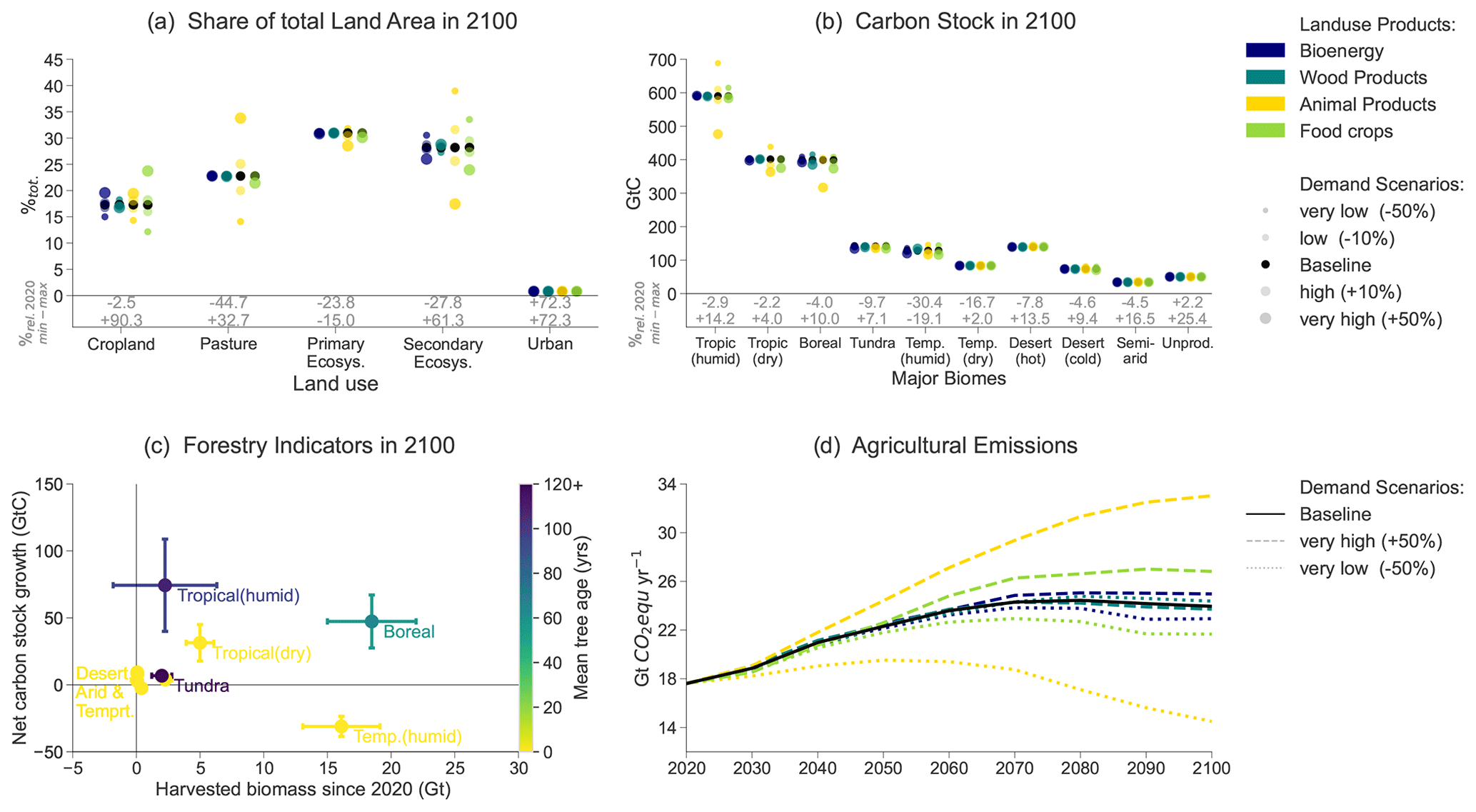
Figure 12 (a) Share of total land area in 2100 (%_tot.) and relative change since 2020 (%_rel.) per land-use type in all scenarios. (b) Total carbon stock in 2100 (GtC) and relative change (%_rel.) per biome in all scenarios. (c) Total harvested biomass (Gt) and net carbon stock growth (GtC) for period 2020–2100 and area-weighted-average tree age in 2100 (years) per biome averaged over the scenarios (error bars). (d) Evolution of agricultural CH₄ and N₂O emissions from crop cultivation, enteric fermentation and manure management (Gt CO₂ eq. yr⁻¹) for baseline and extreme demand scenarios. In panels (a) and (b), the point size indicates the relative deviation in 2100 from the baseline demand for the product category indicated with the colour. In panel (d), the line type represents the relative variation in demand for the product category indicated with the colour.

Altogether, the large effect of animal products on climate, land area and ecosystems supports the view that reducing their consumption could be an effective means to mitigate climate change (Jarmul et al., 2020; Hayek et al., 2021). Earlier research has also suggested that the relocation of croplands (Beyer et al., 2022) and increasing carbon storage in forests (Sohngen and Mendelsohn, 2003) are effective ways to mitigate climate change. All these effects can be identified in our illustrative analysis conducted using CLASH.

6 Conclusions

CLASH is a lightweight biophysical model that represents land use at an aggregate level of 10 biomes, each divided into six land-use classes. Vegetation growth and ecosystem carbon dynamics respond to climate change in CLASH, and the model keeps track of terrestrial carbon stocks and, thereby, also of terrestrial CO₂ emissions and sinks. CLASH has been specifically designed to be hard linked with IAMs. It can be incorporated into models formulated as linear or nonlinear programming problems, and it can be run under intertemporal optimization. In this role, CLASH can be used to optimize global agriculture and forestry and their climatic impacts over a multi-decadal timescale. Hence, it can help in evaluating the possible role that land use might have in mitigating climate change.

When integrated with an IAM, CLASH provides the annual production of land-use commodities (food and other biomass for energy and materials), the change in terrestrial CO₂ stocks and GHG emissions from agriculture. The IAM should provide the demand for these products, as well as any costs, policies and other societal constraints that affect land use. As such, CLASH would depict land use from a biophysical perspective, whereas the IAM provides the motivation for how the land should be used and managed.

If the IAM has a built-in climate module, it can provide the future CO₂ concentration and temperature change for the CLASH ecological module, while CLASH can calculate the net carbon exchange of terrestrial ecosystems. However, in such a setup, it is important to note a likely discrepancy between the climate module's carbon cycle and the carbon stocks represented by CLASH. In particular, the climate module should not represent the carbon exchange between atmosphere and terrestrial ecosystems, as CLASH accounts for terrestrial carbon stocks and the fertilization effect from elevated CO₂ concentrations. Further model development might be needed to replace relevant parts of the IAM climate module (or an external simple climate model) with associated outputs from CLASH to ensure consistency between the two parts.

CLASH could be easily re-parametrized to alternative geographic resolutions and time steps to achieve compatibility with a specific IAM or to represent political borders, which would be necessary for including agricultural, climate, and ecosystem protection and other policies relevant for land use. It would also be possible to use CLASH as a pure simulation model, that is, without any optimization problem. However, this might be impractical due to the number of free variables and the equation structure of the model. For this reason, we specified an external optimization problem of carbon stock maximization in Sect. 5.

The role of land use in climate change mitigation has been extensively analysed from various perspectives (e.g. Harper et al., 2018; Roe et al., 2019; Daioglou et al., 2019; Daigneault et al., 2022; Roebroek et al., 2023), and the topic's policy relevance has recently increased due to the grown interest in maintaining and enhancing land-based carbon sinks (Rockström et al., 2021; Griscom et al., 2017). Our demonstration of CLASH in Sect. 5 highlights the model's capacity to depict several well-known mechanisms through which land use can contribute to climate change mitigation, including reducing the consumption of animal products (Jarmul et al., 2020; Hayek et al., 2021), relocating croplands (Beyer et al., 2022) and increasing carbon storage in forests (Sohngen and Mendelsohn, 2003).

Due to its simplicity, CLASH cannot match the accuracy or detail of sectoral models, which have been soft linked with IAMs (e.g. Fricko et al., 2017; Favero and Mendelsohn, 2014). CLASH's relative advantages are its light computational burden and broad scope. It can be hard linked to IAMs and run under intertemporal optimization to provide a comprehensive depiction of global land use, terrestrial carbon stocks and their bi-directional interaction with the climate. We believe such hard linking of CLASH and an IAM would be helpful in examining the optimal role of land use in mitigating climate change, in providing food and biogenic raw materials for the economy, and in conserving primary ecosystems.