Challenges of constructing and selecting the “perfect” boundary conditions for the large-eddy simulation model PALM

We present the process of and difficulties in acquiring the proper boundary conditions (BCs) for the state-of-the-art large-eddy simulation (LES)-based PALM model system. We use the mesoscale Weather Research and Forecasting (WRF) model as a source of inputs for the PALM preprocessor and investigate the influence of the mesoscale model on the performance of the PALM model. A total of 16 different WRF configurations were used as a proxy for a multi-model ensemble. We developed a technique for selecting suitable sets of BCs, performed PALM model simulations driven by these BCs, and investigated the consequences of selecting a sub-optimal WRF configuration. The procedure was tested for four episodes in different seasons of the year 2019, during which WRF and PALM outputs were evaluated against the atmospheric radiosounding observations. We show that the PALM model outputs are heavily dependent on the imposed BCs and have different responses at different times of the day and in different seasons. We demonstrate that the main driver of errors is the mesoscale model and that the PALM model is capable of attenuating but not fully correcting them. The PALM model attenuates the impact of errors in BCs in wind speed, while for the air temperature, PALM shows variable behavior with respect to driving conditions. This study stresses the importance of high-quality driving BCs and the complexity of the process of their construction and selection.

1 Introduction

Interest in studying the urban atmosphere and climate has been present since the last century, and according to Mills (2014) it started with the work of Howard (1818). Due to the increasing number of city inhabitants and their impact on urban climate (Oke et al., 2017) and many other (scientific and commercial) relevant factors (Souch and Grimmond, 2006), this field of study will remain a key focus for researchers in the future. Characteristics of urban areas and climate (e.g., urban heat islands (UHIs), altered winds, and air quality) have been explored by many scientists (e.g., Arnfield, 2003; Mirzaei, 2015; Oke et al., 2017; Masson et al., 2020). Even though many challenges have been encountered while researching urban areas (e.g., Arnfield, 2003; Blocken, 2018; Kubilay et al., 2020), there are several methods used for studying them (e.g., Blocken, 2015; Toparlar et al., 2017), among which computational fluid dynamics (CFD) models are one.

A particular asset of the CFD method is that it allows for detailed physics-based analysis of the urban climate and urban physical phenomena (Kubilay et al., 2020), i.e., for scales below 2 km (Blocken, 2018). CFD models are versatile and appropriate for studying flow around buildings, pedestrian wind, vegetation-cover-related topics, etc. (e.g., Toparlar et al., 2017; Blocken, 2018). While using CFD models for numerical simulations, one needs to consider which turbulence model to use. According to Blocken (2018) and Kubilay et al. (2020), CFD models mostly rely on Reynolds-averaged Navier–Stokes (RANS) or large-eddy simulation (LES) turbulence models, whose qualities and weaknesses have been the topic of many studies (see, e.g., Hanjalic, 2005; Blocken, 2015, 2018; Maronga et al., 2019). In recent years, despite their higher computational cost, LES models have become popular among researchers and modelers due to their higher accuracy and ability to thoroughly capture the physical processes within the urban atmosphere.

Currently, the scientific literature uses two major open numerical models based on LES with advanced urban parameterizations that allow scientists to study urban areas at a very high resolution: uDALES (Suter et al., 2022) and the PALM model system, originally known as the Parallelized Large-eddy Simulation Model (Maronga et al., 2020). Today, PALM solely refers to the model name because it has been extended with a RANS core (Maronga et al., 2020). In general, the PALM model has been the subject of many studies conducted for different purposes (e.g., Letzel et al., 2008; Resler et al., 2017; Heldens et al., 2020; Fröhlich and Matzarakis, 2020; Gehrke et al., 2021; Pfafferott et al., 2021). Despite the advantages and the level of detail it provides, there are still many limitations to it, some of which are mentioned in the earlier studies, but not in all of its components and applications. One segment, which to the best of our knowledge has not been thoroughly investigated, is related to the issue of choosing the most suitable time-dependent meteorological boundary conditions for running a given PALM simulation.

While being capable of utilizing the standard cyclic boundary conditions (Maronga et al., 2015, 2020) and applying them to homogeneous and idealized setups (e.g., Gronemeier et al., 2017, 2021; Resler et al., 2017; Kurppa et al., 2018; Řezníček et al., 2023), PALM offers a so-called one-way offline nesting system, which enables it to take meteorological conditions from the mesoscale meteorological models and employ them throughout the entire PALM simulation (Kadasch et al., 2021). The application of such a system is most significant in the case of studying the atmosphere of a real, complex, and densely built urban environment. Furthermore, the utilization of boundary conditions that are as good and as realistic as possible during the PALM simulations is of high importance, especially in model validation studies and comparisons with observations, in which we strive to eliminate other possible sources of errors beyond the model formulation and implementation (see, e.g., Resler et al., 2021). A natural consequence of the impact of the boundary (and initial) conditions on the microscale simulation is the fact that any validation involves the full coupling of the driving mesoscale model (e.g., WRF, the Icosahedral Nonhydrostatic Weather and Climate Model (ICON; Zängl et al., 2015), or the Consortium for Small-scale Modeling (COSMO) and accordingly their driving data) and the high-resolution model, i.e., PALM. While providing the driving data to the microscale model, the errors and uncertainties coming from the mesoscale model are introduced, and their magnitude or origin is not always known. Therefore, without separating the errors that arise from the mesoscale and microscale models, one could be deceived into placing the responsibility on an erroneous representation of some microscale model processes, while the true origin of the errors might come from the mesoscale model and driving fields it provides. Hence, further development of the microscale model (e.g., PALM) could target the wrong part or process and consequently introduce overcorrecting model adjustments, in the end obtaining better results for the wrong reason.

Up to now, several mesoscale model outputs have been used as drivers for the PALM model simulations, namely, the Consortium for Small-scale Modeling (COSMO; Baldauf et al., 2011), the Meteorological Cooperation on Operational Numerical Weather Prediction (MetCoOp) Ensemble Prediction System (MEPS; Bengtsson et al., 2017; Müller et al., 2017), ALARO and/or AROME (Termonia et al., 2018), and the Weather Research and Forecasting (WRF) model (Skamarock et al., 2019), three of which (COSMO, MEPS, and ALARO and/or AROME) are not publicly available. A description of the processing tools for initial and boundary condition (IBC) creation made for the COSMO model can be found in Kadasch et al. (2021) and Kurppa et al. (2020) for the MEPS modeling system. Furthermore, the ALARO and/or AROME has been used for PALM initialization in a case study done by Zuvela-Aloise et al. (2022). On the other hand, given the fact that the WRF model is publicly available and widely used among researchers, several different preprocessors have been developed, including the WRF interface, which is part of the PALM distribution (Resler et al., 2021, and most recently by Vogel et al., 2022). Since this work covers the topic of finding the optimal choice of WRF-modeled BCs, we only considered the studies which employed WRF boundary conditions and looked through their respective choices of WRF model setups (see, e.g., Resler et al., 2017; Belda et al., 2021; Resler et al., 2021; Vogel et al., 2022). Each of these studies has implemented a particular WRF model setup which differs in the parameterization bundle, horizontal and vertical resolutions, initialization data used (the Global Forecast System (GFS) or the European Centre for Medium-Range Weather Forecasts (ECMWF) atmospheric reanalysis of the global climate (ERA5); Hersbach et al., 2020), etc. When it comes to the simulation periods looked at in the available studies, a validation study by Resler et al. (2017) and a sensitivity study by Belda et al. (2021) considered the heatwave episode which occurred during July 2015 , while Resler et al. (2021) selected several different episodes: two heatwave episodes during July 2018 and three episodes during November and December of the same year.

Studies like Belda et al. (2021) and Resler et al. (2021) highlight the need for having as accurate as possible initialization data for driving the PALM model in validation studies. Radović et al. (2022) showed that the PALM model results coincide with and closely follow WRF model outputs by comparing modeled vertical profiles with one another and testing their accuracy with the radiosounding data. Furthermore, by performing the standard statistical analysis, the same study stressed that different PALM model simulations show a different quality of outputs for different variables (e.g., potential temperature, wind speed). Moreover, Vogel et al. (2022) say that the accuracy of the PALM model output depends on the WRF model setup.

Driven by these statements and bearing in mind that these studies utilized different WRF model configurations for driving their PALM model simulations, we designed and performed an experiment in which both different WRF configurations and different weather conditions were considered. As the main weather situations, we selected two events with high impact on urban environments, namely, a heatwave in July 2019 and a bad air quality episode in February 2019. To also include non-extreme weather situations, we selected two additional episodes during April and October with calm and stable weather. The WRF model was run in 16 different configurations, producing an ensemble of 16 mesoscale simulations for each of the aforementioned weather situations. Our domain of interest is in the southeastern part of the city of Prague, Czech Republic, with its center in the vicinity of the Libuš meteorological station (LIBU; WMO ID 11520). This is a realistic urban area chosen to coincide with the aforementioned sounding station, enabling us to execute a comparison of the sounding profiles that is as realistic as possible. We performed 14 PALM model simulations with identical model setups while only changing the IBC, i.e., the WRF ensemble member driving the PALM simulation. The main advantage of using a lower-resolution model as boundary conditions (compared to, e.g., measured values) is the fact that it provides a physically consistent set of variables covering arbitrary locations. On the other hand, raw model outputs are inherently imperfect, and an analysis can be used in their place, trading some physical consistency for better agreement with observations. Individual bias correction for different variables causes the same effect. Therefore we used raw WRF outputs in our study.

The main aim of this study is to provide insight into some parts of the complexity in choosing the optimal setup of BCs for the PALM simulations for a particular domain and a particular simulation period and to show that many parameters must be taken into consideration during the process. First, we only focus on extreme weather situations (a heatwave and adverse air quality) that are the most relevant to the applications of street-scale modeling in urban planning. As a further matter, we try to recognize and separate the errors coming from the imposed BCs and the ones that originated from the microscale model. However, to keep this study concise and to the point, we omit other important factors which LESs are sensitive to, such as the simulation spin-up time, domain size, or grid box size (for some examples of studies dealing with sensitivity to domain parameters, see Ramponi and Blocken, 2012; Ai and Mak, 2014; Crank et al., 2018; Abu-Zidan et al., 2021; Ovchinnikov et al., 2022; Lamaakel et al., 2023). It can be expected that the larger the domain size, the less influence there is on the nested model simulation and the differences between specific model settings so that there is a more relative impact with larger domains. However, proper evaluation of all possible influences is beyond the scope of this study and will be continued in further research.

This paper is structured as follows. Firstly, the choice of simulation periods is explained (Sect. 2.1). Secondly, the PALM model configuration is described in Sect. 2.2. The WRF model configuration, the ensemble members, and the selection strategy is presented in Sect. 2.3 and 2.4, followed by the result-processing description (Sect. 2.5). The results are described in Sect. 3. Lastly, in Sect. 4, the discussion and future aspects are presented, followed by the study limitations in Sect. 5 and conclusions in Sect. 6.

2 Methodology

2.1 Simulation periods

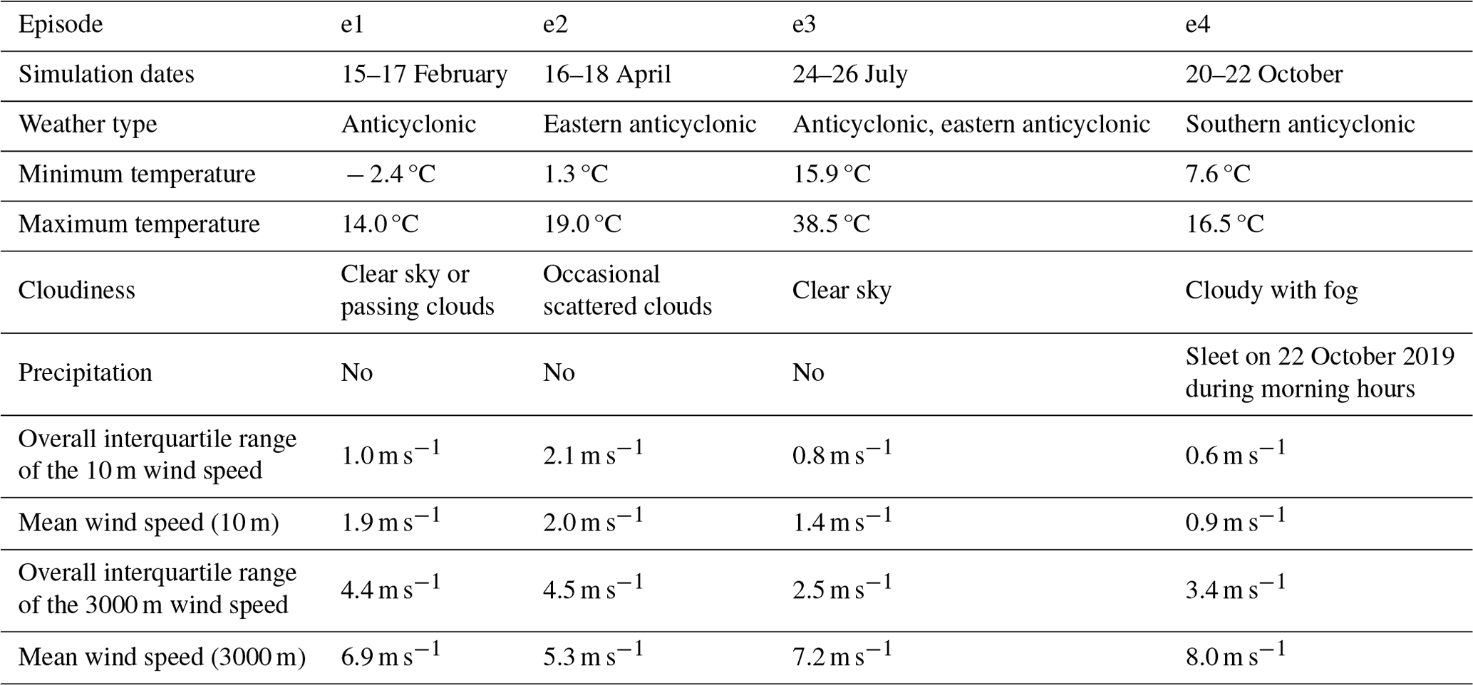
This experiment encompasses four different 72 h episodes in February, July, April, and October of 2019. Furthermore, only anticyclonic weather types are taken into consideration, since according to Zahradníček et al. (2022), these types were the most frequent ones that occurred in the Czech Republic during the 1961–2020 period. Additionally, specific weather events we take an interest in, i.e., bad air quality periods, heatwaves, and stable and calm weather, coincide with and are a consequence of these weather systems. For instance, during winter (December, January, and February), they are characterized by clear and bright skies, with light wind speeds or no winds at all. These conditions, especially during the evening and nighttime, often lead to the occurrence of temperature inversion, a condition favorable for trapping the pollutants from vehicles, heating, etc., creating bad air quality conditions within urban environments. Temperature inversion events are the strongest during winter but can be observed during the other three seasons as well. To give an example, the aforementioned phenomenon and bad air quality conditions within urban environments are used as an episode in a validation study by Resler et al. (2021). Similarly, in summer (June, July, August), when the sky is clear, the sun warms up the ground continuously, bringing hot and dry weather, which oftentimes, during anticyclonic conditions, leads to the creation of a weather event known as a heatwave (see, e.g., Belda et al., 2021; Resler et al., 2021). Besides the intolerable temperatures that heatwaves bring to city inhabitants, the occurrence of increased ground-level ozone concentrations in urban areas is another repercussion of this event (see, e.g., Resler et al., 2021). Thereby, we take an interest in these two extreme weather phenomena for several reasons. Firstly, both have serious implications for city dwellers' health and well-being. Secondly, heatwaves and bad air quality conditions are the two most important hazards for the city of Prague. And lastly, they are important for the PALM model’s future validation (see, e.g., Resler et al., 2017, 2021). Nonetheless, to broaden the study and to see if the model behaves consistently throughout the year, we included two other seasons (spring and autumn) without unique weather events. Hence, two more episodes have been selected, one in April and another in October. The choices of the simulation periods in 2019 are as follows: 15–17 February (e1), 16–18 April (e2), 24–26 July (e3), and 20–22 October (e4). For detailed information about the meteorological conditions during the selected episodes, see Table 1.

Table 1 Meteorological conditions during the selected simulation episodes.

2.2 PALM model configuration

2.2.1 Model description and configuration

Simulations were done by the PALM model (Maronga et al., 2020). The PALM model is based on the large-eddy simulation (LES) approach, and it solves non-hydrostatic, filtered, Boussinesq-approximated, incompressible Navier–Stokes equations. We selected the following configuration of the individual processes in the PALM model for our simulations. The subgrid stress tensor is modeled by the Deardorff (1980) 1.5-order closure involving Moeng and Wyngaard (1988) and Saiki et al. (2000) modifications. Pressure is calculated by a Poisson equation solved with the multi-grid scheme (description, e.g., in Maronga et al., 2020). For spatial and temporal discretizations, the upwind-biased fifth-order differencing scheme (Wicker and Skamarock, 2002) and the third-order Runge–Kutta time-stepping scheme (Williamson, 1980) are employed, respectively. This core system is complemented by the so-called PALM for urban application modules (PALM4U) specifically developed for studying the urban boundary layer and application to concrete problems, i.e., city planning, urban climate studies, etc. (Maronga et al., 2020). They include, e.g., a land surface model (LSM; Gehrke et al., 2021), a building surface model (BSM; Resler et al., 2017; Maronga et al., 2020), a radiative transfer model and plant canopy model (RTM and PCM; Krč et al., 2021), a human biometeorology module (BIO; Fröhlich and Matzarakis, 2020), online nesting (Hellsten et al., 2021), and mesoscale nesting (MESO; Kadasch et al., 2021). The modules employed in this experiment are LSM, BSM, RTM, BIO, and MESO.

For the purposes of the experiment, 14 simulations were conducted, and the length of each simulation episode was 72 h. Moreover, to adjust the temperatures of the individual elements of soil, building walls and roofs, and pavement layers, which are initialized from the coarse mesoscale simulation and prescribed by PALM configuration, our setup included a PALM-provided spin-up simulation for a period of 24 h. During the spin-up simulation, only simplified energy-related processes are simulated, while the dynamic part of the model's code is switched off (see details in Maronga et al., 2020). It allows the simulation to start with the temperature of surfaces and material below the surfaces partly adjusted to microscale conditions. These adjustments are not perfect due to the simplified nature and limited time of the spin-up run. For this reason, the results of the first hours of the actual simulation need to be interpreted with care, mainly in the case of near-surface processes, while in the case of profiles, the possible influence is minor.

2.2.2 Input data and domain configuration

To solve the energy-balance equations and radiation interactions, BSM, LSM, and RTM require the use of detailed and precise input parameters describing the surface materials, such as albedo, emissivity, roughness length, thermal conductivity, thermal capacity, and the capacity and thermal conductivity of the skin layer. Urban and land surfaces as well as subsurface materials become very heterogeneous in a real urban environment when a very fine spatial resolution is used. For this study, three different data sources were used as input: (i) the Copernicus Land Monitoring Service's Urban Atlas 2018, (ii) the OpenData platform of the Prague Municipality (digital elevation model, building heights, etc.), and (iii) OpenStreet Maps as a source of building locations outside of the city of Prague. All datasets were processed to the static driver, an input file needed for the PALM model initialization (see PALM Input Data Standard – PIDS in PALM model documentation).

The domain used in this experiment is located in the southeastern part of Prague (see Fig. 1). In the central, northern, and northwestern parts, the simulated domain is made up of diverse types of areas and includes all the typical objects that characterize an urban area (e.g., continuous and dense urban areas, transit roads, green urban areas, water bodies; Fig. 1). The northeastern part contains large green urban areas (code 1410 in Fig. 1). Moreover, the eastern and southern parts are made up of arable land. The Vltava River crosses the domain in the south–north direction in the western part. Such a land cover formation in the domain covers a diverse set of areas, chosen to challenge the model performance across the mentioned composition. Elevation in the domain varies between 171 and 381 m, and the mean elevation is 275 m. The highest hills are located in the southern parts of the domain. The Vltava River has formed a deep valley in the western part; one small valley is located in the center of the domain and a second larger one in the northern part, both of them forested. Slopes close to the valleys are steep and change continuously to a plateau (see Appendix F). In the horizontal direction, the domain has a dimension of 8×8 km with 10 m horizontal resolution. Vertically, it extends up to the height of 2830 m distributed on 162 vertical levels, and 10 m resolution is applied until 350 m height is reached, after which a stretching factor of 1.08 is implemented with a maximum stretching length of 20 m.

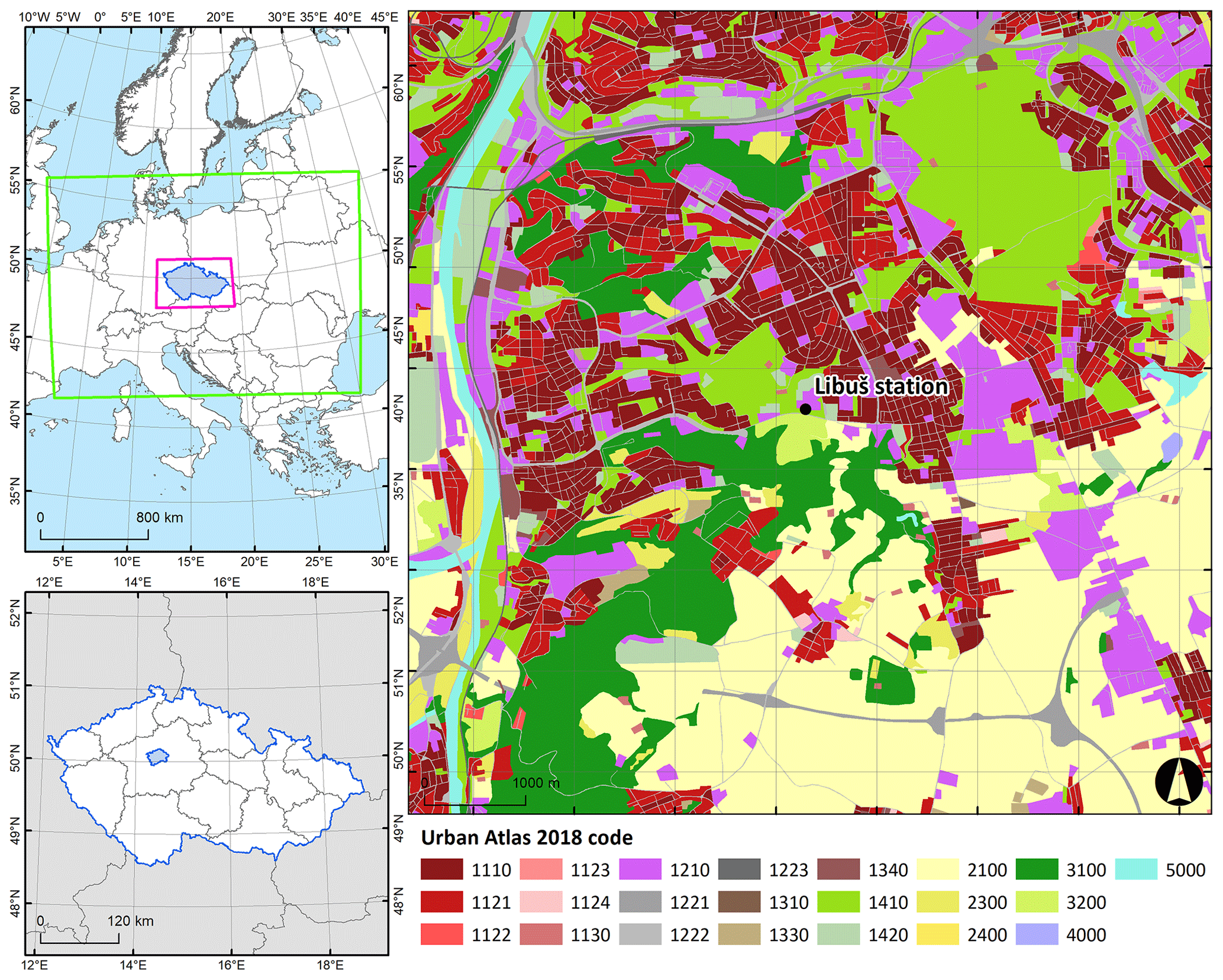
Figure 1 The location of the modeled domain in Europe (top left) and in the Czech Republic (bottom left). The WRF model's outer and inner domains are depicted at the top-left part of the figure with green and pink colors, respectively. The map of the domain within the city of Prague with the Libuš station (WMO ID 11520) location is presented on the right part of the figure. Land cover categories shown on the right are represented using the Urban Atlas 2018 geodatabase with respective codes described in Urban Atlas (2018).

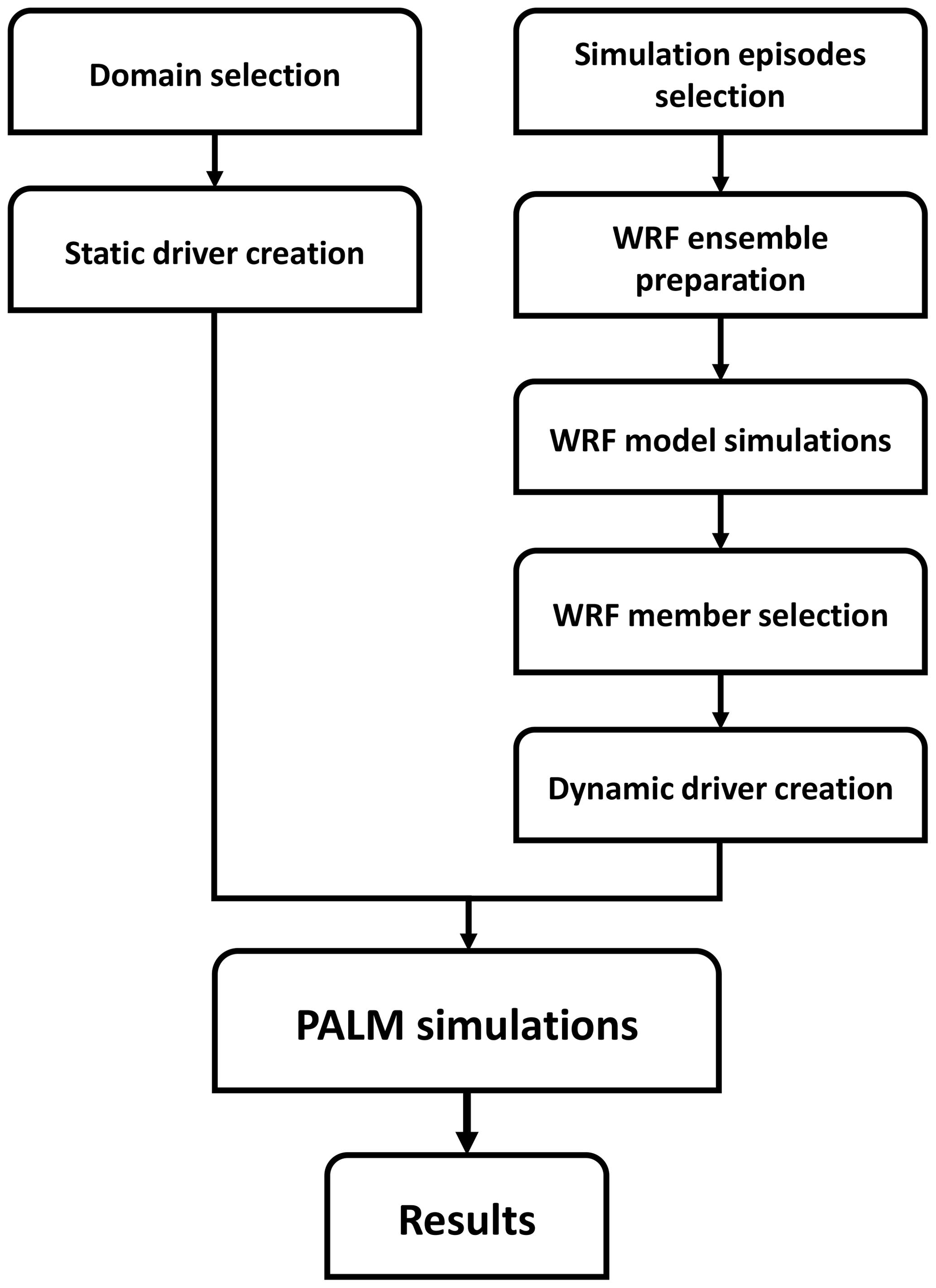
2.2.3 Initial and boundary conditions

The dynamic driver input file is used to supply the IBC for the PALM model. It consists of initial information for the entire domain and dynamic information about the time-dependent conditions at the boundaries. The 3D fields of the potential temperature, velocity components (u, v, w), and water vapor mixing ratio originated, e.g., from the WRF model are horizontally and vertically interpolated to the PALM model grid. Since the PALM model represents terrain in a higher resolution in comparison to the WRF model, the vertical interpolation process incorporates stretching such that the bottom-level fields follow the fine terrain while avoiding vertical distortion at the high levels.

The processing of WRF data starts with the coordinate system transformation between the WRF model projection (Lambert conformal conic with custom parameters) and the PALM grid projection (UTM) and bilinear horizontal interpolation of the 2D and 3D WRF fields while keeping the WRF vertical structure.

In the next step, the vertical interpolation of the 3D fields together with terrain matching and vertical stretching is linearly performed for each PALM grid column on the pressure coordinates, where the shifted pressure ${\stackrel{\mathrm{̃}}{p}}_{l_n}^{\mathrm{W}}$ of WRF level n is calculated as

$${\stackrel{\mathrm{̃}}{p}}_{l_n}^{\mathrm{W}}=\left\{\begin{array}{ll}\left(p_{l_n}^{\mathrm{W}}-p_{\mathrm{t}}\right)\frac{p_{\mathrm{s}}^{\mathrm{P}}-p_{\mathrm{t}}}{p_{\mathrm{s}}^{\mathrm{W}}-p_{\mathrm{t}}}+p_{\mathrm{t}},& \text{if }{p}_{l_n}^{\mathrm{W}}>p_{\mathrm{t}}\\ p_{l_n}^{\mathrm{W}},& \text{if }{p}_{l_n}^{\mathrm{W}}\le p_{\mathrm{t}},\end{array}\right.$$

where $p_{l_n}^{\mathrm{W}}$ is the original WRF level n pressure, $p_{\mathrm{s}}^{\mathrm{W}}$ is the WRF surface pressure, $p_{\mathrm{s}}^{\mathrm{P}}$ is the pressure corresponding to the PALM terrain, and p_t is the transition-level pressure (the upper stretching limit) that is taken from the average pressure 2000 m above the domain base. The boundary conditions are then taken from the interpolated 3D fields.

Finally, in order to ensure mass balancing on the boundaries, the total volumetric flow rate residue (inflow minus outflow) is calculated for each time step. This residue, divided by the total area of all five boundaries, is then subtracted from the inflow wind speed (which is positive on the inflow and negative on the outflow) such that the total flow rate residue of the updated wind field becomes 0. With the constant-density Boussinesq approximation used in PALM, balancing volume also balances mass.

Along with the atmospheric fields, the soil moisture and temperature and a time series of large-scale surface forcing of surface pressure are taken from WRF and provided to PALM. The data from WRF retain the original temporal resolution of 1 h as PALM performs temporal interpolation internally. Further guidance on data transformation and dynamic driver creation is available in Resler et al. (2021) and PIDS. The radiation variables, i.e., the downwelling shortwave (SW) and longwave (LW) radiative fluxes, were taken from the WRF model auxiliary outputs, which had an increased temporal resolution of 10 min.

In addition, one physical phenomenon not resolved by the mesoscale model is turbulence; thus it must be generated at inflow boundaries artificially. This process is managed by the PALM synthetic turbulence generator based on digital filtering of pseudo-random numbers (STG; Xie and Castro, 2008). Turbulence perturbations are forced into velocity components in the parent domain’s lateral boundaries at every time step according to prescribed values of the Reynolds stress tensor components and integral length scales. Their values are parameterized in PALM using empirical similarity theory profiles. All dynamic drivers used for this study were generated from the inner domain of the WRF model (Sect. 2.3).

2.3 WRF model configuration

The WRF mesoscale model (Skamarock et al., 2019) in version 4.4 was used to drive the PALM model through the PALM's mesoscale nesting system. The model was run on two nested domains at horizontal resolutions of 9 and 3 km. The extent of the domains is 225×180 and 187×121 grid cells for the outer and inner domains, respectively, with 49 vertical levels. For its initialization, ERA5 reanalysis was used. For the purposes of the experiment, an ensemble of 16 members was designed, with members differing in three factors (physics parameterizations) in which we expect an impact on the urban simulation. This design is “balanced” similarly to the statistical analysis of variance; i.e., every combination of factors is equally represented. Thus we have the following:

• two versions of the surface layer scheme (the MM5 Similarity Scheme (Paulson, 1970), members 01–08, vs. the Revised MM5 Scheme (Jiménez et al., 2012), members 09–16);

• two versions of planetary boundary layer (PBL) parameterization (Yonsei University (YSU) PBL scheme (Hong et al., 2006), members 01–04 and 09–13, vs. the BouLac scheme (Bougeault and Lacarrère, 1989), members 05–08 and 13–16);

• four versions of urban parameterization (no urban parameterization, a single-layer urban canopy model – SLUCM (Chen et al., 2011), building environment parameterization – BEP (Martilli et al., 2002), and BEP in combination with a building energy model (BEP+BEM; Salamanca and Martilli, 2010)). This factor rolls the fastest; i.e., there is no urban parameterization in members 01, 05, 09, 13, etc.

Other parameterizations were in accordance with their common and widely used settings; e.g., NOAH LSM (Tewari et al., 2004) was used for all members. The Thompson scheme (Thompson et al., 2008) was used for microphysics for all ensemble members except member 12 which required the WRF single-moment five-class scheme (Hong et al., 2004) due to compatibility issues. The WRF ensemble simulation was performed for four episodes, which amounts to 64 simulations all together. This design enables us to capture the eventual systematic effects of distinct parameterizations, and it serves as a proxy for a multi-model ensemble of numerical weather prediction (NWP) models thanks to its variability in model setup. For a summary of the experiment design, see Table A1.

2.4 BC selection workflow

Running a 72 h simulation of PALM driven by each of the WRF ensemble members (i.e., 64 PALM model high-resolution runs) would be computationally expensive. Therefore a strategy of preselecting WRF ensemble members was developed to keep the computational costs low while satisfactorily sampling the variability. We classified the WRF simulations according to their performance in the representation of potential temperature and wind speed, evaluated against soundings taken at the Libuš meteorological station (WMO ID 11520) every day at 00:00, 06:00, and 12:00 UTC. The mentioned variables, i.e., potential temperature and wind speed, were chosen due to the fact that they are directly relevant for the PALM model’s validation and are responsible for the development of atmospheric processes. The evaluation was based on the root mean square error (RMSE) and correlation coefficient (r; Appendix C; see Resler et al., 2021 and Radović et al., 2022). Two WRF ensemble members with the best and worst performance (closest to and farthest from the observations) were then preselected for the PALM runs. The performance, however, differs between variables (a similar issue was observed in Vogel et al., 2022, and Radović et al., 2022); i.e., the best statistical values that some members showed for potential temperature were not the best for the same member in the case of wind speed. Keeping this behavior in mind, the members with the lowest and highest RMSE values for temperature and another with the same characteristics but based on the wind speed were selected, and the strategy was repeated for every one of the four selected periods. If two model members have similar RMSE values, the correlation coefficient may serve as a supporting statistical metric. The preselected configurations (coded by member numbers) are summarized in Table B1. Some configurations have multiple occurrences.

To support this method of selection, a series of descriptive statistics were computed to assess the effects of factors represented by the PBL, surface layer, and urban physics. No systematic superiority of one parameterization over another was detected. The effects that were observed were the following:

• for the October episode, the BouLac PBL outperforms the Yonsei PBL

• for the February episode, the SLUCM is systematically the worst urban parameterization.

Since no single effect captured the differences in performance, we preferred the selection method described above.

2.5 PALM model near-surface output processing

The PALM model near-surface output methodology processing is applied to two fundamental meteorological variables: air temperature at 2 m and wind speed at 10 m. In addition, the aforementioned processing is applied to three additional variables: mean radiant temperature (MRT), physiological equivalent temperature (PET), and the Universal Thermal Climate Index (UTCI). The mean radiant temperature (MRT), according to Krč et al. (2021), is defined as “the temperature of an imaginary object for which that object would be in radiative equilibrium with its surroundings, which means that the absorbed irradiance would be equal to the emitted radiant exitance”. The physiological equivalent temperature (PET) is defined by Höppe (1999) as “the air temperature at which, in a typical indoor setting, the heat balance of the human body (work metabolism 80 W of light activity, added to basic metabolism; heat resistance of clothing 0.9 clo) is maintained with core and skin temperatures equal to those under the conditions being assessed”. Finally, as stated by Jendritzky et al. (2012), the Universal Thermal Climate Index (UTCI) is “the isothermal air temperature of the reference condition that would elicit in the same dynamic response (strain) of the physiological model”. The MRT is evaluated as a variable affecting human energy balance and thermal comfort; it is also used for the calculation of other thermal indices. The biometeorological indices UTCI and PET are more practical than air temperature for human-related analysis, helping to understand weather conditions’ impact on individual health and society. In addition, they are used for decision-making in various public sectors, urban planning, etc.

The processing of PALM's near-surface outputs is done as follows. First, the selection of the averaging periods is made to distinguish between parts of the day influenced by the solar input. Hence, four different times of the day are considered, i.e., morning (1 h before sunrise), solar noon (30 min before to 30 min after solar noon, referred to as noon in the figures), daytime (between sunrise and sunset), and nighttime (between sunset and sunrise). The selected hours are adjusted according to the season for which the simulation was performed and are displayed in the coordinated universal time (UTC) time standard. Regarding the simulation results, only the differences between the PALM members driven by the WRF members with the lowest (the best) and highest (the worst) RMSE values are shown. The basic statistics obtained for both WRF and PALM model outputs are shown in Appendix E. Each table demonstrates the spatial minimum, average, and maximum of 72 h averages for each variable, period, and selected member. It must be noted that the PALM model 2 m air potential temperature values used for calculation and shown in the following figures is estimated from the logarithmic interpolation due to the fact that the first prognostic grid point is placed at a height of 5 m (see PALM model documentation). The same principle for a horizontal component of the wind speed at 10 m is used, while the vertical component is calculated accurately for each grid point in the modeled domain. The WRF model air temperature and wind speed outputs used for the near-surface comparison are taken from the lowest level available in the model. The lowest-level WRF model outputs are used since they are utilized for the PALM model IBC creation.

3 Results

3.1 Vertical structure

In this section, we compare the potential temperature and wind speed vertical structure for both WRF and PALM models with radiosoundings. WRF vertical profiles are taken from the grid box closest to the Libuš station, while PALM vertical profiles are averaged over a 10×10 grid box area around the center of the domain. The PALM profiles are spatially averaged due to the fact that the WRF grid cell is significantly larger than the PALM grid cell. Comparison of the vertical profiles is performed at the times of radiosounding collection (00:00, 06:00, and 12:00 UTC).

Before diving into a detailed analysis of individual episodes, we present an overall view of the simulations in terms of errors with respect to the soundings. The input data for RMSE values were taken from the 10 min averaged PALM model files with no additional temporal averaging employed before their calculation. The PALM and WRF model RMSE values used for scatterplots are summarized RMSE values, and they include the information about the vertical profiles for the 72 h simulation period (each day at 00:00, 00:06, and 12:00) for the first 300 m of the atmosphere and are summarized in Fig. 2.

Every point representing a simulation is marked as the best or worst according to the WRF ensemble member selection in Table B1. Since member 12 is the worst in both criteria for e2 and member 14 is the worst in both criteria for e3, we obtain $\mathrm{4}+\mathrm{3}+\mathrm{3}+\mathrm{4}=\mathrm{14}$ simulations with 9 sounding times per simulation, resulting in 126 points or 63 pairs of best and worst points. Moreover, the criteria used for selection are distinguished by color, and all the best and worst pairs are connected. Thus we can identify the improvement/deterioration in the RMSE when going from WRF to PALM (distance to the dashed diagonal line) and the improvement/deterioration when changing the parameterization of WRF (the connected point). Since the majority of the points lie under the diagonal, we can argue that the detailed modeling of PALM mostly brings an improvement in the vertical profile covering the first 300 m of the atmosphere. The positive effect is more evident in cases where the error in the WRF simulation is large. It is also seen that the effect of selecting a less appropriate parameterization in WRF can have a large impact on the error. Nevertheless, a corrective behavior of the PALM simulation is evident even in these cases. On the other hand, if the error in the WRF simulation is relatively small, we cannot claim a systematic improvement in the vertical profile, brought on by the PALM simulation. Summary statistics for all members were also incorporated as Taylor diagrams. They show that most of the intra-ensemble variability comes from the driving WRF, while the PALM simulations deviate only slightly (see Fig. S37 in the Supplement).

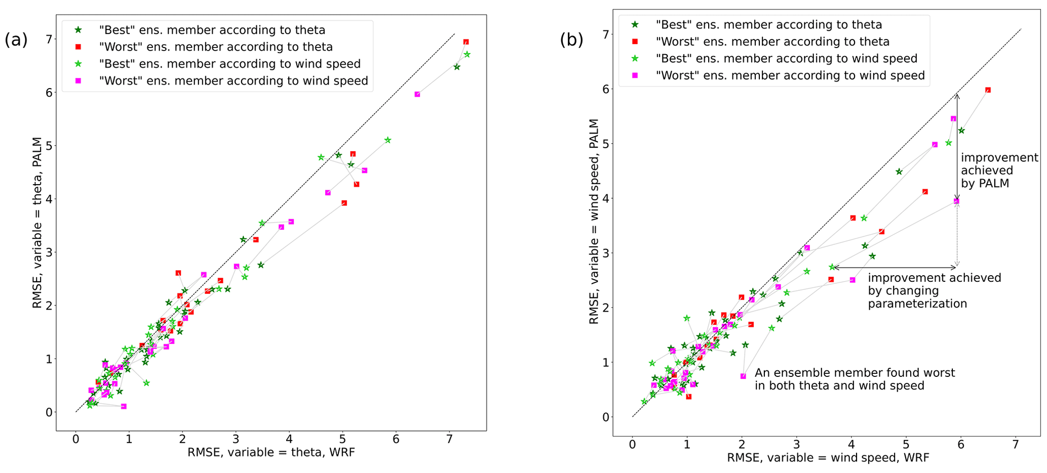
Figure 2 Scatterplots of PALM and WRF simulation RMSE values for potential temperature (a) and wind speed (b) vertical profiles for the first 300 m of the atmosphere and all preselected WRF model ensemble members, as well as for all PALM model simulations performed.

Next, we analyze the simulations in more detail for the two distinct seasons. The PALM model statistical metrics are calculated with respect to radiosoundings for the atmospheric layer of up to 3000 m a.s.l. (Appendix D). In the winter episode, during the night and morning, potential temperature vertical profiles from the PALM simulations do not deviate from the WRF-modeled profiles but are slightly warmer or colder than WRF profiles in the lower layers (Fig. S02a, c–d, f–g, and i). During the midday sounding hour, the PALM profiles follow the WRF profiles closely in both lower and higher atmospheric layers (Figs. S01–S02beh). In some cases, PALM simulations show added value over their driving conditions from WRF and are thus closer to the observations (e.g., Fig. S02c–d). Overall, the shape of the WRF potential temperature profile is captured by the PALM model. The atmospheric stability and instability are represented well by PALM. The PALM wind speed vertical profiles, in general, follow the WRF-modeled vertical profiles (Figs. S03–S04) but in some cases can deviate from them in the layers near the surface during morning and midnight hours (e.g., Fig. S04c–d and i). On the other hand, during the 12:00 UTC times, the agreement between PALM and WRF is much larger in the layers close to the surface. Altogether, compared to the potential temperature, wind speed vertical profiles show larger discrepancies between WRF and PALM. The differences between the best (03) and the worst (02) WRF ensemble members' potential temperature vertical profiles are the most pronounced during the 12:00 UTC sounding hours (Fig. S02beh). On the other hand, the differences between the best (16) and the worst (10) WRF members’ wind speed vertical profiles are more pronounced across all sounding times (Fig. S04). The statistical analysis for the profile up to 3000 m a.s.l. shows that the PALM simulations with respect to the WRF model potential temperature have a lower RMSE in the case of member 03 and a higher RMSE for the rest of the members. In the case of the wind speed, the PALM model RMSE values are higher than all of their corresponding WRF ensemble members' (Tables C1 and D1).

In the summer episode, potential temperature vertical profiles from the PALM model are consistent with the respective WRF profiles and show the highest consistency during 12:00 UTC (see Figs. S09–S10beh). As in e1, the PALM model shows the added value over the WRF driving conditions, which is seen for member 12 (Fig. S10h–i). The shape of the PALM profiles follows the WRF profiles, but smaller discrepancies can be seen in the lower atmospheric layers. The atmospheric stability and instability are captured well by the PALM model during all but one sounding time (see Fig. S10g). Similarly to the wind speed profiles in e1, in this episode, the PALM profiles generally stay consistent with the WRF profiles, but the largest discrepancies can be seen during the nighttime sounding hours (Fig. S12cfi). The differences between the best (01) and worst (12) WRF simulations are not pronounced in the potential temperature profiles (Fig. S06). In the case of the WRF wind speed profiles, the differences between the best (07) and the worst (12) members are more noticeable (Fig. S08). The RMSE values calculated for the PALM potential temperature profiles for e3 are lower in comparison to their WRF member pairs' RMSE values. On the other hand, for the same episode, the RMSE calculated for the wind speed profiles is higher for the PALM members (Tables C3 and D3).

In summary, the highest consistency between the PALM models’ vertical profiles and the corresponding WRF model profiles is seen during 12:00 UTC, and this behavior is valid for all simulation episodes. In general, the shape of the WRF profile is followed by the PALM profile, and most of the differences between the PALM and WRF vertical profiles are seen in the layers near the surface. In certain cases, the PALM model introduces an added value to driving WRF conditions (see Fig. S10b and h–i). The wind speed vertical profile comparison is more chaotic, and depending on the simulation period and the sounding time, the correspondence between the PALM model and the WRF's profiles can vary. In general, the differences between them are the highest in the layers closest to the surface, which is to be expected since the terrain representation is different in these two models. This behavior has already been seen in the work done by Resler et al. (2021). The statistical analysis performed on the PALM vertical profiles showed that in the case of e1, e3, and e4, RMSE values obtained for the wind speed are higher for PALM than for WRF, while for e2, they are lower. The PALM RMSE values for the potential temperature vertical profiles are lower than the WRF RMSE values in the case of e2, e3, and e4, and for the three (02, 10, 16) members they are higher for the PALM model in e1. This analysis has a limiting factor which is related to having radiosounding observations only three times per day, thus preventing us from performing more robust statistical and qualitative analysis.

One aspect exhibited by PALM and worth pointing out is related to its ability and inability to capture nighttime atmospheric stability. During the midnight sounding times, atmospheric stability is periodically captured by the PALM model. It can be seen that PALM, in some instances, does improve the driving data and brings the profile closer to the observed one by capturing nighttime stability (see Figs. S10i, S12f, and S14if). Yet, this behavior is not consistent, and, for example, in Figs. S06cf and 10cf we do not see such an effect; i.e., the WRF model fails to capture the nighttime stability, but PALM does not introduce any improvement in the driving profiles and fails to produce cooling. We attribute this behavior to the PALM model's dynamic core, but more experiments are necessary to fully understand this issue.

3.2 Near-surface evaluation

The second set of results refers to the influence of the selected pairs of BCs on temperature at 2 m and wind speed at 10 m. For the July episode, MRT, PET, and UTCI indexes were also computed. The figures depict the best and worst difference for the two WRF members and the difference for the corresponding PALM members driven by them. For each daytime period we display the WRF field and the corresponding PALM field. The WRF model grid boxes, in which the majority of land use is of an urban type, are outlined in black. Conversely, the majority of the grid box area is not of an urban type, although some of it can be. Note that the PALM domain is represented by a red square in the WRF field, and the figure thus illustrates the downscaling of a couple of WRF grid points to a much higher resolution and, in particular, the amplification or attenuation of BC differences by the downscaling process executed by PALM. In the text, the results for February and July are presented. The results for the other two episodes are deferred to the Supplement. The best and worst classification is based on potential temperature.

In Fig. 3, differences in the air temperature between members 03 and 02 for the February episode and four different averaging periods (morning, noon, daytime, nighttime) are presented. For all periods we can see a qualitative consistency between the WRF grid point values and PALM fields. The downscaling process done by PALM exhibits a distinct suppressive behavior, which can be attributed to the fact that both sets of BCs undergo the same local processes. On the other hand, the added value brought by the LES model, in particular by the high-resolution topography, surface representation, and resolved turbulence, is clearly seen. The local processes naturally enlarge the differences within the fields, and these differences are often “transported” to different locations compared to the WRF field. Also, note the fringe-like pattern in Fig. 3a, with both positive (0.5 to 2 K) and negative (−0.5 to −2 K) differences appearing across the domain. The same effect is seen in Fig. 3f, although it is less pronounced. This may be attributed to different urban parameterizations in the WRF members. In addition, rough transitions in the driving fields may promote the generation of waves in the microscale model. The argumentation above is supported by the descriptive statistics in Table 2, where we can see lower average differences in the PALM fields but mostly higher minimum and maximum differences.

Table 2 February episode minimum (min), average (avg), and maximum (max) differences in air temperature for four different averaging periods (morning, noon, daytime, and nighttime) between members 03 and 02 for the WRF and PALM models. For PALM fields, the differences in the air temperature at 2 m are taken from the 2D 10 min averaged files, while for WRF fields the air temperature from the lowest model level was taken.

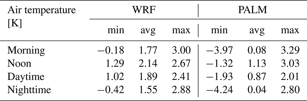
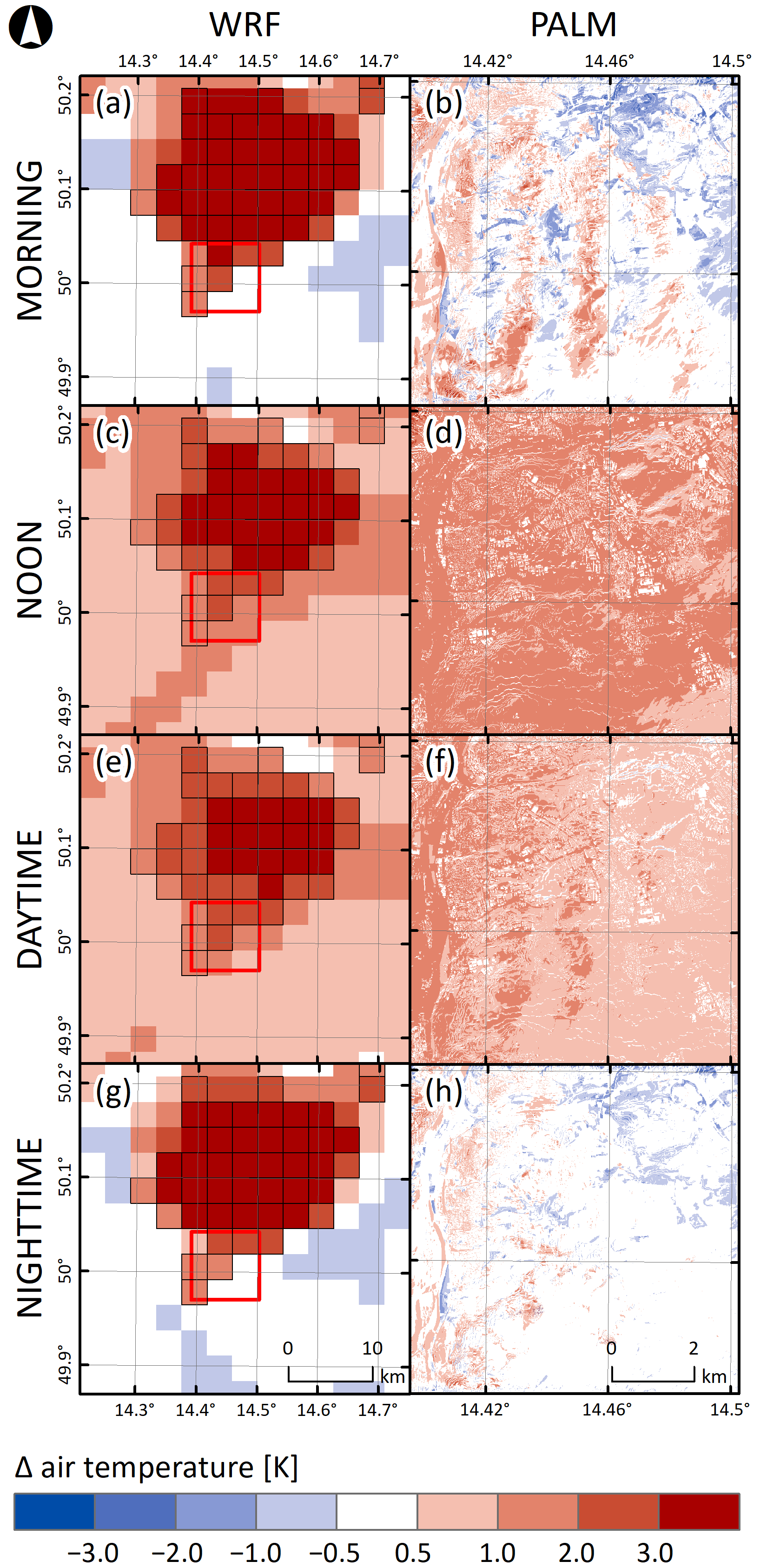
Figure 3 Differences between 72 h averages of air temperature for four selected periods (morning, noon, daytime, and nighttime) taken from WRF and PALM model members 03 and 02 for the February episode. The first column refers to the difference between the best (03) and the worst (02) WRF model members selected based on the potential temperature, and the second column refers to the difference between the PALM model members driven by the said WRF model members. The PALM model simulation domain is depicted with the red square. The WRF model grid boxes, in which the majority of land use is of an urban type, are outlined in black.

Differences in the air temperature for four different averaging periods (morning, noon, daytime, and nighttime) during the July simulation episode between members 01 and 12 for the WRF model and the PALM model are shown in Fig. 4. The overall behavior of the downscaling process shows similar effects to the February episode. This is also confirmed by the values in Table 3. The influence of the orography and land use on the differences is more evident compared to the February episode. One noteworthy feature is that in the summer episode, the differences between the two WRF simulations are on average more pronounced during the night, while in February, nighttime differences are higher. Exploring this behavior is beyond the scope of this paper; however, in terms of the influence on the high-resolution simulation, PALM follows this behavior.

For both February and July episodes, it is clear that the differences in the WRF fields are the largest in the urban area. Since all four members share the YSU parameterization of PBL, the differences have to be attributed to urban parameterization, which is 0 vs. BEM in the July episode and BEP vs. UCM in the February episode (see Table A1). These differences in the WRF fields thus propagate into the microscale simulation.

Table 3 July episode minimum (min), average (avg), and maximum (max) differences in air temperature for four different averaging periods (morning, noon, daytime, and nighttime) between members 01 and 12 for the WRF and PALM models.

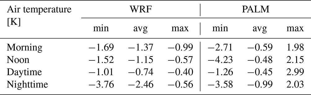
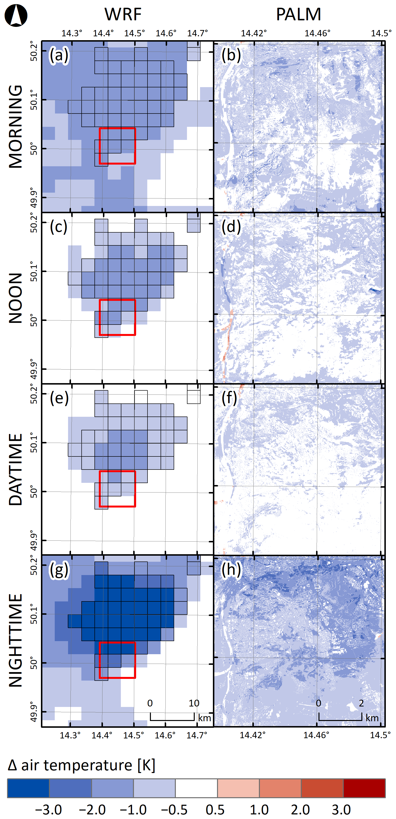
Figure 4 Differences between 72 h averages of air temperature for four selected periods (morning, noon, daytime, and nighttime) taken from WRF and PALM model members 01 and 12 for the July episode. The first column refers to the difference between the best (01) and the worst (12) WRF model members selected based on the potential temperature, and the second column refers to the difference between the PALM model members driven by the said WRF model members. The PALM model simulation domain is depicted with the red square. The WRF model grid boxes, in which the majority of land use is of an urban type, are outlined in black.

For convenience, we provide a detailed view of one of the maps together with the land use in Fig. 5. The PALM output in Fig. 5b for the nighttime averaging period is taken from the 07–12 pair chosen based on the statistical analysis of the wind speed. This comparison shows that the differences between the two simulations at the local scale are driven mainly by the difference in land use, and thus the full difference is a composite of large-scale and local-scale forcings.

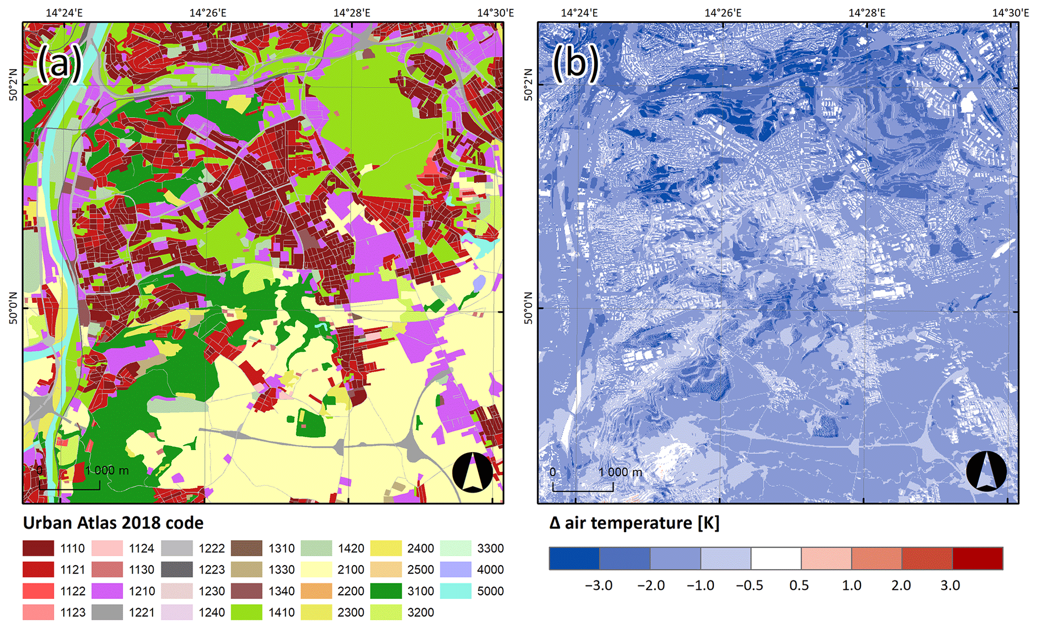
Figure 5 Differences between 72 h averages of air temperature for the July nighttime period simulated by PALM model members 07 and 12 (b) and land use (a).

From the results of the two episodes, we can conclude that the PALM differences are altogether analogous to the WRF differences as seen for example in the case of e3 for all averaging periods (Fig. 4). The same conclusion applies for e1 in the case of noon and daytime averaging periods (Fig. 3c–f). However, for the morning and nighttime period for e1, PALM introduces negative differences, ranging from 0 to −1 K, which are especially visible during the morning averaging time. For both presented episodes, PALM differences are on average lower and attenuated in comparison to the corresponding WRF differences. Moreover, the average differences for all averaging times are lower for PALM, especially during the morning and the nighttime averaging periods for e1 where they have values of 0.08 and 0.04 K, respectively, which means that PALM, in general, does not amplify the differences across the domain (see Tables 2–3). With respect to the wind speed, the attenuation of the differences is more pronounced, especially during the daytime and noon averaging periods across all simulation episodes (see, e.g., Figs. S19, S23, S27, S31). The PALM differences are consistent with the given driving field, i.e., if one WRF ensemble member is warmer or colder, the same member will be warmer or colder in the PALM model as well. On average, PALM tends to diminish the differences (Figs. 4f and S21c–g), but it does take over and amplifies them on certain surfaces such as water bodies (see Fig. 1, surface code 5000), where a certain nonlinearity in the response exists, and PALM creates its own structures (see also, e.g., Figs. 4d and S25cdf).

To provide a summary of the PALM model's sensitivity to the BCs, an additional analysis was performed in which the spatially averaged 1 h average differences in air temperature and wind speed were analyzed between all the PALM outputs. The analysis is presented for e1 and e3 in Figs. 6–7, respectively, while the rest of the analysis is included in the Supplement as Figs. S35–S36.

As for the time period of the PALM differences themselves (b, d, f, h in Figs. 3–4), a time pattern may occur. In the case of e1 (Fig. 6), the average differences show a diurnal cycle. This pattern is more prominent in the case of air temperature (Fig. 6a) where differences start to increase around 06:00 UTC until approximately 14:00 UTC. On the other hand, the average differences calculated for the wind speed are low most of the time and start increasing only at the end of the second day of the simulation. This diurnal pattern is present for e3 as well, with slightly larger magnitudes of differences than in e1 (Fig. 7). The average differences have a shorter period of increase lasting from 17:00–00:00 UTC for both air temperature and wind speed (Fig. 7).

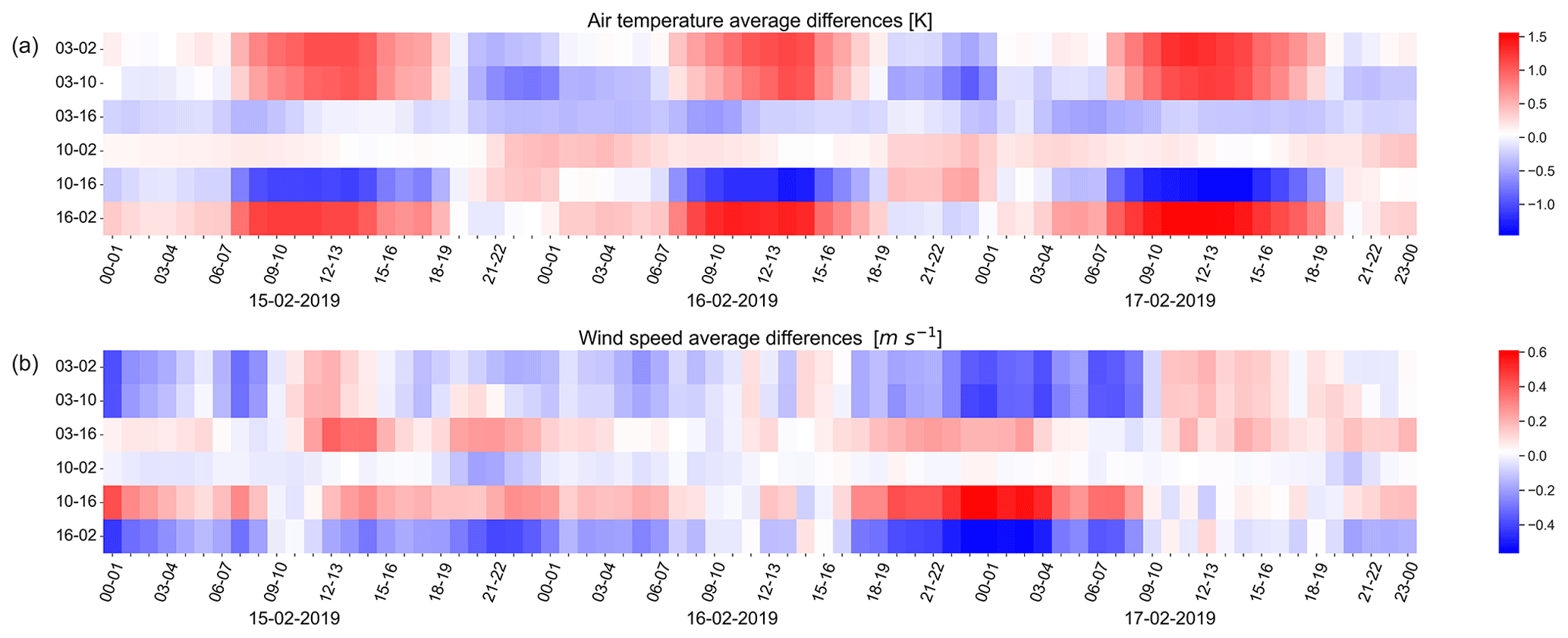
Figure 6 Spatially averaged 1 h average differences in air temperature (a) and wind speed (b) calculated for all the combinations taken from the PALM model outputs for e1. On the x axis, the averaging hours in UTC along with the simulation dates are presented, and on the y axis are the ID numbers of the PALM model differences.

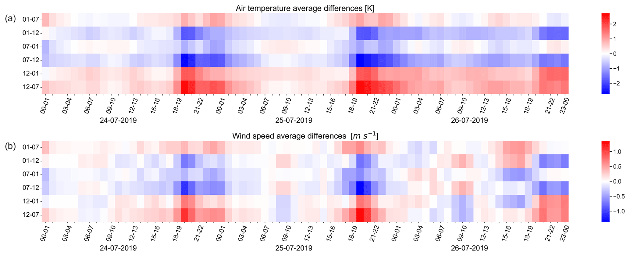
Figure 7 Spatially averaged 1 h average differences in air temperature (a) and wind speed (b) calculated for all the combinations taken from the PALM model outputs for e3. On the x axis, the averaging hours in UTC along with the simulation dates are presented, and on the y axis are the ID numbers of the PALM model differences.

It is apparent from Figs. 6–7 that during certain hours, differences between two PALM simulations driven by a different set of BCs are relatively small. This further means that the effect of the BCs is not large during this time and that the local processes resolved by the high-resolution PALM model are able to suppress their influence.

3.3 Influence of the BCs on the biometeorological indexes during e3

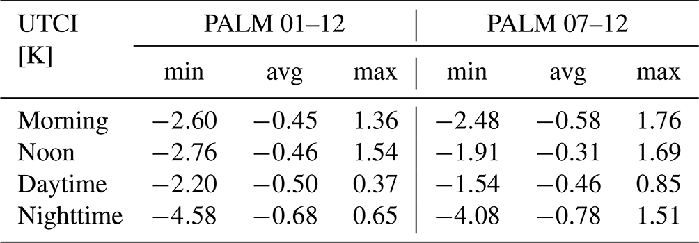
The PALM model has been proven to be of service for urban planning and the UHI mitigation strategies (e.g., Belda et al., 2021), and it is for example applied in the works of Geletič et al. (2022, 2023) for heat stress mitigation strategies. One of the major conclusions of Belda et al. (2021) was that PALM can show opposite sensitivity between physical and biophysical temperature indicators. The differences in the UTCI index obtained from the PALM model members for e3 (Fig. 8) show a consistent response in temperature and UTCI. The strongest minimum average difference has the 01–12 pair for the nighttime averaging period (−4.6 K), and the strongest differences are present near the northern and western boundaries of the simulation domain. The highest maximum average difference for the noon averaging period is 1.5 K. The average difference for all four periods is around −0.5 K. The 07–12 pair shows similar behavior for the nighttime (−4.1 K) but with more significant effects of elevation differences predominantly visible close to deep valleys (see Appendix F). The highest maximum average difference was found for the morning averaging period (1.8 K). The average differences obtained for UTCI do not differ much from the averaged values obtained for the air temperature (Tables 3 and E5); this behavior is valid for both pairs (see Table 4).

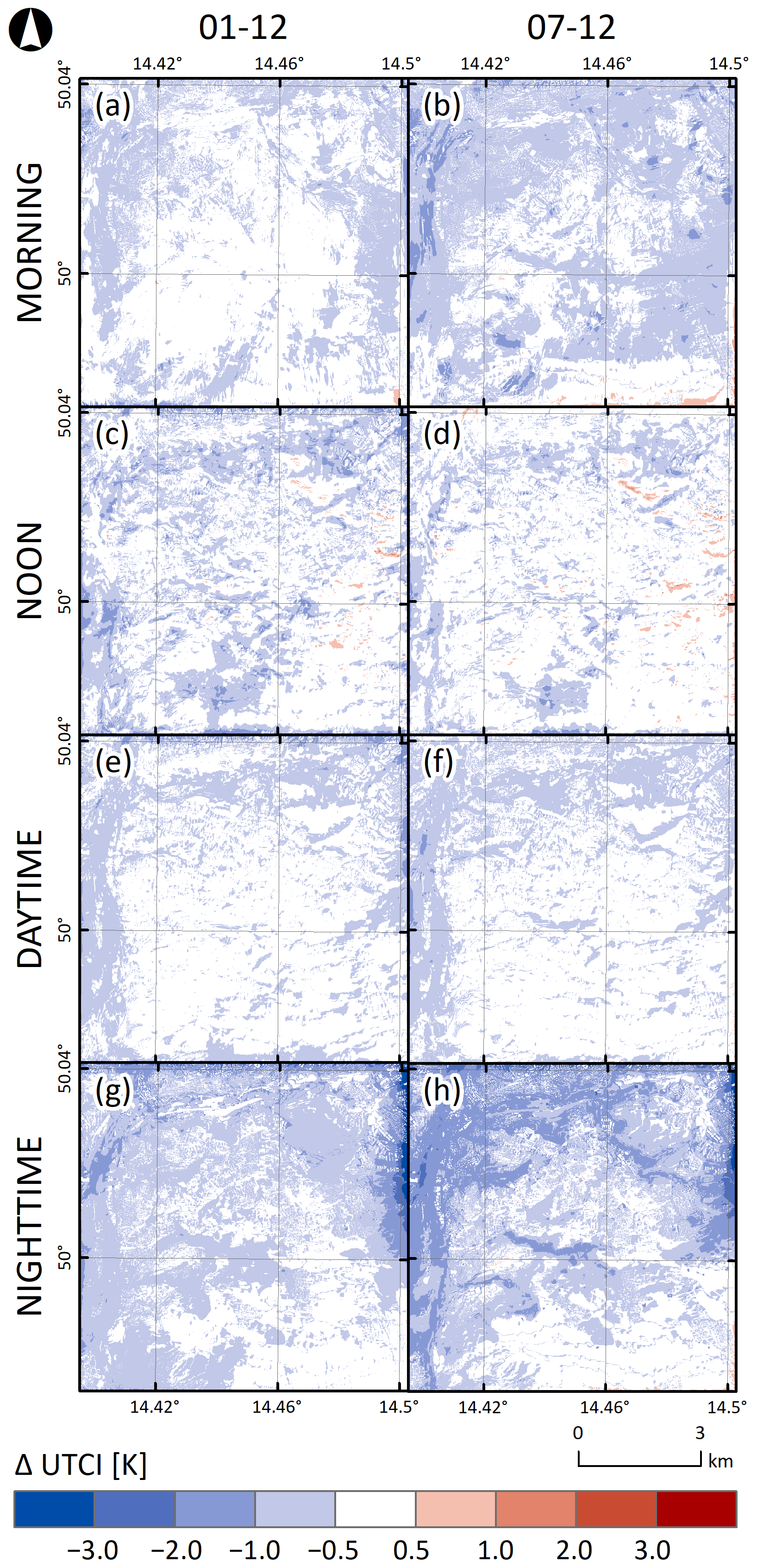
Figure 8 Differences between 72 h averages of UTCI for four selected periods (morning, noon, daytime, and nighttime) taken from the PALM model simulations for the July episode. The first column refers to the difference between the best and the worst member selected based on the potential temperature (01–12), and the second column refers to the difference between the best and the worst member selected based on the wind speed (07–12).

Table 4 July episode minimum (min), average (avg), and maximum (max) differences in UTCI for four different averaging periods (morning, noon, daytime, and nighttime) between members 01 and 12 and members 07 and 12 for the PALM model.

4 Discussion and future aspects

Resler et al. (2021) showed that in order for a PALM simulation to be realistic, good quality of input data (static driver data, mesoscale forcing, etc.) is necessary. Their study also indicates that the errors occurring in the mesoscale model propagate into the PALM simulation. Thus a question is raised, namely, to what extent the driving conditions could be the main cause of potential errors and inconsistencies in the PALM model outputs.

Our validation of the vertical profiles confirms the importance of the driving conditions. For potential temperature, PALM profiles have, in general, a lower RMSE than the driving WRF ensemble members (e1 – member 03, e2, e3) or a similar RMSE (e1 – WRF member 02, e4); see Appendix D. On the other hand, the PALM RMSE values obtained for wind speed are higher (e1, e2 – WRF member 09, e3, e4) or similar (e2 – member 14).

Among the members of the ensemble of 16 different WRF model realizations differing in urban parameterization, PBL parameterization, and surface layer parameterization (Table A1), no specific setting can be marked as uniformly better than the rest, not even for any specific season. From a theoretical standpoint, all combinations are acceptable. If we base the comparison on the statistical metrics for one variable (e.g., potential temperature or wind speed), the results are not consistent across seasons. For a specific season, the selection of the best and worst ensemble member gives different results when based on potential temperature or wind speed. Some degree of inferiority is seen in member 14 (BouLac PBL, UCM urban par.) though, which in three out of the eight cases has the worst RMSE value, namely, for seasons e2 and e4 in potential temperature and in season e2 in wind speed (Table B1). In e2 it has the highest RMSE for both variables. Therefore, in order to determine whether the WRF model or a specific WRF model realization performs better or worse for a certain season and a certain variable, and whether it shows any kind of long-term consistency in general, an exhaustive long-term analysis has to be performed in advance.

The study of Belda et al. (2021) tested the sensitivity of the PALM model to potential erroneous material parameter settings in which they showed that the PALM model temperature shows the highest sensitivity of ±0.18 K to the setup of certain building and material parameters (e.g., albedo, emissivity). Compared to the mentioned study, the variability in response to near-surface temperature introduced by different driving conditions shown in this study is much higher than the variability coming from the surface parameters (±3 K), thus proving the PALM model's high sensitivity to BCs. However, tiles over dense urban areas appear less affected than tiles with natural surfaces, likely due to the added “forcing” of the urban surfaces, which can override the difference in the boundary conditions.

The WRF model used in this study is not able to explicitly resolve the large eddies that have a strong impact on the atmospheric flows, momentum, heat, and air pollution transport in the boundary layer, while on the other hand, the PALM model can. But, despite the assets of the PALM model, its results are largely dependent on the quality of the mesoscale WRF simulation. This is a principle usually known as “garbage in, garbage out” in many fields, such as limited-area regional modeling, in which the regional models cannot correct large-scale errors imposed from the lower-resolution driving models (e.g., Giorgi, 2019). An integral future perspective of this work is related to the coupling of the PALM model with more mesoscale models, namely, ICON, the ALADIN model, etc., and validating the mesoscale–microscale model couple against the observational data. Such experiments would help in the practical applications of mesoscale–microscale nested models. In situations when multiple mesoscale models are available for driving the microscale LES model, the information about the quality of their outputs would help to minimize uncertainty coming from the BCs, especially in the case of validation studies.

5 Study limitations

The work presented here, the PALM model configuration, and input data used have certain limitations, which are listed in the following paragraphs:

• The PALM model simulations are conducted only for specific 72 h periods. The main reason is that PALM simulations are computationally expensive. These 72 h periods, even though conducted for four episodes throughout the year, might not be sufficient to assess the full influence of the WRF model boundary conditions on the PALM model response and its results.

• Due to the prevailing anticyclonic weather type typical of the city of Prague and the Czech Republic in general, this study is limited to the aforementioned weather type. The sensitivity of the microscale model to the potential erroneous representation of synoptic-scale forcings, broader atmospheric conditions, mesoscale circulations, or rapidly moving weather systems such as fronts in the NWP model WRF has not been assessed.

• The resolution used for the simulations is 10 m, and no nested domain in higher resolution (e.g., 2 m) is utilized. Such choice of resolution can potentially mask certain phenomena and thus influence the assessment of the influence of the boundary conditions on the PALM outputs. Moreover, one cannot see how the higher-resolution domain would behave with respect to the driving conditions or if it would modify the driving fields in any aspect.

• This study does not investigate the influence of initial conditions separately but analyzes the joint effect of initial and boundary conditions. To separate the effect of initial conditions, additional tests would be needed.

• The sensitivity tests on the domain size and the grid box size have not been performed in this study.

• Due to the technical error during the process of static driver generation, there is a mismatch between the realistic terrain height and the terrain height used in the simulations. Thus the simulation terrain height is shifted down by 10 m with respect to sea level. To be sure that this shift does not affect the results, the e1 simulations were repeated. No substantial differences were observed, qualitatively or quantitatively.

• For the purpose of this study, we only used a particular sample of the WRF model outputs, thus not utilizing the full ensemble of the produced outputs due to the extremely high computational costs of the LES-based PALM model simulations.

• The WRF model in version 4.4 utilized for this study uses the Moderate Resolution Imaging Spectroradiometer (MODIS) dataset. However, Demuzere et al. (2023) recently developed and implemented a hybrid 100 m global land cover dataset for the WRF model based on local climate zone classification (Stewart and Oke, 2012). Such advancement in the resolution of a land cover can be important for urban modeling applications and can consequently change the behavior of the initial and boundary conditions produced by the WRF mesoscale model, further influencing the PALM model outputs.

• This study is a case study performed for the city of Prague, Czech Republic. In order to confirm the behavior and influence of the boundary conditions on the PALM model simulations, more case studies are necessary. Regardless, these results are applicable to the PALM model performance with regard to the BCs in general.

• Another limitation is related to the vertical profile comparison with the radiosoundings. Namely, the radiosoundings from the Libuš meteorological station are assimilated into ERA5 data used for driving the WRF model, thus influencing the comparison and introducing the bias into the evaluation of the correctness of the ensemble members. On the other hand, after many statistical analyses were performed, no member significantly outperforms the rest of the ensemble with respect to correctness or performance in relation to the radiosounding data. Moreover, the majority of the mesoscale models that could be potentially used for the preparation of the BCs for PALM have radiosoundings assimilated directly or indirectly as the WRF model through the ERA5 or other types of driving data, making it a general problem for these types of studies.

Considering all listed limitations, we recognize this study to be reliable with plausible results. The plausibility of the results is confirmed by the vertical comparison with the radiosounding observations.

6 Conclusions

The objective of this study was to address the following topics: (i) constructing a “perfect” set of BCs for the PALM model, (ii) assessing the sensitivity of the PALM model to the given BC set, and (iii) evaluating the performance of the PALM model based on the given BC set:

• i.

  The process of the construction of a perfect set of BCs from the WRF model for the purpose of driving the PALM model proved to be challenging. The evaluation of WRF outputs against observations has confirmed that the performance of any particular setting (e.g., parameterizations) differs among variables; often there is a trade-off between performance in one variable against another one, e.g., temperature and wind speed. Also, the performance may change with the season.

• ii.

  The differences between PALM simulations driven by different BCs decrease and increase periodically throughout the simulation time, and the time patterns are different for different seasons. This behavior is, to some extent, consistent between different pairs of the PALM model outputs (driven by different BCs), and it depends on the period of the day during the simulation time.

• iii.

  As a general rule, the PALM simulation conforms to the given set of BCs and shows substantial consistency with them. Thus the largest part of errors may indeed originate in the mesoscale model. The PALM model's performance, however, does not deteriorate when the given BC set is farther from the real state of the atmosphere (i.e., observations), and it does not lag when the BCs are close to the observations. As seen from this experiment, there is considerable potential for introducing erroneous information into PALM through the boundary conditions.

In order to fully assess the influence of the boundary conditions and PALM’s sensitivity to them, there is a need for long-term simulations followed by statistical evaluation, for different periods throughout the year. While being aware of the departures from reality introduced by the BCs, we may claim that PALM tends to attenuate the influence of possibly misspecified boundary conditions, and its response to differences in the boundary conditions is fairly robust. Also, PALM has the capacity to better reflect the local processes (e.g., surface interactions and generation of turbulence), which is clearly an asset in the field of high-resolution modeling of the urban areas. These facts support better confidence in the results of PALM simulations performed with the aim of comparing scenarios of urban development or mitigation strategies.

Appendix A: Summary of the experiment design – parameterizations in the WRF model ensemble members

Table A1 Summary of the experiment design – parameterizations in the WRF model ensemble members.

Appendix B: The WRF ensemble member ID numbers selected for each simulation episode

Table B1 The WRF ensemble member ID numbers selected for each simulation episode.

Appendix C: WRF ensemble statistical analysis of the potential temperature and wind speed vertical profiles up to the height of 3000 m a.s.l.: root mean square error – RMSE, correlation coefficient – r

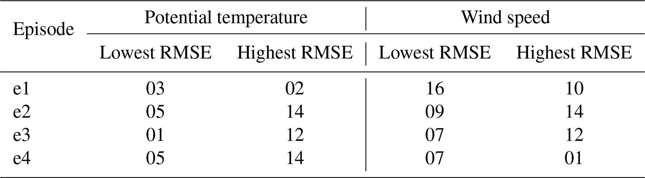
Table C1 February episode WRF ensemble statistical analysis of the potential temperature and wind speed vertical profiles up to the height of 3000 m a.s.l.: root mean square error – RMSE, correlation coefficient – r.

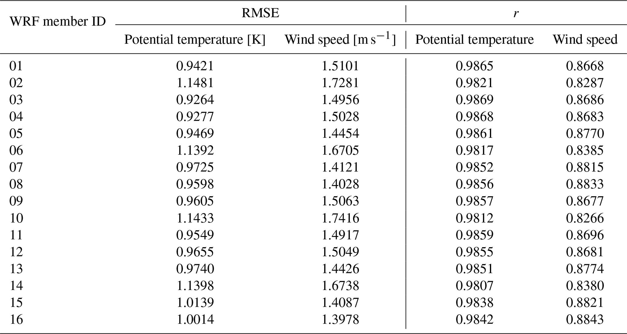
Table C2 April episode WRF ensemble statistical analysis of the potential temperature and wind speed vertical profiles up to the height of 3000 m a.s.l.: root mean square error – RMSE, correlation coefficient – r.

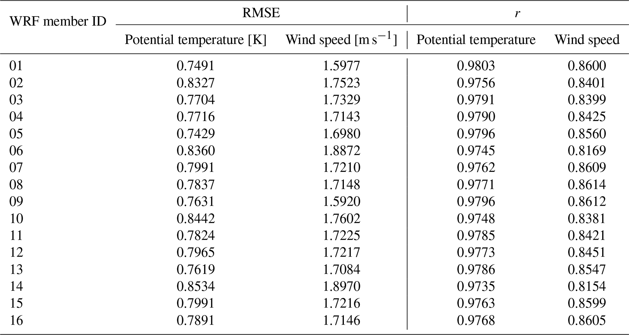
Table C3 July episode WRF ensemble statistical analysis of the potential temperature and wind speed vertical profiles up to the height of 3000 m a.s.l.: root mean square error – RMSE, correlation coefficient – r.

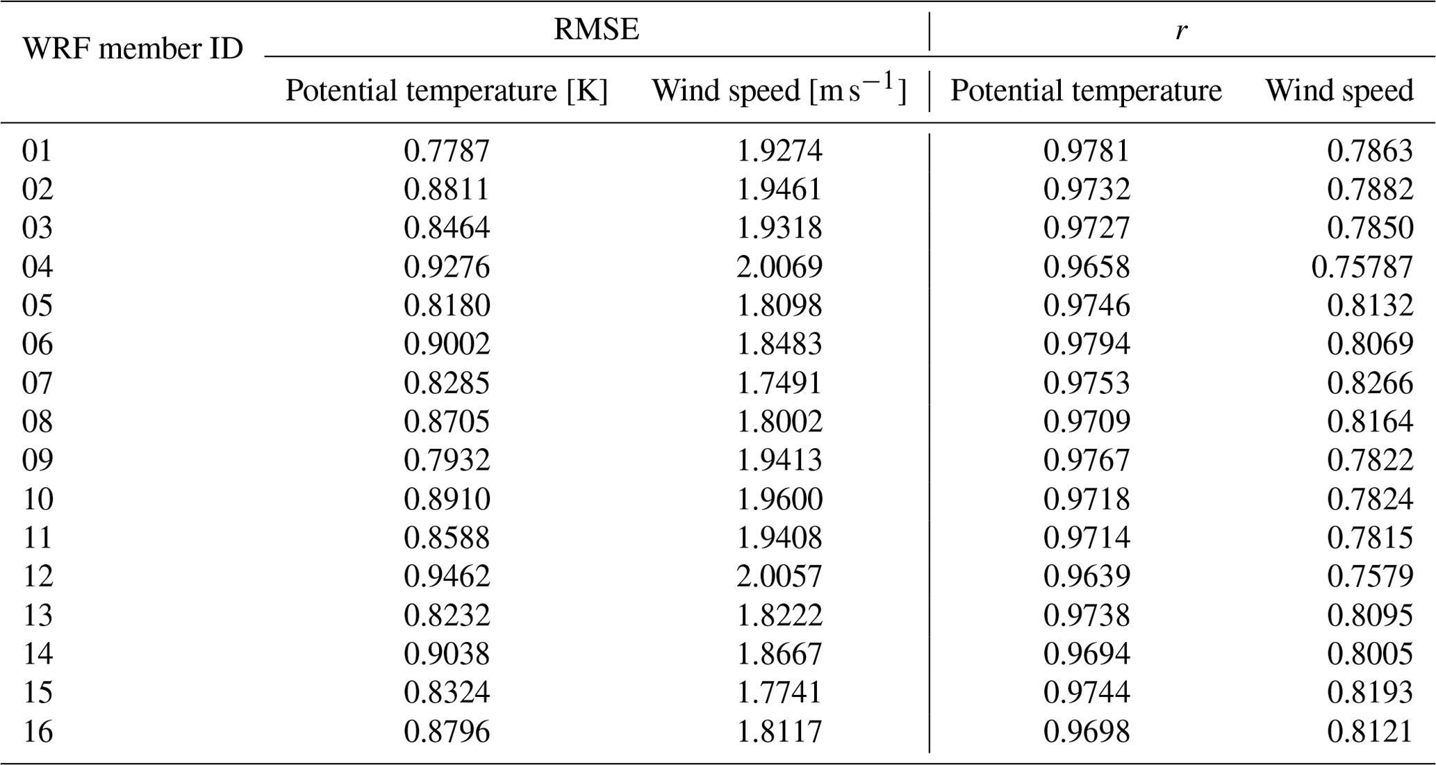
Table C4 October episode WRF ensemble statistical analysis of the potential temperature and wind speed vertical profiles up to the height of 3000 m a.s.l.: root mean square error – RMSE, correlation coefficient – r.

Appendix D: PALM ensemble statistical analysis of the potential temperature and wind speed vertical profiles up to the height of 3000 m a.s.l.: root mean square error – RMSE, correlation coefficient – r

Table D1 February episode PALM ensemble statistical analysis of the potential temperature and wind speed vertical profiles up to the height of 3000 m a.s.l.: root mean square error – RMSE, correlation coefficient – r.

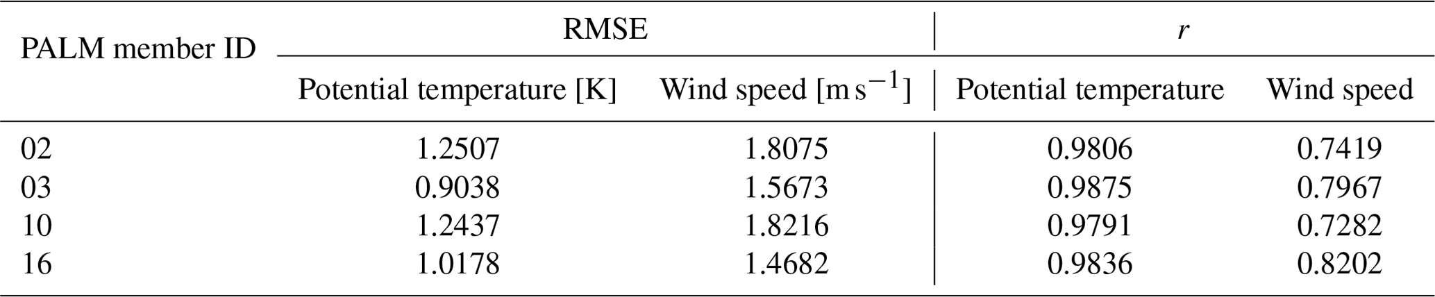
Table D2 April episode PALM ensemble statistical analysis of the potential temperature and wind speed vertical profiles up to the height of 3000 m a.s.l.: root mean square error – RMSE, correlation coefficient – r.

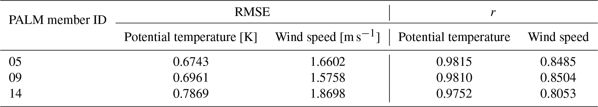
Table D3 July episode PALM ensemble statistical analysis of the potential temperature and wind speed vertical profiles up to the height of 3000 m a.s.l.: root mean square error – RMSE, correlation coefficient – r.

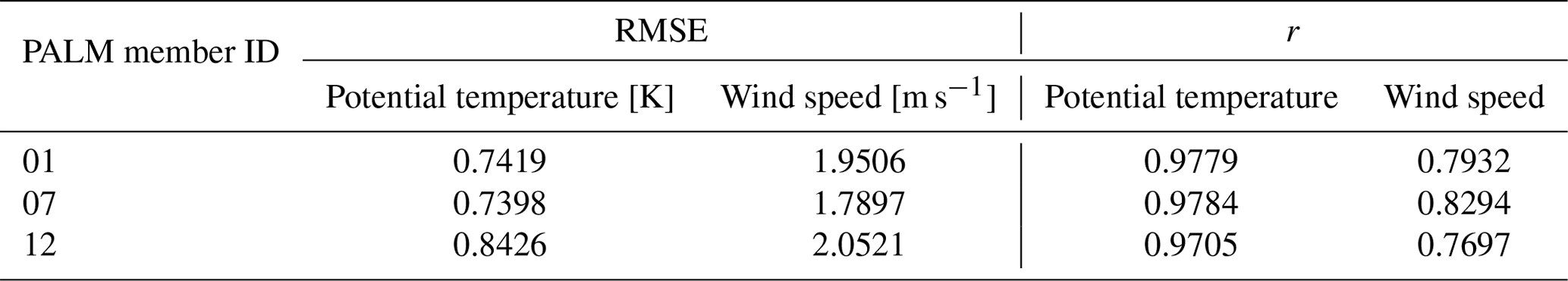
Table D4 October episode PALM ensemble statistical analysis of the potential temperature and wind speed vertical profiles up to the height of 3000 m a.s.l.: root mean square error – RMSE, correlation coefficient – r.

Appendix E: Minimum (min), average (avg), and maximum (max) 72 h averaged differences for air temperature and wind speed for the selected WRF and PALM model outputs

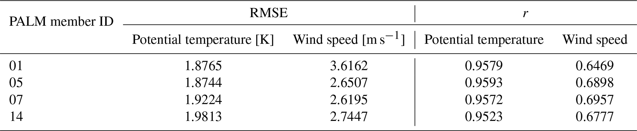
Table E1 February episode minimum (min), average (avg), and maximum (max) 72 h averaged differences for air temperature for the selected WRF and PALM model outputs.

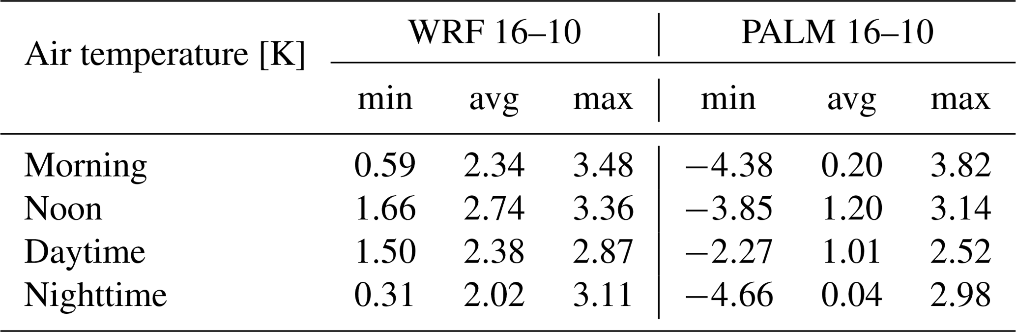
Table E2 February episode minimum (min), average (avg), and maximum (max) 72 h averaged differences for wind speed for the selected WRF and PALM model outputs.

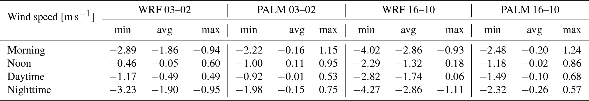
Table E3 April episode minimum (min), average (avg), and maximum (max) 72 h averaged differences for air temperature for the selected WRF and PALM model outputs.

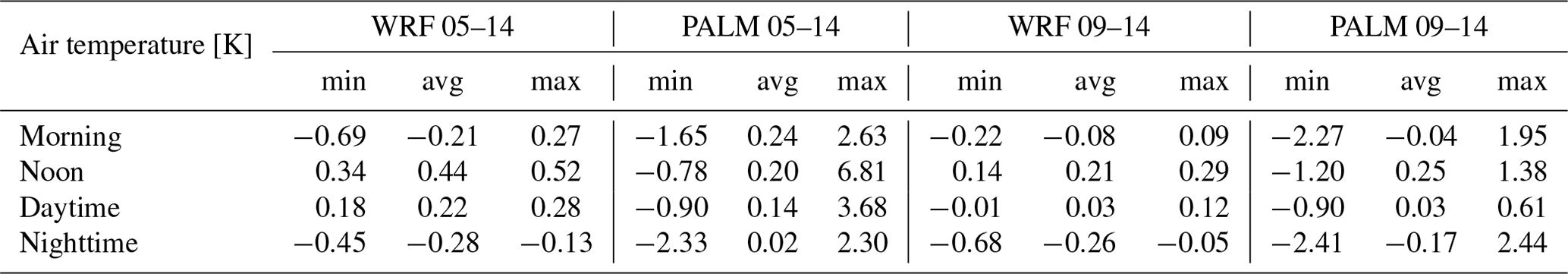
Table E4 April episode minimum (min), average (avg), and maximum (max) 72 h averaged differences for wind speed for the selected WRF and PALM model outputs.

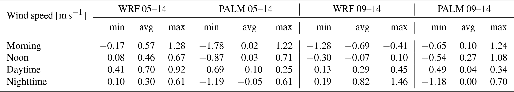
Table E5 July episode minimum (min), average (avg), and maximum (max) 72 h averaged differences for air temperature for the selected WRF and PALM model outputs.

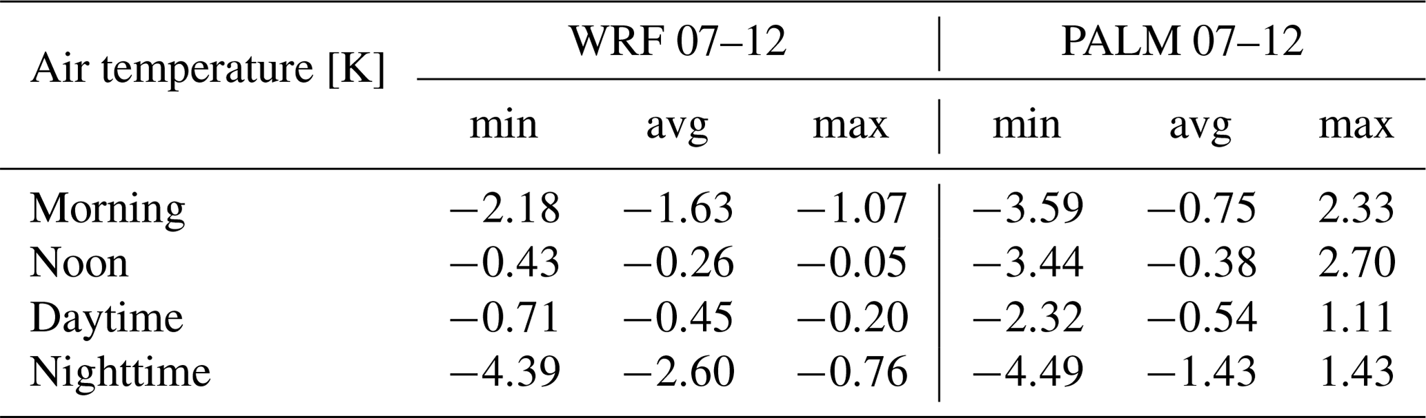
Table E6 July episode minimum (min), average (avg), and maximum (max) 72 h averaged differences for wind speed for the selected WRF and PALM model outputs.

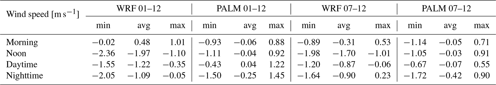
Table E7 July episode minimum (min), average (avg), and maximum (max) 72 h averaged differences for MRT for the selected PALM model outputs.

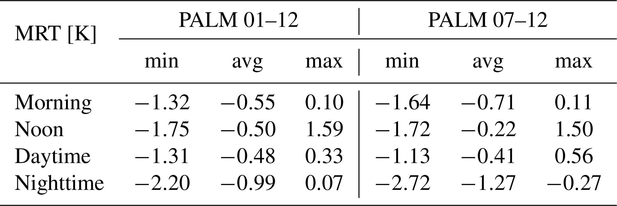
Table E8 July episode minimum (min), average (avg), and maximum (max) 72 h averaged differences for PET for the selected PALM model outputs.

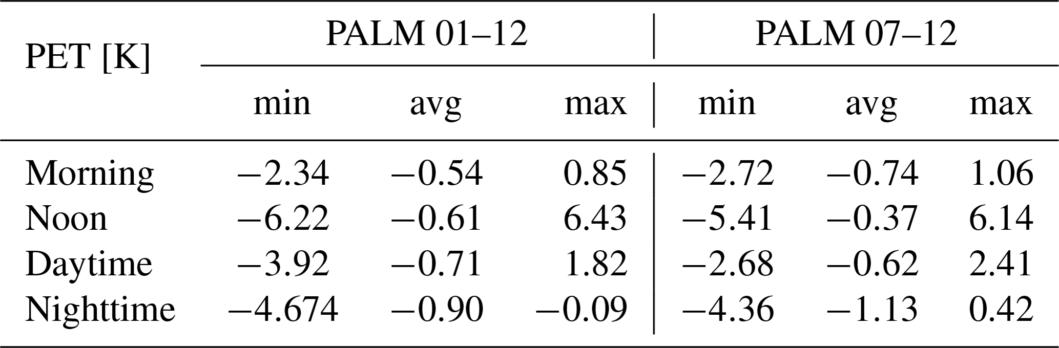
Table E9 October episode minimum (min), average (avg), and maximum (max) 72 h averaged differences for air temperature for the selected WRF and PALM model outputs.

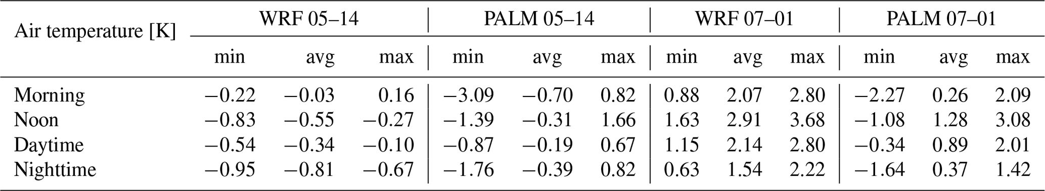
Table E10 October episode minimum (min), average (avg), and maximum (max) 72 h averaged differences for wind speed for the selected WRF and PALM model outputs.

Appendix F: Elevation map of the simulated domain

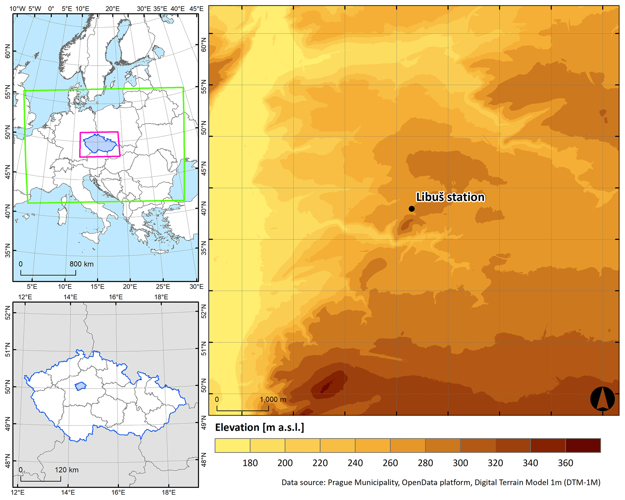
Figure F1 The location of the modeled domain in Europe (top left) and in the Czech Republic (bottom left) and the elevation map of the domain within the city of Prague with the Libuš station (WMO ID 11520) location (right).

Appendix G: Experiment workflow diagram

Figure G1 Experiment workflow diagram.