the Creative Commons Attribution 4.0 License.
the Creative Commons Attribution 4.0 License.
 | 16 Feb 2024
Energy-conserving physics for nonhydrostatic dynamics in mass coordinate models
Mark A. Taylor
Peter A. Bosler
Christopher Eldred
Peter H. Lauritzen
Motivated by reducing errors in the energy budget related to enthalpy fluxes within the Energy Exascale Earth System Model (E3SM), we study several physics–dynamics coupling approaches. Using idealized physics, a moist rising bubble test case, and the E3SM's nonhydrostatic dynamical core, we consider unapproximated and approximated thermodynamics applied at constant pressure or constant volume. With the standard dynamics and physics time-split implementation, we describe how the constant-pressure and constant-volume approaches use different mechanisms to transform physics tendencies into dynamical motion and show that only the constant-volume approach is consistent with the underlying equations. Using time step convergence studies, we show that the two approaches both converge but to slightly different solutions. We reproduce the large inconsistencies between the energy flux internal to the model and the energy flux of precipitation when using approximate thermodynamics, which can only be removed by considering variable latent heats, both when computing the latent heating from phase change and when applying this heating to update the temperature. Finally, we show that in the nonhydrostatic case, for physics applied at constant pressure, the general relation that enthalpy is locally conserved no longer holds. In this case, the conserved quantity is enthalpy plus an additional term proportional to the difference between hydrostatic pressure and full pressure.
- Article
(2460 KB) - Full-text XML
- BibTeX
- EndNote


The primary motivation of this study is to improve energy treatment in the atmospheric component of the Energy Exascale Earth System Model (E3SM) (Golaz et al., 2019, 2022). This component, called the E3SM Atmosphere Model (EAM) (Rasch et al., 2019), is a close cousin of the Community Atmosphere Model (CAM) (Neale et al., 2012) of the Community Earth System Model (CESM), and the design choices regarding thermodynamics in EAM are inherited from CAM (Williamson et al., 2015).
A recently published comprehensive overview by Lauritzen et al. (2022) of thermodynamics in global atmospheric models describes a few deficiencies in EAM/CAM, including the inconsistent treatment of enthalpy (or energy) fluxes of water forms, both within the atmosphere and across its surface boundaries. In particular, there is a large disagreement between the enthalpy fluxes internal to the model as compared to the enthalpy fluxes implied by the associated mass fluxes (Harrop et al., 2022; Lauritzen et al., 2022). This inconsistency is the result of a few design decisions: (1) there is an absence of water forms, except for the water vapor, in the total mass of moist air; (2) specific heat capacities of dry air are used in place of specific heat capacities of water forms; (3) there is a constant moist pressure assumption, which requires a moist pressure adjustment process; (4) each atmospheric process, including the moist pressure adjustment, is required to conserve energy, which has led to the use of fixers; and (5) the atmosphere and surface components explicitly exchange only mass fluxes of water, not energy fluxes.
Some of the abovementioned issues, numbered (1)–(5), are present in other climate models; for example, nearly all of them, except for the Centre National de Recherches Météorologiques Earth system model (CNRM-ESM1) (Séférian et al., 2016; Termonia et al., 2018), use specific heat capacities of dry air for water forms. In the E3SM version 1 (E3SMv1) (Golaz et al., 2019), inconsistency (5) is corrected by a so-called internal energy flux (IEFLX), a global energy flux based on the heat capacity of liquid water. However, by design, IEFLX is another global energy fixer, which balances the energy budget of coupled simulations (i.e., simulations with active atmosphere and ocean components) but does not address all deficiencies in the atmospheric models described above.
To eliminate the need for energy fixers and to properly transfer energy of water forms within the atmosphere and at its interface, we first introduce into the model close to theoretical (or unapproximated) specific heat capacities of water forms and include contributions of all water forms into the moist mass. Second, we reconsider how moist physics packages use the first law of thermodynamics to compute temperature tendencies from phase changes. Interpretations of the first law of thermodynamics in physics–dynamics coupling are the primary focus of this study.
For this, we introduce a few assumptions and considerations and derive coupling mechanisms between the moist physics and the adiabatic dynamical core for constant-pressure and constant-volume approaches. Our constant-pressure approach is an extension of the coupling method that is currently used in EAM/CAM and is applicable to the nonhydrostatic dynamics. For comparison, we also investigate two coupling mechanisms that resemble the coupling in EAM/CAM. One uses the specific heat capacity of the dry air for all species in the moist air, and the other one uses approximated specific heat capacities (in contrast to unapproximated ones mentioned above) of water forms.
Using HOMME, the standalone setup of the dynamical core of EAM, and a simplified moist physics package from Reed and Jablonowski (2012), we provide comparisons of simulations with coupling mechanisms for a test case with a moist rising bubble. This test is commonly used in the literature (Bryan and Fritsch, 2002; Bendall et al., 2020; Liu et al., 2022). Unlike typical large-scale tests for climate modeling, the moist rising bubble test is characterized by an unstable initial state with strong vertical velocities, which quickly trigger phase changes crucial for our studies.
In the setup presented here, we show that the constant-volume and constant-pressure approaches can be significantly different with large time steps. We also show that using approximations where the specific heat function is held constant when computing the latent heat release (as done in EAM's physics parameterizations) always results in large inconsistencies between the change in the atmosphere's energy and the energy flux of sedimentation. Fixing this inconsistency in EAM requires the use of variable latent heats both when computing the latent heat of phase change and when using this heating term to update the temperature.
Many global atmospheric models use a time-split or fractional-step method to separate the dynamics from the physical parameterizations (henceforth referred to as physics), including EAM. In this section, we apply time-splitting to a system of equations, which include phase change and external heating but no external mass fluxes. Splitting the dynamics from the physics, we derive the standard constant-volume and, in the case of hydrostatic dynamics, constant-pressure fractional physics steps with near-exact thermodynamics. In the nonhydrostatic case, the constant-pressure update is inconsistent with the time-split equations, and we derive the nonhydrostatic fractional step based on conservation of energy and on a local heating assumption.
We start by considering a system of equations written as
where X(t) represents a state vector of all our prognostic variables at time t, H represents the dynamical terms, and F represents the forcing terms usually computed by the physics. We use a standard time-split approach and advance the model by one time step Δt via two fractional steps:
with X1 denoting the intermediate state after applying the physics fractional step. System (2)–(3) represents a first order in time approximation to Eq. (1). In this example, both fractional steps are being advanced in time with a forward Euler discretization. In practice, for the dynamics time step, more advanced methods are used, such as HEVI–IMEX (Satoh, 2002; Weller et al., 2013; Lock et al., 2014).
HOMME uses a vertically Lagrangian approach (Lin, 2004). Because of this, each dynamics fractional step (3) can advance from a state X1 given on arbitrary level positions given by geopotential ϕ and mass coordinate values π, based on hydrostatic pressure. This in turn allows us to consider physics fractional steps that arbitrarily change the state variables, including mass, pressure, and volume, within each model layer. Below we consider physics applied either at constant pressure or at constant volume.
To apply time-splitting to our full set of equations, we start with a generic form of the vertically Lagrangian equations with a terrain-following coordinate s and the material derivative .
For completeness, we give the equation of state (EOS) and related mass coordinate identities,
In the above equations, u is the 3D velocity; u3 is the vertical or radial velocity component; T is temperature; p is the full nonhydrostatic pressure; ρ is density with ; ϕ is the geopotential height; π is the mass coordinate/hydrostatic pressure; is the mass coordinate pseudo-density; and qi is a generic total mass mixing ratio that can represent dry air (qd), vapor (qv), liquid water (ql), or ice (qf). For simplicity, we have represented the dynamics terms in the velocity equation by Du. For the HOMME dynamical core used here, the dynamics terms are given in Taylor et al. (2020). We assume the surface elevation, ϕs, is held fixed in time and impose a pressure boundary condition at the model top, taking ptop=πtop, set to a global constant based on the desired vertical domain size. We give two different formulations of the thermodynamic equation, Eqs. (5) and (6). The choice of which one to use depends on whether physics is predominantly applied at constant pressure (δp=0) or at constant volume (δϕ=0).
We use the unapproximated thermodynamics (or variable latent heats, as explained further in Sect. 4.3) from Eldred et al. (2022), which is equivalent to the near-exact thermodynamics from Staniforth (2022). The specific heats and are given in terms of specific heats of dry air, vapor, liquid, and ice and their mixing ratios; R* is a function given in terms of the gas constants for dry air and vapor and their mixing ratios,
and Ll and Lv are latent heat constants. The f* terms in the above represent the forcing tendency terms, where fu corresponds to the momentum fluxes and denotes sources and sinks of water mass from phase changes. The right-hand side of the thermodynamic equation includes the energy flux from phase change (), as well as any external heating denoted by fT. The above equations allow for mass flux between species qi via phase changes but have assumed no net mass flux ().
In this work we focus on the physics fractional step (2) derived from time-splitting Eqs. (4)–(9). We first expand the material derivative into partial derivatives and dynamics terms and then apply time-splitting, with all the f* physics forcing terms put in the physics fractional step (3) and all remaining terms put in the dynamics fractional step (2). We then assume a forward Euler discretization for the physics fractional step partial derivatives, which we represent by δ (as in ). This results in the following physics equations:
where we have again given two formulations of the thermodynamic equation.
2.1 Energy density and column energy
With the unapproximated thermodynamics, the energy density in mass coordinates π can be written as
where we have introduced internal energy () and enthalpy (). The third expression for e given above is useful for certain calculations below and comes from using the identity and the equation of state. The total column energy is given by
where the additional term represents the potential energy of the atmosphere above the model top (ϕtop). We scale all energy integrals by and use a normalized horizontal integral so that the global quantities are in units of J m−2. Conserving the total column energy will take into account the work required to change ϕtop.
Our fractional physics step (12–17) conserves the total column energy E in the sense that the change in E will be given by the net external heating, .
2.2 Constant-volume and constant-pressure updates
From our time-split physics equations (Eqs. 12–17), we see that the only way to obey the geopotential equation (Eq. 15) is to apply physics at constant volume. In Sect. 2.3 we give the constant-volume procedure to update the prognostic variables following Eqs. (12)–(17), which we refer to as the constant-volume update.
We also consider two additional physics updates that are designed for constant pressure, δp=0. In Sect. 2.4 we show that with the hydrostatic equations, which omit Eqs. (7) and (15), time-splitting naturally leads to a δp=0 update. In the nonhydrostatic equations, it is not possible to impose both δp=0 and δϕ=0, and a constant-pressure update cannot be consistent with our physics equations. In Sect. 2.5 we propose an alternative energy-conserving δp=0 update. Despite it being inconsistent with our physics equations, numerical results in Sect. 5 demonstrate that it can be practical. Note that modifying the constant-volume update to obey δp=0 as well is impossible because it leads to an overdetermined system which in general will not have energy-conserving solutions.
For the derivations of these updates, we simplify the algebra by neglecting momentum tendencies by taking fu=0. We also note that for all updates we have δπ=0, which comes from our assumption of no mass fluxes (8).
2.3 The constant-volume update
The constant-volume update is given by the direct application of the time-split system (12–13 and 15–17), with constant volume a direct result of Eq. (15). Combined with our assumption of no mass fluxes, we also have constant density (δα=0). The time-split system reduces to (neglecting the prognostic variables which do not change)
For this update, the model updates qi, , and T to obey the above, and then p is updated from the equation of state, holding ϕ constant. This approach represents a first-order approximation to the original system (Eq. 1); thus it is expected to converge to the correct solution as the time step is decreased. This is the standard physics update used by constant height coordinate models, and it can be straightforwardly used by vertically Lagrangian mass coordinate models. This update conserves energy locally in the sense that the change in energy is given by the external heating (δe=fT), which can be seen directly from Eq. (18).
2.4 The constant-pressure update – hydrostatic
Physics parameterizations are often applied at constant pressure (δp=0). An update which holds pressure constant while allowing the volume to change is impossible to derive via time-splitting for the nonhydrostatic equations, since the prognostic equation for layer positions does not have any traditional physics tendency terms; thus any dynamics/physics time-split approach will lead to δϕ=0 for the update. However, for the hydrostatic equations, which replace Eq. (15) with a diagnostic equation for ϕ (e.g., for CAM/EAM; see Eq. (12.5) in Taylor, 2011), time-splitting the remaining prognostic equations, Eqs. (12), (14), (16), and (17), results in δp=0, and we do have a constant-pressure update, given by
The hydrostatic energy is given by
where eH comes from Eq. (20) and makes use of p=π (total pressure equals to the hydrostatic pressure). The hydrostatic time-split step conserves the hydrostatic column energy in the sense that change in column energy equals the net external heating,
The conservation can be seen by integrating δeH and making use of the fact that the surface elevation ϕsurf remains fixed so that δϕsurf=0.
Changing the volume of a cell does some work on the cells above it, increasing or decreasing their potential energy; thus, any constant-pressure update that conserves column energy will not in general satisfy δe=fT within each cell. For this hydrostatic update, the local changes in energy, internal energy, and enthalpy are given by
2.5 The constant-pressure update – nonhydrostatic
In the nonhydrostatic case, one cannot derive a δp=0 update consistent with the time-split equations since the combination δp=0 and δϕ=0 prohibits changes to any state variables. Instead, we look for a δp=0 update that has the same local energy relation as in the hydrostatic equations,
We start from this form since it automatically conserves the correct column energy as can be seen by expanding δe using Eq. (20) and integrating Eq. (27), as in the hydrostatic case.
Expanding δe using Eq. (20) allows us to write (27) as , which can then be written in terms of our prognostic variables as
where the model updates qi, , and T to obey the above, and then ϕ is updated from the equation of state, holding p constant. For this nonhydrostatic update, the local changes in energy, internal energy, and enthalpy are given by
There are other energy-conserving δp=0 updates, but the update in Eqs. (28)–(29) is unique in that it is the only one where phase change or heating localized to a particular layer will induce temperature changes only in that layer and no other layers (shown in Appendix A). We refer to this condition as local heating. We give an example of a non-local heating update in Appendix B.
Note that for this fractional step, the update of ϕ from the equation of state could be cast as a forcing term for the geopotential equation.
2.6 Dynamical differences between constant pressure and constant volume
A key difference between the constant-pressure and constant-volume approaches is in how latent heat release is translated into physical motion. In the constant-volume approach, during the physics fractional step, each cell's volume and Cartesian position remain fixed, and heating will result in increased pressure. Localized heating will thus result in a pressure gradient, which will induce motion in the dynamics fractional step and in general will result in both vertical and horizontal mass transport. In the constant-pressure approach, in the physics fractional step each cell's pressure will remain constant, and the heating will result in vertical expansion of the cell, representing vertical motion. Localized heating will lead to a gradient in the geopotential, which will induce horizontal motion in the dynamics fractional step.
2.7 Enthalpy formulations of the first law of thermodynamics
The first law of thermodynamics states that the energy of the system is conserved up to fluxes. In the hydrostatic case, the first law under constant-pressure assumption is given by the thermodynamic equation δh=fT. This form of the first law holds across such a wide range of systems that the first law is often interpreted as local conservation of enthalpy. But here, in the nonhydrostatic case for physics processes that are applied at constant pressure, we must change the above thermodynamic equation in order to conserve energy and to obey the first law. In this case, we derive a new thermodynamic equation. When expressed in terms of enthalpy, this energy-conserving thermodynamic equation for nonhydrostatic δp=0 processes can be written as , not δh=fT.
Lauritzen et al. (2022) present an overview of challenges and possible solutions regarding modeling sedimentation. The challenges include interactions of the hydrometeors with the surrounding atmosphere and raise questions about representation of different velocities for different species, falling and not falling, and subsequent frictional heating. In the simple moist physics used here, rain falls out of the atmosphere instantaneously with no additional interactions. As with phase-change physics, we consider sedimentation updates appropriate for constant-pressure and constant-volume approaches. In both cases we hold the temperature constant. In the constant-volume case, we hold volume constant, update π based on the mass flux, and then update the pressure to be consistent with the EOS. We note that the constant-volume sedimentation procedure can be derived from the time-split equations if one generalizes Eqs. (13) or (14) to include additional terms induced by the mass fluxes.
For sedimentation used with constant-pressure physics, we cannot hold the pressure constant due to the mass flux, so we update π based on the mass flux and hold the nonhydrostatic component of the pressure, p−π, constant. We then update the volume to be consistent with the EOS. The constant p−π sedimentation procedure has the advantage that if the state is in hydrostatic balance, it will remain in hydrostatic balance.
This section covers the setup for our numerical simulations with the physics updates introduced in Sect. 2, applied to unapproximated and approximated thermodynamics in a rising bubble test case with a simplified physics package. It also explains that we evaluate energy fluxes due to sedimentation in each simulation by introducing a baseline, a flux of the internal energy of precipitation.
4.1 Description of simple Reed–Jablonowski moist physics
The simple moist physics package from Reed and Jablonowski (2012) consists of a two-stage procedure. First, an amount of condensed water is computed, and a temperature tendency is derived from condensation. For this stage, we compare several different physics updates from Sect. 2. Second, all condensed liquid water is instantaneously removed from the moist air, which can be interpreted as rain falling with infinite speed. For this stage, we use the sedimentation updates given in Sect. 3. In Reed and Jablonowski (2012), for condensation, the temperature tendency given by the conservation of enthalpy is computed using a first-order Taylor series with respect to temperature for the saturation-specific humidity, . Here we instead use vapor tendency explicitly for the current values of T and p.
4.2 Setup of simulations
All runs are performed with the HOMME nonhydrostatic dynamical core with a planar two-dimensional domain (Bogenschutz et al., 2023). The initialization procedure for the moist rising bubble is described in Liu et al. (2022). We use the reference state with θ0=300 K, zero background relative humidity, and domain size of m. In notations used by Liu et al. (2022) the initial conditions for the moist warm bubble are given by the potential temperature perturbation maximum Δθ=4.0 K, the relative humidity perturbation maximum Δh=1.0 (not to be confused with enthalpy h from above), and a cosine-bell perturbation in the form of an ellipse centered at (0,20 00) m, with 5000 m and 1000 m axis lengths for horizontal and vertical directions, respectively. All simulations use 128 vertical levels and 128 fourth-order spectral elements for the horizontal domain (Taylor, 2011), which corresponds to an approximate horizontal resolution of Δx≃52 m.
In simulations, we vary only time step, s, and the physics updates, which are described below in more detail. We consider physics updates with unapproximated thermodynamics, as well as several approximations. In all cases, for energy diagnostics, we use the definition of energy given by Eq. (21).
4.3 Physics updates
Following considerations presented in Sect. 2 that connect conservation of column energy E in Eq. (21) with local temperature updates in parameterizations, we investigate five updates given in Table 1. The first three updates use unapproximated thermodynamics (or variable latent heats), including a constant-volume approach which makes no approximations other than time-splitting. The remaining two updates introduce specific heat-related approximations.
Since latent heats of phase changes are defined as a difference of enthalpies of the two phases (Emanuel, 1994), unapproximated thermodynamics that uses specific heat capacities of water species close to theoretical represents variable (with respect to temperature) latent heats of phase changes. That is, whether we impose variable or constant latent heats depends on the choice of specific heat capacities of water forms.
The first update, named CP-VL-NH, is based on the constant-pressure approach and is formulated as
As explained in Sect. 2, this update conserves Eq. (21). Its alias is translated to constant pressure (CP) and variable latent heats (VL), where variable latent heats means that the correct specific heats for each water species are used in enthalpy expressions. In other words, VL in the name of the update indicates that we use the full unapproximated thermodynamics, including the use of , not (specific heat capacity of the dry air), in Eq. (31). NH in the name of the update stands for nonhydrostatic and denotes that the update conserves nonhydrostatic energy (21). Later, we use HY in the names of updates that conserve only the hydrostatic version of energy (26) and its modifications for updates that use specific heat approximations.
The second update, CV-VL-NH, is the only one presented here that is based on the constant-volume (CV) approach. It is given by
where, similarly to CP-VL-NH, we use variable latent heats. As explained in Sect. 2, this update conserves Eq. (21).
The third update, CP-VL-HY, is a slight modification of CP-VL-NH,
It is of interest because we suspect that the nonhydrostatic term in Eq. (31) is negligible. The results from both CP-VL-NH and CP-VL-HY prove to be indistinguishable for our rising bubble test case.
The other two updates, CP-CL-HY and CP-AL-HY, are inspired by the EAM design. CP-CL-HY is given by
and mimics the current EAM. Its name is based on constant latent heats (CL), since the update uses , not .
Since it would require a significant effort to rewrite moist parameterizations in EAM for update (31), one could consider a design where temperature tendencies from a parameterization are computed using instead of , but is held constant during the phase-change physics and only updated after sedimentation. Thus, the CP-AL-HY update is given by
The shorthand AL in its name indicates that only approximate variable latent heats are used.
As for the other updates above, for updates CP-CL-HY and CP-AL-HY we use the definition of the total column energy (21) when computing energy diagnostics.
Table 1List of physics updates considered. CP and CV stand for constant pressure and constant volume, VL denotes variable latent heats, CL denotes constant latent heats, and AL is for approximate latent heats. HY stands for hydrostatic and NH stands for nonhydrostatic. For more details on updates, see Sect. 4.3. The choice of Tref is explained in Sect. 4.4. P denotes precipitation mass flux. The energy flux discrepancy is the difference between the change in the total atmosphere energy () and the energy carried out of the model from precipitation (FP), as explained in Sects. 4.4 and 5.
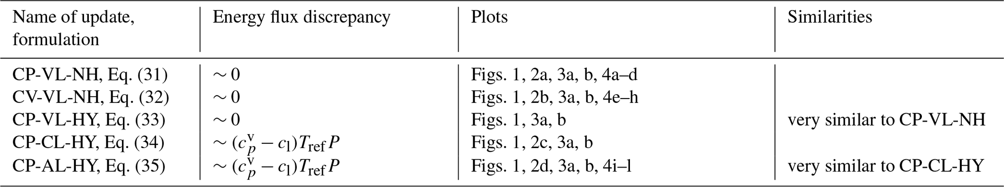
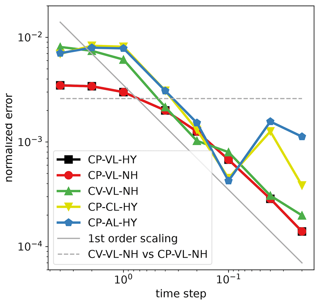
Figure 1Self-convergence with respect to time step for all five updates using definition (37). Uncertainty, presented by the horizontal dashed line, is the normalized difference between the reference solutions for simulations with CP-VL-NH (red curve) and CV-VL-NH (green curve). Other curves are CP-VL-HY (black), CP-AL-HY (blue), and CP-CL-HY (yellow).
4.4 Energy of precipitation and its relation to change of energy in the model
As mentioned in the Introduction, in EAM there is a large disagreement between the change in atmospheric energy as compared to the net flux of energy carried into and out of the model by evaporation and precipitation. This error is significant, and in order to balance the energy budget for simulations with an active ocean component a global fixer must be used (Golaz et al., 2019).
To examine this error in our idealized setup, we look at the total atmospheric energy changes for each of the updates in Table 1 and compare them to the approximate flux FP coming from the internal energy of the precipitation P,
Per discussions in Lauritzen et al. (2022), we define Eq. (36) not with varying temperature but with constant temperature, Tref. Obviously, the true energy flux from precipitation would not be described by Eq. (36). However, Eq. (36) is a very good approximation for the energy of precipitation, as shown in Golaz et al. (2019) and later by our simulations. Using it gives us the same baseline to compare energy of precipitation for simulations with different updates.
Note that definition (36) does not include terms with Lv or Ll from Eq. (18). The energy of precipitation corresponding to these terms in all updates in Table 1 (as well as in EAM) is treated accurately, unlike the terms that correspond to internal or potential energy. Therefore, in our analysis we focus only on the discrepancy between the globally integrated energy flux without L terms , where and FP is defined by Eq. (36).
Based on the results from our simulations presented below, we conclude that only updates with full variable latent heats, which correctly treat internal energy of liquid water, accurately represent energy of precipitation.
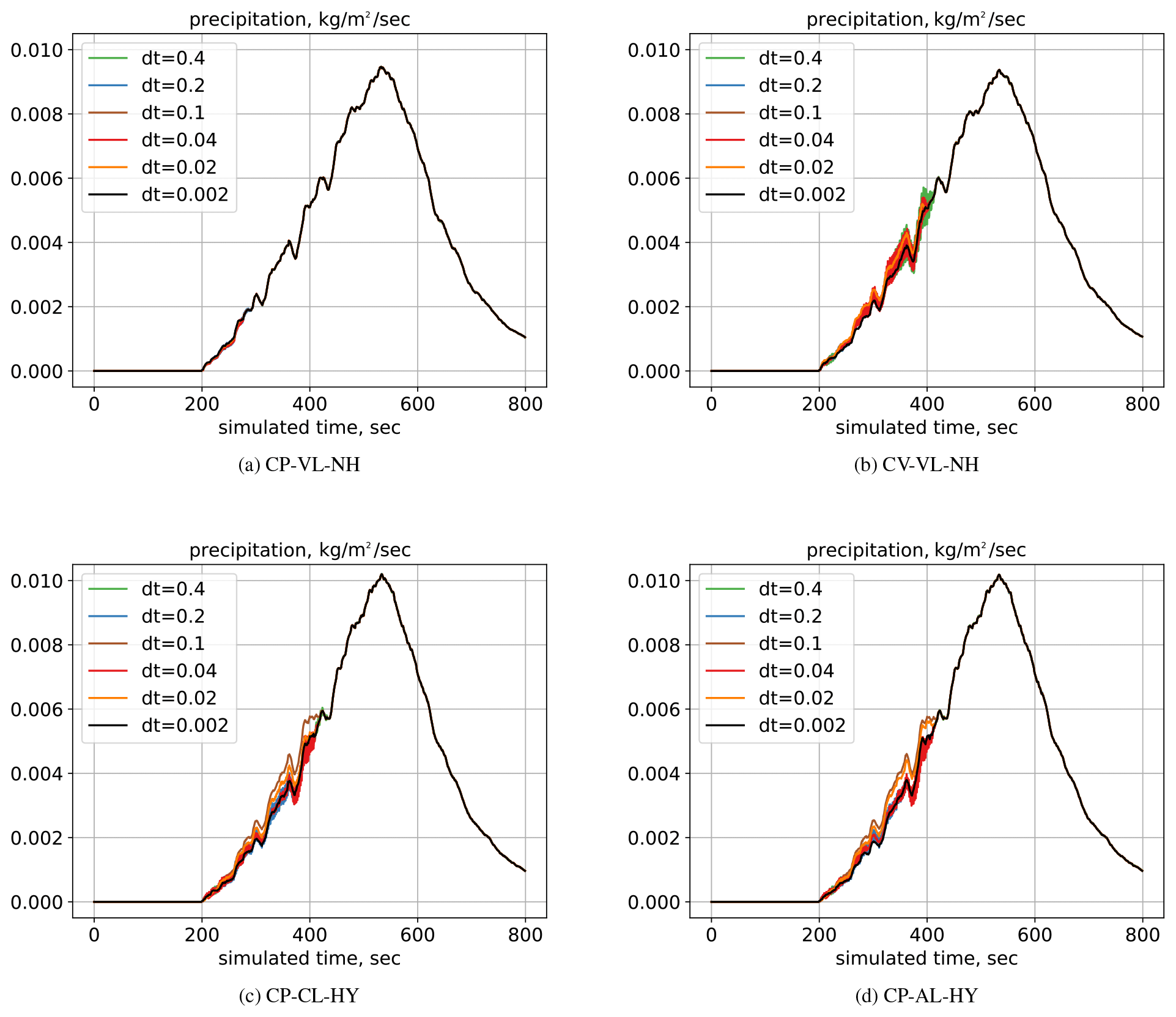
Figure 2Globally integrated over the domain precipitation rate for different updates for different Δt (given in the labels in seconds) with respect to simulated time (horizontal axes). A plot for CP-VL-HY is not shown, but it is identical to plot (a) for CP-VL-NH.
5.1 Time step convergence
We first examine the error introduced by the physics–dynamics time-splitting. To do this, we consider a fixed spatial discretization so that our system of equations can be represented as a system of ordinary differential equations (ODEs), and we consider the discretization of these ODEs in time. We study the convergence of this ODE system as the time step goes to zero. This approach follows Wan et al. (2015), where CAM physics is shown to converge with respect to time step with fixed horizontal resolution. The time discretization includes the time-splitting error and the truncation error in the forward Euler method used for the physics step and in the Runge–Kutta method used for the dynamics step. These errors are all formally first order or better in Δt; thus, if the ODE has a solution, we expect our discretization to converge to this solution with first-order accuracy.
For each update in Table 1, we perform simulations with time step Δt varying from 4.0 to 0.002 s, as given in Sect. 4.2. Simulations with 0.002 s are used as reference solutions for convergence studies. Per discussion in Sect. 2, we do not expect the two unapproximated updates (CP-VL-NH and CV-VL-NH) to converge to the same unique solution, since only CV-VL-NH is consistent with the time-split approach. Nor do we expect the different approximated updates (CP-VL-HY, CP-CL-HY, and CP-AL-HY) to agree with any of the other updates. Instead, we study self-convergence for each update, defining the error with respect to each update's own reference solutions via
where a set of θi represents a potential temperature field from a simulation with Δt>0.002 s, θref,i is the potential temperature field given by a reference solution with Δt=0.002 s, and ai represents the horizontal area weights associated with each nodal value. Sets θi and θref,i are remapped to a uniform-in-height vertical grid for the domain [0,15 000] m, and a few horizontal levels at the top and at the bottom of the domain are discarded. The error is computed at t=800 s after the bubble has evolved quite substantially. Plots of θ at t=800 s are shown below in Fig. 4.
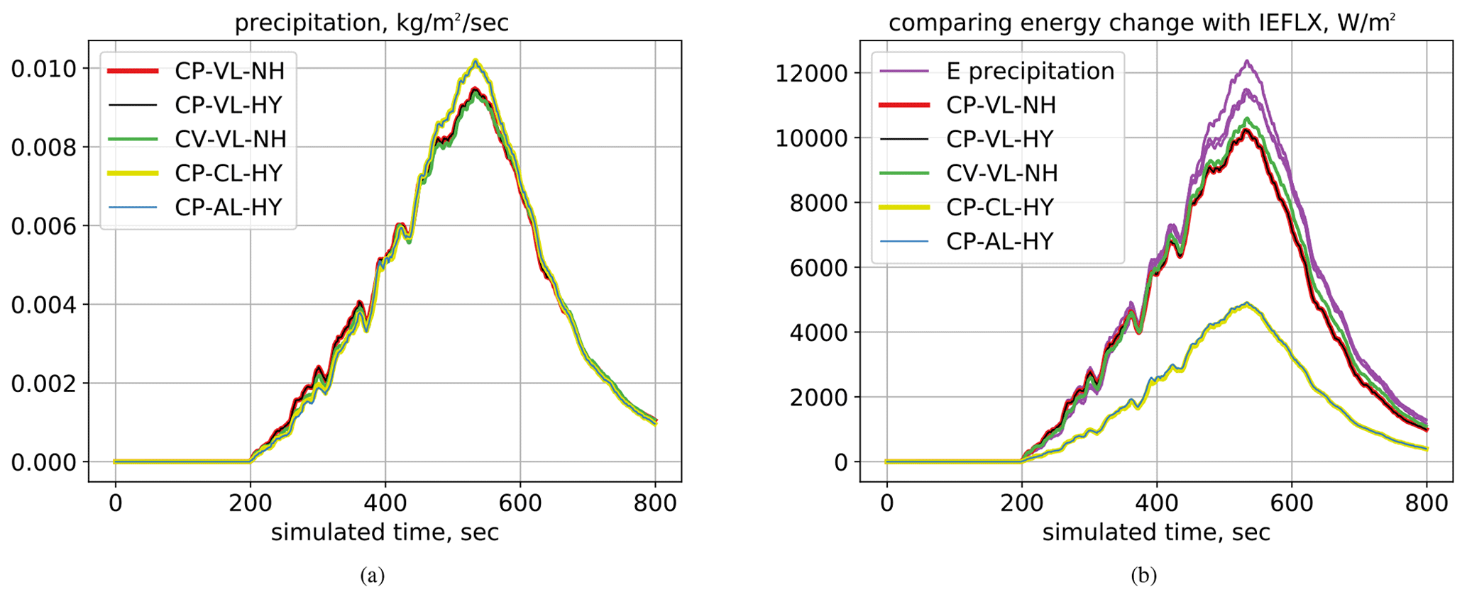
Figure 3Plot (a) contains globally integrated mass fluxes for all simulations for Δt=0.002 s, and these fluxes are very similar for all simulations. Plot (b) compares the outflux of energy of precipitation, FP (in purple, given by Eq. (36)), and Et, both globally integrated, for simulations with Δt=0.002 s for all five updates.
In Fig. 1 we present self-convergence results for all five updates. There CP-VL-NH and CP-VL-HY are given by red and black curves, which are practically identical. CV-VL-NH is represented by the green curve. All of the VL updates show the expected first-order convergence and have similar errors for small time steps, although CV-VL-NH has noticeably larger errors for large time steps, which does result in visible differences in θ that are shown below in Fig. 4. The convergence of the non-VL updates, CP-AL-HY and CP-CL-HY, is given by blue and yellow curves. These updates have similar errors and show the expected first-order convergence down to about four digits but then fail to continue to converge.
We consider the reference solution for the CV-VL-NH update the most accurate. For our fixed spatial discretization, the only remaining discretization errors in the CV-VL-NH update come from time discretization and are driven to zero by time step convergence as shown in Fig. 1. The CP-VL-NH update has an additional source of error in that it applies a constant-pressure assumption, which is not consistent with the time-split equations. To approximate this error, we measure the difference between the CP-VL-NH and CV-VL-NH reference solutions using Eq. (37). At t=800 s, this difference is 0.0026 (shown as the dashed line in Fig. 1). For these two VL updates, the potential temperature fields agree to more than three digits and are visually very close, as shown below in Fig. 4. We consider this difference a crude estimate of the uncertainty introduced by imposing the constant-pressure constraint in the physics update.
Figure 2 shows the time evolution of the globally integrated over the domain precipitation rates P for CP-VL-NH (panel a), CV-VL-NH (panel b), CP-CL-HY (panel c), and CP-AL-HY (panel d) plotted against the simulated time for each time step. A plot for CP-VL-HY is nearly identical to the plot for CP-VL-NH, and the two reference solutions for these two updates differ by only using Eq. (37), so, CP-VL-HY is not included in the figure. Precipitation plots can be used to evaluate the sensitivity of each update with respect to different time steps. Qualitatively, all updates have very similar global precipitation rates. We note that the two constant-pressure VL updates (panel a) have very little sensitivity, significantly lower than the remaining updates (panels b–d), which we consider to be an advantage of CP-VL-NH or CP-VL-HY.
5.2 Energy flux discrepancy
Next we compare energy flux and the approximate precipitation energy flux FP as given by Eq. (36), both globally integrated over the domain, for the reference solutions for each of five updates. Since FP depends on the mass of precipitation, we first confirm that overall globally integrated over the domain mass fluxes from precipitation for all simulations are reasonably close to each other, as shown in Fig. 3a. There, CP-VL-NH (red), CP-VL-HY (black), and CV-VL-NH (green) curves are clustered together, while the non-VL methods, CP-AL-HY (blue) and CP-CL-HY (yellow), are positioned separately from the other three but next to each other. In Fig. 3b, we first plot in purple FP computed for the precipitation rates of each simulation. Then we plot , where is the difference of the total energy of the model (given by Eq. (21) and summed for all columns) for before and after the physics fractional step, adjusted for L terms as discussed in Sect. 4.4. As expected, energy fluxes from the unapproximated VL updates, CP-VL-NH (red), CP-VL-HY (black), and CV-VL-NH (green), are very close to FP. A small difference between FP and for these three updates is due to the temperature variations; the temperature of precipitation in the simulations is slightly smaller than Tref. Another term that possibly could affect the difference between FP and is the potential temperature of precipitation, but it is negligible compared to its internal energy.
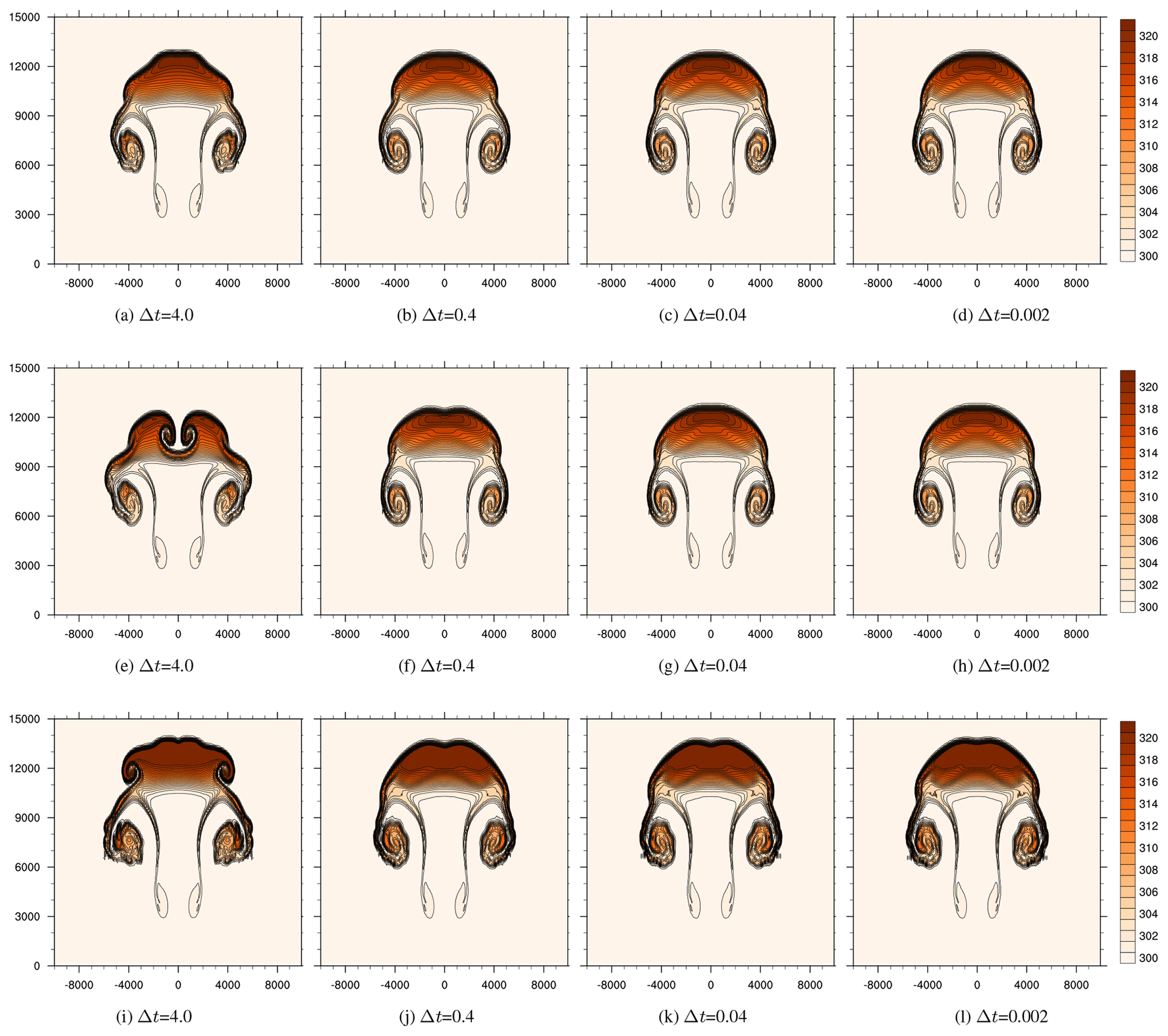
Figure 4Potential temperature field in Kelvin for CP-VL-NH (a–d), CV-VL-NH (e–h), and CP-AL-HY (i–l). The units for time steps Δt in the captions are seconds.
For the non-VL updates CP-AL-HY (blue) and CP-CL-HY (yellow), which have nearly identical values of , the difference between and FP is significant,
Since and cl=4188.0 J kg−1 K−1, we see that error is 50 % of the desired flux clPTref. This is due to the fact that the originally precipitating water in the model is represented by water vapor, with its enthalpy approximately given by . For both the AL and the CL updates, the phase change physics followed by sedimentation appears to remove vapor from the atmosphere instead of liquid water, which results in , which in turn leads to (38). In other words, the discrepancy between energies of precipitable water and in CP-AL-HY and CP-CL-HY is due to the fact that the energy of the liquid water is not properly accounted for throughout the physics update.
5.3 Qualitative comparisons
Figure 4 plots the potential temperature of the bubble at the end of the simulated time, 800 s, for three updates, CP-VL-NH (top row), CV-VL-NH (middle row), and CP-AL-HY (bottom row). The results in each column correspond to a different time step size, Δt=4.0, 0.4, 0.04, and 0.002 s, from left to right. Note that simulations with a 0.002 s time step (the rightmost column) are the reference solutions from the convergence plot in Fig. 1. Bubbles from CP-VL-HY and CP-CL-HY are not shown: CP-VL-HY plots are identical to the bubbles from CP-VL-NH, and CP-CL-HY bubbles are very similar to the bubbles from CP-AL-HY.
One of the most interesting observations is that while bubbles for CP-VL-NH and CV-VL-NH at smaller time steps are very similar, their trajectories towards the reference solutions differ. The shapes in the constant-pressure approach become indistinguishable starting at a time step of 0.4 s, while for the constant-volume approach, only the solution for the 0.04 s time step is comparable to the reference solution by eye. In other words, if we consider either reference solution, in panel (d) or panel (h), acceptable, then for this particular test case CP-VL-NH appears more accurate than CV-VL-NH when using large time steps.
Separately, for the coarse 4.0 s time steps, the bubble in the constant-volume simulation is more distorted and more turbulent than the bubble from CP-VL-NH. It is explained in Sect. 2 that in CV-VL-NH, the energy from condensation is not transferred into moving vertical layers until the dynamics fractional step, while in the case of the constant-pressure approach, a part of this energy transfers into vertical motion during the physics fractional step.
Compared to the first two rows, the bubbles from CP-AL-HY in panels (i)–(l) (and CP-CL-HY, not shown) appear to be warmer and, as a result, moving upward faster, consistent with their approximated temperature update.
The primary focus of this paper is to study different updates in Table 1 at the condensation stage in physics. One could argue that in this case, all simulations should use the same sedimentation routine. To investigate this further, we performed simulations with CV-VL-NH for condensation and the constant-pressure sedimentation. The quantitative results of such simulations and plots are almost identical to those presented. For example, there are no detectable differences in the green convergence curve in Fig. 1. There are only very minor differences for the precipitation and energy flux plots in Figs. 2 and 3. For the bubble plots in the middle row of Fig. 4, switching to the constant-pressure sedimentation does not affect the overall structures of the bubbles. It also does not change our conclusions about computational feasibility of the simulations with CV-VL-NH. Therefore, for simulations with condensation based on CV-VL-NH, we chose to apply a sedimentation routine based on the constant-volume approach, too, since both obey a time-split integration concept.
Moist physics packages are designed to conserve energy from phase changes of water forms. A particular form of conservation rule defines how state variables like temperature, pressure, and geopotential are updated during physics–dynamics coupling. We focus on the two most common approaches, constant pressure and constant volume. Considering that the current EAM design is based on a time-split integration of physics and dynamics, our analysis shows that for the nonhydrostatic model, the constant-volume approach is consistent with the underlying system of equations, while the constant-pressure approach is not. The constant-pressure approach is attractive for global models since if the initial state is in hydrostatic balance, this balance will be preserved by the physics update, including in the presence of mass fluxes such as sedimentation.
Thermodynamic processes which occur at constant pressure are often shown to locally conserve enthalpy, meaning that changes in enthalpy match the external forcing, and the thermodynamic equation can be written as δh=fT. This relation holds very generally, including in the hydrostatic equations, but it will not conserve energy in the nonhydrostatic equations. For the nonhydrostatic equations we derive the constant-pressure energy-conserving update and show that this is the unique update which has the additional property that external heating and phase change will only result in local temperature changes. In the rising bubble test case used here, the effect of this correction was negligible.
In order to have the model's energy budget properly account for the energy of the precipitation flux, we study effects of variable, constant, and approximate latent heats during phase transitions in physics. We show that only by using variable latent heats throughout the physics computations can one expect correct accounting of energy fluxes from precipitation. To extend our conclusions for more practical applications like EAM, proper modeling of water energy fluxes would require updating both the moist physics packages and the code which applies the physics tendencies to incorporate unapproximated thermodynamics of water forms.
In this section we give the derivation of the unique nonhydrostatic δp=0 update, Eqs. (28)–(29), which will conserve column energy and ensure a concept of local heating. We consider the model presented in Sect. 2 with both phase changes and external heating fT but no net mass flux or momentum flux. The phase changes are given by with associated heating . We then seek updates for T and ϕ that obey the following constraints:
-
constant pressure (δp=0);
-
conservation of column energy ();
-
local heating, meaning that latent heat and other sources of external heating will be applied locally, in particular, in regions with and fT(π)=0, then δT(π)=0.
In Sect. 2.5, we show that under the δp=0 constraint, the update given by conserves column energy. By inspection one can also see that it obeys the local heating constraint. To show that such an update is unique, we now show the converse: if one assumes δp=0, conservation of the column energy, and local heating, then it must be that .
Given the first two requirements, and using Eq. (20), we start with conservation of column energy,
Since we are not considering momentum flux or external mass flux, we have . Combined with δp=0, we derive
where we have introduced Q to denote the sum of the latent and external forcing terms. This integral relation must hold for all possible Q. Combined with our third requirement (δT=0 where and fT=0) we can show that this integral relation can only hold for all Q if the integrands in Eq. (A2) are equal. To see this in the discrete case, consider heating only in a single arbitrary model layer [π1,π2]. Outside that model layer we have no phase change (), and also fT=0; thus δT=0 by our local heating assumption. Thus, outside this region, both integrands are zero, and the integral relation for energy conservation reduces to an integral over the single model layer [π1,π2],
The discrete version of this integral is computed as dπ times the layer midpoint values of the integrand; thus these layer midpoint values must be equal, and we have that must hold at every model layer. This equation is equivalent to Eqs. (28)–(29) and the different forms given in Eq. (30). In the continuum, a similar argument can be made by choosing a sequence of Q's which converge to a Dirac delta function at an arbitrary layer π and by examining the convergence of Eq. (A2) with respect to this sequence.
Here we investigate other ways to derive constant-pressure updates for the nonhydrostatic model and how the form of the update is connected to the form of the first law of thermodynamics.
In Sect. 2.5 we derive update CP-VL-NH by considering the energy equation
which leads to the internal energy equation . In the literature, the first law of thermodynamics is often presented as with quantity pδα defined as the pressure work, but this version of the thermodynamic equation does not conserve column energy (21) for constant-pressure processes. It follows that in update CP-VL-NH the pressure work is given by quantity , not pδα.
One can be motivated to explore a constant-pressure update with the right-hand side given by in Eq. (B1). Following Sect. 2, the formulations of this update in terms of e, ei, and h are given by
Therefore, this update has yet another definition of the pressure work, . We attribute inconsistencies in the definition of the pressure work in NH constant-pressure updates as compared to quantity pδα to the fact that these updates do not obey a time-split approach and thus violate our thermodynamic equation (Eq. 13).
As noted in Sect. 2, update (B2) cannot be local. Consider that, in the whole vertical column of the model, there is only one vertical level where a phase change triggers heat release. Then the level expands and the geopotential for the levels above it changes, too. To conserve the total column energy, the h equation from (B2) needs to be satisfied at those levels, which leads to a temperature tendency at levels without a phase change. However, if the locality of the update is not essential for the computational performance, it is to be defined whether update CP-VL-NH is preferable to the update (B2) or to any other non-local update.
The code was developed as a part of the dynamical core (HOMME) code base, which itself is a part of the E3SM repository and is available under a BSD 3-clause license. The code, running scripts, and plotting scripts are archived at https://doi.org/10.5281/zenodo.8336379 (Foucar et al., 2023). For instructions, navigate to file components/homme/docs-to-save-for-paper-provinance-july22/HOW-TO-MAKE-PAPER-PLOTS. Plotting and running scripts use NCL and Python.
All authors contributed to conceptualization and article writing. OG and MAT derived the algorithms. OG implemented the algorithms in HOMME and ran the numerical studies.
The contact author has declared that none of the authors has any competing interests.
Publisher's note: Copernicus Publications remains neutral with regard to jurisdictional claims made in the text, published maps, institutional affiliations, or any other geographical representation in this paper. While Copernicus Publications makes every effort to include appropriate place names, the final responsibility lies with the authors.
We thank the article reviewers for their helpful and constructive comments.
Sandia National Laboratories is a multi-mission laboratory managed and operated by National Technology & Engineering Solutions of Sandia, LLC (NTESS), a wholly owned subsidiary of Honeywell International Inc., for the U.S. Department of Energy's National Nuclear Security Administration (DOE/NNSA) under contract DE-NA0003525. This written work is authored by an employee of NTESS. The employee, not NTESS, owns the right, title, and interest in and to the written work and is responsible for its contents. Any subjective views or opinions that might be expressed in the written work do not necessarily represent the views of the U.S. Government. The publisher acknowledges that the U.S. Government retains a non-exclusive, paid-up, irrevocable, world-wide license to publish or reproduce the published form of this written work or allow others to do so, for U.S. Government purposes. The DOE will provide public access to results of federally sponsored research in accordance with the DOE Public Access Plan.
This research used a high-performance computing cluster provided by the DOE Office of Science, Office of Biological and Environmental Research Earth Systems Model Development Program area of Earth and Environmental System Modeling and operated by the Laboratory Computing Resource Center at Argonne National Laboratory.
This work was supported by the US Department of Energy (DOE) Office of Science's Advanced Scientific Computing Research (ASCR) and Biological and Environmental Research (BER) Programs under the Scientific Discovery through Advanced Computing (SciDAC 4) ASCR/BER Partnership Program. This research was also supported as part of the Energy Exascale Earth System Model (E3SM) project, funded by BER Earth Systems Model Development Program area of Earth and Environmental System Modeling.
This paper was edited by Yongze Song and reviewed by Thomas Bendall and three anonymous referees.
Bendall, T. M., Gibson, T. H., Shipton, J., Cotter, C. J., and Shipway, B.: A compatible finite-element discretisation for the moist compressible Euler equations, Q. J. Roy. Meteor. Soc., 146, 3187–3205, https://doi.org/10.1002/qj.3841, 2020. a
Bogenschutz, P. A., Eldred, C., and Caldwell, P. M.: Horizontal Resolution Sensitivity of the Simple Convection-Permitting E3SM Atmosphere Model in a Doubly-Periodic Configuration, J. Adv. Model. Earth Sy., 15, e2022MS003466, https://doi.org/10.1029/2022MS003466, 2023. a
Bryan, G. H. and Fritsch, J. M.: A Benchmark Simulation for Moist Nonhydrostatic Numerical Models, Mon. Weather Rev., 130, 2917–2928, https://doi.org/10.1175/1520-0493(2002)130<2917:ABSFMN>2.0.CO;2, 2002. a
Eldred, C., Taylor, M., and Guba, O.: Thermodynamically consistent versions of approximations used in modelling moist air, Q. J. Roy. Meteor. Soc., 148, 3184–3210, https://doi.org/10.1002/qj.4353, 2022. a
Emanuel, K.: Atmospheric Convection, Oxford University Press, ISBN 9780195066302, https://doi.org/10.1002/qj.49712152516, 1994. a
Foucar, J., Edwards, J., Petersen, M., Bertagna, L., Hoffman, M., Jacobsen, D., Wolfe, J., Mametjanov, A., Duda, M., Jacob, R., singhbalwinder, AaronDonahue, Taylor, M., Hillman, B. R., Sacks, B., onguba, for E3SM related projects, A., Asay-Davis, X., Hannah, W., Turner, A. K., noel, Bradley, A. M., jayeshkrishna, Roekel, L. V., fischer ncar, Paul, K., Ringler, T., Deakin, M., Turner, M., and ldfowler58: oksanaguba/E3SM: support-materials5, Zenodo [code], https://doi.org/10.5281/zenodo.8336379, 2023. a
Golaz, J.-C., Caldwell, P. M., Roekel, L. P. V., Petersen, M. R., Tang, Q., Wolfe, J. D., Abeshu, G., Anantharaj, V., Asay-Davis, X. S., Bader, D. C., Baldwin, S. A., Bisht, G., Bogenschutz, P. A., Branstetter, M., Brunke, M. A., Brus, S. R., Burrows, S. M., Cameron-Smith, P. J., Donahue, A. S., Deakin, M., Easter, R. C., Evans, K. J., Feng, Y., Flanner, M., Foucar, J. G., Fyke, J. G., Griffin, B. M., Hannay, C., Harrop, B. E., Hunke, E. C., Jacob, R. L., Jacobsen, D. W., Jeffery, N., Jones, P. W., Keen, N. D., Klein, S. A., Larson, V. E., Leung, L. R., Li, H.-Y., Lin, W., Lipscomb, W. H., Ma, P.-L., Mahajan, S., Maltrud, M. E., Mametjanov, A., McClean, J. L., McCoy, R. B., Neale, R. B., Price, S. F., Qian, Y., Rasch, P. J., Eyre, J. J. R., Riley, W. J., Ringler, T. D., Roberts, A. F., Roesler, E. L., Salinger, A. G., Shaheen, Z., Shi, X., Singh, B., Tang, J., Taylor, M. A., Thornton, P. E., Turner, A. K., Veneziani, M., Wan, H., Wang, H., Wang, S., Williams, D. N., Wolfram, P. J., Worley, P. H., Xie, S., Yang, Y., Yoon, J.-H., Zelinka, M. D., Zender, C. S., Zeng, X., Zhang, C., Zhang, K., Zhang, Y., Zheng, X., Zhou, T., and Zhu, Q.: The DOE E3SM coupled model version 1: Overview and evaluation at standard resolution, J. Adv. Model. Earth Sy., 11, 2089–2129, https://doi.org/10.1029/2018ms001603, 2019. a, b, c, d
Golaz, J.-C., Van Roekel, L. P., Zheng, X., Roberts, A. F., Wolfe, J. D., Lin, W., Bradley, A. M., Tang, Q., Maltrud, M. E., Forsyth, R. M., Zhang, C., Zhou, T., Zhang, K., Zender, C. S., Wu, M., Wang, H., Turner, A. K., Singh, B., Richter, J. H., Qin, Y., Petersen, M. R., Mametjanov, A., Ma, P.-L., Larson, V. E., Krishna, J., Keen, N. D., Jeffery, N., Hunke, E. C., Hannah, W. M., Guba, O., Griffin, B. M., Feng, Y., Engwirda, D., Di Vittorio, A. V., Dang, C., Conlon, L. M., Chen, C.-C.-J., Brunke, M. A., Bisht, G., Benedict, J. J., Asay-Davis, X. S., Zhang, Y., Zhang, M., Zeng, X., Xie, S., Wolfram, P. J., Vo, T., Veneziani, M., Tesfa, T. K., Sreepathi, S., Salinger, A. G., Reeves Eyre, J. E. J., Prather, M. J., Mahajan, S., Li, Q., Jones, P. W., Jacob, R. L., Huebler, G. W., Huang, X., Hillman, B. R., Harrop, B. E., Foucar, J. G., Fang, Y., Comeau, D. S., Caldwell, P. M., Bartoletti, T., Balaguru, K., Taylor, M. A., McCoy, R. B., Leung, L. R., and Bader, D. C.: The DOE E3SM Model Version 2: Overview of the Physical Model and Initial Model Evaluation, J. Adv. Model. Earth Sy., 14, e2022MS003156, https://doi.org/10.1029/2022MS003156, 2022. a
Harrop, B. E., Pritchard, M. S., Parishani, H., Gettelman, A., Hagos, S., Lauritzen, P. H., Leung, L. R., Lu, J., Pressel, K. G., and Sakaguchi, K.: Conservation of Dry Air, Water, and Energy in CAM and Its Potential Impact on Tropical Rainfall, J. Climate, 35, 2895–2917, https://doi.org/10.1175/JCLI-D-21-0512.1, 2022. a
Lauritzen, P. H., Kevlahan, N. K.-R., Toniazzo, T., Eldred, C., Dubos, T., Gassmann, A., Larson, V. E., Jablonowski, C., Guba, O., Shipway, B., Harrop, B. E., Lemarié, F., Tailleux, R., Herrington, A. R., Large, W., Rasch, P. J., Donahue, A. S., Wan, H., Conley, A., and Bacmeister, J. T.: Reconciling and Improving Formulations for Thermodynamics and Conservation Principles in Earth System Models (ESMs), J. Adv. Model. Earth Sy., 14, e2022MS003117, https://doi.org/10.1029/2022MS003117, 2022. a, b, c, d
Lin, S.-J.: A Vertically Lagrangian Finite-Volume Dynamical Core for Global Models, Mon. Weather Rev., 132, 2293–2397, 2004. a
Liu, W., Ullrich, P. A., Guba, O., Caldwell, P. M., and Keen, N. D.: An Assessment of Nonhydrostatic and Hydrostatic Dynamical Cores at Seasonal Time Scales in the Energy Exascale Earth System Model (E3SM), J. Adv. Model. Earth Sy., 14, e2021MS002805, https://doi.org/10.1029/2021MS002805, 2022. a, b, c
Lock, S.-J., Wood, N., and Weller, H.: Numerical analyses of Runge-Kutta implicit-explicit schemes for horizontally explicit, vertically implicit solutions of atmospheric models, Q. J. Roy. Meteor. Soc., 140, 1654–1669, https://doi.org/10.1002/qj.2246, 2014. a
Neale, R. B., Chen, C.-C., Gettelman, A., Lauritzen, P. H., Park, S., Williamson, D. L., Conley, A. J., Garcia, R., Kinnison, D., Lamarque, J.-F., Marsh, D., Mills, M., Smith, A. K., Tilmes, S., Vitt, F., Morrison, H., Cameron-Smith, P., Collins, W. D., Iacono, M. J., Easter, R. C., Ghan, S. J., Liu, X., Rasch, P. J., and Taylor, M. A.: Description of the NCAR Community Atmosphere Model (CAM 5.0), https://www.cesm.ucar.edu/models/cesm1.0/cam/docs/description/cam5_desc.pdf (last access: 2 July 2021), 2012. a
Rasch, P. J., Xie, S., Ma, P.-L., Lin, W., Wang, H., Tang, Q., Burrows, S. M., Caldwell, P., Zhang, K., Easter, R. C., Cameron-Smith, P., Singh, B., Wan, H., Golaz, J.-C., Harrop, B. E., Roesler, E., Bacmeister, J., Larson, V. E., Evans, K. J., Qian, Y., Taylor, M., Leung, L. R., Zhang, Y., Brent, L., Branstetter, M., Hannay, C., Mahajan, S., Mametjanov, A., Neale, R., Richter, J. H., Yoon, J.-H., Zender, C. S., Bader, D., Flanner, M., Foucar, J. G., Jacob, R., Keen, N., Klein, S. A., Liu, X., Salinger, A., Shrivastava, M., and Yang, Y.: An Overview of the Atmospheric Component of the Energy Exascale Earth System Model, J. Adv. Model. Earth Sy., 11, 2377–2411, https://doi.org/10.1029/2019MS001629, 2019. a
Reed, K. A. and Jablonowski, C.: Idealized tropical cyclone simulations of intermediate complexity: A test case for AGCMs, J. Adv. Model. Earth Sy., 4, M04001, https://doi.org/10.1029/2011MS000099, 2012. a, b, c
Satoh, M.: Conservative scheme for the compressible nonhydrostatic models with the horizontally explicit and vertically implicit time integration scheme, Mon. Weather Rev., 130, 1227–1245, 2002. a
Séférian, R., Delire, C., Decharme, B., Voldoire, A., Salas y Melia, D., Chevallier, M., Saint-Martin, D., Aumont, O., Calvet, J.-C., Carrer, D., Douville, H., Franchistéguy, L., Joetzjer, E., and Sénési, S.: Development and evaluation of CNRM Earth system model – CNRM-ESM1, Geosci. Model Dev., 9, 1423–1453, https://doi.org/10.5194/gmd-9-1423-2016, 2016. a
Staniforth, A. N.: Global Atmospheric and Oceanic Modelling: Fundamental Equations, Cambridge University Press, Cambridge, UK, https://doi.org/10.1017/9781108974431, 2022. a
Taylor, M. A.: Conservation of mass and energy for the moist atmospheric primitive equations on unstructured grids, in: Numerical Techniques for Global Atmospheric Models, Springer Lecture Notes in Computational Science and Engineering, edited by: Lauritzen, P. H., Jablonowski, C., Taylor, M. A., and Nair., R. D., vol. 80 of Lecture Notes in Computational Science and Engineeering, Springer, Berlin, Heidelberg, New York, https://doi.org/10.1007/978-3-642-11640-7, 2011. a, b
Taylor, M. A., Guba, O., Steyer, A., Ullrich, P. A., Hall, D. M., and Eldrid, C.: An Energy Consistent Discretization of the Nonhydrostatic Equations in Primitive Variables, J. Adv. Model. Earth Sy., 12, e2019MS001783, https://doi.org/10.1029/2019MS001783, 2020. a
Termonia, P., Fischer, C., Bazile, E., Bouyssel, F., Brožková, R., Bénard, P., Bochenek, B., Degrauwe, D., Derková, M., El Khatib, R., Hamdi, R., Mašek, J., Pottier, P., Pristov, N., Seity, Y., Smolíková, P., Španiel, O., Tudor, M., Wang, Y., Wittmann, C., and Joly, A.: The ALADIN System and its canonical model configurations AROME CY41T1 and ALARO CY40T1, Geosci. Model Dev., 11, 257–281, https://doi.org/10.5194/gmd-11-257-2018, 2018. a
Wan, H., Rasch, P. J., Taylor, M. A., and Jablonowski, C.: Short-term time step convergence in a climate model, J. Adv. Model. Earth Sy., 7, 215–225, https://doi.org/10.1002/2014MS000368, 2015. a
Weller, H., Lock, S.-J., and Wood, N.: Runge-Kutta IMEX schemes for the Horizontally Explicit/Vertically Implicit (HEVI) solution of wave equations, J. Comput. Phys., 252, 365–381, https://doi.org/10.1016/j.jcp.2013.06.025, 2013. a
Williamson, D. L., Olson, J. G., Hannay, C., Toniazzo, T., Taylor, M., and Yudin, V.: Energy considerations in the Community Atmosphere Model (CAM), J. Adv. Model. Earth Sy., 7, 1178–1188, 2015. a
- Abstract
- Introduction
- Time-split physics
- Sedimentation
- Numerical simulations for the moist rising bubble
- Numerical results
- Conclusions
- Appendix A: Uniqueness of the NH update
- Appendix B: Pressure work in NH constant-pressure updates
- Code and data availability
- Author contributions
- Competing interests
- Disclaimer
- Acknowledgements
- Financial support
- Review statement
- References