SnowPappus v1.0, a blowing-snow model for large-scale applications of the Crocus snow scheme

Wind-induced snow transport has a strong influence on snow spatial variability, especially at spatial scales between 1 and 500 m in alpine environments. Thus, the evolution of operational snow modelling systems towards 100–500 m resolutions requires representing this process at these resolutions over large domains and entire snow seasons. We developed SnowPappus, a parsimonious blowing-snow model coupled to the state-of-the-art Crocus snow model able to cope with these requirements. SnowPappus simulates blowing-snow occurrence, horizontal transport flux and sublimation rate at each grid cell as a function of 2D atmospheric forcing and snow surface properties. Then, it computes a mass balance using an upwind scheme to provide eroded or accumulated snow amounts to Crocus. Parameterizations used to represent the different processes are described in detail and discussed against existing literature. A point-scale evaluation of blowing-snow fluxes was conducted, mainly at the Col du Lac Blanc observatory in the French Alps. Evaluations showed that SnowPappus performs as well as the currently operational scheme SYTRON in terms of blowing-snow occurrence detection, while the latter does not give access to spatialized information. Evaluation of the simulated suspension fluxes highlighted a strong sensitivity to the suspended particle's terminal fall speed. Proper calibrations allow the model to reproduce the correct order of magnitude of the mass flux in the suspension layer. Numerical performances of gridded simulations of Crocus coupled with SnowPappus were assessed, showing the feasibility of using it for operational snow forecast at the scale of the entire French Alps.

1 Introduction

Mountainous areas in temperate regions usually experience a seasonal snowpack. Its physical properties, depth and persistence influence many local processes such as surface energy balance, soil temperature and vegetation productivity (Choler, 2015). They are critical to forecast and anticipate snow-related hazards, especially avalanche triggering (Schweizer et al., 2003; Morin et al., 2020a). On a larger scale, snow melt-out is an important source of water for downflow hydrological catchment, affecting water availability for agriculture and ecosystems, human consumption, and hydropower (IPCC, 2022). Besides, the topographic complexity of mountainous environment promotes huge snow cover spatial variability. Variations in elevation and aspect, by influencing air temperature and radiative incoming fluxes, are major predictors of this variability at all scales. However, these simple patterns are made more complex by interaction between wind flow, precipitation patterns and various post-depositional processes (Mott et al., 2018). These interactions, among other phenomena, include orographic effects which tend to enhance precipitation on the windward side of mountain ranges (at a scale 10–100 km), interaction between wind flow and cloud formation processes, and preferential deposition of snowfall at smaller scales (from dozens of metres to kilometres). Finally, at scales of metres to hundreds of metres, post-depositional processes, primarily wind-induced snow transport, have a big influence on snow depth and properties. This variability has consequences for the aforementioned processes and must thus be taken into account when studying them.

During the last 40 years, numerous models have been developed to simulate snowpack evolution. They range from simple one-layer models, often used in global climate modelling or numerical weather prediction (NWP) models, to detailed multilayer snowpack models explicitly representing processes like snow metamorphism and compaction. These detailed models include Crocus (Vionnet et al., 2012), SNTHERM (Jordan, 1991) and SNOWPACK (Bartelt and Lehning, 2002). Crocus has been used for large-scale applications (Vernay et al., 2022; Vionnet et al., 2016) but only at a very coarse resolution, which prevents adequately representing snow spatial variability. In particular, it is currently used operationally for avalanche hazard forecasting in French mountains at a massif range scale. High-resolution applications including wind-induced snow transport were limited to very small domains and/or short periods of time (Vionnet et al., 2014) due to computational costs and limited availability of high-resolution forcing data.

However, growing computational power paves the way for moving large-scale operational systems towards resolutions of a few hundreds of metres, also sustained by the perspective of assimilation of promising high-resolution observations (Deschamps-Berger et al., 2022). It requires representing phenomena driving snowpack variability at this scale, including pre-depositional processes, which are increasingly represented in non-hydrostatic atmospheric models up to kilometre resolution, and post-depositional processes such as wind-induced snow transport, which can be included within the snowpack scheme. Regarding wind-induced snow transport, various modelling approaches have been developed for mountainous terrain including a fully explicit snow–atmosphere coupling (Vionnet et al., 2014; Sharma et al., 2021). However, this approach is not affordable in terms of numerical cost on large temporal and spatial scales, explaining the use of much simpler schemes in snow hydrology applications (Bowling et al., 2004; Pomeroy et al., 2007; MacDonald et al., 2009), associated with snow models simpler than Crocus.

In the abovementioned context of the increasing resolution of snow modelling systems, the long-term project of CNRM aims at performing simulations with Crocus at the scale of the French Alps at 250 m resolution for operational purposes, associated with a data assimilation framework requiring ensemble runs of 50–100 members (Largeron et al., 2020; Cluzet et al., 2022). The 250 m resolution allows a trade-off between the need to precisely represent slopes and aspects, influencing the mass and energy balance of the snowpack, and the expected computational cost (Lafaysse, 2023; Baba et al., 2019). In this context, a numerically efficient representation of wind-induced snow transport that can be coupled to Crocus simulations is lacking, while this is necessary to better account for its impact on avalanche forecasting over French mountains. Two blowing-snow schemes coupled with Crocus exist: SYTRON (Vionnet et al., 2018) and Crocus–Meso-NH (Vionnet et al., 2014). However, both are unsuitable for this geometry and resolution.

Thus, the goal of this paper is to describe and present the first evaluations of a novel blowing-snow scheme, SnowPappus, coupled to Crocus and able to be included in the aforementioned large-scale simulation system. Point-scale evaluation of blowing-snow flux will be presented to discuss the modelling choices. In order to avoid prohibitive computational costs, this scheme shall not be much more computationally intensive than the Crocus model itself, and it will be forced with 2D wind fields downscaled from NWP systems rather than coupled with 3D high-resolution atmospheric models.

A major interest in coupling Crocus with a blowing-snow scheme is its detailed representation of snow stratigraphy and microstructure as it may be an opportunity for the simulation of snow transport occurrence (Guyomarc'h and Mérindol, 1998; Lehning et al., 2000). Therefore, we test the added value of microstructure-based parameterizations of snow transport occurrence. Moreover, it allows Crocus to be used as a tool for avalanche forecasting (Morin et al., 2020b). Given that wind slabs formed by wind-induced snow deposition are one of the main causes of avalanche triggering (Schweizer et al., 2003), a blowing-snow scheme coupled with Crocus could become a powerful tool for avalanche forecasting, even if evaluation of the simulated stratigraphy is out of the scope of this study.

The paper is organized as follows: Sect. 2 presents useful state of the art for blowing-snow flux modelling in order to justify methodological choices for the SnowPappus model, which is fully described Sect. 3. Section 4 presents the methods used to run and evaluate simulations. Sections 5 and 6 finally present and discuss the results.

2 Blowing-snow flux computation: state of the art

2.1 Blowing-snow occurrence

Transport is initiated when the fluid shear stress exerted near the surface exceeds the weight of the grains and their cohesion force (Schmidt, 1980), which occurs above a threshold wind speed. In the case of snow, a threshold value U_t above which blowing snow occurs is commonly defined, although initiation and persistence of transport may require different wind speeds (Castelle et al., 1994; Michaux, 2003).

The threshold wind speed varies strongly as a function of snow properties, ranging from 4 m s⁻¹ for freshly fallen snow to 15 m s⁻¹ or even more for old refrozen or wet snow (Li and Pomeroy, 1997; Guyomarc'h and Mérindol, 1998; Clifton et al., 2006). The proposed parameterizations are based on temperature (Li and Pomeroy, 1997), snow density (Liston et al., 2007) or snow surface microstructural properties (Guyomarc'h and Mérindol, 1998; Raderschall et al., 2008). Formulations have been used to assess the threshold wind speed. Parameterizations based on snow surface properties (density or microstructure properties) allow a wider range of threshold wind speeds (typically from 4 to 12 m s⁻¹ in Guyomarc'h and Mérindol, 1998) thanks to the discrimination between fresh and old snow.

However, they are consequently very sensitive to the simulated snow surface properties that can be highly uncertain (Helfricht et al., 2018) and not always measurable. Therefore, error compensation between the snow model and the parameterizations may exist. The parameterization of Guyomarc'h and Mérindol (1998) for SnowPappus has been extensively tested with Crocus (Vionnet et al., 2013, 2018).

2.2 Horizontal blowing-snow fluxes

2.2.1 Notations and geometric considerations

In the following subsection, we discuss how the horizontal blowing-snow flux can be estimated when transport occurs. We define c as the concentration of snow particles in the air (kg m⁻³) and u_p as the horizontal speed of snow particles (m s⁻¹). Considering the transport-related physical variables to only depend on the height z for simplicity, we can express the horizontal snow flux (kg m⁻² s⁻¹) as q(z)=u_p(z)c(z). Then, the integrated horizontal blowing-snow flux can be obtained by $Q=\int q\left(z\right)\mathrm{d}z$ (kg m⁻¹ s⁻¹). Q represents the total mass of snow transported horizontally by units of length and time. In this paper, we use q for fluxes at a given height and Q for integrated fluxes.

2.2.2 Blowing-snow particle trajectories and transport modes

When snow particles are detached from the snowpack, they are usually considered to be subjected only to gravity and drag force from the fluid (Bintanja, 2000; Kind, 1992), neglecting particle collisions and possible electrostatic interactions (Schmidt et al., 1999). Turbulent fluctuations of the drag force that particles are exposed to are usually modelled as turbulent diffusion processes (Bintanja, 2000; Gallée et al., 2001; Vionnet et al., 2014; Sharma et al., 2021).

The trajectory of transported particles can exhibit different shapes, corresponding to different transport modes. In the limit case where turbulent diffusion has a negligible influence on the trajectory, a particle falls back on the snow cover after a single jump of a few centimetres, with possible rebounds. This corresponds to “saltation” transport. In the opposite case, when turbulent diffusion plays an important role, particles exhibit random motion on the vertical axis, so-called “suspension”, and can reach much higher elevations from decimetres to hundreds of metres above the surface. However, both processes can be described with the same dynamic equations (Nemoto and Nishimura, 2004) and the transition between them is not clear, leading some authors to introduce “modified saltation” for intermediate trajectories (Shao, 2005; Nemoto and Nishimura, 2004). A third mode of transport, so-called reptation, has been described and corresponds to the rolling of big particles at the surface (Mott et al., 2018) but is often neglected (e.g. Pomeroy et al., 1993; Vionnet et al., 2014; Sharma et al., 2021).

Furthermore, snow transport is made more complex by possible fragmentation and sublimation of snow particles during transport and by complex feedbacks on near-surface airflow (Melo et al., 2022; Comola and Lehning, 2017) and snow surface properties (Vionnet et al., 2013). Saltation in particular is still an open research topic, with some recent fieldwork and experimental studies still unravelling new saltation modes and mechanisms (Aksamit and Pomeroy, 2017; Mott et al., 2018).

2.2.3 Suspension transport modelling

Numerous models with different degrees of complexity have been developed in order to simulate the air–blowing-snow mixture. The most comprehensive ones represent both saltation and suspension by coupling a computational fluid dynamics model with the simulation of individual particle motion and interaction with the snow bed in a Lagrangian mode (Nemoto and Nishimura, 2004; Groot Zwaaftink et al., 2014; Melo et al., 2022).

In order to deal with real-case applications, simplified models have been developed. In the latter, snow concentration in the suspension layer is computed in an Eulerian mode, the lower boundary condition being given by a semi-empirical representation of saltation. The equations governing particle concentrations usually include an advection term driven by the mean flow field, a sedimentation term, a diffusion term to account for the effect of turbulent diffusion motion and a sink term accounting for sublimation. The most complete of these models like MAR (Gallée et al., 2001), Crocus–Meso-NH (Vionnet et al., 2014), SnowDrift3D (Schneiderbauer and Prokop, 2011a) and CryoWRF (Sharma et al., 2021) are included within a 3D atmospheric model and solve an equation of the following form, sometimes with refinements to account for the influence of blowing-snow particle size distributions on the concentration profile (Bintanja, 2000; Déry and Yau, 1999; Vionnet et al., 2014; Déry and Yau, 2001; Yang and Yau, 2008; Pomeroy et al., 1993; Marsh et al., 2020), which are not presented here for simplicity.

$$\begin{array}{}\text{(1)}& \begin{array}{rl}{\displaystyle \frac{\partial c}{\partial t}}+\mathit{U}(\mathit{x},t).\mathbf{\nabla }c(\mathit{x},t)& =\mathbf{\nabla }.\left(K_{\mathrm{snw}}\right(\mathit{x},t\left)\mathbf{\nabla }c\right(\mathbf{x},t\left)\right)\\ & -v_{\mathrm{f}}{\displaystyle \frac{\partial c}{\partial z}}-s\end{array}\end{array}$$

K_snw is the turbulent diffusion coefficient of snow particles (m² s⁻¹), U the wind speed (m s⁻¹), v_f the terminal fall speed of snow particles (m s⁻¹) and s the sublimation rate (kg m⁻³ s⁻¹). This equation can be simplified by being solved with a stationary state assumption and using a simplified wind profile (Marsh et al., 2020) or even reduced to a one-dimensional and stationary form by neglecting the effect of horizontal heterogeneity of wind speed on the concentration profile, like in the Prairie Blowing Snow Model (PBSM) (Pomeroy et al., 1993; Pomeroy and Male, 1992) and SnowTran3D (Liston and Sturm, 1998). A possible form of the equation is then

$$\begin{array}{}\text{(2)}& {\displaystyle \frac{\partial c}{\partial z}}\left(K_{\mathrm{snw}}\left(z\right){\displaystyle \frac{\partial c}{\partial z}}\right){\displaystyle }+v_{\mathrm{f}}{\displaystyle \frac{\partial c}{\partial z}}+s\left(z\right)=\mathrm{0}.\end{array}$$

Several authors use additional hypotheses (Gordon et al., 2009) including the following: (i) the influence of sublimation on the suspension concentration profile is neglected, and (ii) the diffusion coefficient of snow is proportional to the diffusion coefficient of momentum K_sca. Assuming a neutrally stable stratified flow, it leaves

$$\begin{array}{}\text{(3)}& K_{\mathrm{snw}}={\displaystyle \frac{K_{\text{sca}}}{\mathit{\zeta }}}={\displaystyle \frac{k{u}_{*}z}{\mathit{\zeta }}},\end{array}$$

with ζ a dimensionless quantity called the Schmidt number (Vionnet, 2012; Naaim-Bouvet et al., 2010) and u_* the wind friction velocity (m s⁻¹). (iii) The net flux of particles from the snow surface is assumed to be negligible. Note that Eq. (1) also assumes that all snow particles have the same terminal fall speed. With these four hypotheses, it can be shown that the concentration profile in the suspension layer follows a power law (Gordon et al., 2009; Naaim-Bouvet et al., 2010).

$$\begin{array}{}\text{(4)}& {\displaystyle }c\left(z\right){\displaystyle }\propto z^{-\mathit{\gamma }}\text{ with }\mathit{\gamma }={\displaystyle \frac{\mathit{\zeta }{v}_{\mathrm{f}}}{k{u}_{*}}}\end{array}$$

Despite the strong assumptions necessary to obtain this power-law profile, it has been used successfully to fit observed concentration profiles (Guyomarc'h et al., 2019; Vionnet, 2012; Gordon et al., 2009; Mann et al., 2000).

The concentration profile in the suspension layer and thus the flux in the suspension layer depend strongly on the γ exponent, itself depending on the terminal fall speed and the Schmidt number. However, the only direct field measurement of blowing-snow terminal fall speed was performed by Takahashi (1985) in Antarctica. Estimations of ζ are indirect and mostly rely on concentration profile analysis (Vionnet, 2012; Naaim-Bouvet et al., 2010). They might be affected by several phenomena such as turbulent kinetic energy destruction or incorrect estimation of v_f. Thus, it is easier to rely on direct estimations of the γ exponent from field observations of concentration profiles rather than estimating it from the physical parameters ζ and v_f. An effective terminal fall speed $v_{\mathrm{f}}^{*}=\mathit{\gamma }k{u}_{*}$ can be defined. Analyses of a concentration profile at Col du Lac Blanc in the French Alps and in Antarctica (Vionnet, 2012) at a height of 0.1–1 m, as well as v_f measurements from Takahashi (1985), suggest that (i) observed $v_{\mathrm{f}}^{*}$ or v_f has a large variability and ranges from 0.2 to 1.0 m s⁻¹; (ii) “recent snow” and “old snow” regimes are distinguished, with $v_{\mathrm{f}}^{*}$ increasing with snow age; and (iii) $v_{\mathrm{f}}^{*}$ increases with wind speed, at least in the case of recent snow. In this latter case $v_{\mathrm{f}}^{*}$ correctly fits the Naaim-Bouvet et al. (1996) parameterization. Possible theoretical explanations for these trends include differences in shape between old and fresh snow particles and the ability of stronger winds to make bigger particles enter into suspension. These studies considered snow that was recent, either during a precipitation event (Takahashi, 1985; Vionnet, 2012) or when it was aged less than 1 d.

2.2.4 Lower boundary condition for suspension transport

In most blowing-snow models, the transition between the saltation and suspension layer is treated assuming that the height of the saltation layer can be defined and that the particle concentration at the top can be used as a lower boundary condition for the suspension layer. However, detailed saltation models (Melo et al., 2022; Nemoto and Nishimura, 2004) indicate that (i) there is a change in the decay rate with height of snow particle concentration in the transition zone, and (ii) a bimodal particle size distribution is observed in the transition zone, with one mode associated with the biggest particles vanishing above the transition zone and the other mode associated with the smallest particles vanishing under it. Nemoto and Nishimura (2004) argue that in this transition zone, the smallest particles are still in suspension, whereas the biggest are still in saltation motion. This suggests not all saltating particles are able to enter the suspension state, with only the smallest ones being picked up. Thus, we argue that the particle concentration at the top of the saltation layer cannot be simply taken as a boundary condition, as it is still a transition zone where some particles are in saltation motion, without a significant effect of turbulent diffusion on their trajectories, and some are in suspension motion. The upper height of this transition zone can be estimated at 12–14 cm from Melo et al. (2022) results. In the absence of precise information on this transition zone, the lower boundary condition for suspension transport should preferably be extrapolated from concentration measurements in the suspension layer rather than from estimation of the concentration in the saltation layer.

Pomeroy and Male (1992) fitted field-observed suspension flux and showed $c\left(h^{\mathrm{P}\mathrm{92}}\right)=c_{\mathrm{salt}}^{\mathrm{P}\mathrm{90}}$ is a suitable boundary condition to simulate fluxes in the suspension layer, with $c_{\mathrm{salt}}^{\mathrm{P}\mathrm{90}}$ the concentration predicted by the saltation model of Pomeroy and Gray (1990), which is detailed in the following subsection, and $h^{\mathrm{P}\mathrm{92}}=a\times u_{*}^{\mathrm{1.27}}$ with a=0.0834 m^−0.27 s^1.27. However, h^P92 is clearly located in the transition zone between saltation and suspension, so the concentration profile predicted by this model under 10–15 cm must be seen as an extrapolation of suspension behaviour.

2.2.5 Simple saltation models

Simple semi-empirical parameterizations have been developed to simulate the flux and concentration of blowing snow in the saltation layer. Two of them, which were used in distributed snow transport models, will be compared in detail in the following.

• Parameterization of Pomeroy and Gray (1990) (P90):

  $$\begin{array}{}\text{(5)}& {\displaystyle }{Q}_{\mathrm{salt}}^{\mathrm{P}\mathrm{90}}& {\displaystyle }=h_{\mathrm{salt}}^{\mathrm{P}\mathrm{90}}{u}_{\mathrm{p}}{c}_{\mathrm{salt}}^{\mathrm{P}\mathrm{90}}=A{\displaystyle \frac{{\mathit{\rho }}_{\mathrm{air}}}{u_{*}g}}{u}_{\mathrm{t}}^{*}(u_{*}^{\mathrm{2}}-u_{\mathrm{t}}^{*\mathrm{2}}),\text{(6)}& {\displaystyle }\text{with }{h}_{\mathrm{salt}}^{\mathrm{P}\mathrm{90}}& {\displaystyle }=\mathrm{1.6}{\displaystyle \frac{u_{*}^{\mathrm{2}}}{\mathrm{2}g}},\end{array}$$

  where $Q_{\mathrm{salt}}^{\mathrm{P}\mathrm{90}}$ is the integrated saltation flux, $h_{\mathrm{salt}}^{\mathrm{P}\mathrm{90}}$ an estimation of the height of the saltation layer, ρ_air the air density (kg m⁻³), A=0.68 m s⁻¹ an empirical constant, $u_{\mathrm{t}}^{*}$ the threshold friction velocity and $u_{\mathrm{p}}=\mathrm{2.8}{u}_{\mathrm{t}}^{*}$ the snow particle velocity. This formulation was widely used without modifications or further testing in blowing-snow models (Pomeroy et al., 1993; Liston and Sturm, 1998; Bintanja, 2000; Gallée et al., 2001; Marsh et al., 2020).

• Parameterization of Sørensen (2004)–Vionnet (2012) (S04):

  $$\begin{array}{}\text{(7)}& {\displaystyle }{Q}_{\mathrm{salt}}^{\mathrm{S}\mathrm{04}}{\displaystyle }={\displaystyle \frac{{\mathit{\rho }}_{\mathrm{air}}{u}_{*}^{\mathrm{3}}}{g}}\left(\mathrm{1}-V^{-\mathrm{2}}\right)\left(a+b{V}^{-\mathrm{2}}+c{V}^{-\mathrm{1}}\right),\end{array}$$

  with $V=\frac{u_{*}}{u_{*t}}$ and a, b and c calibration parameters (Sørensen, 2004). They were calibrated as a=2.6, b=2.5 and c=2 in the case of snow (Vionnet, 2012). It was used in the coupling of Crocus with Meso-NH (Vionnet et al., 2014).

P90 and S04 give very different results. S04 predicts a higher flux by a factor of about 10, as highlighted by several authors (Melo et al., 2022; Doorschot and Lehning, 2002). Despite a physical basis, P90 and S04 are calibrated on measurements from terrain observations in the case of P90 in various conditions (and in particular wind speeds) and from a wind tunnel experiment in the case of S04, conducted on a single, non-cohesive snow type at a single wind speed and air temperature (Nishimura and Hunt, 2000). Thus, P90 seems to have better empirical support than S04. However, measurements carried out to calibrate P90 suffer from high uncertainties, in particular concerning their height (Pomeroy and Gray, 1990), and more complex saltation models support the magnitude of S04 predictions (Doorschot and Lehning, 2002; Melo et al., 2022).

Numerical and experimental works supporting S04 use snow fluxes integrated up to 10–15,cm (Nishimura and Hunt, 2000; Melo et al., 2022), whereas the P90 formulation is supposed to represent a flux between 0 and $h_{\mathrm{salt}}^{\mathrm{P}\mathrm{90}}$, which is typically 1–4 cm in the range of speed explored in the experiments of Pomeroy and Gray (1990) and Nishimura and Hunt (2000). Thus, we argue that $Q_{\mathrm{salt}}^{\mathrm{S}\mathrm{04}}$ represents not only the saltation transport but also the entire transition zone towards suspension transport, whereas $Q_{\mathrm{salt}}^{\mathrm{P}\mathrm{90}}$ gives only the flux at the base of the saltation layer. Thus, the two formulations cannot be compared directly.

3 Model description

3.1 Crocus description

Crocus (Vionnet et al., 2012; Carmagnola et al., 2014) is a detailed multilayer snow scheme in which each snow layer is characterized by its mass, density, age, liquid water content, a historical variable stating if the layer has experienced liquid water in the past and microstructural properties: the optical diameter D_opt and the sphericity s. These properties evolve in time by the representation of all main physical processes (heat diffusion and phase changes in relation with each layer energy budget, metamorphism, liquid water percolation, compaction).

3.2 Blowing-snow occurrence

Consistent with Sect. 2.1, we assume snow transport occurs when the wind friction velocity exceeds a threshold friction velocity $u_{\mathrm{t}}^{*}$ depending on the properties of the surface snow layer. Three cases are distinguished: (i) following Vionnet et al. (2013), if the layer contains or had formerly contained liquid water, the snow is considered to be non-transportable. (ii) In the case of dry snow older than 1 h, we use a threshold wind speed which can depend on snow microstructure. Two options were implemented.

• The default option GM98: $u_{\mathrm{t}}^{*}$ is calculated as a function of snow microstructure using the parameterization of Guyomarc'h and Mérindol (1998):

  $$\begin{array}{}\text{(8)}& {\displaystyle }{u}_{\mathrm{t}}^{*}=k{\displaystyle \frac{U_{\mathrm{t}}}{\ln \left(\frac{h_{\mathrm{ref}}}{z_{\mathrm{0}}}\right)}},\text{(9)}& {\displaystyle }\begin{array}{rl}& \text{with }{U}_{\mathrm{t}}=\\ & \left\{\begin{array}{l}\mathrm{0.75}d\mathrm{-}\mathrm{0.5}s+\mathrm{0.5}\text{ for dendritic snow}\\ \mathrm{-}\mathrm{0.583}{g}_{\mathrm{s}}\mathrm{-}\mathrm{0.833}s+\mathrm{0.83}\text{ for non-dendritic snow},\end{array}\right.\end{array}\end{array}$$

  where U_t is the wind velocity at a reference height h_ref=5 m. d, s and g_s are the dendricity, the sphericity and the grain size, which were the variables used to describe snow microstructure in the oldest versions of Crocus. They can be expressed as a function of sphericity and optical diameter D_opt (see Appendix D)

• Option CONS: threshold friction velocity is constant for snow older than 1 h.

(iii) If the snow layer age is less than 1 h, we again follow Vionnet et al. (2013), fixing $U_{\mathrm{t}}^{\mathrm{5}\mathrm{m}}$ to 6 m s⁻¹ during snowfall events, in agreement with wind tunnel experiments of Sato et al. (2008).

Equation (9) is very sensitive to the initial microstructure properties of falling snow, related to wind speed following Vionnet et al. (2012).

As the parameterization of Guyomarc'h and Mérindol (1998) is not valid during snowfall, a novelty introduced in SnowPappus is a modified value of U_t during snowfall, representing the weaker cohesion of ice bonds in new snow. This approach differs from Vionnet et al. (2013), who instead adjusted falling snow properties without modification of U_t.

Comparative evaluation of the two techniques will be presented in the next section. Note that this hypothesis leads to an instantaneous increase in the threshold wind speed when snow age reaches 1 h.

3.3 Horizontal blowing-snow flux

3.3.1 Suspension transport

To define a model suitable for our large-scale application, a trade-off between model complexity and accuracy was necessary. The numerical cost of fully coupled models prevents their use for our target domains and resolution. Besides, two-dimensional wind speed input may limit the added value of three-dimensional solving of the advection–diffusion equation (Eq. 1). Finally, the target resolution (250 m) is close to or even bigger than the topographic scales able to stop or enhance transport. As a consequence, the effects of subgrid variability of the wind field may dominate the effects of its resolved variability between grid cells. All these reasons led us to choose to solve the simple 1D advection–diffusion equation, as this approximation may not be the limiting factor for model uncertainty at our target resolution.

For simplicity, we assume a neutrally stable and stratified flow, with the well-known logarithmic wind speed profile.

$$\begin{array}{}\text{(10)}& {\displaystyle }U\left(z\right){\displaystyle }={\displaystyle \frac{u_{*}}{k}}\ln \left({\displaystyle \frac{z}{z_{\mathrm{0}}}}\right)\end{array}$$

U is the horizontal wind speed (m s⁻¹), u_* the wind friction velocity (m s⁻¹), z the height above the snow surface (m), k the von Kármán constant (dimensionless) empirically found to be equal to 0.41 and z₀ the roughness length of the surface (m). Knowing wind speed at a reference height z_forc, we deduce u_* by inverting Eq. (10). We use a constant roughness height $z_{\mathrm{0}}=\mathrm{1}\times {\mathrm{10}}^{-\mathrm{3}}$ m, which is the default SURFEX value for snow.

Following the four hypotheses described Sect. 2.2.3, we use the power-law profile to describe the particle concentration in the suspension layer, additionally taking the following lower boundary condition:

$$\begin{array}{}\text{(11)}& {\displaystyle }c\left(z_{\mathrm{r}}\right)={\displaystyle }{c}_{\mathrm{r}},\end{array}$$

with z_r a reference height (m) and c_r a reference concentration (kg m⁻³), which will be detailed in Sect. 3.3.2. Then we have

$$\begin{array}{}\text{(12)}& {\displaystyle }c\left(z\right){\displaystyle }=c_{\mathrm{r}}{\left({\displaystyle \frac{z}{z_{\mathrm{r}}}}\right)}^{-\mathit{\gamma }}\text{ with }\mathit{\gamma }={\displaystyle \frac{v_{\mathrm{f}}^{*}}{k{u}_{*}}},\end{array}$$

with $v_{\mathrm{f}}^{*}$ the effective terminal fall speed described in Sect. 2.2.3.

In suspension motion, snow particles are embedded in the atmospheric turbulent airflow; consequently, simple suspension models assume their horizontal mean velocity u_p(z) is equal to wind speed U(z) (Marsh et al., 2020; Liston and Sturm, 1998; Pomeroy and Gray, 1990). We also use this hypothesis in our work.

With all these elements, we can express the total suspension snow flux as

$$\begin{array}{}\text{(13)}& \begin{array}{rl}{Q}_{\mathrm{t},\mathrm{int}}& =\underset{h_{\mathrm{susp}}}{\overset{h_{\max }}{\int }}{q}_{\mathrm{susp}}\left(z\right)\mathrm{d}z={\displaystyle \frac{c_{\mathrm{r}}{z}_{\mathrm{r}}{u}_{*}}{k(\mathrm{1}-\mathit{\gamma })}}\\ & \left[{\left({\displaystyle \frac{h_{\max }}{z_{\mathrm{r}}}}\right)}^{-\mathit{\gamma }+\mathrm{1}}\right(\ln \left({\displaystyle \frac{h_{\max }}{z_{\mathrm{0}}}})-{\displaystyle \frac{\mathrm{1}}{\mathrm{1}-\mathit{\gamma }}}\right)\\ & -{\left({\displaystyle \frac{h_{\mathrm{susp}}}{z_{\mathrm{r}}}}\right)}^{-\mathit{\gamma }+\mathrm{1}}\left(\ln \left({\displaystyle \frac{h_{\mathrm{susp}}}{z_{\mathrm{0}}}}\right)-{\displaystyle \frac{\mathrm{1}}{\mathrm{1}-\mathit{\gamma }}}\right)],\end{array}\end{array}$$

with h_susp the minimum height of the suspension layer and h_max the maximum height of the suspension layer. Following Pomeroy and Male (1992), we use z_r=h^P92 and c_r=c_salt (defined Sect. 2.2.4 and 2.2.5). Parameterizing v_f and ζ is necessary to compute Q_susp and will be the subject of the following paragraph.

Fetch distance influences suspension transport by limiting the height suspended particles can reach. Here, we follow Pomeroy et al. (1993) and consider h_max to grow with the fetch distance l_fetch (distance after a slope break or an obstacle preventing transport). This strong approximation of an abrupt fall in particle concentration above h_max generally has little influence on the flux computation, except at very high wind speeds when the flux profile becomes non-integrable. More details on that topic are given in Appendix B.

In order to parameterize $v_{\mathrm{f}}^{*}$, we define from Vionnet (2012) observations $v_{\mathrm{f},\mathrm{old}}^{*}=\mathrm{0.8}$ m s⁻¹ and $v_{\mathrm{f},\mathrm{fresh}}^{*}=min(\mathrm{0.38}{u}_{*}+\mathrm{0.12},\mathrm{0.8}$ m s⁻¹) (parameterization from Naaim-Bouvet et al., 1996). Then, in SnowPappus, the effective terminal fall speed is set to

$$\begin{array}{}\text{(14)}& {\displaystyle }\left\{\begin{array}{lll}{v}_{\mathrm{f}}^{*}=& v_{f,\mathrm{fresh}}^{*}\left(u_{*}\right)& \text{ if }d>\mathrm{0}\text{ and }A<\mathrm{0.05}\text{ d }\\ v_{\mathrm{f}}^{*}=& v_{f,\mathrm{old}}^{*}& \text{ if }d=\mathrm{0}\\ v_{\mathrm{f}}^{*}=& v_{f,\mathrm{old}}^{*}(\mathrm{1}-F)+v_{f,\mathrm{fresh}}^{*}F& \text{ otherwise },\end{array}\right.\end{array}$$

with A the age of the surface snow layer and $F=[max(\mathrm{1},\frac{d_m}{d}){]}^{-\mathrm{1}}$, where d is the dendricity of the snow surface layer (Vionnet et al., 2012; Carmagnola et al., 2014). Our distinction between “old” and “fresh” regimes is arbitrary. We are always in the fresh snow case during a precipitation event and move to the old snow regime with more or less speed depending on d_m. This adjustable quantity is set by default to 0.5 (dimensionless) as a result of calibration on Col du Lac Blanc data; its sensitivity is assessed in the following evaluations (Sect. 4.3).

3.3.2 Saltation transport and transition with suspension

In the following subsection, we present how to compute the transport flux in the region under 10–15 cm height where the transport is a priori not pure suspension. It includes the saltation layer and the so-called “transition zone”.

To overcome this difficulty, in the following, we denote Q_inf the blowing-snow flux integrated up to a height of h_susp=10–15 cm (15 cm in the final code) and ${\mathit{Q}}_{\inf }^{*}$ its value at an infinite fetch distance (see below). We include in SnowPappus two methods to compute it, respectively based on P90 and S04 saltation models.

• S04. ${\mathit{Q}}_{{\inf }^{*}}=Q_{\mathrm{salt}}^{\mathrm{S}\mathrm{04}}$ (Eq. 7)

• P90 + SnowPappus. We separate the lower atmosphere into two sublayers: (1) between the snow surface and h^P92 (defined in Sect. 2.2.4, used for the lower boundary condition for suspension) and (2) between h^P92 and h^susp. In layer 1, we consider the behaviour of Pomeroy and Gray (1990) can be applied so that the speed of snow particles is $u_{\mathrm{p}}=\mathrm{2.8}{u}_{*,t}$ and $c=c_{\mathrm{salt}}^{\mathrm{P}\mathrm{90}}$ (Eq. 5). In layer 2, the SnowPappus suspension behaviour is extrapolated, with u_p=U(z) and c following Eq. (12). Thus the flux integrated between the surface and h_susp is computed by

  $$\begin{array}{}\text{(15)}& {\displaystyle }& {\displaystyle }{\mathit{Q}}_{{\inf }^{*}}=Q_{\mathrm{1}}+Q_{\mathrm{2}},\text{(16)}& {\displaystyle }& {\displaystyle }{Q}_{\mathrm{1}}=\underset{\mathrm{0}}{\overset{h^{\mathrm{P}\mathrm{92}}}{\int }}{c}_{\mathrm{salt}}^{\mathrm{P}\mathrm{90}}{u}_{\mathrm{p}}^{\mathrm{P}\mathrm{90}}\mathrm{d}z=Q_{\mathrm{salt}}^{P\mathrm{90}}{\displaystyle \frac{h^{\mathrm{P}\mathrm{92}}}{h_{\mathrm{salt}}^{\mathrm{P}\mathrm{90}}}},\text{(17)}& {\displaystyle }& {\displaystyle }{Q}_{\mathrm{2}}=\underset{h^{\mathrm{P}\mathrm{92}}}{\overset{h_{\mathrm{susp}}}{\int }}c\left(z\right)U\left(z\right)\mathrm{d}z\text{ with }c\left(z\right)=c_{\mathrm{salt}}^{\mathrm{P}\mathrm{90}}{\left({\displaystyle \frac{z}{h^{\mathrm{P}\mathrm{92}}}}\right)}^{\frac{-v_{\mathrm{f}}^{*}}{k{u}_{*}}}.\end{array}$$

Both methods are represented schematically in Fig. 1, and their outputs will be compared in Sect. 5.1.

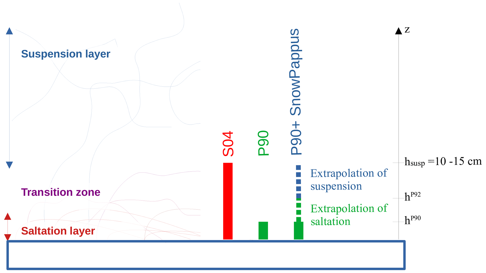
Figure 1 Schematic representation of the suspension and saltation layers and of the transition zone between them. The fluxes computed by the two saltation models S04 and P90 are represented schematically, as well as the “P90 + SnowPappus” method, combining the P90 saltation model and the SnowPappus suspension model.

Most blowing-snow models finally alter snow saltation fluxes considering the increasing relationship between flux and fetch distance (Pomeroy et al., 1993; Liston and Sturm, 1998; Bowling et al., 2004; Marsh et al., 2020). We follow this literature and use the parameterization proposed in SnowTran3D (Liston and Sturm, 1998). We consider ${\mathit{Q}}_{\inf }^{*}={\mathit{Q}}_{\inf }f\left(l_{\mathrm{fetch}}\right)$ and $c_{\mathrm{salt}}=f\left(l_{\mathrm{fetch}}\right)c_{\mathrm{salt}}^{\mathrm{P}\mathrm{90}}$ with $f\left(l_{\mathrm{fetch}}\right)=(\mathrm{1}-\exp (-\mathrm{3}\frac{l_{\mathrm{fetch}}}{l^{*}}\left)\right)$. $l^{*}=\mathrm{500}$ m represents the fetch length at which the saltation flux reaches 95 % of its steady-state value (Pomeroy et al., 1993).

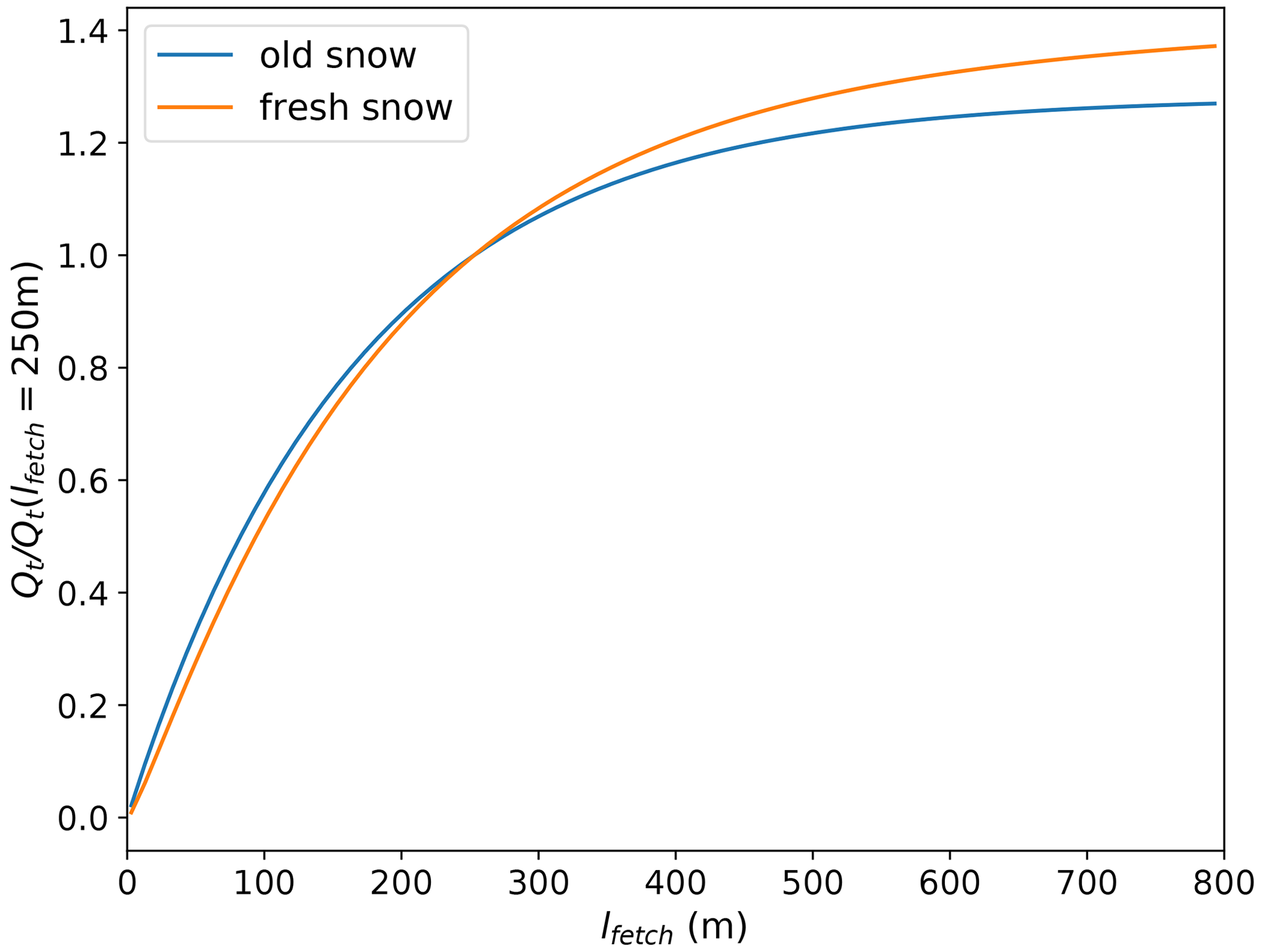
Figure 2 Ratio between the total modelled transport rate Q_t and its value for the default fetch value l_fetch=250 m as a function of fetch distance. The cases of fresh snow, i.e. dendritic snow with $u_{\mathrm{t}}^{*}=\mathrm{0.27}$ m s⁻¹ (orange curve), and old snow, i.e. non-dendritic snow with $u_{\mathrm{t}}^{*}=\mathrm{0.39}$ m s⁻¹ (blue curve), are compared, both for a wind friction velocity of 0.6 m s⁻¹ (which approximately corresponds to a 2 m wind speed of 12 m s⁻¹).

Figure 2 shows the influence l_fetch has on the total transport flux, which is very strong in the first hundreds of metres. In a mountainous environment, we can expect the typical fetch distance to be in this range and mostly lower than our resolution (250 m). For simplicity we chose to use by default a constant fetch distance on the whole grid of l_fetch=250 m, which is a strong hypothesis. Different methods and algorithms exist to compute fetch in complex topographies (Bowling et al., 2004; Marsh et al., 2020) and could be included in a future version of SnowPappus.

3.4 Sublimation

Two different parameterizations of blowing-snow sublimation rate q_subl (kg m⁻² s⁻¹) were implemented in SnowPappus with the default choice of the simplified blowing-snow model (SBSM) parameterization (Essery et al., 1999).

The first is an implementation of the SBSM parameterization from Eq. (6) of Essery et al. (1999) and the SBSM (2022) documentation:

$$\begin{array}{}\text{(18)}& {\displaystyle }{q}_{\mathrm{subl}}={\displaystyle \frac{{\mathit{\mu }}_{\mathrm{satc}}\times \mathrm{137.6}}{F\left(T\right)}}\times {\displaystyle \frac{{U_{\mathrm{10}\mathrm{m}}}^{\mathrm{5}}}{\mathrm{25}\mathrm{000}}},\end{array}$$

with the F(T) expression given in Appendix C, μ_satc the undersaturation, U_10 m the 10 m wind speed (m s⁻¹) and T the air temperature (K).

The second is from Eq. (9) of Gordon et al. (2006) is

$$\begin{array}{}\text{(19)}& {\displaystyle }{q}_{\mathrm{subl}}=A{\left({\displaystyle \frac{T_{\mathrm{0}}}{T}}\right)}^{\mathrm{4}}{U}_{\mathrm{t}}{\mathit{\rho }}_{\mathrm{a}}{q}_{\mathrm{si}}{\mathit{\mu }}_{\mathrm{satc}}{\left({\displaystyle \frac{U}{U_{\mathrm{t}}}}\right)}^B,\text{ for }U>U_{\mathrm{t}},\end{array}$$

with q_si the saturation specific humidity, ρ_a (kg m⁻³) the air density, U and U_t (m) the wind and 5 m wind threshold for transport, A=0.0018, and B=3.6.

3.5 Mass balance

This section describes how SnowPappus simulates mass exchanges between neighbouring grid cells once the amount of horizontal transport flux has been computed for each pixel. The snow transport direction is the same as the wind direction. Therefore, the problem simplifies as solving the mass balance equation. We define ${\mathit{Q}}_{\mathrm{t}}={\mathit{Q}}_{\text{inf}}+{\mathit{Q}}_{\text{susp}}$ as the total vertically integrated horizontal blowing-snow flux (kg m⁻¹ s⁻¹). The mass balance can be solved using the following continuity equation:

$$\begin{array}{}\text{(20)}& q_{\mathrm{dep}}(x,y,t)=\mathbf{\nabla }.{\mathit{Q}}_{\mathrm{t}}(x,y,t)-q_{\mathrm{subl}}(x,y,t),\end{array}$$

with q_dep (kg m⁻² s⁻¹) the pixel snow deposition, q_subl (kg m⁻² s⁻¹) the snow transport sublimation and ∇.Q_t the total snow transport flux divergence. All these quantities are expressed by sloping snow surface units. Indeed, Within the SURFEX grid configuration, each grid point has a defined slope angle θ, and each grid cell is considered to have a ground surface $\frac{l_{\text{res}}^{\mathrm{2}}}{\cos \left(\mathit{\theta }\right)}$ with l_res the grid horizontal resolution (m). In order to preserve mass balance of the domain, at a given point we assume

$$\begin{array}{}\text{(21)}& \begin{array}{rl}\mathbf{\nabla }.{\mathit{Q}}_{\mathrm{t}}& =(\mathbf{\nabla }.{\mathit{Q}}_{\mathrm{t}}{)}_{\mathrm{flat}}\cos (\mathit{\theta })=\left(\sum _{\mathrm{faces}}{\displaystyle \frac{Q_{\mathrm{t},\mathrm{in}}(x,y,t)}{l_{\text{res}}}}\right.\\ & \left.-\sum _{\mathrm{faces}}{\displaystyle \frac{Q_{\mathrm{t},\mathrm{out}}(x,y,t)}{l_{\text{res}}}}\right)\cos \left(\mathit{\theta }\right),\end{array}\end{array}$$

with (∇.Q_t)_flat the flux divergence computed as it would be on a perfectly flat terrain (kg m s⁻²).

(∇.Q_t)_flat can be expressed as the sum of the total snow transport flux Q_t leaving and entering the grid cell (in and out) by surface unit. The SnowPappus model uses a regular Cartesian mesh grid discretization with cell-centred storage. This means each simulation point is regularly dispersed on the simulation zone with each simulation point representing a squared pixel of fixed size. Our mesh grid being cell-centred, we do not compute the transport fluxes at the pixel faces, as needed for the continuity equation (Eq. 21). To obtain these values, an upwind scheme (Patankar, 2018) has been implemented; i.e. the zonal and meridian components of the fluxes at the face are assumed to be equal to the zonal and meridian flux computed at the centre of the upwind pixels (in both directions):

$$\begin{array}{}\text{(22)}& {\mathit{Q}}_{\mathrm{t}}(i,j,t)={\mathit{Q}}_{\mathrm{t}}\left(i\pm {\displaystyle \frac{\mathrm{1}}{\mathrm{2}}},j\pm {\displaystyle \frac{\mathrm{1}}{\mathrm{2}}},t\right),\end{array}$$

with i and j being the grid coordinates of the centre of pixels and $i\pm \frac{\mathrm{1}}{\mathrm{2}}$ and $j\pm \frac{\mathrm{1}}{\mathrm{2}}$ the pixel's border, as illustrated by Fig. 3.

This scheme was preferred to a linear interpolation of fluxes because it simplifies the mass balance closure in preventing snow mass creation. In our use case, the linear interpolation method would need extra steps with “gradient limiters” to ensure this (Greenshields and Weller, 2022). Besides, the effect of fetch on the transport flux may cause the flux to respond to the change in the wind and snowpack conditions with a lag of a few hundred metres, the same order of magnitude as a grid cell.

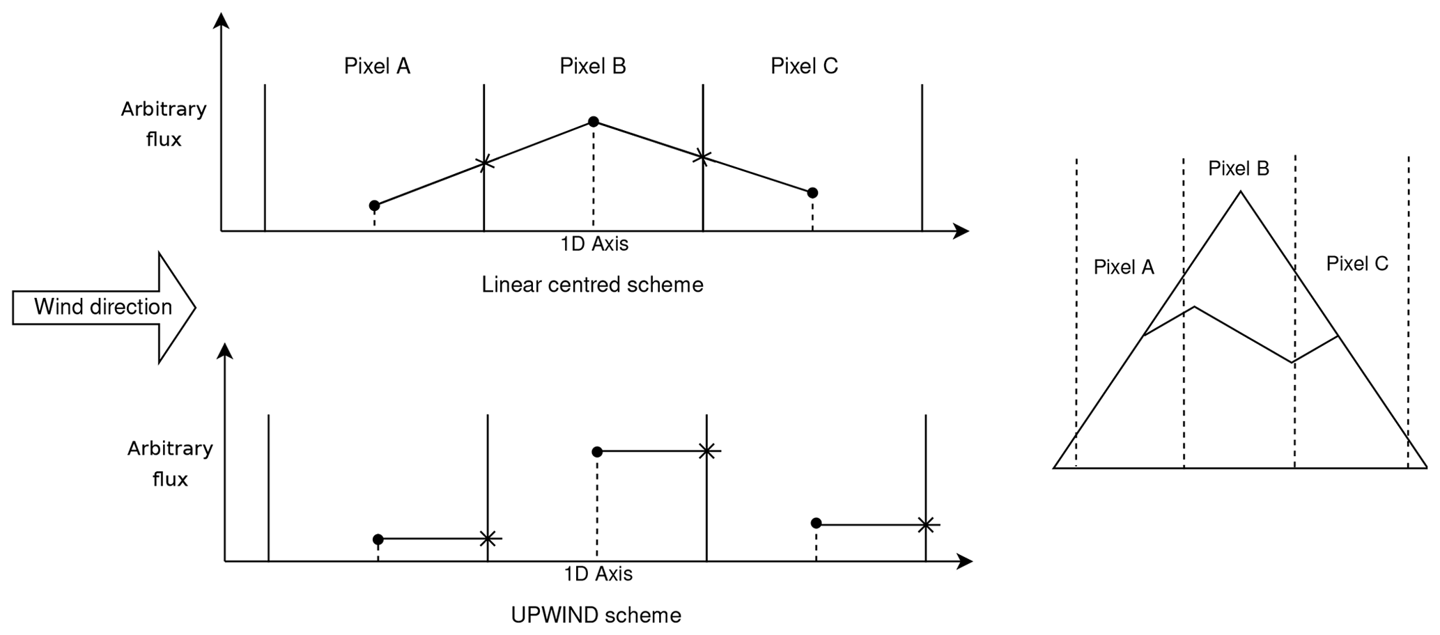
Figure 3 Illustration of the differences between the upwind scheme and a more classic linear scheme for a 1D ideal case. Dots represent the flux estimated for each pixel by in Eq. (23). Crosses (×) represent the flux value crossing the pixel face. In the linear scheme, the flux value leaving the pixel is the linear interpolation between the two-pixel cell centre values. The flux crossing the pixel face can be very different from the cell-centred computed value. The border flux being linearly interpolated, the border value can be unrealistic. This behaviour can cause interpolation to move erosion out of the expected zone (usually summits, the windiest zone). In the upwind scheme, the flux value crossing the pixel is identical to the cell-centred computed value.

We consider a given grid cell, on which local horizontal transport rate is written Q_t,out. We consider the four neighbouring cells respectively located north, south, west and east of the cell. We call Q_t,i with $i=\mathrm{1},\mathrm{\dots },\mathrm{4}$ the horizontal transport rates on these cells and call n_i the unitary normal vector going in the corresponding direction. With the upwind numerical scheme to obtain the pixel-face-crossing values, we obtain the following continuity equation for our SnowPappus model, where W_dir is the unitary vector in the wind direction (i.e. parallel to U).

$$\begin{array}{}\text{(23)}& \begin{array}{rl}(\mathbf{\nabla }.{\mathit{Q}}_{\mathrm{t}}{)}_{\mathrm{flat}}& =\sum _{i=\mathrm{1},\mathrm{\cdots },\mathrm{4}}{\displaystyle \frac{Q_{t,i}(x,y,t)}{l_{\text{res}}}}min({\mathit{W}}_{\mathrm{dir}}.{\mathit{n}}_i,\mathrm{0})\\ & -\sum _{i=\mathrm{1},\mathrm{\cdots },\mathrm{4}}{\displaystyle \frac{Q_{t,\mathrm{out}}(x,y,t)}{l_{\text{res}}}}max({\mathit{W}}_{\mathrm{dir}}.{\mathit{n}}_i,\mathrm{0})\end{array}\end{array}$$

(∇.Q_t)_flat was defined in Eq. (21), with $min({\mathit{W}}_{\mathrm{dir}}.{\mathit{n}}_i,\mathrm{0})$ and $max({\mathit{W}}_{\mathrm{dir}}.{\mathit{n}}_i,\mathrm{0})$ respectively giving the flux direction coefficient (same as wind direction) crossing each face normally for the in and out direction.

The code implementation of Eq. (23) is explained in more detail in Sect. 3.7.

3.6 Influence of snow transport and deposition on snow surface properties

As, despite qualitative knowledge of the processes, almost no observation-based parameterization of the influence of snow transport on snow surface properties (Comola et al., 2017; Mott et al., 2018; Amory et al., 2021) is available in the literature, only the following simple considerations were implemented in SnowPappus to represent it.

• Snow deposited by a transport event (when q_dep>0) has the properties of rounded grains with sphericity s=1 and dendricity d=0, as well as relatively high density ρ=250 kg m⁻³.

• Wind-induced metamorphism might also either originate from subgrid snow transport or horizontal displacement of snow with erosion and deposition flux compensating for each other. Thus, the preexisting parameterization for wind-induced snow metamorphism from Vionnet et al. (2012) can still be activated, but considering the SnowPappus threshold wind speed instead of the original formulation. It makes the surface snow layers slowly become denser and evolve towards small rounded grains approximately linearly with time. The impact is tested in Sect. 4.3

3.7 Implementation in SURFEX

SnowPappus is implemented inside the SURFEX/ISBA land surface scheme, which computes the evolution of soil and snow properties sequentially. Distributed hardware and needs of communication among grid cells require the use of the MPI protocol (Clarke et al., 1994) to be able to run distributed simulations over large domains in a short time.

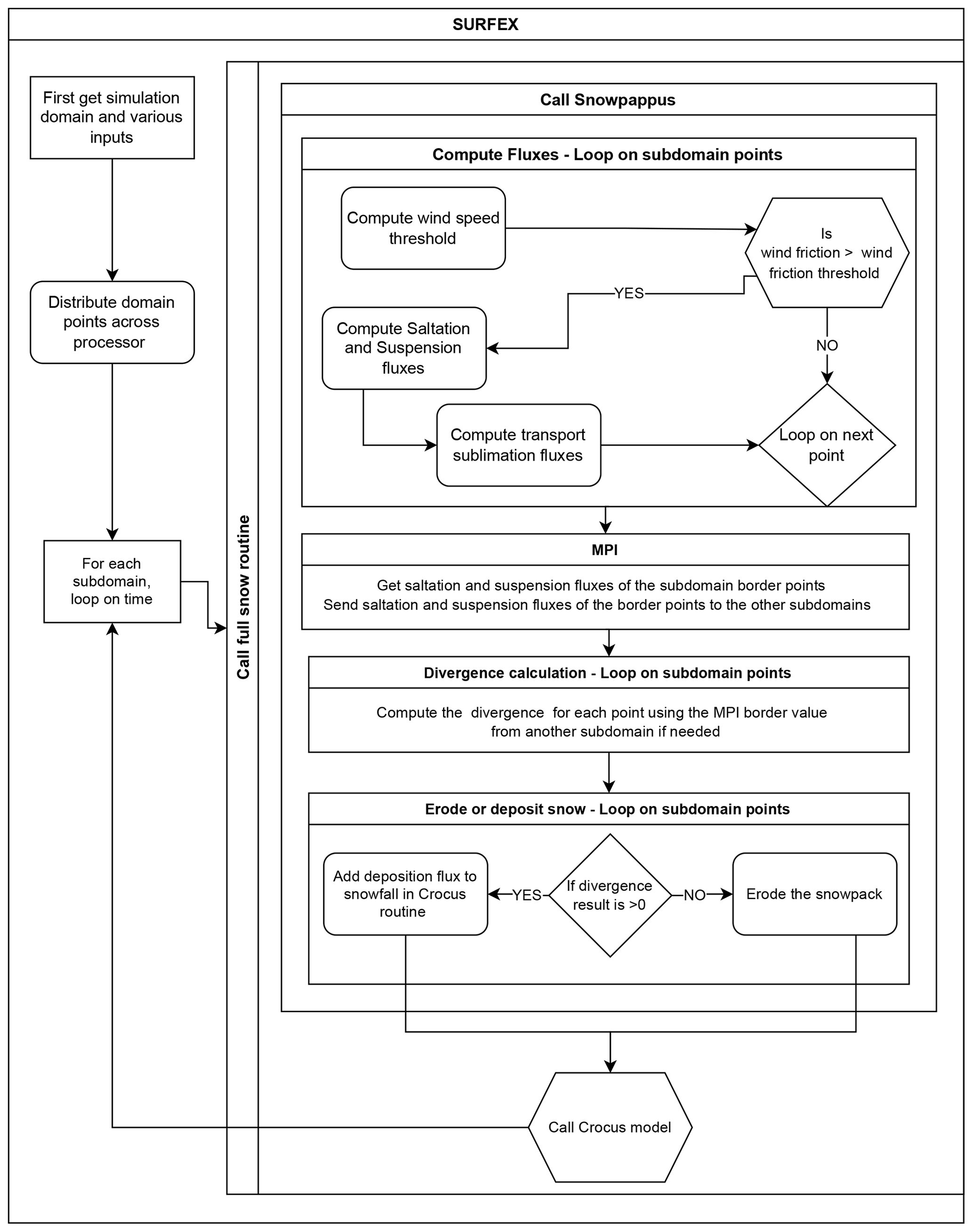
Figure 4 Description of how the SnowPappus routine is organized in the SURFEX framework and how it connects with the Crocus snow model.

At the beginning of a new simulation, an unpublished domain decomposition already implemented in SURFEX is applied to split the domain into subdomain stripes. The algorithm is designed to balance as much as possible the number of grid cells between the different cores, but all the points with the same zonal coordinate are always gathered on the same core. Therefore, the maximum number of subdomain stripes for an experiment is the number of lines of the domain. Each subdomain is associated with an MPI thread.

For each time step and subdomain, the SnowPappus routine is called before each iteration of the snowpack scheme. It computes the horizontal transport rate, Q_t, and the blowing-snow sublimation rate, q_subl, for each grid point, according to the surface properties computed in the previous time step. Then, once Q_t and q_subl are computed for all pixels, this information is shared with the processors associated with the adjacent grid point by a blocking MPI communication. After this phase, the erosion–deposition rate can be computed with Eq. (23) and converted into an amount of snow to remove or add to the snowpack. If there is net erosion, snow is directly removed in the SnowPappus routine. Otherwise, the falling snow amount and properties are computed in the SnowPappus routine and then given as snowfall input to the Crocus snow scheme.

The Crocus routine is called after SnowPappus. It deals with adding snow to the snowpack and modifying snow layers according to snowfall and SnowPappus outputs. If snowfall and wind-driven snow deposition occur simultaneously, the amount of added snow is the sum of the two. Its density and microstructure variables are a weighted average of falling snow and blowing-snow properties. The detailed equations for this process are described in Appendix E. The Crocus routine then takes back the original Crocus model course and makes the properties of snow evolve through metamorphism, heat diffusion, compaction and percolation. Those processes are summarized in Fig. 4.

It is important to note that transport rate and snowpack evolution are solved in a decoupled mode (one after the other). Therefore, the deposition rate q_dep is computed independently from the amount of snow available on the considered grid point, which can make the amount of snow removed from the point higher than the available snow mass. In this case, the mass balance is not respected. The cumulative amount of this “ghost snow” is stored in a variable to check that it remains small. To prevent this behaviour from occurring, limitations on Q_t and q_subl are made. The condition is the following:

$$\begin{array}{ll}{\displaystyle }{q}_{\mathrm{subl}}& {\displaystyle }\le {\displaystyle \frac{W}{t_{\mathrm{step}}}}\\ {\displaystyle }{\mathit{Q}}_{\mathrm{t}}& {\displaystyle }\le \left({\displaystyle \frac{W}{t_{\mathrm{step}}}}-q_{\mathrm{subl}}\right){\displaystyle \frac{l_{\text{res}}}{\cos \left(\mathit{\theta }\right)}},\end{array}$$

with W being the snow mass for each pixel in kg m⁻² and t_step the computation time step (s).

4 Evaluation: methods

4.1 Study area

For demonstration and evaluation purposes, we run simulations over a test zone covering the whole Grandes Rousses massif in the French Alps with a spatial resolution of 250 m. It covers 14 443 grid points (900 km²). This area exhibits a complex topography, with elevation ranging from 700 to more than 3500 m, involving a large range of temperature conditions and snow coverage duration. For this test zone, most winter storms come from north-western flows. Besides, to demonstrate the ability of SnowPappus to be run over large domains, we also set up a simulation domain containing the whole French Alps with about 868 000 simulation points. Both domains are illustrated in Fig. 5

4.2 Meteorological forcing

The Crocus snow model needs various atmospheric forcing variables: liquid and solid precipitation, incoming shortwave and longwave radiation, air temperature and humidity, and wind speed and direction. In this work, all these variables but the wind are given by the SAFRAN reanalysis (Vernay et al., 2022) over geographical units called “massifs” of about 1000 km² in which meteorological conditions only depend on elevation at a vertical resolution of 300 m. Here, all meteorological variables are interpolated on a 250 m resolution simulation grid, at the exact elevation of each grid point, derived from a DEM at this resolution (as in Revuelto et al., 2018, and Deschamps-Berger et al., 2022). The DEM was created by averaging on each grid point the 5 m resolution RGE Alti^® DEM provided by the Institut Geographique National at the scale of France. Snow transport modelling is strongly sensitive to the quality of the wind forcing (Musselman et al., 2015). Consequently wind fields taking into account the effect of local topographic features were preferred to the very large-scale SAFRAN wind fields. Here, kilometre-scale wind fields are first extracted from the AROME NWP model at a 1.3 km resolution (Seity et al., 2011; Brousseau et al., 2016), downscaled at a 30 m resolution using the DEVINE downscaling method (Le Toumelin et al., 2022) and finally resampled at 250 m using a simple average. The DEVINE method benefits from the use of convolutional neural networks to downscale winds from AROME to high-resolution local topography based on preliminary training with wind speeds simulated with the ARPS atmospheric model (Xue et al., 2000). Previous evaluations of DEVINE have shown that, contrary to basic wind interpolation methods, DEVINE is able to improve wind speed estimations compared to raw NWP model outputs and to reproduce several characteristics of terrain-forced flow (speed-up on crests, windward deceleration, channelling through gaps and passes) prone to influence drifting snow episodes.

4.3 Evaluation data

Blowing-snow flux data are available for three stations in the Grandes Rousses test zone. One of these is the Col du Lac Blanc observatory where long-term monitoring of blowing-snow fluxes and of various atmospheric forcings has been performed (Guyomarc'h et al., 2019). In particular, a vertical profile of snow particle counters (SPCs) (Sato et al., 1993) recording blowing-snow fluxes at four different heights is located at a particularly wind-exposed location. An estimate of vertically integrated flux between 0.2 and 1.2 m above the snow surface has been provided from these measurements from 1 December to 1 April since 2010 (Guyomarc'h et al., 2019). We use these data to evaluate blowing-snow occurrence and fluxes.

The other sites are the Huez (FHUE) and Chambon (FCMB) stations of the ISAW network already used in blowing-snow studies (Vionnet et al., 2018; He and Ohara, 2017). They are equipped with snow height, temperature and wind measurements as well as Flowcapt sensors (Chritin et al., 1999), which record integrated blowing snow from 0 to 2 m above the ground surface. Trouvilliez et al. (2015) indicate that Flowcapt sensors of different generations give similar results with respect to SPC if a threshold value higher than 1 g m⁻² s⁻¹ is taken. However, they can be partially buried under snow depending on snow height, and their reliability in terms of estimated flux is still debated in the literature (Cierco et al., 2007; Trouvilliez et al., 2015; Vionnet et al., 2018). Thus, similarly to Vionnet et al. (2018), we use them only to evaluate the blowing-snow occurrence. Flowcapt data available from ISAW stations were specifically cleaned up as described in Vionnet et al. (2018) (Sect. 3.1).

In complement to these direct transport measurements, which are available only for a few sites, we used a snow height map derived from Pleiades stereo-images (Deschamps-Berger et al., 2020; Marti et al., 2016). It is obtained as the difference between two surface elevation models computed with Pleiades data, one during a snow-free period (end of summer) and the other in winter (16 March 2018). The Pleiades snow depth map includes a few no-data areas, where the quality of observations is lower. In addition, we filtered unrealistic values out of the [−0.5 m; 20 m] range. Negative snow heights are kept as removing them would slightly positively bias the averages. This map is approximately 2 m resolution and covers an area of 168 km², shown in Fig. 5b . In order to be compared with our simulations, it was resampled to 250 m resolution as in Deschamps-Berger et al. (2022). The entire 250 m pixel is set to no data if more than 70 % of the 2 m pixels have no data. According to previous Pleiades snow map evaluations (Deschamps-Berger et al., 2020), snow height standard error can be estimated between 0.3 and 0.4 m at this resolution.

4.4 Point-scale evaluations

4.4.1 Local simulation set-ups

The accuracy of wind forcing is known to have a major influence on any evaluation of a snow transport model (Vionnet et al., 2018). Consequently, we first run and evaluate local-scale simulations at Col du Lac Blanc forced by observed 5 m wind speed in order to distinguish the contributions of wind speed errors and model errors to our results. Wind speed sensors as well as SPCs are located on the same mast at the station AWS Col described in Guyomarc'h et al. (2019). Their height above the surface is variable and recorded continuously, allowing for the estimation of 5 m wind speed assuming a logarithmic wind profile and a roughness length z₀=2.3 mm. The other meteorological variables are interpolated from SAFRAN reanalysis as for 2D simulations. In this configuration, blowing-snow fluxes are computed by the model but do not result in any erosion or deposition. These local simulations were performed from 1 August 2010 to 1 August 2020 with a soil temperature initialized by a spin-up from 2000 to 2010. At Col du Lac Blanc, fetch distance in the mean wind direction as defined in Sect. 3.3.1 was estimated to be 110±20 m, as the mean distance between the SPC sensors and the centre of accumulation zones identified from Vionnet (2012, Fig. 4.24). We thus fixed l_fetch=110 m in the blowing-snow flux simulations.

Several model configurations were used to investigate the simulated blowing-snow occurrence and are described here.

• SnowPappus: Run A. This is the SnowPappus default configuration with wind-induced snow metamorphism deactivated (see Sect. 3.6). The GM98 option is used for threshold wind speed (see Sect. 3.2).

• SnowPappus: Run B. This is the SnowPappus default configuration with wind-induced snow metamorphism activated.

• SnowPappus: Run C. This is SnowPappus with the CONS option (see Sect. 3.2), with 5 m threshold wind speed equal to 9 m s⁻¹ for snow older than 1 h. Note that the 9 m s⁻¹ was calibrated to provide the optimal Heidke skill score (see in Sect. 4.4.2) among different tested values (not shown).

• Vionnet2013. This is SnowPappus with parameters putting it in the exact same configuration as Vionnet et al. (2013) for wind speed threshold calculation and falling snow properties (see Sect. 3.2).

Additionally, to investigate the sensitivity of the simulated fluxes of blowing snow to d_m (Sect. 3.3.1), we tested three modified configurations of the Run B configuration with d_m values of 0, 0.5 and 1.

4.4.2 Evaluation of blowing-snow occurrence

We evaluate the blowing-snow occurrence using the same framework as Vionnet et al. (2018), allowing comparisons with the SYTRON operational system, which can be considered a benchmark. Contrary to SnowPappus, Sytron is based on an eight-aspect idealized geometry (Vionnet et al., 2018). Both systems share the Guyomarc'h and Mérindol (1998) parameterization for threshold wind speed calculation. As in Vionnet et al. (2018), we consider blowing snow to be observed if the blowing-snow flux measured by the SPC and integrated between 0.2 and 1.2 m exceeded a threshold of 1 g m⁻¹ s⁻¹ and simulated if a non-zero blowing-snow flux was simulated, and we define blowing-snow days as days with more than 4 h (consecutive) of blowing snow.

Here, the study was conducted for the whole 2010–2020 period, while Vionnet et al. (2018) considered only the 2015–2016 season. As in Vionnet et al. (2018), the false alarm rate (FAR), probability of detection (POD) and Heidke skill score (HSS) are used to evaluate the different set-ups:

$$\begin{array}{}\text{(24)}& {\displaystyle }\mathrm{POD}& {\displaystyle }={\displaystyle \frac{a}{a+c}},\text{(25)}& {\displaystyle }\mathrm{FAR}& {\displaystyle }={\displaystyle \frac{b}{a+b}},\text{(26)}& {\displaystyle }\mathrm{HSS}& {\displaystyle }={\displaystyle \frac{\mathrm{2}(ad-bc)}{(a+c)(c+d)+(a+b)(b+d)}},\end{array}$$

with a, b, c and d being the number of true positive, false positive, false negative and true negative events, respectively. HSS varies between −1 and +1, with +1 for perfect agreement and 0 for a random forecast.

These scores were first applied to the four model configurations previously described and to new runs of the SYTRON system to cover the same evaluation period and share the same code version of SURFEX–Crocus. For Sytron, as in Vionnet et al. (2018) (although not mentioned in the original publication), the occurrence of blowing snow is considered detected if a non-zero flux is simulated for at least one of the eight slope aspects.

The occurrence scores are then applied to the 2D simulation outputs for the 2018–2019 season, driven by simulated wind fields as described in Sect. 4.1. The evaluation is carried out at Col du Lac Blanc station and at both ISAW stations. Each station was associated with the closest grid point from its location.

4.4.3 Evaluation of blowing-snow fluxes

Integrated blowing-snow fluxes between $z_{min}=\mathrm{0.2}$ m and $z_{max}=\mathrm{1.2}$ m, called Q_t,int, were evaluated against SPC data. Modelled flux is computed at each time step by integrating suspension fluxes between z_min and z_max as in Eq. (13).

Note that the blowing-snow flux below 20 cm in height cannot be accounted for in this evaluation, although it may represent a significant contribution to the total flux. Observed data are available with a 10 min time step. For evaluation purposes, model output and SPC fluxes were first averaged hourly. As the observed fluxes cannot be used when precipitating particles prevail, periods when at least one “mean” concentration profile was observed were removed. Considering the other missing data, 4947 h of data are considered in the evaluation.

To assess the ability of SnowPappus to capture the long-term magnitude of wind-induced snow transport, monthly averages of simulated fluxes were compared to the observed ones, keeping only the months when at least 15 d of valid observed data are available. Hourly data were also classified distinguishing two cases: (i) days with snowfall according to SAFRAN reanalysis and (ii) days with no snowfall. Observation-derived wind friction velocity was also classified in 20 equally distant wind speed intervals (interval widths are about 0.064 m s⁻¹). Averaged observed and modelled fluxes by category and wind speed step were computed and compared. Less than 20 h of data were available by wind steps for $u_{*}>$0.95 m s⁻¹, so these wind speeds were not considered.

These scores were applied to the three variants of Run B configuration (three values of d_m).

4.5 2D evaluations

For sensitivity analysis and 2D evaluations, three two-dimensional simulations with different model configurations were run on the Grandes Rousses test zone.

• CTRL: SnowPappus is deactivated.

• TRANS: SnowPappus is activated with the “default” configuration, including wind-induced snow metamorphism. Blowing-snow sublimation is deactivated.

• TRANS+SUBL: same as TRANS but with sublimation activated with the SBSM method (see Sect. 3.4).

They were run from 1 August 2017 at 06:00 UTC to 1 August 2019 at 06:00 UTC. Soil temperatures were initialized by a model spin-up from 1 August 2007 at 06:00 UTC to 1 August 2017 at 06:00 UTC in a similar configuration except for the wind, which also comes from SAFRAN during the spin-up period. The TRANS simulation was used for numerical performance assessment and local evaluation of the blowing-snow occurrence.

Snow height simulated on 16 March 2018 at 10:00 is compared with the Pleiades snow height map. The forest, glaciers, lakes and cities on the domain are masked for both the Pleiades observations and simulations using the mask defined in Appendix F. An additional mask of the no-data pixels in the Pleiades data is applied to the simulations.

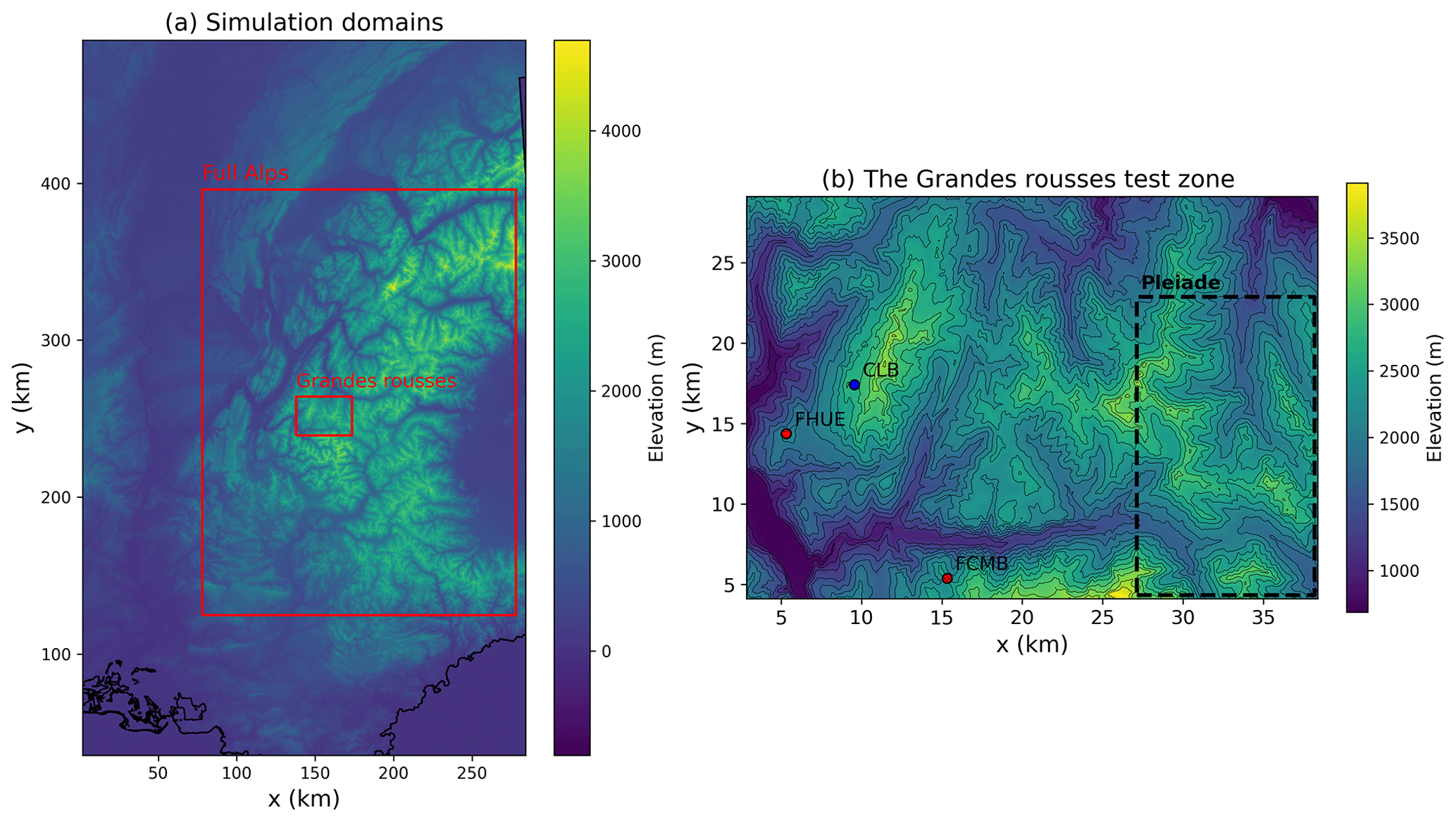
Figure 5 (a) Limits of the two domains used for simulations in the article. The small Grandes Rousses test zone is used for two-dimensional simulations presented in Sect. 5.6. The full Alps domain was used to test the possibility of running simulations on the entire French Alps (see Sect. 6.4). (b) Topographic map of the Grandes Rousses. The location of the Col du Lac Blanc experimental site (blue dot) and of the two Flowcapt sensors of the ISAW network (red dots) are indicated. The extent of the Pleiades snow depth maps is also drawn (dashed black rectangle). Equidistant iso-elevation lines are represented. Data from RGE ALTI^® were used to generate these maps.

5 Results

5.1 Comparison of saltation parameterizations

We now compare the outputs of the S04 and SnowPappus + P90 methods (see Sect. 2.2.4), which compute the blowing-snow flux up to h_susp=10–15 cm. The results of the method SnowPappus + P90 depend on the value of h_susp. Thus, we computed the blowing-snow flux with this method between 0 and 10 cm (height of the Nishimura and Hunt, 2000, experiment) and between 0 and 15 cm (height used by Melo et al., 2022, to compare S04 with their more complex saltation model). Results are presented in Fig. 6 and show that the predicted fluxes by both models give close results for friction velocities lower than 0.6 m s⁻¹. We conclude that the huge difference observed between S04 and P90 is resolved at low wind speed by adequately representing the bottom of the suspension layer, which is implicitly included in the S04 formulation. Both formulations give a flux of the same order of magnitude, and thus experimental and theoretical validations of S04 are also in agreement with SnowPappus. At high wind speed, both formulations diverge (around 0.6–0.7 m s⁻¹ for h_susp = 10 cm, 0.8–0.9 m s⁻¹ for 0–15 cm), with P90 + SnowPappus fluxes tending to curb down. This behaviour is clearly due to the fast growth of h^P92 with wind speed, making the low P90 saltation flux applied to most of the 0–15 cm layer. It must be noted that observations and simulations used for validation of the formulations are in the range 0.2–0.85 m s⁻¹ (Pomeroy and Gray, 1990; Pomeroy and Male, 1992; Nishimura and Hunt, 2000; Melo et al., 2022). Hence, both formulations might give unreasonable results at higher wind speeds. Thus, we argue both P90 and S04 give consistent results compared with other parameterizations in the literature for low to moderate wind speed.

By default, we choose to use the P90 + SnowPappus option in SnowPappus, as it gives a more coherent link between saltation and suspension and because of better empirical support of P90.

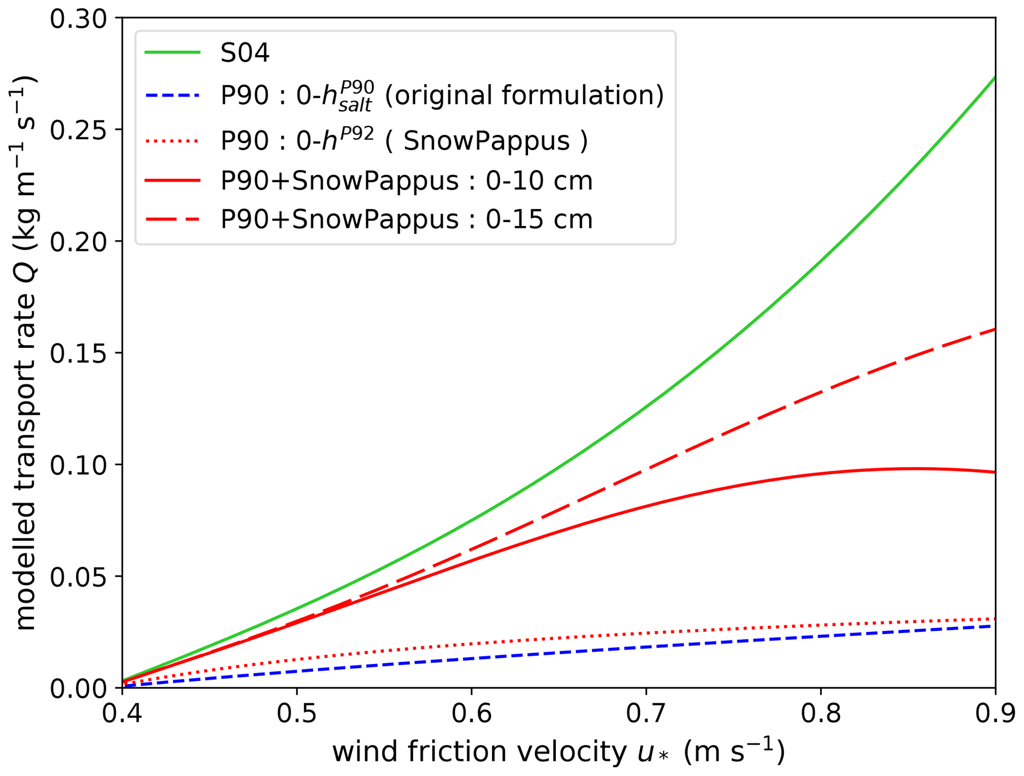
Figure 6 Comparison of the predicted flux in the saltation layer and the transition with suspension (up to 10–15 cm) with the two methods described in Sect. 2.2.5 based on P90 (blue curve) and S04 (green curve). The P90-modelled flux is computed up to (i) the integration height h^P92, which corresponds to the entire “saltation” layer; (ii) 10 cm, which is the height at which integrated measurements by Nishimura and Hunt (2000) are used to calibrate the S04 parameterization; and (iii) 15 cm, which is the height used by Melo et al. (2022) to compare S04 with a more complex saltation model, with good agreement shown (red curves). Here, all the modelled fluxes are computed for a threshold wind speed $u_{*t}=\mathrm{0.39}$ m s⁻¹, and the type of snow used in SnowPappus is old (non-dendritic).

5.2 Comparison of simulated blowing-snow flux with simple parameterizations in the literature

Before evaluating SnowPappus against observations, the relationship between Q_t and wind speed is illustrated in Fig. 7 for fresh and old snow and compared to other estimates from the literature. It stresses that, due to a lower terminal fall speed of snow particles, fresh snow exhibits much higher transport rates than old snow. The model of Essery et al. (1999) exhibits results almost identical to the “old snow” case of SnowPappus. Compared with empirical observations of Mann et al. (2000), SnowPappus transport rates simulated in both cases are in the range of the spread of observed values, at least for wind speeds lower than 20 m s⁻¹. The fresh snow case seems to approximately correspond to the upper bound of observations. These observations show that at least the magnitude of SnowPappus flux is plausible.

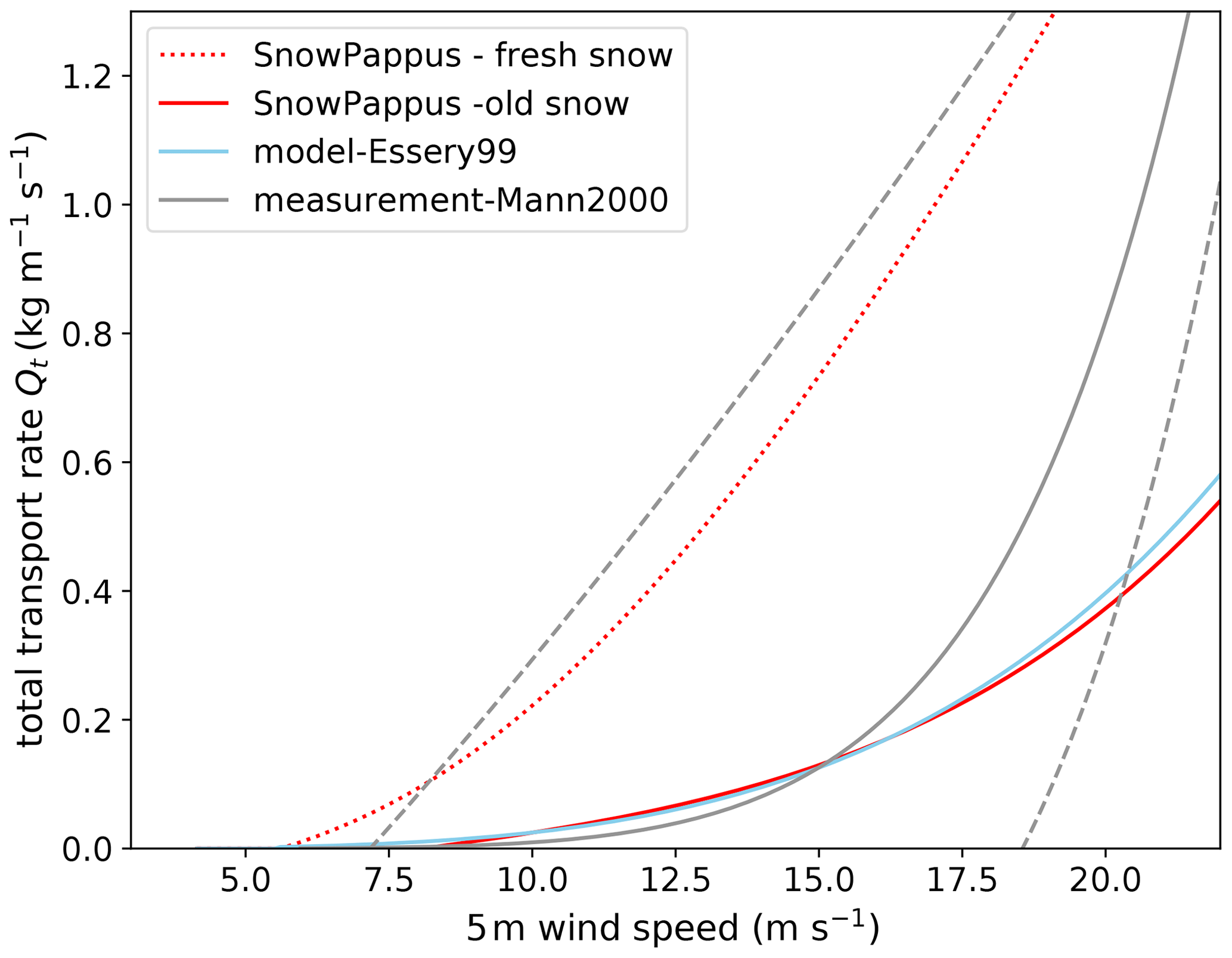
Figure 7 Total blowing-snow flux Q_t predicted by SnowPappus as a function of 5 m wind speed for old and fresh snow (red lines, see Fig. 2 for old and fresh snow discrimination). The blue line represents the flux predicted by a simplified theoretical model (Essery et al., 1999) assuming z₀=1 mm, and the grey line represents an empirical formula derived from observations in Antarctica (Mann et al., 2000) with $Q=\mathrm{1.504}{u}_{*}^{\mathrm{5.144}}$ and taking $z_{\mathrm{0}}=\mathrm{5.6}\times {\mathrm{10}}^{-\mathrm{5}}$ m $(\frac{u_{*}}{\mathrm{0.3}\mathrm{m}{\mathrm{s}}^{-\mathrm{1}}}{)}^{\mathrm{2}}$ as the authors of the studies. The dashed grey lines represent the upper and lower bounds of the observed flux, roughly estimated from Fig. 6 of the article.

5.3 Evaluation of blowing-snow occurrence at Col du Lac Blanc

HSS, FAR and POD of the different set-ups are compared in Fig. 8 for all days and for the days without snowfall. Probabilities of detection range typically from 80 % to 90 %, and false alarm rates from 30 % to 40 % considering the whole period. FAR values are higher (40 %–60 %) considering only days without snowfall.

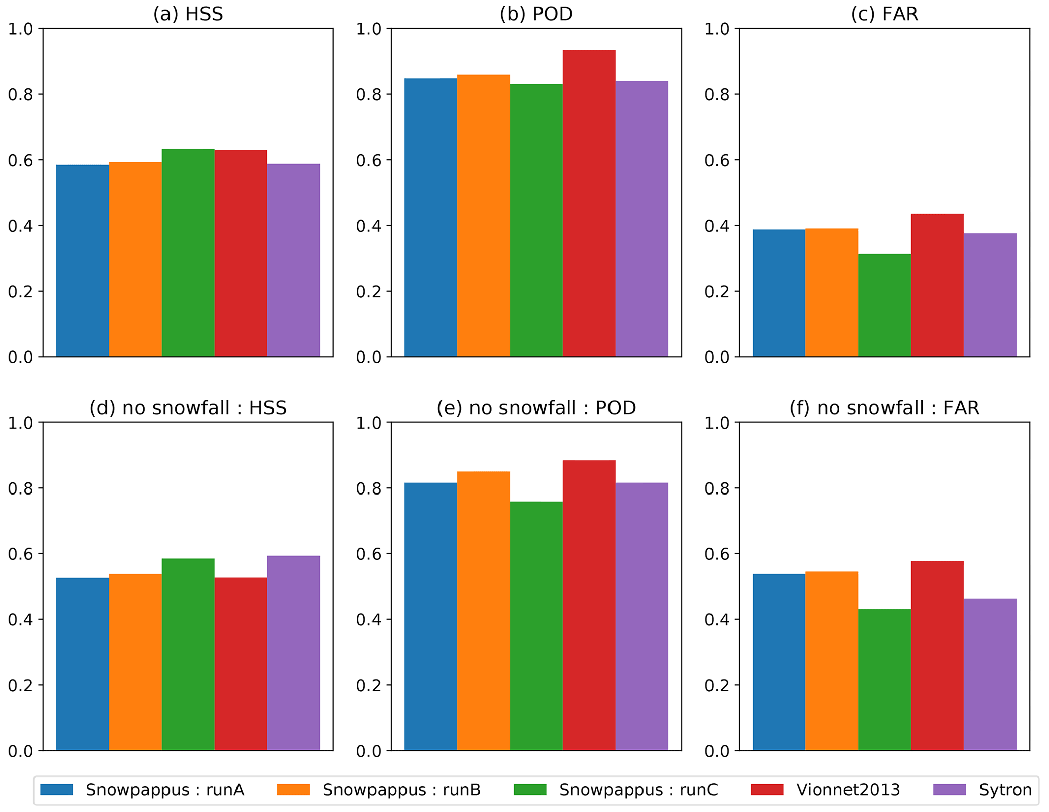
Figure 8 Evaluation of the detection of blowing-snow days with point-scale SnowPappus simulations and SYTRON operational system. HSS (a, d), POD (b, e) and FAR (c, f) of different SnowPappus configuration and other models, computed from all days independently (a, b, c) and only for days with no snowfall (d, e, f) are represented. As more detailed in Sect. 4.4.2, Run A is default SnowPappus configuration, Run B is the same with wind-induced snow metamorphism, Run C uses a constant threshold wind speed for dry snow older than 1 h and Vionnet2013 is supposed to reproduce the configuration described in Vionnet et al. (2013).

The SnowPappus default option (Run A) exhibits slightly lower FAR and POD than the approach of Vionnet et al. (2013) (Run D), which leads to similar HSS, in particular when considering only days without snowfall. Accounting for wind-induced snow metamorphism option (Run B) only slightly modifies the scores and did not improve the detection of blowing occurrence. All these methods including a threshold wind speed that depends on the properties of surface snow exhibit high false alarm rates and do not perform better than using a constant 5 m threshold wind speed in no-snowfall conditions (Run C). In addition, SnowPappus, with its different options, and the SYTRON operational model exhibit similar scores.

5.4 Evaluation of blowing-snow occurrence in 2D simulations

Scores of blowing-snow detection obtained with 2D simulations at Col du Lac Blanc, Huez and Chambon stations are shown in Fig. 9. HSS and POD are low in this configuration using wind speed downscaled at 250 m grid spacing using the DEVINE approach. At Col du Lac Blanc, the HSS is lower than the HSS obtained for point-scale simulation forced by observed wind speed. This decrease in HSS mainly results from a strong decrease in POD (Fig. 9b). It suggests that the accuracy of the downscaled wind speed and/or the 250 m spatial resolution of the simulation is the main cause of the skill deterioration, as confirmed by the significant discrepancies between observed and simulated wind speeds at the three stations (Fig. 11), with a variable skill between Col du Lac Blanc (R²=0.71, RMSE =3.3 m s⁻¹), Huez (R²=0.49, RMSE =2.5 m s⁻¹) and Chambon (R²=0.42, RMSE =3.0 m s⁻¹) stations and a significant underestimation of the highest wind speeds at all sites.

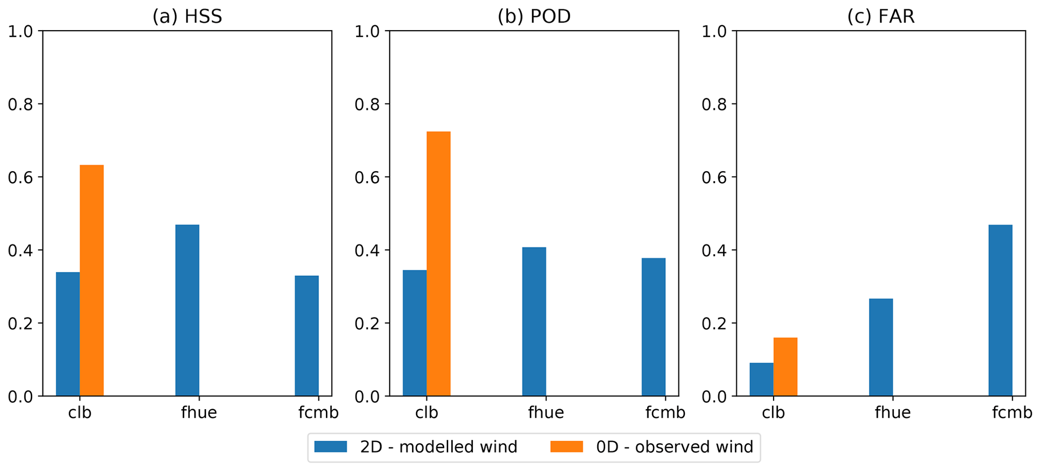
Figure 9 Blue bars: HSS, POD and FAR for the detection of blowing-snow days in 250 m resolution simulations against Flowcapt data from ISAW stations of Huez (fhue) and Chambon (fcmb) and SPC data from Col du Lac Blanc (clb). Orange bars: same scores in point-scale simulations with the same SnowPappus configuration forced by observed wind speed (Run A in Fig. 8).

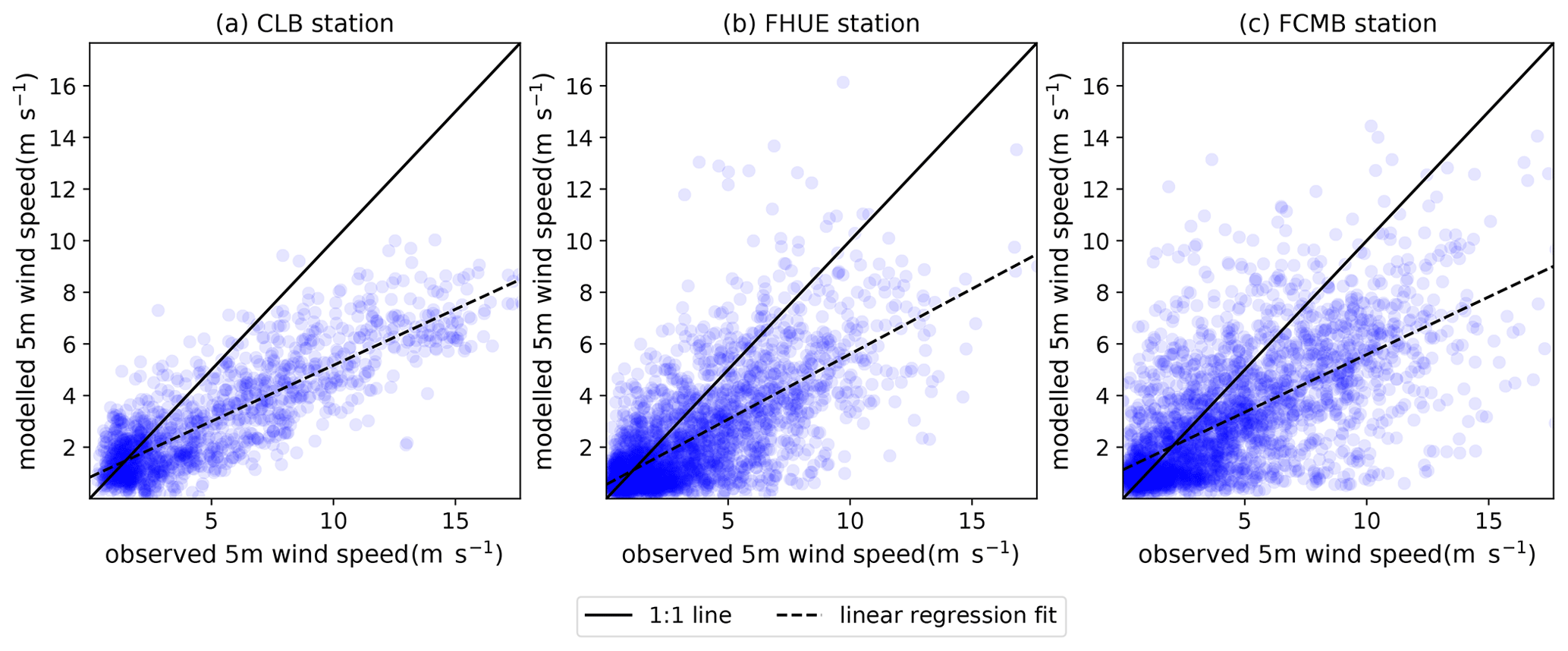
Figure 10 Comparison between observed wind at Col du Lac Blanc as well as at Huez and Chambon ISAW stations and the 250 m resolution DEVINE-modelled wind used as a forcing in the closest simulation points. Linear regression lines fitting the modelled wind as a function of the observed ones are presented. The presented points are the ones used for blowing-snow occurrence evaluation in Fig. 9. Wind observed data were filtered using the same algorithm as in Le Toumelin et al. (2022).

5.5 Evaluation of blowing-snow fluxes at Col du Lac Blanc

Figure 11a shows the simulated monthly averaged fluxes between 0.2 and 1.2 m (Q_t,int) at Col du Lac Blanc as a function of the observed ones for the three tested d_m values. As expected, fluxes clearly increase when d_m decreases because it makes the terminal fall speed closer to the fresh snow regime. Simulated Q_t,int is of the same order of magnitude as the observed one. It is clearly overestimated when d_m=0, clearly underestimated when d_m=1 and slightly underestimated when d_m=0.5. In all cases, modelled fluxes seem to correlate well with observed ones but with a strong dispersion. In particular, one specific month has a simulated flux 8 times higher than the observed one regardless of the d_m value and will be discussed in Sect. 6.1.1.

Figure 11b shows average simulated and observed fluxes as a function of the 5 m wind velocity for days with and without snowfall for wind friction velocities between 0 and 0.95 m s⁻¹. Simulated and observed fluxes show the same dependency with u_*, the flux remaining negligible under a threshold wind speed and then increasing in a steady non-linear way. Moreover, both observed and simulated fluxes are higher during days with snowfall than during days without snowfall. Therefore, we can state that SnowPappus correctly reproduces the dependency of blowing-snow flux on snow age and wind speed. In particular, the relationship between Q_t,int and wind speed is very close to the observed one in the case of d_m=0.5.

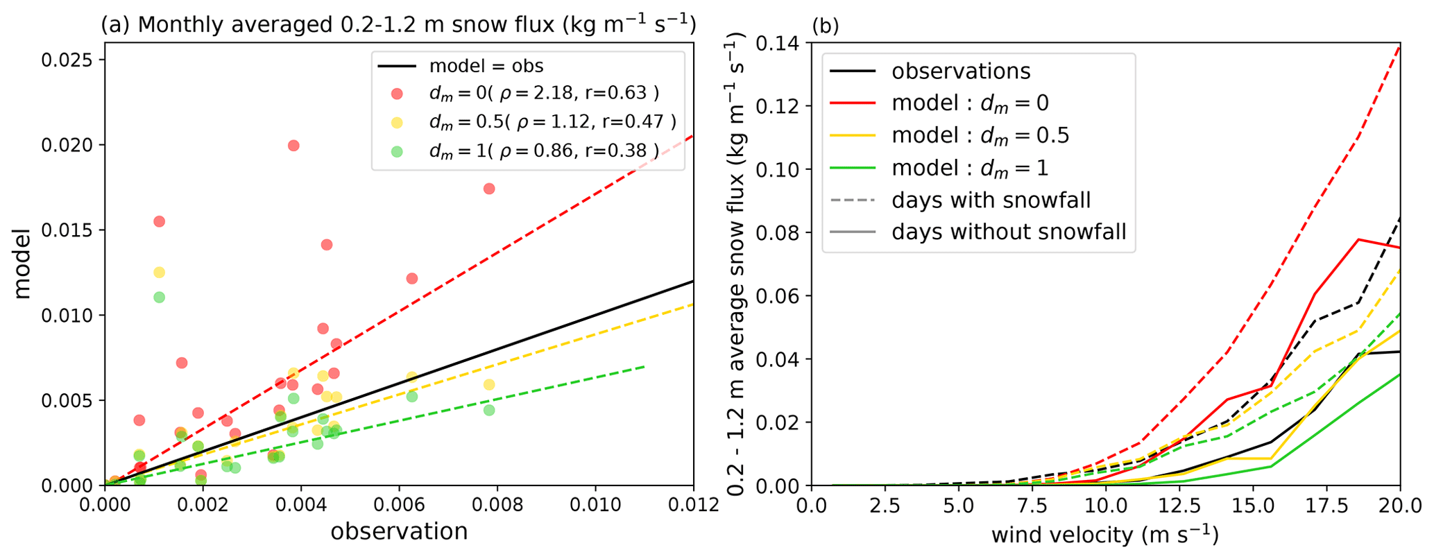
Figure 11 (a) Simulated monthly averaged Q_t,int at Col du Lac Blanc as a function of SPC-observed fluxes for three different values of d_m. The 1:1 line representing equality between the model and observations is drawn in black. The dashed lines are Theil–Sen regression fits (Wilcox, 1998) of each model configuration. Ratios of model–observation differences of total cumulated fluxes (ρ) and the correlation coefficient (r) are indicated in the legend. (b) Observed and modelled Q_t,int (with the same model configuration as (a)) averaged by 5 m wind velocity intervals as a function of the interval mean wind friction velocity. Dashed lines are computed from the data for days with snowfall and plain lines with the data for days without snowfall.

5.6 Sensitivity analysis and evaluation of 2D simulations

Comparisons of the influence of transport and blowing-snow sublimation on snow depth simulations at the end of the 2017–2018 snow accumulation season are displayed in Fig. 12. Wind-induced snow transport has a visible and spatially heterogeneous influence on snow depth at high elevations (above approximately 2500 m), but this influence remains quite weak (dozens of centimetres) except near the highest crests, where up to 2–3 m of snow ablation is simulated at the top of them, along with an equivalent accumulation zone usually on the south-east slope directly below. The sensitivity of the simulation to sublimation activation is low compared to the snow transport effect (Fig. 12b), rarely more than 10 cm.

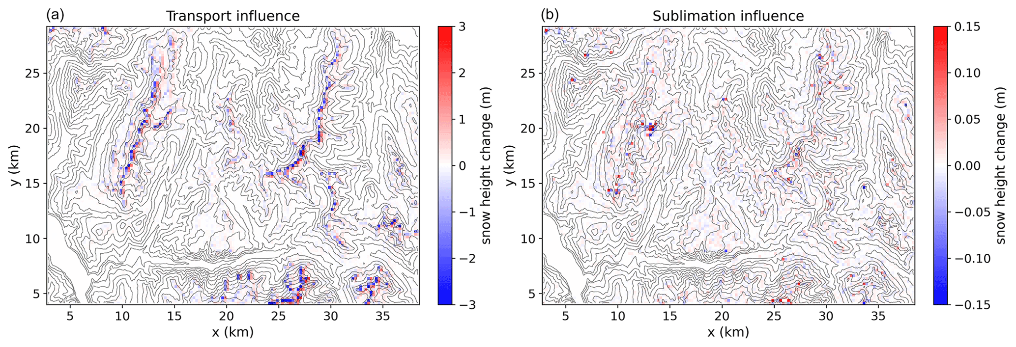
Figure 12 (a) Snow depth difference (m) between the TRANS and CTRL simulation on 16 March 2018, which approximately corresponds to the end of the accumulation season. (b) Snow depth difference (m) between TRANS+SUBL and TRANS simulations.

Then, we compare simulated snow depth maps with and without blowing-snow transport (TRANS and CTRL) with the Pleiades snow depth map. They are shown in Fig. 13. In CTRL simulations, no small-scale snow depth variability is visible, which is in clear contrast with the Pleiades image. In contrast, small-scale snow depth patterns are clearly visible at high elevation in the TRANS simulation. It makes the snow depth probability density function above 2700 m much closer to observations for the TRANS simulation, although the spatial variability is still underestimated. Visually, small-scale spatial variability is clearly higher in the Pleiades image than on modelled snow depth maps. Thus, strong regular patterns of ablation–deposition visible in the simulations are less obvious in observations. In spite of this, we can note that the location of the simulated snow ablation zone, on the top of the crests, seems to often correspond to pixels with a smaller observed snow height than the surroundings. However, the intensity of the patterns often seems misrepresented, in particular on some crest summits where simulated erosion is very strong compared with observations, which is visible in the snow height distribution. Despite these limitations, representing wind-induced snow transport significantly raises point-to-point Pearson correlations ρ between observations and simulations at high elevation. Indeed, above 2700 m, we obtain ρ_CTRL=0.12 (p value >0.05) and ρ_TRANS=0.34 (p value <0.05).

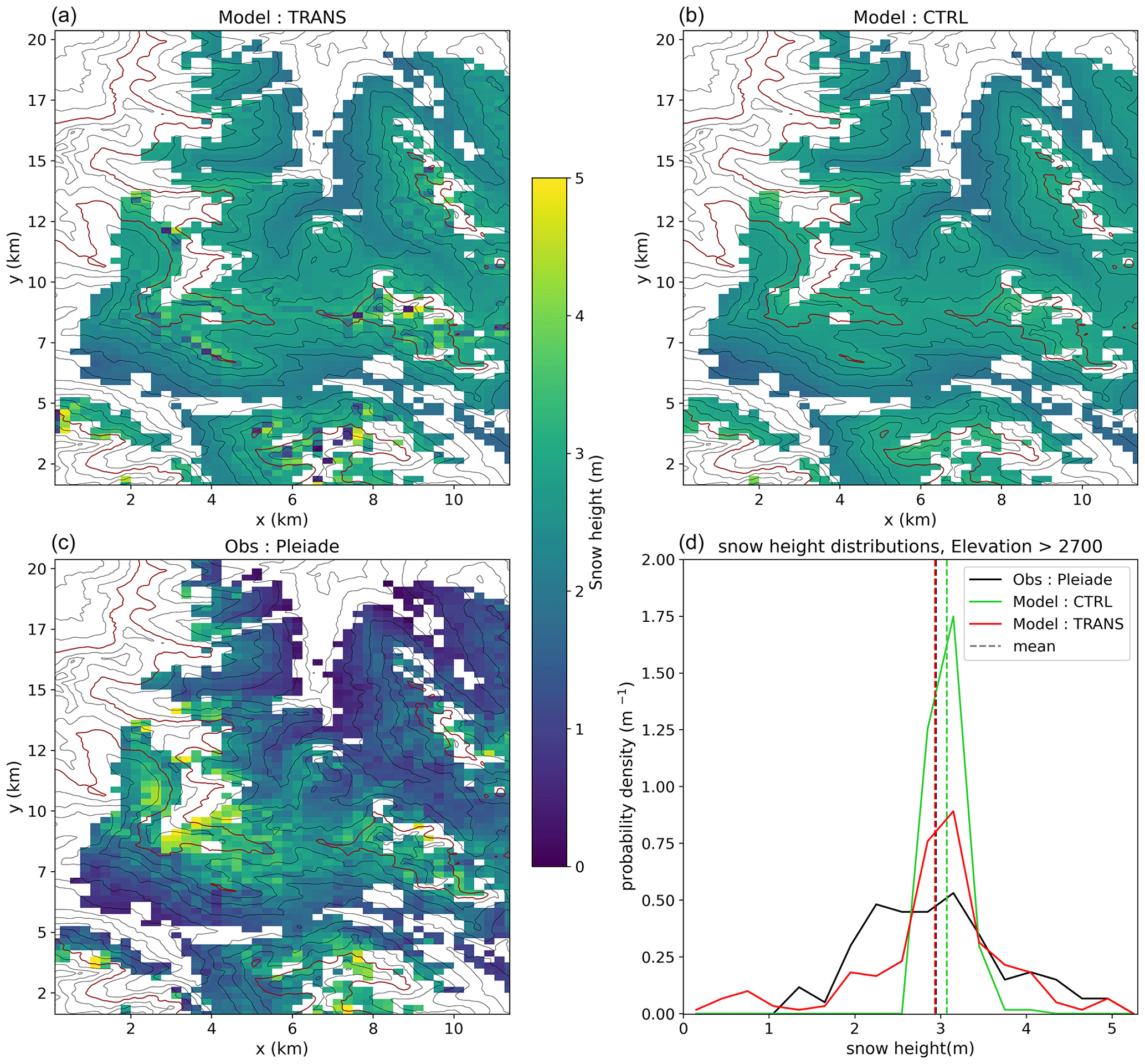
Figure 13 (a) Simulated snow depth map on 16 March 2018 at 10:00 computed with the TRANS configuration (snow transport activated) for the region covered by the Pleiades image. White pixels are those which are not included in the analysis for reasons described in Sect. 4.3. (b) Simulated snow depth map with the CTRL configuration (snow transport deactivated). (c) Observed snow depth map with stereo Pleiades imagery, resampled at 250 m resolution. (d) Probability density distributions of snow depth simulated with TRANS and CTRL configurations and observed with Pleiades. Mean snow depth is represented as dashed lines (note that Pleiades and TRANS mean snow depths are superposed). Only pixels above 2700 m are considered. The 2700 m isoline is highlighted in red in panels (a), (b) and (c).

6 Discussion

6.1 Point-scale blowing-snow flux and occurrence computations

SnowPappus model outputs depend on two major steps, which are (i) computing the local blowing-snow fluxes and (ii) computing snow redistribution among grid points. Besides, they are highly dependent on wind speed (Fig. 7). Thus, we first discuss the model skill of point-scale simulations at Col du Lac Blanc forced by observed wind speeds. It will allow us to discuss our theoretical choices and their limits in terms of blowing-snow flux computation.

6.1.1 Quality of point-scale flux prediction and comparison with other studies

Blowing-snow occurrence detection in SnowPappus and the SYTRON operational system (Vionnet et al., 2018) is based on formulations derived from the Vionnet et al. (2013) algorithm (hereafter VI13). We performed a long-term evaluation of this process within SnowPappus, VI13 and SYTRON at Col du Lac Blanc observatory for the 2010–2020 period. It can be compared to other evaluations of VI13 and SYTRON systems performed at the same site in the 2001–2011 and 2015–2016 periods, respectively (Vionnet et al., 2013, 2018). Our results show that VI13, SnowPappus and SYTRON exhibited similar scores and are coherent with the previous evaluation of VI13 in a different period. All three methods give reasonable but perfectible detection scores with a large false alarm rate, even if Vionnet et al. (2013) argued in a similar context that it may mainly concern events with very low simulated blowing-snow fluxes. However, the previous evaluation of SYTRON by Vionnet et al. (2018) showed better performances, with a perfect detection of blowing-snow events on a daily timescale at Col du Lac Blanc for one winter, which differs notably from our own SYTRON evaluation. We were able to retrieve the original simulation outputs of Vionnet et al. (2018) and applied our evaluation process to these data (see “Code and data availability”), obtaining results very close to ours. Thus, after discussion with the authors, it is clear that the issue comes from irreproducible data post-processing applied to the SPC data to compile results at the daily timescale.

In terms of fluxes, evaluation of the monthly averaged blowing-snow fluxes integrated between 0.2 and 1.2 m was performed with different parameterizations of the effective terminal fall speed $v_{\mathrm{f}}^{*}$. It shows SnowPappus is able to simulate satisfactory average fluxes at Col du Lac Blanc if $v_{\mathrm{f}}^{*}$ is adequately calibrated. However, simulated fluxes suffer from a high standard deviation of the error, leading to a low correlation between observed and simulated data. A particular outsider monthly value can be identified in Fig. 11, but, given the meteorological condition during the associated month (see Appendix Fig. A1), it probably comes from a detector failure rather than from a model overestimation. Moreover, Fig. 11a shows that the flux dependency on wind speed and snow age is correctly reproduced by SnowPappus. Overall, this point-scale evaluation of snow fluxes at Col du Lac Blanc shows that SnowPappus provides good orders of magnitude of blowing-snow suspension fluxes and occurrence when an observed wind forcing is used. However, the model exhibits a strong uncertainty at the event timescale.

A major strength of our evaluation is the long-term period encompassing 10 winter seasons, while most previous studies evaluating simulated blowing-snow fluxes in seasonal snowpack conditions only considered a few blowing-snow events taken within a period of time of typically 1 month (Pomeroy and Male, 1992; Naaim-Bouvet et al., 2010; Vionnet et al., 2014). Considering the dispersion of the monthly averaged fluxes we obtain, such short evaluations may be strongly biased. In particular, Naaim-Bouvet et al. (2010) evaluated a formulation of blowing-snow flux which is very close to ours in the case of fresh snow but assuming an infinite fetch. Contrary to us, their model overestimated the flux by an order of magnitude, which could be due to the combined effect of the infinite fetch assumption and the specificity of the two considered events. Longer-term evaluations of blowing-snow fluxes could be found in Antarctica. For example, an evaluation of the monthly averaged flux simulated by the MAR model in Antarctica was performed at two stations with 2- and 8-year time series (Amory et al., 2021). Correlation coefficients of 0.6 and 0.8 were obtained between observations and the model. The correlation we obtain is close to or lower than their results for the first station, although the results are not fully comparable (different seasonality of the fluxes, use of simulated wind speed, etc.). Qualitatively, all the mentioned studies obtained a strong dispersion of model errors which is consistent with our results.

However, the use of Flowcapt and SPC data during precipitation events for evaluation purposes is questionable. Indeed, some field evaluations suggest that the less rounded snow particle shape in these conditions leads to bias of the flux estimates (Sato et al., 2005; Trouvilliez et al., 2015). Moreover, both instruments do not distinguish blowing-snow particles from precipitating snowflakes, which by themselves can be responsible for fluxes of typically 0.1 to 10 g m⁻² s⁻¹ (Vionnet, 2012, Fig. 4.17b; Vionnet et al., 2017, Fig. 7). This may deteriorate our results for blowing-snow occurrence, as we did not take this possibility into account.

6.1.2 Sensitivity, added value and robustness of microstructure-dependent parameterizations

We performed blowing-snow suspension flux evaluations making the parameter d_m, which influences the terminal fall speed, vary within a range which is compatible with the current state of knowledge. Results show that (i) the value d_m=0.5 allows for simulations of realistic average fluxes and (ii) the value of the flux is strongly influenced by d_m, which can make its cumulative value vary by almost a factor of 3 in the explored range. d_m controls the terminal fall speed of suspended particles, so it highlights the extreme sensitivity of suspension to this parameter, which is for now imprecisely known.

On the other hand, results for the blowing-snow occurrence at Col du Lac Blanc suggest that the differences between the VI13 method and SnowPappus do not lead to significant differences in the quality of the simulations. Consequently, in the current state of knowledge, both methods can be used. Results also show that the wind-induced snow metamorphism option seems to have only a very small effect on the simulated blowing-snow occurrence. It means it might not enhance the quality of simulation in the alpine environment, although complementary evaluations of its impact on the snow stratigraphy would be required, in particular within 2D configurations of the model. Moreover, for the first time to our knowledge, we compared the results of these parameterizations based on microstructure to a much simpler one where the wind speed threshold depends only on whether or not snow was deposited less than 1 h ago. It emphasizes the fact that a well-calibrated constant threshold wind speed performs as well or even slightly better than those parameterizations.

However, considering some limits in our study, the above statements must be taken with caution. Indeed, only blowing-snow fluxes integrated between 0.2 and 1.2 m were evaluated, which ignores what happens in the saltation layer and in the saltation–suspension interface. Moreover, evaluations and calibrations of flux and occurrence were applied to only one site, with particular climate and environmental conditions. The calibrations of d_m and of the constant-threshold wind speed may be overcalibrated to this site and thus not directly valid or optimal at other sites. The absence of added value of Guyomarc'h and Mérindol (1998) at Col du Lac Blanc may indicate that it does not capture the temporal variability of threshold wind speed at this site or that simulated snow surface properties are not relevant.

6.1.3 Uncertainty in the parameterizations used

Local flux evaluation results suggest that the complexity of parameterizations, at least for suspension fluxes and blowing-snow occurrence, is not directly linked with model accuracy. Indeed, our simple suspension model exhibited a very high sensitivity to the snow particle effective terminal fall speed $v_{\mathrm{f}}^{*}$, which is also involved in more complex suspension models (Bintanja, 2000; Vionnet et al., 2014). Thus, enhancing our knowledge of this parameter and its link to snow properties may allow a larger improvement of suspension flux simulation than making the models more complex. Besides, simplification of the threshold wind speed dependency on snow properties, as well as the inclusion of wind-induced snow metamorphism, did not significantly change the blowing-snow occurrence prediction skill. It could be explained by the fact that the interest in such parameterizations can also be limited by intrinsic errors of the Crocus model in terms of surface properties. The hypothesis that a unique threshold wind speed can be used for initiation and stop of the transport in given conditions may also affect this conclusion, as well as the time step of the model, which is longer than the duration of individual continuous transport events (Doorschot et al., 2004). Consistent with our results, it must be noticed that a recent development in MAR by Amory et al. (2021), including among others a simplification of the threshold wind speed parameterization, led to an improvement of the model skill.

Finally, there are many “blind points” of the snow transport literature that limit the possibility to parameterize some phenomena which may have a strong influence. For example, we could not find any study about the influence of the slope on snow saltation transport, whereas it was shown to influence sand transport (White and Tsoar, 1998) and steep slopes are common in complex terrain. Besides, many wind-induced snow transport events occur during snowfall (Vionnet et al., 2013). However, saltation fluxes and initiation were never studied during snowfall events to the best of our knowledge, whereas snowfall obviously changes snow cohesion and properties and interacts with grain ejection mechanisms. Finally, quantitative information about the action of transport on snow surface properties is still lacking, despite some recent results on density evolution (Sommer et al., 2018; Amory et al., 2021). We think field or wind tunnel measurements of snow specific surface area (SSA) and density in snow deposition zones, as well as observations of their temporal evolution during blowing-snow events, would maybe allow testing and improving the hypothesis we had for SnowPappus development.

6.2 Use of SnowPappus in distributed simulations

6.2.1 Added value of SnowPappus in 2D simulations

Two-dimensional simulations of the Grandes Rousses test zone (see Sect. 5.6) showed that activating snow transport has a significant influence on snow height spatial distribution at high elevation at the end of accumulation season, reaching up to 2–3 m of erosion–deposition near high alpine crests. Comparable snow height differences were obtained with PBSM-3D (Vionnet et al., 2021). Moreover, comparisons with the Pleiades image show that this effect results in a qualitative and quantitative improvement of agreement between simulations and observations, with an increase in snow height variability and a moderate but significant improvement of point-to-point correlation. Thus, including wind-induced snow transport in hectometre-scale simulations seems to be promising, although strong errors remain. In particular, erosion patterns seem overestimated near crests, while overall snow spatial variability is still underestimated in simulations. These improvements and limitations are quite coherent with those observed in Vionnet et al. (2021), which is to our knowledge the only other published quantitative evaluation of simulated snow depth patterns in a full winter season blowing-snow simulation.

However, activation of blowing-snow sublimation seems to have a limited effect on simulations. Previous modelling studies in alpine terrain (Vionnet et al., 2014; Strasser et al., 2008; Sexstone et al., 2018) also found a relatively low contribution of blowing-snow sublimation, although some suggested it can have an important local impact near crests (Strasser et al., 2008; Sexstone et al., 2018).

6.2.2 Sources of uncertainty and limitations of the study

In addition to the previously discussed uncertainty in local flux simulation, distributed simulations are hampered by several other sources of uncertainty, which could explain the high remaining errors in 2D simulations with transport.

Indeed, the extent of areas strongly influenced by transport typically encompasses a few grid points. Thus, we can expect results to be hampered by strong numerical errors and discretization issues, as suggested by previous studies at 25–200 m resolution (Lehning et al., 2008; Bernhardt et al., 2009; Grünewald et al., 2010). In particular, overestimation of erosion patterns was often found above 25 m resolution (Vionnet et al., 2021; Lehning et al., 2008). Besides, low resolution makes local evaluation of a distributed model difficult at such resolution in complex terrain, as gridded meteorological forcings, in particular wind, and consequently simulated snow conditions may not be representative of local conditions observed by sensors. For example, poor results for blowing-snow occurrence were obtained when using 2D simulations, which is partly explained by the important difference between the value of this wind taken at the closest grid point and the local one.

Beyond this resolution issue, blowing-flux computation is highly sensitive to wind (e.g. Essery et al., 1999; Mann et al., 2000; Schneiderbauer and Prokop, 2011b), making it largely dependent on the quality of wind forcing, which could easily become a major limiting factor for local blowing-snow flux assessment. Moreover, it may become even more limiting for the prediction of spatial erosion and deposition patterns (Musselman et al., 2015). The improvement of wind field assessment in mountainous areas is beyond the scope of this study but has recently been investigated by several authors (Raderschall et al., 2008; Helbig et al., 2017; Dujardin and Lehning, 2022). Therefore, the possibilities for improvements in snow transport modelling depend heavily on the ongoing advances in this area.

Finally, snow depth pattern differences between the model and observations come from both a misrepresentation of wind-induced snow transport and other sources of errors. In particular, precipitation forcing at high altitudes also suffers from high uncertainty, which usually leads forcing errors to prevail in snow simulation systems that are not forced by local observations (Raleigh et al., 2015; Schlögl et al., 2016; Günther et al., 2019). A detailed sensitivity analysis of spatialized snow simulations to precipitation forcing, blowing-snow representation and model resolution is provided by Haddjeri et al. (2023). It shows that both components highly interact in any evaluation of 2D simulations and that results ignoring these uncertainties should be considered with caution. However, the added value of SnowPappus to simulate the spatial variance of snow depth and snow melt-out date at high elevations and around crests is confirmed by Haddjeri et al. (2023), with more satellite observations than the ones used in this paper.

6.3 Limits of applicability

SnowPappus development relied mostly on parameterizations inferred from observations averaged on a 7.5–10 min period and performed in environments with seasonal snowpack and at mid-latitudes (Pomeroy and Gray, 1990; Pomeroy and Male, 1992; Vionnet et al., 2012), which approximately corresponds to our goals in terms of time step and environment for our model applications. Use of these parameterizations at much smaller time steps or in very different snow conditions may result in bias. In the case of time step, these concerns are due to the fluctuating nature of wind and non-linear dependence of blowing-snow-related quantities on it. Besides, moving to much higher resolutions than 250 m or simpler topographies would possibly require a better treatment of non-local effects by explicitly taking fetch distance into account and solving a 3D advection–diffusion equation.

6.4 Applicability at large scale

The technical possibility to apply SnowPappus in large-scale simulation was one of the targets of this work. The detailed evaluation of its computing performance is provided in Appendix G and shows that the computing time of the SnowPappus physical routine is negligible compared with the one of Crocus. However, scalability issues caused by MPI communications in a highly parallel environment are an important limitation. Despite these current limitations, we were able to perform a yearly simulation on a domain covering the full French Alps (see Fig. 5) in 17 h of simulation time using only one computing node. It means daily operational simulations implying 8 d of simulations in the current French system (Morin et al., 2020b) would require only 30 min of computing time on one node, which is affordable. Therefore, the main criterion for using SnowPappus in an operational system in the near future will be our ability to demonstrate its added value in snow cover simulations rather than computation time limitations.

7 Conclusions

This paper presents SnowPappus, a new blowing-snow model coupled with the Crocus state-of-the-art snow scheme. It aims to be part of a future operational system running distributed snowpack simulations over the entire French mountains at 250 m grid spacing. SnowPappus is a simple model computing blowing-snow fluxes using semi-empirical parameterizations to represent saltation and solving suspension in a one-dimensional stationary state, like models such as PBSM (Pomeroy et al., 1993) or SnowTran3D (Liston and Sturm, 1998). It includes newer results on the terminal fall speed of snow particles (Naaim-Bouvet et al., 2010; Vionnet, 2012), which have a strong influence on the simulated snow fluxes, and a parameterization of the threshold wind speed based on Crocus-simulated microstructure properties. Several options are available to represent threshold wind speed, suspension, sublimation and wind-induced snow metamorphism. MPI parallelization handles the data sharing between neighbouring points required to compute snow redistribution on parallel computers. Performance tests show that Crocus coupled with SnowPappus is able to run a simulation over the full French Alps during an entire snow season within a reasonable computation time.

Local evaluations of suspension snow flux and blowing-snow occurrence using observed wind fields to drive SnowPappus were also performed. They show that SnowPappus is able to simulate reasonable average suspension fluxes if the effective terminal fall speed of suspended snow particles is adequately calibrated and that blowing-snow occurrence is satisfactorily captured. However, the simulation outputs have a strong uncertainty, which is coherent with previous results obtained with other models. Numerous badly known physical parameters and understudied parameters limit improvements of the parameterizations used. Moreover, uncertainty linked to parameterization is combined with uncertainties in forcing wind speed. Therefore, it may lead to local fluxes being strongly different from the simulated one. They will have to be understood more as a “first guess” than as a quantitative estimate.

Despite these uncertainties, evaluation of simulated snow depth patterns against a satellite-derived snow depth map showed a significant improvement in snow spatial variability and spatial correlation with observation. Complementary evaluations of the simulated snow spatial distribution against other satellite data confirm this conclusion in spite of the prevailing uncertainty of meteorological forcing in such a context (Haddjeri et al., 2023) (snow depth maps from satellite stereo imagery, snow cover maps for satellite optical imagery). The 250 m resolution is, however, a challenging spatial scale for snow simulations that is not able to fully solve snow transport processes. Parameterizing the effect of subgrid topography on transport fluxes (Bowling et al., 2004) would therefore be a promising way to improve the realism of simulations.

Appendix A: Supplementary figures

Figure A1 Modelled and SPC-measured 0.2–1.2 m blowing-snow flux during January 2018. SAFRAN-modelled air temperature and solid precipitation, as well as measured wind speed, are also represented. This month is a clear outlier in the comparison between observed and modelled fluxes presented in Fig. 11. Here we see that, during the two main modelled events of the month (17 and 21 January), no flux is detected by the SPC, despite high wind (15–20 m s⁻¹), negative temperatures in the previous weeks preventing the formation of an ice crust and co-occurring heavy snowfall, which should bring continuously transportable snow. It seems to indicate either an undetected SPC deficiency or big errors in the forcing fields during this month rather than a model failure.

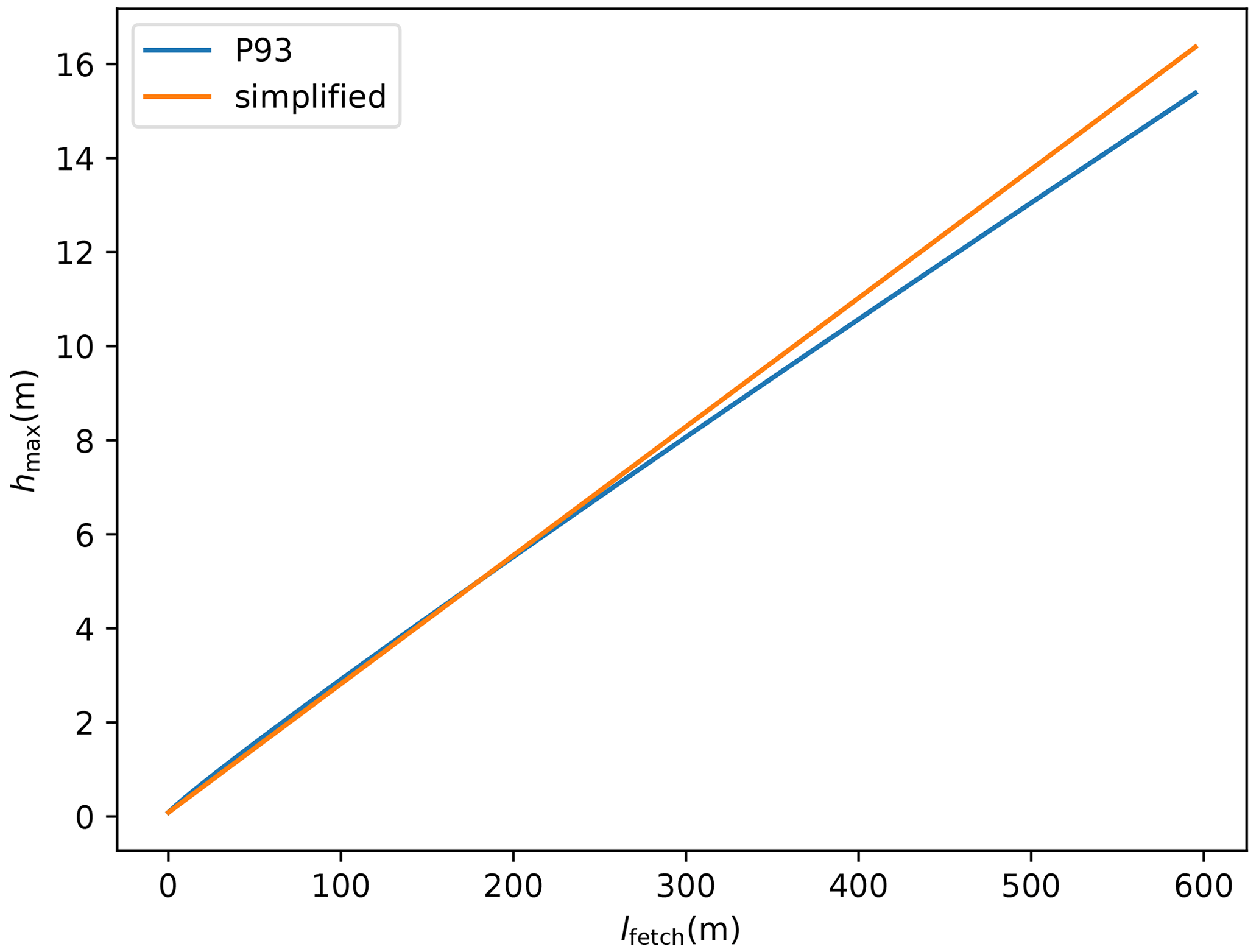
Figure A2 Comparison between the height h_max given in Sect. 3.3.2 used as an upper bound for suspension transport (blue curve) and the one computed with Eq. (10) from Pomeroy et al. (1993) (orange curve). Both heights are plotted as a function of the fetch distance as defined in Sect. 3.3.2.

Figure A3 Visualization of the maximum thread execution time spent in the different parts of SnowPappus (named as in Fig. 4) and spent in the other snow routines. This time is mainly dedicated to running the Crocus snow model.

Figure A4 Visualization of the proportion of time spent in the SnowPappus routine among all snow-related routines (“full snow routine” in Fig. 4) in terms of computing time.

Appendix B: Maximum height of the suspension layer

Following Pomeroy et al. (1993), we assume the maximum height reached by particles in the suspension layer is limited by the time available to diffuse t_d so that $h_{max}=k{u}_{*}{t}_{\mathrm{d}}$. Consequently, suspension transport grows with fetch distance. In SnowPappus, we additionally assume this is valid no matter the fetch distance. We also simplified the expression used by Pomeroy et al. (1993) to get an analytical expression, obtaining $h_{max}=h_{\mathrm{salt}}+\frac{k^{\mathrm{2}}}{\sqrt{\ln \left(\frac{h_{\mathrm{salt}}}{z\mathrm{0}}\right)\ln \left(\frac{\mathrm{5}m}{z_{\mathrm{0}}}\right)}}$. Appendix Fig. A2 compares the exact and approximated formula and shows that their difference is small. This approach assumes an abrupt end of the suspension layer at the height h_max, which is not realistic. However, it influences the model outputs only if a significant flux occurs above h_max. We can show that it happens only when wind speed exceeds 30–40 m s⁻¹ (γ becomes lower than 1, making the flux profile not integrable) or if h_max is less than ≈ 30 cm when l_fetch<10–20 m.

Appendix C: Expression of F(T)

F(T) used in Eq. (18) is expressed as follows (Essery et al., 1999):

$$\begin{array}{}\text{(C1)}& {\displaystyle }F\left(T\right){\displaystyle }={\displaystyle \frac{L_{\mathrm{s}}}{{\mathit{\lambda }}_{T}T}}\left({\displaystyle \frac{L_{\mathrm{s}}M}{RT}}-\mathrm{1}\right)+{\displaystyle \frac{\mathrm{1}}{D{\mathit{\rho }}_{\mathrm{s}}}},\end{array}$$

with T the air temperature (K), L_s the latent heat of ice sublimation, M the molar mass of water (kg mol⁻¹), R the universal gas constant (J K⁻¹ mol⁻¹) and ρ_s the water vapour saturation density (kg m⁻³).

Appendix D: Conversion formula between old and new Crocus microstructure formalism

In the current version of SURFEX, the microstructure of Crocus is described with two prognostic variables: the optical diameter D_opt and the sphericity s. In this article, we often refer to the dendricity d and grain size g_s which were used in older versions of Crocus (Vionnet et al., 2012). Carmagnola et al. (2014) proposed formulas linking D_opt, s, g_s and d. However, some errors were detected in this work, leading us to use another formula to get grain size from D_opt and s. This formula is presented here:

$$\begin{array}{}\text{(D1)}& {\displaystyle }{g}_{\mathrm{s}}{\displaystyle }=\mathrm{2}{\displaystyle \frac{D_{\mathrm{opt}}-\mathrm{2}\mathit{\alpha }(\mathrm{1}-s)}{\mathrm{1}+s}}.\end{array}$$

The formula from Carmagnola et al. (2014) is used to compute the dendricity d from s and D_opt.

Appendix E: Properties of deposited snow in the case of simultaneous snowfall and wind-driven redeposition

We consider here the case when during a time step, a mass m_SP and m_BS (kg m⁻²) of snow respectively coming from solid precipitation and wind-driven redeposition has to be added to the snowpack during a simulation time step. Optical diameter D_BS and sphericity s_BS of the deposited windblown snow are given in Sect. 3.6. Solid precipitation sphericity s_SP and optical diameter D_SP are computed as in the default Crocus configuration, described in Vionnet et al. (2012). In this case, a layer of total mass $m=m_{\mathrm{SP}}+m_{\mathrm{BS}}$ is added to the snowpack. Its properties s and D are given by the weighted average of blowing-snow and solid precipitation properties.

$$\begin{array}{}\text{(E1)}& {\displaystyle }s& {\displaystyle }={\displaystyle \frac{m_{\mathrm{SP}}{s}_{\mathrm{SP}}+m_{\mathrm{BS}}{s}_{\mathrm{BS}}}{m_{\mathrm{SP}}+m_{\mathrm{BS}}}}\text{(E2)}& {\displaystyle }D& {\displaystyle }={\displaystyle \frac{m_{\mathrm{SP}}{D}_{\mathrm{SP}}+m_{\mathrm{BS}}{D}_{\mathrm{BS}}}{m_{\mathrm{SP}}+m_{\mathrm{BS}}}}\end{array}$$

Appendix F: Masks applied to 2D simulations and observations

The forests, glaciers, lakes and rivers, and cities in the study zone are masked in our simulations and observation datasets. For the forest mask, the BD FORET^® V2 dataset has been used (IGN©, 2021a) with a masking threshold of 25 % of forested sub-pixel area. Lakes and rivers are masked following data from BD TOPO^® (IGN©, 2021b) and glaciers following the Randolf glacier inventory. A pixel is masked when more than 50 % of the surface of a pixel is covered. In the valley, the urban areas around the cities of Bourg d'Oisans, Allemont and Saint Michel de Maurienne are also masked.

Appendix G: Numerical performance

In this section, we describe the numerical performance of the SnowPappus model to discuss its suitability for the goal of applicability in large-scale systems operated at hectometre resolution.

Computation time was measured for 1 complete simulation year on the simulation domain covering the Grandes Rousses range (Sect. 4.1). Computations are done using one node of the current Météo-France supercomputer made of two AMD Rome 2.2 Ghz CPUs, giving a total 128 computing cores and 256 Gb of node RAM. For the Grandes Rousses domain, the maximum possible number of threads is 101 (see Sect. 3.6) To time the execution of different parts of the code on a distributed set of cores, we use the DrHook profiling tool (Saarinen et al., 2005). To obtain the user run time of non-overlapping and blocking code sections, we sum the maximum computing thread time for each code section.

Figure A3 shows the maximum thread execution time for each code section of the SnowPappus blowing-snow model and compares these durations to the full snow routine of SURFEX, which contains mainly the SnowPappus routine and the Crocus snow model, for different degrees of parallelization. Its execution time decreases sharply with the number of threads used but reaches a plateau at 60 cores and above. Almost all of the SnowPappus computing time is dedicated to MPI communications. Therefore, the proportion of time spent in the SnowPappus routine grows with the number of threads used, eventually becoming more time-consuming than Crocus (it is shown more visually in Appendix Fig. A4), indicating it benefits less than Crocus from increased parallelization. It can be explained by the increased number of MPI blocking communications. Indeed, communication time and waiting time between threads should grow with the number of subdomains as the workload cannot be equally shared among them.