the Creative Commons Attribution 4.0 License.
the Creative Commons Attribution 4.0 License.
 | 09 Jan 2024
The wave-age-dependent stress parameterisation (WASP) for momentum and heat turbulent fluxes at sea in SURFEX v8.1
Marie-Noëlle Bouin
Cindy Lebeaupin Brossier
Sylvie Malardel
Aurore Voldoire
César Sauvage
A widely applicable parameterisation of turbulent heat and momentum fluxes at sea has been developed for the SURFEX v8.1 surface model. This wave-age-dependent stress parameterisation (WASP) combines a close fit to available in situ observations at sea up to wind speed of 60 m s−1 with the possibility of activating the impact of wave growth on the wind stress. It aims in particular at representing the effect of surface processes that depend on the surface wind according to the state of the art. It can be used with the different atmospheric models coupled with the surface model SURFEX, including the CNRM-CM climate model, the operational (numerical weather prediction) systems in use at Météo-France, and the research model Meso-NH. Designed to be used in coupled or forced mode with a wave model, it can also be used in an atmosphere-only configuration. It has been validated and tested in several case studies covering different surface conditions known to be sensitive to the representation of surface turbulent fluxes: (i) the impact of a sea surface temperature (SST) front on low-level flow by weak wind, (ii) the simulation of a Mediterranean heavy precipitating event where waves are known to influence the low-level wind and displace precipitation, (iii) several tropical cyclones, and (iv) a climate run over 35 years. It shows skills comparable to or better than the different parameterisations in use in SURFEX v8.1 so far.
- Article
(12227 KB) - Full-text XML
- BibTeX
- EndNote


1.1 Background
Turbulent air–sea interactions are known to play a central role in modulating heat and moisture exchanges at interannual to climatic scales. They also control the major part of the heat, moisture, and momentum exchanges in tropical cyclones (TCs) and, as a consequence, have a strong impact on cyclone intensity (e.g. Emanuel, 2004; Bryan, 2012). Their accurate representation in climate or numerical weather prediction (NWP) models is thus a key step towards better modelling the climate evolution and extreme weather events.
Because the turbulent fluctuations in surface parameters cannot be represented explicitly in atmospheric models, turbulent fluxes are computed using “bulk” parameterisations as functions of mean atmospheric variables at the surface within the framework of the similarity theory proposed by Monin and Obukhov (1954, MOST). For the wind stress τ, it reads as follows:
with ρ the air density, u* the friction velocity, ΔU the difference between the wind speed at a reference level and the surface current Uc, and Cd the drag coefficient. Note that bulk algorithms generally include the effect of gustiness in the turbulent fluxes by including a term Ug in the ΔU difference, such that ΔU reads , with Ux, Uy the components of the surface wind and Ucx, Ucy the components of the surface current. This gustiness term is not explicitly mentioned in the present work but is taken into account in the SURFEX v8.1 version of all bulk algorithms used here. Similarly, the heat fluxes are expressed as follows:
with cp the air heat capacity and Lv the latent heat of vaporisation. Δθ and Δq represent the vertical air–sea gradients of potential temperature and specific humidity, respectively. In neutral conditions and in the surface layer, where u* is supposed to be constant with height, U(z) may be represented as a logarithmic profile:
where κ is the von Karman's constant (≈0.4) and z0 the roughness length. Equivalently, one can write
in neutral conditions and in the absence of a surface current.
The roughness length z0 is expressed as the sum of two terms representing the behaviour of the surface in (respectively) rough and viscous regimes (Charnock, 1955; Beljaars, 1994):
with ν the kinematic viscosity of dry air, g the gravitational acceleration, and α the Charnock coefficient. The Charnock coefficient was originally assumed to be constant, but its dependence on wave parameters allows the drag coefficient to vary more explicitly with the sea state. Defining the transfer coefficients Cd, Ch, and Ce with reasonable accuracy in various conditions of surface wind, stability, and sea state has been the subject of a considerable amount of work by many expert teams for at least the last 50 years and the motivation for many dedicated field campaigns.
1.2 Constraints from observations
Direct observations of the turbulent fluxes at sea on buoys, ships and platforms provide constraints on the mean value of the neutral drag coefficient and its growth with wind speed in the range of 10 m wind speed between 5 and 20 m s−1 (e.g. Edson et al., 2013). In this wind range, the momentum transferred from the wind to the sea surface is mainly used for the waves to grow up to a well-developed sea, in equilibrium with the wind (e.g. Janssen, 1989, 2004). The part of the wind stress absorbed by the waves has been formulated to be dependent on the stage of development of the wind sea or wave age (defined as the ratio of the wave phase speed for the peak of the wave spectrum to the near-surface wind) by Snyder et al. (1981) and Komen et al. (1984). The wave development, in turn, impacts the Charnock parameter and roughness length through Eq. (5) and the friction velocity through Eq. (4). Observations carried out with extreme care and in mainstream conditions (i.e. in the absence of swell or strong surface currents) do indeed show a large variability in the friction velocity and in the drag coefficient at a given wind speed (Fig. 1). Several studies based on theoretical considerations (Kitaigorodskii, 1965; Janssen, 1989) or field observations (Smith et al., 1992; Donelan et al., 1993) attribute part of this variability to the effect of the wave growth on z0. Wave steepness (wave height divided by wavelength) is also a good proxy for the sea-state impact on the surface roughness (Taylor and Yelland, 2001). Several parameterisations of the wind stress with dependence on the wave age have been developed to be used in wind–wave coupled models (e.g. Oost et al., 2002; Drennan et al., 2003; Janssen, 2004). As a pioneer in the wind–wave coupling domain, the European Centre for Medium-Range Weather Forecasts (ECMWF) used coupled models for operational forecasts since 1998 and obtained improvement for surface pressure in medium-range NWP and for the 500 hPa geopotential at seasonal scales (Janssen et al., 2001).
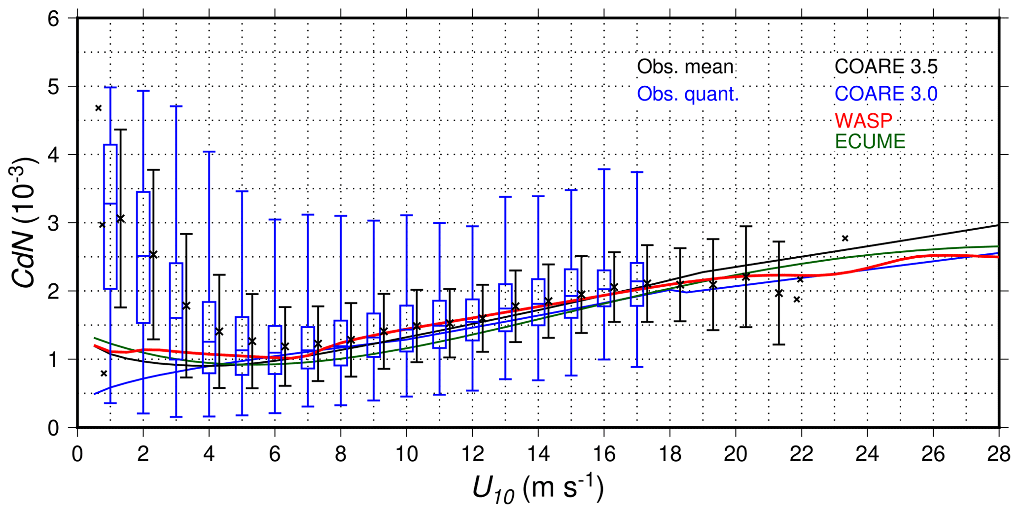
Figure 1Neutral drag coefficient with respect to 10 m wind speed for different parameterisations (COARE3.5, Edson et al., 2013; COARE3.0, Fairall et al., 2003; ECUME, Roehrig et al., 2020; and WASP) and in situ eddy covariance observations (see text and Appendix B for details). The black symbols and error bars indicate the mean values and standard deviation for observations in each 1 m s−1 bin (with five values or more) and the blue boxes and whiskers indicate the median and 10 %, 25 %, 75 %, and 90 % quantiles (with 10 values or more).
For wind speed above 30 m s−1, the coupling regime controlling the stress transfer from the atmosphere to the waves is thought to be less dependent on the wave growth, as most waves are breaking. Direct measurements of wind stress are sparse but show no clear dependence on the wave age but a saturation or decrease for wind speeds above 30 to 35 m s−1 (Powell et al., 2003). This saturation itself is confirmed by other (more or less direct) observations (e.g. Black et al., 2007; French et al., 2007; Jarosz et al., 2007; Vickery et al., 2009; Bell et al., 2012), but the exact corresponding 10 m wind speed where it occurs, the maximum value of the drag coefficient, and its behaviour at higher wind speeds are still very uncertain. Indeed, all available estimates beyond 30 m s−1 are highly scattered (see Figs. 2 and B2). Based on observations, there is no evidence that the scattering of the drag coefficient in wind speeds higher than 30 m s−1 may be due to wave age. According to previous work, the physical mechanisms likely to explain the observed saturation or decrease in the drag coefficient above 30 m s−1 are airflow separation due to wave breaking (Kudryavtsev et al., 2014), changes in the wind profile close to the surface due to a high concentration of sea spray (Andreas, 2004), or the inclusion of non-linear effects in the critical layer theory for wave growth (Miles, 1957) with an explicit calculation of the momentum transferred to capillary–gravity waves (Janssen and Bidlot, 2023). The saturation or decrease observed for cyclonic wind speeds must be reproduced in a parameterisation (using an analytical function or capping) to match the observations and enable a more realistic simulation of the tropical cyclone intensity (Majumdar et al., 2023).
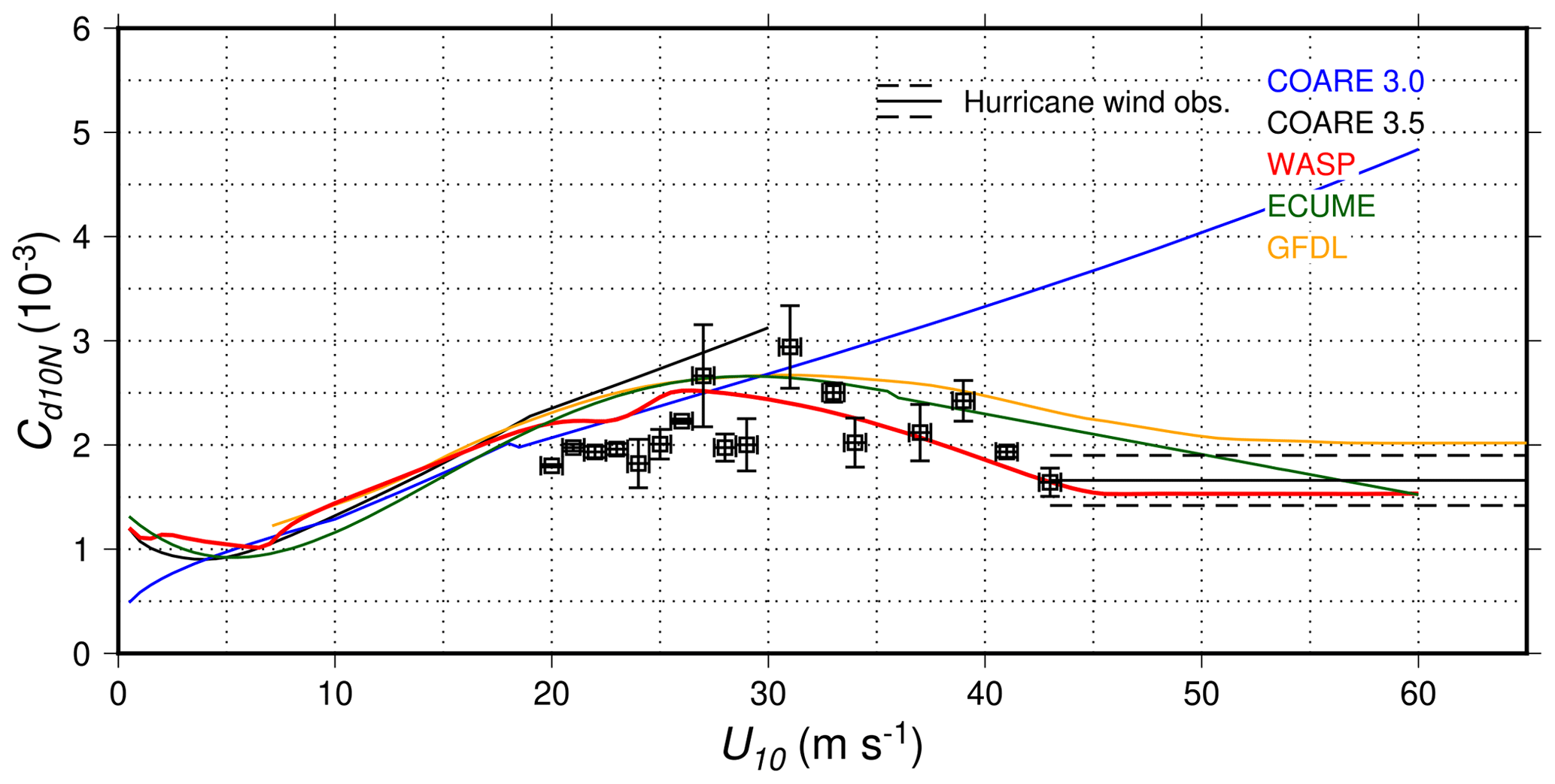
Figure 2Neutral drag coefficient with respect to 10 m wind speed for different parameterisations (COARE3.0, Fairall et al., 2003; COARE3.5, Edson et al., 2013; WASP; ECUME, Roehrig et al., 2020; and GFDL, Chen et al., 2020) and summary of observations up to 60 m s−1.
Observations of the heat transfer coefficients show no clear dependence on the wind speed nor on the sea state. Estimations of sensible heat flux at sea from sonic anemometers are extremely noisy, resulting in a large dispersion between datasets (Figs. 3 and B1). Measurements of the latent heat flux are done by gas analysers, which are very sensitive to rain, high humidity rates at sea, sea spray, and pollutants. All of this results in highly scattered values, even in the 5–20 m s−1 wind speed range (Fig. B1). However, surface heat transfer plays a central role in TC intensification (e.g. Emanuel, 2018) and correctly representing it for strong winds in NWP models is a key step towards a better forecast of TC intensity. Besides, heat transfer plays a central role in modulating the climate-scale dynamics (in particular in the intertropical band) and can also control local processes even at low winds (e.g. Redelsperger et al., 2019).
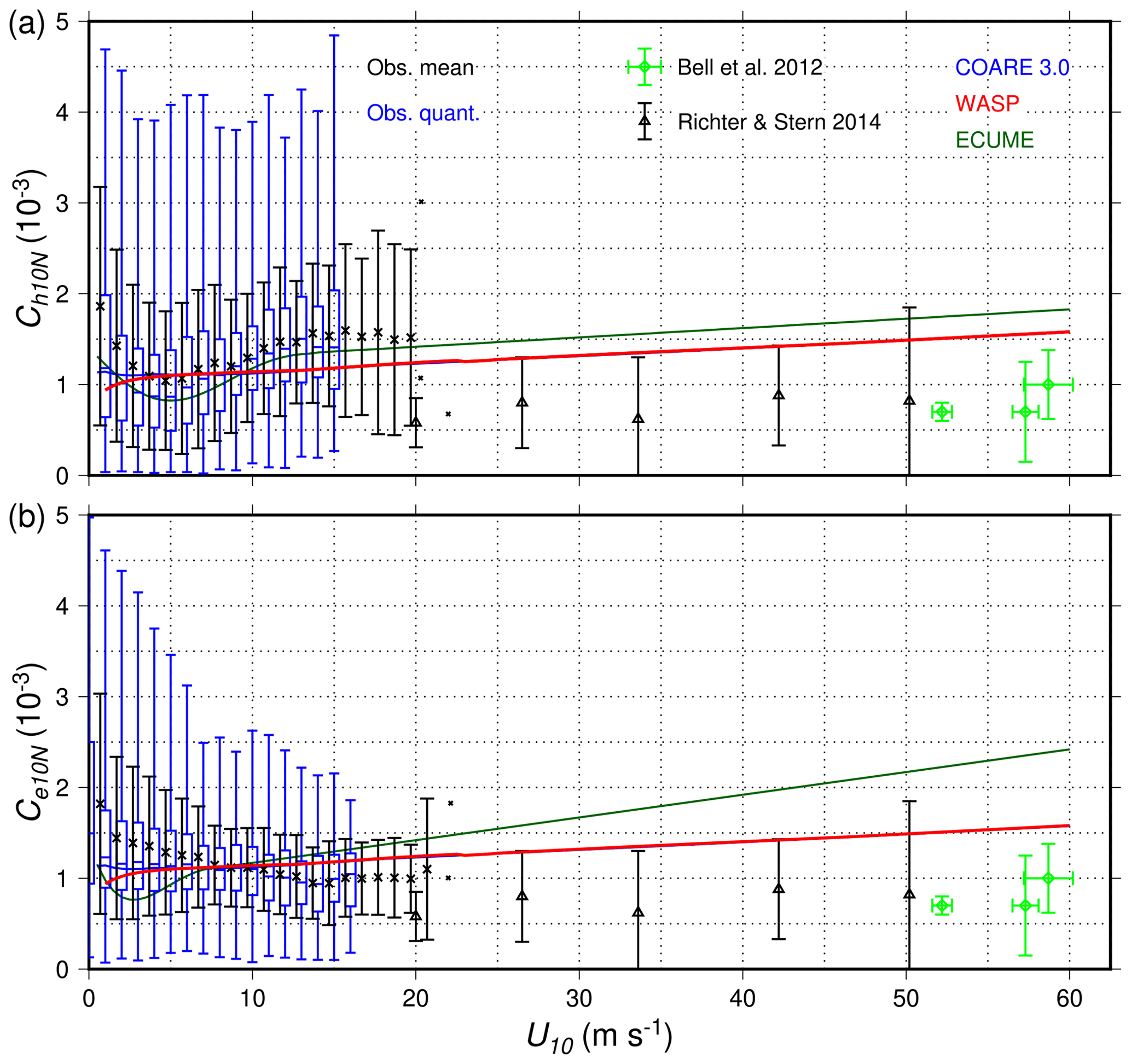
Figure 3Neutral coefficient for sensible (a) and latent (b) heat fluxes at 10 m with respect to 10 m wind speed for different parameterisations (COARE3.0 (Fairall et al., 2003), blue line; WASP, red line; and ECUME (Roehrig et al., 2020), dark green line) and in situ eddy covariance observations and estimates of up to 60 m s−1 (see text). Note that WASP and COARE3.0 are almost superimposed. Black and blue symbols as in Fig. 1.
1.3 Rationale for this work
Several parameterisations of sea surface turbulent fluxes are available in the current SURFEX v8.1 surface model (Masson et al., 2013), the surface scheme embedded in the atmospheric models used at Météo-France. None of them, however, provides a match to observations for all wind speeds, including the cyclonic conditions, and the possibility of accounting for the wave growth effect on the roughness length and drag coefficient. The ECUME parameterisation (Roehrig et al., 2020, updated from its initial version in Belamari, 2005) is the default scheme used for operational NWP in the non-hydrostatic, limited-area model AROME (Seity et al., 2011) and in the global model ARPEGE (Courtier et al., 1991). ECUME is also used in ARPEGE within the CNRM-CM configurations for climate simulations (Déqué et al., 1994). It is also commonly used for case studies with the research-oriented, non-hydrostatic, Meso-NH model (Lac et al., 2018). ECUME has been built by fitting scale parameters for wind, temperature, and humidity on observations and enables a close match of the transfer coefficients to observations (Figs. 1 and B2). These transfer coefficients are expressed as polynomial functions of the 10 m wind speed only (the roughness length is a diagnostic parameter; Eqs. (4) and (5) are not part of the bulk algorithm). The COARE 3.0 parameterisation (Fairall et al., 2003) can also be used in SURFEX v8.1. It enables representing the impact of sea state on the roughness length through the use of the parameterisations of Oost et al. (2002) or Taylor and Yelland (2001) (our Fig. 4b and c). It can also be used in coupled mode with a wave model, the Charnock coefficient (Eq. 5) being computed within the wave model. Using SURFEX with the wave model WAVEWATCH III™ (WW3, Tolman, 2009) has been made possible by the implementation of a surface coupling interface with the OASIS coupler in SURFEX by Voldoire et al. (2017). COARE 3.0 has been fitted to observations of wind stress and heat fluxes in the tropics, for wind speeds up to 18 m s−1. It provides a good match with observations of wind stress up to 20 m s−1 (Fig. 1) but does not reproduce the decrease in the drag coefficient for winds higher than 30 m s−1 (Figs. 4a and 2). As a consequence, it is not suitable for representing the development of TCs or strong storms.
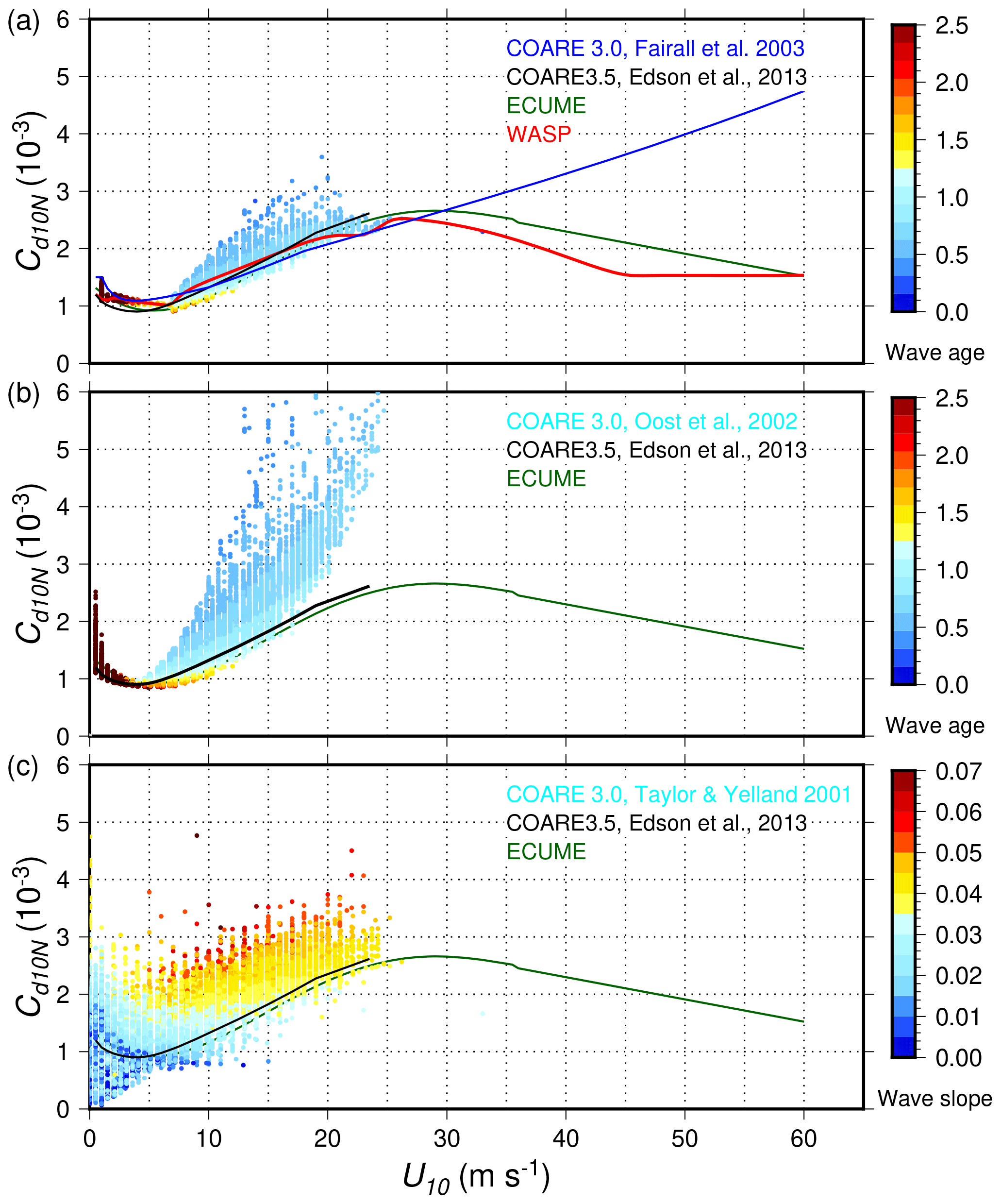
Figure 4Neutral drag coefficient with respect to 10 m wind speed for the parameterisations implemented in SURFEX v8.1 (a) (COARE 3.0, Fairall et al., 2003; COARE3.5, Edson et al., 2013; ECUME, Roehrig et al., 2020; and WASP, present study), COARE 3.0 with dependence on the wage age (b – colour scale, Oost et al., 2002), and COARE 3.0 with dependence on the wave steepness (c – colour scale, Taylor and Yelland, 2001). The surface data used to compute the drag coefficient with wave impact in (a), (b), and (c) are the hourly observations of the LION moored Météo-France buoy (centre of the Gulf of Lion) between 2001 and 2014.
The new parameterisation presented here combines the two aspects of wind–wave coupling and reproducing the decrease in the drag by cyclonic winds. It is based on a very large set of field observations (see Sect. 2.1 for their selection) and ensures that their mean behaviour, in terms of drag and heat transfer coefficients, is well reproduced for wind speeds up to 60 m s−1. It is also based on the Charnock relationship with a dependency of the Charnock parameter on the wave age for wind speeds between 7 and 22 m s−1, corresponding to the growth of wind sea (Janssen, 2004):
where is the wave age and A and B are polynomial functions of U10 (see Appendix A1 for more details). Note that, according to Janssen (2004), the wave age should be computed as rather than , but we use Eq. (6) for computing-cost reasons and we checked that the differences are negligible. For wind speeds of less than 22 m s−1, the WASP transfer coefficients closely follow those derived by Edson et al. (2013), using a very large and carefully screened dataset. We do not pretend here to improve much the state of the art of turbulent fluxes at sea that can be used for wind–wave coupling but rather to design a tool that can be used with every atmospheric model coupled with SURFEX v8.1, producing realistic wind stress and heat fluxes at every wind speed. In addition, the drag coefficient varies as a function of the wave age for a given wind speed in the moderate- to strong-wind range where wave growth is the major process absorbing the wind energy. The next section presents the principle used for building the new parameterisation, the observations used to check the mean values of the transfer coefficients for a given wind speed, and the dependency of the drag coefficient on wage age. These options are discussed with respect to the literature and information from various datasets. Section 3 presents the four case studies that were used to validate and test this parameterisation. Some conclusions are given in Sect. 4.
We present here, first the observations that we retained to fit the mean values of the transfer coefficients and then the transfer coefficients we obtained as functions of the 10 m wind speed. Unless specified otherwise, the transfer coefficients developed in this work correspond to neutral transfer coefficients at the height of 10 m. They can be expressed as follows:
with x=d for wind stress, h for sensible heat, and e for latent heat and where z0x is a roughness length characterising the surface properties for the given variable. The non-neutral transfer coefficients used in Eqs. (1) and (2) are expressed for a given height z as follows:
with representing the stability parameter and L the Obukhov length. Neutral conditions correspond to ψ=0, and the Obukhov length is a function of the scaling parameters and values of the wind, temperature, and humidity. The stability functions ψ are defined as in Beljaars and Holtslag (1991) with the modifications of Fairall et al. (2003) concerning the free-convection conditions (see Appendix A2 for their full definition). WASP is intended to be used either in a coupled mode through the SURFEX v8.1–OASIS3-MCT coupling interface (Voldoire et al., 2017) or in a forced mode using outputs of a wave model. The wave age in Eq. (6) is computed using the wave phase speed for the peak of the wind sea and not of the total wave field, and the parameters sent by WW3 to OASIS (starting with WW3 v5.14) have been changed to include this phase speed. But using WASP without wave information is also possible. For the latter use, transfer coefficients are functions of the wind speed corresponding to the mean value taken in coupled mode with a well-developed wind sea (“mean values” hereafter), to ensure that the coupled-mode variability actually corresponds to the wave effect. Section 2.1 presents the datasets used to derive these mean values (as explained in Sect. 2.2.1) and the variation in the surface roughness with sea state is presented in Sect. 2.2.2.
2.1 Selection of observations
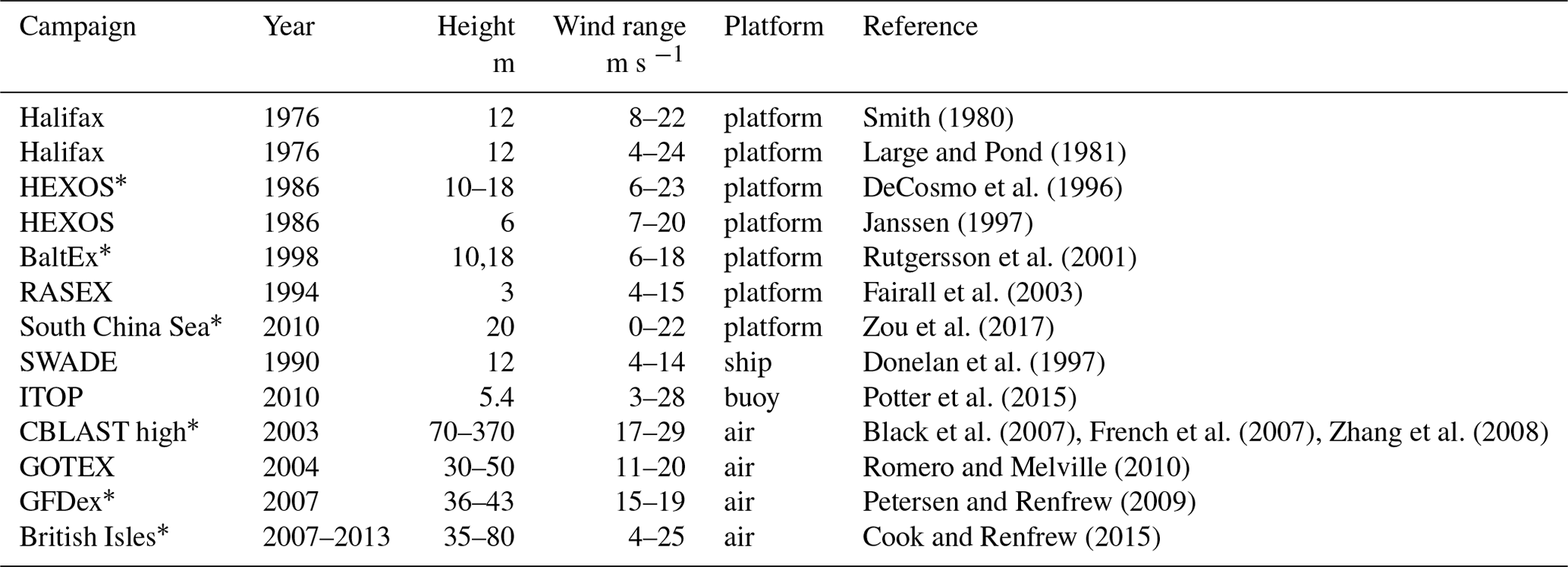
The parameterisation presented here is meant to be used for atmospheric numerical modelling, either operationally with the models of Météo-France of for a large variety of case studies with Meso-NH, with typically the first level at 5 to 20 m above sea level (a.s.l.). Whereas it may be tempting to use much finer sampling close to the surface to better represent its influence on the surface-layer or boundary-layer processes, we believe that doing so within the MOST framework leads to inconsistency (see Pelletier et al., 2021, for a discussion). The mean values of the transfer coefficients should be representative of a large number of neutral conditions, and the only variability introduced is the impact of the wave age for wind speeds between 7 and 23 m s−1 (see Sect. 2.2.2). Turbulent fluxes and transfer coefficients are usually derived from in situ measurements recorded using high-frequency sensors (sonic anemometers and gas analysers) with either the eddy covariance (EC) or the inertial–dissipative (ID) methods. While obtaining reliable estimates using the ID method is easier and more straightforward, it implies strong assumptions on the surface-layer structure, which restrict its use. In this study and for wind conditions up to 25 m s−1, we use only carefully checked datasets from measurements at 5 m a.s.l. or above computed using the EC method. Thanks to the effort of the observing community, a large number of such datasets exist and many of them were already used by Edson et al. (2013) for deriving the wind stress parameterisation COARE 3.5 (see Table B1 for a list). This results in more than 27 000 individual data (representing 10 to 30 min of measurements each) for Cd, 21 000 for Ch and 24 000 for Ce. This covers the wind speed up to 22 m s−1 for Cd, and 20 m s−1 for Ch and Ce. These observations were binned in intervals of 1 m s−1 of wind speed, screened and quality checked. The screening consists of evaluating the symmetry of the binned distributions and whether they correspond rather to normal or log-normal laws. Depending on the results, outliers more than 4 standard deviations from the mean values were removed.
Other historical datasets available in the literature (see Table B2) have been used for the range of wind speed up to 30 m s−1. Direct EC measurements in strong winds are scarce and usually made airborne at height between 30 and 500 m a.s.l. (Black et al., 2007; Vickery et al., 2009; Cook and Renfrew, 2015). For extreme winds between 30 and 60 m s−1, only very few observations are available, especially for the heat transfer coefficients. Some of them are derived from profiles of dropsondes (Powell and Ginis, 2006), mostly computed indirectly from the effect of the wind stress on the oceanic surface layer, which is more easily sampled than the atmospheric boundary layer in extreme conditions (Jarosz et al., 2007; Hsu et al., 2017; Richter and Stern, 2014). The observations used in this study that correspond to extreme conditions are listed in Table B3. Among them, some are derived from the oceanic response to tropical cyclones using inversion techniques and come with uncertainties higher than more direct estimates (dropsondes). All these data were used as constraints to derive the transfer coefficients, with different principles for the drag or the heat transfer coefficients, as detailed below.
2.2 Drag coefficient
The neutral drag coefficient is first constructed as a mean value, depending on the wind speed only, and fitted to available observations in the wind range from 5 to 60 m s−1. Then, a variability depending on the wave age in the wind range of 7 to 25 m s−1 is added to the mean value.
2.2.1 Mean fit to observations
In the wind range covered by the in situ, EC observations used to derive the COARE 3.5 parameterisation (Edson et al., 2013), namely 0 to 21 m s−1, the mean value of the neutral drag coefficient is aligned on the COARE 3.5 parameterisation, which we regard as the state of the art for drag coefficient. For wind range above 21 m s−1, we use data published in the literature (Tables B3 and B2) from less direct measurements, like airborne observations transformed into 10 m wind speed, and measurements on platforms, which may be flawed by the flow distortion. These observations are shown in binned form of 1 m s−1 wind speed in Figs. 1 and 2 (see also Fig. B2 for the detail of observations above 30 m s−1). Between 25 and 45 m s−1, a polynomial function of the wind speed is used to represent the drag coefficient. This function is fitted on the data with weighting based on the uncertainties published with the data (average values and standard deviation are computed with weights equal to the inverse of the variance of the individual datasets). The root mean square of the residuals on Cd is 3.35 ± 0.32 × 10⁻⁴. For the wind speed range above 45 m s−1, we consider a constant drag coefficient in the continuity of the previous wind speed range, with a value 1.56 × 10⁻³. The weighted average of the published datasets for the drag coefficient in this wind range is 1.66 ± 0.24 × 10⁻³, compatible with the value chosen for this constant part of the drag coefficient.
2.2.2 Variability with wave growth
We aim here at introducing some variability in the drag coefficient with respect to the wave growth. In their seminal work, Janssen (1989, 1991, 2004) integrated the input term Sin in the wave model to derive the part of the wind stress absorbed by the wave growth and to scale the Charnock coefficient. This approach, used for two-way coupling in the operational Integrated Forecasting System (IFS) at ECMWF (Janssen, 2004), is well adapted to operational use with fixed resolutions, and careful tuning and upgrades of the wave and atmospheric model physical parameterisations. Conversely, it is not appropriate for being included in SURFEX v8.1, which is intended to be used with several atmospheric models at various resolutions, for NWP, climate, or research applications with variable configurations. Indeed, the Charnock parameter computed this way is mainly sensitive to the high-frequency tail of the spectrum (see Eq. 5.22 and 5.24 in Janssen, 2004), which is always parameterised in wave models, because high frequencies cannot be represented explicitly. Some sensitivity tests showed that there is little variability in the Charnock parameter due to the wave field variability for a given wind speed. An alternative representation of the capillary–gravity waves and of the part of momentum they absorb is nevertheless provided by Janssen and Bidlot (2023) and should be tested. In present configurations, the benefit of coupling with a wave model are reduced. The WASP approach used here has two advantages, compared to the Charnock parameter approach: (i) it is based on the phase speed or peak period of the waves, which is one of the most accurate parameters produced by wave models, and easy to compare to observations, unlike the Charnock parameter against observations; (ii) the Charnock parameter is defined here differently depending on the range of wind speed considered, enabling us to add variability due to wave age for wind speeds going from moderate to strong only. In the wind speed range between 7 and 25 m s−1 where the roughness dependency on the wind sea is maximal, the Charnock parameter is expressed as in Eq. (6). Below 7 m s−1, the Charnock coefficient is a power function of U10 and a polynomial of U10 above 25 m s−1. The WASP drag coefficient, with a dependence on the wave age, is shown in Fig. 4a.
2.3 Heat fluxes
The principle retained here for building the heat flux transfer coefficient is very similar to the one of the COARE 3.0 (Fairall et al., 2003) parameterisation. It is clear from Eq. (7) that the neutral transfer coefficients both for sensible and latent heat fluxes depend only on the roughness lengths z0x and z0. The values of the neutral transfer coefficients for turbulent heat ChN and CeN correspond to those of the COARE 3.0 parameterisation. Then, Eq. (7) is inverted to obtain the value of z0x, z0 being obtained in WASP as explained in Sect. 2.2. In the following, we use datasets of available observations to evaluate these parameters for wind speed in the range 0 to 60 m s−1. These observations are grouped in direct, EC measurements between 0 and 21 m s−1 for ChN and 0 and 19 m s−1 for CeN and less direct measurements for higher wind speed, available as mean values with estimates of uncertainties for a given wind range or in binned form (see Fig. 3).
2.3.1 Sensible heat flux
The direct EC observations have a mean value of 1.388 ± 0.044 × 10⁻³ for ChN and the high wind or less direct observations (in the range 11–60 m s−1) a weighted mean of 1.081 ± 0.020 × 10⁻³. The mean values are computed as weighted means using the standard deviations of different groups of observations as weights. All together, the whole dataset gives a weighted mean of 1.143 ± 0.021 × 10⁻³, very close to the constant value of ChN in WASP. The mean difference and standard deviation between WASP and the binned values of this dataset are 2.1 × 10⁻⁴ ± 3.5 × 10⁻⁵.
2.3.2 Latent heat flux
The direct EC observations have a weighted mean of 1.159 ± 0.034 × 10⁻³ for CeN and the high wind or less direct observations (in the range 11–60 m s−1) a weighted mean of 1.155 ± 0.012 × 10⁻³. All together, the whole dataset gives a weighted mean of 1.156 ± 0.011 × 10⁻³, even closer to the constant value of CeN in WASP than for ChN. The mean difference and standard deviation between WASP and the binned values of this dataset are 1.3 × 10⁻⁴ ± 3.4 × 10⁻⁵.
2.4 Direct comparison
An offline test was performed to assess the differences between the current version of ECUME used in the Météo-France NWP and climate runs on the one hand and WASP on the other. The SURFEX v8.1 model was used to compute the friction velocity and turbulent heat fluxes with either the ECUME or WASP scheme on the same dataset corresponding to observed atmospheric parameters, SST, and wave parameters Hs and Tp. This dataset consists of more than 53 000 hourly in situ measurements at the Lion buoy, located in the Gulf of Lion, between December 2001 and February 2014. They represent a large range of atmospheric conditions (Fig. 5) with wind up to 25 m s−1, air temperature between 5 and 28 ∘C, relative humidity down to 40 %, and wave age () as low as 0.4 due to strong wind and short fetch in mistral conditions. Strong winds in the Gulf of Lion correspond overall to the mistral and tramontane winds blowing offshore, resulting in strongly unstable conditions with dry air, young waves, and significant wave height up to 6 m. Figure 6 shows the difference obtained using WASP rather than ECUME on the fluxes of momentum and sensible and latent heat, as a function of the different surface conditions at the buoy. Warm colours indicate positive differences (the fluxes obtained using WASP are higher than those obtained using ECUME) and blue shades indicate negative differences. The comparison of friction velocities obtained using WASP and ECUME (Fig. 6a) shows that the difference does not depend at first order on the wind speed but on the wave age. As expected, young waves give higher friction velocities than older waves. The larger scattering of the difference which is obtained for the lowest and highest wave ages is an artefact due to the smaller size of the sample. For more common conditions, i.e. between 7 and 20 m s−1 and wave ages below 1, WASP gives consistently higher friction velocities than ECUME (8 %). In weaker wind conditions, the difference is not significant.
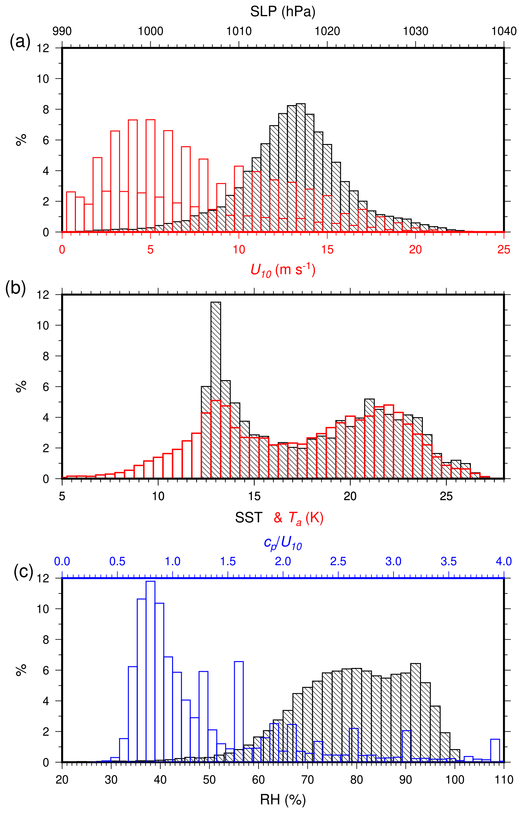
Figure 5Probability distributions of the data recorded at the Lion buoy: U10 (red) and sea level pressure (black, a), SST (black) and air temperature (red, b), and relative humidity (black) and wave age (, blue, c). These data are used to force the ECUME and WASP schemes for a direct intercomparison.
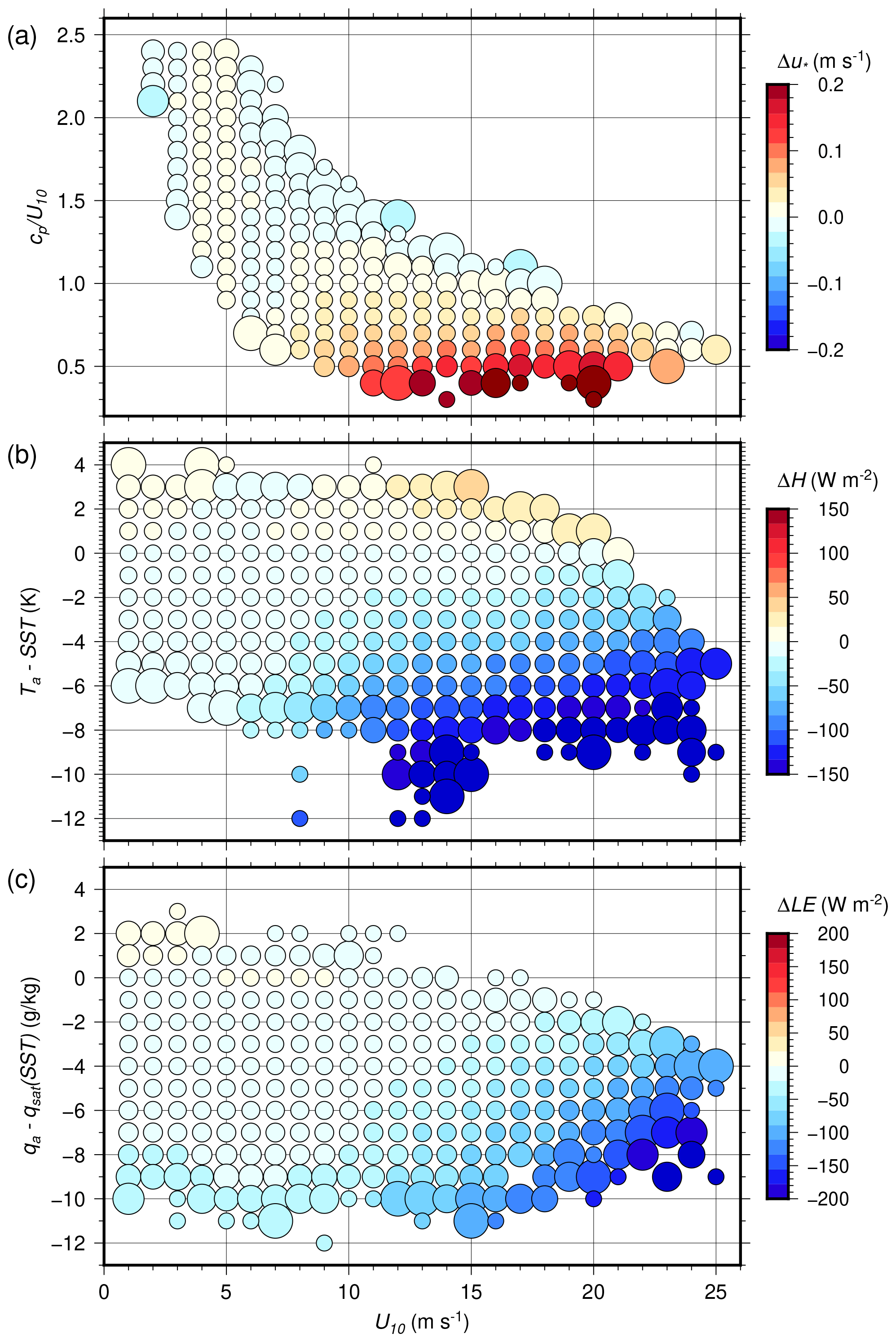
Figure 6Differences between WASP and ECUME (coloured dots) for the friction velocity (a) and the sensible (b) and the latent (c) heat fluxes. The differences are mapped as a function of the 10 m wind speed on the x axis and of the wave age (a), the air–sea temperature difference (b), and specific humidity difference (c) on the y axis. The size of the symbols indicates the standard deviation of the difference.
Both sensible and latent heat fluxes are generally lower with WASP than with ECUME (Fig. 6b, c). The difference in sensible heat flux is very dependent on the air–sea temperature gradient, especially for winds above 10 m s−1. In very unstable conditions, which are rather common in the Gulf of Lion, the difference reaches −150 W m−2, for only 30 to 40 W m−2 in stable conditions. The latent heat flux is lower whatever the conditions, except for weak wind and warm and moist conditions that are rarely met in the Gulf of Lion. It can be expected therefore that heat fluxes will be lower with WASP than with ECUME when simulating tropical cyclones, at least in the intensification phase with wind speed up to 25 m s−1.
A key step of building a parameterisation consists of checking its behaviour in representative conditions. To do this, we selected (i) a case study of weak wind and weak heat fluxes but where the low-level flow is influenced by the effects of a change in stratification on the non-neutral drag coefficient; (ii) a strong-wind case where coupling wind and waves is known to influence the low-level flow and the location of heavy precipitation; (iii) several representative cases of tropical cyclones where both wind stress and heat fluxes control maximum wind speed and minimum sea level pressure; and (iv) a coarse, atmosphere-only climatic run where the energetic balance over several decades depends on both the wind stress and heat fluxes in weak to moderate wind conditions. Cases (ii) to (iv) were performed using the operational models of Météo-France in configurations close to the operational ones. Case (i) was performed using the research model Meso-NH in the same configuration as in Redelsperger et al. (2019). Case (iii) was of special importance for building WASP as its results led to the tuning of the parameterisation for wind above 20 m s−1, where observations do not provide enough constraints. Among these cases, only case (ii) explicitly takes into account the wave effect using sea state modelled by WW3; other cases use WASP with the wave age computed as a function of the 10 m wind speed.
3.1 Weak wind conditions: an Iroise Sea case
The case study of a weak low-level flow across a sharp SST front in the Iroise Sea (Redelsperger et al., 2019, R2019 hereafter) is used to assess WASP in calm atmospheric conditions, with a strong change in atmospheric stratification over a few kilometres. The configuration used here is the same as in R19, and the reader can refer to this paper for a full description of the case study and modelling configuration.
3.1.1 Atmospheric conditions and modelling configuration
The Ushant SST front is a sharp surface front (3 to 5 ∘C over ∼ 20 km) of barotropic (tidal) origin, which is usually present from March/April to October in the Iroise Sea and moves of about 5 km throughout the day due to the tidal currents. On the day of the study (2 September 2011), the low-level wind was 3 m s−1 from the south-west, crossing the front from the warm to the cold side with a ∼ 45∘ angle. The 2 m temperature was close to 15 ∘C, in contrast with the 17 ∘C or higher SST on the warm side of the front and 15 ∘C or lower SST on its cold side, resulting in unstable to neutral atmospheric stratification. The Meso-NH model was used for a 12 h simulation with three two-way nested domains with a horizontal resolution as fine as 100 m on the central domain covering 45 × 50 km across the front. The surface conditions (SST) were provided hourly by a simulation using the Model for Applications at Regional Scales (MARS-3D), zoomed at 500 m (Lazure and Dumas, 2008). The atmospheric initial and boundary conditions of the largest domain were taken from the AROME-France operational analyses at 2.5 km (Seity et al., 2011). In the reference simulation, the surface turbulent fluxes were parameterised using COARE 3.0, which is suitable for the weak wind conditions. In R2019, it is shown that the impact of the SST front on the marine atmospheric boundary layer (MABL), although in agreement with published results about its effects and intensity (e.g. Small et al., 2008), differs by the mechanism involved. The sharpness of the front combined with the weak flow results in strong advection, and the process involved here is turbulent mixing rather than pressure gradient. This turbulent mixing is enhanced by a strong contrast of stratification across the front, which increases the non-neutral drag coefficient correspondingly (Fig. 12 in R2019). We check here that the same effects are obtained by running the simulation using the WASP parameterisation instead of COARE 3.0.
3.1.2 Results
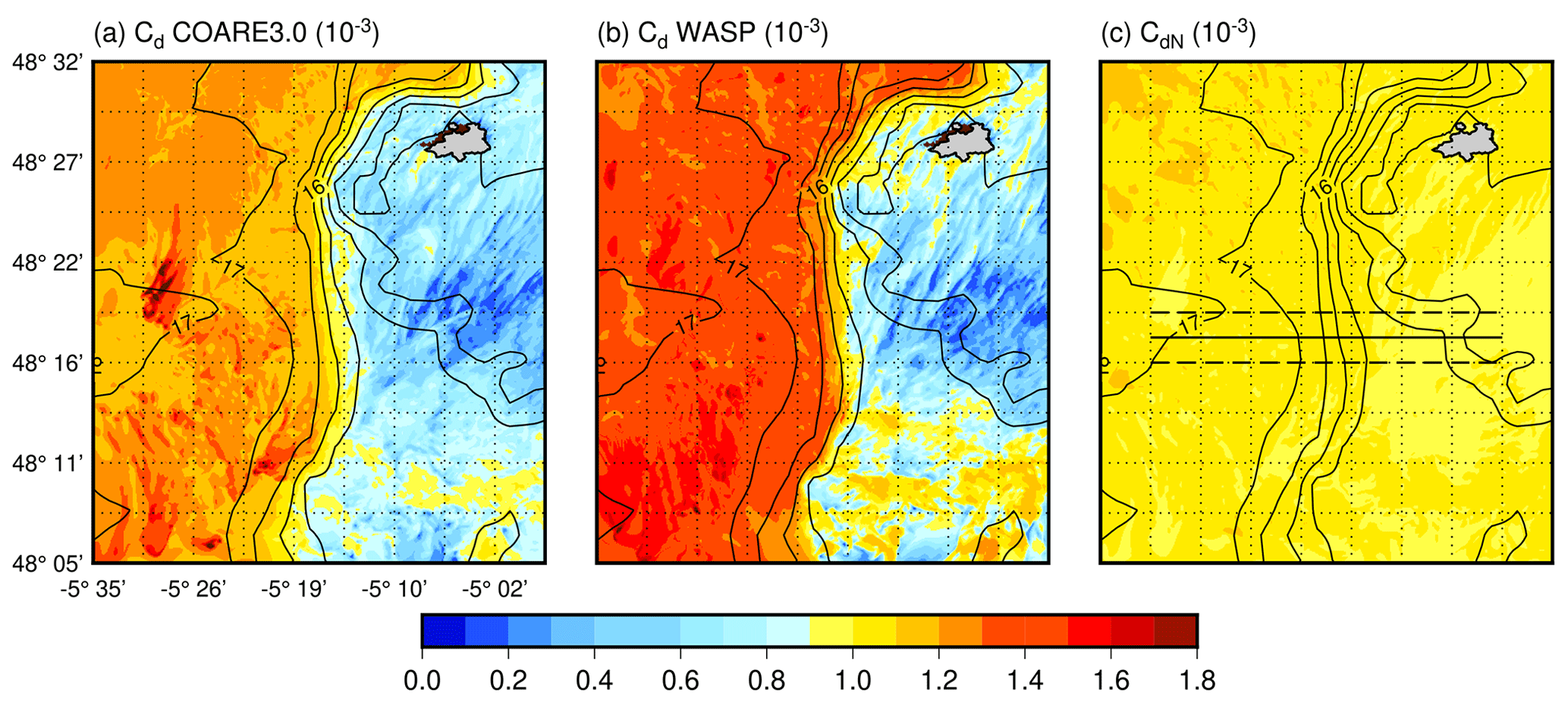
Figure 7 compares the SST, the difference between the SST and the air temperature, the drag coefficient, and the momentum flux along a 35 km profile across the front (see Fig. 8c), from the warm side to the cold side. The decrease in the SST from 17.5 to 15 ∘C (Fig. 7a) produces a strong change in the surface stratification (SST −Ta in Fig. 7b), which results in a strong decrease in the non-neutral drag coefficient Cd (Fig. 7c) from 1.2 × 10⁻³ to 0.5 × 10⁻³. This induces the corresponding decrease in the momentum flux τ (Fig. 7d). The striking correspondence of the change in non-neutral Cd with the SST front can be appreciated in Fig. 8a for the COARE3.0 parameterisation. The role of this stratification change due to advection across the front in controlling Cd has been established in R2019 and is shown here by the difference between the non-neutral and neutral drag coefficients across the front (Fig. 7c – see also Fig. 8c for a map of the neutral drag coefficient, which is almost homogeneous on the domain). The simulation using WASP rather than COARE 3.0 gives the same results with a small intensification of the contrast between both neutral and non-neutral drag coefficients across the front (Figs. 7c and d, 8a and b), in line with slightly higher values of the neutral Cd by weak winds, Fig. 1. In this weak wind situation with a strong gradient of surface stratification, WASP behaves similarly to COARE3.0 in reproducing the decrease in turbulent stress from the warm side to the cold side of the SST front.
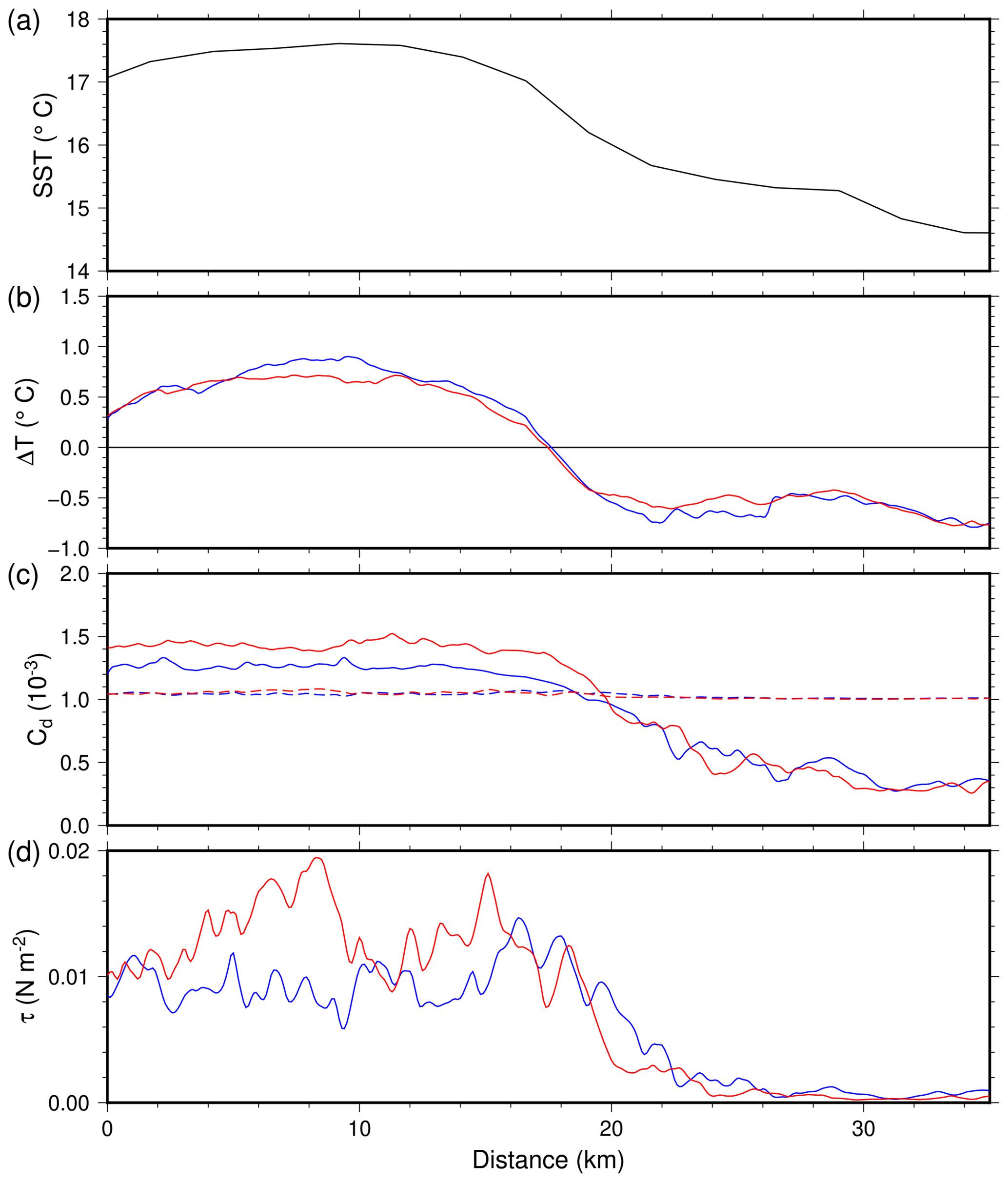
Figure 7Mean values of the SST (a), ΔT = SST −Ta (b), non-neutral drag coefficient (solid) and neutral drag coefficient (dashed) (c), and turbulent stress (d) at 12:00 UT on 2 September 2011 on the Iroise Sea across the SST front, with COARE3.0 (blue) and WASP (red) parameterisations.
3.2 Moderate to strong wind conditions with waves: a Mediterranean Sea case
The western Mediterranean region is regularly affected by heavy precipitation events (HPEs) that are characterised by a large amount of rainfall over a small area in a very short time (typically more than 100 mm in less than 1 d; Ducrocq et al., 2014; Khodayar et al., 2021). These events regularly lead to flash flooding that is a major threat in the area, as it often causes severe damage and in some cases casualties (e.g. Llasat et al., 2013). At a low level, strong winds with high SST as generally encountered in autumn govern heat transfer, which moistens and warms the air parcel, thus increases the instability, and finally intensifies the convection (e.g. Stocchi and Davolio, 2017; Rainaud et al., 2017; Senatore et al., 2020). The SST fine-scale structures and fronts in the Mediterranean are also known to play a role in low-level wind convergence (Meroni et al., 2018, 2020), which is a key triggering mechanism for deep convection and HPEs at sea. Several case studies using kilometre-scale atmospheric models also showed that taking into account the modulation of the surface roughness by the waves can slow down the low-level flow, shifting the convergence lines and/or modifying the spreading of the cold pool formed below the convective system by precipitation evaporation (e.g. Thévenot et al., 2016; Bouin et al., 2017).
The WASP parameterisation has already been tested with and without wave effect by Sauvage et al. (2020, hereafter S2020) on a HPE occurring in mid-October 2016 in south-eastern France. The wave parameters used as input of the parameterisation came from the wave model WW3 v5.16 in forced or coupled mode. In this case, the wave impact on the surface roughness reduces the low-level wind speed of more than 1 m s−1 over a large area and leads to a displacement of the HPE of 40 km towards sea. Since the sensitivity of the wave impact within WASP was already investigated in S2020, we use here the same case study and configuration to test the effect of using WASP in the AROME model with respect to the parameterisation ECUME currently used for operational forecasts. We first give a short summary of the configuration used and then present the results of the comparison.
3.2.1 Case study and modelling configuration
The complete description of the case study and the AROME model in the configuration used here is given in S2020.
The AROME domain configuration is the one used operationally at Météo-France and known as AROME-France (Brousseau et al., 2016) with a grid resolution of 1.3 km and 90 η levels with the first level at 5 m a.s.l. To assess the sensitivity of the simulated event to a change in turbulent flux parameterisation, we performed two identical sets of simulations using either ECUME or WASP with wave forcing from an offline WW3 simulation. Each set was composed of forecast simulations starting at 00:00 UTC on the 12, 13, and 14 October from AROME operational analyses and lasting 42 h. Hourly boundary conditions were sourced from the ARPEGE operational forecasts (Courtier et al., 1991) except for the SST, which came from the global daily analysis of the Mercator Ocean International (∘ resolution, PSY4/GLO12 system, Lellouche et al., 2013).
The situation at a low level is characterised by a cyclonic circulation that induced a south-easterly flow across the Western Mediterranean Sea and by a strong easterly flow originated from the Southern Alps that triggered large sea-surface heat exchanges over the Ligurian Sea and along the French Riviera due to strong wind (up to 20 m s−1 observed at the Azur buoy; 43.4∘ N, 7.8∘ E) and to large air–sea gradients. The convergence zone between the warm and moist southerly flow and the dry and cold easterly flow was found to trigger convection over the sea. A second convective system, over Hérault in the south of France, was initiated by an orographic uplift and was fed by the easterly flow. Both systems produced large amounts of precipitation.
The Gulf of Lion was initially affected by the rapid easterly flow, producing a young sea with significant wave height (Hs) of up to 6 m and strong air–sea fluxes. As the system moved eastwards with the highest wind intensity, the sea state evolved in time from a well-developed sea to swell in this region. Throughout the event, the French Riviera was affected by strong easterly wind generating wind sea.
3.2.2 Results
The expected impact of parameterisation change from ECUME to WASP on this case study is twofold: first, as in S2020, increasing the mean value of the drag coefficient in the range of the wind speed (7–20 m s−1) and adding variability for a given wind speed should decrease the low-level wind and, second, the turbulent heat fluxes should be lowered with respect to the ECUME parameterisation possibly lowering the convection at sea.
Figure 9 shows that at 14:00 UTC on 13 October (i.e. at the peak of precipitation intensity), the 10 m wind speed actually decreases by 1 to 2 m s−1 over a large area in the Ligurian Sea with WASP. The decrease (and local increase) observed in the Gulf of Lion are due to the westward displacement and enhancement of the convergence zone at sea, as observed in S2020. In the Ligurian Sea which is also the place of strong evaporation, the surface enthalpy flux is significantly decreased by 200–250 W m−2 in the WASP simulation (Fig. 10). These two effects have competing impacts on the convective system all along its lifecycle. In ECUME, the stronger easterly wind tends to displace the convergence zone westwards. But, progressively, the larger heat fluxes lead to a more intense convective system at sea. It induces the development of a well-marked cold pool below the system that reinforces the convergence line and pushes it eastwards. As a result of these competing effects, there is no shift in the precipitation area at sea between WASP and ECUME simulations, conversely to what was obtained when comparing simulations done using WASP with and without wave effect in S2020. The convergence and convective system are more stationary, and the intense rainfall patch is thinner but the maximum amount of rainfall is quite similar, as shown by the accumulated rain amounts between 06:00 and 12:00 UTC and between 12:00 and 18:00 UTC on 13 October (Fig. 11). For precipitation that hit the Hérault region, we found a small decrease in the rainfall intensity with WASP, in particular during the mature phase of the system (Fig. 11b, d), induced by the lower warming and moistening of the easterly low-level jet that feeds the convective system.
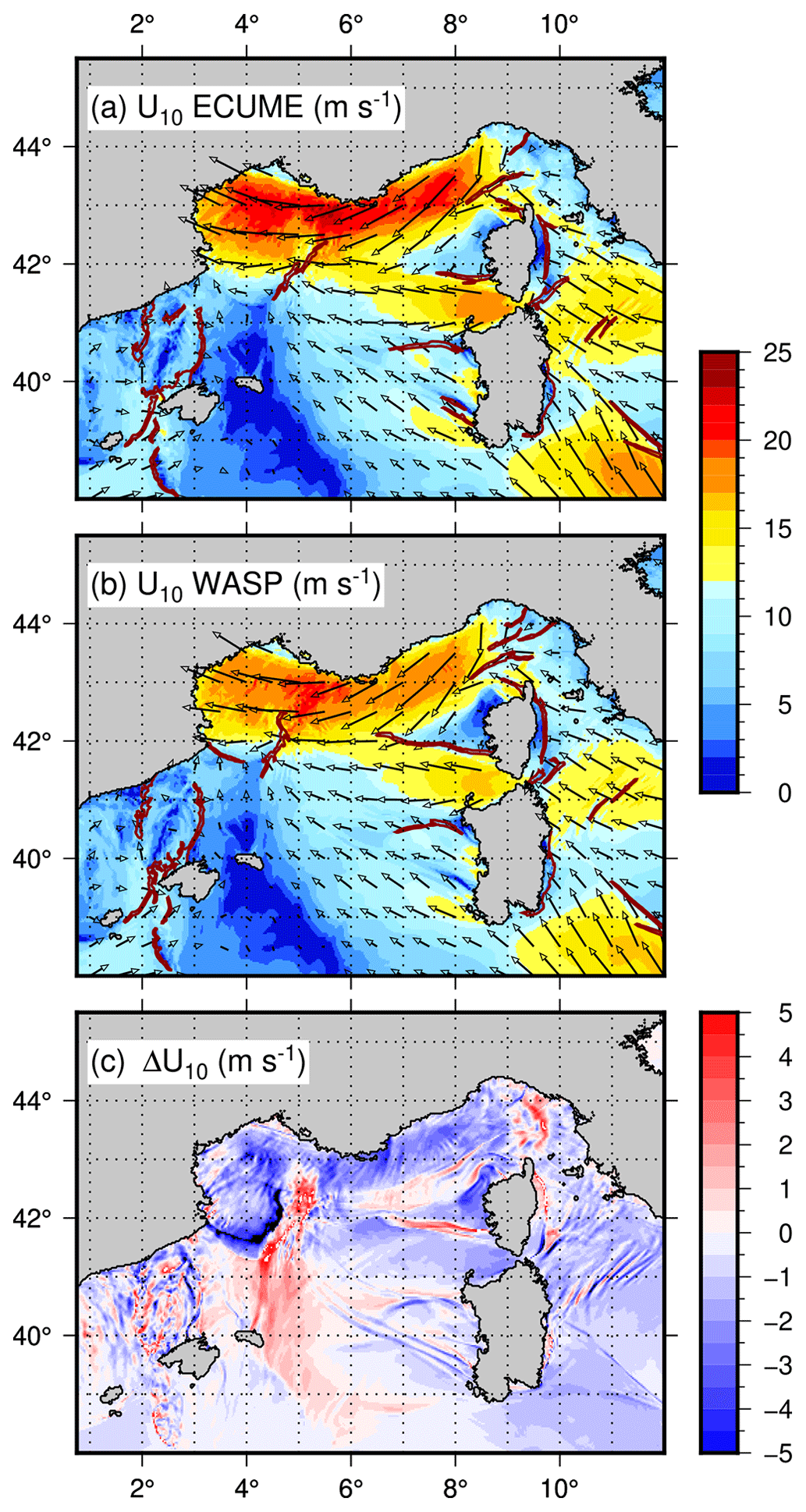
Figure 9Maps of the 10 m wind in the ECUME (a) and WASP forced simulation (b) and difference WASP – ECUME (c) at 14:00 UTC on 13 October 2016. The main convergence area is shown with dark red lines (threshold 10−3 s−1).
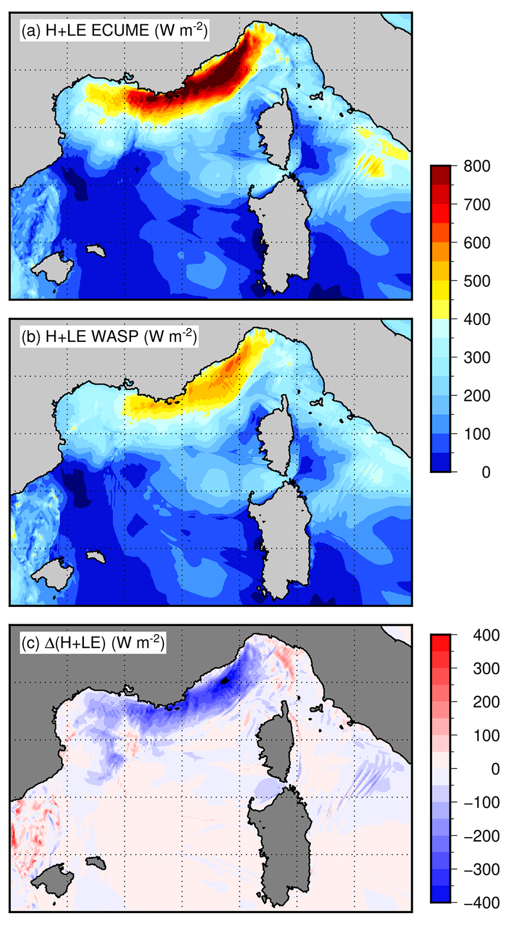
Figure 10Maps of the enthalpy flux in the ECUME (a) and WASP forced simulation (b) and difference WASP − ECUME (c) at 14:00 UTC on 13 October 2016.
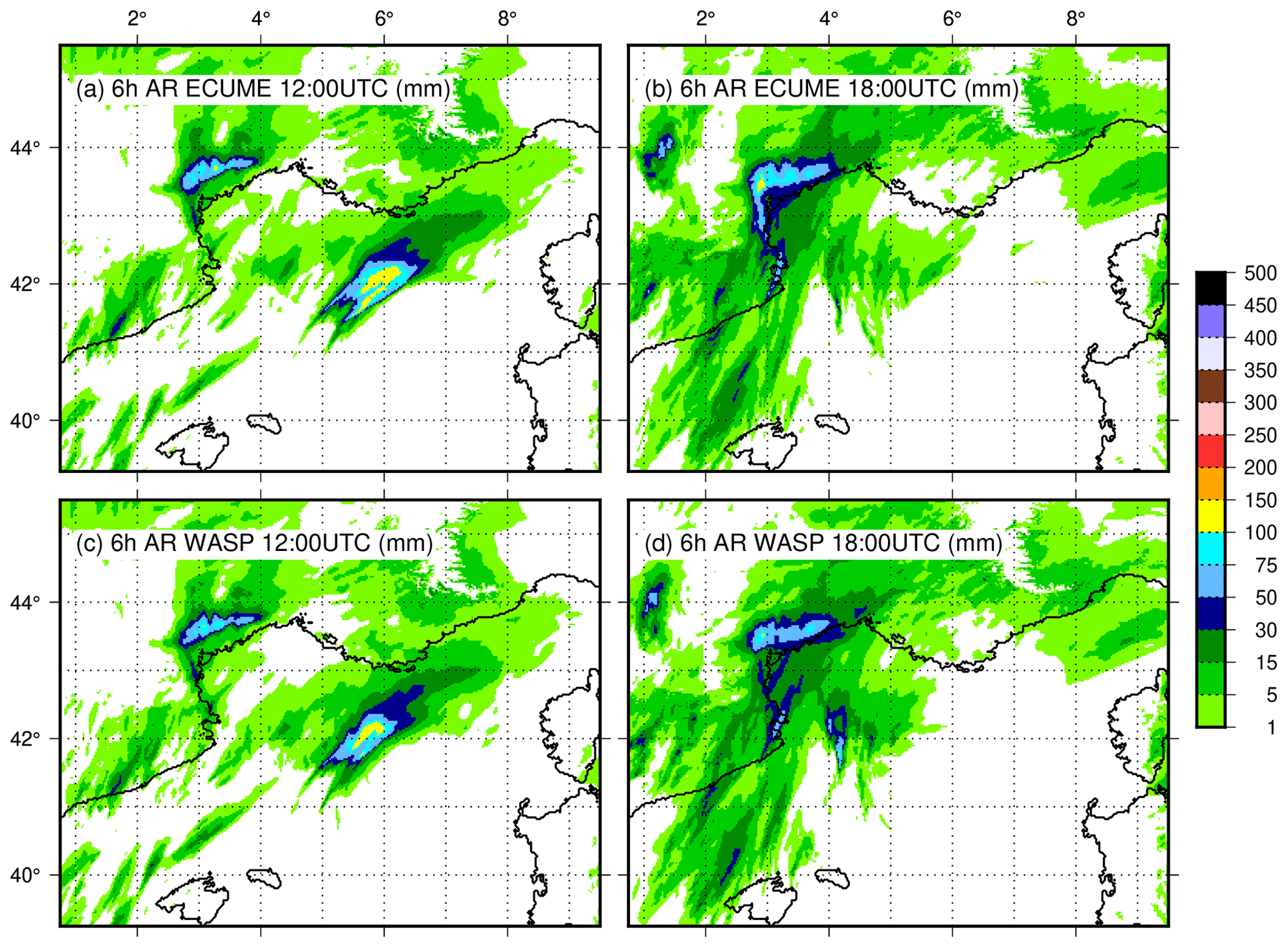
Figure 11Maps of the 6 h accumulated rain in the ECUME (a, b) and WASP forced simulations (c, d) at 12:00 (a, c) and 18:00 UTC (b, d) on 13 October 2016.
The WASP parameterisation used here forced by realistic sea states produced by a WW3 simulation gives results very comparable to the operational simulation. The predictability of the event was good in general, especially concerning the precipitation over the Hérault region, and WASP enables us to obtain similar results with a more realistic sea-surface roughness representation.
3.3 Extreme wind conditions: tropical cyclone
WASP is designed to ensure the representation of the variability due to the wave growth and the saturation of the drag coefficient in case of cyclonic winds. The values of the transfer coefficient for heat are reasonably constrained by the observations for winds up to 20 m s−1, but between 20 and 60 m s−1 observations are too sparse for a robust fit. Case studies of tropical cyclones can help to validate indirectly the values chosen for the drag and heat transfer coefficients in the wind speed range with no observations or observations with large uncertainties.
3.3.1 Case study and modelling configuration
To test the sensitivity to the turbulent fluxes, we used the current operational configuration of AROME for the forecast of the tropical cyclones in the Indian Ocean (AROME IO hereafter; Bousquet et al., 2020). AROME is used over a large domain centred at 50∘ E covering Madagascar and the Mozambique Channel. The horizontal resolution is 1.3 km with 90 vertical levels. It is coupled every 300 s with an oceanic 1D model based on the development of Gaspar et al. (1990), with a prognostic equation of the turbulent kinetic energy with a 1.5-order closure. This 1D ocean model is initialised by the Mercator Océan International global operational forecasts (1 h average) available 6 hourly with a resolution of ∘ (Lellouche et al., 2018). The surface turbulent fluxes are parameterised by ECUME in the control run (operational configuration) and with WASP without waves in the sensitivity experiment. The case studies chosen for this validation are those of the cyclonic season 2021–2022, with a focus on Batsirai. Batsirai developed at the end of January 2022, reached category 4 on the 2 February 2022 right before hitting Réunion Island, and slightly weakened to category 3 before landing on the eastern coast of Madagascar, where it caused a lot of damage. Simulations of Batsirai started at 00:00 and 12:00 UTC on 3 February 2022, and 00:00 UTC on 4 February 2022 and lasted 72 h. The profiles shown in Fig. 12 are composites built from these three runs and ranges of 39 h for the first initial time, 27 h for the second one, and 15 h for the last one. The output time is 15:00 UTC on the 4 February matching the time of the Sentinel-1A SAR data at 15:03 UTC on the same day. These SAR high-resolution wind products are obtained from the IFREMER/CyclObs database and produced with the SAR wind processor co-developed by IFREMER and CLS (Mouche et al., 2017).
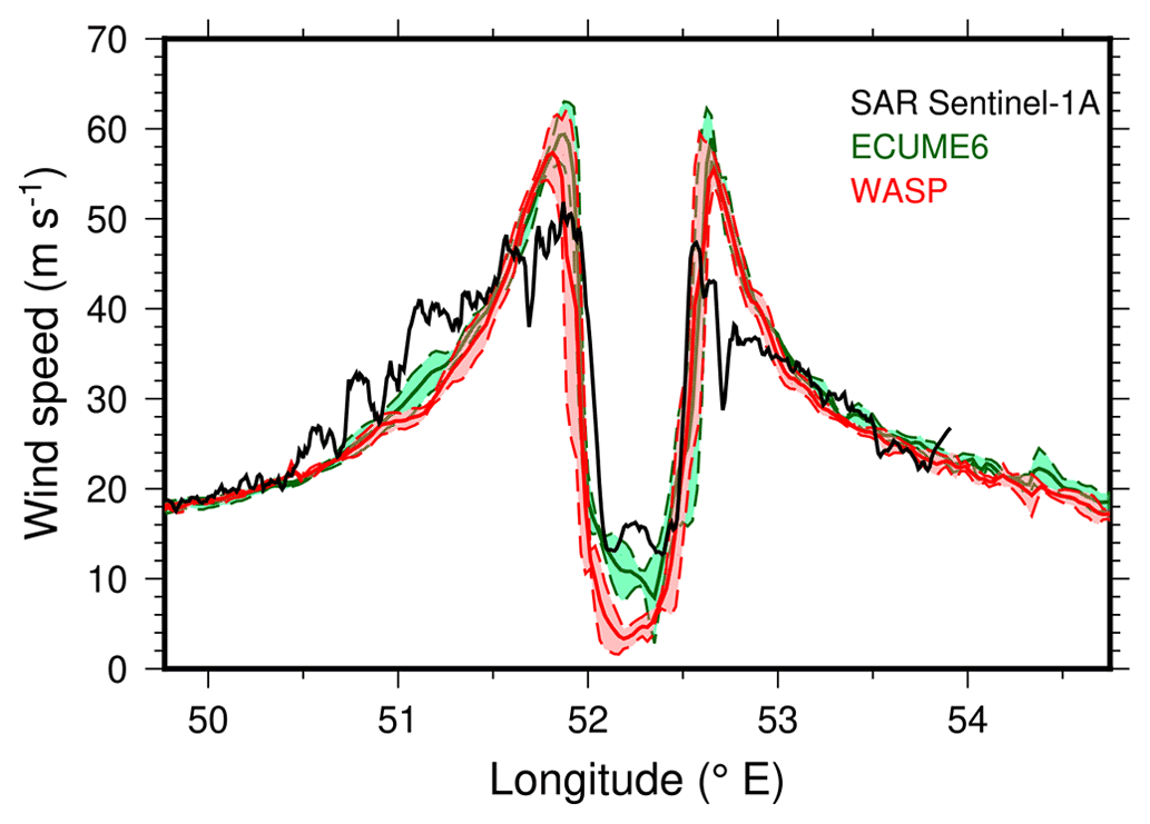
Figure 12West–east composite profiles of U10 (m s−1) across the AROME IO simulations of Batsirai at the time of SAR Sentinel-1A measurements (15:00 UTC on 4 February) from operational runs at three different initial times. The solid line represents the mean value and the dotted lines the standard deviation.
3.3.2 Results
The scores based on the comparison of the minimum of sea-level pressure (SLPmin) and surface maximum wind (Vmax) produced by the simulations with those of the best tracks have been produced for three major cyclones of the 2021–2022 cyclonic season in the southern Indian Ocean (Fig. 13). The best track (BT) is the result of the objective analysis of the Regional Specialised Meteorological Centre for Tropical Cyclones of La Réunion and is regarded as the reference in this study. The scores used here aggregate the outputs of about 25 runs with different initial times for every cyclone, either from IFS, AROME IO using ECUME, or AROME IO using WASP. AROME IO with ECUME compares well with the BT at forecast ranges up to 12 h but overestimates the cyclone intensity (lower SLPmin and higher Vmax) at longer ranges, even more so at increasing forecast ranges, while IFS overall underestimates the cyclone intensity. AROME IO with WASP underestimates Vmax in the first 12 h (probably due to the effect of the initial conditions) but gives the closest values of SLPmin and Vmax to the BT for the forecast ranges longer than 12 h. For the case of Batsirai where SAR observations are available close to its peak of intensity, direct comparisons of composite 10 m wind speed with SAR surface wind show that the wind speed along a profile across the cyclone is slightly better represented using WASP than ECUME (Figs. 12 and 14).
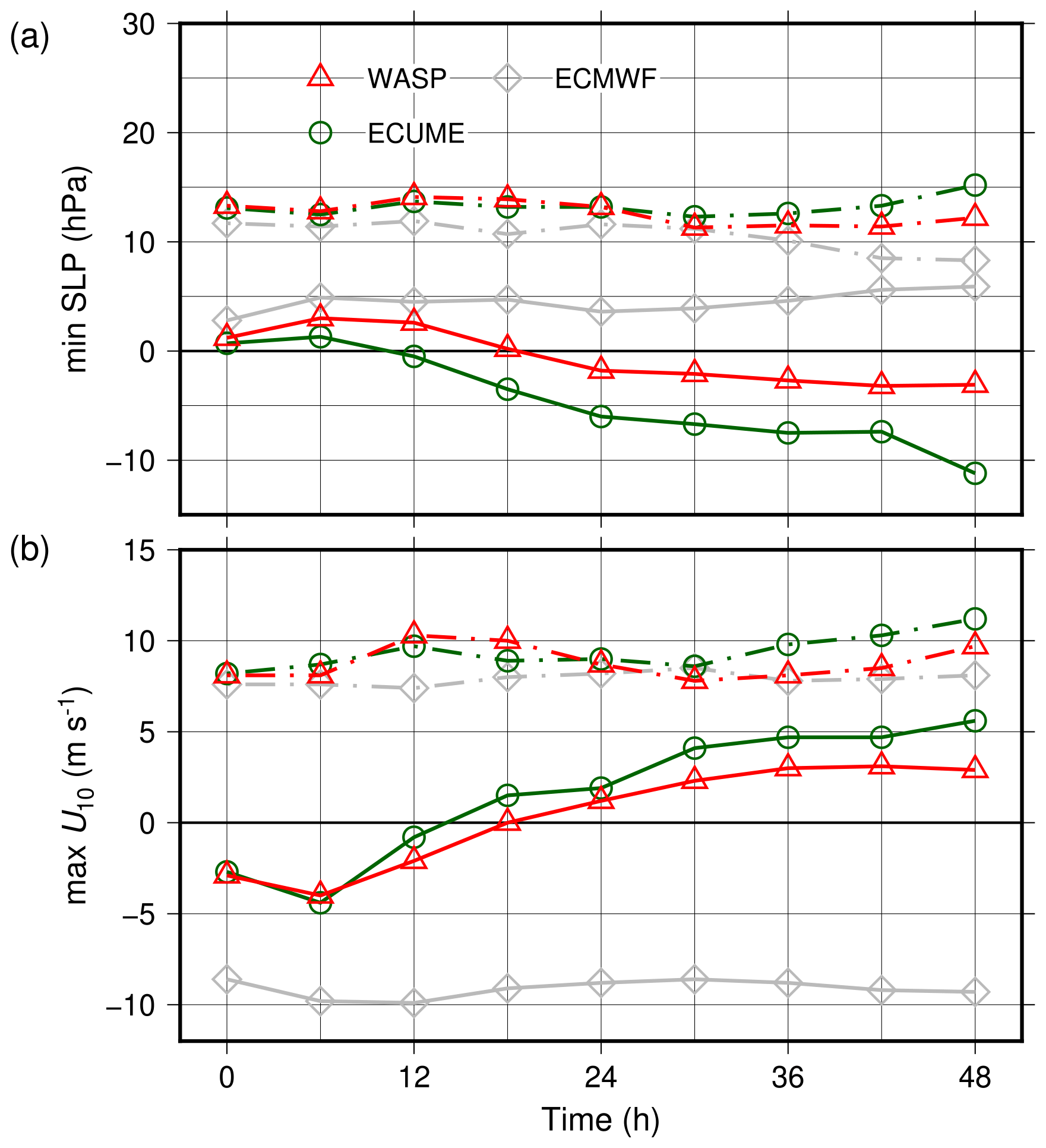
Figure 13Mean bias (solid line) and RMSE (dot–dashed line) for the Batsirai, Emnati and Dumako simulations using AROME IO with ECUME (dark green, circles) or WASP (triangles, red) and IFS (diamonds, grey) for SLPmin (a) and Vmax (b).
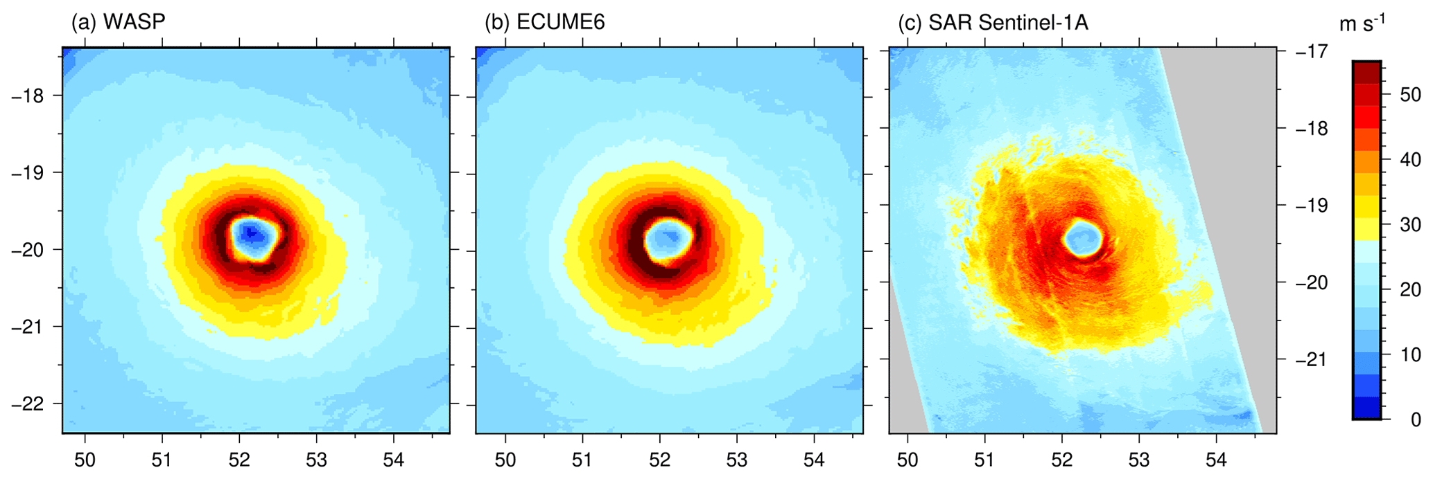
Figure 14Maps of the 10 m wind speed close to the time of maximum intensity in the TC Batsirai, as simulated with AROME IO using ECUME (a), WASP (b), and in the Sentinel-1A SAR product (c). Simulation products shown here are composites from outputs at 15:00 UTC of three simulations starting at 00:00 UTC on 3 February, at 12:00 UTC on 3 February, and at 00:00 UTC on 4 February 2022. The time of the SAR observations is 15:03 UTC on 4 February 2022.
Simplified, axisymmetric representations of tropical cyclones make the maximum potential intensity directly depend on the ratio of the enthalpy transfer coefficient (Ck, analogous to Ce here) by the drag coefficient. The minimum value of this ratio, , able to produce maximum surface winds of 45 m s−1 or more as currently observed in cyclones of category 5, was thought to be 0.75 (Emanuel, 1995). These considerations, however, have been contradicted by in situ and wave tank observations: increasing surface winds up to 40 m s−1 are consistent with a slow but continuous decrease in the ratio down to 0.5 (Powell et al., 2003; Haus et al., 2010). Recently, simulations based on realistic, high-resolution numerical models showed that the Cd and Ck values leading to cyclone intensities close to observations and compatible with observations of turbulent fluxes in strong wind actually result in ratio close to 0.5 (Green and Zhang, 2013, 2014; Nystrom et al., 2020). In such a respect, the ratio of enthalpy and drag coefficient obtained in WASP stays between 0.4 and 1.0 for wind speeds between 10 and 60 m s−1 (Fig. 15). It constitutes a good tradeoff between the continuous decreasing values given by COARE 3.0 and COARE 3.5 and the values of ECUME increasing probably unrealistically up to 1.5 for surface winds of 60 m s−1, and it encourages us to test in a more comprehensive way the use of WASP for tropical cyclone prediction.
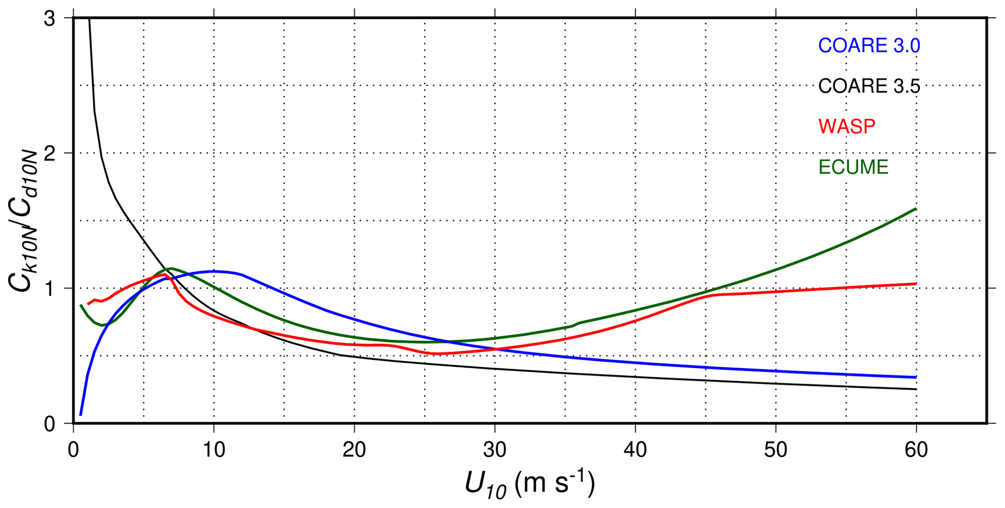
Figure 15Ratios of the neutral enthalpy transfer coefficient and drag coefficient with respect to 10 m wind speed for different parameterisations (COARE3.0, Fairall et al., 2003; COARE3.5, Edson et al., 2013; WASP; and ECUME, Roehrig et al., 2020).
3.4 Climate-scale simulation
The sensitivity of climate-scale runs to the turbulent flux parameterisation was tested in climate mode using the CNRM-CM model (Roehrig et al., 2020).
3.4.1 Configuration
The test was carried out in an atmospheric simulation where SST are prescribed on a monthly basis over the 1979–2014 period following the Atmospheric Model Intercomparison Project (AMIP) protocol. The reference simulation for which the air–sea fluxes are calculated using the ECUME parameterisation has been published in the Couple Model Intercomparison Project Phase 6 (CMIP6) database and is extensively described and assessed in Roehrig et al. (2020). Here we only provide minimal information on this configuration: the horizontal resolution is close to 1.4∘, and there are 91 vertical levels in the atmosphere with the first level at 10 m. To test the WASP parameterisation, a sensitivity experiment was performed where WASP instead of ECUME is activated over the same 35 years (1979–2014).
3.4.2 Results
Mapping the differences between surface parameters and fluxes obtained with the WASP and ECUME parameterisations shows an overall impact of the change in transfer coefficients. In the regions of high annual mean values of heat fluxes, namely the intertropical basins, the impact of such parameterisation changes was explored by Torres et al. (2019). In the present study, CeN in WASP is higher than in ECUME for 10 m wind speed below 8 m s−1 and lower for 10 m wind speed above 8 m s−1. This results in higher evaporation in the intertropical basins (Fig. 16a, b) with annual mean values in the region between 20∘ S and 20∘ N of 121.7 W m−2 with ECUME and 123.2 W m−2 with WASP. With respect to the interannual variability over 36 years, this change is not significant (at 95 % uncertainty with a Student's t test). It nevertheless results in overall higher humidity on the ocean (+0.21 g kg−1 – not significant; Fig. 16c). Also, stronger precipitation (below the significance level) is obtained along the intertropical convergence zone (ITCZ; Fig. 16d, +0.65 mm d−1). Outside the intertropical region, using WASP rather than ECUME results in lower specific humidity near the surface (Fig. 16c) and less precipitation (Fig. 16d). These results are qualitatively similar to those of Torres et al. (2019); see for instance their Figs. 4–2 for the difference between their simulations AREF and ACTN.
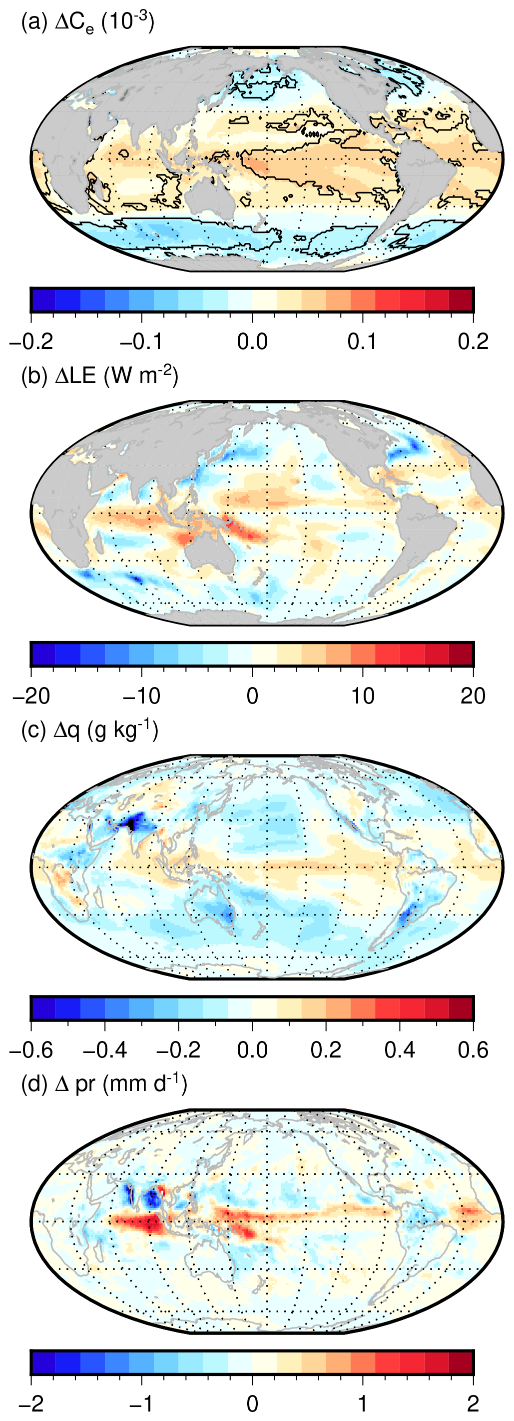
Figure 16Maps of the annual mean differences for Ce (a), LE (b), q at the lowest atmospheric level (c), and daily precipitation pr (d) between WASP and ECUME in AMIP simulations over the period 1979–2014. The black lines indicates the zones where the difference is significant with respect to the interannual variability (Student's t test at 95 % uncertainty).
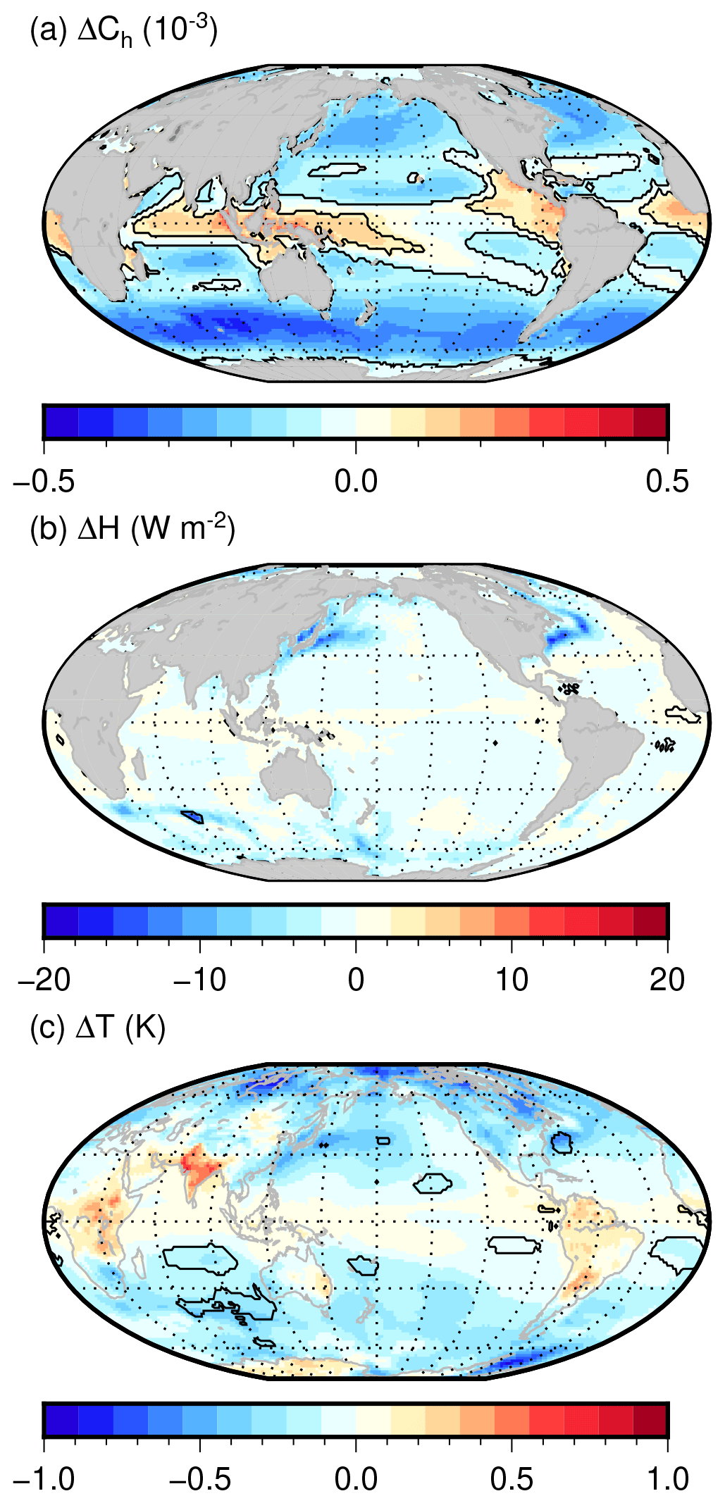
Figure 17Maps of the annual mean differences for Ch (a), H (b), and T at the lowest atmospheric level (c) between WASP and ECUME in AMIP simulations over the period 1979–2014.
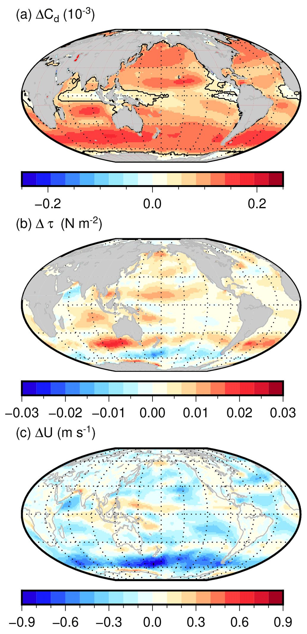
Figure 18Maps of the annual mean differences for Cd (a), τ (b), and U at the lowest atmospheric level (c) between WASP and ECUME in AMIP simulations over the period 1979–2014.
The lowest-level atmospheric temperature annual mean increases slightly in the intertropical regions and decreases at midlatitudes (mostly not significant, Fig. 17c). This is due to the strong changes in the sensible and latent heat transfer coefficient in WASP (overall significant, Figs. 17a, 16a) which impact the sensible and latent heat fluxes, through a decrease at midlatitudes and an increase in the intertropical band (not significantly, Figs. 17b, 16b). Note that stronger decrease on the western boundary energetic areas is partly due to a larger decrease in the heat transfer coefficients by stronger wind. Finally, the neutral drag coefficient is higher in WASP than in ECUME, whatever the wind speed below 19 m s−1 (Fig. 18a). The wind stress is higher everywhere at the sea surface except locally in the Arabic Sea and in the Southern Ocean (Fig. 18a, b, N m−2). This results in an overall decrease in the wind speed, with a stronger effect in the Southern Ocean where the increase in the drag coefficient is the strongest (Fig. 18c, −0.09 m s−1). Overall, testing WASP in a climate-scale configuration does not alter significantly the mean climate simulated. No significant change is obtained except for a slight increase in the precipitation in the ITCZ and a slight cooling and drying effect outside the ITCZ. Further tests should be done in ocean-coupled mode to assess the coupling feedback that could arise when switching to WASP air–sea flux parameterisation.
The WASP bulk parameterisation for surface turbulent fluxes has been built based on existing, reliable parameterisations like COARE 3.0 (Fairall et al., 2003), COARE 3.5 for the momentum flux (Edson et al., 2013), and ECUME (Belamari, 2005; Roehrig et al., 2020). It does not necessarily represent an improvement towards a more accurate representation of turbulent fluxes but rather combines the possibility of representing the effect of the wave growth on the wind stress with transfer coefficients close to field observations at every range of wind speed. It has been developed in the SURFEX v8.1 surface model (Masson et al., 2013) and will be distributed as part of the next official SURFEX release (v9). In the present study, we assess its behaviour in several case studies performed with the different atmospheric models in use at Météo-France that can be coupled with SURFEX. It proves to perform reliably with respect to existing parameterisations in various conditions of wind and heat transfer and to enable an accurate representation of several surface processes. In the case of the Ushant SST front (Redelsperger et al., 2019), the sharp change in stratification along the low-level flow from the warm side to the cold side of the front is well reproduced and leads to a strong decrease in the momentum flux. As a result, the turbulence on the cold side of the front is decoupled between the upper MABL and the surface and the surface wind is reduced. In the HPE that occurred in the Western Mediterranean in October 2016, the change in parameterisation affects the strong, moist low-level flow leading to change in heavy precipitation mainly through dynamical effects. Representing the surface fluxes by WASP rather than ECUME increases the surface roughness and decreases the turbulent heat fluxes. It results in a slightly less intense but more stationary convective system at sea without a significant impact on the precipitation forecast. Validating the parameterisation in cyclonic conditions is an important step towards its use for operational forecast. In the present case, it also helped to adjust the heat transfer coefficients above 20 m s−1, where observations provide no constrain anymore. Several case studies in the south-west Indian Ocean basin showed that the intensity of cyclones is slightly reduced with respect to ECUME, mainly due to the decrease in the enthalpy transfer coefficient in case of strong and cyclonic winds. Finally, testing the impact of the change on a climatic atmosphere-only simulation gives results consistent with existing studies. The combined effects of the changes in the wind stress and heat fluxes enhance moisture extraction and precipitation in the intertropical zone, whereas a lower atmosphere is drier and cooler at midlatitudes. This work is a first step towards further development of the parameterisation of both momentum and turbulent heat fluxes. Ongoing work aims at refining the representation of the variability in the fluxes possibly due to sea-state variations, including the effects of wave breaking and the effect of sea spray on the momentum and heat fluxes. Indeed, the effect of sea spray, though likely significant for both the momentum and heat transfer in breaking conditions, is not considered in WASP. Recent and ongoing studies aim at building droplet source functions more consistent with the (few) existing observations for large droplets, meant to affect the turbulent fluxes (Bruch et al., 2021), and the corresponding parameterisation of their impact on the fluxes following Bao et al. (2011).
A1 Transfer coefficients
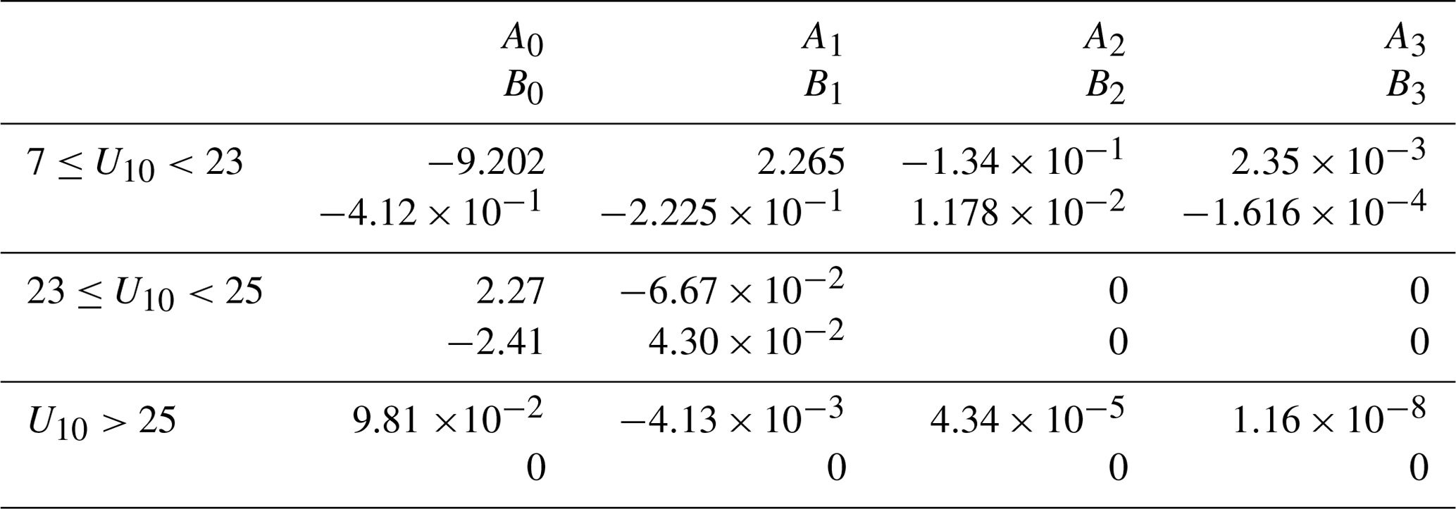
In WASP, the Charnock parameter α is defined differently depending on the wind speed range, as follows:
-
10 m wind speed U10 below 7 m s−1 is a power of U10 – , where a=0.7 and b=−2.52;
-
when U10 is above 7 m s−1, the dependency on wave age is introduced and is defined as α=AχB, where A and B are polynomial functions of U10.
as detailed in Table A1.
Thus, the dependency of the Charnock parameter and the decrease in the drag coefficient under very strong wind conditions are represented, and the WASP parameterisation, unlike those based on wave-age Charnock parameters, is suitable for very high wind speeds.
Table A1Coefficients of the polynomial functions defining the WASP Charnock parameter depending on the wind speed.
A2 Stability functions
The stability functions for momentum and heat fluxes are taken as in Beljaars and Holtslag (1991), modified to be implemented in the COARE 3.0 algorithm (Fairall et al., 2003). In unstable conditions, the stability function for momentum is as follows:
with . In conditions of free convection, it is
with . In stable conditions, it is
with . The stability function for heat or humidity is defined as follows:
with . In conditions of free convection, it is defined as follows:
with . In stable conditions, it is defined as follows:
with .
Table B1Eddy covariance datasets used for fitting the neutral transfer coefficients in the wind speed range 0–20 m s−1. All these measurements except CBLAST low (research platform, RP, FLIP) were made on board ships.
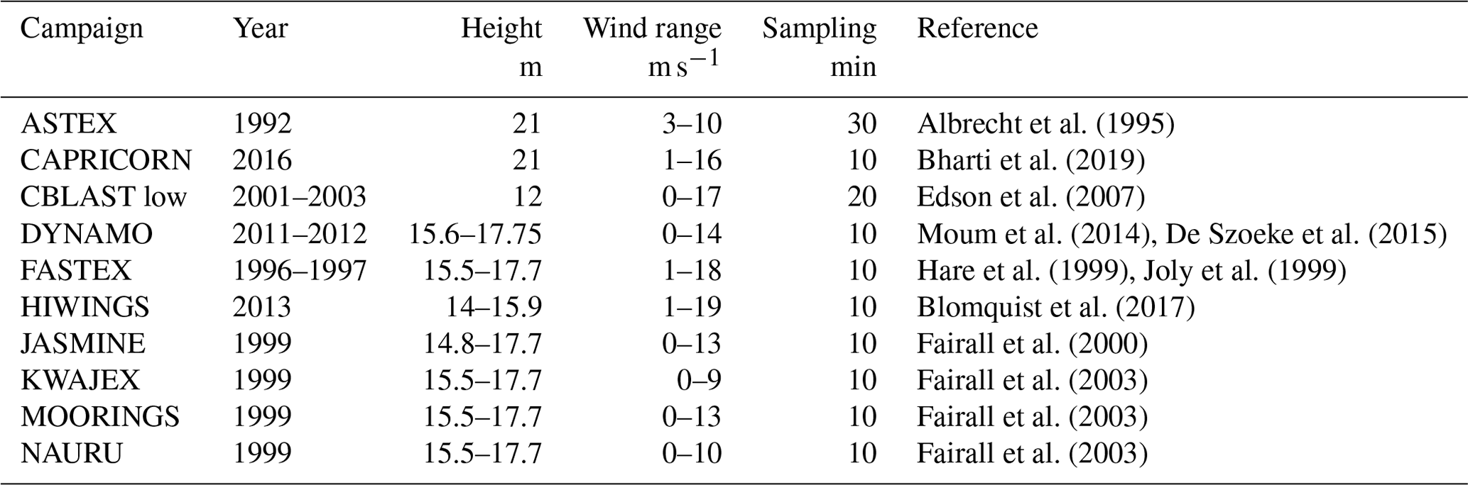
Table B2Additional EC datasets used for fitting the neutral transfer coefficients in the wind speed range 0–30 m s−1.
* indicates that measurements of enthalpy fluxes are available.
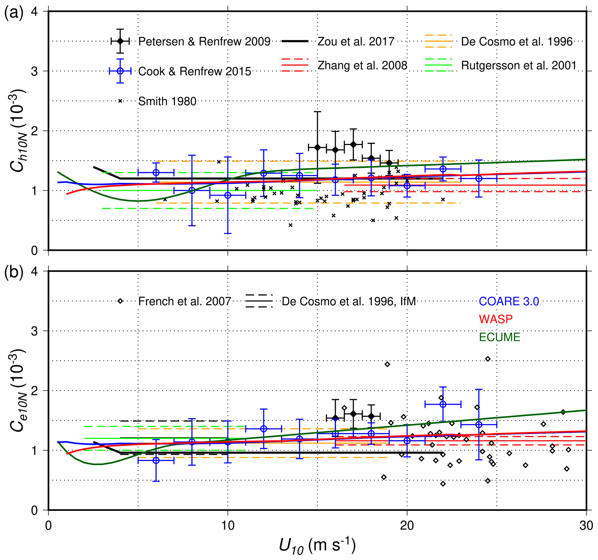
Figure B1Sensible (a) and latent (b) heat transfer coefficients with respect to 10 m wind speed for different parameterisations (COARE3.0, Fairall et al., 2003; ECUME, Roehrig et al., 2020; and WASP) in comparison with additional observations (see Table B2) up to 28 m s−1.
Table B3Additional, indirect datasets used for fitting the neutral transfer coefficients in the wind speed range above 30 m s−1.
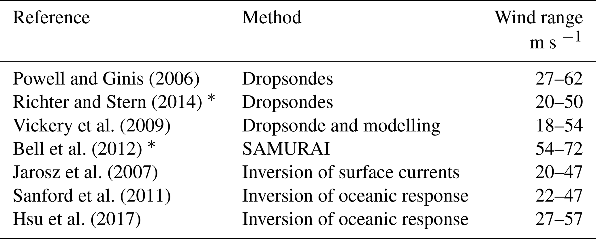
* indicates that measurements of enthalpy fluxes are available.
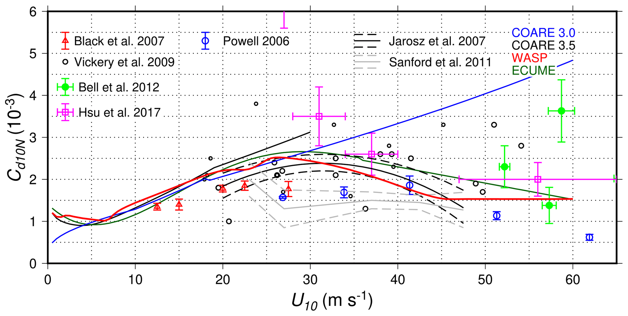
Figure B2Neutral drag coefficient with respect to 10 m wind speed for different parameterisations (COARE3.5, Edson et al., 2013; COARE3.0, Fairall et al., 2003; ECUME, Roehrig et al., 2020; and WASP) and detail of observations up to 60 m s−1 (see Tables B2 and B3).
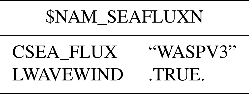
C1 WASP without wave impact
Table C1SURFEX name list (EXSEG1.nam) parameters used for using WASP without wave impact.
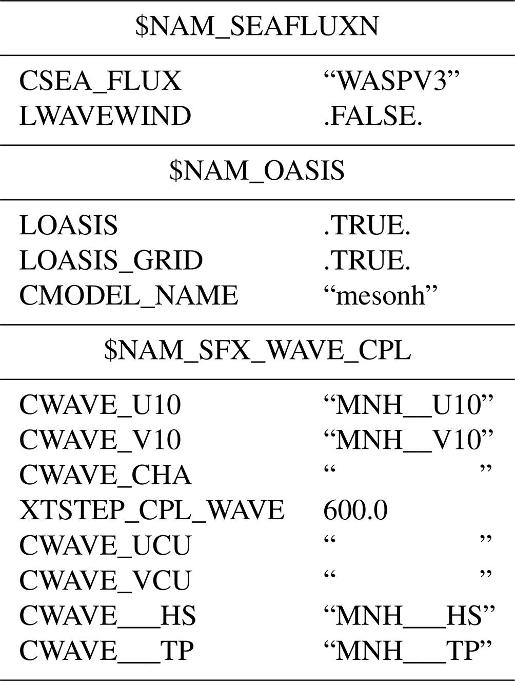
C2 WASP with wave impact
Table C2SURFEX name list (EXSEG1.nam) parameters used for using WASP with wave coupling, with a coupling frequency of 600 s.1
The newly developed code will be included in the next official version of SURFEX v9.0. The complete code of SURFEX v8.1 including WASP and the WASP subroutines is available at https://doi.org/10.5281/zenodo.4557378 (Bouin, 2021); the data used to tune the transfer coefficients are available by contacting Christopher W. Fairall (NOAA Physical Science Division) or James B. Edson (U. Conn. Marine Sciences). The official release of SURFEX v8.1 offline is available at https://www.umr-cnrm.fr/surfex/spip.php?rubrique141 (last access: 10 December 2023). The ARPEGE-Climat model is only available to registered users for research purposes. The access to the AROME code is ruled by the first Memorandum of Understanding of the ACCORD consortium (http://www.accord-nwp.org, last access: 10 December 2023). For non-commercial research purposes, AROME can be distributed upon signature of a licence agreement (see http://www.accord-nwp.org/?ACCORD-MoU-2021-2025, last access: 10 December 2023, for conditions). Data can be accessed upon request. The output parameters of the simulations used to validate WASP (Figs. 7 to 18) and the data of the Lion buoy used to compare the wave effects in Fig. 4 are available at https://doi.org/10.5281/zenodo.6783319 (Bouin, 2022). The SAR product was obtained from Ifremer/CyclObs and produced with SAR wind processor co-developed by IFREMER and CLS and can be accessed here: https://cyclobs.ifremer.fr/app/archive/2022/SI/sh082022 (last access on 30 June 2022; Mouche and Archer, 2023). The best track data have been extracted from the best track database of the Direction Régionale de l’Océan Indien (DIROI) of Météo-France. These data are shared with the IBTrACS database (https://www.ncdc.noaa.gov/ibtracs/, last access: 20 December 2023; DOI: https://doi.org/10.25921/82ty-9e16, Knapp et al., 2010, 2018) after a subjective reanalysis by the DIROI forecasters at the end of each TC season.
MNB designed and implemented the WASP parameterisation and performed the Iroise case study. CLB and CS designed and ran the Mediterranean case study. SM designed and performed the tropical cyclones case studies. AV designed and performed the climate-scale simulation. All authors contributed to the writing and revising of the paper.
The contact author has declared that none of the authors has any competing interests.
Publisher’s note: Copernicus Publications remains neutral with regard to jurisdictional claims made in the text, published maps, institutional affiliations, or any other geographical representation in this paper. While Copernicus Publications makes every effort to include appropriate place names, the final responsibility lies with the authors.
The authors acknowledge the Pôle de Calcul et de Données Marines for the DATARMOR facilities (storage, data access, computational resources). We are also grateful to Christopher W. Fairall for providing field measurements. We thank Alexis Mouche and Olivier Archer (LOPS) and CLS for providing the SAR products in the framework of the Ifremer/CyclObs project.
This paper was edited by Olivier Marti and reviewed by Christopher Fairall and one anonymous referee.
Albrecht, B. A., Bretherton, C. S., Johnson, D., Scubert, W. H., and Frisch, A. S.: The Atlantic stratocumulus transition experiment – ASTEX, B. Am. Meteorol. Soc., 76, 889–904, 1995. a
Andreas, E. L.: Spray stress revisited, J. Phys. Oceanogr., 34, 1429–1440, 2004. a
Bao, J.-W., Fairall, C. W., Michelson, S., and Bianco, L.: Parameterizations of sea-spray impact on the air–sea momentum and heat fluxes, Mon. Weather Rev., 139, 3781–3797, 2011. a
Belamari, S.: Report on uncertainty estimates of an optimal bulk formulation for surface turbulent fluxes, Marine EnviRonment and Security for the European Area–Integrated Project (MERSEA IP), Deliverable D, 4, 505 pp., 2005. a, b
Beljaars, A. and Holtslag, A.: Flux parameterization over land surfaces for atmospheric models, J. Appl. Meteorol. Clim., 30, 327–341, 1991. a, b
Beljaars, A. C. M.: The parametrization of surface fluxes in large-scale models under free convection, Q. J. Roy. Meteor. Soc., 121, 255–270, https://doi.org/10.1002/qj.49712152203, 1994. a
Bell, M. M., Montgomery, M. T., and Emanuel, K. A.: Air–sea enthalpy and momentum exchange at major hurricane wind speeds observed during CBLAST, J. Atmos. Sci., 69, 3197–3222, 2012. a, b
Bharti, V., Fairall, C. W., Blomquist, B. W., Huang, Y., Protat, A., Sullivan, P. P., Siems, S. T., and Manton, M. J.: Air-sea heat and momentum fluxes in the Southern Ocean, J. Geophys. Res.-Atmos., 124, 12426–12443, 2019. a
Black, P. G., D'Asaro, E. A., Drennan, W. M., French, J. R., Niiler, P. P., Sanford, T. B., Terrill, E. J., Walsh, E. J., and Zhang, J. A.: Air–sea exchange in hurricanes: Synthesis of observations from the coupled boundary layer air–sea transfer experiment, B. Am. Meteorol. Soc., 88, 357–374, 2007. a, b, c
Blomquist, B. W., Brumer, S. E., Fairall, C. W., Huebert, B. J., Zappa, C. J., Brooks, I. M., Yang, M., Bariteau, L., Prytherch, J., Hare, J. E., Czerski, H., Matel, A., and Pascal, R. W.: Wind speed and sea state dependencies of air-sea gas transfer: Results from the High Wind speed Gas exchange Study (HiWinGS), J. Geophys. Res.-Oceans, 122, 8034–8062, 2017. a
Bouin, M.-N.: WASP turbulent fluxes parameterization for SURFEX 8.0, Zenodo [code], https://doi.org/10.5281/zenodo.4557378, 2021. a
Bouin, M.-N.: Datasets and model outputs used for validating WASP for SURFEX v8.0, Zenodo [data set], https://doi.org/10.5281/zenodo.6783319, 2022. a
Bouin, M.-N., Redelsperger, J.-L., and Lebeaupin Brossier, C.: Processes leading to deep convection and sensitivity to sea-state representation during HyMeX IOP8 heavy precipitation event, Q. J. Roy. Meteor. Soc., 143, 2600–2615, 2017. a
Bousquet, O., Barbary, D., Bielli, S., Kebir, S., Raynaud, L., Malardel, S., and Faure, G.: An evaluation of tropical cyclone forecast in the Southwest Indian Ocean basin with AROME-Indian Ocean convection-permitting numerical weather predicting system, Atmos. Sci. Lett., 21, e950, https://doi.org/10.1002/asl.950, 2020. a
Brousseau, P., Seity, Y., Ricard, D., and Léger, J.: Improvement of the forecast of convective activity from the AROME-France system, Q. J. Roy. Meteor. Soc., 142, 2231–2243, https://doi.org/10.1002/qj.2822, 2016. a
Bruch, W., Piazzola, J., Branger, H., van Eijk, A. M., Luneau, C., Bourras, D., and Tedeschi, G.: Sea-Spray-Generation Dependence on Wind and Wave Combinations: A Laboratory Study, Bound.-Lay. Meteorol., 180, 477–505, 2021. a
Bryan, G. H.: Effects of surface exchange coefficients and turbulence length scales on the intensity and structure of numerically simulated hurricanes, Mon. Weather Rev., 140, 1125–1143, 2012. a
Charnock, H.: Wind stress on a water surface, Q. J. Roy. Meteor. Soc., 81, 639–640, https://doi.org/10.1002/qj.49708135027, 1955. a
Chen, X., Hara, T., and Ginis, I.: Impact of shoaling ocean surface waves on wind stress and drag coefficient in coastal waters: 1. Uniform wind, J. Geophys. Res.-Oceans, 125, e2020JC016222, https://doi.org/10.1029/2020JC016222, 2020. a
Cook, P. A. and Renfrew, I. A.: Aircraft-based observations of air–sea turbulent fluxes around the British Isles, Q. J. Roy. Meteor. Soc., 141, 139–152, 2015. a, b
Courtier, P., Freydier, C., Geleyn, J., Rabier, F., and Rochas, M.: The ARPEGE project at Meteo-France, ECMWF, workshop on numerical methods in atmospheric models, Reading, UK, 9–13, 1991. a, b
DeCosmo, J., Katsaros, K., Smith, S., Anderson, R., Oost, W., Bumke, K., and Chadwick, H.: Air-sea exchange of water vapor and sensible heat: The Humidity Exchange Over the Sea (HEXOS) results, J. Geophys. Res.-Oceans, 101, 12001–12016, 1996. a
Déqué, M., Dreveton, C., Braun, A., and Cariolle, D.: The ARPEGE/IFS atmosphere model: a contribution to the French community climate modelling, Clim. Dynam., 10, 249–266, 1994. a
De Szoeke, S. P., Edson, J. B., Marion, J. R., Fairall, C. W., and Bariteau, L.: The MJO and air–sea interaction in TOGA COARE and DYNAMO, J. Climate, 28, 597–622, 2015. a
Donelan, M. A., Dobson, F. W., Smith, S. D., and Anderson, R. J.: On the dependence of sea surface roughness on wave development, J. Phys. Oceanogr., 23, 2143–2149, 1993. a
Donelan, M. A., Drennan, W. M., and Katsaros, K. B.: The air–sea momentum flux in conditions of wind sea and swell, J. Phys. Oceanogr., 27, 2087–2099, 1997. a
Drennan, W. M., Graber, H. C., Hauser, D., and Quentin, C.: On the wave age dependence of wind stress over pure wind seas, J. Geophys. Res.-Oceans, 108, 8062, https://doi.org/10.1029/2000JC000715, 2003. a
Ducrocq, V., Braud, I., Davolio, S., Ferretti, R., Flamant, C., Jansa, A., Kalthoff, N., Richard, E., Taupier-Letage, I., Ayral, P., Belamari, S., Berne, A., Borga, M., Boudevillain, B., Bock, O., Boichard, J.-L., Bouin, M.-N., Bousquet, O., Bouvier, C., Chiggiato, J., Cimini, D., Corsmeier, U., Coppola, L., Cocquerez, P., Defer, E., Delanoë, J., Di Girolamo, P., Doerenbecher, A., Drobinski, P., Dufournet, Y., Fourrié, N., Gourley, J. J., Labatut, L., Lambert, D., Le Coz, J., Marzano, F. S., Molinié, G., Montani, A., Nord, G., Nuret, M., Ramage, K., Rison, B., Roussot, O., Saïd, F., Schwarzenboeck, A., Testor, P., Van Baelen, J., Vincendon, B., Aran, M., and Tamayo, J.: HyMeX-SOP1, the field campaign dedicated to heavy precipitation and flash flooding in the Northwestern Mediterranean, B. Am. Meteorol. Soc., 95, 1083–1100, https://doi.org/10.1175/BAMS-D-12-00244.1, 2014. a
Edson, J., Crawford, T., Crescenti, J., Farrar, T., Frew, N., Gerbi, G., Helmis, C., Hristov, T., Khelif, D., Jessup, A., Johnson, H., Li, M., Mahrt, L., McGillis, W., Plueddemann, A., Shen, L., Skyllingstad, E., Stanton, T., Sullivan, P., Sun, J., Trowbridge, J., Vickers, D., Wang, S., Wang, Q., Weller, R., Wilkin, J., Williams III, A. J., Yue, D. K. P., and Zappa, C.: The coupled boundary layers and air–sea transfer experiment in low winds, B. Am. Meteorol. Soc., 88, 341–356, 2007. a
Edson, J. B., Jampana, V., Weller, R. A., Bigorre, S. P., Plueddemann, A. J., Fairall, C. W., Miller, S. D., Mahrt, L., Vickers, D., and Hersbach, H.: On the exchange of momentum over the open ocean, J. Phys. Oceanogr., 43, 1589–1610, 2013. a, b, c, d, e, f, g, h, i, j
Emanuel, K. A.: Sensitivity of tropical cyclones to surface exchange coefficients and a revised steady-state model incorporating eye dynamics, J. Atmos. Sci., 52, 3969–3976, 1995. a
Emanuel, K. A.: Tropical cyclone energetics and structure, Atmospheric Turbulence and Mesoscale Meteorology, 8, 165–191, 2004. a
Emanuel, K. A.: 100 years of progress in tropical cyclone research, Meteor. Mon., 59, 15.1–15.68, 2018. a
Fairall, C. W., Hare, J. E., Edson, J. B., and McGillis, W.: Parameterization and micrometeorological measurement of air–sea gas transfer, Bound.-Lay. Meteorol., 96, 63–106, 2000. a
Fairall, C. W., Bradley, E. F., Hare, J. E., Grachev, A. A., and Edson, J. B.: Bulk parameterization of air-sea fluxes : Updates and verification for the COARE algorithm, J. Climate, 16, 571–591, 2003. a, b, c, d, e, f, g, h, i, j, k, l, m, n, o, p
French, J. R., Drennan, W. M., Zhang, J. A., and Black, P. G.: Turbulent fluxes in the hurricane boundary layer. Part I: Momentum flux, J. Atmos, Sci,, 64, 1089–1102, 2007. a, b
Gaspar, P., Grégoris, Y., and Lefevre, J.-M.: A simple eddy kinetic energy model for simulations of the oceanic vertical mixing: Tests at station Papa and Long-Term Upper Ocean Study site, J. Geophys. Res.-Oceans, 95, 16179–16193, 1990. a
Green, B. W. and Zhang, F.: Impacts of air–sea flux parameterizations on the intensity and structure of tropical cyclones, Mon. Weather Rev., 141, 2308–2324, 2013. a
Green, B. W. and Zhang, F.: Sensitivity of tropical cyclone simulations to parametric uncertainties in air–sea fluxes and implications for parameter estimation, Mon. Weather Rev., 142, 2290–2308, 2014. a
Hare, J., Persson, P., Fairall, C., and Edson, J.: Behavior of Charnock’s relationship for high wind conditions, in: Preprints, in: 13th Symp. on Boundary Layers and Turbulence, Dallas, TX, 10–15 January 1999, Amer. Meteor. Soc, 252–255, 1999. a
Haus, B. K., Jeong, D., Donelan, M. A., Zhang, J. A., and Savelyev, I.: Relative rates of sea-air heat transfer and frictional drag in very high winds, Geophys. Res. Lett., 37, L07802, https://doi.org/10.1029/2009GL042206, 2010. a
Hsu, J.-Y., Lien, R.-C., D’Asaro, E. A., and Sanford, T. B.: Estimates of surface wind stress and drag coefficients in Typhoon Megi, J. Phys. Oceanogr., 47, 545–565, 2017. a, b
Janssen, P. A.: The interaction of ocean waves and wind, Cambridge University Press, ISBN 0 521 46540 0, 2004. a, b, c, d, e, f, g
Janssen, P. A. and Bidlot, J.-R.: Wind–Wave Interaction for Strong Winds, J. Phys. Oceanogr., 53, 779–804, 2023. a, b
Janssen, P. A. E. M.: Wave-induced stress and the drag of air flow over sea waves, J. Phys. Oceanogr., 19, 745–754, 1989. a, b, c
Janssen, P. A. E. M.: Quasi-linear theory of wind-wave generation applied to wave forecasting, J. Phys. Oceanograph., 21, 1631–1642, 1991. a
Janssen, P. A. E. M.: Does wind stress depend on sea-state or not? – A statistical error analysis of Hexmax data, Bound.-Lay. Meteorol., 83, 479–503, 1997. a
Janssen, P. A. E. M., Doyle, J. D., Bidlot, J., Hansen, B., Isaksen, L., and Viterbo, P.: Impact and feedback of ocean waves on the atmosphere, Tech. Rep. 341, ECMWF Technical Memoranda Series, https://doi.org/10.21957/c1ey8zifx, 2001. a
Jarosz, E., Mitchell, D. A., Wang, D. W., and Teague, W. J.: Bottom-up determination of air-sea momentum exchange under a major tropical cyclone, Science, 315, 1707–1709, 2007. a, b, c
Joly, A., Browning, K. A., Bessemoulin, P., Cammas, J.-P., Caniaux, G., Chalon, J.-P., Clough, S. A., Dirks, R., Emanuel, K. A., Eymard, L., Gall, R., Hewson, T. D., Hildebrand, P. H., Jorgensen, D., Lalaurette, F., Langland, R. H., Lemaǐtre, Y., Mascart, P., Moore, J. A., Persson, P. O., Roux, F., Shapiro, M. A., Snyder, C., Toth, Z., and Wakimoto, R. M.: Overview of the field phase of the Fronts and Atlantic Storm-Track EXperiment (FASTEX) project, Q. J. Roy. Meteor. Soc., 125, 3131–3163, 1999. a
Khodayar, S., Davolio, S., Di Girolamo, P., Lebeaupin Brossier, C., Flaounas, E., Fourrie, N., Lee, K.-O., Ricard, D., Vie, B., Bouttier, F., Caldas-Alvarez, A., and Ducrocq, V.: Overview towards improved understanding of the mechanisms leading to heavy precipitation in the western Mediterranean: lessons learned from HyMeX, Atmos. Chem. Phys., 21, 17051–17078, https://doi.org/10.5194/acp-21-17051-2021, 2021. a
Kitaigorodskii, S.: On the roughness parameter of the sea surface and the calculation of momentum flux in the near surface layer of the atmosphere, Izv., Atmos. Oceanic Phys., 1, 973–988, 1965. a
Knapp, K. R., Kruk, M. C., Levinson, D. H., Diamond, H. J., and Neumann, C. J.: The International Best Track Archive for Climate Stewardship (IBTrACS): Unifying tropical cyclone best track data, B. Am. Meteorol. Soc., 91, 363–376, https://doi.org/10.1175/2009BAMS2755.1, 2010. a
Knapp, K. R., Diamond, H. J., Kossin, J. P., Kruk, M. C., Schreck, C. J.: International Best Track Archive for Climate Stewardship (IBTrACS) Project, Version 4, NOAA National Centers for Environmental Information [data set], https://doi.org/10.25921/82ty-9e16, 2018. a
Komen, G., Hasselmann, S., and Hasselmann, K.: On the existence of a fully developed wind-sea spectrum, J. Phys. Oceanogr., 14, 1271–1285, 1984. a
Kudryavtsev, V., Chapron, B., and Makin, V.: Impact of wind waves on the air-sea fluxes: A coupled model, J. Geophys. Res.-Oceans, 119, 1217–1236, 2014. a
Lac, C., Chaboureau, J.-P., Masson, V., Pinty, J.-P., Tulet, P., Escobar, J., Leriche, M., Barthe, C., Aouizerats, B., Augros, C., Aumond, P., Auguste, F., Bechtold, P., Berthet, S., Bielli, S., Bosseur, F., Caumont, O., Cohard, J.-M., Colin, J., Couvreux, F., Cuxart, J., Delautier, G., Dauhut, T., Ducrocq, V., Filippi, J.-B., Gazen, D., Geoffroy, O., Gheusi, F., Honnert, R., Lafore, J.-P., Lebeaupin Brossier, C., Libois, Q., Lunet, T., Mari, C., Maric, T., Mascart, P., Mogé, M., Molinié, G., Nuissier, O., Pantillon, F., Peyrillé, P., Pergaud, J., Perraud, E., Pianezze, J., Redelsperger, J.-L., Ricard, D., Richard, E., Riette, S., Rodier, Q., Schoetter, R., Seyfried, L., Stein, J., Suhre, K., Taufour, M., Thouron, O., Turner, S., Verrelle, A., Vié, B., Visentin, F., Vionnet, V., and Wautelet, P.: Overview of the Meso-NH model version 5.4 and its applications, Geosci. Model Dev., 11, 1929–1969, https://doi.org/10.5194/gmd-11-1929-2018, 2018. a
Large, W. and Pond, S.: Open ocean momentum flux measurements in moderate to strong winds, J. Phys. Oceanogr., 11, 324–336, 1981. a
Lazure, P. and Dumas, F.: An external–internal mode coupling for a 3D hydrodynamical model for applications at regional scale (MARS), Adv. Water Resour., 31, 233–250, 2008. a
Lellouche, J.-M., Le Galloudec, O., Drévillon, M., Régnier, C., Greiner, E., Garric, G., Ferry, N., Desportes, C., Testut, C.-E., Bricaud, C., Bourdallé-Badie, R., Tranchant, B., Benkiran, M., Drillet, Y., Daudin, A., and De Nicola, C.: Evaluation of global monitoring and forecasting systems at Mercator Océan, Ocean Sci., 9, 57–81, https://doi.org/10.5194/os-9-57-2013, 2013. a
Lellouche, J.-M., Greiner, E., Le Galloudec, O., Garric, G., Regnier, C., Drevillon, M., Benkiran, M., Testut, C.-E., Bourdalle-Badie, R., Gasparin, F., Hernandez, O., Levier, B., Drillet, Y., Remy, E., and Le Traon, P.-Y.: Recent updates to the Copernicus Marine Service global ocean monitoring and forecasting real-time ∘ high-resolution system, Ocean Sci., 14, 1093–1126, https://doi.org/10.5194/os-14-1093-2018, 2018. a
Llasat, M. C., Llasat-Botija, M., Petrucci, O., Pasqua, A. A., Rosselló, J., Vinet, F., and Boissier, L.: Towards a database on societal impact of Mediterranean floods within the framework of the HYMEX project, Nat. Hazards Earth Syst. Sci., 13, 1337–1350, https://doi.org/10.5194/nhess-13-1337-2013, 2013. a
Majumdar, S. J., Magnusson, L., Bechtold, P., Bidlot, J. R., and Doyle, J. D.: Advanced tropical cyclone prediction using the experimental global ECMWF and operational regional COAMPS-TC systems, Mon. Weather Rev., 151, 2029–2048, 2023. a
Masson, V., Le Moigne, P., Martin, E., Faroux, S., Alias, A., Alkama, R., Belamari, S., Barbu, A., Boone, A., Bouyssel, F., Brousseau, P., Brun, E., Calvet, J.-C., Carrer, D., Decharme, B., Delire, C., Donier, S., Essaouini, K., Gibelin, A.-L., Giordani, H., Habets, F., Jidane, M., Kerdraon, G., Kourzeneva, E., Lafaysse, M., Lafont, S., Lebeaupin Brossier, C., Lemonsu, A., Mahfouf, J.-F., Marguinaud, P., Mokhtari, M., Morin, S., Pigeon, G., Salgado, R., Seity, Y., Taillefer, F., Tanguy, G., Tulet, P., Vincendon, B., Vionnet, V., and Voldoire, A.: The SURFEXv7.2 land and ocean surface platform for coupled or offline simulation of earth surface variables and fluxes, Geosci. Model Dev., 6, 929–960, https://doi.org/10.5194/gmd-6-929-2013, 2013. a, b
Meroni, A. N., Parodi, A., and Pasquero, C.: Role of SST patterns on surface wind modulation of a heavy midlatitude precipitation event, J. Geophys. Res.-Atmos., 123, 9081–9096, https://doi.org/10.1029/2018JD028276, 2018. a
Meroni, A. N., Giurato, M., Ragone, F., and Pasquero, C.: Observational evidence of the preferential occurrence of wind convergence over sea surface temperature fronts in the Mediterranean, Q. J. Roy. Meteor. Soc., 146, 1443–1458, https://doi.org/10.1002/qj.3745, 2020. a
Miles, J. W.: On the generation of surface waves by shear flows, J. Fluid Mech., 3, 185–204, 1957. a
Monin, A. S. and Obukhov, A. M.: Basic laws of turbulent mixing in the surface layer of the atmosphere, Contrib. Geophys. Inst. Acad. Sci. USSR, 151, e187, 1954. a
Mouche, A. and Archer, O.: CyclObs Tropical Cyclones, Ifremer [data set], https://cyclobs.ifremer.fr/app/archive/2022/SI/sh082022, last access: 20 December 2023. a
Mouche, A. A., Chapron, B., Zhang, B., and Husson, R.: Combined co-and cross-polarized SAR measurements under extreme wind conditions, IEEE T. Geosci. Remote, 55, 6746–6755, 2017. a
Moum, J. N., de Szoeke, S. P., Smyth, W. D., Edson, J. B., DeWitt, H. L., Moulin, A. J., Thompson, E. J., Zappa, C. J., Rutledge, S. A., Johnson, R. H., and Fairall, C. W.: Air–sea interactions from westerly wind bursts during the November 2011 MJO in the Indian Ocean, B. Am. Meteorol. Soc., 95, 1185–1199, 2014. a
Nystrom, R. G., Rotunno, R., Davis, C. A., and Zhang, F.: Consistent impacts of surface enthalpy and drag coefficient uncertainty between an analytical model and simulated tropical cyclone maximum intensity and storm structure, J. Atmos. Sci., 77, 3059–3080, 2020. a
Oost, W., Komen, G., Jacobs, C., and Van Oort, C.: New evidence for a relation between wind stress and wave age from measurements during ASGAMAGE, Bound.-Lay. Meteorol., 103, 409–438, https://doi.org/10.1023/A:1014913624535, 2002. a, b, c
Pelletier, C., Lemarié, F., Blayo, E., Bouin, M.-N., and Redelsperger, J.-L.: Two-sided turbulent surface-layer parameterizations for computing air–sea fluxes, Q. J. Roy. Meteor. Soc., 147, 1726–1751, 2021. a
Petersen, G. and Renfrew, I.: Aircraft-based observations of air–sea fluxes over Denmark Strait and the Irminger Sea during high wind speed conditions, Q. J. Roy. Meteor. Soc., 135, 2030–2045, 2009. a
Potter, H., Graber, H. C., Williams, N. J., Collins III, C. O., Ramos, R. J., and Drennan, W. M.: In situ measurements of momentum fluxes in typhoons, J. Atmos. Sci., 72, 104–118, 2015. a
Powell, M. D. and Ginis, I.: Drag coefficient distribution and wind speed dependence in tropical cyclones, Final Report to the National Oceanic and Atmospheric Administration (NOAA) Joint Hurricane Testbed (JHT) Program For the Atlantic Oceanographic and Meteorological Laboratory Rickenbacker CausewayMiami, Florida, 33149, ftp://ftp.aoml.noaa.gov/pub/hrd/powell/GaryB/CD_Revised.pdf (last access: 20 December 2023), 2006. a, b
Powell, M. D., Vickery, P. J., and Reinhold, T. A.: Reduced drag coefficient for high wind speeds in tropical cyclones, Nature, 422, 279–283, 2003. a, b
Rainaud, R., Lebeaupin Brossier, C., Ducrocq, V., and Giordani, H.: High-resolution air-sea coupling impact on two heavy precipitation events in the Western Mediterranean, Q. J. Roy. Meteor. Soc., 143, 2448–2462, https://doi.org/10.1002/qj.3098, 2017. a
Redelsperger, J.-L., Bouin, M.-N., Pianezze, J., Garnier, V., and Marié, L.: Impact of a sharp, small-scale SST front on the marine atmospheric boundary layer on the Iroise Sea: Analysis from a hectometric simulation, Q. J. Roy. Meteor. Soc., 145, 3692–3714, https://doi.org/10.1002/qj.3650, 2019. a, b, c, d
Richter, D. H. and Stern, D. P.: Evidence of spray-mediated air-sea enthalpy flux within tropical cyclones, Geophys. Res. Lett., 41, 2997–3003, 2014. a, b
Roehrig, R., Beau, I., Saint-Martin, D., Alias, A., Decharme, B., Guérémy, J.-F., Voldoire, A., Abdel-Lathif, A. Y., Bazile, E., Belamari, S., Blein, S., Bouniol, D., Bouteloup, Y., Cattiaux, J., Chauvin, F., Chevallier, M., Colin, J., Douville, H., Marquet, P., Michou, M., Nabat, P., Oudar, T., Peyrillé, P., Piriou, J.-M., Salas y Mélia, D., Séférian, R., and Sénési, S.: The CNRM global atmosphere model ARPEGE-Climat 6.3: Description and evaluation, J. Adv. Model. Earth Sy., 12, e2020MS002075, https://doi.org/10.1029/2020MS002075, 2020. a, b, c, d, e, f, g, h, i, j, k
Romero, L. and Melville, W. K.: Airborne observations of fetch-limited waves in the Gulf of Tehuantepec, J. Phys. Oceanogr., 40, 441–465, 2010. a
Rutgersson, A., Smedman, A.-S., and Omstedt, A.: Measured and simulated latent and sensible heat fluxes at two marine sites in the Baltic Sea, Bound.-Lay. Meteorol., 99, 53–84, 2001. a
Sanford, T. B., Price, J. F., and Girton, J. B.: Upper-ocean response to Hurricane Frances (2004) observed by profiling EM-APEX floats, J. Phys. Oceanogr., 41, 1041–1056, 2011. a
Sauvage, C., Lebeaupin Brossier, C., Bouin, M.-N., and Ducrocq, V.: Characterization of the air–sea exchange mechanisms during a Mediterranean heavy precipitation event using realistic sea state modelling, Atmos. Chem. Phys., 20, 1675–1699, https://doi.org/10.5194/acp-20-1675-2020, 2020. a
Seity, Y., Brousseau, P., Malardel, S., Hello, G., Bénard, P., Bouttier, F., Lac, C., and Masson, V.: The AROME-France convective-scale operational model, Mon. Weather Rev., 139, 976–991, 2011. a, b
Senatore, A., Furnari, L., and Mendicino, G.: Impact of high-resolution sea surface temperature representation on the forecast of small Mediterranean catchments' hydrological responses to heavy precipitation, Hydrol. Earth Syst. Sci., 24, 269–291, https://doi.org/10.5194/hess-24-269-2020, 2020. a
Small, R. J., deSzoeke, S. P., Xie, S. P., O’Neill, L., Seo, H., Song, Q., Cornillon, P., Spall, M., and Minobe, S.: Air–sea interaction over ocean fronts and eddies, Dynam. Atmos. Oceans, 45, 274–319, 2008. a
Smith, S. D.: Wind stress and heat flux over the ocean in gale force winds, J. Phys. Oceanogr., 10, 709–726, 1980. a
Smith, S. D., Anderson, R. J., Oost, W. A., Kraan, C., Maat, N., De Cosmo, J., Katsaros, K. B., Davidson, K. L., Bumke, K., Hasse, L., and Chadwick, H. M.: Sea surface wind stress and drag coefficients: The HEXOS results, Bound.-Lay. Meteorol., 60, 109–142, 1992. a
Snyder, R., Dobson, F., Elliott, J., and Long, R.: Array measurements of atmospheric pressure fluctuations above surface gravity waves, J. Fluid Mech., 102, 1–59, https://doi.org/10.1017/S0022112081002528, 1981. a
Stocchi, P. and Davolio, S.: Intense air-sea exchanges and heavy orographic precipitation over Italy: The role of Adriatic sea surface temperature uncertainty, Atmos. Res., 196, 62–82, https://doi.org/10.1016/j.atmosres.2017.06.004, 2017. a
Taylor, P. K. and Yelland, M. J.: The Dependence of Sea Surface Roughness on the Height and Steepness of the Waves, J. Phys. Oceanogr., 31, 572–590, https://doi.org/10.1175/1520-0485(2001)031<0572:TDOSSR>2.0.CO;2, 2001. a, b, c
Thévenot, O., Bouin, M.-N., Ducrocq, V., Lebeaupin Brossier, C., Nuissier, O., Pianezze, J., and Duffourg, F.: Influence of the sea state on Mediterranean heavy precipitation: a case-study from HyMeX SOP1, Q. J. Roy. Meteor. Soc., 142, 377–389, 2016. a
Tolman, H. L.: User manual and system documentation of WAVEWATCH III TM version 3.14, Technical note, MMAB Contribution, 276, https://polar.ncep.noaa.gov/mmab/papers/tn276/MMAB_276.pdf (last access: 20 December 2023), 2009. a
Torres, O., Braconnot, P., Marti, O., and Gential, L.: Impact of air-sea drag coefficient for latent heat flux on large scale climate in coupled and atmosphere stand-alone simulations, Clim. Dynam., 52, 2125–2144, 2019. a, b
Vickery, P. J., Wadhera, D., Powell, M. D., and Chen, Y.: A hurricane boundary layer and wind field model for use in engineering applications, J. Appl. Meteorol. Clim., 48, 381–405, 2009. a, b, c
Voldoire, A., Decharme, B., Pianezze, J., Lebeaupin Brossier, C., Sevault, F., Seyfried, L., Garnier, V., Bielli, S., Valcke, S., Alias, A., Accensi, M., Ardhuin, F., Bouin, M.-N., Ducrocq, V., Faroux, S., Giordani, H., Léger, F., Marsaleix, P., Rainaud, R., Redelsperger, J.-L., Richard, E., and Riette, S.: SURFEX v8.0 interface with OASIS3-MCT to couple atmosphere with hydrology, ocean, waves and sea-ice models, from coastal to global scales, Geosci. Model Dev., 10, 4207–4227, https://doi.org/10.5194/gmd-10-4207-2017, 2017. a, b
Zhang, J. A., Black, P. G., French, J. R., and Drennan, W. M.: First direct measurements of enthalpy flux in the hurricane boundary layer: The CBLAST results, Geophys. Res. Lett., 35, L14813, https://doi.org/10.1029/2008GL034374, 2008. a
Zou, Z., Zhao, D., Liu, B., Zhang, J. A., and Huang, J.: Observation-based parameterization of air-sea fluxes in terms of wind speed and atmospheric stability under low-to-moderate wind conditions, J. Geophys. Res.-Oceans, 122, 4123–4142, 2017. a
- Abstract
- Introduction
- The WASP parameterisation
- Validation with case studies and comparison with previous work
- Conclusions and perspective
- Appendix A: WASP definition
- Appendix B: Detail of datasets used for fitting
- Appendix C: Examples of SURFEX v8.1 name lists using WASP
- Code and data availability
- Author contributions
- Competing interests
- Disclaimer
- Acknowledgements
- Review statement
- References