the Creative Commons Attribution 4.0 License.
the Creative Commons Attribution 4.0 License.
 | 08 Dec 2023
An evaluation of the LLC4320 global-ocean simulation based on the submesoscale structure of modeled sea surface temperature fields
Katharina Gallmeier
Peter Cornillon
Dimitris Menemenlis
Madolyn Kelm
We have assembled 2 851 702 nearly cloud-free cutout images (sized 144 km × 144 km) of sea surface temperature (SST) data from the entire 2012–2020 Level-2 Visible Infrared Imaging Radiometer Suite (VIIRS) dataset to perform a quantitative comparison to the ocean model output from the MIT General Circulation Model (MITgcm). Specifically, we evaluate outputs from the LLC4320 (LLC, latitude–longitude–polar cap) global-ocean simulation for a 1-year period starting on 17 November 2011 but otherwise matched in geography and the day of the year to the VIIRS observations. In lieu of simple (e.g., mean, standard deviation) or complex (e.g., power spectrum) statistics, we analyze the cutouts of SST anomalies with an unsupervised probabilistic autoencoder (PAE) trained to learn the distribution of structures in SST anomaly (SSTa) on ∼ 10–80 km scales (i.e., submesoscale to mesoscale). A principal finding is that the LLC4320 simulation reproduces, over a large fraction of the ocean, the observed distribution of SSTa patterns well, both globally and regionally. Globally, the medians of the structure distributions match to within 2σ for 65 % of the ocean, despite a modest, latitude-dependent offset. Regionally, the model outputs reproduce mesoscale variations in SSTa patterns revealed by the PAE in the VIIRS data, including subtle features imprinted by variations in bathymetry. We also identify significant differences in the distribution of SSTa patterns in several regions: (1) in an equatorial band equatorward of 15∘; (2) in the Antarctic Circumpolar Current (ACC), especially in the eastern half of the Indian Ocean; and (3) in the vicinity of the point at which western boundary currents separate from the continental margin. It is clear that region 3 is a result of premature separation in the simulated western boundary currents. The model output in region 2, the southern Indian Ocean, tends to predict more structure than observed, perhaps arising from a misrepresentation of the mixed layer or of energy dissipation and stirring in the simulation. The differences in region 1, the equatorial band, are also likely due to model errors, perhaps arising from the shortness of the simulation or from the lack of high-frequency and/or wavenumber atmospheric forcing. Although we do not yet know the exact causes for these model–data SSTa differences, we expect that this type of comparison will help guide future developments of high-resolution global-ocean simulations.
- Article
(25893 KB) - Full-text XML
- BibTeX
- EndNote


Ocean general circulation models (OGCMs) are an attempt to reproduce the physics and thermodynamics associated with large-scale oceanic processes. The first global implementation of an OGCM with “realistic” coastlines and bathymetry was undertaken in the early 1970s on a grid with 12 vertical levels (Cox, 1975). A subjective evaluation of this model's performance compared the dynamic topography “patterns” of large-scale (basin-wide) gyres determined from ship surveys with those obtained from the model. A more quantitative evaluation was also performed by comparing the transport through the Drake Passage determined from hydrographic sections with those obtained from the model – an excellent overview of the early work on OGCMs is provided in Kirk Bryan's tribute to Michael Cox's work (Bryan, 1991). These spatially coarse comparisons made clear that the model reproduced some general features of the large-scale circulation but missed others; often those it had missed were off by significant fractions when quantitative comparisons were made. Given the coarse resolution – grid spacing often twice that of the width of major ocean currents such as the Gulf Stream – and the representation for subgrid-scale processes, which attempt to incorporate the physical contribution of processes on scales smaller than the grid spacing, it is not surprising that this model missed some features of large-scale circulation.
In the 50 years since Cox's work, the processing capacity of computers has increased dramatically from ∼ 1 megaflop, for the UNIVAC 1108 used by Cox, to 𝒪(109) megaflops. Likewise, storage capacities have seen similar increases, more efficient codes have been introduced, and the observational data needed to constrain and force the models have seen staggering increases in volume as well as accuracy. Today, OGCMs are run on grids ranging from to with 100 or more vertical levels (see, e.g., Arbic et al., 2018; Uchida et al., 2022). As a result, these models resolve many mesoscale processes that earlier models had missed. They reproduce most of the large-scale patterns in the global ocean and the currents associated with these patterns quite well, offering confidence in studies that use them to predict the evolution of the ocean and atmosphere on a warming planet.
The evaluation methodology described in this paper is meant to be applied to unconstrained OGCMs of sufficient resolution to develop vigorous mesoscale and, to some extent, submesoscale variability. At the moment, we lack the observations and estimation tools that are needed to constrain the amplitude and phase of individual mesoscale (and submesoscale) eddies globally and in a dynamically consistent manner. Due to the chaotic nature of the ocean, it is not expected that the simulated mesoscale and submesoscale features of free-running models will precisely match the observations, even if better observational tools were available than those existing today (Leroux et al., 2022). While comparing the predicted and modeled fields at an instant in time works for constrained models, the evaluation of free-running models must be performed statistically, since the mesoscale and submesoscale details inevitably differ within the observed field and the one modeled for the same timestamp. Furthermore, to the best of our knowledge, evaluations of the highest-resolution global, free-running OGCMs have, to date, focused on scales substantially larger (1.5–2 orders of magnitude larger) than the horizontal grid spacing of the model (e.g., Fox-Kemper et al., 2019). As such, these evaluations do not assess the capability of such models to reproduce statistically valid measures of the submesoscale structure of their output. We introduce this approach to model evaluation in the context of one of the highest-resolution, global, free-running OGCMs available, specifically, the , 90-level simulation known as LLC4320 (LLC, latitude–longitude–polar cap). This simulation was developed as part of the Estimating the Circulation and Climate of the Ocean (ECCO) project in a collaborative effort between the Massachusetts Institute of Technology (MIT), the Jet Propulsion Laboratory (JPL), and the NASA Ames Research Center (ARC). Because the primary objective of this paper is to introduce a new approach to model evaluation, we present only a few examples of regions of agreement and regions in which the model may be failing.
Performing the desired evaluation requires a dataset with global coverage spanning at least the LLC4320 time period and spatial sampling comparable to LLC4320 horizontal grid spacing, which ranges from ∼ 2 km at the Equator to ∼ 1 km at 70∘ latitude. Sea surface temperature (SST) fields obtained from several different satellite-borne sensors meet these requirements. The selected SST dataset and the LLC4320 simulation are described in more detail in the next section. As discussed in Sect. 3, we use an unsupervised machine learning algorithm applied to approximately 150 km × 150 km regions, which we refer to as cutouts, to capture a measure of the submesoscale structure of the SST fields. By adopting this algorithm, we are intentionally agnostic to specific structures or patterns. The algorithm “learns” the structures that are dominant in the data and, equally as important, their distribution. Furthermore, it can be applied in the same fashion to observational data and model output. This measure of field structure for the satellite-derived SST fields is then compared statistically with that obtained from similar-sized squares of the model output. The results of these comparisons are discussed in Sect. 4.
2.1 Satellite-derived SST data
The Visible Infrared Imaging Radiometer Suite (VIIRS) instrument carried on the National Polar-orbiting Partnership (NPP) satellite provided the highest-spatial-resolution global SST products, which are 750 m at nadir (degrading to 1700 m at the swath edge), with at least daily coverage for the period covered by the LLC4320 simulation. VIIRS is a multi-detector instrument for which variations in the gain from the detector-to-detector metric introduces striping in the resulting fields. In addition, geometric distortions in pixel location arise as the distance from nadir increases, referred to as the bow-tie effect, and render regions more than approximately 500 km from nadir useless for our analysis unless they are corrected. These two issues, striping and inconstant pixel size, significantly impact the structure of the retrieved SST fields. For this reason, we elected to use the National Oceanic and Atmospheric Administration's Level-2P (L2P) second full-mission reanalysis (RAN2) of the VIIRS data (Jonasson and Ignatov, 2019), the only product we are aware of that addresses both of these issues.1
We downloaded all of the L2P RAN2 files for the years 2012–2020 (inclusive) from the JPL Physical Oceanography Distributed Active Archive Center (NOAA Satellite Applications and Research, 2021, PO.DAAC; https://podaac.jpl.nasa.gov, last access: 1 November 2023). Each file contains the retrievals from 10 min of satellite data, approximately 5400 scans with 3200 pixels per scan. There are approximately 500 000 files for the period studied. These ∼ 500 000 files total ∼ 90 TB and form the basis of our observational analysis.
2.2 SST output from the LLC4320 simulation
The LLC4320 simulation was completed in 2015 by Dimitris Menemenlis, a coauthor of the present study, with help from collaborators at MIT and NASA ARC (see, e.g., Rocha et al., 2016a, b; Arbic et al., 2018). The LLC4320 simulation is a global-ocean and sea-ice simulation that represents full-depth ocean processes. The simulation is based on a latitude–longitude–polar cap (LLC) configuration of the MIT General Circulation Model (MITgcm; Marshall et al., 1997; Hill et al., 2007). The LLC4320 grid has 13 square tiles with 4320 grid points on each side and 90 vertical levels for a total grid-cell count of 2.2 × 10¹⁰ (Forget et al., 2015). Nominal horizontal grid spacing is , ranging from 0.75 km near Antarctica to 2.2 km at the Equator, and vertical levels have ∼ 1 m thickness near the surface in order to better resolve the diurnal cycle. The simulation is initialized from an ECCO, data-constrained, global-ocean and sea-ice solution with nominal horizontal grid spacing (Menemenlis et al., 2008). From there, model resolution is gradually increased to LLC1080 ( grid), LLC2160 ( grid), and finally LLC4320 ( grid). Configuration details are similar to those of the ECCO solution except that the LLC4320 simulation includes atmospheric pressure and tidal forcing. The inclusion of tides allows for successful shelf-slope dynamics and water mass modification and their contribution to the global-ocean circulation (Flexas et al., 2015). Surface boundary conditions are from the 0.14∘ European Centre for Medium-Range Weather Forecasts (ECMWF) atmospheric operational model analysis, starting in 2011. Another unique feature of this simulation is that hourly output of full 3-dimensional model prognostic variables were saved, making it a remarkable tool for the study of ocean and air–sea exchange processes and for the simulation of satellite observations. The 00:00 and 12:00 GMT global SST fields for the uppermost 1 m level of the LLC4320 output were downloaded using the xmitgcm package for the 365 d period starting on 17 November 2011, yielding 730 files totaling ∼ 0.5 TB. Hereinbelow, we will use LLC and LLC4320 interchangeably to refer to the MITgcm simulation. Although the entire model domain was downloaded, only the region from the southern extreme to 57∘ N was considered in the geographic analysis to avoid the change in grid geometry occurring at 57∘ N.
3.1 Creation of comparable SST anomaly (SSTa) cutouts
Following our previous study on SST patterns (Prochaska et al., 2021), we chose to analyze cutouts, approximately ∼ 150 km × 150 km regions extracted from the parent observational and modeled SST fields. The size of these samples was chosen in part to focus on features at scales of ∼ 30 km or smaller (i.e., submesoscale). Using these modest-sized cutouts also yields a massive number of cutouts – O(∼ 106) – with array dimensions that are easily tractable to machine learning techniques (∼ 100 pixels × 100 pixels). In the following subsections, we detail the procedures to generate such cutouts from the VIIRS data and LLC4320 outputs that have a nearly equal dimension and geographical coverage.
3.1.1 VIIRS cutouts
In each VIIRS parent field (image hereinafter), we identified every 192 pixel × 192 pixel subarray that has fewer than 2 % of its pixels masked (quality_level <5) because of land, corrupted pixels usually associated with cloud cover, or missing data. This 2 % threshold was established after sampling at a wider range of thresholds (as high as 5 %) and assessing the outputs. For thresholds greater than 2 %, we found that clouds significantly bias estimates of the degree of structure obtained by the machine learning algorithm (discussed in Sect. 3.2.1) applied to the datasets of cutouts.
We then divided each image into a grid with a cell size of 96 pixels × 96 pixels and selected the closest cutout to the center of each grid cell that satisfies the 2 % threshold (or 0 if none satisfy). This approach randomized the sampling, thus avoiding possible biases that may have emerged from cutouts sampled on a regular grid. In a well-sampled image, this implies each cutout has a ∼ 50 % overlap with its four nearest neighbors and ∼ 25 % with the next four nearest neighbors. Unlike our analysis of Moderate Resolution Imaging Spectroradiometer (MODIS) data, we did not place a restriction on the distance from nadir because the physical size of the VIIRS pixels varies by approximately a factor of 2 from nadir to the swath edge (Jonasson et al., 2022) compared with a variation of approximately a factor of 5 for MODIS.
From the full parent dataset, we extracted 2 851 702 cutouts (limiting to <57∘ N; see Sect. 3.1.2). The geographical distribution of these is shown in Fig. 1, which highlights the regions of the ocean that are preferentially cloud free (e.g., the equatorial Pacific Ocean and coastal regions). For this and all subsequent geographic plots, we used Hierarchical Equal Area isoLatitude Pixelation (HEALPix, https://healpix.sourceforge.io, last access: 1 November 2023) schema (Górski et al., 2005), which tessellates the surface into equal-area curvilinear quadrilaterals and was introduced for all-sky analysis of astronomical data. Throughout the paper, we opted for nside, the HEALPix resolution parameter, to be 64, which yields a HEALPix cell with an area of approximately 100 km × 100 km. Values presented are numbers associated with each HEALPix cell, in this case the number of cutouts in the cell.
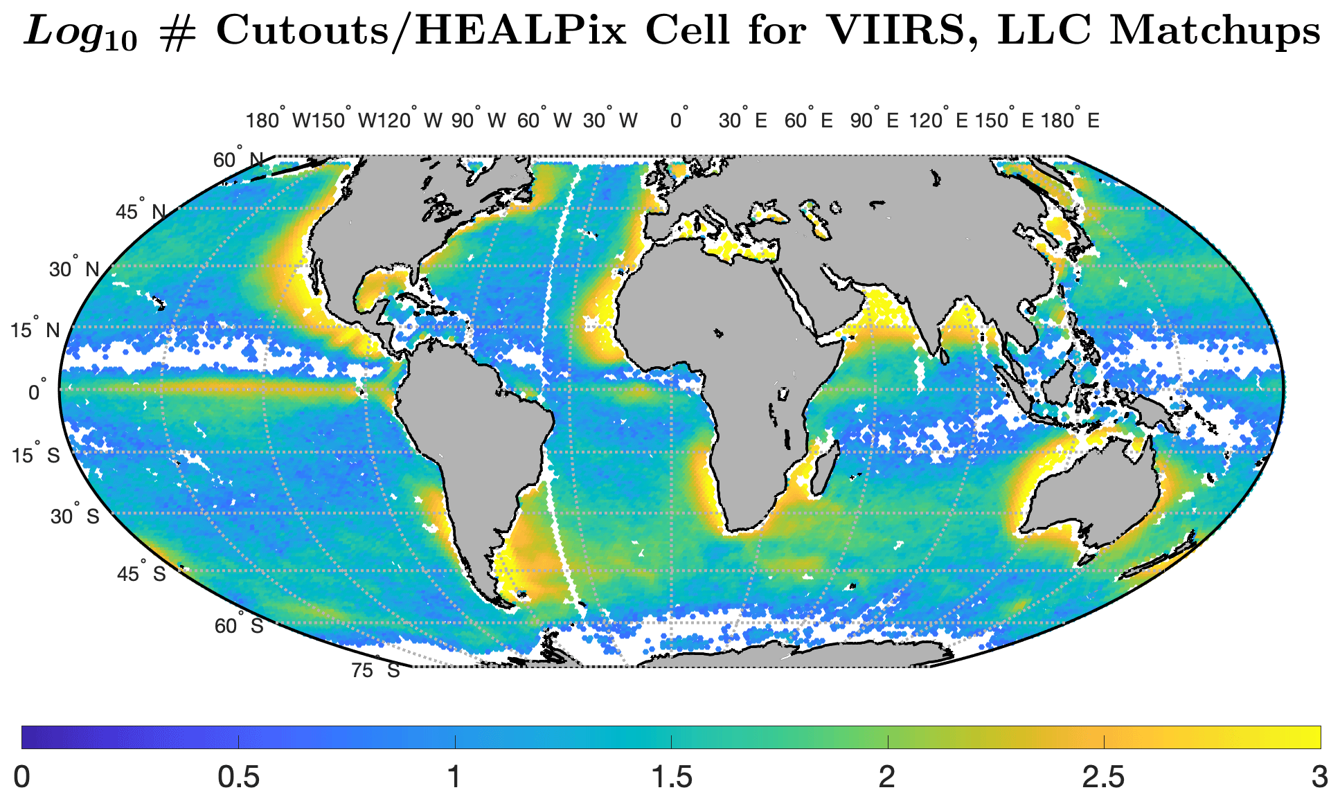
Figure 1Geographic distribution of cutouts in our 98 % clear VIIRS dataset, shown using a log10-based scale of color intensity. Each equally sized (HEALPix) spatial cell, plotted as dots here, covers approximately 10 000 km2. HEALPix cells with fewer than five VIIRS cutouts or fewer than five LLC4320 cutouts are shown in white. Land is shown as light gray. Meridional white line at ∼ 35∘ W is due to an LLC4320 sampling artifact.
For cutouts with one or more masked pixels, we “inpainted” them using the biharmonic algorithm provided in the scikit-image software package (van der Walt et al., 2014); the algorithm, we found, performs well even for data with steep gradients (Prochaska et al., 2021). We then downscaled the arrays with a local mean to 64 pixels × 64 pixels or approximately 144 km × 144 km at ∼ 2.1 km sampling, which approximately matches the coarsest sampling of the LLC4320 outputs. Note that the actual size of cutouts is a function of distance from nadir; we did not resample the observed data to account for these changes. Last, we demeaned each cutout to produce SST anomaly (SSTa) fields. This defines the final, preprocessed dataset that we use for all VIIRS analyses to follow.
3.1.2 LLC4320 cutouts
Roughly 9 years (8 years, 11 months) of VIIRS data comprise the ∼ 3 million (2 932 452) VIIRS cutouts, whereas the LLC4320 simulation output used for this study spans only 1 year. To further restrict the VIIRS cutouts to 1 year would leave too few data for a full-globe comparison between satellite observations and the model outputs. For this reason, we compare ∼ 9 years of VIIRS data to the 1-year model simulation.
Our approach to constructing cutouts from the LLC4320 outputs intentionally paralleled the methodology and outputs for VIIRS. We first identified all 64 pixel × 64 pixel regions that have a valid SST value (i.e., avoiding land). The geographic location (lat, long) of each of these was recorded. Second, we considered the full year of LLC4320 outputs taken every 12 h from 17 November 2011 to 15 November 2012 (inclusive). For each cutout in the VIIRS sample, we matched the location to the closest valid 64 pixel × 64 pixel region in the LLC4320 dataset. We then identified the LLC4320 timestamp closest in time from the start of the given year (with the LLC4320 in 12 h intervals). This is akin to matching on the day of the year and then the time of the day to the nearest 12 h. This “climatological” matchup of cutouts was performed to avoid seasonal and regional biases in the sampling.
Much of the analysis presented in subsequent sections of this paper compares the statistics of cutouts in a given HEALPix cell. Ideally, the cutouts associated with a VIIRS–LLC4320 matchup lie in the same HEALPix cell. This, however, is not always the case; the closest LLC4320 cutout to a VIIRS cutout may lie in an adjacent HEALPix cell when the VIIRS cutout lies outside of the LLC4320 grid, generally in coastal waters.
We wished to maintain an approximately constant sampling size of 2.25 km matched to VIIRS or a 144 km × 144 km total for a 64 pixel × 64 pixel cutout. Therefore, we sized the array extracted from the LLC4320 outputs according to the local size of the grid, which varies as approximately cos (lat) for latitudes N. At latitudes N, LLC4320 horizontal grid spacing asymptotes to ∼ 1 km in the polar cap. To avoid the complications brought by different grid characteristics, we constrained our analysis to an area south of 57∘ N.
Each extracted LLC4320 array is downscaled to a 64 pixel × 64 pixel cutout using the local mean. We then injected random noise using a Gaussian deviate with a standard deviation of σ=0.04 K based on an analysis of the noise properties of the VIIRS data (Wu et al., 2017). Lastly, we demeaned each cutout to generate SSTa arrays.
3.2 Characterization of the SSTa cutouts
Each cutout was assigned a log-likelihood (LL) metric by the machine learning algorithm, ULMO, used for this work. This metric describes the frequency of occurrence of the cutout within the full set. The LL metric tends to correlate with the SST structure, at least at the spatial scales of the fields under consideration here, with structure increasing with a decreasing LL (Prochaska et al., 2021). This simply follows from the fact that the parent sample is dominated by cutouts with little inherent structure. Comparing the distribution of LL values across the global ocean thus identifies geographic regions where the structure of the model output at submesoscale-to-mesoscale levels matches (or fails to match) the observations.
3.2.1 Brief overview of ULMO
The ULMO machine learning algorithm is a probabilistic autoencoder (PAE; Böhm and Seljak, 2020) designed to assign a relative probability of occurrence to each cutout in a large dataset. It is an unsupervised method which learns representations of the diversity of SSTa patterns without human assessment. The PAE combines two deep learning algorithms to perform its analysis. The first is an autoencoder that generates a reduced dimensionality representation (a.k.a., a latent vector) for each cutout in a complex latent space. The second step is a normalizing flow (Papamakarios et al., 2019) which transforms the autoencoder latent space into a Gaussian manifold with the same dimensionality. One can then calculate the relative probability of any cutout occurring within the Gaussian manifold with standard statistics. We refer to this relative probability as the log-likelihood (LL) metric.
In the following section, we compare distributions of the LL metric for the VIIRS and LLC4320 cutouts in discrete geographical regions across the global ocean. This provides a quantitative technique to compare the SSTa patterns predicted by the OGCM against those observed in the real ocean. We note that because the LL metric is only a scalar description of a given pattern's frequency of occurrence, it is possible – in principle – to have similar LL distributions despite qualitative differences in the SSTa patterns. This would, however, require a remarkable coincidence, and our visual inspection of regions with consistent LL distributions have not revealed any such examples. We also emphasize that the opposite is not true: regions with significantly different LL distributions do have qualitatively differing distributions of SSTa patterns.
Figure 2 presents galleries of VIIRS and LLC cutouts designed to show how the structure of the cutouts vary as a function of LL. For Fig. 2a, the entire LL VIIRS population is divided into quintiles. For each quintile, one VIIRS cutout and one LLC cutout is randomly selected from the 50 LL values nearest to the median of the VIIRS LL distribution. The LL of the median values are shown above the VIIRS cutouts. These galleries show a well-defined progression from fields with a large temperature range and accompanying gradients to fields with a smaller temperature range, weaker gradients, and less complex patterns.
The correlation between temperature range and LL seen in Fig. 2a was noted by Prochaska et al. (2021) in their discussion of the MODIS dataset. In the analysis to follow (Sect. 4.2), we compare LL values of VIIRS cutouts with those for LLC cutouts at the same geographic location, which suggests that the temperature range of the cutouts we compare will be similar. (Admittedly, there are a few regions where this is not the case, and we address this when it occurs.) Important from the perspective of the work presented herein is rather how the characteristics of cutouts vary with LL when the temperature range is bound to a small range. To further provide a sense for how cutout characteristics other than temperature range evolve with LL, we present a second gallery of VIIRS and LLC cutouts in Fig. 2b. These cutouts are restricted to have K, where ΔT is defined as the difference in 90th and 10th percentiles of the SST distribution: , where TN denotes the Nth percentile. These galleries were constructed in the same fashion as those for Fig. 2a. In this case, the progression is from cutouts for which SST contours are relatively convoluted to cutouts with relatively straighter contours; in other words, the “structure” of the cutouts decreases as LL increases. As with the galleries in Fig. 2a, the characteristics of the LLC cutouts in this gallery track those of the cutouts in the VIIRS gallery.
As noted above, the galleries of Fig. 2 show how the structure of the cutouts varies with LL. However, they do not relate the LL to the underlying dynamics, which would be helpful in obtaining a better understanding of regions in which the LLC appears to fail. We are working on trying to establish such a relationship, if one exists, but to date, it eludes us. The lack of such a relationship, however, does not invalidate the results of this work in that whatever the relationship, it applies equally to VIIRS and LLC4320.
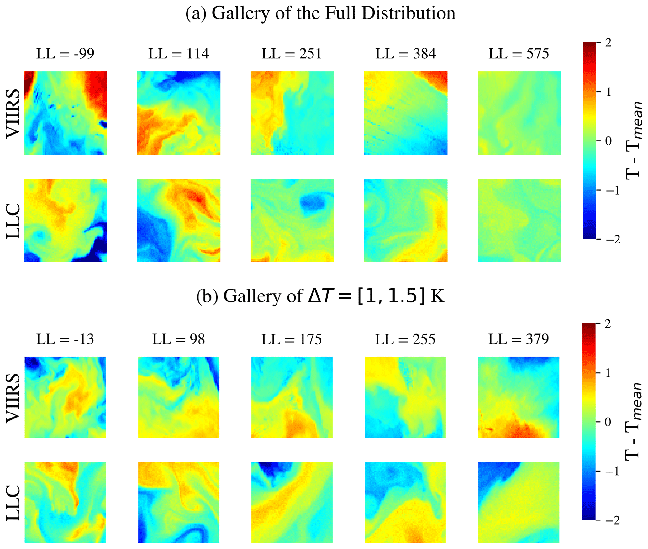
Figure 2 Galleries of cutouts showing the progression of the structure of the associated SST fields as a function of LL. (a) Galleries for the entire set of cutouts. Upper row is for VIIRS cutouts; lower row is for LLC cutouts. Each cutout is randomly selected from the 50 cutouts with the LL nearest to the median VIIRS LL value for the associated LL quintile. The LL of the median is shown above the VIIRS cutout. (b) Similar galleries for all cutouts with K, where with TN denoting the Nth percentile.
3.2.2 Training on VIIRS and evaluation
In Prochaska et al. (2021) we introduced the ULMO algorithm and trained a model with Level-2 (L2) MODIS data sampled at ∼ 2 km and using 64 pixel × 64 pixel cutouts. While this model could have been applied here to the VIIRS and LLC4320 cutouts, we have generated a new ULMO model from the VIIRS dataset. The same hyperparameters derived for ULMO in Prochaska et al. (2021) were adopted here.
We trained the PAE on 150 000 random VIIRS cutouts from 2013 and used the remainder of the data from that year (181 184 cutouts) for evaluation. We trained the autoencoder for 10 epochs with a batch size of 256 and achieved good learning loss convergence. We then trained the normalizing flow for 10 epochs (batch size of 64) and also achieved good convergence. The VIIRS-trained ULMO model was then applied to all of the VIIRS and LLC4320 cutouts to calculate LL for each.
We divide the comparison of the VIIRS SST dataset with the LLC4320 model output, in the context of the patterns learned by ULMO, into those related to the shapes of the two LL probability distributions and those related to their geographic distributions.
4.1 Overall statistical comparison of VIIRS and LLC4320 LL values
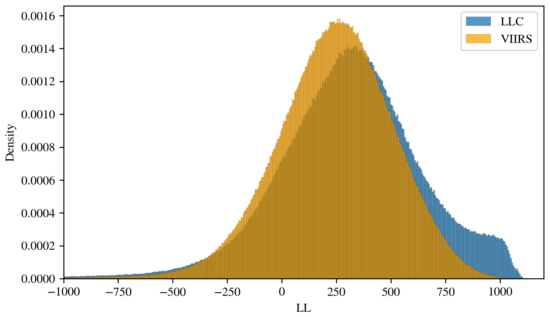
Figure 3 compares the distribution of the LL metric for the 9 years of VIIRS observations against the LLC4320 results matched in space and according to the day of the year. The two distributions are quite similar, suggesting that, on average, the SST pattern distribution learned by ULMO from VIIRS is close to the same distribution derived from LLC4320. There are, however, differences, subtle for much of the range of LL values and not so subtle for LL>800.
-
The range corresponds to relatively energetic regions, generally associated with strong currents and large SST gradients (Prochaska et al., 2021). In these regions, the probability of finding a VIIRS cutout with a given LL value is lower than that of finding an LLC4320 cutout with the same LL value. This suggests that in dynamic regions, LLC4320 fields tend to have slightly more structure than VIIRS fields, i.e., that the fields are possibly more energetic. An example of cutouts in this LL range is discussed in the paragraphs following the bolded text of Gulf Stream in Sect. 4.2.2.
-
The range corresponds to mid-range fields, generally found at mid-latitudes (Fig. 4a), away from eastern and western boundary currents. The probability of finding a VIIRS cutout with a given structure (LL value) in this LL range is increasingly higher, as LL increases from −375 to 375, than that of finding an LLC4320 cutout within this LL range. An example of cutouts in this LL range is discussed in the paragraphs following the bolded text of Southern Ocean in Sect. 4.2.2.
-
In the range, the probability for the LLC4320 of finding a given LL value is higher – less structure – than for VIIRS. SST fields with these LL values have relatively little structure with retrieval and instrument noise associated with the satellite-derived fields having a relatively larger impact on their observed structure. As noted in Sect. 3.1.2, white noise was added to the LLC4320 fields in an attempt to remove the importance of noise in determining the LL value, but, in retrospect, the level of noise may not have been sufficient to address this, hence the higher probability of finding LLC4320 cutouts in this range. Cutouts of LL>375 tend to be found equatorward of approximately 15∘.
-
For the LL>800 range, the probability distribution for LLC4320 LL values levels off at 800, falling rapidly to 0 for values larger than 1100 or so. By contrast, few VIIRS cutouts have LL values greater than 800. This is likely due to noise in the satellite-derived SST cutouts as well as unresolved clouds, discussed in the paragraphs following the bolded text of Equatorial band in Sect. 4.2.2.
4.2 Geographic comparison of and values
As mentioned in Sect. 3.1.1, we compare the geographic distribution of VIIRS LLs with that of LLC4320, based on the HEALPix-tesselated surface covering the entire Earth: 41 952 equal-area spatial cells, each of ∼ 100 km × 100 km size. Within each cell, we consider the distribution of LL values from the VIIRS data and LLC4320 output. To minimize the effects of outliers within the distributions, we utilize the median LL value (designated hereinafter) as a characteristic metric of the structure in SST at a given location. Furthermore, we only consider HEALPix cells containing at least five VIIRS cutouts and five LLC4320 cutouts. The distributions for and are shown in Fig. 4 and their difference, ΔLL=, in Fig. 5. Recall that LL tends to increase with decreasing structure in the SSTa field; hence positive values of ΔLL suggest less structure in the satellite-derived cutouts than in the cutouts of the model output, and negative values suggest the contrary.
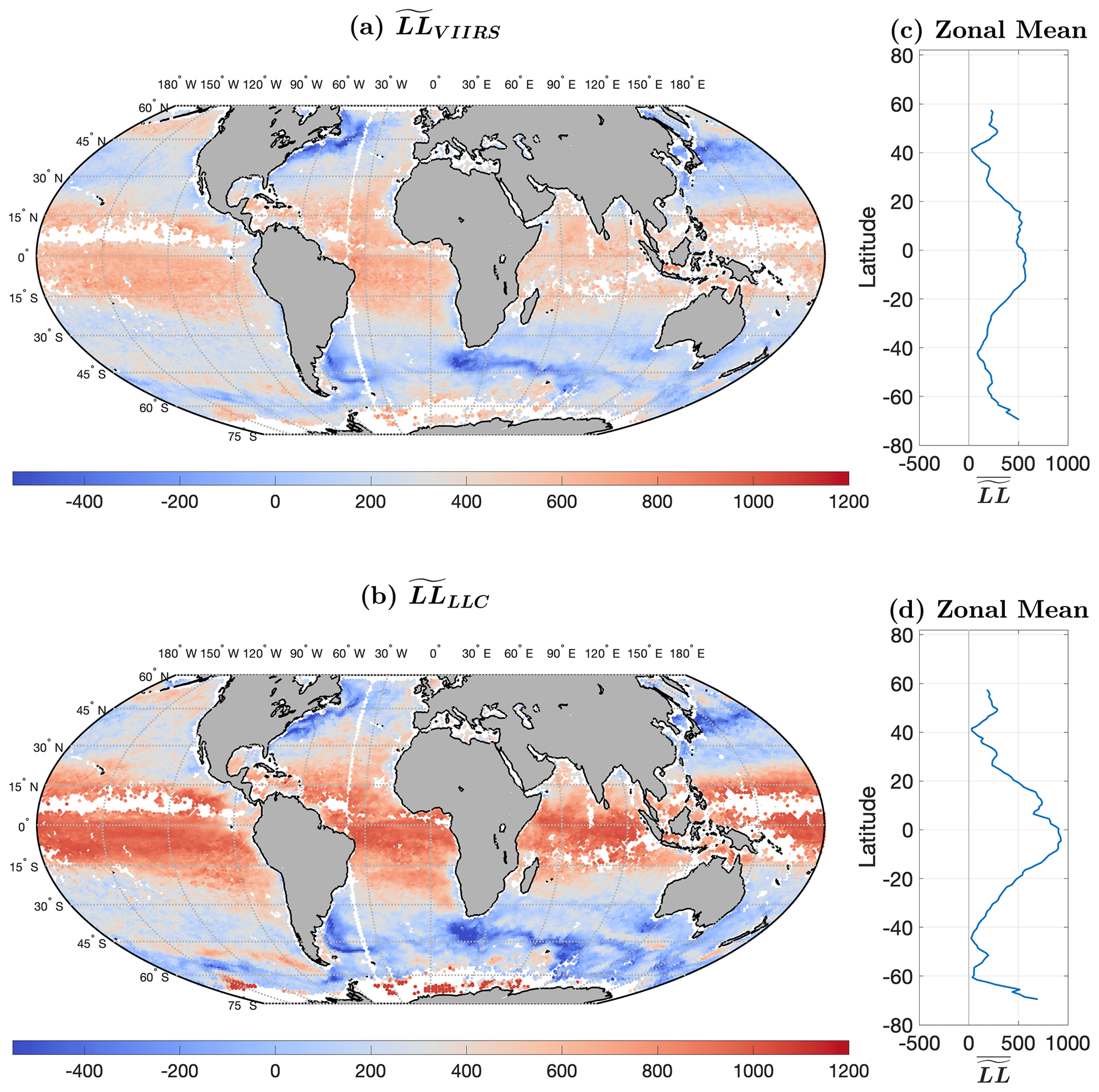
Figure 4HEALPix median LL for (a) VIIRS cutouts (), (b) , (c) the zonal average of , and (d) the zonal average of . Each dot in (a) and (b) is associated with an equal-area HEALPix cell. White dots correspond to locations with fewer than five VIIRS cutouts and fewer than five LLC4320 cutouts in the HEALPix cell. Land is shown in gray.
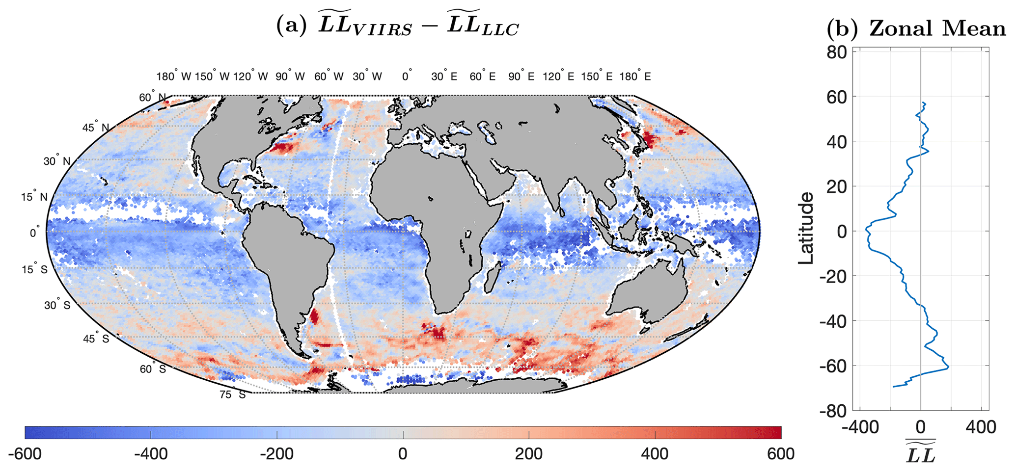
Figure 5(a) . (b) Zonal mean of . It is apparent that the LLC4320 model has SST patterns with less structure in equatorial regions. In contrast, the dynamic regions of the global ocean (e.g., western boundary currents) exhibit lower , indicating a higher degree of structure within these areas in the model output.
Figure 5 suggests that there are significant differences between the submesoscale-to-mesoscale structure of the simulation and that of the satellite-derived dataset. However, closer examination of the two plots in Fig. 4 suggests that there is significant similarity in the larger scale (more than several hundred kilometers) of the two fields; our eyes are drawn to the differences, the large red equatorial regions and blue regions at higher latitudes, not the similarities. We therefore begin by examining the similarities of the fields and then consider their differences.
4.2.1 Similarities
To highlight the similarities in the fields on smaller scales (𝒪(100 km)), we remove the large regional differences from apparent between them (Fig. 4). This is done by averaging and over 100 sequential values based on the HEALPix index. HEALPix cells are arranged longitudinally, so this correction removes zonal structures on the order of 10 000 km or longer, retaining structures on smaller spatial scales. (black) and (cyan) are shown in Fig. 6. A “corrected” , designated as , is then determined from
where i∈ all HEALPix cells with at least five cutouts in the VIIRS dataset and five cutouts in the LLC4320 dataset of
and ⌊x⌋ denotes the largest integer less than or equal to x. values are shown in red in Fig. 6.
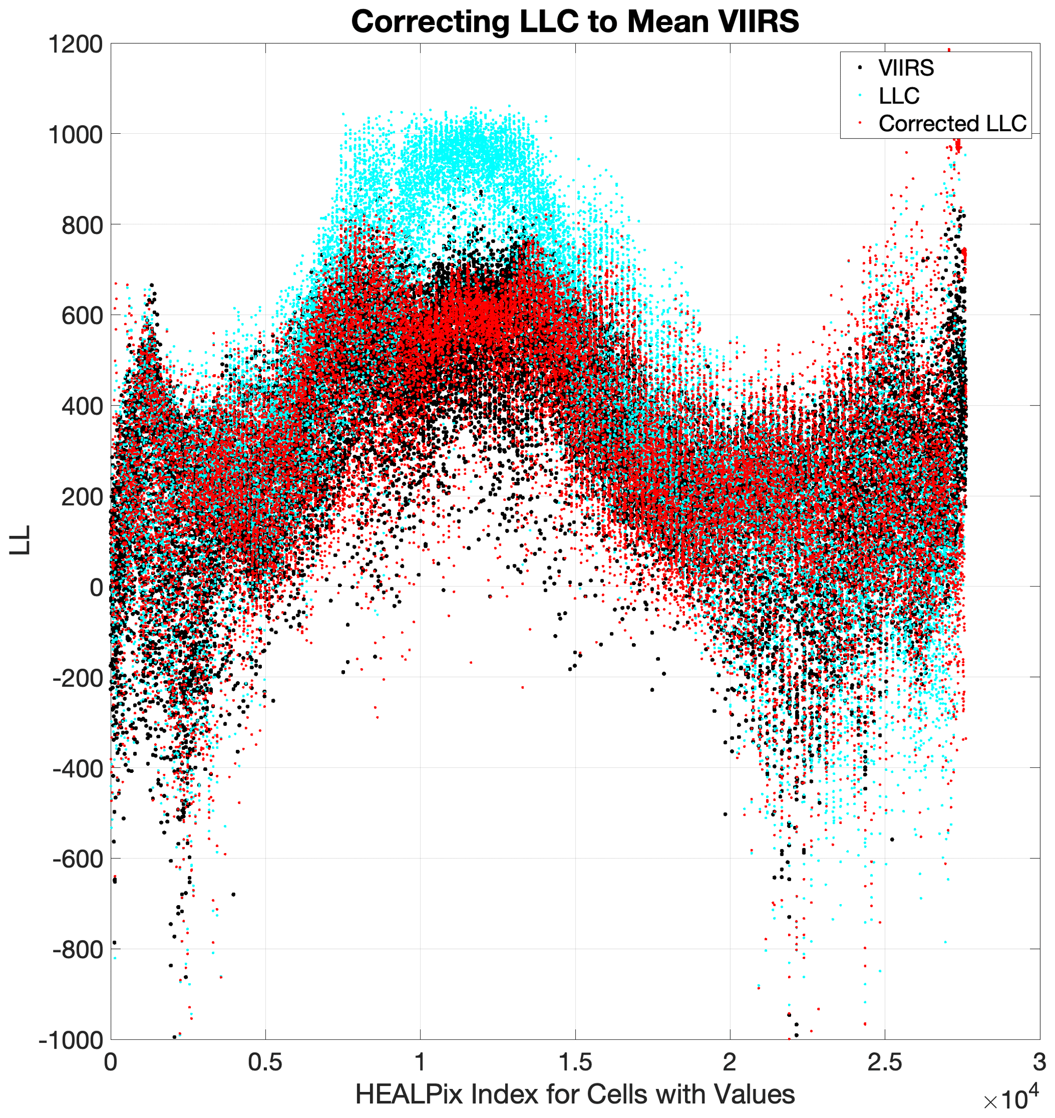
Figure 6 versus HEALPix cell index: values are black dots, values are cyan, and values are red.
The plots, in Fig. 7, bin each HEALPix cell by their associated values. The left histogram bins the cells according to their and values, whereas the right histogram bins according to their and values. As noted in Fig. 3, cutouts in the LLC dataset skew to higher LL values than those found in the VIIRS dataset. The difference in the LL distributions can also be seen in Fig. 7a, where values, greater than approximately 200, tend to be higher than values with the separation increasing with LL. It is important to note that here we have binned the HEALPix cells and their values, not the cutouts and their LL values. Correcting the values lowered the values to be more in line with the values.
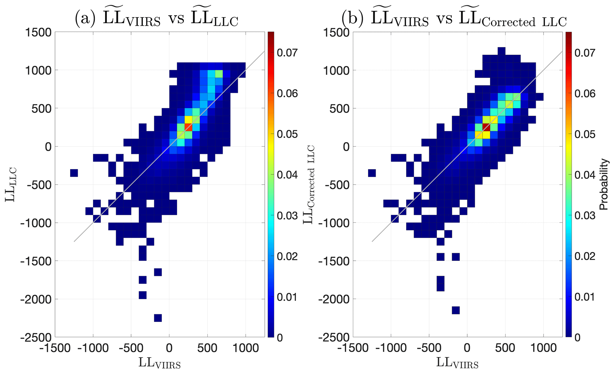
Figure 7 and values of each HEALPix cell are plotted in a 2-dimensional histogram on the left, whereas the right 2-dimensional histogram bins cells according to their and values. The same color bar is used for both histograms; colors range from blue (a lower cell count) to red (a higher cell count).
The geographic distribution is shown with that of in Fig. 8. The large-scale similarities in the general shape of the distributions is much more evident in this figure, but of more interest are the many smaller-scale features, which emerge in the corrected distribution. Consider, for example, the fields at approximately 45∘ S in the black and red polygons of Fig. 9. For both and there is a local maximum in corresponding to a minimum in the structure of the SSTa cutouts in the black polygon. This feature is associated with a zonal bathymetric ridge at approximately 45∘ S crossed by two meridional ridges, one at W and the other at W (Fig. 10b, although the ridges are difficult to see in this figure). The peaks of these ridges are at depths of approximately 5000 m in a basin extending to depths of 6000 m. Both fields show a band of negative values to the west and south of the feature. The field also shows a well-defined band to the north and east, while the fields only shows a suggestion of such a band, but the local minimum is still well defined in both.
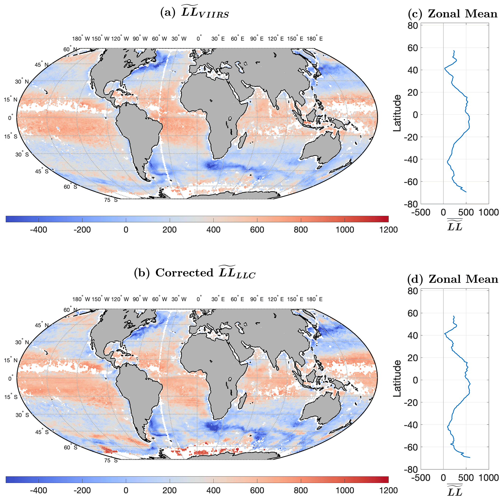
Figure 8As in Fig. 4 except is shown in (b).
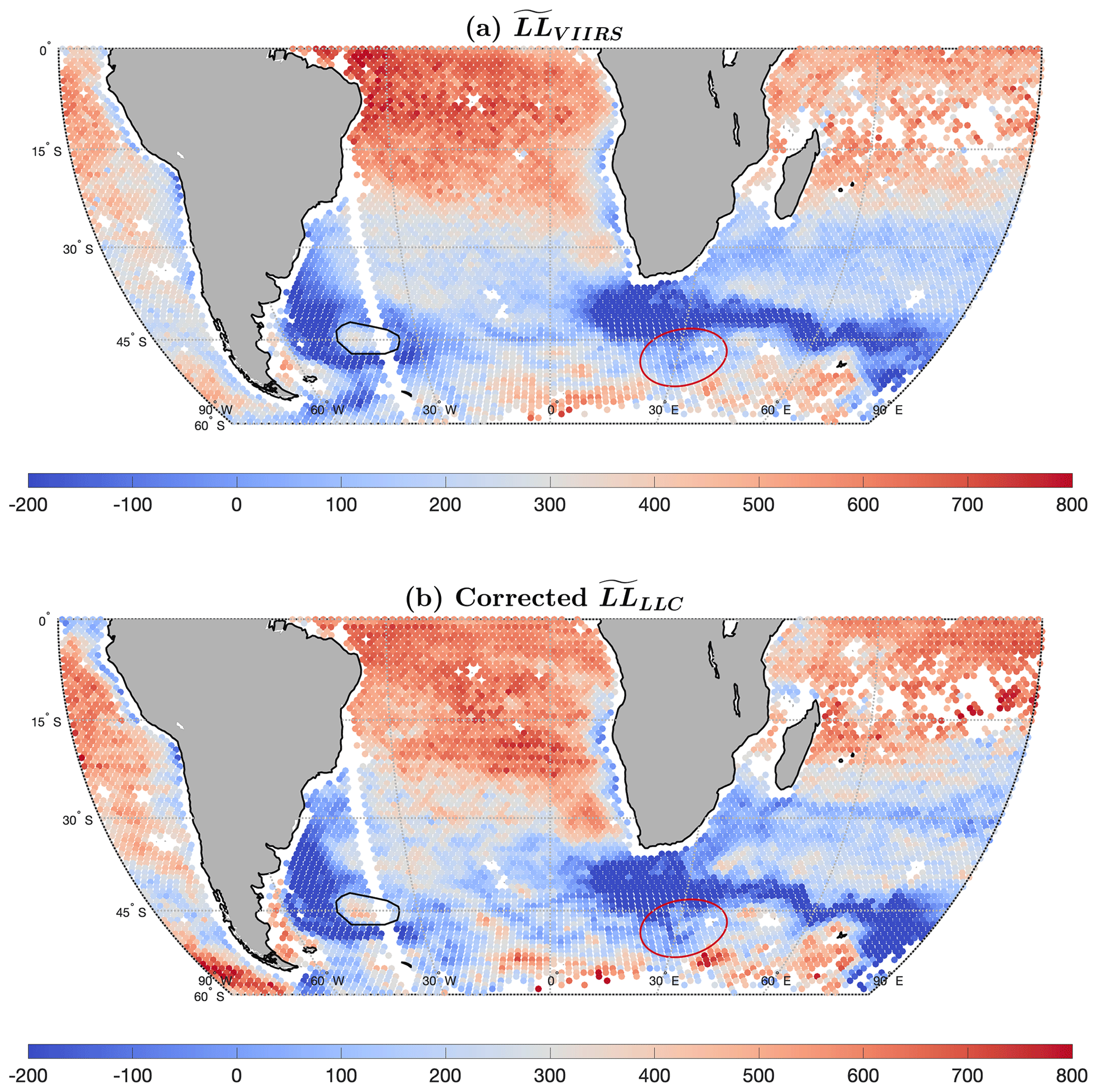
Figure 9As in Fig. 8 but with a palette constrained to better show features in the two focus area: black polygon at ∼ 35∘ W, 45∘ S and red polygon at ∼ 30∘ E, 50∘ S.
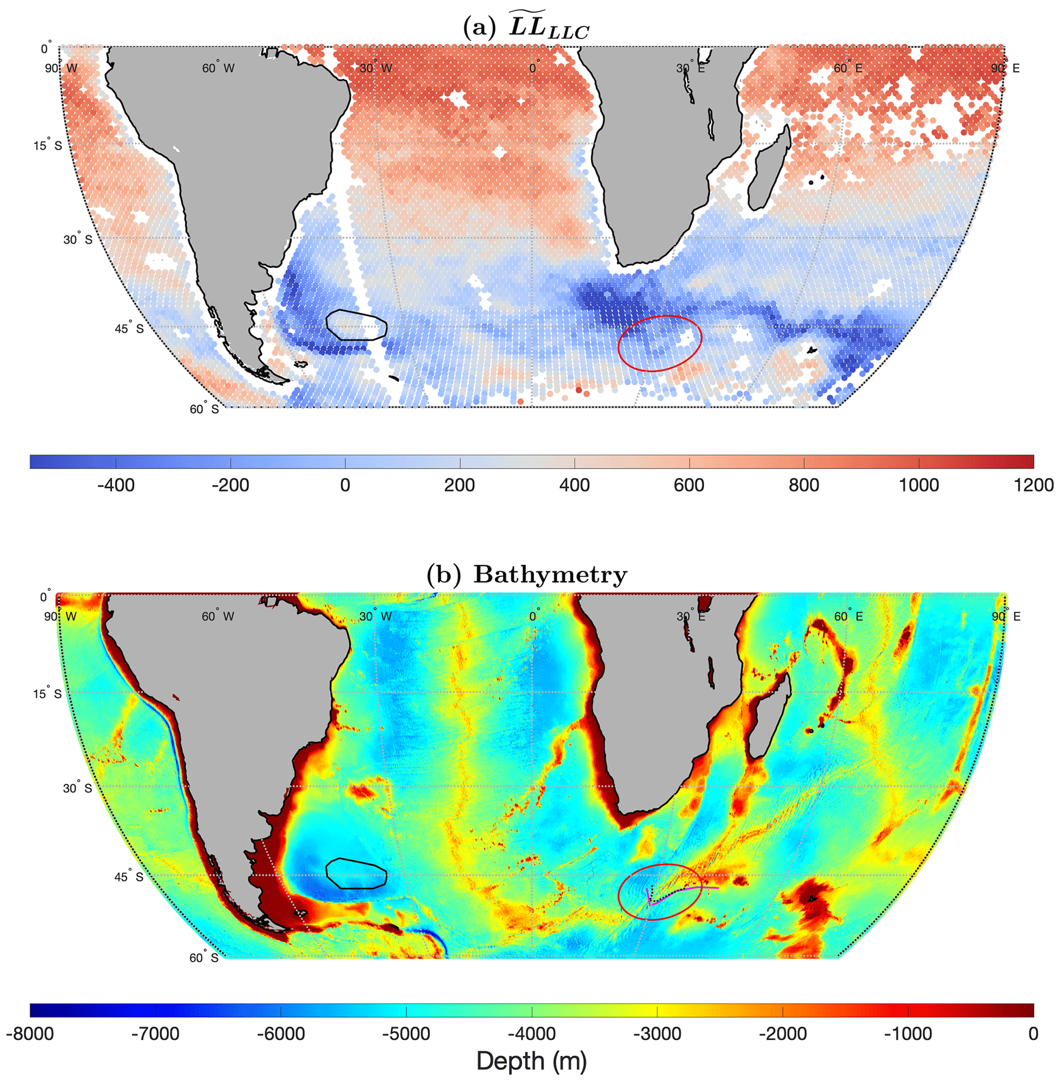
The second feature of interest is the thin, hooked band of low values – corresponding to relatively more structure in the cutouts – in the red polygon south of South Africa (Fig. 9a). This band is reproduced well in the LLC4320 output (Fig. 9b). Again, referring to the bathymetric image (Fig. 10b), it is clear that the shape of this feature is a consequence of the underlying bathymetry. Specifically, it appears that a tendril of the retroflected Agulhas Current has flowed to the south before turning toward the east to pass through a gap in the southwest–northeast ridge, partially blocking the main part of the retroflected current. The top of the ridge is found at depths of approximately 2000 m, while the relatively wide gap, through which the tendril passes, is as deep as 3500 m. The manually digitized center of the feature is shown with the dotted black and solid magenta lines in Fig. 10b; the model appears to reproduce this subtle feature in the circulation quite accurately.
4.2.2 Differences
To highlight the regional distributions with significant differences between the structure of satellite-derived and LLC4320-produced SSTa cutouts, we replot the data of Fig. 5 in Fig. 11 but mask all values between −197 and 197 in dark gray. These thresholds determine what ΔLL values we consider to be statistically significant; they are the differences in the LL distributions from the first 4 years, 2012–2015, to the last 4 years, 2017–2020, of VIIRS data. Any differences within those given thresholds can be attributed to statistical variability between the simulation of a free-running model and observational data. HEALPix cells with ΔLL values beyond these thresholds correspond to regions either for which the retrieved VIIRS cutouts are not good measures of SST or for which the LLC4320 output is associated with deficiencies in the simulation (see Appendix A for more detail).
differences evident in Fig. 11 fall into three general groupings: the wide band of negative values (more structure in the VIIRS cutouts than in the LLC4320 cutouts) centered on the Equator; the less continuous band of positive values in the Southern Ocean; and the very positive (much more LLC4320 structure than VIIRS structure) patches in the vicinity of the separation of western boundary currents from the continental margin, specifically, the Gulf Stream in the western North Atlantic, the Kuroshio in the western North Pacific, the Brazil Current in the South Atlantic, and the Agulhas Current where it retroflects south of South Africa. The equatorial and Southern Ocean bands are also evident in the zonal mean of of the unmasked field shown in Fig. 5b. The zonal mean is roughly flat at −350 from 5∘ S to the Equator; rises rapidly poleward of these two points for about 5∘ of latitude to −150; and then continues to increase approximately linearly but, more slowly, from there (10∘ S and 5∘ N) to a value of 0 at 30∘ N and 30∘ S.
In the text to follow, we address each of the three regions primarily in the context of SST galleries constructed from two small and geographically close regions (three colored rectangles shown in Fig. 11), which exemplify characteristics of the differences that we find to be of interest.
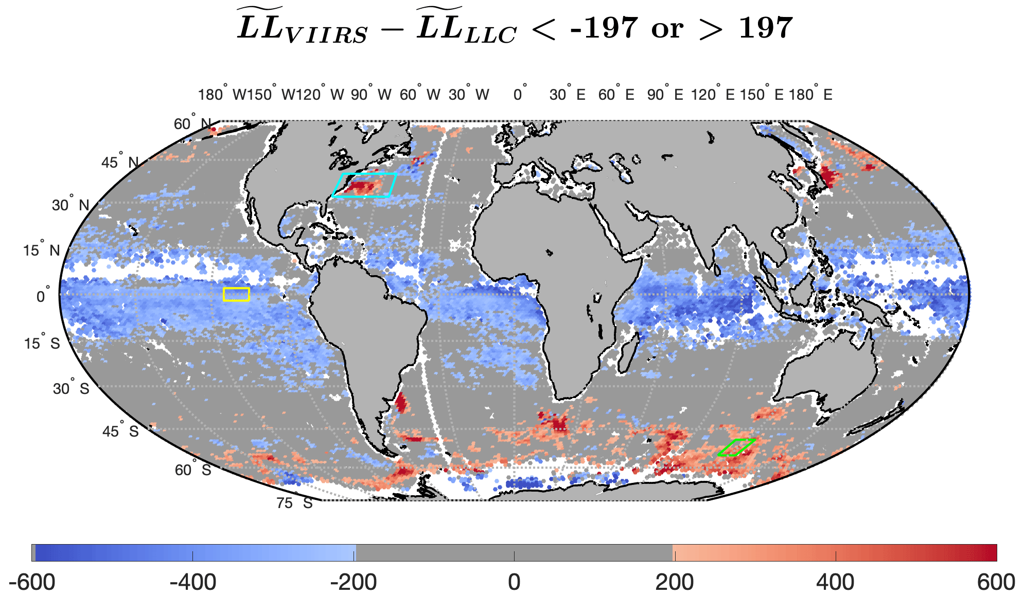
Figure 11As in Fig. 5a with masked darker gray to highlight the significant differences between VIIRS observations and the LLC4320 model outputs. The yellow rectangle (∼ 110∘ W, 0∘ N) designates the focus area for galleries shown in Fig. 14, highlighting equatorial differences; the green rectangle (∼ 120∘ E, 55∘ S) designates the focus area for galleries shown in Fig. 16, highlighting Southern Ocean differences; and the cyan rectangle (∼ 70∘ W, 35∘ N) designates the focus area for galleries shown in Fig. 18, highlighting western boundary current differences.
Equatorial band
In general, there are four possibilities for low values of in the equatorial region (15∘ S to 15∘ N).
-
The year simulated, 2012, is atypical, differing from the 2012–2020 mean. This is very unlikely given the magnitude of the differences, −350 at the Equator, as well as the fact that the zonal mean of is essentially flat at 0 equatorward of 50∘ (Fig. A3), suggesting little interannual variability.
-
Unresolved clouds exist in the VIIRS cutouts. Unresolved clouds tend to add structure to the cutouts; the “quieter” the field is, the more significant the impact noise is on the structure and the greater the decrease will be in . To address this potential problem, the 194 cutouts of the HEALPix cell at 36∘ N, W were examined for unresolved clouds. Thirty percent were found to be of high quality, 50 % were found to be significantly contaminated, and there was uncertainty as to how to classify the remaining 20 %. Calculating mean for the high-quality-only cutouts increased the mean value by 43, which is small compared to the difference of −350 for this HEALPix cell, so this is not likely the primary explanation for the differences. We further address this issue below in the context of galleries of SST fields.
-
Noise exists in the VIIRS SST fields. Cutouts in this part of the ocean tend to have relatively high values (Fig. 4a), corresponding to relatively less structure. This means that noise in the field, which is assumed to change slowly if at all with latitude, will become relatively more important, decreasing . Noise has been added to the LLC4320 SST fields in an attempt to address this, but it is possibly not enough, resulting in more negative values of .
-
LLC4320 does not reproduce the submesoscale-to-mesoscale structure well in the equatorial regions. There is a suggestion based on the examination of a small patch of this region, discussed below, that the model is missing structure in at least some parts of this region.
The rectangular patch [2∘ S–2∘ N, 105–95∘ W] west of the Galapagos Islands in the equatorial Pacific (the yellow rectangle in Figs. 11 and 12) stands out because of the significant step of along the Equator. The distribution for the region in the rectangle above the Equator is provided in Fig. 13a, as well as below the Equator in Fig. 13c. Consistent with the geographic distributions of in Fig. 4, the median value increases from south to north across the Equator, while the median value decreases, both contributing to a larger structural difference between VIIRS cutouts and LLC4320 cutouts to the north of the Equator than that to the south. Histograms of ΔT are provided because there is a correlation, although weak, between LL and ΔT, while ΔT is a more readily understood measure of similarity and differences between VIIRS and LLC4320 SST fields. The distribution of ΔTLLC is similar across the Equator, while that of VIIRS shows a much longer tail consistent with more variability and lower LL values.
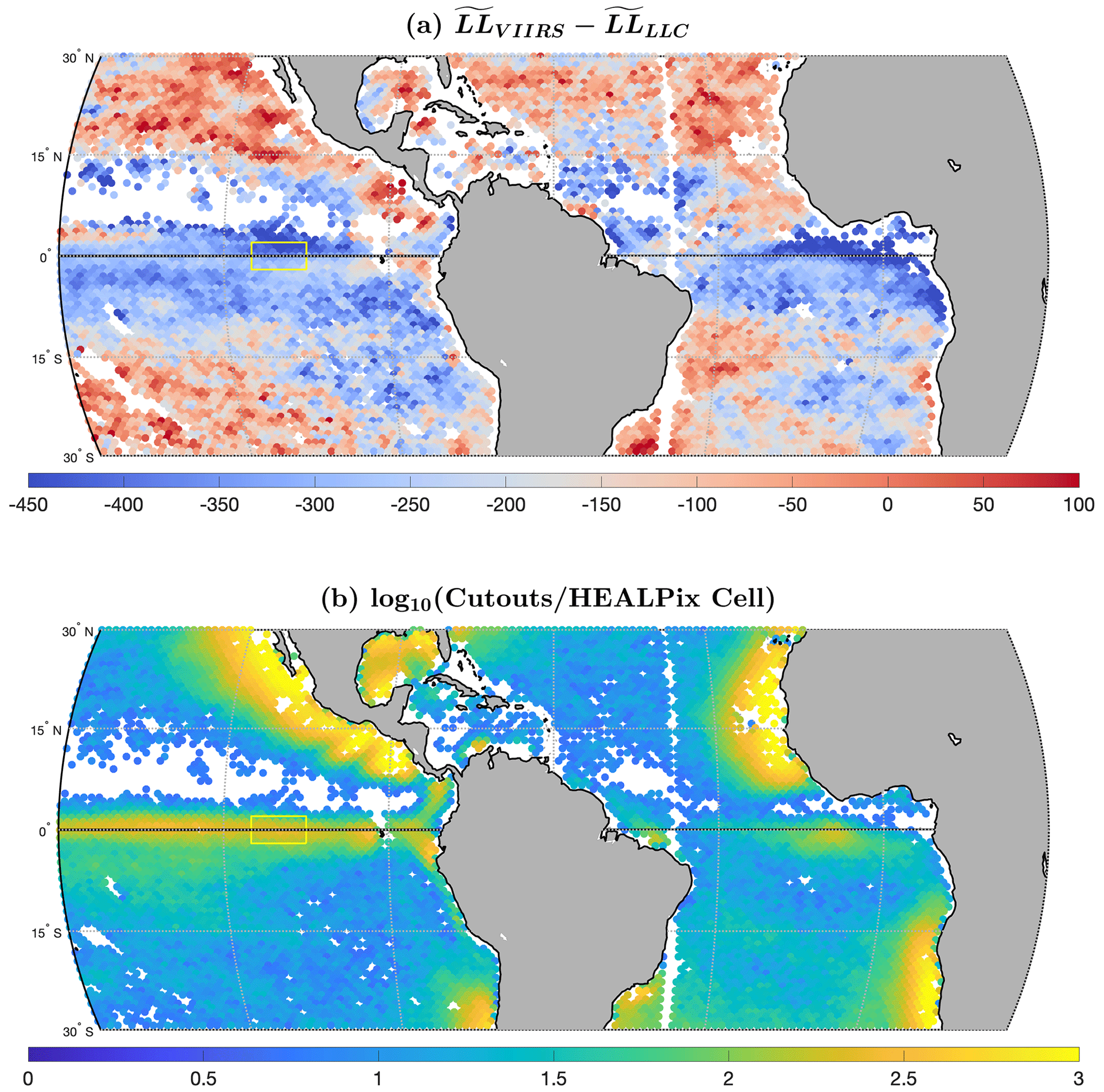
Figure 12(a) for the equatorial Pacific and Atlantic. (b) The log 10 of the number of cutouts per HEALPix cell. Thick horizontal black line is the Equator. Yellow rectangle is the focus area.
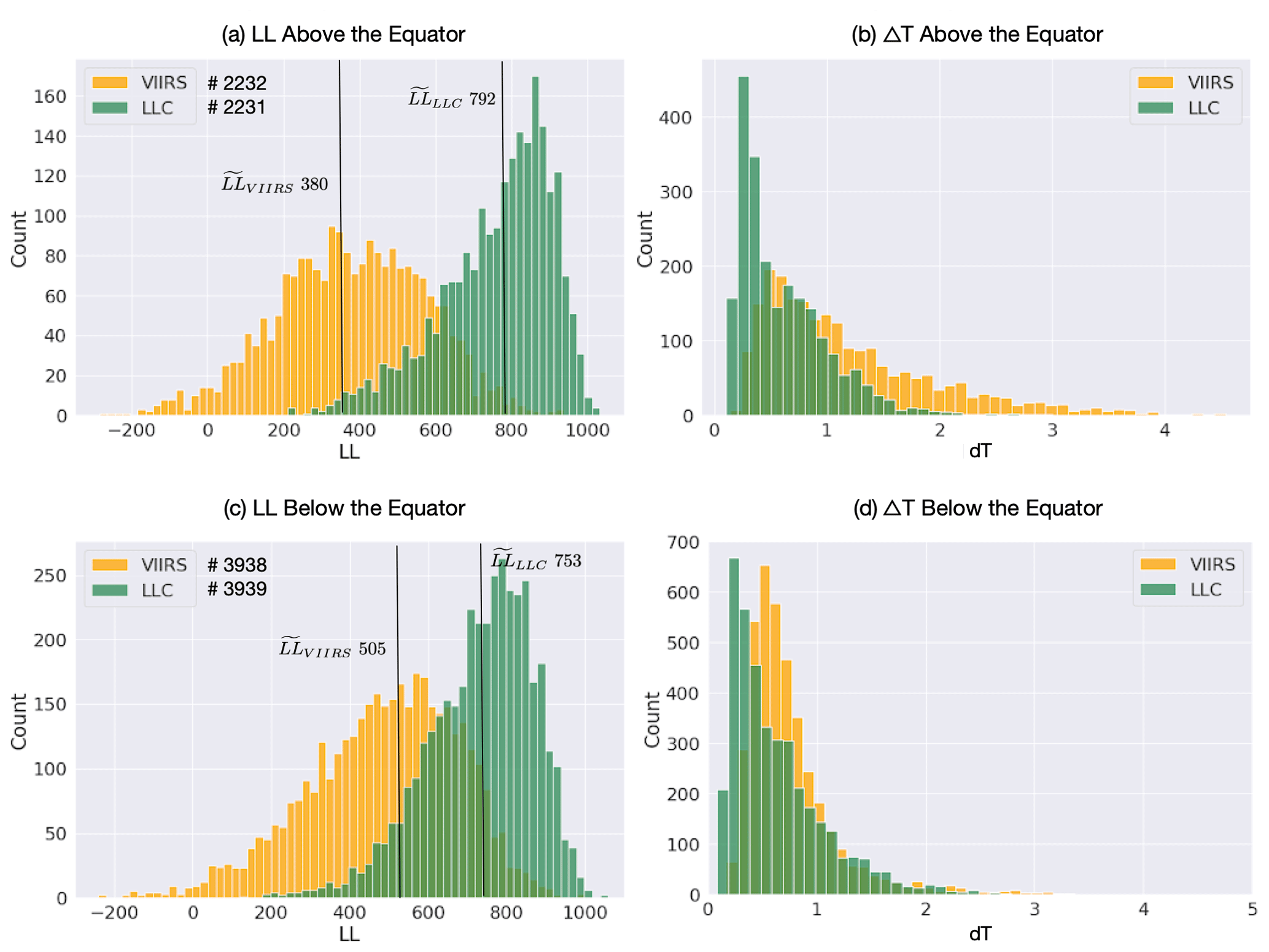
Figure 13(a) Histograms of LL for all VIIRS (yellow) and LLC4320 (green) cutouts above the Equator in the focus area. (b) Histograms of ΔT for the same region as (a). (c) As for (a) except below the Equator. (d) As for (b) except below the Equator. The median values of the distributions are indicated for (a) and (c), as are the number of cutouts contributing to each. The number of cutouts apply to the corresponding ΔT frames.
Visual examination of the SST fields supports the above conclusions. Consider SST fields of the VIIRS and LLC4320 cutouts in the yellow rectangle of Fig. 12, again separating them into those above the Equator and those below. Galleries of nine cutouts each are shown in Fig. 14. As previously noted each VIIRS cutout was matched in space and according to the day of the year with an LLC4320 cutout. To generate the galleries shown in Fig. 14, two sets of cutout pairs were formed. One set consisted of 40 % of all pairs in the region for which the VIIRS LL values were closest to the median VIIRS LL value for the region. The second set was similarly constructed, except being based on LLC4320 LL values. The intersection of the two sets defined the pool from which nine cutout pairs were randomly drawn. These pairs for the region above the Equator, 0 to 2∘ N and 105 to 95∘ W, are shown in Fig. 14a and b. For each VIIRS cutout in Fig. 14a, its LLC4320 partner is shown in the same location in Fig. 14b. Similarly, Fig. 14c and d show pairs for the region below the Equator. (Remember that because the LLC4320 simulation is free running, there is no reason to expect the features in the pairs to be identical or even similar; it is the structure of the fields that is of interest.) Visually, the SST fields of the LLC4320 cutouts are very similar in both regions, showing very little structure with correspondingly large LL values. The VIIRS fields below the Equator show a little more structure than the LLC4320 fields, consistent with the smaller LL values. By contrast, most of the VIIRS fields above the Equator have significantly more structure than any of those in the other three galleries, with correspondingly lower LL values. Also evident in the VIIRS galleries are blemishes in the fields, scattered regions of colder temperatures. We believe these to be unresolved clouds, i.e., clouds not detected by the retrieval algorithm. Because they add structure to the fields, we believe that they decrease the LL value of the cutout. This would reduce the magnitude of both above and below the Equator but is not likely to significantly impact the observed . Also, note that the distribution of the number of cutouts per HEALPix cell is symmetric about the Equator in the area of interest (Fig. 12b), suggesting that the contribution of clouds to corruption of the LL values is also symmetric about the Equator in the rectangle of interest.
Another possible explanation for the lack of SST structure in the equatorial region is the limited spatiotemporal resolution of the prescribed atmospheric forcing (0.14∘ and 6-hourly). A recently completed coupled ocean–atmosphere simulation (Torres et al., 2022; Light et al., 2022; Dushaw and Menemenlis, 2023) provides high-frequency/wavenumber interactive forcing (0.0625∘ and 45 s) to the ocean. We intend to repeat the present analysis on this simulation to determine whether the equatorial SST structures of this coupled simulation are more similar to VIIRS.
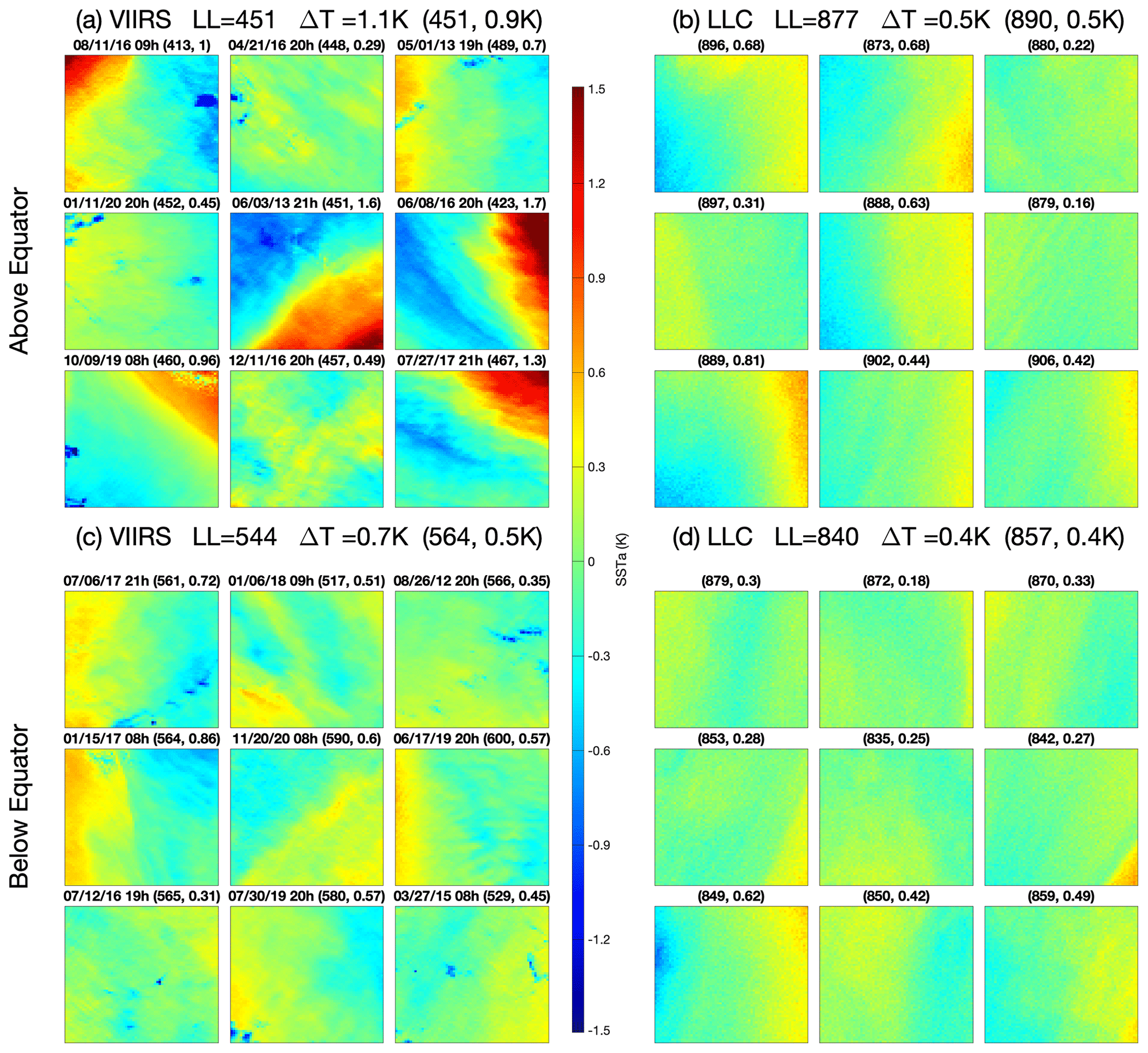
Figure 14(a) Gallery for VIIRS cutouts above the Equator in the yellow rectangle of Fig. 12a. (b) As in (a) but for LLC4320 cutouts. (c) VIIRS cutouts below the Equator in the yellow rectangle of Fig. 12a. (d) As in (c) but for LLC4320 cutouts. The mean and ΔT for all cutouts in the given region (e.g., 0–2∘ N, 105–95∘ W for a) follow the dataset name and the numbers following in parentheses are the mean and ΔT of the cutouts in the gallery. The date (month/day/year) and time of each VIIRS cutout is shown above it, and and ΔT for that cutout follow in parentheses. The date of the corresponding LLC4320 cutout (same position in the LLC4320 gallery) is the same as that of the VIIRS cutout. The time is the closest of 00:00 and 12:00 GMT to the VIIRS time. It is evident that the gallery from the VIIRS observations above the Equator shows greater structure than any of the other subsets.
Southern Ocean
We examine the same four possibilities for high values in the Southern Ocean as we did for low values in the equatorial region.
-
The year simulated, 2012, is atypical, differing from the 2012–2020 mean. This is possible but unlikely given the extent of the region covered by anomalously high differences and that there were few differences in this region for which exceeded the 2σ threshold.
-
Unresolved clouds exist in the VIIRS fields. This is very unlikely because clouds in the VIIRS fields would tend to increase the structure, which would decrease . Hence would become more positive than if clouds are not present in the VIIRS fields, rendering the difference more anomalous, not less so.
-
Noise exists in the VIIRS SST fields. This is unlikely because the geophysical variability in SST in these regions tends to overwhelm noise in the VIIRS cutouts. Furthermore, noise in the VIIRS cutouts would tend to reduce the associated , rendering the differences between uncontaminated VIIRS values and those obtained from the LLC4320 simulation even larger.
-
LLC4320 does not reproduce the submesoscale-to-mesoscale structure well in the Southern Ocean. There is a suggestion based on the examination of small patches of this region, which we discuss in more detail below, that the model has more structure in this region than is recorded in actual observations. This indicates that the mixed layer or energy dissipation and stirring due to subgrid-scale physics are not represented with sufficient accuracy in these regions.
In Fig. 15c, we replot the masked field of Fig. 10 for the Southern Ocean south of Australia with and for the same region in the upper two panels. The band of low and values from 45 to 70∘ E at about 41∘ S corresponds to the significant structure in the field associated with the Antarctic Circumpolar Current (ACC). (Note that this band originates south of South Africa where the Agulhas retroflection joins the ACC, the band of negative values of in Fig. 9.) It appears that the ACC as modeled by LLC4320 for 2012 is slightly to the south of the VIIRS ACC for 2012–2020, with the positive values of south of the band and the corresponding negative values to the north of the band. Although a small shift, the fact that the width of the bands for both VIIRS and LLC4320 is virtually identical suggests that the modeled ACC is a bit to the south of the envelope of paths in this period; i.e., the slight shift may be significant in the context of the modeled processes. Apart from the slight shift to the south, the model appears to have reproduced the current quite well in this region. East of about 70∘ E for the modeled ACC is substantially more negative than that of the observed values, resulting in the anomalous values in this region. Interestingly, east of about 95∘ E, the VIIRS field shows a positive band north and south of the northern branch of the current, as does the LLC4320 field. In fact, the general pattern of has the same general shape as that of . Therefore it appears that the model has the correct general structure for the flow in this region but, as we now emphasize, is too energetic.
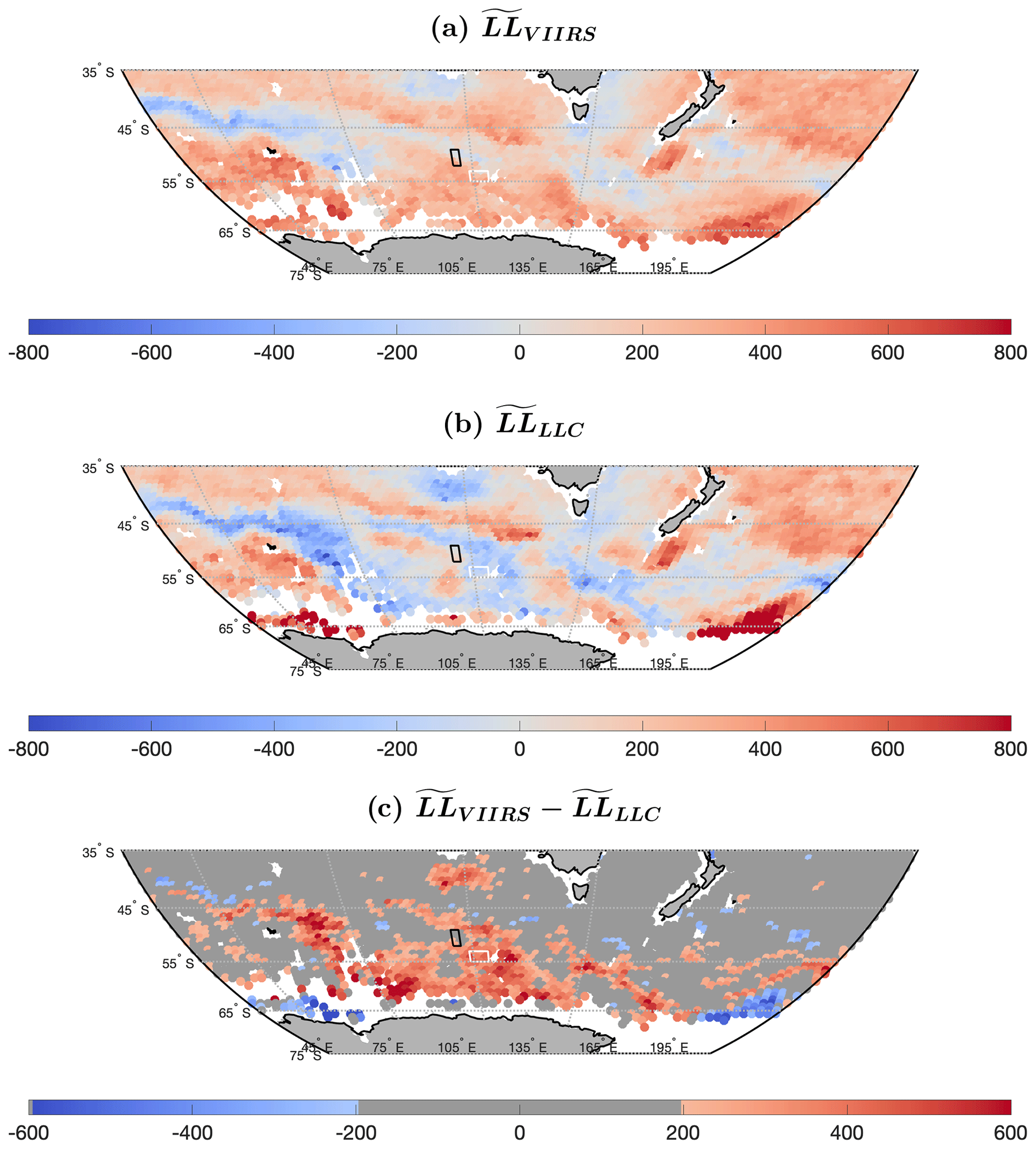
Figure 15For the focus area of the Southern Ocean, (a) , (b) , and (c) masked . The black rectangle (∼ 116∘ E, 50∘ S) indicates a region of agreement, . The white rectangle (∼ 120∘ E, 54∘ S) is an anomalous region with .
Galleries of SSTa cutouts in the black rectangles of Fig. 15 (a region for which the model values are in general agreement with the VIIRS values) are shown in Fig. 16a for VIIRS and 16b for LLC4320. Galleries for the anomalous region, the white rectangles in Fig. 15, are shown in Fig. 16c for VIIRS and 16d for LLC4320. Cutouts for these galleries were randomly selected as described for the generation of galleries for the equatorial region (Fig. 14). The anomalous behavior is clear in the lower two panels; the LLC4320 fields are much bolder with substantially lower values and larger ΔT values than the VIIRS cutouts. The LLC4320 fields are clearly more energetic. By contrast, LLC4320 cutouts in the region for which there appears to be agreement are more similar to VIIRS cutouts.
One possible explanation for more energetic SST fields in LLC4320 relative to VIIRS is the fact that LLC4320 was inadvertently forced with tidal potential that is 10 % more energetic than the real ocean (Yu et al., 2019; Arbic et al., 2022), resulting in, for example, more energetic internal tides than observed. A second, in our opinion more likely, explanation is that the horizontal grid spacing of the simulation, although sufficient to enable the gravest modes of mixed-layer instabilities to be captured, is insufficient to fully represent the smaller-scale instabilities that would damp the magnitude of the resolved instabilities.
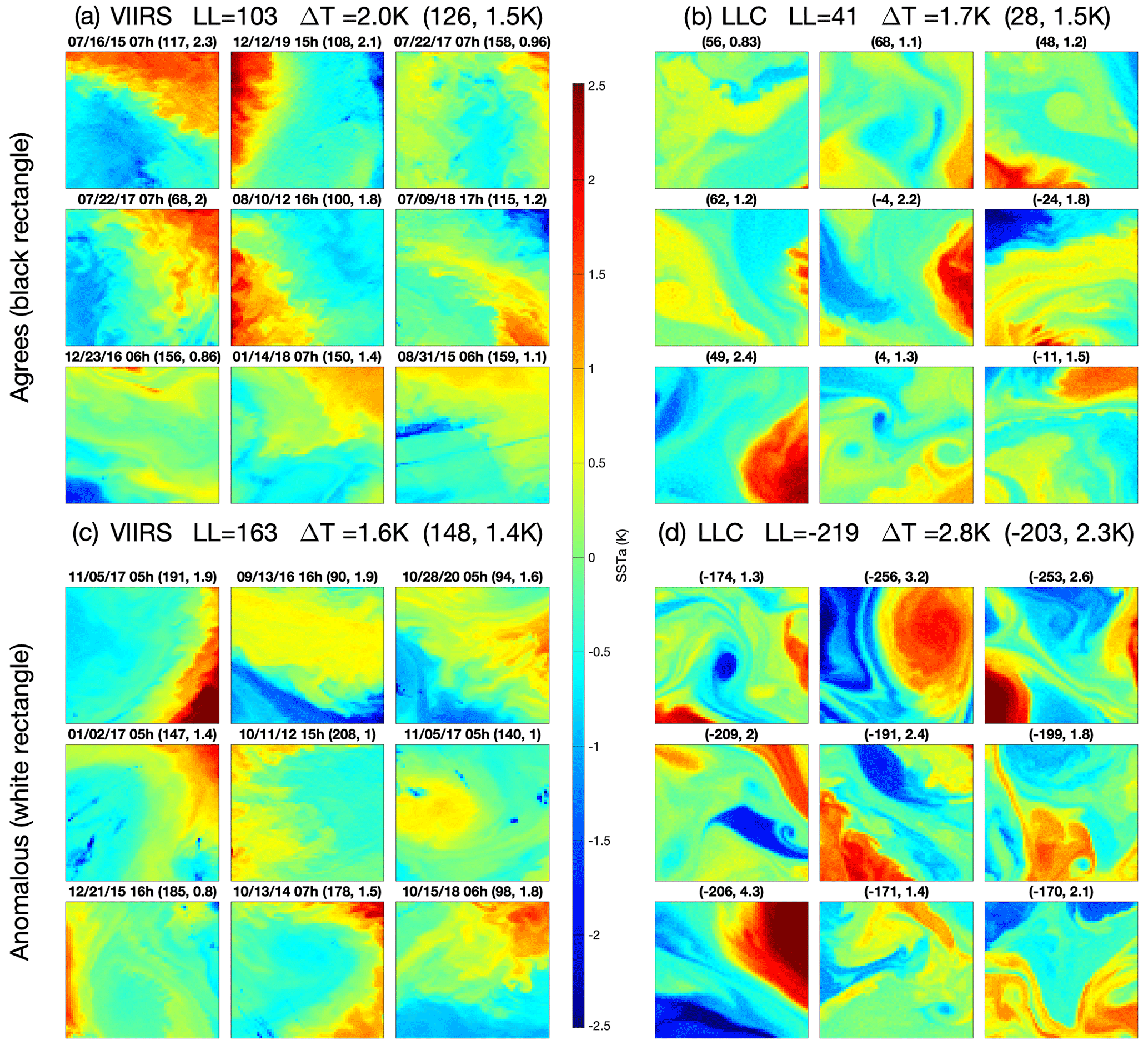
Figure 16(a) Gallery of nine randomly selected VIIRS cutouts within the black rectangle of Fig. 15, the region of “agreement”. (b) Similarly for LLC4320 cutouts in the same region of agreement. (c) VIIRS cutouts in the anomalous region of the white rectangle in Fig. 15. (d) Same as (c) but for LLC4320 cutouts. Dates (month/day/year), times, LL, and ΔT as in Fig. 14.
Gulf Stream
The conclusions for the four possibilities of high values in the Gulf Stream are similar to those for the Southern Ocean.
-
The year simulated, 2012, is atypical, differing from the 2012–2020 mean. This is very unlikely given, as will be shown below, that the modeled Gulf Stream is south of the most extreme southern positions of paths of the Gulf Stream from a number of observational sources.
-
Unresolved clouds exist in the VIIRS fields. This is very unlikely because clouds in the VIIRS fields would tend to increase the structure, i.e., decrease . Hence cloud-free fields would tend to increase , rendering it more anomalous.
-
Noise exists in the VIIRS SST fields. This is unlikely because the geophysical variability in SST in these regions overwhelms noise in the VIIRS fields, but, if it were to contribute, it would again increase , rendering it more anomalous.
-
LLC4320 does not reproduce the submesoscale-to-mesoscale structure well in the Gulf Stream region. As will be shown below, this is likely the cause of the differences, but, unlike the differences in the Southern Ocean, we believe that these differences are due to premature separation of the Gulf Stream from the continental margin; i.e., the Gulf Stream is in the wrong place as opposed to it being in the correct location but too energetic as appears to be the case in the ACC south of Australia.
Figure 17a shows in the Gulf Stream region downstream of the point at which it separates from the continental margin. Figure 17b shows the same data but masked, showing only the HEALPix cells with values exceeding the thresholds identified in Appendix A, ±197. Also shown in these plots is the mean path of the Gulf Stream (magenta line) and its northern and southern extent (black lines). These were determined from manual digitizations of the path of the stream – defined as the maximum cross-stream SST gradient in the vicinity of the stream – in warmest-pixel composites of all AVHRR 1 km SST fields in contiguous 2 d intervals (Lee, 1996). The mean path of the stream was determined by averaging, over all 2 d composites between 1982 and 1999, the point at which these paths intersected integral degrees of longitude. The northern and southern extents are the latitudes for which 99 % of the paths lie to the south – the northern extent – and 99 % lie to the north – the southern extent – for 1982–1999. Large positive differences south of the southern extreme suggest that the LLC4320 output contains more structure in its cutouts than VIIRS, whereas VIIRS fields show more structure within the bounds of the northern and southern extremes.
The large patch of positive values west of 60∘ W corresponds to the premature separation of the modeled Gulf Stream from the continental margin reported by Cornillon and Menemenlis (2018) based on the mean path and extreme envelope of paths shown in Fig. 17 and on the Ocean Surface Current Analyses Real-time (OSCAR) surface currents (https://podaac.jpl.nasa.gov/, last access: 1 November 2023, dataset list; search keywords: oceans, ocean circulation; projects: OSCAR) for 2012. Simply put, the modeled Gulf Stream is found some 250 km to the south of the mean observed stream at 70∘ W and approximately 100 km to the south of the southern extreme observed between 1982 and 1986.
The cause of the positive and negative anomalous values of Fig. 17b become more clear from the individual plots of and in Fig. 17c and d, respectively. The most negative values of are seen in the satellite-derived fields along the edge of the continental slope and, in particular, south of Georges Bank, south of the eastern side of the Gulf of Maine, and south and east of the Grand Banks. (Note that the relatively sharp gradient in values follows the 200 m isobath, shown as dotted red lines in Fig. 17.) Values remain low to the southern extreme of the Gulf Stream. Recall that these HEALPix values are medians obtained from all cutouts in the >8-year interval. During this period the Gulf Stream meanders in the envelope with regions of significant structure at some times and regions of less structure at others, resulting in less structure on average than is found near the shelf break in very active regions that are topographically constrained – south of Georges Bank and south and east of the Grand Banks. The LLC4320 output also shows the most negative values south of Georges Bank but less so south of the Grand Banks. This is likely associated with the premature separation of the stream from the continental margin, the negative values of LL between 65 and 75∘ W and south of about N. Two aspects of interest associated with the model field after separating are (1) the relatively smaller width (meridional extent) of the region covered by the Gulf Stream immediately after separation when compared with the broader distribution associated with the VIIRS data and the rapid increase in LL values – decrease in structure – at approximately 62∘ (the stream appears to die at that point) and (2) the positive LL values east of 60∘ W and south of 33∘ N, the cause of the statistically significant negative differences when compared with the VIIRS results. The former may be due to the fact that model simulation is only for 1 year, while the VIIRS data cover >8 years. The reasons for the rapid die-off of the stream and the relative quietness (larger values of LL) east of 62∘ are not obvious.

Figure 17(a) for the Gulf Stream region after separation from the continental margin. (b) Masked for the same area. (c) . (d) . Thick magenta line shows the mean Gulf Stream path digitized from 2 d AVHRR SST composites for 1982–1999. Thick black lines show the envelope containing 98 % of these paths for the same period, with 1 % of the digitized paths at any given longitude falling shoreward of the envelope and 1 % falling seaward of it. Dotted red line is the 200 m isobath. Red and white rectangles show the focus areas from which galleries of cutouts are selected for Fig. 18.
Next, we examine VIIRS and LLC4320 cutouts inside the Gulf Stream envelope (the white rectangles in Figs. 17c and d at [40–42∘ N, 60–50∘ W] and outside the observed Gulf Stream in the region of anomalously low LLC4320 values associated with the premature separation of the Gulf Stream (the red rectangles in Fig. 17c and d at [34–36∘ N, 70–60∘ W]). Galleries of nine cutouts each for both VIIRS and LLC4320 for both regions are shown in Fig. 18. Cutouts for these galleries were randomly selected as described for the generation of galleries for the equatorial region (Fig. 14). The characteristics of the VIIRS cutouts outside of the Gulf Stream (Fig. 18c) differ substantially from those of the other three galleries, as does the mean LL. VIIRS cutouts within the stream (Fig. 18a) are similar to those in the LLC4320 gallery of cutouts south of the Gulf Stream (Fig. 18d), consistent with the suggestion that the modeled stream separates prematurely from the continental margin. The structure of LLC4320 cutouts in the Gulf Stream (Fig. 18b) lies between that of VIIRS cutouts in the stream (Fig. 18a) and LLC4320 cutouts south of the stream (Fig. 18d), as do the LL values. This is consistent with the modeled stream being to the south of the observed stream.
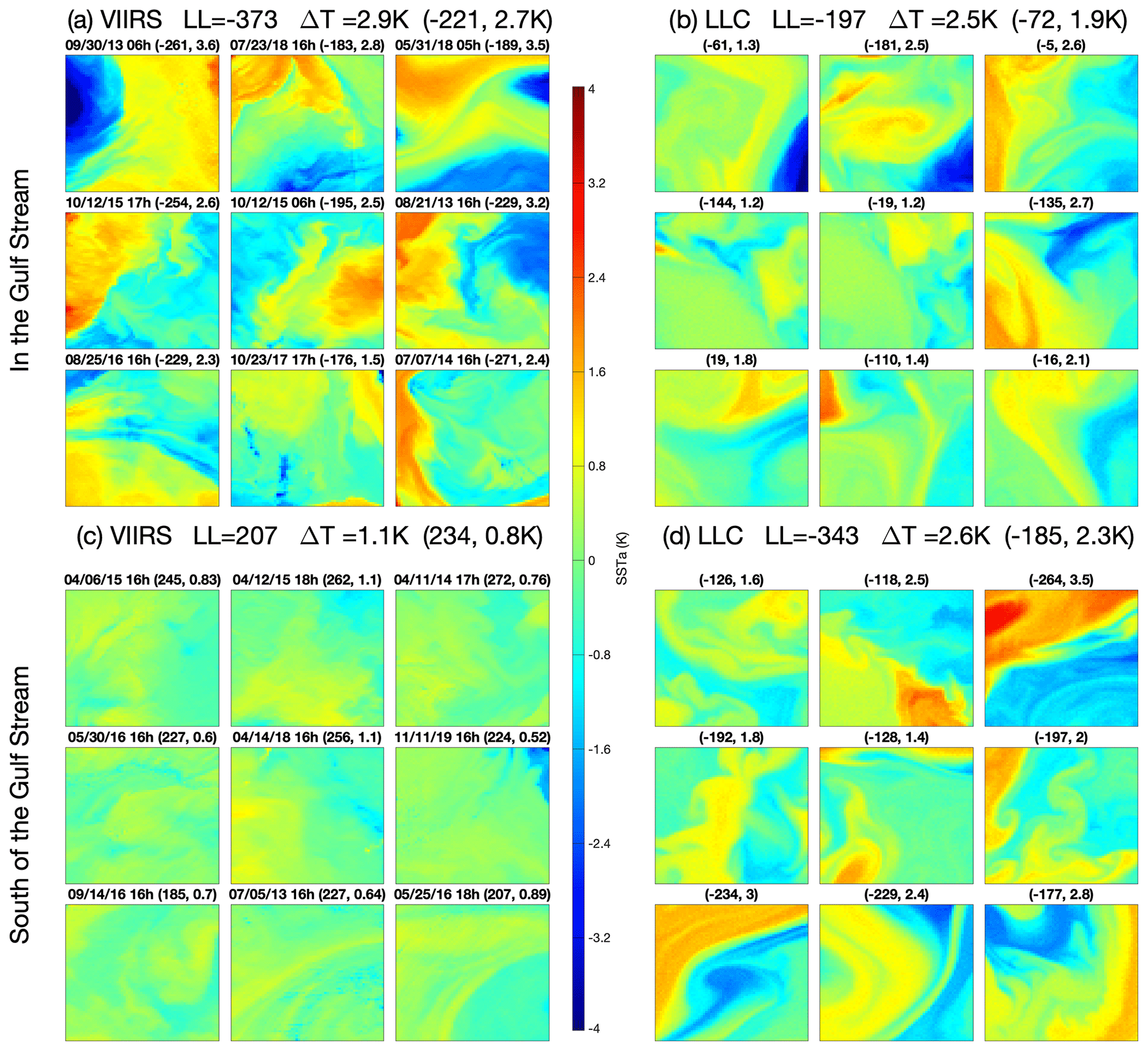
Figure 18(a) Gallery for VIIRS cutouts in the white rectangle of Fig. 17c. (b) Same for LLC4320 cutouts in the white rectangle of Fig. 17d. (c) VIIRS cutouts in the red rectangle of Fig. 17c. (d) LLC4320 cutouts in the red rectangle of Fig. 17d. Dates (month/day/year), times, LL, and ΔT as in Fig. 14.
In this paper we set out to compare outputs from the well-adopted LLC4320 simulation with a large dataset of global observations. Specifically, we have focused on the submesoscale dynamics traced by SST, an observable metric with decades of global coverage provided by a series of sensors on remote sensing satellites. This paper used L2 data from VIIRS, restricted to nearly clear (≥98 % cloud free) cutouts with dimensions of ∼ 150 km × 150 km selected across the ocean.
Our approach for quantitative comparison between data and the model is unconventional. We trained a deep learning probabilistic autoencoder (PAE) on the VIIRS data to learn the distribution of SSTa patterns observed in the ocean and then applied this PAE to geographically and seasonally matched SSTa cutouts from the LLC4320 model. An advantage of this approach is that it is intentionally unsupervised; the network learned from the data the features most characteristic of ocean dynamics traced by SST. On the flip side, the results – especially any differences between data and the model – are more difficult to interpret. The LL metric calculated from the PAE is known to correlate with ΔT and other physical measures of SST yet with significant scatter (Prochaska et al., 2021). And uncertainties are not inherently calculated; instead we have estimated them by applying ULMO to two independent subsets of VIIRS data.
Proceeding in this manner, we found that, in general, the distribution of SSTa patterns present in the VIIRS observations are predicted well by the LLC4320 model (e.g., Fig. 3). Globally, the medians of the LL distributions from VIIRS and LLC4320 agree within 2σ for 65 % of the ocean (Fig. 11). However, there is a modest but significant and latitude-dependent offset between data and the model, with the latter exhibiting less structure in the SSTa cutouts near the Equator and greater structure towards the poles. After correcting for this latitude-dependent offset, we find that the model frequently recovers mesoscale features imprinted in the LL distributions and seen in the field. This includes the reproduction of detailed mesoscale dynamics often forced by deep bathymetric features. We emphasize here that the VIIRS–LLC4320 comparison is being performed on spatial scales of 𝒪(50 km) and less and that it is changes in the structure at these scales that inform the large-scale patterns observed; i.e., the submesoscale structure of cutouts appears to be tied to larger-scale processes. One may conclude that the LLC4320 model has captured salient mesoscale dynamics across the majority of the ocean.
There are, however, a few notable exceptions. One of these is the location of the Gulf Stream, a previously known failure of the LLC4320 simulation (Cornillon and Menemenlis, 2018). Giving confidence to the approach taken in this paper to evaluate the performance of the LLC4320 simulation is the fact that a known region of concern is clearly identified as problematic.
A more subtle difference occurs at the Equator. We have shown from the VIIRS data that the structure in the SSTa cutouts just north of the Equator exceeds that of its southern counterpart (Fig. 14). This difference in SSTa in VIIRS, however, is not reproduced by the LLC4320 simulation, and there is no reason to believe that cross-Equator differences in the VIIRS data are spurious.
Third, we highlighted inconsistencies between the LLC4320 model and VIIRS observations in the ACC, where the former frequently exhibits a higher degree of structure in SST and, presumably, more energetic surface currents. We attribute this increased structure to a misrepresentation of the mixed layer and of subgrid-scale processes that are responsible for energy dissipation and stirring.
We hope that our analysis will inspire similar investigations of both global and regional models. With the construction of large, well-curated datasets, as we have done with VIIRS, one may construct a series of tests. The construction of such a dataset requires intentional decisions on how to extract and preprocess cutouts for direct comparison to model outputs. Furthermore, the data volume of 𝒪(100 TB) is large enough to require best practices with storage, databases, and computing. The authors provide their code (including workflow) with the paper and encourage discussion with parties interested in building their own similar analyses.
We also wish to emphasize several of the weaknesses of our methodology and identify paths for improvement in future work. First, and perhaps foremost, we have not accounted for the mismatch in effective spatial resolution between the model and observations. The pixelization of the L2 VIIRS product is ∼ 750 m at nadir and hence can resolve features in the range of a few kilometers. The LLC4320 simulation, meanwhile, has the finest cell size of ∼ 1 km, but the formulation is not expected to properly resolve features on scales less than 𝒪(10) km (see, e.g., Su et al., 2018). We considered smoothing (i.e., degrading) the VIIRS data to better match the model outputs but were not confident that we could do so with high accuracy. Furthermore, the PAE itself is effectively smoothing the data by passing each cutout through a 512-dimensional bottleneck (e.g., see Fig. 3 of Prochaska et al., 2021).
Related to the above discussion, the initial analysis ignored latitude dependence in the SST structure, despite the predicted and observed dynamical differences driven by geophysical fluid dynamics. Further work might, for example, vary the size of the cutouts proportional to the Rossby radius of deformation. Similarly, if we were to expand the cutout size to larger scales to better assess mesoscale features, it may become necessary to match the orientation of the data (here dictated by the satellite path) with the model (fixed with rows and columns parallel to longitude and latitude).
Another weakness of our implementation is the lack of any error estimation from the PAE outputs (i.e., for individual LL values). This is a general weakness of deep learning algorithms (but see Bayesian neural networks; e.g., Shridhar et al., 2019). Therefore, we approached uncertainty estimation using an empirical estimate generated from subsets of the data (see Appendix A). While effective, it is approximate and relies on the central limit theorem to assume a Gaussian deviate. Relatedly, the LL metric of ULMO has no intrinsically physical, mathematical, or statistical (despite the name) meaning! Future work focused on comparisons of SSTa or other patterns may consider the scattering transform (Mallat, 2012; Cheng and Ménard, 2021), which has a sound mathematical underpinning and may allow for proper statistical tests.
Last, but far from least, are the significant “blemishes” in the data that are absent in the model outputs. Foremost are clouds. The mitigation for clouds adopted here was to (1) limit to cutouts with fewer than 2 % of the pixels masked by the retrieval algorithm (Jonasson et al., 2022) and (2) inpaint these masked pixels. The latter step was required for the PAE and is, in general, required for convolutional neural networks, which expect “complete” fields. In our exploration of the cutouts, however, we identified a high incidence of clouds that were not masked in the VIIRS data. These ranged from minor blemishes in otherwise uniform fields where the clouds generate non-negligible structure (especially evident in Fig. 14a and c) to, in a few cases, corruption of the entire field in the cutout. Another negative consequence, perhaps the most serious, is the terrific reduction in potential data and the resultant geographic biases of the dataset that follow from the 98 % clear criterion (Fig. 1). To the greatest extent possible, future work must continue to identify and mitigate clouds; our own efforts are well underway.
As we conclude, we emphasize that perhaps the greatest value of this paper was the construction and now dissemination of the large dataset of cutouts for comparison with ocean models as well as with other satellite-derived SST datasets. This includes the software to generate and analyze them. All of these products are publicly available as described below.
A question which arises naturally in the context of Fig. 5 is what constitutes a statistically significant difference in between the model output and the VIIRS fields. To address this, the VIIRS dataset is divided into two 4-year segments, 1 February 2012 through 31 January 2016 (referred to as 2012–2015 hereafter) and 1 January 2017 through 31 December 2020 (2017–2020). Subsequently, is calculated for each HEALPix cell for each of the two periods. Figure A1 shows the distribution of cutouts for the first of the two periods. Because the periods for which these data are being calculated are substantially shorter than that of the dataset from which they are drawn (Fig. 1), the number of HEALPix cells with fewer than five cutouts (white in Fig. A1) is substantially larger.
Figure A2 shows a histogram of the differences in the two fields . Also shown in Fig. A2 is the histogram of the differences in the VIIRS and LLC fields, . The two vertical black lines denote ±2σ of the distribution. We use these in the body of the paper to identify significant outliers in the fields. There are three primary contributors to the variance of the distribution. First, there is the uncertainty associated with the assignment of an LL value by the machine learning algorithm to each cutout within the cell; think of this as instrument noise. Second, cutouts in each cell are being sampled from a 3-dimensional space–time region, with the spatial extent defined by the cell boundaries (approximately 100 km on a side) and the temporal extent defined by the 4-year period from which each distribution is drawn; think of this as the uncertainty in estimated values based on the finite sample size. Third is the difference in the value between the period covered by the two datasets, i.e., the true geophysical difference. For , the latter is the difference between 2012–2015 and 2017–2020. For this would be the difference between the simulated period, 2012, and the period from which the VIIRS data are sampled, 2012–2020. This means that the variability in places an upper bound on uncertainty in the LL values, variability which is due to the position within the cell and the period from which cutouts contributing to the cell are drawn. As shown in the next paragraph, we believe that the geophysical contribution of uncertainty to the differences is small; hence the variability in is a good measure of what constitutes a significant deviation between two datasets. In light of this, we will use 2 standard deviations of the distribution to identify regions in which the model output agrees/disagrees with the satellite-derived fields.
Also of importance in understanding the significance of differences between is the degree to which these differences are distributed geographically. Specifically, shifts in major ocean currents as well as changes in forcing from one period to another could result in different structures in the submesoscale-to-mesoscale range, which would display as geographic regions of positive or negative differences between two periods. Figure A3 suggests that, with a few exceptions, the distribution of is, in fact, quite random; i.e., at least for this pair of 4-year periods, the differences in submesoscale-to-mesoscale structure is relatively random. There are, however, some regions of more than a few HEALPix cells which stand out as significantly different between the two periods in either the positive or negative sense. A narrow negative band is evident along the northern edge of the ACC south of the Indian Ocean, suggesting that the ACC may have shifted south between 2012–2015 and 2017–2020 – more negative values of the difference correspond to less structure in the second period.
Significant differences are also evident in the vicinity of the Gulf Stream and Kuroshio (Fig. A4b masked to show only HEALPix cells with values more than 2 standard deviations from the mean, i.e., significant outliers). Figure A4a shows the distribution for 2012–2015 (the geographic distribution of for 2017–2020 is virtually indistinguishable from that shown for 2012–2015 in this plot). The dark-blue areas on the western side of the North Atlantic and North Pacific north of approximately 35∘ N correspond to a significant structure in the SST fields in and north of the associated western boundary currents – the Gulf Stream and Kuroshio – an observation documented in Prochaska et al. (2021). The region of enhanced differences between the two periods appears to be on the northern edge and to the north of these currents. Figure A5 is a blown-up image of the region in the vicinity of the Gulf Stream: Fig. A5a shows the unmasked values, and Fig. A5b shows the masked values. The more positive differences north of the Gulf Stream mean path (magenta line in the figure) suggest an increase in structure in 2017–2020 compared with that in 2012–2015. That much of the differences are north of the northernmost extent of the Gulf Stream (upper black line) argues not only that has the mean path of the stream likely moved to the north in this period but also that this displacement resulted in more submesoscale-to-mesoscale turbulence in the region north of the stream. Of particular interest, although not the focus of this paper, is the similarity in the patterns in the vicinity of the Kuroshio, suggesting that the phenomena is hemispheric as opposed to confined to one ocean basin. The point here is that, although there are some regions of significant differences, these tend to be relatively small and are, in general, associated with strong currents – the Gulf Stream, the Kuroshio, and the ACC.
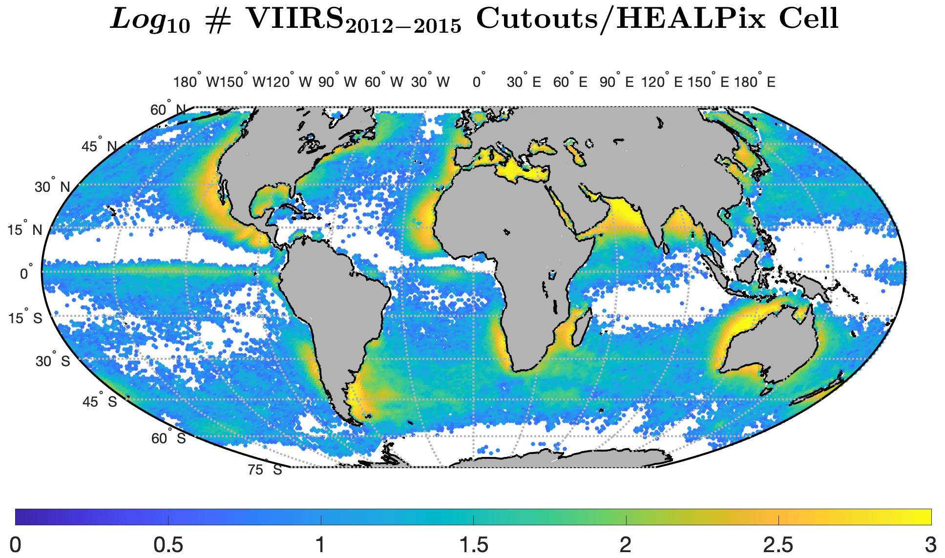
Figure A1Number of VIIRS cutouts per HEALPix cell for the period 2012–2015. HEALPix cells with fewer than five cutouts for 2012–2015 or fewer than five cutouts for 2017–2020 are shown in white.
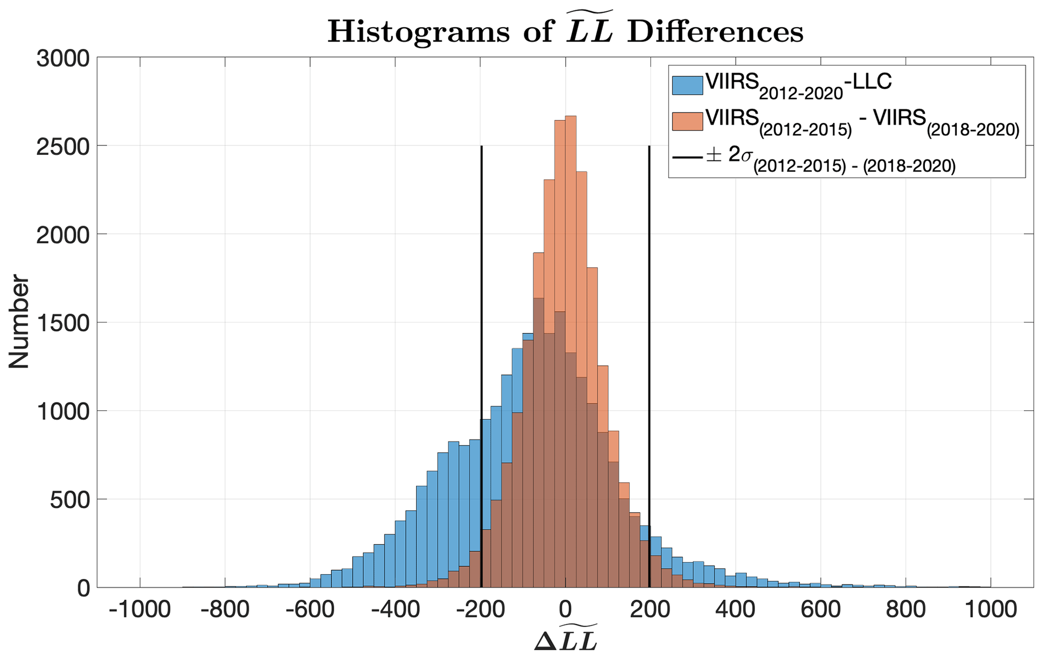
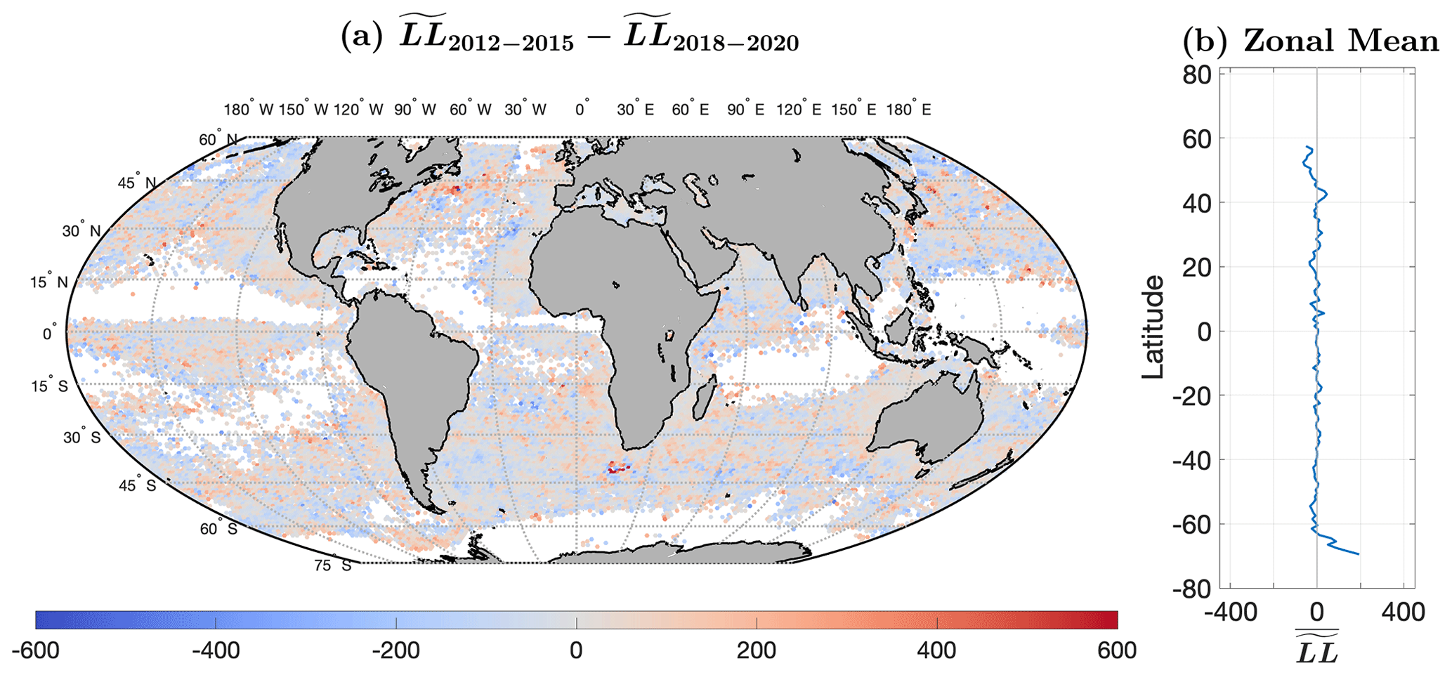
Figure A3(a) . White areas show fewer than five cutouts in the corresponding HEALPix cell in 2012–2015 and/or 2017–2020. The same color palette is used in this figure as in Fig. 5 to facilitate comparison as well as to emphasize the significant differences in . (b) Zonal mean of (a).
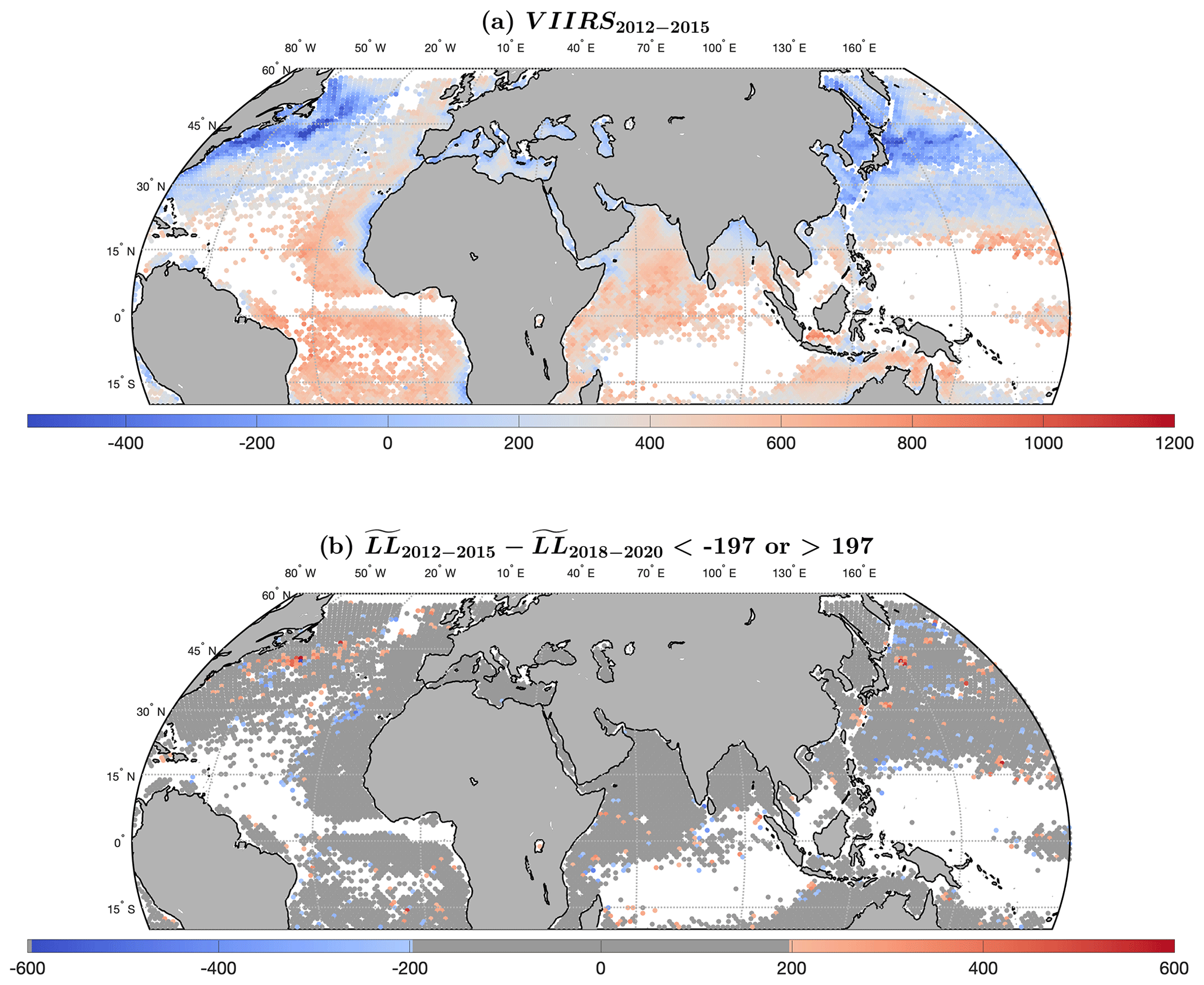
Figure A4(a) for the Northern Hemisphere. (b) Masked . Dark gray: |. Light gray: land. White: fewer than five cutouts per HEALPix cell for both 2012–2015 and 2017–2020.
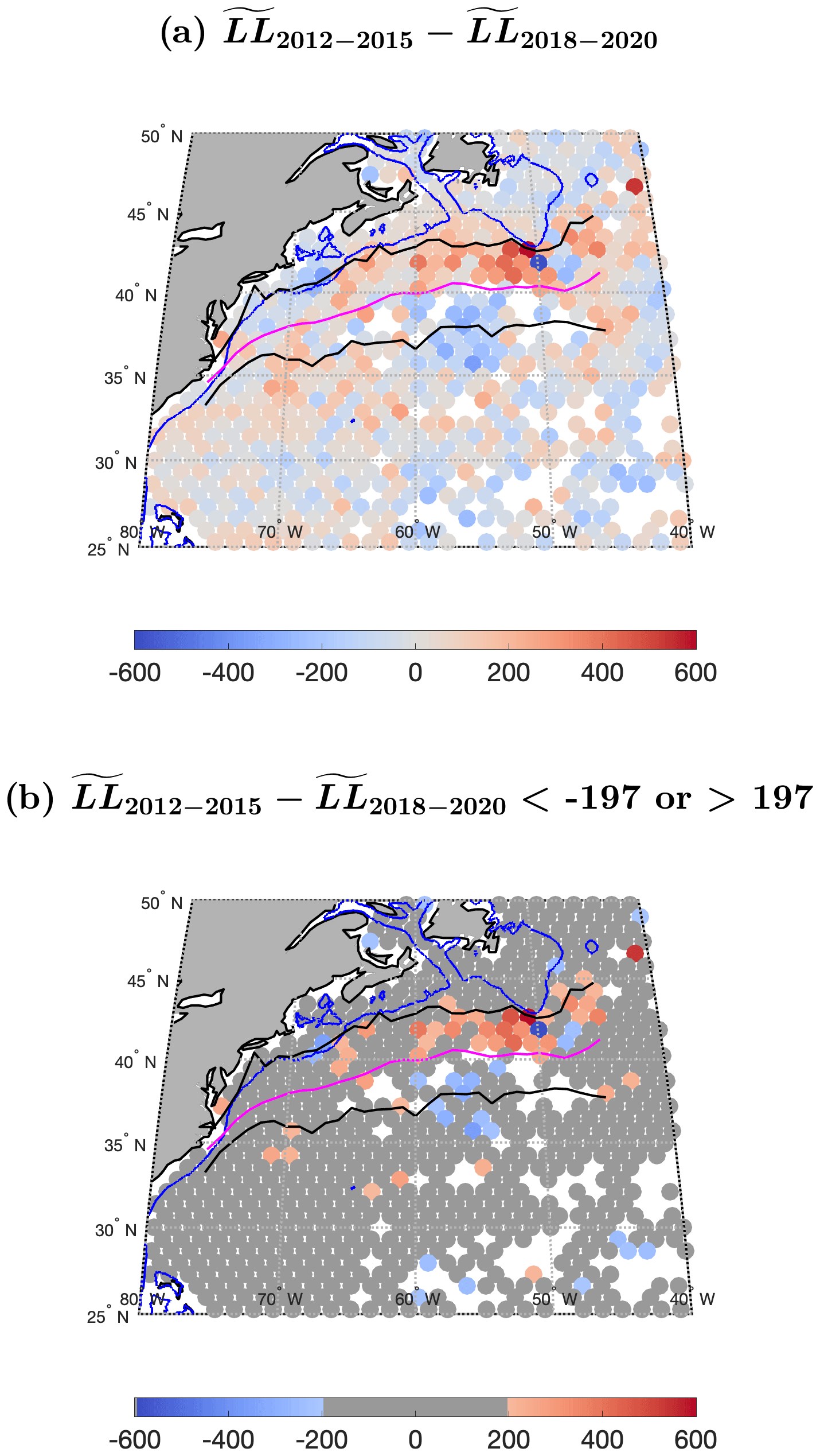
Figure A5(a) As in Figs. A3 and A4 but focused on the Gulf Stream region. (b) Masked version of (a). Magenta line between approximately 75 and 45∘ W is the mean path of the Gulf Stream digitized from 2 d composites of 1 km AVHRR SST fields for 1982–1999. Black lines are for the northernmost and southernmost extents of Gulf Stream paths digitized from the same dataset as (a) but for 1982–1986.
| ACC | Antarctic Circumpolar Current |
| AVHRR | Advanced Very High Resolution Radiometer |
| ECCO | Estimating the Circulation and Climate of the Ocean |
| ECMWF | European Centre for Medium-Range Weather Forecasts |
| GHRSST | Group for High Resolution Sea Surface Temperature |
| HEALPix | Hierarchical Equal Area isoLatitude Pixelation |
| JPL | Jet Propulsion Laboratory |
| L2 | Level-2 |
| L2P | Level-2P |
| LL | Log likelihood |
| LLC | Latitude–longitude–polar cap |
| LLC4320 | Latitude–longitude–polar cap 4320 |
| LLC2160 | Latitude–longitude–polar cap 2160 |
| LLC1080 | Latitude–longitude–polar cap 1080 |
| MITgcm | MIT General Circulation Model |
| MIT | Massachusetts Institute of Technology |
| MODIS | Moderate Resolution Imaging Spectroradiometer |
| NASA | National Aeronautics and Space Administration |
| NOAA | National Oceanic and Atmospheric Administration |
| NPP | National Polar-orbiting Partnership |
| NSF | National Science Foundation |
| OGCM | Ocean general circulation model |
| OSCAR | Ocean Surface Current Analyses Real-time |
| PAE | Probabilistic autoencoder |
| PO.DAAC | Physical Oceanography Distributed Active Archive Center |
| RAN2 | Second full-mission reanalysis |
| SLSTR | Sea and Land Surface Temperature Radiometer |
| SST | Sea surface temperature |
| SSTa | Sea surface temperature anomaly |
| SURFO | Summer Undergraduate Research Fellowships in Oceanography |
| URI | University of Rhode Island |
| VIIRS | Visible Infrared Imaging Radiometer Suite |
All of the data generated and analyzed in this paper are publicly available as Parquet tables and HDF5 files at Dryad (https://doi.org/10.7291/D1DM5F, Prochaska et al., 2023a). The code developed throughout the project is provided at https://doi.org/10.5281/zenodo.8325304 (Prochaska et al., 2023b) or at https://github.com/AI-for-Ocean-Science/ulmo (last access: 1 November 2023).
KG performed the initial studies on which this paper is based. KG, JXP, and PC contributed to the subsequent analyses of the data. All contributed to the writing of the paper, which was led by KG. Figures were generated by KG and PC. JXP provided input on the machine learning portion of the project. PC and DM provided input related to physical oceanography. PC provided the satellite data expertise. DM provided the modeling expertise. MK and JXP processed the satellite data.
The contact author has declared that none of the authors has any competing interests.
Publisher's note: Copernicus Publications remains neutral with regard to jurisdictional claims made in the text, published maps, institutional affiliations, or any other geographical representation in this paper. While Copernicus Publications makes every effort to include appropriate place names, the final responsibility lies with the authors.
J. Xavier Prochaska acknowledges future support from the Simons Foundation and the University of California, Santa Cruz. DM carried out research at the Jet Propulsion Laboratory, California Institute of Technology, under a contract with NASA, with support from the Physical Oceanography (PO) and Modeling, Analysis, and Prediction (MAP) programs. Katharina Gallmeier was supported during the summer of 2021 through the Summer Undergraduate Research Fellowships in Oceanography program of the University of Rhode Island (funded by the NSF). Support for Peter Cornillon was provided by the Office of Naval Research (ONR), NASA, and the state of Rhode Island.
The VIIRS L2 SST data were provided by the Group for High Resolution Sea Surface Temperature and the National Oceanic and Atmospheric Administration and obtained from the National Aeronautics and Space Administration Physical Oceanography Distributed Active Archive Center. The LLC4320 SST fields were obtained via the xmitgcm package obtained at https://xmitgcm.readthedocs.io/en/latest/ (last access: 1 November 2023).
Some of the results in this paper have been derived using HEALPix (Górski et al., 2005). The authors acknowledge use of the Nautilus cloud computing system, which is supported by the US National Science Foundation (NSF). High-end computing for the LLC4320 simulation was provided by the NASA Advanced Supercomputing (NAS) Division at the Ames Research Center.
This research has been supported by the Office of Naval Research (grant no. N00014-17-1-2963), the National Aeronautics and Space Administration (grant nos. 80NSSC18K0837 and 80NSSC20K1728), and the National Science Foundation (grant nos. OCE-1950586, CNS-1456638, CNS-1730158, CNS-2100237, CNS-2120019, ACI-1540112, ACI-1541349, OAC-1826967, and OAC-2112167).
This paper was edited by Riccardo Farneti and reviewed by Takaya Uchida and one anonymous referee.
Arbic, B. K., Alford, M. H., Ansong, J. K., Buijsman, M. C., Ciotti, R. B., Farrar, J. T., Hallberg, R. W., Henze, C. E., Hill, C. N., Luecke, C. A., Menemenlis, D., Metzger, E. J., Müeller, M., Nelson, A. D., Nelson, B. C., Ngodock, H. E., Ponte, R. M., Richman, J. G., Savage, A. C., Scott, R. B., Shriver, J. F., Simmons, H. L., Souopgui, I., Timko, P. G., Wallcraft, A. J., Zamudio, L., and Zhao, Z.: A Primer on Global Internal Tide and Internal Gravity Wave Continuum Modeling in HYCOM and MITgcm, in: New Frontiers in Operational Oceanography, edited by: Chassignet, E. P., Pascual, A., Tintoré, J., and Verron, J., Chap. 13, GODAE OceanView, 307–392, https://doi.org/10.17125/gov2018.ch13, 2018. a, b
Arbic, B. K., Elipot, S., Brasch, J. M., Menemenlis, D., Ponte, A. L., Shriver, J. F., Yu, X., Zaron, E. D., Alford, M. H., Buijsman, M. C., Abernathey, R., Garcia, D., Guan, L., Martin, P. E., and Nelson, A. D.: Near‐Surface Oceanic Kinetic Energy Distributions From Drifter Observations and Numerical Models, J. Geophys. Res.-Oceans, 127, 1–30, https://doi.org/10.1029/2022JC018551, 2022. a
Bryan, K.: Michael Cox (1941–1989): His Pioneering Contributions to Ocean Circulation, J. Phys. Oceanogr., 21, 1259–1270, 1991. a
Böhm, V. and Seljak, U.: Probabilistic Auto-Encoder, ArXiv [preprint], https://doi.org/10.48550/arXiv.2006.05479, 2020. a
Cheng, S. and Ménard, B.: How to quantify fields or textures? A guide to the scattering transform, arXiv [preprint], https://doi.org/10.48550/arXiv.2112.01288, 2021. a
Cornillon, P. and Menemenlis, D.: The Gulf Stream: Yikes, What's It Doing Down There?, in: ECCO Project Meeting 2018, Austin, Texas, USA, https://www.ecco-group.org/meetings-documents.htm?id=ecco2018 (last access: 1 November 2023), 2018. a, b
Cox, M. D.: A Baroclinic Model of the World Ocean: Preliminary Results, in: Numerical Models of the Ocean Circulation, National Academy of Sciences, Washington, D.C., 107–118, ISBN 10 0309022258, SBN 13 9780309022255, 1975. a
Dushaw, B. D. and Menemenlis, D.: Resonant Diurnal Internal Tides in the North Atlantic: 2. Modeling, Geophys. Res. Lett., 50, 2189–2192, https://doi.org/10.1029/2022GL101193, 2023. a
Flexas, M. M., Schodlok, M. P., Padman, L., Menemenlis, D., and Orsi, A. H.: Role of tides on the formation of the Antarctic Slope Front at the Weddell-Scotia Confluence J. Geophys. Res.-Oceans, 120, 3658–3680, 2015. a
Forget, G., Campin, J.-M., Heimbach, P., Hill, C. N., Ponte, R. M., and Wunsch, C.: ECCO version 4: an integrated framework for non-linear inverse modeling and global ocean state estimation, Geosci. Model Dev., 8, 3071–3104, https://doi.org/10.5194/gmd-8-3071-2015, 2015. a
Fox-Kemper, B., Adcroft, A., Böning, C. W., Chassignet, E. P., Curchitser, E., Danabasoglu, G., Eden, C., England, M. H., Gerdes, R., Greatbatch, R. J., Griffies, S. M., Hallberg, R. W., Hanert, E., Heimbach, P., Hewitt, H. T., Hill, C. N., Komuro, Y., Legg, S., Le Sommer, J., Masina, S., Marsland, S. J., Penny, S. G., Qiao, F., Ringler, T. D., Treguier, A. M., Tsujino, H., Uotila, P., and Yeager, S. G.: Challenges and Prospects in Ocean Circulation Models, Front. Mar. Sci., 6, 65, https://doi.org/10.3389/fmars.2019.00065, 2019. a
Górski, K. M., Hivon, E., Banday, A. J., Wandelt, B. D., Hansen, F. K., Reinecke, M., and Bartelmann, M.: HEALPix: A Framework for High-Resolution Discretization and Fast Analysis of Data Distributed on the Sphere, Astrophys. J., 622, 759–771, https://doi.org/10.1086/427976, 2005. a, b
Hill, C., Menemenlis, D., Ciotti, B., and Henze, C.: Investigating solution convergence in a global ocean model using a 2048-processor cluster of distributed shared memory machines, Sci. Programm., 15, 107–115, 2007. a
Jonasson, O. and Ignatov, A.: Status of second VIIRS reanalysis (RAN2), in: Ocean Sensing and Monitoring XI, edited by: Hou, W. W. and Arnone, R. A., International Society for Optics and Photonics, SPIE, Vol. 11014, p. 110140O, https://doi.org/10.1117/12.2518908, 2019. a
Jonasson, O., Ignatov, A., Pryamitsyn, V., Petrenko, B., and Kihai, Y.: JPSS VIIRS SST Reanalysis Version 3, Remote Sens., 14, 3476, https://doi.org/10.3390/rs14143476, 2022. a, b
Lee, T.: Propagation of Gulf Stream Meanders between 74 and 70 W, J. Phys. Oceanogr., 26, 205–224, 1996. a
Leroux, S., Brankart, J.-M., Albert, A., Brodeau, L., Molines, J.-M., Jamet, Q., Le Sommer, J., Penduff, T., and Brasseur, P.: Ensemble quantification of short-term predictability of the ocean dynamics at a kilometric-scale resolution: a Western Mediterranean test case, Ocean Sci., 18, 1619–1644, https://doi.org/10.5194/os-18-1619-2022, 2022. a
Light, C. X., Arbic, B. K., Martin, P. E., Brodeau, L., Farrar, J. T., Griffies, S. M., Kirtman, B. P., Laurindo, L. C., Menemenlis, D., Molod, A., Nelson, A. D., Nyadjro, E., O'Rourke, A. K., Shriver, J. F., Siqueira, L., Small, R. J., and Strobach, E.: Effects of grid spacing on high-frequency precipitation variance in coupled high-resolution global ocean–atmosphere models, Clim. Dynam., 59, 2887–2913, https://doi.org/10.1007/s00382-022-06257-6, 2022. a
Mallat, S.: Group Invariant Scattering, Commun. Pure Appl. Math., 65, 1331–1398, https://doi.org/10.1002/cpa.21413, 2012. a
Marshall, J., Adcroft, A., Hill, C., Perelman, L., and Heisey, C.: A finite-volume, incompressible Navier Stokes model for studies of the ocean on parallel computers, J. Geophys. Res.-Oceans, 102, 5753–5766, https://doi.org/10.1029/96JC02775, 1997. a
Menemenlis, D., Campin, J.-M., Heimbach, P., Hill, C. N., Lee, T., Nguyen, A. T., Schodlok, M. P., and Zhang, H.: ECCO2: High resolution global ocean and sea ice data synthesis, Mercator Ocean Quarterly Newsletter, 31, 13–21, 2008. a
NOAA Satellite Applications and Research (STAR), GHRSST Level 2P NOAA STAR SST v2.80 from VIIRS on S-NPP Satellite, PO.DAAC [data set], https://doi.org/10.5067/GHVRS-2PO28, 2021. a
Papamakarios, G., Nalisnick, E., Rezende, D. J., Mohamed, S., and Lakshminarayanan, B.: Normalizing Flows for Probabilistic Modeling and Inference, ArXiv [preprint], https://doi.org/10.48550/ARXIV.1912.02762, 2019. a
Prochaska, J. X., Cornillon, P. C., and Reiman, D. M.: Deep Learning of Sea Surface Temperature Patterns to Identify Ocean Extremes, Remote Sens., 13, 744, https://doi.org/10.3390/rs13040744, 2021. a, b, c, d, e, f, g, h, i, j
Prochaska, J. X., Gallmeier, K., Cornillon, P., Menemenlis, D., and Kelm, M.: VIIRS data and Ulmo model for comparison to the LLC4320 ECCO ocean general circulation model, Dryad [data set], https://doi.org/10.7291/D1DM5F, 2023a. a
Prochaska, J. X., Guo, E., aagabin, BenPritikin, mskelm, Cornillon, P., Reiman, D., and vgotov2: AI-for-Ocean-Science/ulmo: Updates for Gallmeier in press, Zenodo [code], https://doi.org/10.5281/zenodo.8325304, 2023b. a
Rocha, C. B., Chereskin, T. K., Gille, S. T., and Menemenlis, D.: Mesoscale to Submesoscale Wavenumber Spectra in Drake Passage, J. Phys. Oceanogr., 46, 601–620, https://doi.org/10.1175/JPO-D-15-0087.1, 2016a. a
Rocha, C. B., Gille, S. T., Chereskin, T. K., and Menemenlis, D.: Seasonality of submesoscale dynamics in the Kuroshio Extension, Geophys. Res. Lett., 43, 11304–11311, https://doi.org/10.1002/2016GL071349, 2016b. a
Shridhar, K., Laumann, F., and Liwicki, M.: A Comprehensive guide to Bayesian Convolutional Neural Network with Variational Inference, ArXiv [preprint], https://doi.org/10.48550/ARXIV.1901.02731, 2019. a
Su, Z., Wang, J., Klein, P., Thompson, A. F., and Menemenlis, D.: Ocean submesoscales as a key component of the global heat budget, Nat. Commun., 9, 1–8, https://doi.org/10.1038/s41467-018-02983-w, 2018. a
Torres, H. S., Klein, P., Wang, J., Wineteer, A., Qiu, B., Thompson, A. F., Renault, L., Rodriguez, E., Menemenlis, D., Molod, A., Hill, C. N., Strobach, E., Zhang, H., Flexas, M., and Perkovic-Martin, D.: Wind work at the air-sea interface: a modeling study in anticipation of future space missions, Geosci. Model Dev., 15, 8041–8058, https://doi.org/10.5194/gmd-15-8041-2022, 2022. a
Uchida, T., Le Sommer, J., Stern, C., Abernathey, R. P., Holdgraf, C., Albert, A., Brodeau, L., Chassignet, E. P., Xu, X., Gula, J., Roullet, G., Koldunov, N., Danilov, S., Wang, Q., Menemenlis, D., Bricaud, C., Arbic, B. K., Shriver, J. F., Qiao, F., Xiao, B., Biastoch, A., Schubert, R., Fox-Kemper, B., Dewar, W. K., and Wallcraft, A.: Cloud-based framework for inter-comparing submesoscale-permitting realistic ocean models, Geosci. Model Dev., 15, 5829–5856, https://doi.org/10.5194/gmd-15-5829-2022, 2022. a
van der Walt, S., Schönberger, J. L., Nunez-Iglesias, J., Boulogne, F., Warner, J. D., Yager, N., Gouillart, E., Yu, T., and the scikit-image contributors: scikit-image: image processing in Python, PeerJ, 2, e453, https://doi.org/10.7717/peerj.453, 2014. a
Wu, F., Cornillon, P., Boussidi, B., and Guan, L.: Determining the Pixel-to-Pixel Uncertainty in Satellite-Derived SST Fields, Remote Sens., 9, 877, https://doi.org/10.3390/rs9090877, 2017. a, b
Xu, Y., Rignot, E., Fenty, I., Menemenlis, D., and Flexas, M. M.: Subaqueous melting of Store Glacier, west Greenland from three-dimensional, high-resolution numerical modeling and ocean observations, Geophys. Res. Lett., 40, 4648–4653, https://doi.org/10.1002/grl.50825, 2013.
Yu, X., Ponte, A. L., Elipot, S., Menemenlis, D., Zaron, E. D., and Abernathey, R.: Surface Kinetic Energy Distributions in the Global Oceans From a High‐Resolution Numerical Model and Surface Drifter Observations, Geophys. Res. Lett., 46, 9757–9766, https://doi.org/10.1029/2019GL083074, 2019. a
The Advanced Very High Resolution Radiometer (AVHRR) is not a multi-detector instrument, so it does not suffer from the striping and geometric distortion issues associated with data from VIIRS, but the coarser spatial resolution, 1.1 km at nadir, introduces greater degradation in resolution with distance from nadir and the noisier instrument results in a product with at least twice the noise of VIIRS (Wu et al., 2017). The Sea and Land Surface Temperature Radiometer (SLSTR) instrument carried on the European Sentinel satellites provides an interesting alternative dataset, but, given our lack of detailed familiarity with these data, we elected to continue using VIIRS.