An emulation-based approach for interrogating reactive transport models

We present an emulation-based approach to understand the interactions among different chemical and biological processes modelled in environmental reactive transport models (RTMs) and explore how the parameterisation of these processes influences the results of multi-component RTMs. We utilise a previously published RTM consisting of 20 primary species, 20 secondary complexes, 17 mineral reactions, and 2 biologically mediated reactions; this RTM describes bio-stimulation using sediment from a contaminated aquifer. We choose a subset of the input parameters to vary over a range of values. The result is the construction of a new dataset that describes the model behaviour over a range of environmental conditions. Using this dataset to train a statistical model creates an emulator of the underlying RTM. This is a condensed representation of the original RTM that facilitates rapid exploration of a broad range of environmental conditions and sensitivities. As an illustration of this approach, we use the emulator to explore how varying the boundary conditions in the RTM describing the aquifer impacts the rates and volumes of mineral precipitation. A key result of this work is the recognition of an unanticipated dependency of pyrite precipitation on pCO₂ in the injection fluid due to the stoichiometry of the microbially mediated sulfate reduction reaction. This complex relationship was made apparent by the emulator, while the underlying RTM was not specifically constructed to create such a feedback. We argue that this emulation approach to sensitivity analysis for RTMs may be useful in discovering such new coupled sensitives in geochemical systems and for designing experiments to optimise environmental remediation. Finally, we demonstrate that this approach can maximise specific mineral precipitation or dissolution reactions by using the emulator to find local maxima, which can be widely applied in environmental systems.

1 Introduction

Reactive transport modelling has been extensively applied across a wide variety of environmental systems, providing a powerful means of quantifying and even predicting processes across Earth's (near-) surface environments (Richter and DePaolo, 1987; Bain et al., 2000; Johnson et al., 2004; van Breukelen et al., 2004; Gaus et al., 2005; Torres et al., 2015; Li et al., 2017; Arora et al., 2020; Molins and Knabner, 2020; Rolle and Borgne, 2020; Druhan et al., 2020; Cama et al., 2020). Reactive transport models (RTMs) are constructed by combining multiple physical, chemical, and biological processes to simulate the behaviour of environmental systems. As applications and software have concurrently expanded (Steefel et al., 2015; Li et al., 2017; Maher and Mayer, 2019; Druhan and Tournassatt, 2019), it is becoming increasingly common to explicitly calculate the rates of production and consumption for a variety of coexisting chemical species, as well as their equilibria with mineral phases and their transport as they evolve in time and space. This type of multi-phase, multi-component RTM is a type of forward modelling where the results of the simulation emerge from a complex suite of interacting pathways; hence, the causes of observed behaviour are not always obvious.

RTMs are often designed to describe the behaviour of specific field sites and systems. Due to their process-based nature, designing RTMs requires selection of a suite of chemical reactions and transport mechanisms which are thought to dominate the geochemistry of the system over the scales of interest. However, the parameterisation of various selected processes is often not unique and can impact system behaviour (Williams et al., 2011; Martinez et al., 2014; Seigneur et al., 2021; Steefel et al., 2005a). To assess the impact of the choice of parameterisation and the values chosen for different parameters on model predictions, sensitivity analyses are generally performed (Malaguerra et al., 2013; Gatel et al., 2019). However, as RTMs become increasingly sophisticated, they incorporate disparate processes that can interact with each other in complex ways (Dwivedi et al., 2018; Hubbard et al., 2018, 2019; Maavara et al., 2021a, b; Dwivedi et al., 2017).

The sensitivity analysis of an RTM in an application to a specific environmental system can elucidate the relative importance of specific interactions – for example, testing the solubility of mineral phases relative to changes in the solution chemistry. However, results might emerge that were not anticipated. These results might represent real but unexpected interactions, in which case the sensitivity analysis has yielded new insights into the system being modelled. Equally, the result might represent an incorrect interaction between two different processes that are known to act independently of each other, in which case the RTM can be improved. Unfortunately, due to the computational expense of many modern multi-component RTMs (e.g. Abd and Abushaikha, 2021; Seigneur et al., 2021; Gharasoo et al., 2022), it is normally impractical to perform sensitivity analyses in more than a few dimensions, and it is up to the investigator to use their knowledge of the system to choose which sensitivity analyses are necessary to explore (Steefel et al., 2005b). Ideally, we would be able to systematically perform sensitivity analyses over many model parameters considering how model outputs vary as a function of multiple input parameters simultaneously (i.e. in a multivariate way) while also lightening the computational burden that commonly occurs when using inverse modelling approaches implemented by codes like PEST and iTOUGH2 (Doherty, 2004; Finsterle et al., 2017). Such a capacity could direct future laboratory-based investigations to test whether these model results are real-world phenomena, ultimately offering improved parameterisation of critical components within the reaction network.

Here, we demonstrate a method for exploring a wide variety of potential model parameters by adopting an emulator-based approach. Ours is not the first work to apply emulators to RTM simulations. Notably, a rich vein of research based around replacing the geochemical solver in RTMs with an emulator has emerged over the past few years (see Laloy and Jacques (2021) and Kyas et al. (2022), among others). However, the work presented here is less concerned with speeding up individual RTM simulations as it is with developing new methods to explore geochemical parameter spaces. We also investigate the effect of changing geochemical parameters on the overall outcome of RTM simulations, with an eye towards predicting system outcomes in real-world scenarios. This is similar in nature to recent work conducted by Ahmmed et al. (2021), which explores the ability of different machine learning methods to predict the degree of mixing and the progression of a simplified, generic reaction (A + B → C) in a finite-element simulation, and we extend the idea of predicting the final state of a simulation to published RTMs describing real-world systems.

Such emulation approaches in predicting the outcomes of physical systems have a long history, including applications in physics-based animation (Grzeszczuk et al., 1998), complex multi-physics simulators (Lu et al., 2021; Bianchi et al., 2016), climate models (Beucler et al., 2019; Krasnopolsky et al., 2005; Castruccio et al., 2014; Kashinath et al., 2021), and emulating fluid flow through dolomite using a neural network (Li et al., 2022). In an emulator approach, the underlying physical system is approximated by a statistical model (the emulator) which can be evaluated more quickly than a conventional forward model. How this emulator is constructed varies by implementation and may encode assumptions about the underlying system to be modelled (e.g. conservation of energy; Beucler et al., 2019). In this study, we are primarily interested in exploring and emulating the geochemical behaviour of RTMs; therefore, we focus less on transport effects and restrict ourselves to emulating one-dimensional RTMs.

In our implementation, the emulator is built by training a gradient-boosted trees (GBT) regressor (Chen et al., 2016) on a synthetic dataset generated from the original RTM. By training such a GBT model on the synthetic dataset generated by the original RTM, we create an emulator of the original system. This emulation approach is general and can be applied to a wide range of RTMs using off-the-shelf statistical libraries and requiring no special construction of the statistical model beyond the choice of some training parameters. This approach can identify the critical processes and parameters within RTMs and address the requirement for comprehensive, multivariate sensitivity analyses.

We first present a tool that automates the creation of synthetic datasets: a Python wrapper for the RTM software CrunchTope (Druhan et al., 2013; Steefel et al., 2015), which we have named Omphalos. Omphalos edits and runs CrunchTope input files in an automated fashion, systematically changing model parameters according to user specification. It then records the output data, along with the corresponding model input parameters, for later analysis. We then apply a machine learning method (gradient-boosted trees) to these recorded inputs and outputs to create a predicative model that can reproduce RTM outputs based on the input variables, which we term a reactivate transport emulator (RTE).

We suggest that our contribution to the development of reactive transport emulators could be used to direct new experimental investigation to identify and corroborate predicted dependencies, providing multivariate analysis of RTMs and helping to identify effects that can, in the future, be considered explicitly when developing new RTMs. In pursuit of this goal, we demonstrate our emulator approach in an application to an RTM built for biostimulation of a contaminated aquifer. We also show an additional application of this approach to efficiently predict the condition which maximises an RTM-predicted time-integrated rate over the set of chosen parameters. We also present, in the Supplement, another example in an application to a deep-sea sediment column.

2 Description of the case study

Old Rifle site, Colorado

The Old Rifle site is located near Rifle, Colorado, USA. The location historically hosted a vanadium- and uranium-ore-processing facility, and the groundwater at the site remains high in aqueous uranium. Oxidised uranium (U(VI)) is fluid mobile and highly toxic, while reduced uranium (U(IV)) is much less soluble and forms stable precipitates such as uraninite (UO₂) (Anderson et al., 2003; Wu et al., 2006; Dullies et al., 2010; Williams et al., 2011; Long et al., 2015). Thus, uranium reduction has been suggested as a means for remediating uranium contamination in groundwater. It has been shown that iron sulfide minerals (FeS_2(s)) aid the reduction of soluble U(VI) to insoluble U(IV) precipitates even after active remediation has ceased (Komlos et al., 2008; Moon et al., 2010; Bargar et al., 2013; Long et al., 2015; Bone et al., 2017).

The RTM published for Old Rifle, upon which the RTE is based, was originally created as a comprehensive model of microbial sulfate reduction and sulfide precipitation in Old Rifle sediment during the stimulation of microbial activity by amendment with ${\mathrm{C}}_{\mathrm{2}}{\mathrm{H}}_{\mathrm{3}}{\mathrm{O}}_{\mathrm{2}}^{-}$ (Druhan et al., 2014) (for a schematic illustration of this RTM, see Fig. S3 in the Supplement). In this context, we choose to vary the influent boundary condition chemistry, representing changes to the chemical composition of the artificial groundwater injectate. The original experiment was designed to model microbial sulfate and iron reduction in the sediment; therefore, we use the net amorphous iron (II) sulfide (FeS_(am)) and pyrite (FeS_2(s)) precipitation (both hereafter referred to simply as pyrite) as an observable that will record the sensitivities of the model predictions to changes in the injection fluid. We also demonstrate the utility of the emulator in predicting the chemical composition of the injection fluid that will maximise the volume of pyrite precipitated in the sediments when amended with a labile organic carbon source via injection wells.

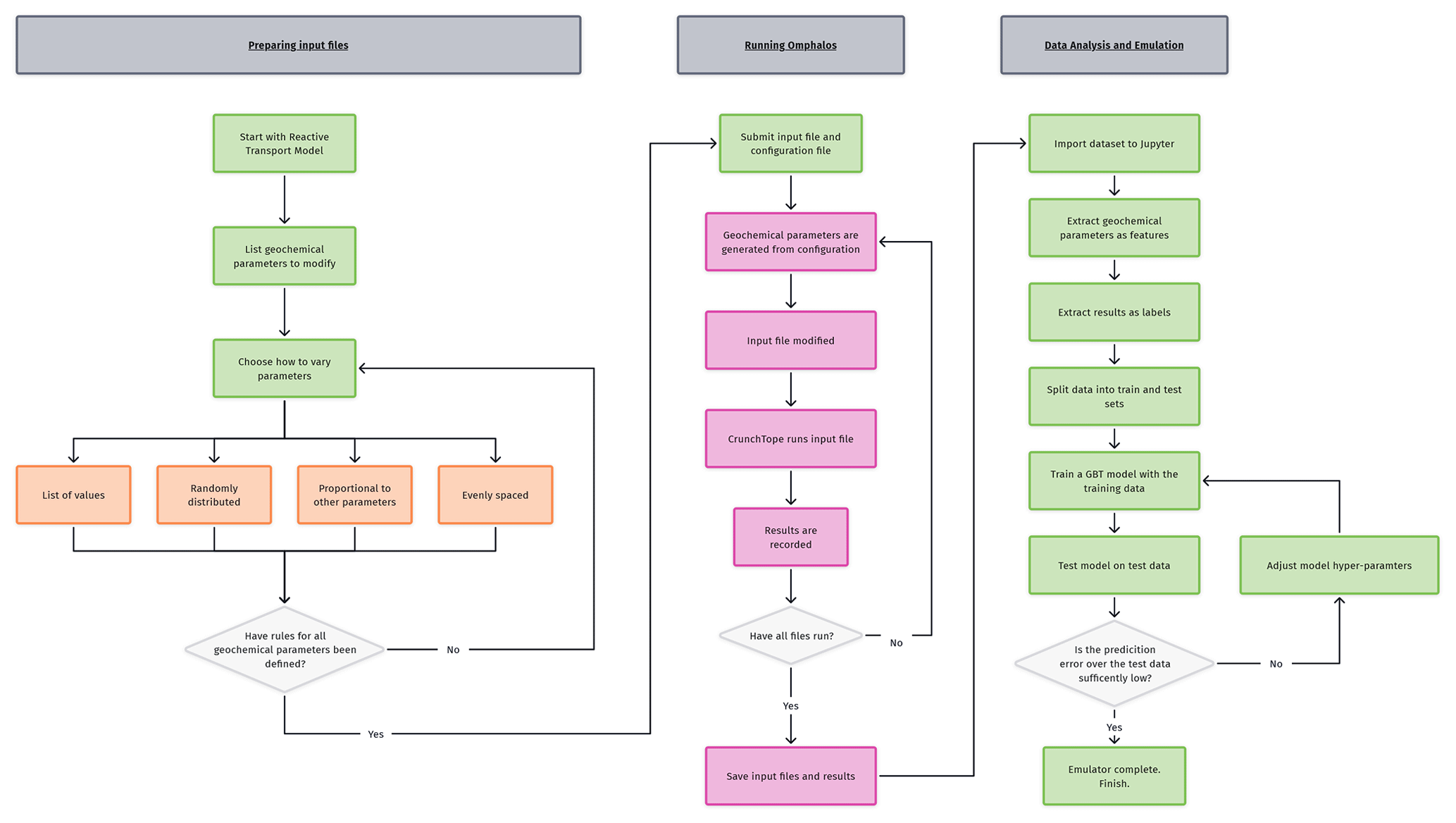
Figure 1 Flowchart describing the overall reactive transport emulation workflow developed in this study. It is divided into two key sections: (i) preparation of the input reactive transport model for submission to Omphalos and (ii) the analysis and emulation of the resultant data.

3 Methodology

3.1 General strategy

To explore the dependence of the RTM on the chosen environmental variables, we begin with a Monte Carlo approach; we draw random values for each parameter and record the model output under that randomised condition. We then fit a model to this Monte Carlo-generated dataset using a GBT regressor. This fitting results in a model (our emulator – RTE) that reproduces the complex interdependencies of chemical species that are encoded in the original, underlying RTM. This emulator can be interrogated to examine the dependence of the RTM outputs on the originally chosen environmental variables in an efficient, multivariate way. This way of performing sensitivity analyses has the potential to give insight into trends and relationships that would not be apparent otherwise and ultimately allows us to investigate the sensitivity of the model outputs with respect to the RTM's original parameterisation. First, we will describe how we use the Monte Carlo approach to generate data and then how we fit a model to this data. The overall workflow is shown in Fig. 1.

3.2 Generating data

We use the open-source software CrunchTope as the reactive transport framework for the models in this study. To generate the synthetic datasets necessary for our approach, and given the time-consuming nature of generating a single point (requiring a complete run of the RTM, along with modified boundary conditions), we developed a software package in Python to automate this process. This software package can manage the automatic generation and submission of unique input files to CrunchTope, as well as record the output of each run, storing it in a manageable data structure for future use. Use of the software package is straightforward, requiring the configuration of a single file listing which species and/or parameters are to be varied and how they should be varied.

We have named this software package Omphalos (available for download – Sect. 5.1). Omphalos can be run on clusters using Simple Linux Utility for Resource Management (Yoo et al., 2003) to execute input files in parallel or to run locally with CrunchTope simulations on individual CPUs, which considerably reduces the time required to generate large datasets. Omphalos works by taking random values which are drawn from uniform distributions (other statistical distributions are possible) of the chosen variables, sampling the space evenly. This provides a complete dataset for training the emulator.

While the underlying principle of training emulators on synthetic data can be applied to any reactive transport code, currently the software used to implement the approach is only compatible with CrunchTope because the input file reading and writing must be in a specific format. The approach is readily generalised, however, and the methodology could be applied to any RTM software (e.g. Geochemist's Workbench, TOUGHREACT), provided that the string input–output code is adapted for compatibility.

3.3 Application to contaminated-aquifer case study

We begin by applying the emulation methodology to our case study. To create the dataset for training the emulator, we collected the results of 10 927 unique CrunchTope simulations based on the original RTM describing Old Rifle using Omphalos, drawing random concentrations for five chosen species (${\mathrm{NH}}_{\mathrm{4}}^{+}$, ${\mathrm{SO}}_{\mathrm{4}}^{\mathrm{2}-}$, Ca²⁺, ${\mathrm{C}}_{\mathrm{2}}{\mathrm{H}}_{\mathrm{3}}{\mathrm{O}}_{\mathrm{2}}^{-}$, and pCO₂) in the boundary condition. Of these 10 927 runs, 9416 provide useable data because some runs fail to converge within the specified time frame, or the geochemical condition generated cannot be charge balanced. Excluding these runs helps ensure that our dataset is kept realistic because our RTM is built on a mechanistic understanding and implementation of the physical processes at work in the system that have been validated in some way. Therefore, runs that take excessively long to run fail to converge in the simulation scheme of CrunchTope and hence are likely to be unphysical in some way. Similarly, runs that fail to speciate or charge balance indicate some kind of extreme physical condition that is unlikely to be realistic, and so these are excluded. The concentrations for ${\mathrm{NH}}_{\mathrm{4}}^{+}$, ${\mathrm{SO}}_{\mathrm{4}}^{\mathrm{2}-}$, Ca²⁺, and ${\mathrm{C}}_{\mathrm{2}}{\mathrm{H}}_{\mathrm{3}}{\mathrm{O}}_{\mathrm{2}}^{-}$ are varied between 0–30 mM. The pCO₂ is varied between 0–10 bar. We acknowledge that these ranges of concentrations are somewhat higher than those that occur in natural systems, but we extend the range to observe RTM behaviours at limiting concentrations. Related to this, it is possible for the dominant reaction mechanism in a system to change under differing conditions (e.g. the change in the calcite dissolution mechanism as a function of pH; Dolgaleva et al., 2005), and any such behaviour should be explicitly encoded into the RTM, otherwise the emulator may give invalid predictions under conditions that are far from the original model run. We have assumed in this study that the mechanisms governing the precipitation of pyrite do not change under very low or very high concentrations of these species.

The injection fluid was constrained at pH 7.2. This constraint, in conjunction with the concentration of various species iterated in Omphalos, speciates according to CrunchTope's internal speciation calculation. Therefore, for example, although the total amount of ${\mathrm{SO}}_{\mathrm{4}}^{\mathrm{2}-}$ in the injection will be iterated in and dictated by Omphalos, the amount that speciates into other aqueous complexes (i.e. secondary species) like ${\mathrm{HSO}}_{\mathrm{4}}^{-}$ or H₂SO_4(aq) is controlled by CrunchTope. For the sake of simplicity, we will report the input concentration and not the concentration after speciation.

The RTM describing Old Rifle has 100 grid cells with a size of 1 cm. Each run of the RTM took approximately 90 s, so the total time to generate the dataset was roughly 4 h when run on a remote machine with 200 CPUs. The number of runs was chosen as a balance between what was computationally tractable and the ability of the emulator to achieve a good fit. We have intentionally chosen to vary some chemical species in the influent boundary condition that do not play an obvious role in the mineral precipitation process we are particularly interested in, namely, the precipitation of pyrite in Old Rifle sediments (e.g. ${\mathrm{NH}}_{\mathrm{4}}^{+}$ or Ca²⁺). We did this to see if we can use the emulator to detect behaviour in the RTM beyond what we might initially hypothesise.

3.4 Fitting the emulator

We implement the GBT regressor using XGBoost (Chen et al., 2016) in Python. The code for fitting the models is available in the Supplement. For a précise on GBT models, see the Sect. S1.2 in the Supplement.

3.4.1 Data strategy

Data generated by Omphalos were imported into a Jupyter Notebook environment from the .pkl output file. There are 9416 different input file runs in this data file, having excluded 1511 runs on the grounds of them being unrealistic, as discussed previously. The relevant data were indexed out of the data structure; in our case, this meant the concentrations of ${\mathrm{NH}}_{\mathrm{4}}^{+}$, ${\mathrm{SO}}_{\mathrm{4}}^{\mathrm{2}-}$, Ca²⁺, and ${\mathrm{C}}_{\mathrm{2}}{\mathrm{H}}_{\mathrm{3}}{\mathrm{O}}_{\mathrm{2}}^{-}$ in the boundary condition, as well as the value of pCO₂. This results in a 5 × 9416 array of floating-point numbers for the features. Each feature was then normalised to be in the range 0 to 1 for training. For example, values of the ${\mathrm{SO}}_{\mathrm{4}}^{\mathrm{2}-}$ concentration in the simulations were drawn randomly between 0 and 30 mM so all ${\mathrm{SO}}_{\mathrm{4}}^{\mathrm{2}-}$ concentrations were divided through by 30 to have values in the range 0–1. We did this to improve the training performance of the GBT model over different datasets (i.e. so that the same GBT model can be applied to both the Old Rifle case study and our supplementary case study of Ocean Drilling Program (ODP) Site 1086 (see Sect. S3 in the Supplement)).

Similarly, the relevant data were also extracted from the data file: for each cell in the gridded RTM, we calculated the net pyrite precipitation over the course of the simulation and then summed this value over the column to get the net pyrite precipitated across the domain. This results in a 1 × 9416 array of floating-point labels to be predicted from the feature array. We scale this feature array by a factor of 1 × 10⁴ to avoid issues with small floating-point numbers in XGBoost.

We prepared these data for training the GBT regressor with a hold-out strategy using the scikitlearn.train_test_split method, keeping 10 % of the dataset back for validating the model. Data were split randomly within the dataset. This means that 8474 randomly selected data points were used to train the model, and 942 randomly selected data points were used to test it by using the model to predict a value based on the held-back data and comparing the prediction to the true value.

3.4.2 Training strategy

We use the data points generated by Omphalos to train an XGBoost regressor using the squared error as the loss function to predict the amount of pyrite precipitated in the column as a function of varied species concentrations in the boundary condition. The squared log loss and pseudo-Huber error were also tried, but the squared loss performed best overall. Training curves showing the testing and training loss as training progressions are given in Fig. S2 in the Supplement.

Hyperparameter choices for the model are explained and given in Sect. S1.3, Table S1 in the Supplement. The choice of hyperparameters is the same for each emulator model, and we are able to achieve high-quality fits using the default XGBoost regularisations, only changing a few settings relating to tree growth policy. While it is a known problem in machine learning that the choice of optimal hyperparameter is dependent on the data being modelled (Claesen and De Moor, 2015), it appears that, in the context of these RTEs, the hyperparameters chosen give a good fit for both Old Rifle and our supplementary case study of ODP Site 1086 – datasets describing very different natural environments, with different length and timescales. This makes the workflow applicable across a wide variety of reactive transport modelling domains.

It is possible that with more complex hyperparameter tuning, better emulator fits may be achieved, but for the purposes outline in this paper, we suggest that this automated optimisation of a subset of the available hyperparameters is sufficient and represents a balance between emulator fit, generalisability across differing RTMs, and time spent by the user.

3.4.3 Model metrics

We report our model goodness of fit to the underlying dataset as the R² value for the model, using the built in XGBRegressor.score() method from XGBoost's scikit-learn API for both the original training dataset and the 10 % of the dataset held back for validation, as show in Table 1. We also report the root-mean-square error (RMSE) over both the training and validation datasets, calculated using the Booster.eval() method. Training curves are shown in Fig. S2. We report the same metrics for our second model in Table S4 in the Supplement.

Table 1 Training and validation metrics for the XGBoost regressor model fit to the Old Rifle dataset. R² represent a normalised measure of the fit quality, with the best possible score being 1. RMSE is the root-mean-squared error in the predictions, where we recall that, in data pre-processing, the values to be predicted were multiplied by a factor of 10⁴, and so the RMSE should be divided by that factor when assessing the average error for data presented in Figs. 2–4.

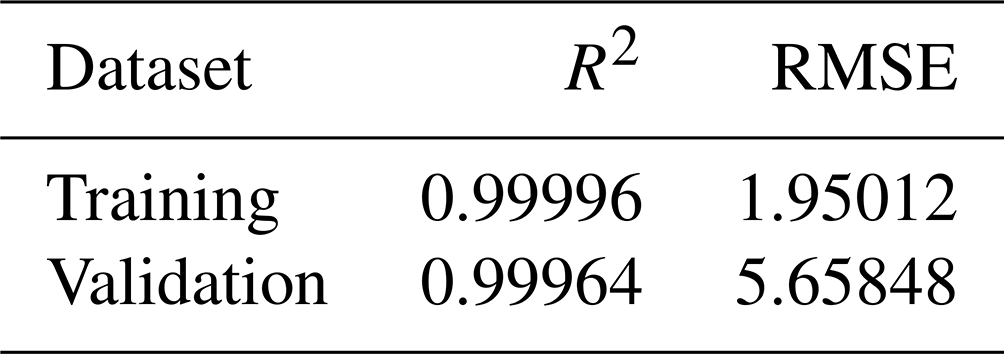
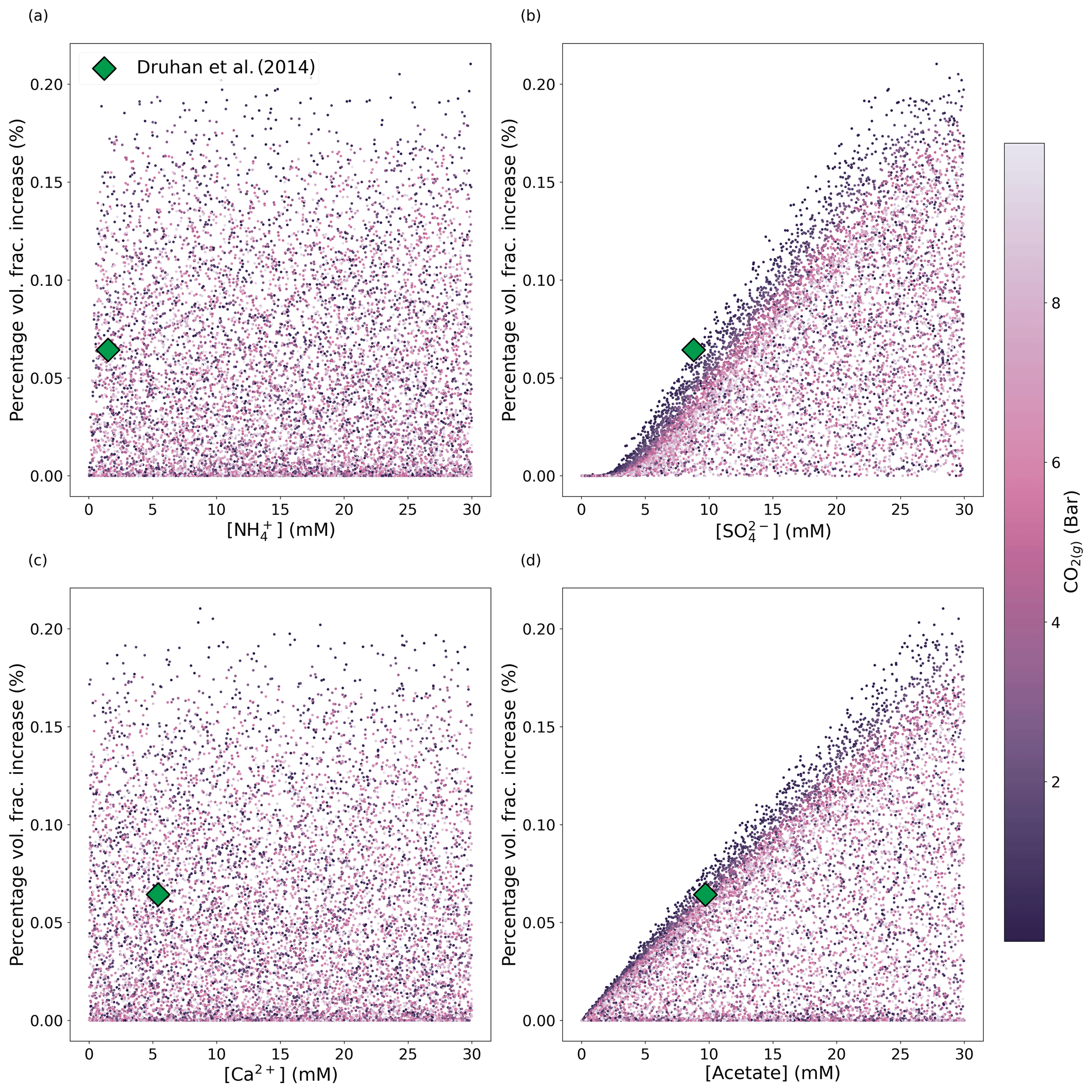
Figure 2 Scatterplots of chemical concentrations in the fluid injectate (influent boundary condition) for an RTM adapted to Old Rifle sediments colour mapped by the pCO₂ with which the inlet boundary condition is in equilibrium. The dataset comprises 9416 points generated by drawing concentrations for all five species independently from uniform random distributions, with the corresponding net increase in pyrite volume fraction precipitated (y axis) calculated by running the Old Rifle RTM designed by Druhan et al. (2014) with the randomised influent boundary condition. The green diamond indicates the net pyrite volume fraction generated from the original boundary condition used in Druhan et al. (2014).

4 Results and discussion

4.1 Application to the Old Rifle Site

The synthetic data generated using Omphalos to interrogate the underlying RTM are shown in Fig. 2, colour mapped by the pCO₂ with which the injectate solution is in equilibrium. The colour mapping helps visualise how variability in the precipitated volume of pyrite over the 43 d RTM simulation might be considered in conjunction with other model parameters. Ultimately, pyrite forms because aqueous hydrogen sulfide, produced through microbial sulfate reduction, reacts with reduced ferrous iron (Fe(II)) to form pyrite. Thus, we aim to explore the interdependencies between the mechanisms driving microbial sulfate reduction and the subsequent precipitation of pyrite as they emerge due to variations in injectate chemical composition.

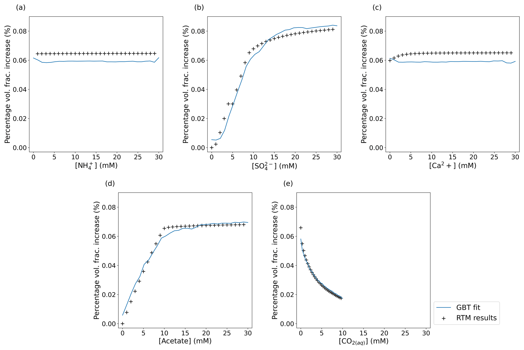
Figure 3 Plots of the GBT model fit (blue line) plotted over the results from the underlying RTM (black + symbols) when interrogated with the same input parameters (which are taken as ground truth). Each plot shows the net volume fraction due to pyrite precipitation as a percentage of the initial volume fraction of the sediment as each parameter is varied while all other parameters are held at the values used in the original experiment by Druhan et al. (2014). The emulator (blue line) captures the overall trends in the data. The lack of smoothness in the emulator predications arises from the inability to encode this as a condition in XGBoost and the discreet nature of the decision tree algorithm. The RTM results compared to here are not part of the training dataset, and so the emulator has not been exposed to those exact values.

We then train the emulator on this synthetic dataset. Fitting a GBT regressor to the data in Fig. 2 means Fig. 3 can be generated by the emulator. This figure shows how the emulator predicts the change in pyrite volume fraction as the concentration of each of the species in the injection fluid is varied (other species in the RTM not defined as variables in this study are held constant at values reported by Druhan et al., 2014). We stress that the RTM results shown in Fig. 3 are not part of the training dataset and that the emulator has not been exposed to these exact values. This demonstrates the capability of the emulator to reproduce the underlying RTM itself. For example, Fig. 2a suggests visually that the concentration of ${\mathrm{NH}}_{\mathrm{4}}^{+}$ in the system is uncorrelated with net pyrite precipitation at the Old Rifle site. Figure 3a confirms this lack of dependence on ${\mathrm{NH}}_{\mathrm{4}}^{+}$, capturing the correct trend (with some noise), although it is slightly offset. This slight offset also applies to Fig. 3c in the fit of the Ca²⁺ dependence. We suggest that these slight offsets to the fits in the cases of the weakly or uncorrelated variables are due to the emulator preferentially capturing stronger dependencies and slightly drawing down the predicated variable on average.

In contrast to the minimal impact that changing ${\mathrm{NH}}_{\mathrm{4}}^{+}$ concentration has on pyrite precipitation, ${\mathrm{C}}_{\mathrm{2}}{\mathrm{H}}_{\mathrm{3}}{\mathrm{O}}_{\mathrm{2}}^{-}$ and ${\mathrm{SO}}_{\mathrm{4}}^{\mathrm{2}-}$ concentrations correlate strongly with net pyrite precipitation. This is as expected in a system where ${\mathrm{C}}_{\mathrm{2}}{\mathrm{H}}_{\mathrm{3}}{\mathrm{O}}_{\mathrm{2}}^{-}$, which is the electron donor for microbial sulfate reduction, enables sulfate to be reduced to sulfide and thus drives pyrite precipitation in the presence of Fe(II). Approximately 20 d after ${\mathrm{C}}_{\mathrm{2}}{\mathrm{H}}_{\mathrm{3}}{\mathrm{O}}_{\mathrm{2}}^{-}$ amendment, microbial sulfate reduction takes over from dissimilatory iron reduction as the dominant process consuming ${\mathrm{C}}_{\mathrm{2}}{\mathrm{H}}_{\mathrm{3}}{\mathrm{O}}_{\mathrm{2}}^{-}$. As microbial sulfate reduction requires 8 times the number of electrons per mole of ${\mathrm{SO}}_{\mathrm{4}}^{\mathrm{2}-}$ reduced than dissimilatory iron reduction requires (per mole of iron reduced), the electron donor (${\mathrm{C}}_{\mathrm{2}}{\mathrm{H}}_{\mathrm{3}}{\mathrm{O}}_{\mathrm{2}}^{-}$) begins to be rapidly consumed, whereas during dissimilatory iron reduction, it was effectively in excess. As a result of this new scarcity of ${\mathrm{C}}_{\mathrm{2}}{\mathrm{H}}_{\mathrm{3}}{\mathrm{O}}_{\mathrm{2}}^{-}$, the rate of dissimilatory iron reduction drops, and so does the concentration of Fe(II). However, dissimilatory iron reduction is still active in the column, releasing a small – but non-zero – flux of aqueous Fe(II) that allows for continued pyrite precipitation. The emulator interprets this as Fe(II) being always available in this system and thus predicts that pyrite precipitation can scale linearly with ${\mathrm{SO}}_{\mathrm{4}}^{\mathrm{2}-}$ and ${\mathrm{C}}_{\mathrm{2}}{\mathrm{H}}_{\mathrm{3}}{\mathrm{O}}_{\mathrm{2}}^{-}$, as shown in Fig, 4a. The sediment itself would need to contain abundant ferrihydrite, goethite, or another bioavailable ferri(hydr)oxide for this reduction to continue indefinitely; this may not be the case. This highlights the need for the range of parameters sampled when training the emulator to be sufficiently wide to capture all the RTM behaviour, otherwise it may extrapolate and learn incorrect assumptions about the system – in this case, that bioavailable iron never limits dissimilatory iron reduction. One solution would be to expand the range over which concentrations are drawn to reach the limit where the iron-bearing mineral volume fraction becomes a limiting factor so that the model can learn what happens when this occurs.

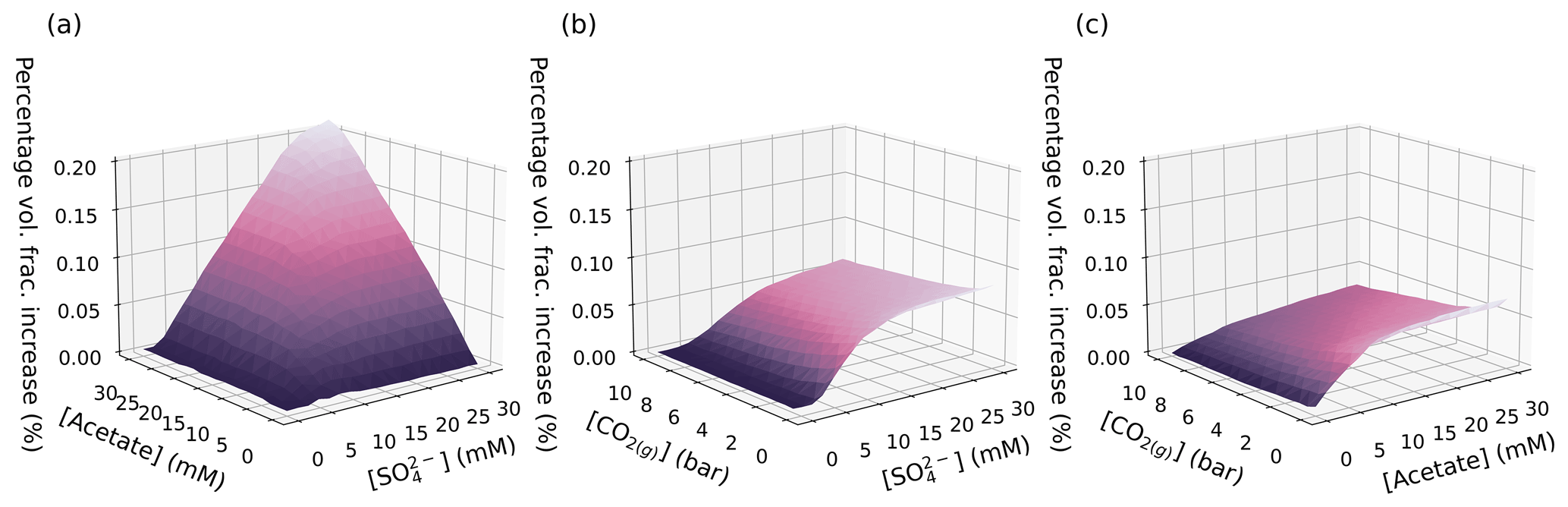
Figure 4 A selection of the GBT model predictions of the percentage volume fraction increase due to pyrite precipitation as a result of varying two parameters simultaneously for selected pairs of variables. Other model parameters are held at the values used in Druhan et al. (2014). The remaining variable-pair plots are provided in Fig. S4.

We also note that our emulator suggests that increasing pCO₂ leads to decreased pyrite precipitation (Fig. 3e), a relationship that may not have been apparent in a single run of the RTM. Three-dimensional visualisation of the data confirms that the pyrite volume fraction change varies as a function of pCO₂ net pyrite precipitated decreasing as pCO₂ increases (Fig. 4b and c). This three-dimensional visualisation allows us to see that the gradient of the pyrite volume fraction change with respect to ${\mathrm{SO}}_{\mathrm{4}}^{\mathrm{2}-}$ and ${\mathrm{C}}_{\mathrm{2}}{\mathrm{H}}_{\mathrm{3}}{\mathrm{O}}_{\mathrm{2}}^{-}$ is itself a function of pCO₂ and flattens as pCO₂ increases. To understand why the gradient changes, we must first understand why pCO₂ affects the amount of pyrite precipitated in the first place.

Sediment samples from Old Rifle are initially poised for dissimilatory iron reduction, and there is a sizeable community of iron-reducing bacteria naturally present in the system. The background sulfate-reducing microbial community is initially relatively small, and thus, for microbial sulfate reduction to proceed at significant rates, the mass of sulfate-reducing bacteria must first increase. In the original experiment by Druhan et al. (2014), the sulfate-reducing biomass begins to reach a size where it can start consuming large quantities of ${\mathrm{C}}_{\mathrm{2}}{\mathrm{H}}_{\mathrm{3}}{\mathrm{O}}_{\mathrm{2}}^{-}$ around day 20 of the experiment. This biomass growth is modelled in CrunchTope using a Monod biomass rate law (Jin and Bethke, 2005), which has both an anabolic and a catabolic component. In the formulation of this Monod biomass rate law, as implemented in CrunchTope, the thermodynamic term (Gibbs free energy of the reaction) is calculated exclusively using the catabolic pathway. The catabolic pathway for this reaction (in terms of the exchange of one electron) is given below in Eq. (1), and the form of the Gibbs free energy is this context is given in Eq. (2) (we take the phosphorylation potential to be 0 and the average stoichiometric number to be 1; see derivation in Jin and Bethke (2005) for further details).

$$\begin{array}{}\text{(1)}& {\displaystyle }\begin{array}{rl}{\displaystyle \frac{\mathrm{1}}{\mathrm{8}}}{\mathrm{SO}}_{\mathrm{4}}^{\mathrm{2}-}& +{\displaystyle \frac{\mathrm{1}}{\mathrm{8}}}{\mathrm{C}}_{\mathrm{2}}{\mathrm{H}}_{\mathrm{3}}{\mathrm{O}}_{\mathrm{2}}^{-}+{\displaystyle \frac{\mathrm{3}}{\mathrm{8}}}{\mathrm{H}}^{+}\to {\displaystyle \frac{\mathrm{1}}{\mathrm{8}}}{\mathrm{H}}_{\mathrm{2}}{\mathrm{S}}_{\left(\mathrm{aq}\right)}+{\displaystyle \frac{\mathrm{1}}{\mathrm{4}}}{\mathrm{CO}}_{\mathrm{2}\left(\mathrm{aq}\right)}\\ & +{\displaystyle \frac{\mathrm{1}}{\mathrm{4}}}{\mathrm{H}}_{\mathrm{2}}\mathrm{O}\end{array}\text{(2)}& {\displaystyle }\mathrm{\Delta }G=\mathcal{R}\mathcal{T}\ln \left({\displaystyle \frac{\left[{\mathrm{CO}}_{\mathrm{2}\left(\mathrm{aq}\right)}{]}^{\frac{\mathrm{1}}{\mathrm{4}}}\right[{\mathrm{H}}_{\mathrm{2}}{\mathrm{S}}_{\left(\mathrm{aq}\right)}{]}^{\frac{\mathrm{1}}{\mathrm{8}}}}{\left[{\mathrm{SO}}_{\mathrm{4}}^{\mathrm{2}-}{]}^{\frac{\mathrm{1}}{\mathrm{8}}}\right[{\mathrm{C}}_{\mathrm{2}}{\mathrm{H}}_{\mathrm{3}}{\mathrm{O}}_{\mathrm{2}}^{-}{]}^{\frac{\mathrm{1}}{\mathrm{8}}}[{\mathrm{H}}^{+}{]}^{\frac{\mathrm{3}}{\mathrm{8}}}}}\right)\end{array}$$

Taking this form for the Gibbs free energy of the reaction and substituting it into the thermodynamic term of the reaction rate calculation as implemented in CrunchTope (Steefel et al., 2015) gives Eq. (3) below, describing the rate of microbial sulfate reduction in the Rifle RTM:

$$\begin{array}{}\text{(3)}& \begin{array}{rl}{R}_{\text{MB}}=& k_{\text{max}}B{\displaystyle \frac{\left[{\mathrm{C}}_{\mathrm{2}}{\mathrm{H}}_{\mathrm{3}}{\mathrm{O}}_{\mathrm{2}}^{-}\right]}{\left[{\mathrm{C}}_{\mathrm{2}}{\mathrm{H}}_{\mathrm{3}}{\mathrm{O}}_{\mathrm{2}}^{-}\right]+K_{\text{half}\left[\text{Ace}\right]}}}\\ & \times {\displaystyle \frac{\left[{\mathrm{SO}}_{\mathrm{4}}^{\mathrm{2}-}\right]}{\left[{\mathrm{SO}}_{\mathrm{4}}^{\mathrm{2}-}\right]+K_{\text{half}\left[{\mathrm{SO}}_{\mathrm{4}}^{\mathrm{2}-}\right]}}}{F}_{\mathrm{T}},\end{array}\end{array}$$

where

$$\begin{array}{}\text{(4)}& F_{\mathrm{T}}=\left(\mathrm{1}-{\displaystyle \frac{\left[{\mathrm{CO}}_{\mathrm{2}\left(\mathrm{aq}\right)}{]}^{\frac{\mathrm{1}}{\mathrm{4}}}\right[{\mathrm{H}}_{\mathrm{2}}{\mathrm{S}}_{\left(\mathrm{aq}\right)}{]}^{\frac{\mathrm{1}}{\mathrm{8}}}}{\left[{\mathrm{SO}}_{\mathrm{4}}^{\mathrm{2}-}{]}^{\frac{\mathrm{1}}{\mathrm{8}}}\right[{\mathrm{C}}_{\mathrm{2}}{\mathrm{H}}_{\mathrm{3}}{\mathrm{O}}_{\mathrm{2}}^{-}{]}^{\frac{\mathrm{1}}{\mathrm{8}}}[{\mathrm{H}}^{+}{]}^{\frac{\mathrm{3}}{\mathrm{8}}}}}\right).\end{array}$$

R_MB is the overall rate of microbial sulfate reduction, k_max is the rate constant for microbial sulfate reduction, B is the biomass concentration, and K_half[X] is a half-saturation constant. The two Monod kinetic factors for the electron donor (${\mathrm{C}}_{\mathrm{2}}{\mathrm{H}}_{\mathrm{3}}{\mathrm{O}}_{\mathrm{2}}^{-}$) and the electron acceptor (${\mathrm{SO}}_{\mathrm{4}}^{\mathrm{2}-}$) are referred to as F_D and F_A, respectively (Jin and Bethke, 2003, 2005, 2007). Equation (4) illustrates the underlying relationship between pCO₂ in the injectate solution and the resulting accumulation of pyrite. As the pCO₂ of the injectate increases, the F_T term becomes smaller, inhibiting the overall rate of microbial sulfate reduction (Fig. S5). Consequently, biomass growth is also inhibited, and the rate of microbial sulfate reduction is never high enough to produce the concentration of H₂S_(aq) required for significant pyrite precipitation. This explains why the model suggests that the gradient of the pyrite volume precipitated with respect to both ${\mathrm{C}}_{\mathrm{2}}{\mathrm{H}}_{\mathrm{3}}{\mathrm{O}}_{\mathrm{2}}^{-}$ and ${\mathrm{SO}}_{\mathrm{4}}^{\mathrm{2}-}$ varies as a function of pCO₂ in the injectate. When pCO₂ is low and both ${\mathrm{SO}}_{\mathrm{4}}^{\mathrm{2}-}$ and ${\mathrm{C}}_{\mathrm{2}}{\mathrm{H}}_{\mathrm{3}}{\mathrm{O}}_{\mathrm{2}}^{-}$ are large with respect to their half-saturation constants (Eq. 4), the overall Monod biomass rate law will approach Bk_max.

This dependence emerged somewhat unexpectedly from the emulator as one would not inherently expect a relationship between injectate pCO₂ and ${\mathrm{SO}}_{\mathrm{4}}^{\mathrm{2}-}$ reduction rates, yet it agrees with results previously reported by Jin and Kirk (2016, 2018), as well as by Paper et al. (2021). These studies related the influence of pCO₂ and pH to the rate of microbial reactions in vitro, in situ, and in silico. We suggest that our type of analysis could be used to direct future lab and field work to test hypotheses suggested by the results generated by running the emulator.

This analysis also explains some of the features observed in Fig. 4a: the gradients of ${\mathrm{C}}_{\mathrm{2}}{\mathrm{H}}_{\mathrm{3}}{\mathrm{O}}_{\mathrm{2}}^{-}$ and ${\mathrm{SO}}_{\mathrm{4}}^{\mathrm{2}-}$ are coupled in such a way as to indicate that if one is in excess, then the other becomes limiting in the production of H₂S_(aq) and hence the precipitation of pyrite. However, the limiting behaviour when both are in excess seems to indicate that, given enough ${\mathrm{SO}}_{\mathrm{4}}^{\mathrm{2}-}$ and ${\mathrm{C}}_{\mathrm{2}}{\mathrm{H}}_{\mathrm{3}}{\mathrm{O}}_{\mathrm{2}}^{-}$, pyrite precipitation can continue indefinitely assuming suitably low pCO₂. Given this prediction, it is sensible to check whether, at such high levels of ${\mathrm{SO}}_{\mathrm{4}}^{\mathrm{2}-}$ and ${\mathrm{C}}_{\mathrm{2}}{\mathrm{H}}_{\mathrm{3}}{\mathrm{O}}_{\mathrm{2}}^{-}$, as the model suggests for maximum pyrite precipitation, there is indeed enough Fe(II) available in the system to precipitate pyrite; this is a second potential dependence, as mentioned above.

Lastly, the model can be interrogated in all five dimensions, and the amendment fluid composition that corresponds to the largest net pyrite precipitation over the modelled interval can be determined. We do this simple optimisation by evaluating the emulator at regular intervals across all five dimensions at intervals of ∼ 2 mM (intervals of ∼ 0.67 mM for pCO₂) in the range that the emulator was trained on (0–30 mM, except for pCO₂, which has a range of 0–10 mM). This corresponds to checking 759 375 different boundary conditions to find which boundary condition results in the most net pyrite precipitation and takes ∼ 7 min. This amendment composition is shown in Table S1. The total change in volume fraction due to pyrite precipitation predicted by the emulator is 0.143, and the actual RTM-modelled precipitation when this boundary condition is used is 0.150. There is a 4.7 % absolute error for the net pyrite volume fraction change predicted by the emulator when compared to the actual net pyrite precipitation calculated by the RTM. This error is inherent in statistical learning techniques but can be further mitigated with larger training datasets in conjunction with different emulator-training hyperparameterisations, an area for future improvement to the methodology. These optimised conditions represent an almost 4-fold increase in the amount of pyrite precipitated in the original RTM for Old Rifle (Druhan et al., 2014).

4.2 Advantages and drawbacks of the emulation approach

In this study, 9416 individual RTM simulations were used to train a GBT regression model to predict a specific model output, in this case net pyrite precipitation. This emulator is a reduced representation of the complex system of equations in the underlying RTM, having a faster computational time but introducing some prediction errors. We now discuss the key advantages and drawbacks of this emulation approach.

4.3 Advantages of the emulation approach

A total of 9416 RTM runs were used to train the emulator (the data shown in Fig. 2). This number of runs could instead be used to perform a sensitivity analysis of all five variables at a spacing of ∼ 4.8 mM between points by directly interrogating the simulator. What then is the advantage of the emulation approach if the same information can be visualised from discreet runs of the original RTM without having to exert the extra effort to train the model, which introduces prediction errors? The key advantages are outlined below.

4.3.1 Advantages over directly interrogating the simulator

The first and most obvious advantage is the lack of a need for an explicit interpolation scheme. Correlations generated by directly plotting simulator results lead to data points lying on a grid of finite resolution. If intermediate values on this grid were to be determined, an explicit interpolation scheme would have to be applied, which would introduce its own errors that would then need to be quantified. Furthermore, an improvement in the interpolation scheme would come at the expense of adding one extra point to the grid in each dimension; in the context of Old Rifle, this is an extra 9031 data points (${\mathrm{7}}^{\mathrm{5}}-{\mathrm{6}}^{\mathrm{5}}=\mathrm{9031}$ going from six points in all directions to seven on a 5D grid, roughly doubling the dataset size. In contrast, since any number of points can be submitted to the emulator for inference, concerns relating dataset size to sampling resolution are assuaged. Beyond that, the errors in the model fit are already quantified during training.

More broadly, to explore the data space, emulators are extremely fast compared to simulators. The time for a single query of the emulator is on the order of milliseconds rather than the seconds, minutes, or hours for a single forward RTM simulation. This allows the emulator to be used as a tool for efficiently exploring the simulator by rapidly developing an intuition for the space itself and how the simulator behaves in different circumstances. Furthermore, emulator models are easy to distribute and share with collaborators. Model weights can be published directly or distributed as standalone files. This means that a well-trained emulator can be made once, and then the encoded data can be shared.

Lastly, performing a direct interrogation of the simulator requires choices of parameters and ranges and results in a grid of points over the region of interest at limited resolution. A similar procedure must be undertaken when creating a dataset to train the emulator in so far as ranges and parameters of interest must be chosen. However, the dataset can always be further added to in a straightforward manner, further drawing from the random distribution to increase the size of the dataset and thus improve model performance. With both approaches, using Omphalos means that the data generation process can be parallelised, and using high-performance computing facilities can reduce the computational expense of interrogating the simulator. This means that all the computational expense is upfront in both cases since the emulator need only be fitted once.

The advantages we outline make the case for the emulator as a tool to be used in conjunction with the RTM rather than as a replacement for it. The alacrity with which the emulator can be interrogated means that it is an invaluable tool for investigating RTM behaviour in multiple dimensions. Further to this, the ability to evaluate the state of a system after a fixed period of time makes the emulator approach ideally suited for modelling more complex time series models with time-varying boundary conditions; instead of having to run the RTM forward each time the system changes boundary conditions, the emulator can be interrogated for the expected result given the system's current state from the previous regime.

4.3.2 Using emulators to identify new feedbacks

As modern RTMs grow in sophistication and complexity, they increasingly draw on large suites of chemical and mineralogical information from vast databases, which constitute large sets of non-linear equations all coupled through transport and fluid chemistry. While it is true that, for a sufficiently simple model, coupled geochemical behaviour could be deduced by reasoning about the governing equation of the systems, for a large, modern RTM it is inevitable that, during development, some feedbacks will be overlooked.

Emulation makes sensitivity analysis for RTMs simple and allows us to identify correlations and interactions among parameters that would otherwise be difficult to anticipate by allowing an investigator to quickly test a wide variety of hypotheses. We demonstrate this in the case of Old Rifle by identifying the CO₂ dependency of microbially mediated reactions (Bethke et al., 2011; Jin and Kirk, 2016, 2018; Paper et al., 2021). This ability to elucidate unexpected but key model dependencies and sensitivities could prove to be invaluable in helping direct RTM development.

4.3.3 Application to Bayesian optimisation

A critical advantage of the technique proposed here is that emulation is an essential part of Bayesian optimisation. Bayesian optimisation is an approach for finding global maxima and minima in systems whose objective functions are expensive to evaluate and do not return the gradients of that function (of which RTMs are an example) (Frazier, 2018). Bayesian optimisation works by applying an acquisition function that calculates the point that will give the most information about the function that requires optimisation. An emulator is then fit using these data points selected by the acquisition function, and the emulator is updated with a new point with each iteration. In this way, the optimiser balances the exploitation of known optima and the exploration of unevaluated regions of the function. Such an approach can find the global maximum with relatively few evaluations of the RTM.

This study lays the groundwork for future applications of Bayesian optimisation to highly dimensioned RTMs, potentially allowing for effective optimisation over many different (20 or more) parameters at once. By demonstrating that broad (but local) fits to the RTM with an emulator are possible, we have demonstrated that a GBT regressor can be used as an emulator informing a Bayesian optimisation algorithm in this context. This allows for a constellation of local fits in a highly dimensioned space as the algorithm searches for the global optimum in problems that would otherwise be computationally intractable. Bayesian optimisation could even be applied, with a suitable loss function, to optimise for multiple objectives at once (subject to trade-offs among objectives).

4.4 Disadvantages of the emulation approach

This emulation approach relies on the relative computational inexpensiveness of the RTM. In situations where the underlying model is expensive or time consuming to evaluate and where computational resources are limited, this modelling approach becomes unfeasible. However, this issue of computational expense can be allayed by the parallelised generation of data alluded to earlier, and only the most expensive RTMs would be intractable for a full emulator fit if this technique was deployed correctly, and even in this extreme case, Bayesian optimisation would still be possible.

Additionally, caution is needed when choosing the ranges over which the parameters will be drawn from the uniform random distributions. Key considerations include the number of points being generated relative to the size of the space being covered – a denser cluster of training data will result in a tighter fit at the expense of range. Conversely, with too small of a range, the emulator will not capture key behaviour or will be unable to learn about simulator edge cases, as discussed above with respect to the bioavailable iron in the Old Rifle RTM.

4.5 Choice of learning algorithm

Gradient-boosted trees outperformed other machine learning methods that we tested while building the emulators, such as Gaussian process regression. The downsides of GBT include the lack of ability to encode smoothness to preclude sharp discontinuities in the concentration–precipitation space or other such prior assumptions. Furthermore, a low root-mean-squared error over the entire model fit region does not necessarily imply a good fit globally; it may be that there are some regions of good fit and other regions of poor fit which make up an acceptable root-mean-square error over the whole space.

4.6 The effect of scale on emulator predictions

Our case study relies on the capacity of CrunchTope to predict changes in mineral volume fraction. Therefore, the errors in the predictions, and hence the utility of the approach, ultimately depend on the scale of the system being modelled and thus the sensitivity to what could be very small changes in mineral volume fraction.

When analysing the emulator to investigate how different processes in the underlying RTM affect each other, we are primarily considering an issue of whether the emulator can correctly learn the underlying model behaviour. We are also considering whether the emulator can capture the behaviour in the output variables with respect to a changing subset of RTM parameters (some of which we may not have expected at the outset). In this use case, the emulator is largely concerned with trends and gradients; Figs. 3, 4, S4, S8, and S9 show that this is accurately reported in all case studies. Comparing the case study considered in this paper to the additional case study presented in the Supplement, we see that they are discretised at different scales (2 m and 1 cm for the deep-sea sediment column and Old Rifle, respectively). However, the emulator for each RTM has root-mean-squared error overs the dataset (and hence absolute errors in prediction) that are of the same order of magnitude. This implies that the error in the absolute volume precipitated that each model predicts is different. However, the analysis of the trends and interactions emerging from both RTMs is equally valid in both cases.

When concerned with the optimisation capabilities of the emulator, the absolute value of the optimised quantity and, hence, the model scale must be considered. In large-scale systems, such as weathering of the critical zone, the error in the volume fraction change (5.5 × 10⁻⁵ for pyrite) is below the resolution of measurement techniques for mineral abundance (e.g. X-ray diffraction, XRD, and scanning electron microscopy, SEM; Gu et al., 2020). However, in smaller-scale systems where the microscale environment becomes increasingly important, these errors in volume fraction become much harder to ignore. For example, in the RTM experiments exploring the effects of scale on simulating mineral dissolution in porous media described by Jung and Navarre-Sitchler (2018), significant errors in changes in predicted volume fraction would propagate into calculated dissolution and/or precipitation rates, losing sensitivity in the results.

4.7 Extension to multiple outputs

Multiple output regression (the prediction of a vector of outputs rather than a single label) is experimentally available in XGBoost and supported by other machine learning implementations that we explored, including GPflow for Gaussian process regression. Given that our approach is currently limited to the prediction of one label per emulator trained, the availability of regressors that can predict more than one label off the shelf will greatly improve the utility of reactive transport emulation. The prediction of multiple outputs simultaneously will expand the scope of analysis to investigate the interaction of modelled processes in multiple outputs at once. In the context of optimisation problems, one possible application of an emulator like this could be to maximise mineral precipitation in one region of a system while trying to maximise dissolution in another region.

4.8 Improvements to the model

This proof-of-concept model demonstrates the fitting of an emulator over a relatively small range of environmental parameters. Future work will involve expanding the scope of the emulators both in terms of the number of parameters being varied and the range over which they are varied so that the entirety of the behaviour of the underlying model can be captured with more accuracy. There is also scope for adding time dependency to the GBT modelling approach to predict a time series of intermediate RTM states during the evolution of geochemical systems.

4.9 Potential applications

Our emulator approach is flexible; any quantity recorded by an RTM can be used as a target variable, and so the behaviour of any RTM output can be explored in detail to evaluate the model formulation. The behaviour of the system in response to the variation of any parameter under any other set of conditions can be projected out of the model and plotted in a straightforward manner. This approach can be extended to two or even three dimensions and time series thereof, and ultimately, the emulator can be interrogated for local maxima and minima to solve optimisation problems. This approach has potential applications in industry and in environmental remediation where the chemical composition of amendments can be predicted using an underlying reactive transport simulation, provided that that system is well understood.

Omphalos also has utility outside of generating datasets for emulation; its automated submission of CrunchTope input files means it can be used to systematically explore sets of input variables in an easy way simply by editing the Omphalos configuration file.

5 Conclusions

We have presented an emulator-based approach for interrogating and understanding multi-component RTMs. By building an emulator of an RTM that captures the multidimensional nature of the underlying model, we have demonstrated that such an approach can be used as a tool for performing global sensitivity analyses on RTMs. This allows us to investigate behaviour arising from the interaction among the many disparate processes that comprise RTMs. For example, we investigated how the Monod biomass parameterisation of microbial sulfate reduction interacted with the mechanism of pyrite precipitation. In this example, pyrite precipitation was inhibited when there was an excess of CO₂ in the column because the catabolic pathway was partially dependent on CO₂ concentration. This prevented the growth of sulfate-reducing biomass, ultimately curtailing the production of hydrogen sulfide required for pyrite precipitation. This behaviour reproduced results previously reported by Jin and Kirk (2016, 2018) and suggests that emulation approaches have utility in discovering unexpected but nonetheless real model behaviours, potentially directing future lab and field work.

The methodology we have laid out is flexible; any quantity recorded by an RTM can be used as a target variable, and so the behaviour of any RTM output can be explored in detail to evaluate the model formulation. The behaviour of the system in response to the variation of any parameter under any other set of conditions can be projected out of the model and plot in a straightforward manner. Emulator approaches can be extended to two or even three dimensions, and ultimately, the emulator can be interrogated for local maxima and minima to solve optimisation problems. We suggest that emulator-based approaches to exploring RTMs have potential applications in industry and in environmental remediation, where the chemical composition of amendments can be predicted using an underlying reactive transport simulation, provided that that system is well understood. The application of this optimisation process to Old Rifle (and to ODP Site 1086; see the Supplement) represents a proof of concept.