Monte Carlo drift correction – quantifying the drift uncertainty of global climate models

Global climate models are susceptible to drift, causing spurious trends in output variables. Drift is often corrected using data from a control simulation. However, internal climate variability within the control simulation introduces uncertainty to the drift correction process. To quantify this drift uncertainty, we develop a probabilistic technique: Monte Carlo drift correction (MCDC). MCDC samples the standard error associated with drift in the control time series. We apply MCDC to an ensemble of global climate models from the Coupled Model Intercomparison Project Phase 6 (CMIP6). We find that drift correction partially addresses a problem related to drift: energy leakage. Nevertheless, the energy balance of several models remains suspect. We quantify the drift uncertainty of global quantities associated with the Earth's energy balance and thermal expansion of the ocean. When correcting drift in a cumulatively integrated energy flux, we find that it is preferable to integrate the flux before correcting the drift: an alternative method would be to correct the bias before integrating the flux, but this alternative method amplifies the drift uncertainty. Assuming that drift is linear likely leads to an underestimation of drift uncertainty. Time series with weak trends may be especially susceptible to drift uncertainty: for historical thermosteric sea level rise since the 1850s, the drift uncertainty can range from 3 to 24 mm, which is of comparable magnitude to the impact of omitting volcanic forcing in control simulations. Derived coefficients – such as the ocean's expansion efficiency of heat – can also be susceptible to drift uncertainty. When evaluating and analysing global climate model data that are susceptible to drift, researchers should consider drift uncertainty.

1 Introduction

Global climate models are susceptible to drift (Sen Gupta et al., 2013; Irving et al., 2021), causing spurious trends in output variables such as thermosteric sea level rise. Drift may also influence derived climate indices (Sanderson, 2020). Drift is not caused by transient external forcing (Sen Gupta et al., 2013). Instead, drift in long-term centennial-scale simulations is caused by two primary factors: insufficient spin-up and model errors (Hobbs et al., 2016).

First, drift may occur due to insufficient spin-up of equilibrium simulations (Sen Gupta et al., 2013; Hobbs et al., 2016). Following a perturbation to equilibrium forcing, the deep ocean responds slowly, taking millennia to approach a quasi-equilibrium state (Stouffer, 2004; Stouffer et al., 2004; Eyring et al., 2016). Therefore, variables influenced by the deep ocean are especially susceptible to drift (Sen Gupta et al., 2013). The slow response of the deep ocean is consistent with the physics of the real climate system. This source of drift can be reduced by increasing the spin-up length of equilibrium simulations.

Second, drift may arise due to errors – including biases – in the climate model (Hobbs et al., 2016; Brunetti and Vérard, 2018; Irving et al., 2021). Even when climate models are spun up for long periods under equilibrium forcing, modelled variables may be inconsistent with a true quasi-equilibrium state – spurious trends remain (Hobbs et al., 2016). Of particular relevance here is the problem of energy leakage (Irving et al., 2021): unphysical sinks and sources of energy contribute to inconsistent biases in the top-of-atmosphere radiative flux and the sea surface heat flux (Sect. 4.1; Lucarini and Ragone, 2011; Hobbs et al., 2016). Such biases indicate defects in the tuning procedure and the parameterisations included in the global climate model (Brunetti and Vérard, 2018).

Fortunately, drift can often be corrected when analysing global climate model data (Sen Gupta et al., 2013). Correcting drift may also address the problem of energy leakage (Hobbs et al., 2016; Irving et al., 2021). Most drift correction methods rely on control simulations (Sen Gupta et al., 2013). These control simulations are forced by equilibrium forcing consistent with pre-industrial conditions using 1850 as the reference year (Eyring et al., 2016). Such control simulations provide initial conditions for historical simulations.

A commonly used drift correction method involves fitting a linear trend to the entire control time series of a state variable (Sen Gupta et al., 2013). This linear trend can then be subtracted from transient time series – such as time series produced by historical or projection simulations – to correct the drift. However, internal climate variability in the control simulation introduces uncertainty to the drift correction process (Sen Gupta et al., 2013; Sanderson, 2020).

In this paper, we quantify the drift uncertainty associated with the drift correction of global climate model data. To do this, we propose a Monte Carlo drift correction (MCDC) framework (Sect. 3.2). We explore three alternative MCDC methods. Using MCDC, we produce drift-corrected time series of excess system energy (ΔE), excess ocean heat (ΔH), and thermosteric sea level rise (ΔZ). Using the drift-corrected time series, we quantify the drift uncertainty associated with ΔE, ΔH, and ΔZ during the historical period. We also quantify the drift uncertainty associated with the fraction of energy absorbed by the ocean (η) and the expansion efficiency of heat (ϵ). Our overarching aim is to quantify drift uncertainty. To support this aim, we ask two primary research questions.

1. Do the three alternative MCDC methods produce similar estimates of drift uncertainty? If not, which method is preferable?

2. What is the contribution of drift uncertainty to ΔE, ΔH, ΔZ, η, and ϵ?

2 Data

We use global climate model data produced for the Coupled Model Intercomparison Project Phase 6 (CMIP6; Eyring et al., 2016) and the CMIP6-endorsed Scenario Model Intercomparison Project (ScenarioMIP; O'Neill et al., 2016). CMIP6 includes contributions from many climate modelling groups globally.

We analyse annual mean global variables that shed light on energy balance and thermosteric sea level rise (Appendix A). We derive the variables from annual mean CMIP6 diagnostic variables as follows.

1. Net downward top-of-atmosphere radiative flux (E^′) is calculated as $E^{\prime }=\mathrm{rsdt}-\mathrm{rsut}-\mathrm{rlut}$, where rsdt is the incoming shortwave radiation, rsut is the outgoing shortwave radiation, and rlut is the outgoing longwave radiation. Each top-of-atmosphere flux (rsdt, rsut, and rlut) is multiplied by the atmosphere grid cell area, (areacella) then summed globally.

2. Net downward sea surface heat flux (H^′) corresponds to the variable hfds, assuming there is no flux correction (Griffies et al., 2016). One model – MRI-ESM2-0 – has flux correction (hfcorr) data, so we calculate H^′ as $H^{\prime }=\mathrm{hfds}+\mathrm{hfcorr}$ for this model. Each sea surface flux (hfds and hfcorr) is multiplied by the ocean grid cell area (areacello), then summed globally.

3. Thermosteric sea level rise (ΔZ) corresponds to the variable zostoga, a global mean diagnostic.

Excess system energy (ΔE) is calculated by integrating E^′ cumulatively (Eq. A1). Excess ocean heat (ΔH) is calculated by integrating H^′ cumulatively (Eq. A2). We use the 1850s (1850–1859) as the reference period for ΔE=0, ΔH=0, and ΔZ=0. The fraction of energy absorbed by the ocean (η) is calculated as the linear regression coefficient of ΔH versus ΔE (Eq. A3). The expansion efficiency of heat (ϵ) is calculated as the linear regression coefficient of ΔZ versus ΔH (Eq. A4). The coefficients η and ϵ are both estimated using ordinary least squares (Appendix B).

Our MCDC framework uses the control simulations (Eyring et al., 2016). These control simulations follow equilibrium forcing representative of the year 1850. The time at which a historical simulation branches from a control simulation is called the branch time. We use the branch-time metadata to assign corresponding dates to each control simulation so that the year 1850 of the control simulation corresponds to the start of the historical simulation.

We apply MCDC to the historical simulations (Eyring et al., 2016). The historical simulations follow transient forcing for the period 1850–2014. The 1850–2014 transient forcing includes both natural forcing (including volcanic eruptions) and anthropogenic forcing (including greenhouse gas concentrations and aerosol emissions). We also apply MCDC to ScenarioMIP's four Tier 1 scenarios for the period 2015–2100: SSP1-2.6, SSP2-4.5, SSP3-7.0, and SSP5-8.5 (O'Neill et al., 2016). These projection scenarios are based on the narratives of the Shared Socioeconomic Pathways (SSPs; Riahi et al., 2017). The projection simulations are essentially continuations of the historical simulation, beginning where the historical simulation ends. Therefore, when processing the projection time series and applying MCDC, we prepend the historical period (1850–2014) before the projection period (2015–2100) so that the combined time series covers the period 1850–2100. For example, the cumulative integration that produces the ΔE SSP5-8.5 time series begins in 1850 (not 2015), and ΔE is subsequently referenced to the 1850s decadal mean. We subsequently remove the historical period from the projection time series before we calculate η and ϵ to distinguish the projection simulations from one another and from the historical simulation.

Within the CMIP6 ensemble, we search for model variants that have monthly data for the required diagnostic variables (rsdt, rsut, rlut, areacella, hfds, areacello, and zostoga) and scenario (control, historical, SSP1-2.6, SSP2-4.5, SSP3-7.0, and SSP5-8.5). It is common practice to select only one ensemble member per model (e.g. Jevrejeva et al., 2021; Hermans et al., 2021). For each model, we use only the first available “r1i1” variant – in practice, this means we use either the “r1i1p1f1” or “r1i1p1f2” variant, depending on the model (Table S1 in the Supplement). These constraints provide an ensemble of 16 models (Table S1).

We focus on one model as an illustrative example: the UK Earth System Model (UKESM1; Sellar et al., 2019; Tang et al., 2019; Good et al., 2019). With a high equilibrium climate sensitivity of 5.4 K (Sellar et al., 2019), UKESM1 is a “hot model” that may overestimate future warming (Hausfather et al., 2022). Nevertheless, as a state-of-the-art global climate model, UKESM1 is well-suited for our present purpose of exploring drift uncertainty. Furthermore, UKESM1 has the longest control time series length (1100 years) of any model within the ensemble (Table S1). Three of the figures presented in this paper show results for UKESM1 (Figs. 1, 2, and 4). Nevertheless, our analysis also includes the larger ensemble (Figs. 3, 5, and S1–S3 in the Supplement; Tables 1 and S2–S6).

3 Drift correction methods

3.1 Conventional drift correction using a single estimate of drift

Sen Gupta et al. (2013) considered whether to use all or only part of the control time series. They recommended using the entire control time series to estimate the drift “to minimize the contamination of the drift estimate by internal variability” (Sen Gupta et al., 2013, p. 8597). To derive a single best estimate of drift, we should use the entire control time series.

Sen Gupta et al. (2013) also considered different drift correction methods, including linear, quadratic, and cubic drift correction approaches. Quadratic and cubic drift correction both risk overfitting any curvature in the control time series (Hobbs et al., 2016). On the other hand, such curvature may contain valuable information about non-linearity in the drift. Among recent studies focusing on the Earth's energy budget or sea level change, a few consider the possibility that results may be sensitive to alternative linear, quadratic, and/or cubic models of drift (e.g. Sen Gupta et al., 2013; Hobbs et al., 2016; Jackson and Jevrejeva, 2016; Lyu et al., 2021; Hermans et al., 2021; Irving et al., 2021). However, most studies use only a single statistical model of drift: either linear (Jevrejeva et al., 2016; Palmer et al., 2018; Cuesta-Valero et al., 2021; Hamlington et al., 2021; Lambert et al., 2021), quadratic (e.g. Gleckler et al., 2016; Lyu et al., 2020; Harrison et al., 2021; Jevrejeva et al., 2021), or cubic (e.g. Irving et al., 2019). We observe that researchers generally select a statistical model a priori before analysing any data. They do not generally compare the a posteriori performance of alternative statistical models.

3.2 Monte Carlo drift correction (MCDC)

To quantify drift uncertainty, we propose a Monte Carlo drift correction (MCDC) framework. Following Sen Gupta et al. (2013), MCDC estimates the drift using the entire control time series. MCDC also samples the standard error associated with the estimated drift. MCDC proceeds as follows.

1. Select a statistical model of drift, such as a linear trend or quadratic polynomial. Alternative models of drift correspond to alternative MCDC methods: for example, a linear trend corresponds to linear-method MCDC (see below).

2. Using ordinary least squares, fit the statistical model to the entire control time series of a variable of interest (e.g. ΔE). This provides the best estimate of the drift, corresponding to a conventional drift correction approach.

3. Estimate the standard error associated with each parameter of the fitted model. To account for autocorrelation in the residuals, we use a heteroskedasticity and autocorrelation consistent covariance matrix (Newey and West, 1987).

4. For each parameter, randomly draw samples from a Gaussian distribution with mean equal to the best estimate (step 2) and standard deviation equal to the standard error (step 3). Use these samples to construct drift samples. Here, we draw 1500 drift samples, which is sufficient to quantify drift uncertainty using the 2nd–98th inter-percentile range.

5. For each scenario of interest (e.g. historical), subtract each drift sample from the time series to produce drift-corrected time series. Each drift sample will produce a different drift-corrected time series, enabling quantification of drift uncertainty.

Different statistical models of drift (step 1) correspond to different MCDC methods. In this paper, we apply three MCDC methods: integrated-bias-method MCDC, linear-method MCDC, and agnostic-method MCDC.

Integrated-bias-method MCDC can be applied to ΔE and ΔH, both of which are derived by cumulatively integrating a flux (E^′ or H^′). MCDC is first applied to the flux by modelling the “drift” as a constant: in other words, we assume that the flux contains a constant bias. This application of MCDC to the flux could be referred to as Monte Carlo bias correction. Each bias-corrected E^′ (or H^′) time series is subsequently integrated cumulatively to produce an integrated bias-corrected ΔE (or ΔH) time series.

Linear-method MCDC models drift in a state variable (e.g. ΔE, ΔH, or ΔZ) using a linear trend. In other words, we assume that the underlying drift is linear. For ΔE and ΔH, the assumption of linearity is consistent conceptually with the assumption that the underlying flux contains a constant bias. The assumption of linearity will likely contribute to an underestimation of drift uncertainty (Sect. 5.2).

Agnostic-method MCDC relaxes the assumption of linearity. In addition to sampling the uncertainty associated with the parameters of a given statistical model, agnostic-method MCDC also samples the uncertainty associated with the choice between alternative statistical models: we assume that linear, quadratic, and cubic models of drift are equally valid. This corresponds to the common practice of selecting one of these alternative statistical models a priori (Sect. 3.1). For each of the three models of drift, we draw 500 drift samples. We then combine these samples, producing 1500 drift samples in total.

When applying a quadratic or cubic model of drift, the branch time must be known: which part of the control time series parallels the historical time series? For earlier generations of global climate model ensembles, this branch-time metadata may have been either unavailable or unreliable (Gleckler et al., 2016; Flynn and Mauritsen, 2020). To address this, Irving et al. (2019) proposed an alternative method to identify the branch time. Here, we assume that the branch-time metadata that accompany the CMIP6 data are reliable. When defining and fitting each statistical model of drift, we use the year 1850 as the reference year that corresponds to the origin.

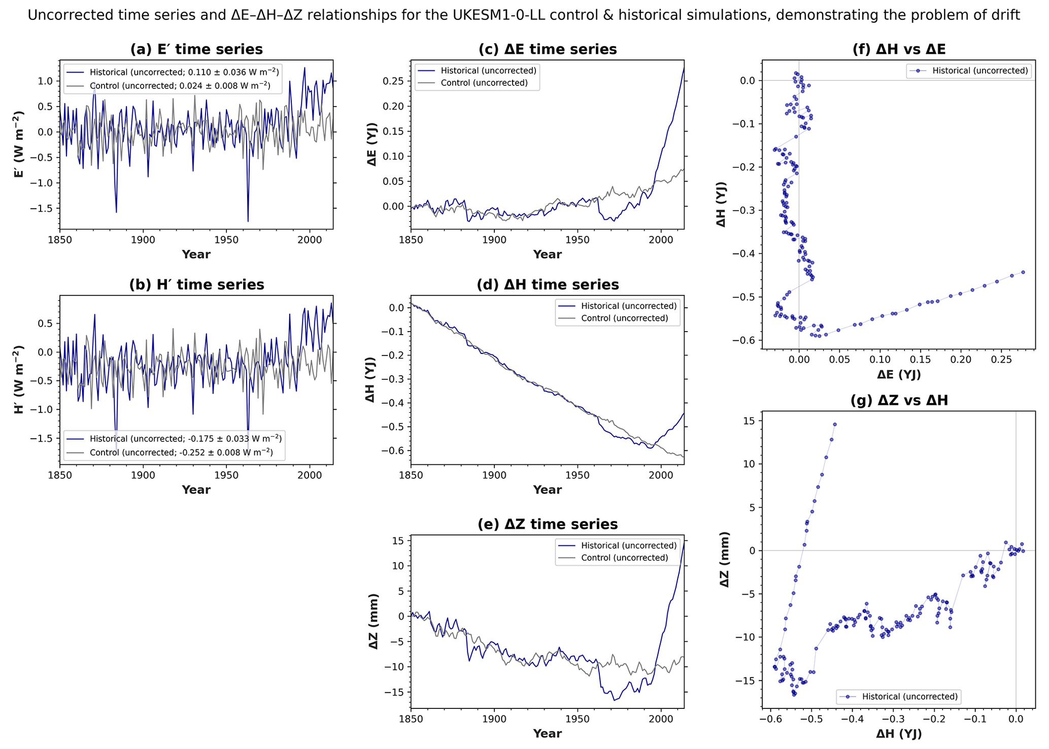
Figure 1 Uncorrected time series and bivariate relationships for the UK Earth System Model (UKESM1). These uncorrected time series have not yet been corrected for drift. Using data from the control and historical simulations, time series are shown for the following global variables: (a) top-of-atmosphere radiative flux (E^′), (b) sea surface heat flux (H^′), (c) excess system energy (ΔE), (d) excess ocean heat (ΔH), and (e) thermosteric sea level rise (ΔZ). Global total E^′ and H^′ are expressed in global mean units of watts per square metre (W m⁻²). In (a) and (b), the legend shows the mean of the entire time series and the standard error of the mean. In (a–e), only the segment of the control time series that corresponds to the historical period (1850–2014) is shown. (The full length of the entire control time series is 1100 years.) For the historical simulation, bivariate relationships are also shown: (f) ΔH versus ΔE and (g) ΔZ versus ΔH. Interpretation is offered in Sect. 4.1.

4 Results

4.1 Uncorrected time series

An example of drift is illustrated in Fig. 1. For UKESM1's control simulation, the top-of-atmosphere radiative flux (E^′) is close to zero (Fig. 1a), consistent with quasi-equilibrium radiative balance at the top of the atmosphere. The UKESM1 team have achieved their stated goal of keeping E^′ close to zero when tuning the model (Sellar et al., 2019). Therefore, the drift in excess system energy (ΔE) is small (Fig. 1c).

However, the sea surface heat flux (H^′) has a negative bias (Fig. 1b), showing that the ocean loses heat spuriously. When we integrate the flux cumulatively, the negative bias in H^′ integrates into a negative trend in excess ocean heat (ΔH; Fig. 1d). This illustrates the connection between bias and drift: a constant bias in a flux will drive a linear trend in the cumulatively integrated flux (Hobbs et al., 2016). In this example, the drift in ΔH also dominates the historical time series, obscuring the anthropogenic warming signal during the 20th century (Fig. 1d). Anthropogenic forcing only becomes strong enough to offset the negative bias in H^′ towards the end of the 20th century (Fig. 1b).

If energy is conserved within the modelled climate system, the ΔE–ΔH relationship should be approximately linear (Eq. A3). In contrast, for UKESM1's historical simulation, the drift in ΔH drives a strange ΔE–ΔH relationship (Fig. 1f): for most of the historical period, ΔE remains close to zero, but ΔH decreases. This reveals energy leakage. Furthermore, the inconsistency between ΔE and ΔH reveals that the energy leakage occurs somewhere between the top of the atmosphere and the sea surface (i.e. outside the ocean; Hobbs et al., 2016).

In this example, thermosteric sea level rise (ΔZ) also exhibits drift (Fig. 1e). The drift in ΔZ obscures the anthropogenic sea level rise signal during the 20th century. The drift will also contaminate future projections. Furthermore, the ΔH–ΔZ relationship (Fig. 1g) is inconsistent with Eq. (A4).

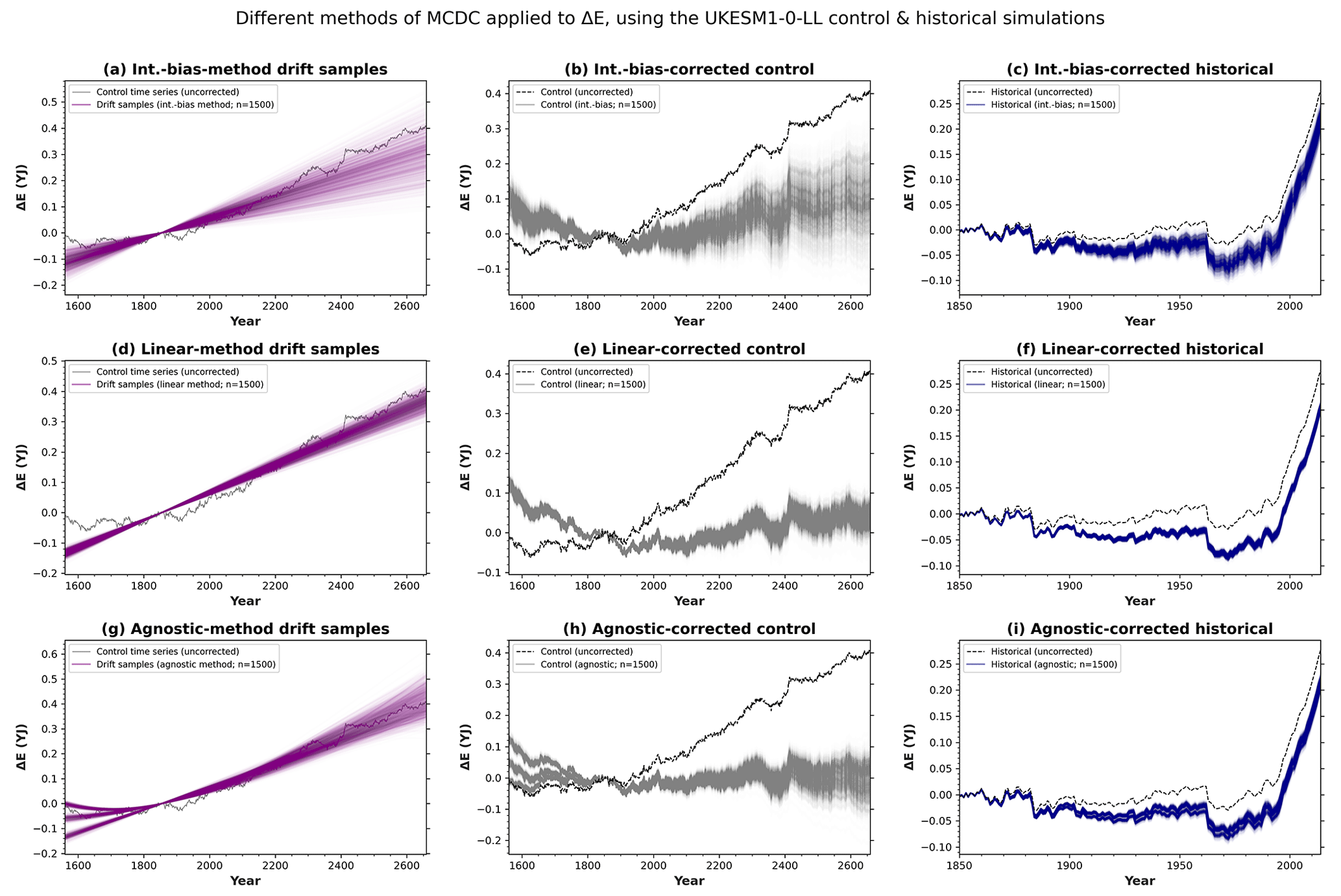
Figure 2 Different drift correction methods applied to excess system energy (ΔE) using the UKESM1 control and historical simulations. The first row (a–c) shows integrated-bias-method MCDC results: (a) drift samples derived using the integrated bias method, (b) integrated-bias-method drift-corrected control time series, and (c) integrated-bias-method drift-corrected historical time series, plotted alongside the uncorrected time series. The second row (d–f) shows corresponding linear-method MCDC results. The third row (g–i) shows corresponding agnostic-method MCDC results. These drift correction methods are described in Sect. 3.2.

4.2 Excess system energy (ΔE)

Figure 2 illustrates the application of MCDC to UKESM1's ΔE time series. For each MCDC method, we produce 1500 drift samples using the uncorrected control time series (Fig. 2a, d, and g). For UKESM1, these drift samples all indicate positive drift during the historical period. We subtract these drift samples from the uncorrected control time series to produce drift-corrected control time series (Fig. 2b, e, and h). In comparison to the uncorrected time series, the trends of these drift-corrected control time series are much closer to zero, as expected. We also subtract the drift samples from the uncorrected historical time series to produce drift-corrected historical time series (Fig. 2c, f, and i).

The spread among the drift samples and the drift-corrected time series indicates drift uncertainty. For UKESM1, the drift uncertainty is largest when integrated-bias-method MCDC is used (Fig. 2a–c). The linear-method drift uncertainty is much smaller (Fig. 2d–f). This demonstrates that integrated-bias-method MCDC and linear-method MCDC produce different estimates of drift uncertainty, even though these two methods have similar underlying assumptions – namely, a constant bias in E^′ drives a linear trend in ΔE. We ascribe the difference between the two methods to the size of the standard error: even if autocorrelation is accounted for, the standard error of the trend of ΔE is smaller than the standard error of the mean of E^′ because integrating cumulatively effectively averages over the substantial inter-annual variability in E^′. Therefore, integrated-bias-method MCDC provides a much weaker constraint on the drift correction. To minimise drift uncertainty, it is preferable to use linear-method MCDC.

However, the underlying drift may be non-linear. If so, a linear model of drift may be inappropriate. Therefore, linear-method MCDC will likely underestimate drift uncertainty. By partially accounting for the possibility of non-linearity, agnostic-method MCDC should provide a more accurate estimate of drift uncertainty. For UKESM1, agnostic-method drift uncertainty is larger than linear-method drift uncertainty yet smaller than integrated-bias drift uncertainty (Fig. 2; Table S2).

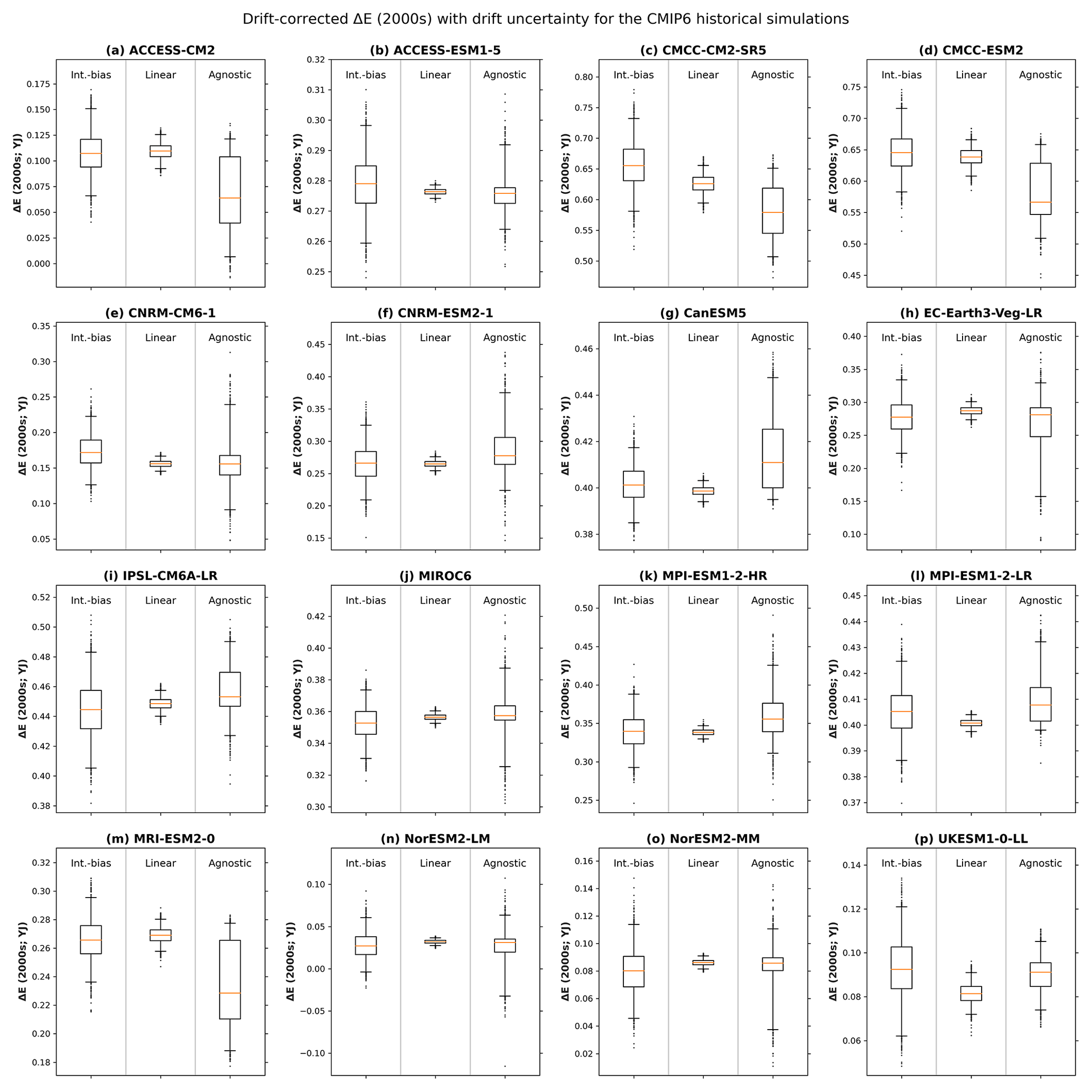
Figure 3 Drift-corrected excess system energy (ΔE) during the historical period and the corresponding drift uncertainty. We calculate ΔE as the decadal mean for the 2000s relative to the 1850s. Each panel shows results for one CMIP6 model (Table S1). Within each panel, each box plot shows results for one MCDC method. The central line shows the median, the box shows the interquartile range, the whiskers show the 2nd–98th inter-percentile range, and the dots show outliers beyond the range of the whiskers. Corresponding results for ΔH and ΔZ are shown in Figs. S1–S2.

Table 1 CMIP6 ensemble median and range (minimum–maximum) for different sources of uncertainty. For each drift correction method, drift uncertainty corresponds to the 2nd–98th inter-percentile range of the drift-corrected data. Model uncertainty corresponds to the inter-model range. Scenario uncertainty corresponds to the inter-scenario range. The statistics for η and ϵ are based on the 21st century projection simulations (2015–2100). The ensemble statistics shown here correspond to the summary statistics shown in Tables S2–S6. For further details, see Tables S2–S6.

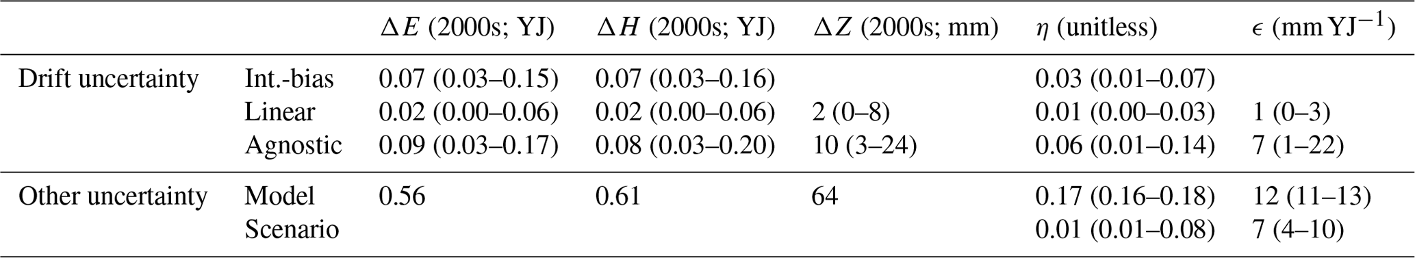
We extend our analysis to other global climate models within the CMIP6 ensemble by quantifying the drift uncertainty associated with ΔE during the historical period (2000s relative to 1850s; Fig. 3; Table S2). For all models, the linear-method drift uncertainty is substantially smaller than the integrated-bias-method drift uncertainty. The agnostic-method drift uncertainty is always larger than the linear-method drift uncertainty and is often larger than the integrated-bias-method drift uncertainty. When averaged across the ensemble, agnostic-method MCDC produces the largest estimate of drift uncertainty for ΔE, with a median of 0.09 YJ (Table 1). The ensemble maximum drift uncertainty is 0.17 YJ, approximately twice as large as the ensemble median (Table 1; Fig. 3h).

Differences between global climate models also drive differences in ΔE (Fig. 3). We refer to the inter-model range as model uncertainty (Tebaldi and Knutti, 2007; Knutti and Sedláček, 2013). For ΔE, the model uncertainty of 0.56 YJ is more than 3 times as large as the ensemble maximum drift uncertainty (Table 1).

4.3 Excess ocean heat (ΔH)

For each CMIP6 model, the drift uncertainty associated with ΔH (Fig. S1; Table S3) is similar to the drift uncertainty associated with ΔE. The ensemble statistics are very similar to those of ΔE (Table 1). Therefore, we can draw very similar conclusions for the ΔH results as we have for the ΔE results. This is not surprising because ΔH is closely related to ΔE: both consist of cumulatively integrated fluxes, and ΔH should track ΔE closely if the fraction of excess energy absorbed by the ocean (η) is close to 1.0 (Sect. 4.5; Appendix A).

4.4 Thermosteric sea level rise (ΔZ)

For ΔZ over the historical period (2000s relative to 1850s), the agnostic-method drift uncertainty is always larger than the linear-method drift uncertainty, as expected (Fig. S2; Table S4). (Integrated-bias-method MCDC is not applicable to ΔZ, which does not consist of a cumulatively integrated flux.) The agnostic-method drift uncertainty ranges from 3 to 24 mm, with an ensemble median of 10 mm (Table 1). This is smaller than the model uncertainty of 64 mm (Table 1). On the other hand, the drift uncertainty is of comparable magnitude to the impact of omitting volcanic forcing in control simulations: Gregory et al. (2013) found that neglecting pre-industrial volcanic forcing leads to an underestimate of 5–30 mm over the period 1850–2000. Furthermore, for models with relatively large drift uncertainty, the drift uncertainty may influence the extent to which the historical time series agrees with estimates of ΔZ derived from observations, such as the reconstructions of Zanna et al. (2019) and Frederikse et al. (2020). For two CMIP6 models, the agnostic-method drift uncertainty is large enough to obscure the positive ΔZ signal during the historical period: the 2nd–98th percentile range includes negative values of ΔZ (Fig. S2a and n).

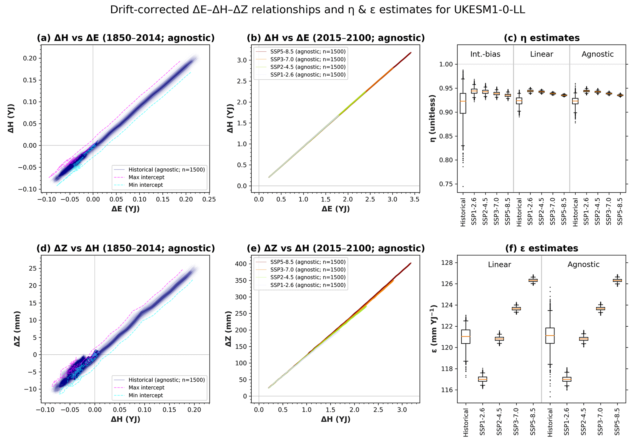
Figure 4 Drift-corrected bivariate relationships and regression coefficients (η and ϵ) for the UKESM1 simulations. (a–b) Agnostic-method drift-corrected excess ocean heat (ΔH) versus excess system energy (ΔE) for (a) the historical simulation and (b) the projection simulations. (c) Estimates of the fraction of excess energy absorbed by the ocean (η) and the corresponding drift uncertainty. The coefficient η is calculated as the linear regression coefficient of drift-corrected ΔH versus ΔE. For each combination of MCDC method and projection scenario, the central line shows the median, the box shows the interquartile range, the whiskers show the 2nd–98th inter-percentile range, and the dots show outliers beyond the range of the whiskers. (d–e) Agnostic-method thermosteric sea level rise (ΔZ) versus ΔH for (d) the historical simulation and (e) the projection simulations. (f) Estimates of the expansion efficiency of heat (ϵ) and the corresponding drift uncertainty. The coefficient ϵ is calculated as the linear regression coefficient of drift-corrected ΔZ versus ΔH. Corresponding estimates of η and ϵ for other members of the CMIP6 ensemble are shown in Figs. 5 and S3.

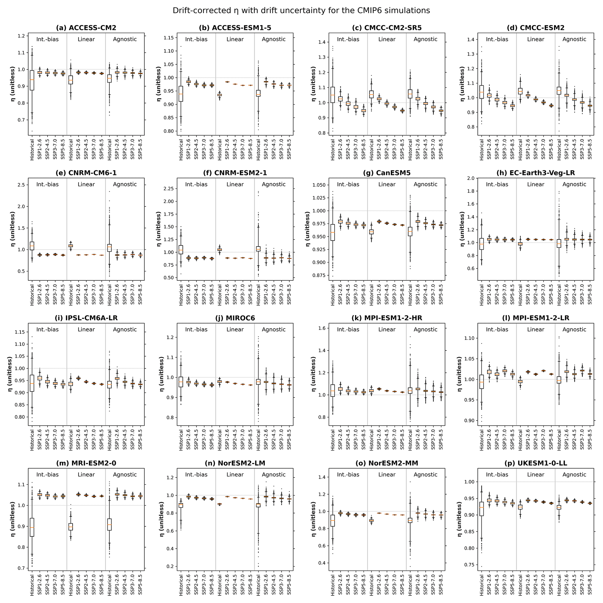
Figure 5 Drift-corrected estimates of the fraction of excess system energy absorbed by the ocean (η) and the corresponding drift uncertainty. Each panel shows results for one CMIP6 model. Within each panel, each box plot shows results for one combination of MCDC method and projection scenario. The central line shows the median, the box shows the interquartile range, the whiskers show the 2nd–98th inter-percentile range, and the dots show outliers beyond the range of the whiskers. The horizontal line at η=1.0 shows the theoretical maximum value of η.

4.5 Fraction of excess energy absorbed by the ocean (η)

If energy is conserved and if the fraction of excess energy absorbed by the ocean (η) is constant, then excess ocean heat (ΔH) should be a linear function of excess system energy (ΔE): ΔH=ηΔE (Eq. A3). However, as noted in Sect. 4.1 above, the uncorrected ΔE–ΔH relationship for UKESM1's historical time series is non-linear and reveals energy leakage (Fig. 1f). Can drift correction address this problem? After we apply agnostic-method MCDC, the trend-corrected ΔE–ΔH relationships are linear (Fig. 4a–b). Estimates of the coefficient η are positive and less than 1.0 (Fig. 4c). Therefore, for UKESM1, the drift-corrected ΔE–ΔH relationships are generally consistent with Eq. (A3).

When applying MCDC, we produce 1500 drift-corrected time series for each variable, scenario, model, and MCDC method. Therefore, we also calculate 1500 estimates of η, so we can quantify drift uncertainty. For all three MCDC methods, the drift uncertainty in η is relatively large during the historical period (Figs. 4c and 5): the relatively weak global warming signal in the ΔE and ΔH historical time series leaves them susceptible to drift uncertainty, which in turn influences the η estimates. The drift uncertainty in η is much smaller during the 21st century projection period (Figs. 4c and 5): global warming drives clear trends in the ΔE and ΔH projection time series, constraining the η estimates. We average across the projection simulations to summarise the drift uncertainty in η (Table S5; Table 1). For UKESM1, the agnostic-method drift uncertainty is approximately 0.01 (Table S5). Across the CMIP6 ensemble, the agnostic-method drift uncertainty ranges from 0.01 to 0.14, with a median of 0.06 (Table 1).

The η estimates differ slightly between the different projection simulations (Figs. 4c and 5). The differences arise from the response of the climate system to different forcing scenarios. We refer to the inter-scenario range as the scenario uncertainty. For the UKESM1 projection simulations, the scenario uncertainty is approximately 0.01, similar to the drift uncertainty (Table S5). For most models in the CMIP6 ensemble, the scenario uncertainty is similarly small (Fig. 5; Table S5), with an ensemble median of 0.01 (Table 1): in general, η does not depend strongly on the scenario. However, for two models, the scenario uncertainty is 0.08 and 0.07, respectively (Table S5; Fig. 5c–d): for these models, η is sensitive to the choice of scenario.

Estimates of η vary between different models within the ensemble (Fig. 5). The model uncertainty of 0.17 is the largest source of uncertainty (Table 1). For most of the CMIP6 models, the η estimates lie in the range 0.9–1.0, consistent with our understanding of the climate system (Appendix A; von Schuckmann et al., 2020; Forster et al., 2021): even if the ocean were to absorb all excess energy entering the climate system, this would lead to a theoretical maximum of 1.0. However, some of the η estimates are larger than 1.0. For four models (25 % of the ensemble), the median η estimates are consistently greater than 1.0 for all projection scenarios (Fig. 5h, k, l, and m): even after drift correction, the energy balance of these models remains problematic.

4.6 Expansion efficiency of heat (ϵ)

As the ocean warms, it expands, leading to thermosteric sea level rise. We expect the relationship between ΔH and ΔZ to be approximately linear: ΔZ=ϵΔH (Eq. A4). As noted in Sect. 4.1 above, the uncorrected data from UKESM1's historical simulation are inconsistent with Eq. (A4) (Fig. 1g). However, after we apply agnostic-method MCDC, the drift-corrected ΔH–ΔZ relationships are approximately linear (Fig. 4d and e). Drift correction successfully establishes meaningful ΔH–ΔZ relationships that can be interpreted using Eq. (A4).

However, in disagreement with Eq. (A4), the drift-corrected ΔH–ΔZ relationships during the historical period exhibit hysteresis-like behaviour (Fig. 4d). ΔH and ΔZ are referenced to the 1850s decadal mean, so the ΔH–ΔZ relationships begin near the origin. ΔH and ΔZ then become negative for much of the historical period, driving the relationships towards the lower left of Fig. 4d. ΔH and ΔZ become positive later in the historical period, driving the relationships towards the upper right. However, ΔH and ΔZ do not necessarily both become positive at the same time, so the relationships do not necessarily pass through the origin, as demonstrated by the “max intercept” and “min intercept” lines. It is possible that the ΔE–ΔH–ΔZ relationships may depend on the sign of the forcing (see Bouttes et al., 2013). However, the hysteresis-like behaviour in Fig. 4d – and also in Fig. 4a – does not reveal systemic hysteresis: for different MCDC samples, the intercept can be either negative or positive. Regardless of the explanations for this hysteresis-like behaviour, we use ordinary least squares with an intercept – not regression through the origin – to estimate the linear regression coefficient (Appendix B).

The linear regression coefficient is ϵ, the expansion efficiency of heat. As was the case for η, the drift uncertainty in ϵ is much larger during the historical period than the 21st century (Figs. 4f and S3) due to the comparatively weak forcing signal during the historical period. When drift uncertainty is considered, the historical period provides only a weak constraint on the value of ϵ.

For the UKESM1 projection simulations, the estimates of ϵ depend on the scenario, ranging from approximately 117 mm YJ⁻¹ (SSP1-2.6) to 126 mm YJ⁻¹ (SSP5-8.5; Fig. 4f). This scenario uncertainty of 9 mm YJ⁻¹ is much larger than the agnostic-method drift uncertainty of 1 mm YJ⁻¹ (Table S6), leading to distinct non-overlapping box plots for the projection scenarios (Fig. 4f). For all models in the CMIP6 ensemble, the ϵ estimates are smallest for SSP1-2.6 and largest for SSP5-8.5 (Fig. S3). This suggests that the thermal expansion of the ocean is sensitive to the forcing scenario and is not merely a linear function of ΔH (see also Wu et al., 2021). However, the strength of the dependence on scenario varies: across the ensemble, the scenario uncertainty varies from 4 to 10 mm YJ⁻¹, with a median of 7 mm YJ⁻¹ (Table 1).

The agnostic-method drift uncertainty varies over a wider range, from 1 to 22 mm YJ⁻¹, with a median of 7 mm YJ⁻¹ (Table 1). The linear-method drift uncertainty is much smaller, suggesting that linear-method MCDC underestimates the drift uncertainty. The model uncertainty is 12 mm YJ⁻¹. When analysing ϵ across the CMIP6 ensemble, drift uncertainty, scenario uncertainty, and model uncertainty all constitute substantial sources of uncertainty.

5 Discussion

5.1 Energy balance

Following Hobbs et al. (2016) and Irving et al. (2021), we have considered the energy budgets of global climate models. Inconsistent relationships between excess system energy (ΔE) and excess ocean heat (ΔH; Fig. 1f) are symptomatic of energy leakage outside the ocean domain (Hobbs et al., 2016). In agreement with Hobbs et al. (2016) and Irving et al. (2021), we have shown that drift correction can partially address this problem of energy leakage. Drift-corrected ΔE–ΔH relationships are approximately linear (Fig. 4a and b). For all 16 models analysed here, the coefficient η – the fraction of excess energy absorbed by the ocean – is positive (Fig. 5). For most of these models, η is also less than 1.0, consistent with energy conservation. However, even after drift correction, the energy balance of several models remains suspect: energy leakage is revealed by η estimates greater than 1.0. For four models, the median η estimates are greater than 1.0 for all projection scenarios (Fig. 5).

When evaluating the performance of global climate models, the coefficient η is a useful diagnostic. This diagnostic could be used alongside other diagnostics relating to energy balance, such as the diagnostics considered by Mayer et al. (2017) and Wild (2020).

5.2 Drift uncertainty

Sanderson (2020) previously explored the contribution of drift to uncertainty in global climate sensitivity indices. To do this, Sanderson added drift (via spurious forcing) and inter-annual variability (via noise) to a simple two-timescale response model. In contrast, we have quantified drift uncertainty directly from global climate model data using Monte Carlo drift correction (MCDC).

We have compared alternative methods of correcting drift in cumulatively integrated fluxes (such as ΔE and ΔH). When applying linear-method MCDC, the flux is first integrated cumulatively, and then the spurious trend is quantified and subtracted. When applying integrated-bias-method MCDC, the bias in the flux is first quantified and subtracted, and then the bias-corrected flux is integrated cumulatively. Conceptually, these two alternative approaches are similar: a constant bias in flux (e.g. E^′) will drive a spurious trend in cumulatively integrated flux (e.g. ΔE) (Hobbs et al., 2016). In practice, however, we find that these two alternative methods produce differing results: the linear-method drift uncertainty is smaller than the integrated-bias-method drift uncertainty because integrating cumulatively effectively averages over the substantial inter-annual variability, resulting in a smaller standard error. In other words, compared with integrated-bias-method MCDC, linear-method MCDC provides a much stronger constraint on the appropriate drift correction to apply. When correcting drift in an integrated variable, it is generally preferable to integrate the variable first and then apply the drift correction afterward. Nevertheless, we recognise that there may be cases for which it makes sense to correct the bias before integrating: for example, when performing an analysis that involves both E^′ and ΔE, we may prefer to use the integrated bias method for consistency. Researchers should clarify whether they correct drift before or after integration. Although we primarily refer to cumulative integration across time here, such clarity should also extend to other calculations: for example, Irving et al. (2019) clarify that they calculate spatial integrals before correcting drift.

When estimating drift uncertainty, our preferred method is agnostic-method MCDC. If the drift is non-linear, then linear-method MCDC will likely underestimate the drift uncertainty. Therefore, agnostic-method MCDC – which assigns equal prior probabilities to linear, quadratic, and cubic models of drift – should provide a more accurate estimate of drift uncertainty. For the variables analysed in this paper, we have found that agnostic-method drift uncertainty is larger than linear-method drift uncertainty, as expected. We emphasise that agnostic-method corresponds to an assumption that linear, quadratic, and cubic models of drift are all equally plausible. This assumption corresponds to the common practice of selecting a statistical model of drift a priori before fitting the model to data (Sect. 3.1).

A possible further step would be to fit and compare alternative statistical models of drift a posteriori using measures such as the Bayesian information criterion. We could then select the best statistical model(s) for a specific time series. When applying this “best-fit” approach, we could also consider additional statistical models of drift, including signal processing filters (e.g. Palmer et al., 2011). This best-fit approach would be a sensible way to correct drift. Application of the best-fit approach should lead to a reduction in drift uncertainty.

It may be important to quantify drift uncertainty when analysing time series with a relatively weak trend. In particular, historical time series may be susceptible to drift uncertainty. For the historical period, the agnostic-method drift uncertainty in ΔZ can be as large as 24 mm, which is of comparable magnitude to the impact of omitting volcanic forcing in control simulations (Gregory et al., 2013). Therefore, drift uncertainty deserves similar attention to that given to volcanic forcing.

We hypothesise that drift uncertainty may influence the extent to which a historical simulation agrees with an observation-based estimate. Drift uncertainty should be considered when comparing historical simulations with observation-based estimates of thermosteric sea level change (such as the reconstruction of Frederikse et al., 2020). Drift uncertainty should also be considered when using ocean-related variables – such as ocean heat content (Lyu et al., 2021) – as an emergent constraint for global climate models.

We further hypothesise that drift uncertainty may be large for drift-susceptible time series that exhibit large internal variability, such as regional dynamic sea level (Richter et al., 2020; Hamlington et al., 2021). Large variability will lead to a large standard error when fitting the statistical model of drift. Therefore, drift uncertainty should be considered when analysing time series with large internal variability, provided that the time series is known to be susceptible to drift.

On the other hand, drift is often weak for time series unrelated to the deep ocean (Sen Gupta et al., 2013). Therefore, many analyses – such as multi-model mean hemispheric partitioning of upper-ocean heat – may be insensitive to drift (Durack et al., 2014). In such cases, drift correction may be unnecessary and drift uncertainty may be ignored.

In this study, we have focused on global variables. When correcting drift in multivariate regional contexts – such as might be done in preparation for dynamical downscaling – drift correction approaches may be informed by additional considerations to ensure consistency (Paeth et al., 2019). Furthermore, we have focused on correcting drift in long-term climate simulations, which are dominated by external forcing. In contrast, shorter-term decadal simulations are further complicated by observation-based initialisation; hence, decadal simulations require different drift correction methods (Choudhury et al., 2017; Hossain et al., 2021). The quantification of drift uncertainty in such contexts remains an open question.

6 Conclusions

We have developed a probabilistic technique: Monte Carlo drift correction (MCDC). MCDC has enabled us to quantify the drift uncertainty of global climate models.

We have also considered a problem related to drift: energy leakage. Although energy leakage is partially addressed by drift correction, the energy balance of some CMIP6 models remains suspect. Following drift correction, a useful diagnostic for model evaluation is provided by the coefficient η (the fraction of excess energy absorbed by the ocean): is η≤1?

We draw four conclusions about drift correction.

1. When correcting drift in cumulatively integrated fluxes (e.g. ΔE, the excess system energy), it is generally preferable to integrate the fluxes before correcting the drift rather than correcting the bias before integrating the fluxes.

2. Linear-method MCDC may underestimate drift uncertainty due to non-linearity in the underlying drift. If we assume that linear, quadratic, and cubic statistical models of drift are equally plausible, then agnostic-method MCDC provides a more accurate estimate of drift uncertainty.

3. When analysing ΔZ (thermosteric sea level rise) during the historical period, drift uncertainty is relatively large. For the period 1850s–2000s, the agnostic-method drift uncertainty ranges from 3 to 24 mm. This is comparable to the impact of omitting volcanic forcing in control simulations (Gregory et al., 2013).

4. When using 21st century projection scenarios to estimate ϵ (the expansion efficiency of heat), agnostic-method drift uncertainty of 1 to 22 mm YJ⁻¹ constitutes an important source of uncertainty alongside scenario uncertainty and model uncertainty.

We propose two hypotheses – each with an accompanying question – to be tested in future work. First, drift uncertainty will influence the extent to which a historical simulation agrees with observation-based estimates. In light of this, can ocean-related variables still be used as emergent constraints for the evaluation of global climate models? Second, drift uncertainty will be large for regional variables with large internal variability, such as dynamic sea level change. What are the implications for climate projections?

Finally, we offer one recommendation: when evaluating and analysing data that are prone to drift, researchers should consider the potential influence of drift uncertainty.

Appendix A: Equations connecting energy fluxes, excess energy, and thermosteric sea level rise

If the Earth's climate system were in equilibrium, the incoming and outgoing energy fluxes would balance (Meyssignac et al., 2019; Wild, 2020). In reality, the energy fluxes vary due to internal variability, leading to a quasi-equilibrium state that approximates equilibrium when averaged over long timescales. When the Earth's climate system experiences an external forcing – such as that caused by rising concentrations of greenhouse gases – the energy fluxes no longer balance.

A net downward top-of-atmosphere radiative flux (E^′) heats the Earth's climate system (Melet and Meyssignac, 2015; von Schuckmann et al., 2020), increasing the excess system energy (ΔE). Most of this excess system energy is transferred to the ocean via a net downward sea surface heat flux (H^′), increasing the ocean heat content (Meyssignac et al., 2019) – here, we refer to the change in ocean heat content as the excess ocean heat (ΔH). As the ocean warms, the water expands due to thermal expansion, causing thermosteric sea level rise (ΔZ; Gregory et al., 2019). To a first approximation, the relationships between these variables can be described using relatively simple equations. Following Melet and Meyssignac (2015), we describe the equations below.

We begin by noting that the total excess energy that enters the Earth's climate system can be calculated by integrating the global total top-of-atmosphere radiative flux (E^′) cumulatively over time:

$$\begin{array}{}\text{(A1)}& \text{Excess system energy}\equiv \mathrm{\Delta }E\equiv \underset{t_{\mathrm{0}}}{\overset{t}{\int }}{E}^{\prime }\left(\mathit{\tau }\right)\mathrm{d}\mathit{\tau },\end{array}$$

where t₀ is the reference time. Expressed in global mean units, E^′ is estimated to be 0.47 ± 0.1 W m⁻² for the period 1971–2018 and is increasing (von Schuckmann et al., 2020).

On annual to decadal timescales and longer, most excess system energy is absorbed by the ocean (Palmer et al., 2011; Palmer and McNeall, 2014; Durack et al., 2018; Meyssignac et al., 2019). The change in ocean heat content can be calculated by integrating the global total sea surface heat flux (H^′) cumulatively over time:

$$\begin{array}{}\text{(A2)}& \text{Excess ocean heat}\equiv \mathrm{\Delta }H\equiv \underset{t_{\mathrm{0}}}{\overset{t}{\int }}{H}^{\prime }\left(\mathit{\tau }\right)\mathrm{d}\mathit{\tau }.\end{array}$$

A constant geothermal heat flux of approximately 0.1 W m⁻² (Davies and Davies, 2010) also contributes to ocean heat content. We ignore this geothermal heat flux – which is much smaller than E^′ – to focus on the relationship between E^′ and H^′. The drift-corrected ΔH time series should be insensitive to the inclusion or exclusion of the geothermal heat flux: a constant geothermal heat flux would essentially modify the bias in H^′ and the linear drift in ΔH, both of which are removed by drift correction.

If we assume that the fraction of excess energy absorbed by the ocean (η) is constant, then the excess ocean heat can be written as a linear function of the excess system energy:

$$\begin{array}{}\text{(A3)}& \mathrm{\Delta }H=\mathit{\eta }\mathrm{\Delta }E.\end{array}$$

For the period 1971–2018, η is estimated to be approximately 0.89–0.91 (von Schuckmann et al., 2020; Forster et al., 2021).

As the ocean warms, the water expands, causing thermosteric sea level rise (Gregory et al., 2019). The thermal expansion of water varies between locations and depths, increasing with temperature, salinity, and pressure (Russell et al., 2000; Piecuch and Ponte, 2014). Remarkably, the thermal expansion coefficient is an order of magnitude larger in the warm low-latitude ocean than it is in the cold high-latitude ocean (Griffies and Greatbatch, 2012). Nevertheless, in practice, we can use a globally representative coefficient: ϵ, the “expansion efficiency of heat” (Russell et al., 2000). Global mean thermosteric sea level rise (ΔZ) can then be written as a linear function of excess ocean heat (Kuhlbrodt and Gregory, 2012; Melet and Meyssignac, 2015):

$$\begin{array}{}\text{(A4)}& \mathrm{\Delta }Z=\mathit{ϵ}\mathrm{\Delta }H.\end{array}$$

For the period 1995–2014, ϵ is estimated to be 121 ± 1 mm YJ⁻¹ (Fox-Kemper et al., 2021).

Appendix B: Estimating η and ϵ using ordinary least squares

Informed by Eqs. (A3) and (A4), we estimate η and ϵ using linear regression. Should we use ordinary least squares with an intercept or regression through the origin (Eisenhauer, 2003)? Regression through the origin is controversial yet sometimes justifiable (Eisenhauer, 2003). In this particular case, Eqs. (A3) and (A4) provide strong theoretical support for the application of regression through the origin. We would expect Eqs. (A3) and (A4) to hold across the full range of the climate model time series, including the origin (because ΔE, ΔH, and ΔZ are all referenced to the 1850s decadal mean).

However, the drift-corrected ΔE–ΔH and ΔH–ΔZ relationships often exhibit hysteresis-like behaviour during the historical period (Figs. 4a and d, especially the “max intercept” and “min intercept” lines): when the time series transition from negative values to positive values, the ΔE–ΔH and ΔH–ΔZ relationships do not necessarily pass through the origin. Such hysteresis-like behaviour during the historical period influences the starting point of the projection time series. This undermines the appropriateness of regression through the origin. Furthermore, we are interested primarily in linear relationships within the range of data for any given scenario. For example, when estimating η and ϵ for a projection scenario, we are interested in the relationship over the period 2015–2100. In light of these considerations, we use ordinary least squares with an intercept.