the Creative Commons Attribution 4.0 License.
the Creative Commons Attribution 4.0 License.
 | 14 Nov 2023
Machine learning for numerical weather and climate modelling: a review
Catherine O. de Burgh-Day
Tennessee Leeuwenburg
Machine learning (ML) is increasing in popularity in the field of weather and climate modelling. Applications range from improved solvers and preconditioners, to parameterization scheme emulation and replacement, and more recently even to full ML-based weather and climate prediction models. While ML has been used in this space for more than 25 years, it is only in the last 10 or so years that progress has accelerated to the point that ML applications are becoming competitive with numerical knowledge-based alternatives. In this review, we provide a roughly chronological summary of the application of ML to aspects of weather and climate modelling from early publications through to the latest progress at the time of writing. We also provide an overview of key ML terms, methodologies, and ethical considerations. Finally, we discuss some potentially beneficial future research directions. Our aim is to provide a primer for researchers and model developers to rapidly familiarize and update themselves with the world of ML in the context of weather and climate models.


Current state-of-the-art weather and climate models use numerical methods to solve equations representing the dynamics of the atmosphere and ocean on meshed grids. The grid-scale effects of processes that are too small to be resolved are either represented by parametrization schemes or prescribed. These numerical weather and climate forecasts are computationally costly and are not easy to implement on specialized compute resources such as graphics processing units†1 (GPUs; although there are efforts underway to do so, for example in LFRic; Adams et al., 2019). One of the main approaches to improving forecast accuracy is to increase model resolution (reduced time step between model increments and/or decreased grid spacing), but due to the high computational cost of this approach, improvements in model skill are hampered by the finite supercomputer capacity available. An additional pathway to improve skill is to improve the understanding and representation of subgrid-scale processes; however this is again a potentially computationally costly exercise.
In the remainder of this introduction, we overview the state of machine learning in weather and climate research without always providing references; we instead provide relevant references in the detailed sections that follow.
Machine learning is an increasingly powerful and popular tool. It has proven to be computationally efficient, as well as being an accurate way to model subgrid-scale processes. The term “machine learning” (ML) was first coined by Arthur Samuel in the 1950s to refer to a “field of study that gives computers the ability to learn without being explicitly programmed” (http://infolab.stanford.edu/pub/voy/museum/samuel.html, last access: 7 February 2023). Learning by example is the defining characteristic of ML.
The growing potential for ML in weather and climate modelling is being increasingly recognized by meteorological agencies and researchers around the world. The former is evidenced by the development of strategies and frameworks to better support the development of ML research, such as the Data Science Framework recently published by the Met Office in the UK (https://www.metoffice.gov.uk/research/foundation/informatics-lab/met-office-data-science-framework, last access: 7 February 2023). The latter is made clear by the explosion in publications from academia, government agencies, and private industry in this space, as demonstrated by the rest of this review. Figure 1 shows the number of publications cited in this review using different categories of ML algorithms by year, and it clearly illustrates the increase in the uptake of ML methods by the research community.
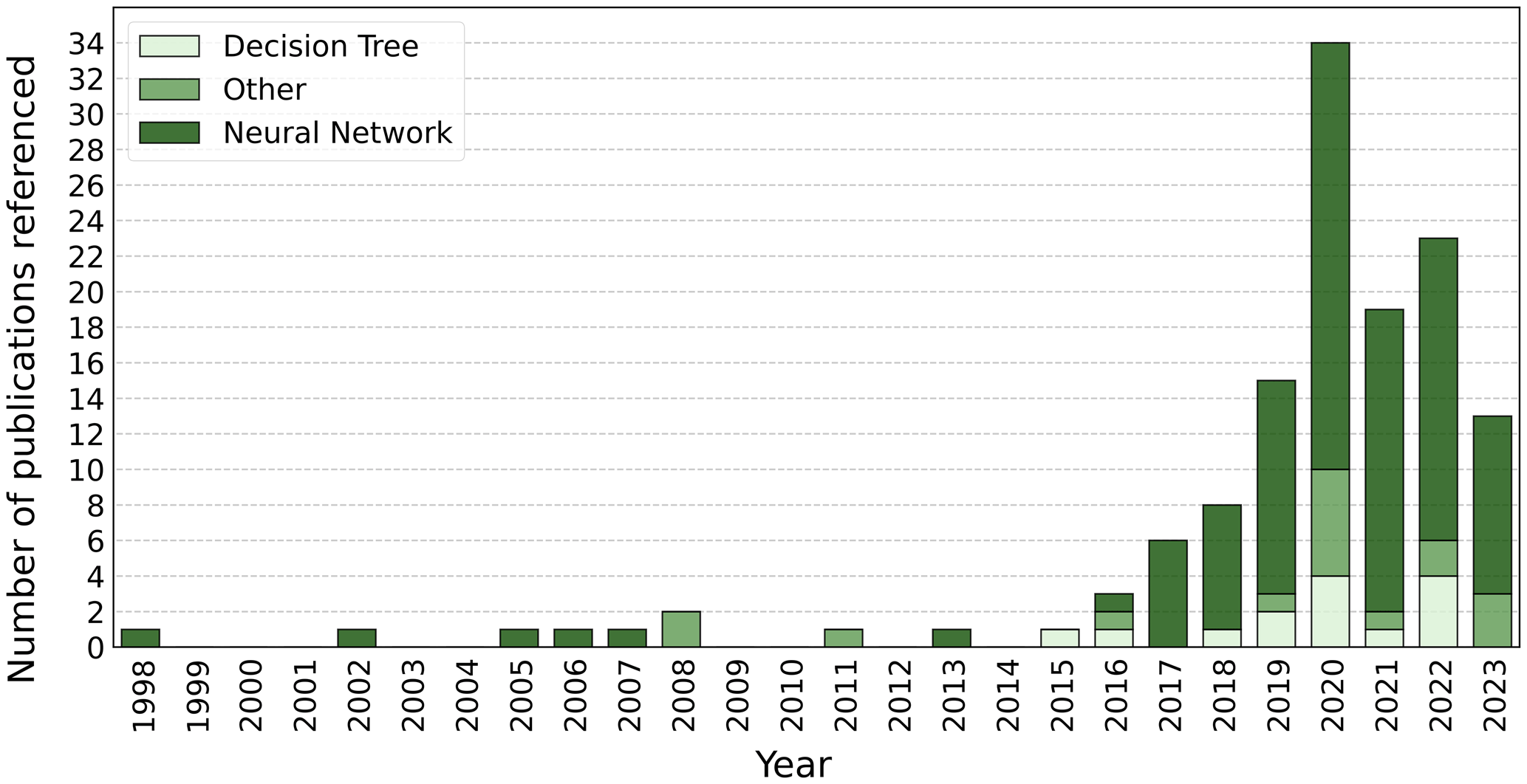
Figure 1A stacked bar graph of the number of publications cited in this review using different categories of ML algorithms by per year. For a description of neural networks and decision trees see Sect. 2.1 and 2.2 respectively. The “other” category is a collection of ML model types other than decision trees and neural networks, each of which only had one or two examples of use in this review. This included custom supervised and self-supervised algorithms, support vector machines and relevance vector machine models, regression models, unsupervised learning models, reservoir computing models, and non-NN Gaussian models. This figure includes all references from this review except for seminal ML papers that are on new ML methods (e.g. foundational ML papers from outside the domain of weather and climate modelling), review papers, any paper cited that concerns a topic which is out of scope (e.g. nowcasting), and any other paper which does not present a new method directly applicable to weather and climate modelling. The full table of citations is provided in Appendix A.
This is not necessarily an unbiased sample of the use of different architectures in the literature since the selection of papers cited in this review focuses on telling the story of the growth of the use of ML in weather and climate modelling over time rather than being a comprehensive list of all uses of ML in the literature.
There are established techniques and aspects of the weather and climate modelling lifecycle that would already be considered ML by many. For example, linear regression†, principal component analysis, correlations, and the calculation of teleconnections can all be considered types of ML. Data assimilation techniques could also be considered a form of ML. There are, however, other classes of ML (e.g. neural networks† and decision trees†) which are much less widely used within the weather and climate modelling space but have great potential to be of benefit. There is growing interest in, and increasingly effective application of, these ML techniques to take the place of more traditional approaches to modelling. The potential for ML in weather and climate modelling extends all the way from replacement of individual sub-components of the model (to improve accuracy and reduce computational cost) to full replacement of the entire numerical model.
While ML models are typically computationally costly during training, they can provide very fast predictions at inference† time, especially on GPU hardware. They often also avoid the need to have a full understanding of the processes being represented and can learn and infer complex relationships without any need for them to be explicitly encoded. These properties make ML an attractive alternative to traditional parametrization, numerical solver, and modelling methods.
Neural networks (NNs, explained further in Sect. 2.1) in particular are an increasingly favoured alternative approach for representing subgrid-scale processes or replacing numerical models entirely. They consist of several interconnected layers† of non-linear nodes†, with the number of intermediate layers depending on the complexity of the system being represented. These nodes allow for the encoding of an arbitrary number of interrelationships between arbitrary parameters to represent the system, removing the need to explicitly encode these interrelationships into a parameterization or numerical model.
One challenge that must be overcome before there will be more widespread acceptance of ML as an alternative to traditional modelling methods is that ML is seen as lacking interpretability. Most ML models do not explicitly represent the physical processes they are simulating, although physics-constrained ML is a new and growing field which goes some way to addressing this (see Sect. 6). Furthermore, the techniques available to gain insight into the relative importance and predictive mechanism of each predictor (i.e. the model outputs) are limited. In contrast, traditional models are usually driven by some understanding and/or representation of the physical mechanisms and processes which are occurring. This makes it possible to more easily gain insight into what physical drivers could explain a given output. The “black box” nature of many current ML approaches to parametrization makes them an unpopular choice for many researchers (and can be off-putting for decision makers) since, for example, explaining what went wrong in a model after a bad forecast can be more challenging if there are processes in the model which are not, and cannot, be understood through the lens of physics. However, increasing attention is being paid to the interpretability of ML models (e.g. McGovern et al., 2019; Toms et al., 2020; Samek et al., 2021), and there are existing methods to provide greater insight into the way physical information is propagated through them (e.g. attention maps, which identify the regions in spatial input data that have the greatest impact on the output field, and ablation studies, which involve comparing reduced data sources and/or models to the original models that have full access to available data to gain insight into the models).
As with their traditional counterparts, ML-based parametrizations and emulators are typically initially developed in single-column models, aquaplanet configurations, or otherwise simplified models. There are many examples of ML-based schemes which have been shown to perform well against benchmark alternatives in this setting, only to fail to do so in a realistic model setting. A common theme is that these ML schemes rapidly excite instabilities in the model as errors in the ML parametrization push key parameters outside of the domain of the training data as the overall model is integrated forward in time, leading to rapidly escalating errors and to the model “blowing up”. Similarly, many ML-based full-model replacements perform well for short lead times, only to exhibit model drift and a rapid loss of skill for longer lead times due to rapidly growing errors and the model drifting outside its training envelope.
In recent years, however, progress has been made in developing ML parametrizations which are stable within realistic models (i.e. not toy models, aquaplanets, etc.), as well as ML-based full models which can run stably and skilfully to longer lead times. This is usually achieved through training the model on more comprehensive data, employing ML architectures which keep the model outputs within physically real limits or imposing physical constraints or conservation rules within the ML architecture or training loss functions†.
There are still challenges and possible limitations to an ML approach to weather and climate modelling. In most cases, a robust ML model or parameterization scheme should be able to
-
remain stable in a full (i.e. non-idealized) model run
-
generalize to cases outside its training envelope
-
conserve energy and achieve the required closures.
Additionally, for an ML approach to be worthwhile it must provide one or more of the following benefits:
-
for ML parametrization schemes,
- –
a speedup of the representation of a subgrid-scale process vs. when run with a traditional parametrization scheme, which can make the difference between the scheme being cost-effective to run or not – when it is not cost-effective the process usually needs to be represented with a static forcing or boundary condition file;
- –
a speedup of the model vs. when run with traditional parametrization schemes;
- –
improved representation of subgrid process(es) over traditional parameterization schemes, as measured by metrics appropriate to the situation;
- –
improved overall accuracy and/or skill of the model when run with traditional parametrization schemes;
- –
insight into physical processes not provided by current numerical models or theory;
- –
-
for full ML models,
- –
a speedup of the model vs. an appropriate numerical model control;
- –
improved overall accuracy and/or skill of the model vs. an appropriate numerical model control;
- –
skilful prediction to greater lead times than an appropriate numerical model control;
- –
insight into physical processes not provided by current numerical models or theory.
- –
Furthermore, in some cases of ML approaches to weather and climate modelling problems (particularly for full-model replacement) the work is led by data scientists and ML researchers with limited expertise in weather and climate model evaluation. This can lead to flawed, misleading, or incomplete evaluations. Hewamalage et al. (2022) have sought to rectify this problem by providing a guide to forecast evaluation for data scientists.
The scope of this review is deliberately limited to the application of ML within numerical weather and climate models or to their replacement. This is done to keep the length of this review manageable. ML has enormous utility for other aspects of the forecast value chain such as observation quality assurance, data assimilation, model output postprocessing, forecast product generation, downscaling, impact prediction, and decision support tools. A review of the application of, and progress in, ML in these areas would be of great value but is outside the scope of this review and is left to other work. Molina et al. (2023) have provided a very useful review of ML for climate variability and extremes which is highly complementary to this review. They draw similar lines of delineation in the earth system modelling (ESM) value chain to those mentioned above; describing them as “initializing the ESM, running the ESM, and postprocessing ESM output”. They examine each of these steps in turn, with a focus on the prediction of climate variability and extremes. Here we take a different approach, focusing on one part of the value chain (running the ESM) but looking in more detail at this one part. Additionally, here we consider climate modelling in the context of multiyear and free-running multidecadal simulations but exclude the topic of ML for climate change projections, climate scenarios, and multi-sector dynamics. This is again in the interests of ensuring the scope of the review is manageable rather than because these topics are not worthy of review. On the contrary, a review dedicated to the utility of machine learning in this area would be of enormous value to the community but cannot be adequately explored here. A brief introduction to key ML architectures and concepts, including suggested foundational reading, is also provided to aid readers who are unfamiliar with the subject.
The remainder of this review is structured as follows: in Sect. 2 an introduction to the two ML architectures most prevalent in the review is provided, followed by a suggested methodological approach to applying ML to a problem and finally a brief overview of some of the major ML architectures and algorithms. With this background in place, the application of ML in weather and climate modelling is explored in the following five sections. In Sect. 3, ML use in subgrid parametrization and emulation, along with tools and challenges specific to this domain, are covered. Zooming out from subgrid-scale to processes resolved on the model grid, in Sect. 4 the application of ML for the partial differential equations governing fluid flow is reviewed. Expanding the scope further again to consider the entire system, the use of ML for full-model replacement or emulation is reviewed in Sect. 5. In Sect. 6 the growing field of physics-constrained ML models is introduced, and in Sect. 7 a number of topics tangential to the main focus of this review are briefly mentioned. Setting the work covered in the previous sections in a broader context, a review of the history of, and progress in, ML outside of the fields of weather and climate science is presented in Sect. 8. In Sect. 9 some practical considerations for the integration of ML innovations into operational and climate models are discussed, followed by a short introduction to some of the ethical considerations associated with the use of ML in weather and climate modelling in Sect. 10. In Sect. 11, some future research directions are speculated on, and some suggestions are made for promising areas for progression. Finally, a summary is presented in Sect. 12, and a glossary of terms is provided after the final section to aid the reader in their understanding of key concepts and words (Appendix B).
While the scope of this paper is a review of ML work directly applicable to weather and climate modelling, an abridged introduction to some key fundamental ML concepts is provided here to aid the reader. Suggested starting points for interested readers, including guidance on the utility of different model architectures and algorithms, as well as the connections between different applications and approaches, are as follows:
-
Hsieh (2023) provides a thorough textbook on environmental data science including statistics and machine learning.
-
Chase et al. (2022a, b) provide an introduction to various machine learning algorithms with worked examples in a tutorial format and an excellent on-ramp to ML for weather and climate modelling.
-
Russell and Norvig (2021) provide a comprehensive book regarding artificial intelligence in general.
-
Goodfellow et al. (2016) provide a well-regarded book on deep learning theory and modern practise.
-
Hastie et al. (2009) provide a book on statistics and machine learning theory.
This introductory section is a brief exposition of the concepts most central to this review. Definitions for this section can be found in the glossary.
The majority of ML methods which have found traction in weather and climate modelling were first developed in fields such as computer vision, natural language processing, and statistical modelling. Few, if any, of the methods mentioned in this paper could be considered unique to weather and climate modelling; however they have in many cases been modified to a greater or lesser extent to suit the characteristics of the problem. In this review, the term algorithm refers to the mathematical underpinnings of a machine learning approach. By this definition, decision trees (DTs), NNs, linear regression, and Fourier transforms are examples of algorithms. The two most relevant algorithms for this review are DTs and NNs. Many ML algorithms can be thought of as optimizing a non-linear regression, with deep learning utilizing an extremely high-dimensional model. There is no consensus on the definition of ML, with the term encompassing relatively large or small topical domains depending on who is asked. A good rule of thumb, however, is that any iterative computational process that seeks to minimize a loss function or optimize an objective function can be considered to be a form of ML. Some of the chief concerns in machine learning are generalizability of the models, how to train (optimize the variables of) the model, and how to ensure robustness. The inputs and outputs of machine learning models are often the same as physical models or model components. The term architecture in machine learning refers to a specific way of utilizing an algorithm to achieve a modelling objective reliably. For example, the U-Net† architecture is a specific way of laying out an NN which has proven effective in many applications. The extreme gradient boosting decision tree† architecture is a specific way of utilizing DTs which has proven reliable and effective for an extraordinary number of problems and situations and is an excellent choice as a first tool to experiment with machine learning.
A major current focus of ML research in the context of weather and climate modelling is new NN-based architectures and algorithms, as well as improved training regimes. Many other algorithms have been and continue to be employed in machine learning more broadly but are not pertinent to this review.
A key point for ML researchers to be aware of is the critical importance of approaching model training carefully. There are many pitfalls which can result in underperformance, unexpected bias, or misclassification. For instance, adversarial examples† can occur “naturally”, and systems which process data can be subject to adversarial attack† through the intentional supply of data designed to fool a trained network.
2.1 Introduction to neural networks
NNs can be regarded as universal function approximators (Hornik et al., 1989; see also Lu et al., 2019). Further, NN architectures can theoretically be themselves modelled as a very wide feed-forward† NN with a single hidden layer†. A Fourier transform is another example of a function approximator, although it is not universal since not all functions are periodic. NNs can therefore theoretically be candidates for the accurate modelling of physical processes, although in practise they cannot always reliably interpolate beyond their training envelope and as such may not generalize to new regimes. ML models are typically introduced in the literature as being either classification† or regression† models and either supervised† or unsupervised†.
The mathematical underpinning of an NN can be considered distinctly in terms of its evaluation† (i.e. output, or prediction) step and its training update step. The prediction step can be considered as the evaluation of a many dimensional arbitrarily complex function.
The simplest NN is a single-input, single node network with a simple activation† function. A commonly used activation function for a single neuron is the sigmoid function, which helpfully compresses the range between 0 and 1 while allowing a non-linear response. A classification model will employ a threshold to map the output into the target categories. A regression model seeks to optimize the output result against some target value for the function. Larger networks make more use of linear activations and may utilize heterogenous activation function choices at different layers.
Complex NNs are built up from many individual nodes, which may have heterogenous activation functions and a complex connectome†. The forward pass†, by which inputs are fed into the network and evaluated against activation functions to produce the final prediction, uses computationally efficient processes to quickly produce the result.
The training step for an NN is far more complex. The earliest NNs were designed by hand rather than through automation. The training step applies a back-propagation† algorithm to apply adjustment factors to the weights† and biases† of each node based on the accuracy of the overall prediction from the network.
Training very large networks was initially impractical. Both hardware and architecture advances have changed this, resulting in the significant increase in the application of NNs to practical problems. Most NN research explores how to utilize different architectures to train more effective networks. There is little research going into improving the prediction step as the effectiveness of a network is limited by its ability to learn rather than its ability to predict. Some research into computational efficiency is relevant to the predictive step. NNs can still be technically challenging to work with, and a lot of skill and knowledge are needed to approach new applications.
The major classes of NN architectures most likely to be encountered are
-
small, fully connected networks, which are less commonly featured in recent publications but are still effective for many tasks and are still being applied and may well be encountered in practice;
-
convolutional† architectures, first applied to image content recognition, which match the connectome of the network to the fine structure of images in hierarchical fashion to learn to recognize high-level objects in images;
-
recurrent token†-sequence architectures, first applied to natural language processing, generation, and translation – applicable to any time-series problem – but now also applied to image and video applications, as well as mixed-mode applications such as text-to-image or text-to-video;
-
transformer architectures†, based on the attention mechanism† to provide a non-recurrent architecture that can be trained using parallelized training strategies, which allows larger models to be trained (originally developed for sequence prediction and extended to images processed through vision transformer architectures).
2.2 Introduction to decision trees
DTs are a series of decision points, typically represented in binary fashion based on a simple threshold. A particular DT of a particular size maps the input conditions into a final “leaf” node† which represents the outcome of the decisions up to that point.
A random forest† (RF) is the composition of a large number of DTs assembled according to a prescribed generation scheme, which are used as an ensemble. A gradient-boosted decision tree (GBDT) is built up sequentially, where each subsequent decision tree attempts to model the errors in the stack of trees built up thus far. This approach outperforms RFs in most cases.
The DT family of ML architectures are very easy to train and are very efficient. They are well documented in the public domain and in published literature. DTs are statistical in nature and are not capable of effectively generalizing to situations which are not similar to those seen during training. This can be an advantage when unbounded outputs would be problematic; however it can lead to problems where an ability to produce out-of-training solutions is necessary. Additionally, current DT implementations require all nodes (of all trees in the case of RFs and GBDTs) to be held in memory at inference time, making them potentially memory heavy.
2.3 Methodologies for machine learning
It is challenging to provide simplified advice for how to approach problem-solving in ML. There are few strict theoretical reasons to choose any one of the variety of architectures which are available. The authors would also caution against assuming that results in the literature are the product of a detailed comparison of alternative architectures or assuming that a deep learning approach is going to be easy or straightforward. It will often be the case that multiple machine learning architectures may be similarly effective, and determining the optimal architecture is likely to involve extensive iteration. Any specific methodology is also likely to reflect the intuitions (or biases), knowledge, and background of the authors of that methodology.
Nonetheless, there is an appetite from many scientists for reasonable ways to “get started” and to provide some assistance for practical decision-making, particularly if approaching the utilization of machine learning for the first time or in a new way. Figure 2 provides a set of suggested steps and decision points to help readers approach a new challenge with ML.
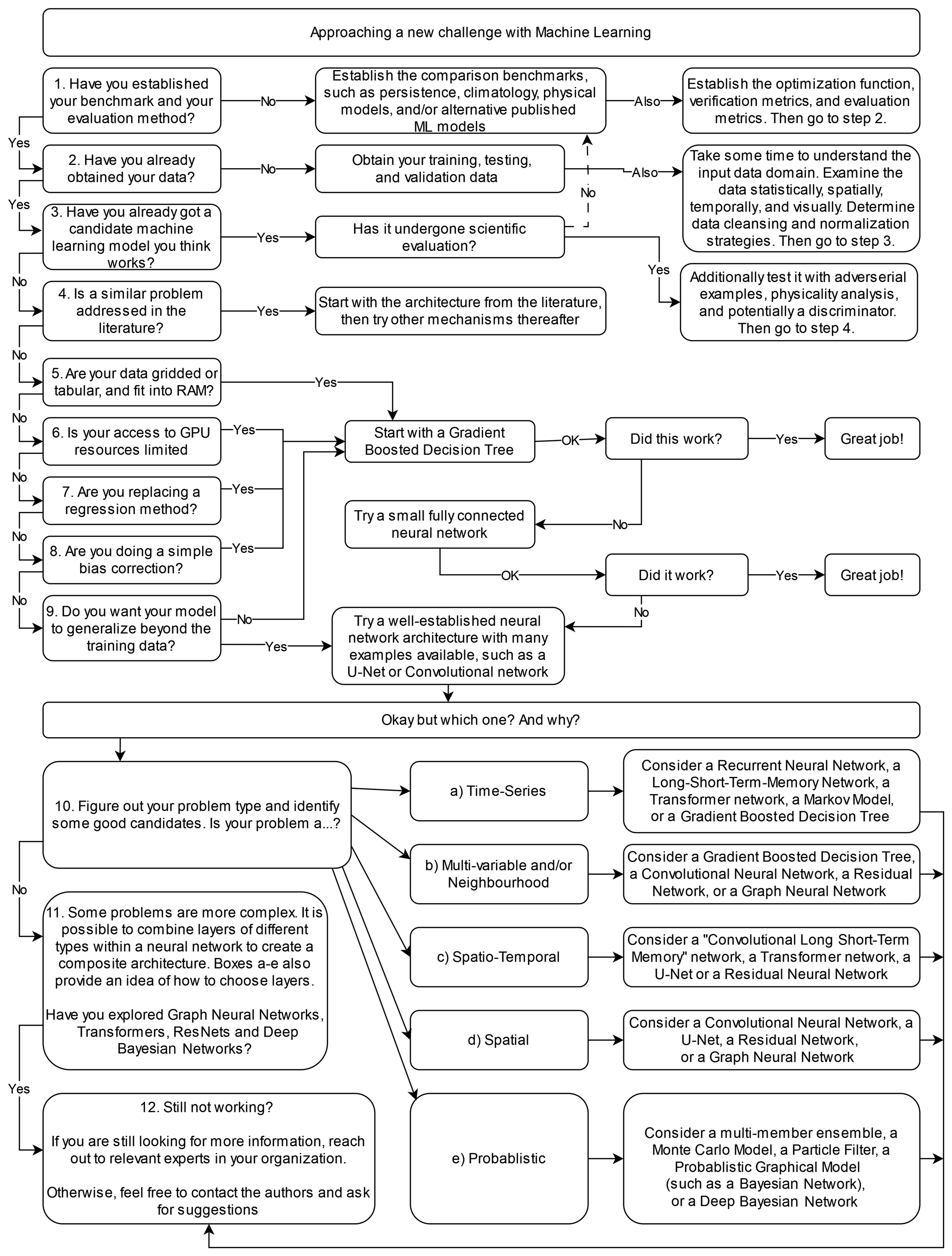
Figure 2A methodological flowchart illustrating a suggested approach to applying ML to a research problem.
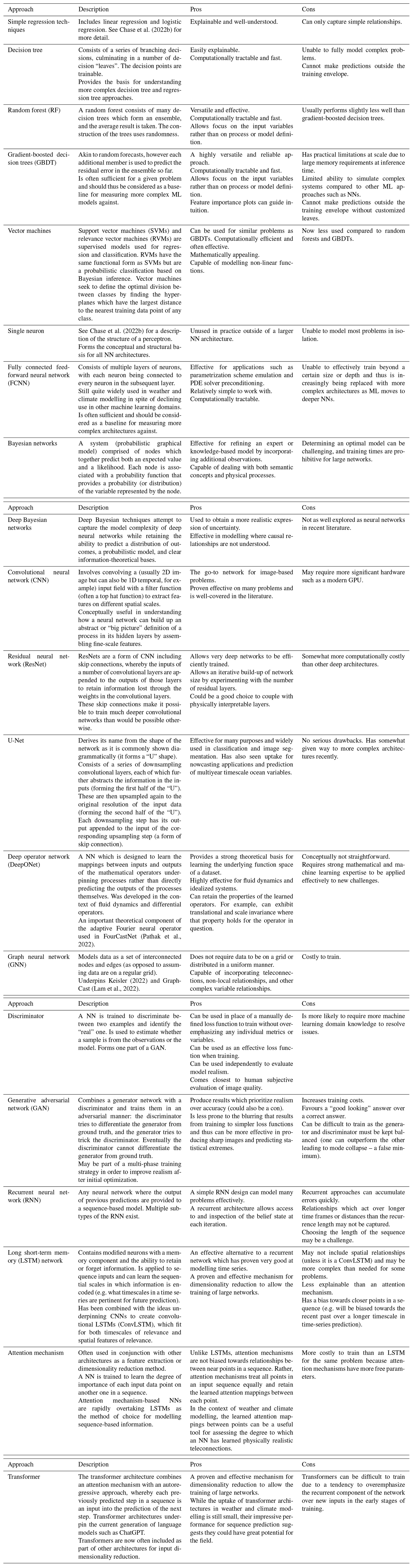
The flowchart presented in Fig. 2 provides an overview of methodological steps that can be taken when using ML to solve a problem; however it does not give much insight into the pros and cons of the common ML architectures available and used in the literature. Table 1 provides a brief summary of the major ML architectures and algorithms used by the studies cited in this review and gives a short note on some of their pros and cons. This table is not exhaustive, and readers are strongly encouraged to use it as a starting point for further exploration rather than a definitive guide. The relative strengths and weakness of each ML architecture can be subtle and highly dependent on the use case, their application, and their tuning. Establishing a good understanding of the ML architecture being used is a critical step for any scientist intending to delve into ML modelling. Interested readers should also refer to Chase et al. (2022b), where a similar table is presented that covers a wider variety of traditional methods but fewer neural network approaches.
An increasingly diverse array ML architectures are being applied to an ever-growing variety of challenges. These architectures all have sub-variants and ancestor architectures which may not be represented, all of which may be found to be of use for weather and climate modelling applications. Other concerns, such as data normalization†, training strategies, and capturing physicality, become as relevant as the choice of architecture once a certain level of performance is achieved.
Figure 3 shows a summary of the ML architectures and algorithms used by the studies cited in this review, including the number of times each architecture is used. It can be seen from this that the two most frequently used general categories of architecture are fully connected NNs (FCNNs) and convolutional NNs (CNNs) of various sub-types.
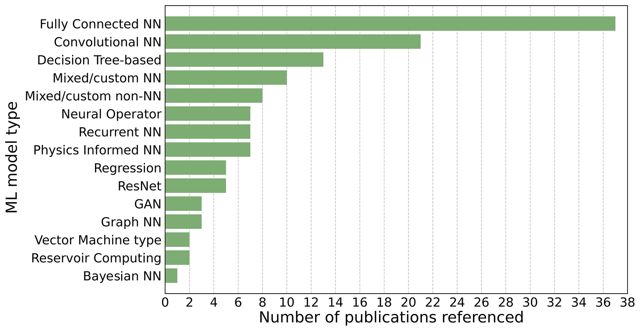
Figure 3A count of the ML architectures and algorithms used by the studies cited in this review. As with Fig. 1, this figure includes all references from this review except for seminal ML papers that are on new ML methods (e.g. foundational ML papers), review papers, any paper cited that concerns a topic which is out of scope (e.g. nowcasting), and any other paper which does not present a new method directly applicable to weather and climate modelling. The full table of citations is provided in Appendix A.
Table 1A summary of major ML architectures and algorithms used by the studies cited in this review. Interested readers should also refer to Chase et al. (2022b) where a similar table is presented that covers a wider variety of traditional methods but fewer neural network approaches. See Appendix B for definitions of terms used in this table.
However some of the most significant recent research findings come from new architectures which by definition cannot have wide adoption yet (these are grouped under the “mixed/custom NN” category in Fig. 3).
In some cases, little justification is given for the ML architecture used in a study, and readers are therefore cautioned against using the relative popularity of a particular ML architecture in the literature as a guide for its suitability for a given task.
Furthermore, ML models increasingly use a mix of different algorithms and architectures. For example, a common combination is fully connected NN layers, convolutional NN layers, and long short-term memory (LSTM†) layers. For the purposes of Fig. 3, the authors have endeavoured to categorize the ML architectures used in the studies in this review as accurately as possible, with complex architectures being placed in the “mixed/custom NN” category; however where an architecture was mostly but not entirely aligned with a single category, it was placed in that category. For example, an LSTM model with a small number of feed-forward layers would be categorized as a recurrent neural network† (RNN). Since many contemporary ML models combine multiple architectural elements and algorithms into the one model, it is somewhat of an oversimplification to consider each of these in isolation, and while starting with a simple model design with a limited selection of layer types is advisable to aid interpretability, there is no reason they cannot be combined or used in conjunction with each other if this improves the performance of the model.
Adapting, optimizing, and debugging issues with machine learning systems can be very complex (especially so for large NNs) and is likely to require both machine learning expertise and domain knowledge (i.e. scientific knowledge). XGBoost† provides the ability to generate a chart showing the importance of the features in the model, which can be very helpful. Shapley additive explanations (Lundberg and Lee, 2017) can provide insights into feature importance for any model including NNs.
Subgrid-scale processes in numerical weather and climate models are typically represented via a statistical parameterization of what the macroscopic impacts of the process would be on resolved processes and parameters. These are commonly referred to as parameterization schemes and can be very complex and relatively computationally costly. For example, in the European Centre for Medium-Range Weather Forecast's (ECMWF) Integrated Forecasting System (IFS) model they account for about a third of the total computational cost of running the model (Chantry et al., 2021b). They also require some understanding of the underlying unresolved physical processes. Examples of subgrid-scale processes which are currently typically parameterized in operational systems include gravity wave drag, convection, radiation, subgrid-scale turbulence, and cloud microphysics. As additional complexity (for example representation of aerosols, atmospheric chemistry, and land surface processes) is added to numerical models, the computational cost will only increase.
ML presents an alternative approach to representing subgrid-scale processes, either by emulating the behaviour of an existing parametrization scheme, by emulating the behaviour of sub-components of the scheme, by replacing the current scheme or sub-component entirely with an ML-based scheme, or by replacing the aggregate effects of multiple parametrization schemes with a single ML model. ML emulation of existing schemes or sub-components has the advantage of maintaining the status quo within the model; no or minimal re-tuning of the model should be required since the ML emulation is trained to replicate the results of an already-tuned-for scheme. Because of this, the main benefit of this approach is that it reduces the computational cost of running the parametrization scheme. On the other hand, the full replacement of an existing parameterization scheme or sub-component with an ML alternative has the potential to be both computationally cheaper and also an improvement over the preceding scheme.
In the following subsections, a review of the literature on aspects of ML for the parametrization and emulation of subgrid-scale processes is presented.
3.1 Early work on ML parametrization and ML emulations
A popular target for applying ML in climate models is radiative transfer since it is one of the more computationally costly components of the model. As such, many early examples of the use of ML in subgrid parametrization schemes focus on aspects of this physical process. Chevallier et al. (1998) trained NNs to represent the radiative transfer budget from the top of the atmosphere to the land surface, with a focus on application in climate studies. They incorporated the information from both line-by-line and band models in their training to achieve competitive results against both benchmarks. Their NNs achieved accuracies comparable to or better than benchmark radiative transfer models of the time while also being much faster computationally.
In contrast to the ML-based scheme developed by Chevallier et al. (1998), which could be considered an entirely new parametrization scheme, Krasnopolsky et al. (2005) used NNs to develop an ML-based emulation of the existing atmospheric longwave radiation parametrization scheme in the NCAR Community Atmospheric Model (CAM). The authors demonstrated speedups with the NN emulation of 50–80 times the original parameterization scheme.
The emulation of existing schemes has since then become a popular method for achieving significant model speedups. For example, Gettelman et al. (2021) investigated the differences between a general circulation model (GCM) with the warm rain formation process replaced with a bin microphysical model (resulting in a 400 % slowdown) and one with the standard bulk microphysics parameterization in place. They then replaced the bin microphysical model with a set of NNs designed to emulate the differences observed and showed that this configuration was able to closely reproduce the effects of including the bin microphysical model, without any of the corresponding slowdown in the GCM.
3.2 ML for coarse graining
Coarse graining involves using higher-resolution model or analysis data to map the relationship between smaller-scale processes and a coarser grid resolution. It can be used to develop parameterization schemes without explicitly representing the physics of smaller-scale processes.
This has proven to be a popular method for developing ML-based parametrization schemes. Brenowitz and Bretherton (2018) used a near-global aquaplanet simulation run at 4 km grid length to train an NN to represent the apparent sources of heat and moisture averaged onto 160 km2 grid boxes. They then tested this scheme in a prognostic single-column model and showed that it performed better than a traditional model in matching the behaviour of the aquaplanet simulation it was trained on. Brenowitz and Bretherton (2019) built on this work by training their NN on the same global aquaplanet 4 km simulation but then embedded this scheme within a coarser-resolution (160 km2) global aquaplanet GCM. Embedding NNs within GCMs is challenging because feedbacks between NN and GCM components can cause spatially extended simulations to become dynamically unstable within a few model days. This is due to the inherently chaotic nature of the atmosphere in the GCM responding to inputs from the NN which cause rapidly escalating dynamical instabilities and/or violate physical conservation laws. The authors overcame this by identifying and removing inputs into the NN which were contributing to feedbacks between the NN and GCM (Brenowitz et al., 2020a) and by including multiple time steps in the NN training cost function. This resulted in stable simulations which predicted the future state more accurately than the coarse-resolution GCM without any parametrization of subgrid-scale variability; however the authors do observe that the mean state of their NN-coupled GCM would drift, making it unsuitable for prognostic climate simulations.
Rasp et al. (2018) trained a deep NN† to represent all atmospheric subgrid processes in an aquaplanet climate model by learning from a multiscale model in which convection was treated explicitly. They then replaced all subgrid parameterizations in an aquaplanet GCM with the deep NN and allowed it to freely interact with the resolved dynamics and the surface-flux scheme. They showed that the resulting system was stable and able to closely reproduce not only the mean climate of the cloud-resolving simulation but also key aspects of variability in prognostic multiyear simulations. The authors noted that their decision to use deep NNs was a deliberate one because they proved more stable in their prognostic simulations than shallower NNs, and they also observed that larger networks achieved lower training losses. However, while Rasp et al. (2018) were able to engineer a stable model that produced results close to the reference GCM, small changes in the training dataset or input and output vectors quickly led to the NN producing increasingly unrealistic outputs, causing model blow-ups (Rasp, 2020). Consistent with this, Brenowitz and Bretherton (2019) report that they were unable to achieve the same improvements in stability with increasing network layers found by Rasp et al. (2018).
3.3 Overcoming instability in ML emulations and parametrizations
O'Gorman and Dwyer (2018) tackled the instabilities observed in NN-based approaches to subgrid-scale parameterization by employing an alternative ML method: random forests (RFs; Breiman, 2001; Hastie et al., 2009). The authors trained a RF to emulate the outputs of a conventional moist convection parametrization scheme. They then replaced the conventional parameterization scheme with this emulation within a global climate model and showed that it ran stably and was able to accurately produce climate statistics such as precipitation extremes without needing to be specially trained on extreme scenarios. RFs consist of an ensemble of DTs, with the predictions of the RF being the average of the predictions of the DTs which in turn exist within the domain of the training data. RFs thus have the property that their predictions cannot go outside of the domain for their training data, which in the case of O'Gorman and Dwyer (2018) ensured that conservation of energy and non-negativity of surface precipitation (both critically important features of the moist convection parametrization scheme) were automatically achieved. A disadvantage of this method, however, is that it requires considerable memory when the climate model is being run to store the tree structures and predicted values which make up the RF.
Yuval and O'Gorman (2020) extended on the ideas in O'Gorman and Dwyer (2018), switching from emulation of a single parametrization scheme to emulation of all atmospheric subgrid processes. They trained a RF on a high-resolution 3D model of a quasi-global atmosphere to produce outputs for a coarse-grained version of the model and showed that at coarse resolution the RF can be used to reproduce the climate of the high-resolution simulation, running stably for 1000 d.
There are some drawbacks to a RF approach compared to an NN approach, however, namely that NNs may provide the possibility for greater accuracy than RFs and also require substantially less memory when implemented. Given that GCMs are already memory intensive this can be a limiting factor in the practical application of ML parametrization schemes. Furthermore, there is the potential to implement reduced precision NNs on GPUs and central processing units (CPUs) which still achieve sufficient accuracy, leading to substantial gains in computational efficiency. Motivated by these considerations, Yuval et al. (2021) trained an NN in a similar manner to how the RF in Yuval and O'Gorman (2020) was trained, using a high-resolution aquaplanet model and aiming to coarse grain the model parameters. They overcame the model instabilities observed to occur in previous attempts to use NNs for this process by wherever possible training to predict fluxes and sources and sinks (as opposed to the net tendencies predicted by the RF in Yuval and O'Gorman, 2020), thus incorporating physical constraints into the NN parametrization. The authors also investigated the impact of reduced precision in the NN and found that it had little impact on the simulated climate.
3.4 From aquaplanets to realistic land–ocean simulations
All of the studies discussed in this section so far which were tested in a full GCM have used aquaplanet simulations. Han et al. (2020) broke away from this trend by developing a residual NN† (ResNet)-based parametrization scheme which emulated the moist physics processes in a realistic land–ocean simulation. Their emulation reproduced the characteristics of the land–ocean simulation well and was also stable when embedded in single-column models.
Mooers et al. (2021) represent a subsequent example of an ML emulation of atmospheric fields with realistic geographical boundary conditions, where the authors developed feed-forward NNs to super-parametrize subgrid-scale atmospheric parameters and forced a realistic land surface model with them. Super-parametrization is distinct from traditional parameterization in that it relies on solving (usually simplified) governing equations for subgrid-scale processes rather than heuristic approximations of these processes. They employed automated hyperparameter† optimization† to investigate a range of neural network architectures across ∼ 250 trials and investigated the statistical characteristics of their emulations. While the authors found that their NNs had a less good fit in the tropical marine boundary layer, attributable to the NN struggling to emulate fast stochastic signals in convection, they also reported good skill for signals on diurnal to synoptic timescales.
Brenowitz et al. (2022) sought to address the challenge of emulating fast processes. They used FV3GFS (Zhou et al., 2019; Harris et al., 2021; a compressible atmospheric model used for operational weather forecasts by the US National Weather Service) with a simple cloud microphysics scheme included to generate training data and used this to train a selection of ML models to emulate cloud microphysics processes, including fast phase changes. They emulated different aspects of the microphysics with separate ML models chosen to be suitable to each task. For example, simple parameters were trained with single-layer NNs, while parameters which are more complex spatially were trained with RNNs (e.g. rain falls downwards and not upwards, so it is sequential in time steps through the atmosphere – a feature which can be represented by an RNN). They then embedded their ML emulation in FV3GFS. They found that their combined ML simulation performed skilfully according to their chosen metrics but had excessive cloud over the Antarctic Plateau.
All of these studies, however, did not test their parameterizations in prognostic long-term simulations.
3.5 Testing with prognostic long-term simulations
A barrier to achieving stable runs with minimal model drift with ML components is the fact that generic ML models are not designed to conserve quantities which are required to be conserved by the physics of the atmosphere and ocean. Beucler et al. (2019) proposed and tested two methods for imposing such constraints in an NN model: (1) constraining the loss function or (2) constraining the architecture of the network itself. They found that their control NN with no physical constraints imposed performed well but did so by breaking conservation laws, bringing into question the trustworthiness of such a model in a prognostic setting. Their constrained networks did, however, generalize better with unforeseen conditions, implying they might perform better under a changing climate than unconstrained models.
Chantry et al. (2021b) trained an NN to emulate the non-orographic gravity wave drag parameterization in the ECMWF IFS model (specifically cycle 45R1; ECMWF, 2018) and were able to run stable, accurate simulations out to 1 year with this emulation coupled to the IFS. While the authors note that RFs have been shown to be more stable (e.g. O'Gorman and Dwyer, 2018, and Yuval and O'Gorman, 2020, as described above, and Brenowitz et al., 2020b), they chose to focus on NNs since they have lower memory requirements and therefore promise better theoretical performance. The authors assessed the performance of their emulation in a realistic GCM by coupling the NN with the IFS, replacing the existing non-orographic gravity wave drag scheme, and performed 120 h, 10 d, and 1-year forecasts at ∼ 25 km resolution in a variety of model configurations. The authors showed that their emulation was able to run stably when coupled to the IFS for seasonal timescales, including being able to reproduce the descent of the quasi-biennial oscillation (QBO). Interestingly, while the authors initially aimed to ensure momentum conservation in a manner similar to Beucler et al. (2021), they found that this constraint led to model instabilities and that a better result was achieved without it. One possible explanation for this is that Beucler et al. (2021) assessed their NNs in an aquaplanet setting. Nonetheless, Chantry et al. (2021b) noted that since their method was not identical to Beucler et al. (2021), improved stability could potentially be achieved by following their method more precisely. The computational cost of the NN emulation developed by Chantry et al. (2021b) was found to be similar to that of the existing parametrization scheme when run on CPUs but was faster by a factor of 10 when run on GPUs due to the reduction in data transmission bottlenecks.
The first study to successfully run stable long-term climate simulations with ML parametrizations was X. Wang et al. (2022), who extended on the work of Han et al. (2020) by constructing a ResNet to emulate moist physics processes. They used the residual connections from Han et al. (2020) to construct NNs with good non-linear fitting ability and filtered out unstable NN parametrizations using a trial-and-error analysis, resulting in the best ResNet set in terms of accuracy and long-term stability. They implemented this scheme in a GCM with realistic geographical boundary conditions and were able to maintain stable simulations for over 10 years in an Atmospheric Model Intercomparison Project (AMIP)-style configuration. This was more akin to a hybrid ML–physics-based model than a traditional GCM with ML-based parametrization because rather than embedding the ResNet in the model code, the authors used an NN–GCM coupling platform through which the NNs and GCMs could interact through data transmission. This is in contrast to the approach employed in the Physical-model Integration with Machine Learning (https://turbo-adventure-f9826cb3.pages.github.io, last access: 7 February 2023) (PIML) project and Infero (https://infero.readthedocs.io/en/latest/, last access: 7 February 2023), which are both described in Sect. 3.11. One advantage to this approach noted by the authors is that it allows for a high degree of flexibility in the application of the ML component; however it is likely to be less efficient than a fully embedded ML model due to the potential for data transmission bottlenecks.
3.6 Training with observational data
An alternative to using more complex and/or higher-resolution models for training data is to train using direct observational data. For example, Ukkonen and Mäkelä (2019) used reanalysis data from ERA5 and lightning observation data to train a variety of different types of ML models to predict thunderstorm occurrence; this was then used as a proxy to trigger deep convection. ML models assessed were logistic regression, RFs, GBDTs, and NNs, with the final two showing a significant increase in skill over convective available potential energy (CAPE; a standard measure of potential convective instability). One of the challenges of accurately reproducing the large-scale effects of convection is correctly identifying when deep convection should occur within a grid cell. The authors proposed that an ML model such as those they assessed could be used as the “trigger function” which activates the deep convection scheme within a GCM.
3.7 ML for super-parameterization
Revisiting the topic of super-parametrized subgrid-scale processes introduced above, the use of ML for this approach was investigated in depth by Chattopadhyay et al. (2020). The authors introduced a framework for an NN-based super-parametrization and compared the performance of this method against an NN-based traditional parametrization (i.e. based on heuristic approximations of subgrid-scale processes) and direct super-parameterization (i.e. explicitly solving for the subgrid-scale processes) in a chaotic Lorenz 96 (Lorenz, 1996) system that had three sets of variables, each of a different scale. They found that their NN-based super-parameterization outperformed the direct super-parameterization in terms of computational cost and was more accurate than the NN-based traditional parametrization. The NN-based super-parameterization showed comparable accuracy to the direct super-parameterization in reproducing long-term climate statistics but was not always comparable for short-term forecasting.
3.8 Stochastic parametrization schemes
A more recent approach to the representation of subgrid-scale processes is via stochastic parameterization schemes, which can represent uncertainty within the scheme. There has been less focus on replacing these schemes with ML alternatives than with non-stochastic schemes; however some progress has been made. Krasnopolsky et al. (2013) used an ensemble of NNs to learn a stochastic convection parametrization from data from a high-resolution cloud resolving model. In this case, the stochastic nature of the parametrization was captured by the ensemble of NNs. Gagne et al. (2020b) took a different approach, investigating the utility of generative adversarial networks† (GANs) for stochastic parametrization schemes in Lorenz 96 (Lorenz, 1996) models. In this case, the GAN learned to emulate the noise of the scheme directly rather than implicitly representing it with an ensemble. They described the effects of different methods to characterize input noise for the GAN and the performance of the model at both weather and climate timescales. The authors found that the properties of the noise influenced the efficacy of training. Too much noise resulted in impaired model convergence and too little noise resulted in instabilities within the trained networks.
3.9 ML parametrization and emulation for land, ocean, and sea ice models
Models of the atmosphere make up one component of the Earth system; however for timescales beyond a few days, simulating other components of the Earth system becomes increasingly important to maintain accuracy. The components which are most often included in coupled Earth system models in addition to the atmosphere are the ocean, sea ice, and the land surface. Reflective of this, ML approaches to the parameterization of subgrid-scale processes are not limited to the atmosphere, and progress has been made in the use of ML for land, ocean, and sea ice models as well.
On the ocean modelling front, Krasnopolsky et al. (2002) presented an early application of NN for the approximation of seawater density, the inversion of the seawater equation of state, and an NN approximation of the non-linear wave–wave interaction. More recently, Bolton and Zanna (2019) investigated the utility of convolutional neural networks (CNNs) for parametrizing unresolved turbulent ocean processes and subsurface flow fields. Zanna and Bolton (2020) then investigated both relevance vector machines† (RVMs) and CNNs for parameterizing mesoscale ocean eddies. They demonstrated that because RVMs are interpretable, they can be used to reveal closed-form equations for eddy parameterizations with embedded conservation laws. The authors tested the RVM and CNN parameterizations in an idealized ocean model and found that both improved the statistics of the coarse-resolution simulation. While the CNN was found to be more stable than the RVM, the advantage of the RVM was the greater interpretability of its outputs. Finally, Ross et al. (2023) developed a framework for benchmarking ML-based parametrization schemes for subgrid-scale ocean processes. They used CNNs, symbolic regression, and genetic programming methods to emulate a variety of subgrid-scale forcings including measures of potential vorticity and velocity, and developed a standard set of metrics to evaluate these emulations. They found that their CNNs were stable and performed well when implemented online but generalized poorly to new regimes.
Focusing instead on sea ice, Chi and Kim (2017) assessed the ability of two NN models: a fully connected NN and an LSTM to predict Antarctic sea ice concentration up to a year in advance. Their ML models outperformed an autoregressive model comparator and were in good agreement with observed sea ice extent. Andersson et al. (2021) improved upon this work with their model IceNet, a U-Net ensemble model which produced probabilistic Arctic sea ice concentration predictions to a 6-month lead time. The authors compared IceNet to the SEAS5 dynamical sea ice model (Johnson et al., 2019) and showed an improvement in the accuracy of a binary classification of ice/no ice for all lead months except the first month. Horvat and Roach (2022) used ML to emulate a parameterization of wave-induced sea ice floe fracture they had developed previously, in order to reduce the computational cost of the scheme. When embedded in a climate simulation, their ML scheme resulted in an overall categorical accuracy (accounting for the fact that it was only called where needed) of 96.5 %. However the authors did note that since their ML scheme was trained on present-day sea ice conditions, it may have reduced success under different climate scenarios, and they recommend retraining using climate model sea ice conditions to account for this. Rosier et al. (2023) developed MELTNET, an ML emulation of the ocean-induced ice shelf melt rates in the NEMO ocean model (Gurvan et al., 2019). MELTNET consisted of a melt rate segmentation task, followed by a denoising autoencoder† network which converted the discrete labelled melt rates to a continuous melt rate. The authors demonstrated that MELTNET generalized well to ice shelf geometries outside the training set and outperformed two intermediate-complexity melt rate parameterizations, even when parameters in those models were tuned to minimize any misfit for the geometries used. Given the computational cost of sea ice parametrizations is relatively high for the timescales on which sea ice evolution is important (namely, seasonal to climate timescales) and given the promising results in emulating these parametrizations demonstrated in the literature, ML-based emulation of these schemes is a strong candidate for inclusion into future dynamical coupled modelling systems.
Finally, considering Earth's surface, most of the focus of ML innovations in this context has been on land use classification (e.g. Carranza-García et al., 2019; Digra et al., 2022) and crop modelling (e.g. Virnodkar et al., 2020; Zhang et al., 2023). The rate of publication of ML applications for land surface models has been slower; however there has nonetheless been steady progress in this space in recent years. Pal and Sharma (2021) presented a review of the use of ML in land surface modelling which provides an excellent primer of the state of the field to that point. They include in their review an overview of land surface modelling components and processes before reviewing the literature on the use of ML to represent them. They separate their review into attempts to predict and parametrize different variables or aspects of the model, including evapotranspiration (Alemohammad et al., 2017; Zhao et al., 2019; Pan et al., 2020), soil moisture (Pelissier et al., 2020), momentum and heat fluxes (Leufen and Schädler, 2019), and parameter estimation and uncertainty (Chaney et al., 2016; Sawada, 2020; Dagon et al., 2020). They also provide a useful summary of the ML architectures that have been used in the publications they discuss. More recently, He et al. (2022) developed a hybrid approach to modelling aspects of the land surface, where a traditional land surface model was used to optimize selected vegetation characteristics, while a coupled ML model simulated a corresponding three-layer soil moisture field. The estimated evapotranspiration from this hybrid model was compared to observations, and it was found that it performed well in vegetated areas but underestimated the evapotranspiration in extreme arid deserts. The ready application of ML to aspects of land surface modelling and the relative sparsity of publications in this space suggest that it is a fertile domain for further research and development.
3.10 ML for representing or correcting a sub-component of a parametrization scheme
An alternative method to replacing or emulating an entire parametrization scheme or schemes with ML is to target the most costly or troublesome sub-components of the scheme, and either replace those or make corrections to them.
Ukkonen et al. (2020) trained NNs to replace gas optics computations in the RTE-RRTMGP (Radiative Transfer for Energetics – Rapid Radiative Transfer Model for General Circulation Model Applications – Parallel; Pincus et al., 2019) scheme. The NNs were faster by a factor of 1–6, depending on the software and hardware platforms used. The accuracy of the scheme remained similar to that of the original scheme.
Meyer et al. (2022) trained an NN to account for the differences between 1D cloud effects in the ECMWF 1D radiation scheme ecRad and 3D cloud effects in the ECMWF SPARTACUS (SPeedy Algorithm for Radiative TrAnsfer through CloUd Sides) solver. The 1D cloud effect solver within ecRad, Tripleclouds, is favoured over the 3D SPARTACUS solver because it is 5 times less computationally expensive. The authors show that their NN can account for differences between the two schemes with typical errors between 20 % and 30 % of the 3D signal, resulting in an improvement in Tripleclouds' accuracy with an increase in runtime of approximately 1 %. By accounting for the differences between SPARTACUS and Tripleclouds rather than emulating all of SPARTACUS, the authors were able to keep Tripleclouds unchanged within ecRad for cloud-free areas of the atmosphere and utilize the NN 3D correction elsewhere.
3.11 Bridging the gap between popular languages for ML and large numerical models
A common toolset for researchers to develop and experiment with different ML approaches to problems is Python libraries, such as PyTorch†, scikit-learn†, TensorFlow†, and Keras†, or other dynamically typed, non-precompiled languages. In contrast, numerical weather models are almost universally written in statically typed compiled languages, predominantly Fortran. To make use of ML emulations or parameterizations in the models thus requires
-
that they be treated as a separate model periodically coupled to the main model (as is done between atmosphere and ocean models for example), or
-
that they be manually re-implemented in Fortran, or
-
that the pre-existing libraries used are somehow made accessible within the model code.
X. Wang et al. (2022; mentioned already above) opted for method 1, developing what could be considered a hybrid ML–physics-based model rather than a traditional GCM with ML-based parametrization. In their study, the authors used an NN–GCM coupling platform through which the NNs and GCMs could interact through data transmission. One advantage to this approach noted by the authors is that it allows for a high degree of flexibility in the application of the ML component; however it is likely to be less efficient than a fully embedded ML model due to the potential for data transmission bottlenecks. This framework was then formalized by Zhong et al. (2023).
There are many examples where method 2 was used, such as Rasp et al. (2018), Brenowitz and Bretherton (2018), and Gagne et al. (2019, 2020a). The obvious disadvantage of this approach is that every change to the ML model being used requires re-implementation in Fortran, and if the aim is to test a suite of ML models, this approach becomes untenable. Furthermore, this approach poses greater technical barriers for scientists developing ML-based solutions for numerical model challenges since they must be sufficiently proficient in Fortran to re-implement models in it rather than using existing user-friendly Python toolkits.
A solution lying somewhere between methods 2 and 3 was developed by Ott et al. (2020), who developed a Fortran–Keras bridge (FKB) library that facilitated the implementation of Keras-like NN modules in Fortran, providing a more modular means to build NNs in Fortran code. This, however, did not fully overcome the drawbacks posed by method 2 on its own; implementation of layers in Fortran is still necessary, and any innovations in the Python modules being used would need to be mirrored in the Fortran library.
Finally, method 3 is being tackled by the Met Office in the PIML (https://turbo-adventure-f9826cb3.pages.github.io/, last access: 7 February 2023) project and by ECMWF with an application called Infero (https://infero.readthedocs.io/en/latest/, last access: 7 February 2023). These projects both seek to develop a framework which can be used by researchers to develop ML solutions to modelling problems in Python and then integrate them directly into the existing codebase of the physical model (e.g. the Unified Model at the UK Met Office). The approach used is to directly expose the compiled code underpinning the Python modules within the physical model code.
The representation and solving of the partial differential equations (PDEs) governing the fluid flow and dynamical processes in the oceans and atmosphere can be considered the backbone of weather and climate models. The solvers used to find solutions to these equations are typically iterative and must solve the dynamics governing equations of their model on every time step and at every grid point. There has been growing interest in using ML to facilitate speedups and computational cost reductions in the preconditioning and execution of these solvers. Preconditioners are used to reduce the number of iterations required for a solver to converge on a solution and usually do so by inverting parts of the linear problem. Many earlier studies focused on using ML to select the best preconditioner and/or PDE solver from a set of possible choices (e.g. Holloway and Chen, 2007; Kuefler and Chen, 2008; George et al., 2008; Peairs and Chen, 2011; Huang et al., 2016; and Yamada et al., 2018). Ackmann et al. (2020) approached the preconditioner part of the system more directly, using a variety of ML methods to directly predict the precondition of a linear solver rather than using a standard preconditioner. Rizzuti et al. (2019) focused on the solver, using ML to apply corrections to a traditional iterative solver for the Helmholtz equation. Going a step further, a number of studies have used ML to replace the linear solver entirely (Ladický et al., 2015; Yang et al., 2016; Tompson et al., 2017). The representation of the fluid equations in a gridded model poses a challenge because of the inability to resolve fine features in their solution. This leads to the use of coarse-grained approximations to the actual equations, which aim to accurately represent longer-wavelength dynamics while properly accounting for unresolved smaller-scale features. Bar-Sinai et al. (2019) trained an NN to optimally discretize the PDEs based on actual solutions to the known underlying equations. They showed that their method is highly accurate, allowing them to integrate in time a collection of non-linear equations in 1 spatial dimension at resolutions 4× to 8× coarser than was possible with standard finite-difference methods.
Building on this, Kochkov et al. (2021) developed an ML-based method to accurately calculate the time evolution of solutions to non-linear PDEs which used grids an order of magnitude coarser than is traditionally required to achieve the same degree of accuracy. They used convolutional NNs to discover discretized versions of the equations (as in Bar-Sinai et al., 2019) and applied this method selectively to the components of traditional solvers most affected by coarse resolution, with each NN being equation-specific. They utilized the property that the dynamics of the PDEs were localized, combined with the convolutional layers of their NN enforcing translation invariance†, to perform their training simulations on small but high-resolution domains, making the training set affordable to produce. An interesting feature of their training approach, which is growing in popularity, was the inclusion of the numerical solver in the training loss function: the loss function was defined as the cumulative pointwise error between the predicted and ground truth values over the training period. In this way, the NN model could see its own outputs as inputs, ensuring an internally consistent training process. This had the effect of improving the predictive performance of the model over longer timescales, in terms of both accuracy and stability. Finally, the authors demonstrated that their models produced generalizable properties (i.e. although the models were trained on small domains, they produced accurate simulations over larger domains with different forcing and Reynolds number). They showed that this generalization property arose from consistent physical constraints being enforced by their chosen method.
An alternative to using ML to discover discretized versions of the PDE equations is to instead use NNs to learn the evolution operator of the underlying unknown PDE, a method often referred to as a DeepONet†. The evolution operator maps the solution of a PDE forwards in time and completely characterizes the solution evolution of the underlying unknown PDE. Because it is operating on the PDE, it is scale invariant† and so bypasses the restriction of other methods that must be trained for a specific discretization or grid scale. Interest in, and the degree of sophistication of, DeepONets has grown rapidly in recent years (e.g. Lu et al., 2019; Wu and Xiu, 2020; Bhattacharya et al., 2020; Li et al., 2020a, b, c; Nelsen and Stuart, 2021; Patel et al., 2021; Wang et al., 2021; Lanthaler et al., 2022) to the point where the method is showing promising speedups: 3× faster than traditional solvers in the case of Wang et al. (2021).
The application of ML to the solving of PDEs and the preconditioning of PDE solvers has been a fruitful avenue of research to date. It has led to innovations which have proven useful even outside of the immediate field (e.g. Pathak et al., 2022, adapted innovations from DeepONets to use in fully ML-based weather models – this is discussed further in the next section). This is likely in part because there are many areas of engineering and science which are active in progressing relevant research, leading to a greater overall pace of innovation. ML-based PDE solvers and preconditioners have not yet been tested in a physical weather and climate model. There are few theoretical reasons this could not occur and, if effective, result in significant computational efficiencies for traditional physical model architectures. This poses an interesting avenue for further research.
The shift from using ML to emulate or replace parametrization schemes to using ML to replace the entire GCM has been made plausible by the increasing volume of training data available. The focus in this section will be on the challenge of completely replacing a GCM with an ML model.
There has been a flurry of activity in the use of ML for nowcasting (e.g. Ravuri et al., 2021); however since the focus of this review is on weather and climate applications, these studies will not be elaborated on.
5.1 Early work – 1D deterministic models
Work on the use of ML to predict chaotic time-domain systems initially focused on 1D problems, including 1D Lorenz systems (e.g. Karunasinghe and Liong, 2006; Vlachas et al., 2018). Of particular interest is Vlachas et al. (2018), who used long short-term memory networks (LSTMs†), which are well-suited to complex time domain problems. Convolutional LSTMs (ConvLSTMs), which combine convolutional layers with an LSTM mechanism, were introduced in the meteorological domain by Shi et al. (2015) for precipitation nowcasting. They have since seen wide adoption in other areas (e.g. Yuan et al., 2018; Moishin et al., 2021; Kelotra and Pandey, 2020). Their success in other domains suggests that revisiting their utility for weather and climate modelling could be worthwhile.
5.2 Moving to spatially extended deterministic ML-based models
Replacing a GCM entirely with an ML alternative was first suggested and tested in a spatially resolved global configuration by Dueben and Bauer (2018), although for this study they only sought to predict a single variable (geopotential height at 500 hPa) on a 6∘ grid. Scher (2018) trained a CNN to predict the next model state of a GCM based on the complete state of the model at the previous step (i.e. an emulator of the GCM). Since this work was intended to be a proof of concept, the authors used a highly simplified GCM with no seasonal or diurnal cycle, no ocean, no orography, a resolution of ∼ 625 km in the horizontal, and 10 vertical levels. Nonetheless, their ML model showed impressive capabilities; it was able to predict the complete model state several time steps ahead and when run in an iterative way (i.e. by feeding the model outputs back as new inputs) was able to produce a stable climate run with the same climate statistics as the GCM, with no long-term drift (even though no conservation properties were explicitly built into the CNN). Scher and Messori (2019) then extended on this but continued the proof-of-concept approach. They investigated the ability of NNs to make skilful forecasts iteratively a day at a time to a lead time of a few days for GCMs of varying complexity and explored a combination of other factors, including number of training years, the effects of model retuning, and the impact of a seasonal cycle on NN model accuracy and stability.
Weyn et al. (2019) aimed to predict a limited number of variables, focusing on the NWP to medium-range time domain. They trained a CNN to predict 500 hPa geopotential height and 300 to 700 hPa geopotential thickness over the Northern Hemisphere to up to a 14 d lead time, showing better skill out to 3 d than persistence†, climatology†, and a dynamics-based barotropic vorticity model but not better than an operational full-physics weather prediction model.
Weyn et al. (2020) then improved on this significantly, with a deep U-Net-style CNN trained to predict four variables (geopotential height at 500 and 1000 hPa, 300 to 700 hPa geopotential thickness, and 2 m temperature) globally to a 14 d lead time. A major innovation in this study was their use of a cubed-sphere grid, which minimized distortions for planar convolution algorithms while also providing closed boundary conditions for the edges of the cube faces. Additionally, they extended their previous work to include sequence prediction techniques, making skilful predictions possible to longer lead times. Their improved model outperformed persistence and a coarse-resolution comparator (a T42 spectral resolution version of the ECMWF IFS model, with 62 vertical levels and ∼ 2.8∘ horizontal resolution) to the full 14 d lead time but was not as skilful as a higher-resolution comparator (a T63 spectral resolution version of the IFS model with 137 vertical levels and ∼ 1.9∘ horizontal resolution) or the operational sub-seasonal-to-seasonal (S2S) version of the ECMWF IFS.
Clare et al. (2021) tackled a short fall of many of the ML weather and climate models developed to this point, namely that most were deterministic, limiting their potential utility. To address this, they trained an NN to predict full probability density functions of geopotential height at 500 hPa and temperature at 850 hPa at 3 and 5 d lead times, producing a probabilistic forecast which was comparable in accuracy to Weyn et al. (2020).
Choosing to focus on improved skill rather than the question of probabilistic vs. deterministic models, Rasp and Thuerey (2021) developed a ResNet model trained to predict geopotential height, temperature, and precipitation to a 5 d lead time and assessed it against the same set of physical models as Weyn et al. (2020). Their model was close to being as skilful as the T63 spectral resolution version of the IFS model, and had better skill to the 5 d lead time than Weyn et al. (2020).
Keisler (2022) took an ambitious step forward, training a graph neural network† (GNN) model to predict 6 physical variables on 13 atmospheric levels on a 1∘ horizontal grid, which the author claims is ∼ 50–2000 times larger than the number of physical quantities predicted by the models in Rasp and Thuerey (2021) and Weyn et al. (2020). Their model worked by iteratively predicting the state of the six variables 6 h into the future (i.e. the output of each model time step was the input into the next time step) to a total lead time of 6 d. The authors showed that their model outperformed both Rasp and Thuerey (2021) and Weyn et al. (2020) in the variables common to all three studies. They suggested that the gain in skill seen over previous studies was due to the use of more channels† of information, as well as the higher spatial and temporal resolution of their model. Finally, they showed that their model was more skilful than NOAA's Global Forecast System (GFS) physical model to 6 d lead time but not as skilful as ECMWF IFS.
Lam et al. (2022) also used GNNs to build their ML-based weather and climate model, GraphCast. This model was the most skilful ML-based weather and climate model at the time of writing this review. While the first ML-based weather and climate model to claim to exceed the skill of a numerical model was Pangu-Weather (Bi et al., 2022; described in greater detail in the following subsection), GraphCast exceeded the skill of both the ECMWF deterministic operational forecasting system, HRES, and also Pangu-Weather. Furthermore, Lam et al. (2022) paid particular attention to evaluating their model and HRES against appropriate measures and included existing model assessment scorecards from ECMWF to evaluate them. GraphCast capitalized on the ability of GNNs to model arbitrary sparse interactions by adopting a high-resolution multi-scale mesh representation of the input and output parameters. It was trained on the ECMWF ERA5 reanalysis archive to produce predictions of five surface variables and six atmospheric variables, each at 37 vertical pressure levels, on a 0.25∘ grid. It made predictions on a 6-hourly time step and was run autoregressively to produce predictions to a 10 d lead time. The authors demonstrated that GraphCast was more accurate than HRES on 90.0 % of the 2760 variable and lead time combinations they evaluated.
5.3 Ensemble generation with ML-based models
A common criticism of ML approaches to weather and climate prediction is the difficulty of representing uncertainty and/or the tails of the distribution of predicted parameters. One common method to represent the range of possible outcomes (including extremes) under different sources of uncertainty is through a well-calibrated ensemble of predictions. There are a growing number of examples where ensemble generation is considered, many of which fall into the category of full-model replacement.
Weyn et al. (2021) explored probabilistic ML predictions using an ensemble of NNs similar to the single-member NN described in Weyn et al. (2020). The authors expanded the number of variables predicted from four to six and produced forecasts to a 6-week lead time – considerably longer than any comparable work at the time of writing this review. They considered a variety of initial-condition perturbation strategies and explored the impact of model error by varying the initial values of the model weights during training to create a multi-model ensemble. They used a combination of the multi-model ensemble generation approach and initial-condition perturbations to generate a “grand ensemble” of 320 members. They used established metrics for ensemble performance such as RMSE spread plots and found that the 320-member grand ensemble combining the multi-model ensemble with initial-condition perturbations performed only slightly better than the multi-model ensemble alone at 14 d lead times. The skill of the ensemble mean of the system, a control member, and the full ensemble were assessed against the same metrics from the ECMWF sub-seasonal to seasonal (S2S) prediction system. Their grand ensemble had lower skill than the S2S system at shorter lead times but was comparable in skill at longer lead times. Their skill assessment used standard probabilistic skill measures such as continuous ranked probability score and the ranked probability skill score, which are not present in the other studies discussed in this section. The next major ML model to be tested in an ensemble mode was FourCastNet, presented by Pathak et al. (2022), who leveraged the work on DeepONets described in Sect. 4. In particular, the authors used a type of DeepONet called a Fourier neural operator (FNO). FourCastNet produced predictions of 20 variables (including challenging-to-predict variables such as surface winds and precipitation) on five vertical levels with 0.25∘ horizontal resolution and had competitive skill against the ECMWF IFS for a 1-week lead time. The high horizontal resolution of their model enabled it to resolve extreme events such as tropical cyclones and atmospheric rivers, and the speed of the model facilitated the generation of large ensembles (up to thousands of members).
The authors explored the potential of their ensemble forecasts by generating a 100-member ensemble from initial conditions perturbed with Gaussian random noise. They showed that the FourCastNet ensemble mean had lower RMSE and a higher anomaly correlation coefficient than a single-value prediction at longer lead times (beyond ∼ 3–4 d), although the ensemble mean performed slightly worse than the single-value forecast at shorter lead times. The authors attributed this relative decrease in performance at shorter lead times to the ensemble mean smoothing out fine-scale features. Unfortunately, the authors did not examine the spread of the ensemble with lead time or evaluate the model using probabilistic skill metrics (in contrast to Weyn et al., 2021), and while they did consider the capacity of FourCastNet to predict extremes, they did not do so in an ensemble context.
Hu et al. (2023) improved on the relatively simple ensemble perturbation approach employed by Pathak et al. (2022) in their model, a sliding window (Swin) transformer-based variational recurrent neural network (SwinVRNN). This model combined a Swin transformer recurrent neural network (SwinRNN) predictor with a variational autoencoder perturbation module. The perturbation module learned the multivariate Gaussian distributions of a time-variant stochastic latent variable from the training data. The SwinRNN predictor was deterministic but could be used to generate ensemble predictions by perturbing model features using noise sampled from the distribution learned by the perturbation module. Unlike the approach used by Pathak et al. (2022), this strategy ensured that the perturbations applied at each spatial location in ensemble generation were appropriate for the location and variable in question. Furthermore, the training strategy employed by Hu et al. (2023) accounted for both the error in the deterministic predictions and the error in the learned perturbation distribution, effectively optimizing forecast accuracy and ensemble spread at the same time. The authors assessed both the ensemble spread and ensemble mean accuracy of their model and found that it had a better ensemble spread than simpler alternative ensemble generation strategies. They also found that it had lower latitude-weighted RMSE than the ECMWF IFS to a 5 d lead time for 2 m temperatures and total precipitation. ECMWF data beyond 5 d were not shown, but the SwinVRNN models had latitude-weighted RMSE values lower than a weekly climatology baseline for three of the four variables shown to a 14 d lead time. Bi et al. (2022) achieved a significant milestone with their model Pangu-Weather, the first ML-based model to perform better than the ECMWF IFS to a lead time of 7 d based on RMSE and anomaly correlation coefficient (ACC) across several variables including geopotential height and temperature at 500 hPa. While they did explore the utility of Pangu-Weather for ensemble generation, their approach was more simplistic than that demonstrated by Hu et al. (2023). Pangu-Weather featured two major innovations over previous contributions to this space:
-
It used 3D (latitude, longitude, and height) input grids trained against 3D output grids. This enabled different levels of the atmosphere to share information, which was not possible in FourCastNet in spite of predicting variables on multiple atmospheric levels because the levels were treated independently. In contrast, Pangu-Weather adopted a 3D convolutional method that the authors name the 3D Earth-specific transformer (3DEST), which enabled the flow of information both horizontally and vertically.
-
It was made up of a series of models trained with different prediction time gaps. The motivation for this was that, as noted by the authors, when the goal is to produce forecasts to 5 d (for example) but the time step of the basic forecast model is relatively short (e.g. 6 h), many iterative executions of the model are required, with the errors in each iteration feeding into the next. A shorter model time step results in greater overall errors (due to more iterations being required to reach the final forecast lead time), and a longer model time step reduces this error. Motivated by this, the authors trained several versions of their model to predict different time steps on a single iteration. The overall forecast to a given lead time was then constructed using the longest possible time steps. For example, for a 7 d forecast, a 24 h forecast is iterated seven times, whereas for a 23 h forecast, a 6 h forecast is iterated three times, followed by a 3 h forecast one time, and 1 h forecast two times. The authors noted that this strategy was not effective for multi-week or longer timescales; they reported that training the model with a 28 d time step was difficult, for example, and suggested that more powerful or complex ML methods would be required to achieve this.
As well as the relatively broad measures of RMSE and ACC, the authors assessed the ability of their system to represent the intensity and track of selected tropical cyclones. They found that Pangu-Weather predicted the tracks of the cyclones considered with a high degree of accuracy compared to the ECMWF IFS; however it underestimated cyclone intensity. The authors attributed this to the training data they used (ERA5) also underestimating cyclone intensity. As noted above, the authors also explored the potential for producing useful ensemble forecasts. To assess ensemble predictions, they perturbed the initial state of the system with Perlin noise vectors to produce a 100-member ensemble of forecasts and calculated the RMSE and ACC of the ensemble mean for selected variables. As in Weyn et al. (2021), the authors noted that the ensemble mean forecasts performed worse than a single deterministic forecast for shorter lead times (e.g. 1 d) but better for longer lead times. Unfortunately, as with Pathak et al. (2022), Bi et al. (2022) did not investigate the properties of the spread of the ensemble or assess its skill using standard probabilistic skill metrics, and their approach to ensemble generation was much simpler than that of Hu et al. (2023).
As already mentioned above, the skill of Pangu-Weather was exceeded by GraphCast, although Lam et al. (2022) only assessed GraphCast in a deterministic setting. Nonetheless, there is nothing stopping GraphCast from being used to generate ensemble forecasts in a manner similar to Pangu-Weather. The authors of this review look forward to a more in-depth inter-comparison of the pure ML models in the literature, including an assessment of their performance for ensemble predictions.
Although the ensemble systems presented in Weyn et al. (2021) and Hu et al. (2023) had lower overall accuracy than the other models discussed in this section, they still represented the most comprehensive analysis of the behaviour and performance of ensemble ML models (in terms of considering optimal ensemble perturbation strategies and quantifying the ensemble behaviour) at the time of writing this review. Further investigation into the best methods to generate and evaluate pure ML model ensembles would be a highly beneficial contribution to the field.
5.4 Moving to more extensible models
As the effectiveness of ML approaches are increasingly demonstrated in the literature, additional factors become clear in considering these models for both research and application. In a research setting, the ability to readily perform transfer learning† to new problems and reduce training costs will be significant in supporting adoption by other researchers.
This need for greater flexibility in both the input data sources and predictive outputs of ML weather and climate models was recognized by Nguyen et al. (2023), who developed a transformer-architecture-based ML model called ClimaX. This model was designed as a foundational model, trained initially on datasets derived from the CMIP6 (Eyring et al., 2016) dataset, and able to be readily retrained to specific tasks using transfer learning. The authors demonstrated the skill of ClimaX against simpler ML models, and in some cases a numerical model (ECMWF IFS), for a variety of tasks including weather prediction, sub-seasonal prediction, climate scenario prediction, and climate downscaling. The authors showed that ClimaX was able to make skilful predictions in scenarios unseen during the initial CMIP6 training phase. Furthermore, ClimaX used novel encoding and aggregation blocks in its architecture to enable greater flexibility in the types of variables used for training and to reduce training costs when a large number of different input variables were used.
5.5 Benchmark datasets for ML weather models
Providing open benchmark data for machine learning challenges has been as transformational for the machine learning field as improved algorithms, the publication of papers, or improvements in hardware.
As the interest and activity in the use of ML as a potential alternative to knowledge-based numerical GCMs has grown, the need for consistent benchmarks for the inter-comparison of ML-based models has become increasingly clear. Rasp et al. (2020) addressed this need with the introduction of WeatherBench. On this platform, the authors provided data derived from the ERA5 archive that have been simplified and streamlined for common ML use cases and use by a broad audience. They also proposed a set of evaluation metrics which facilitate direct comparison between different ML approaches and provided baseline scores in these metrics for simple techniques such as linear regression, some deep learning models, and some GCMs. Since the publication of WeatherBench, more benchmark datasets tailored to other domains have been created, including RainBench (de Witt et al., 2020), WeatherBench Probability (Garg et al., 2022), and ClimateBench (Watson-Parris et al., 2022). Weyn et al. (2020) chose datasets and assessment metrics consistent with WeatherBench to facilitate the inter-comparison of results. Rasp and Thuerey (2021) directly used the benchmarks provided by WeatherBench in their assessment. They demonstrated that their model outperformed previous submissions to WeatherBench, highlighting its value as a tool to allow inter-comparability of ML-based weather models. Other examples of studies using WeatherBench data and analysis methods are Clare et al. (2021) and Weyn et al. (2021). The parameters of a good benchmark dataset were further elucidated by Dueben et al. (2022), who provided an overview of the current status of benchmark datasets for ML in weather and climate in use in the research community and provided a set of guidelines for how researchers could build their own benchmark datasets.
At the time of writing this review, assessments of ML-based models had chiefly (but not exclusively) focused on simple statistics like globally averaged RMSE and are not reported in detail to the degree to which they accurately captured specific processes such as cyclone formation, climate drivers such as the El Niño–Southern Oscillation (ENSO), or large-scale structures such as the jet streams. A useful contribution from the scientific community would be to better quantify and articulate a suite of tests and statistics that could form a “report card” to provide better insight into the value of new ML models.
It should also be noted that all of the major milestones and high-profile ML models described in this section so far have relied to some degree or another on reanalysis datasets produced by physics-based models. The provision of higher-resolution and higher-quality open datasets has the potential to drive progress in this area as much as, if not more than, improvements and further research into ML algorithms.
5.6 A hybrid approach
Arcomano et al. (2022) present an approach which straddles the theme of this section and that of the following section (physics-constrained ML models). Following Wikner et al. (2020), they used a numerical atmospheric GCM and a computationally efficient ML method called reservoir computing in a hybrid configuration called combined hybrid-parallel prediction (CHyPP). Their hybrid model is more accurate than the GCM alone for most state variables to a lead time of 7–8 d. They also demonstrate the utility of their hybrid model for climate predictions with a 10-year-long climate simulation, for which they showed that the hybrid model had smaller systematic errors and more realistic variability than the GCM alone.
5.7 ML for predicting ocean variables
More recently, greater attention has been paid to the application of ML to the ocean, particularly for seasonal to multiyear predictions. Initial work in this space focused on directly predicting key indices such as the NINO3.4 index. For example, Ham et al. (2019) trained a CNN to produce skilful ENSO forecasts with a lead time of up to 1.5 years. A limiting factor for the application of ML to ocean variables is the lack of availability of observational data for training. To overcome this, the authors used transfer learning to train their model first on historical simulations and then on a reanalysis from 1871 to 1973. Data from 1984 to 2017 were reserved for validation. Ham et al. (2021) improved on this by including information about the current season in the network inputs as one-hot vectors†. Including this seasonality information led to an overall increase in skill relative to the model in Ham et al. (2019), in particular for forecasts initiated in boreal spring, a season which is particularly difficult to predict beyond.
Kim et al. (2022) improved on the performance of the 2D CNNs used in Ham et al. (2019, 2021) for predicting ENSO by instead using a convolutional LSTM network with a global receptive field†. The move to a larger (global) receptive field for the convolutional layers enabled the network to learn the large-scale drivers and precursors of ENSO variability, and the use of a recurrent† architecture (in this case LSTM) facilitated the encoding of long-term sequential features with visual attention†. This led to a 5.8 % improvement in the correlation coefficient for NINO3.4 index prediction and 13 % improvement in corresponding temporal classification with a 12-month lead time compared to a 2D CNN.
Taylor and Feng (2022) moved from the prediction of indices to spatial outputs, training a U-Net LSTM model on ECMWF ERA5 monthly mean sea surface temperature (SST) and 2 m air temperature data from 1950–2021 to predict global 2D SSTs up to a 24-month lead time. The authors found that their model was skilful in predicting the 2019–2020 El Niño and the 2016–2017 and 2017–2018 La Niñas but not for the 2015–2016 extreme El Niño. Since they did not include any subsurface information in their training data (in contrast to Ham et al., 2019, 2021, who included ocean heat content), they concluded that subsurface information may have been relevant for the evolution of that event.
It is clear from the small number of (but rapidly evolving) studies in this space that there is great promise for the use of ML for the seasonal and multiyear prediction of ocean variables, with many avenues to pursue to achieve potential skill gains.
5.8 ML for climate prediction
The literature on the use of ML for prediction on seasonal to climate timescales is still relatively sparse compared to its use for nowcasting and weather prediction. Some examples have been covered in previous sections, such as Weyn et al. (2021) on sub-seasonal to seasonal timescales in the atmosphere and Ham et al. (2019, 2021), Kim et al. (2022), and Taylor and Feng (2022) on seasonal to multiyear timescales in the ocean. A major cause for this sparsity is that deep learning typically requires large training datasets, and the available observation period for the earth system is too short to provide appropriate training data for seasonal to climate timescales in most applications. On the sub-seasonal to seasonal end, this may be overcome by including more slowly varying fields in the training (e.g. ocean variables), by designing models to learn the underlying dynamics which drive long-term variability, and by including more physical constraints on the models. On the climate end these same methods could be beneficial, as well as transfer learning, as is done in Ham et al. (2019), and data augmentation† techniques. Additionally, interest is increasing in the use of ML to predict weather regimes and large-scale circulation patterns, which may prove beneficial in informing seasonal and climate predictions (Nielsen et al., 2022). Watson-Parris (2021) argued that the differences between NWP to multiyear prediction and climate modelling mean that the ML approaches best suited to each can be very different. This may also help to explain why the rapid pace of advances in ML-based weather models has not translated into a similar trend in climate modelling.
Despite this, with the growing maturity of the field of ML for weather and climate prediction, there is every reason to believe the challenges of prediction on seasonal to climate timescales can be overcome.
As has been briefly touched on in previous sections, a promising and increasingly popular method for improving the performance of ML applications in weather and climate modelling is to include physics-based constraints in the ML model design (e.g. Karpatne et al., 2017; De Bézenac et al., 2017; Beucler et al., 2019; Yuval et al., 2021; Beucler et al., 2021; Harder et al., 2022). This can be done through the overall design and formulation of the model and through the use of custom loss functions which impose physically motivated conservations and constraints.
An excellent review of the possible methods for incorporating physics constraints into ML models for weather and climate modelling, along with 10 case studies of noteworthy applications of these methods, is presented in Kashinath et al. (2021). The scope of Kashinath et al. (2021) is broad and includes studies not applied directly in the context of weather and climate modelling but that are applicable to it. Rather than repeat the total of this summary here, the reader is directed to this review.
A class of physics-leveraged ML which has grown rapidly in popularity is physics-informed neural networks† (PINNs). These are discussed in Kashinath et al. (2021) and have also become a very active area of research since the publication of that review. A more up-to-date review of this class of NNs is presented by Cuomo et al. (2022), along with a review of other related physics-guided ML architectures.
While PINNs are an exciting and promising new NN architecture, they still face some challenges. For example, they have had little success simulating dynamical systems whose solution exhibits multi-scale, chaotic, or turbulent behaviour. S. Wang et al. (2022) attributed this to the inability of PINNs to represent physical causality and developed a solution by re-formulating the loss function of a PINN to explicitly account for physical causality during model training. They demonstrated that this modified PINN was able to successfully simulate chaotic systems such as a Lorenz system and the Navier–Stokes equations in the turbulent regime, something which traditional PINNs were unable to do.
Nonetheless, recent work with PINNs has led to some interesting results for weather and climate simulation: Bihlo and Popovych (2022) used PINNs to solve the shallow-water equations on a rotating sphere, as a demonstration of their utility in a meteorological context, and Fuhg et al. (2022) developed a modified PINN to solve interval and fuzzy partial differential equations, enabling the solving of PDEs including uncertain parameter fields.
Aside from the most active areas of development in the use of ML in weather and climate models discussed in the sections above, there are a few areas of the literature worth mentioning that are adjacent to the main focus of this review. These topics are covered in the following subsections.
7.1 Nudging
Rather than replacing a component or components of a GCM with an ML alternative to gain skill improvements, Watt-Meyer et al. (2021) focused on using corrective nudging to reduce model biases and the errors they can introduce through feedbacks. The authors used RFs to learn bias-correcting tendencies from a hindcast nudged towards observations. They then coupled this RF to a prognostic simulation and attempted to correct the model drift with the learned nudging tendencies. While this simulation ran stably over the year-long test period and showed improvements in some variables, the errors in others were observed to increase. So far studies in this space seem to be limited to Watt-Meyer et al. (2021); however this method seems promising, so hopefully interest in developing this approach further will grow in the future.
7.2 Uncertainty quantification
A common criticism of some ML models such as NNs is that it is difficult to represent the uncertainty of their outputs. Some examples of studies that have sought to overcome this have already been mentioned in Sect. 3.8, and there are other examples in the literature (e.g. Grigo and Koutsourelakis, 2019; Atkinson, 2020; Yeo et al., 2021; O'Leary et al., 2022); however it is nonetheless still a relatively underexplored aspect of ML models for physical systems. Psaros et al. (2022) suggest that this may be because they are also under-utilized within the broader deep learning community, and it is thus a developing field that is not universally trusted and understood yet. They also point out that the physical considerations inherent to ML applied to physical systems often make them more complicated and computationally expensive than standard ML applications, further disincentivizing the inclusion of uncertainty quantification in an already complex problem.
Only recently has attention to this aspect of ML become sufficient to motivate the collection of methods into a consistent framework, a good example of which is the aforementioned Psaros et al. (2022), who presented a comprehensive review of the methods for quantifying uncertainty in NNs and provided a framework for applying these methods.
A related topic which is facing similar challenges is the question of explainability of ML approaches; often there is value in understanding the relative roles and importance of predictors in an ML model or the relative significance of different regions of the predictor data. Flora et al. (2022) provide a good overview of approaches to this and compare their relative drawbacks and benefits.
7.3 Capturing extremes
While there is now an abundance of examples of ML being used for model parameterization schemes, full-model replacement, downscaling, and PDE solvers (much of which is covered in this review), there are relatively few examples which address the question of how well ML approaches can reproduce extreme events and statistics, both in terms of the distribution of values predicted in a single-member (i.e. non-ensemble and non-probabilistic) ML model and in terms of the distribution of predicted outcomes in a probabilistic or ensemble ML model.
Both Pathak et al. (2022) and Bi et al. (2022), introduced in Sect. 5.2, investigated the ability of their models to correctly represent extremes, using a similar approach. They divided their test dataset into 50 percentile bins (distributed logarithmically by Pathak et al., 2022, and linearly by Bi et al., 2022) between the 90th and 99.99th percentiles and computed the relative quantile error between their forecast and ground-truth as a function of lead time. Pathak et al. (2022) note that they set their highest percentile bin at 99.99 % because of the small sample of data points beyond this percentile making a statistically significant analysis difficult. Both Pathak et al. (2022) and Bi et al. (2022) found that their models consistently under-forecast extremes to a greater degree than the ECMWF IFS.
Watson (2022) presents a strong argument for the need for a greater focus on the ability of ML weather and climate models to be able to predict extremes in order for them to meet the needs of users. They present a summary of some examples of ML models which have sought to predict extreme events according to certain return period definitions. The example most relevant for this review is Lopez-Gomez et al. (2023), who used an NN with a custom loss function that preferentially weighted extremes to predict global extreme heat. They found that their custom loss function led to improved representation of the tails of the distribution (i.e. predictions of extreme heat) and, interestingly, did not result in any major loss of performance for the middle of the distribution.
The under-prediction of extremes seen in Pathak et al. (2022) and Bi et al. (2022) is consistent with the findings of Lopez-Gomez et al. (2023), given that they were optimized for predicting extremes. These findings all point to the idea that in order for ML weather and climate models to be able to skilfully predict extreme events, model training regimes, loss functions, and architectures will need to be employed which take into consideration ways to optimize for these regimes.
7.4 Object identification within models
An alternative to achieving greater model accuracy and skill for predicting extremes through increasing the resolution of the entire model grid is to develop techniques to identify critical systems and physical phenomena within the model and to embed higher-resolution temporary subgrids or specialized models within the larger GCM to more accurately simulate those processes. A challenge to overcome to achieve this is automatically identifying key model features since it typically requires a labelled dataset. This requirement can, however, be avoided, and a variety of both supervised and unsupervised machine learning approaches to object detection have been demonstrated in the literature.
Mudigonda et al. (2017) were a relatively early example of the application of ML to this challenge. They investigated the feasibility of using a variety of NN architectures to identify storms, tropical cyclones, and atmospheric rivers within model data with promising results. Prabhat et al. (2021) provided a valuable resource to the community with their development of ClimateNet, a labelled open dataset and ML model for the segmentation and identification of tropical cyclones and atmospheric rivers. This was used by Kapp-Schwoerer et al. (2020) to train an NN to identify and track these extreme events in Community Atmosphere Model 5 (CAM5; Conley et al., 2012) data. O'Brien et al. (2020) considered the need for uncertainty quantification in object identification, using a Bayesian approach to build an atmospheric river detection framework. Finally, Rupe et al. (2023) took a physics-informed approach to object detection, defining “local causal states” using speed-of-light causality arguments to identify regions of organized coherent flow and bypassing the requirement for labelled datasets. They demonstrated the utility of their approach for the unsupervised identification and tracking of hurricanes and other examples of extreme weather events.
While there are unsupervised learning approaches which have shown value for object detection in weather and climate data (e.g. Rupe et al., 2023), a major limitation of this area of research is the shortage of labelled datasets for supervised learning methods, with ClimateNet being an isolated example.
7.5 GPUs and specialized compute resources
GPUs and tensor processing units (TPUs)† are specialized hardware which are well suited to highly parallelizable matrix operations, ideal for solving neural network operations. TPUs have been developed specifically for deep learning applications. Both GPUs and TPUs are likely to be available on many of the next generation of supercomputers, but much of the current Fortran-based numerical weather and climate model infrastructure cannot be run on them in their current state. Data bottlenecks also exist between the GPUs (which have their own on-board memory) and the main memory accessible to the CPU. While efforts are underway to make numerical and climate models better suited to GPUs, for example with the development of LFRic (Adams et al., 2019), the new weather and climate modelling system being developed by the UK Met Office to replace the existing Unified Model (Walters et al., 2017), there is still a long way to go before entire weather and climate models can be reliably run on GPUs or other specialized compute architectures. At the same time, some neural network designs are aimed squarely at the partial differential equation solving at the core of numerical methods. Since neural network evaluation utilizes simpler mathematical operations than current PDE solvers, they offer the prospect of significant computational advantages on non-specialized (i.e. CPU) hardware.
This section provides a brief perspective on weather and climate modelling from the computer science domain and aims to provide the earth system scientist with a short list of the main relevant innovations in computer science. As was noted in Sect. 1, ML models are often regarded as black boxes, largely because of the design of many prominent ML systems. In principle, it is not quite right to refer to the trained model as “a machine learning model”, in the sense that the process of training the model is “machine learning”; once the model is trained it is definable by a set of mathematical equations and coefficients, much like any physical, statistical, or theoretical model. Thus the machine learning refers to the training process, not the model itself. The essence of ML is the level of automation involved. Even in typical ML models such as large NNs, the model architecture is typically specified manually by the data scientist or physical scientist involved. The automated derivation of model architecture and composition is not yet mature for large models, although it is explored through evolutionary programming techniques, whereby the learning of architecture as well as parameterization is automated.
The complex nature of the Earth system means that ML models which seek to emulate it (or sub-components of it) will likely also need to be quite complex and will contain a mixture of ML architectures and algorithms. This is borne out by the increasing degree of complexity and variety seen in the ML models in the literature reviewed in previous sections.
A large degree of the current research focus is on very large or deep NNs which rely both on the universal approximation theorem and practical experimentation to capture a prediction function without needing to explicitly represent the processes being modelled. In a conceptually similar fashion to how a Fourier decomposition can represent any wavelike function, the universal approximation theorem establishes that an NN may approximate any function, subject to its size and the required degree of accuracy (Hornik et al., 1989). Deep learning has been highly effective in approaching many problems, but many limitations are acknowledged, as evidenced by the current widespread focus on trustworthy computing and efforts towards explainable ML systems. Some ML models take a direct approach to modelling the uncertainty of the system being simulated by representing the model state variables as a probability distribution or degree of confidence. Many contemporary weather and climate models derive their probabilistic outputs from an ensemble of perturbed members; however an alternative approach is to represent each part of the belief state† of the model as a distribution or likelihood, built up either empirically or by fitting a Gaussian or other known distribution (e.g. Clare et al., 2021).
A timeline of some key innovations in ML is presented in Fig. 4. The scale of the timeline is broken between 1956 and 1974, and taking that gap in progress into account, it is clear from this visualization that the rate of innovation in ML has increased significantly over the last 35 or so years. This is likely driven by a range of factors including the increasing availability of compute resources suited to ML applications and the explosion of available data for training.
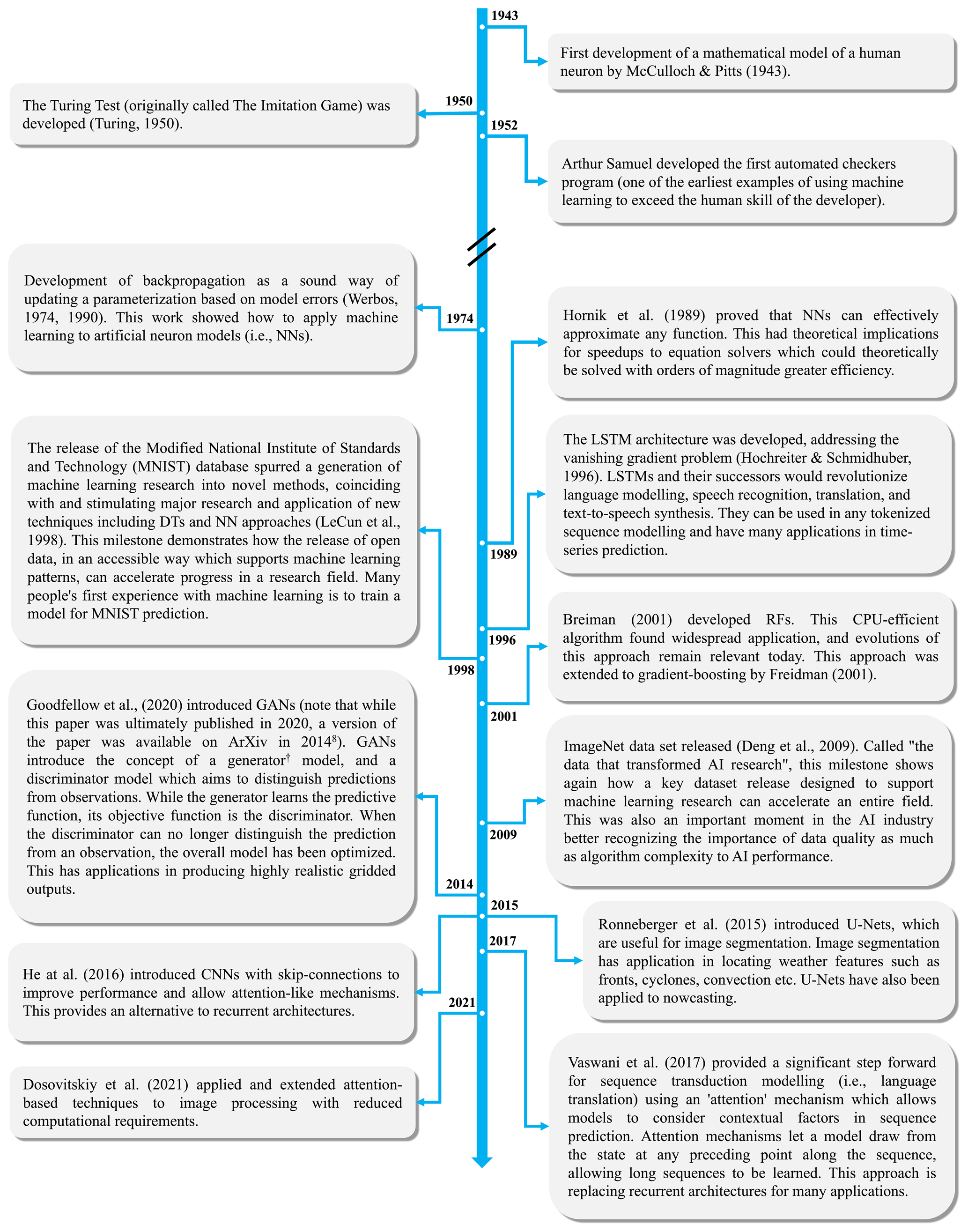
This history shows the degree and rate of research into processing images, text, and other sequences based on the semantic understanding of content but does not demonstrate capturing physical processes as a core element. Advances in the weather and climate modelling domain have a more explicit goal of properly portraying real physical processes. Bringing these concepts together promises to uplift capability in both fields.
A major driver of research into, and improvement in, weather and climate models is increasing the skill of operational forecast systems and increasing the accuracy and trustworthiness of climate projections. Therefore, an important consideration for ML in the context of weather and climate models is the need for it to ultimately be integrated into a complete predictive system with practical applications for forecasting or climate projections.
However the research findings covered in this review, in spite of being compelling, are yet to make major changes to operational modelling systems or standard climate projections.
We have identified three major challenges facing the transition of ML-based innovations into operational settings. Similar challenges are faced in the context of climate projections; however since these are out of the scope for this review, we do not discuss them directly and instead leave them as a topic for other publications.
The first challenge is the need to assess when a research finding is sufficiently compelling and robust to justify integration into established operational systems. Since the major function of operational meteorological services is to inform us of future conditions, largely for managing risk or optimizing benefits, a conservative approach is taken to changing these systems. The utmost premium is put on accuracy, resilience, reliability, and solid scientific foundation, and many novel research findings require extensive further evaluation and development before they can be considered ready for inclusion into operational systems. Understanding when to invest this degree of effort in bringing a research innovation into a major model or scientific configuration upgrade can be difficult.
The second major challenge is establishing the right balance between potentially unwieldy monolithic ML models which predict all variables of interest and many smaller limited-scope models which each focus on predicting one or a small number of variables well. The former option is more similar to current dynamical systems, while the latter option is potentially more easily achievable using an ML approach but risks becoming difficult to manage due to the proliferation of small, separate systems. The early effectiveness of limited-purpose ML models provides the ability to augment existing services without disruption; however aside from the logistical complexity of many small systems, a risk associated with this approach is that inconsistencies between predictions may arise from their independent forecasts, leading to confusion from users and an erosion of trust.
Finally, the third major challenge is how to best monitor and maintain the skill of ML-based systems in a real-time operational context. Explainability of ML systems is an emerging field and is not yet sufficiently mature for application to real-time operational monitoring. Until this changes, the ongoing trustworthiness of operational ML systems will be difficult to demonstrate. Similarly, online learning in ML weather and climate models is not yet a well-explored research area. The use of online learning is likely to be important for operational ML models to be able to develop resiliency and maintain good skill over time, so more work will be needed in this area before these models can see greater uptake in operational systems.
In addition to these major challenges, agencies looking to incorporate ML components into their operational systems must consider
-
the explainability of ML model errors in the case of poor forecasts that may come under scrutiny,
-
that the robustness of ML models to real-time data issues such as data dropouts or input data degradation must be established, and
-
that the lack of infrastructure in these agencies to support ML models in an operational setting will need to be addressed.
Operational development is typically quite incremental, and it is likely that progress will be made in small achievable steps along the evolving technical frontier. However promising and fascinating as a research direction, full-model replacement with ML alternatives is currently not mature enough for an operational setting. Instead, the authors predict that the first types of ML systems to be seen in operations will include parameterization scheme replacements and emulators, solver replacements, super resolution, new approaches to data assimilation of novel observation sources, and both pre- and postprocessing applications (although of course not all of these have been covered in this review).
It is expected that the research into, and application of, ML methods will represent a growing proportion of weather and climate model research, with increasingly sophisticated and skilful model components finding their way into major model releases over the coming years. These components are appealing for both computational and model skill reasons and are expected to be highly promising avenues of research.
Not all papers in this review included a discussion of the ethical considerations associated with using machine learning nor necessarily touched on what constitutes a sufficiently rigorous verification methodology for machine learning models. There is a clear relationship between ethical considerations, the explainability of models, and the rigour of verification applied to ensure that models behave as expected under a variety of conditions (and do not include unexpected behaviours).
While this review paper does not provide an introduction to AI and ML ethics in general, a brief overview of some of the important considerations for the application of ML in the context of weather and climate modelling is provided in this section. Ethical frameworks vary in different cultural and geographical contexts, and for a more general introduction to the ethical considerations surrounding AI and ML, the reader is directed to the paper Recommendations on the Ethics of Artificial Intelligence (United Nations Educational, Scientific and Cultural Organization (UNESCO), 2020).
For ML applied to weather and climate modelling, some considerations to ensure sufficient robustness and reliability include whether
-
testing, training, and validation datasets are sufficiently representative of the data in general;
-
potential causal correlations between testing, training, and validation data have been treated correctly;
-
trained models have been tested for reliability against adversarial examples;
-
data augmentation (e.g. noise addition) has been utilized to enhance model robustness;
-
an evaluation of the potential for model drift has been performed;
-
the training data are biased in a way which results in ethical unfairness (for example, remote communities may not receive equal-skill predictions due to a lack of observational training data in remote areas);
-
the machine learning method is compared to a suitable alternative, such as a known physical model in addition to any comparisons to machine learning models or the provision of aggregate statistics;
-
the data that have been used have been gathered ethically, and any personal information has been treated properly (such as when processing weather reports from individuals);
-
the authors have identified any caveats regarding ethics, reliability, robustness, or explainability;
-
the authors have investigated the physical realism of the predictions from ML models.
This list is not comprehensive, however. A thorough overview of the explainability, reliability, ethics, and verification of ML models in weather and climate has not been covered in the prior literature, and the field will benefit from further work in this area.
The already-demonstrated and potential future applications for ML in weather and climate modelling are significant in number, and identifying the most fruitful avenues for future research can seem overwhelming. A good understanding of the current state of the weather and climate modelling field, along with knowledge of the key developments in ML research, are required to assess the potential benefits of a given research direction.
As can be seen from the timeline of machine learning presented in Fig. 4, older techniques can prove to be relevant many years later, and there are many techniques from computer science which may become relevant for contemporary weather and climate modelling problems and research.
Furthermore, due to the general applicability of many ML approaches, research progresses in one subdomain may have implications and benefits for another. For example, DeepONets were developed for, and shown to be successful for, solving PDEs but were adopted by Pathak et al. (2022) for their pure ML model FourCastNet with great success.
To help the reader navigate the myriad research areas where ML for weather and climate modelling could be progressed, five categories of future research directions are presented in Fig. 5, along with some specific areas of research and benefits that could arise from them.
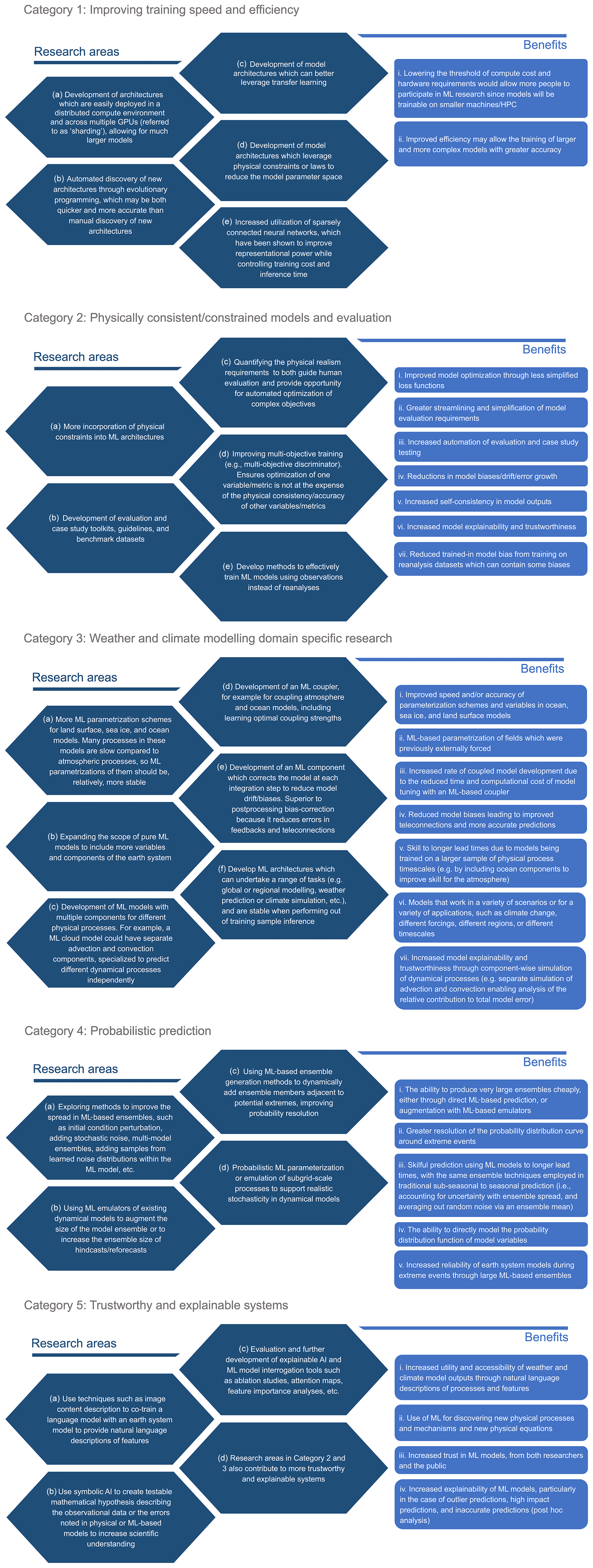
Figure 5Five categories for future ML research, including suggested research focusses for the community in each category and potential benefits which could be realized by research and development progress.
These categories are not mutually exclusive – indeed there is overlap between the research areas and benefits highlighted in each category (for example, some research foci in Categories 2 and 3 are also applicable to Category 5). The groupings are instead intended to help guide the focus of researchers and to provide a quick overview of the key topics where the community would most benefit from research progress.
Many of the research areas presented are complementary to each other; for example progress in making ML models more affordable to train (Category 1) will increase the utility of ML solutions to a wider community of researchers, and will likely accelerate the rate of progress in the other categories. Progress in the use of physically informed approaches (e.g. Category2, area a., or Category 3, area c.) could also lower the training cost of models by reducing the degree of redundancy in the model. On the other hand, approaches such as Category 3, area f., leading to an outcome such as benefit vi. would potentially reduce the demand for more cheaply trainable models since they could be readily turned to a variety of tasks, saving researchers the need to train their own model from scratch.
The research areas and ideas presented here are by no means a comprehensive list. Rather they are intended to be used as a source of inspiration, and the authors of this review are excited to see where the community chooses to focus their efforts in the coming years.
In this review we have presented a comprehensive survey of the literature on the use of ML in weather and climate modelling.
We have found that the ML models being most often explored include RFs and NNs, with a high prevalence of FCNNs and CNNs. We have also identified some recent innovations which have proven to be highly effective in the weather and climate modelling space, including DeepONets and variants thereof, Graph NNs, and PINNs.
This review has demonstrated that ML is being successfully applied to many aspects of weather and climate modelling. We have presented examples from the literature of its application in (1) the emulation and replacement of subgrid-scale parametrizations and super-parametrizations, (2) preconditioning and solving of resolved equations, (3) full-model replacement, and (4) a selection of other adjacent areas.
Nonetheless, there are still many research challenges to overcome, including
-
addressing the instabilities excited in physical models due to the inclusion of ML components;
-
increasing the ease of technical integration (in particular, Fortran compatibility);
-
memory and computational concerns;
-
representing a sufficient number of physical parameters and increasing physical and temporal resolution in ML-based weather and climate model implementations (which currently feature reduced fields and levels compared to physics-based numerical models);
-
moving from a focus on individual parts of the earth system (i.e. the atmosphere, the ocean, the land surface etc.) to tackling the challenges associated with coupled models (i.e. where models of individual components of the earth system are coupled together; increasingly, operational weather and climate models are coupled land–atmosphere–ocean–sea-ice models in order to more accurately represent the relevant timescales and processes in the earth system, and ML modelling efforts need to reflect this);
-
more thorough evaluation of the physical realism of ML-based predictions, at various length-scales, across parameters, and looking at the 3D structures;
-
exploring the use of generalized discriminators† to augment traditional loss functions in model training (to achieve a multivariate generalized objective function);
-
the need for more good quality training data; and
-
the practical challenges of integrating ML components or models into an operational setting.
This list, together with Sect. 11, provides a set of focus areas for future research efforts.
If the current trend in skill gains in full ML weather and climate models continues, it is possible they will eventually be considered viable alternatives to traditional numerical models. However in the meantime it is likely that ML components will replace an increasing number of physics-based model components, with models in the near-term future being hybrid ML–physical models. A likely future scenario is one where the best weather and climate models are a blend of ML and physics-based components, deriving skill from both data-driven and physical methodologies.
Some possible avenues through which increases in ML-based weather and climate model skill might be achieved is by operating at higher resolutions, by resolving more processes which are implicit in the training data, or by undertaking experiments on synthetic data to address the paucity of real-world data.
Another benefit of ML approaches to weather and climate modelling is the relative computational cheapness of ML alternatives to current physics-based modelling systems. This has the potential to open the door to experiments that would not be feasible otherwise. For example, experiments requiring a very large ensemble would be more feasible with a computationally cheap ML approach.
The literature reviewed here indicates that “out-of-the-box” ML approaches and architectures are not effective when used in a weather and climate modelling context. Rather, ML architectures must be adapted to satisfy conservation of energy, represent physically realistic predictions and processes, and maintain good model stability. At the same time, computational and memory tractability must be maintained.
Advances in the sophistication, complexity and efficiency of ML architectures are being heavily invested in for many use cases in other disciplines and in the private sector (e.g. condition–action pose estimation, text to video generation, stable diffusion, text to image, chatbots, facial recognition, and semantic image decomposition). In order to capture the full benefits of ML for the weather and climate modelling domain, academic and operational agencies will need to continue to support research in this space. This includes contributing to the research effort through foci such as those highlighted in Sect. 11 and in this section, as well as through addressing the particular challenges facing agencies interested in the operational and/or real-time deployment of ML-based models as the basis for services or the provision of advice (discussed in Sect. 9).
Interest and progress in the application of ML to weather and climate modelling has been present for close to 30 years and has begun to accelerate rapidly in the last few years. There is good reason to believe that ML as a tool will have transformational benefits and offer great potential for further application in weather and climate modelling.
This table includes all references from this review except for seminal ML papers that are on new ML methods (e.g. foundational ML papers), review papers, any paper cited that concerns a topic which is out of scope (e.g. nowcasting), and any other paper which does not present a new method directly applicable to weather and climate modelling.
Table A1Details of the papers cited in this review which contributed to the analysis presented in Figs. 1 and 3.
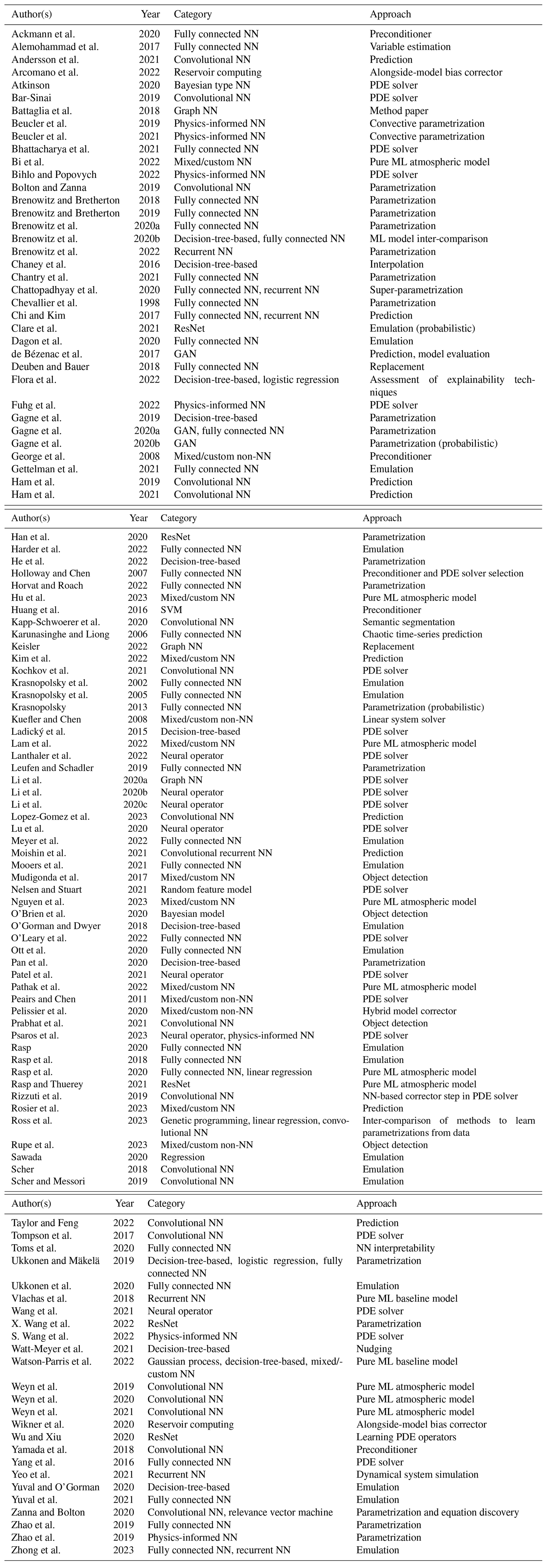
This glossary includes terms which the reader will come across frequently in machine learning literature for the weather and climate, as well as in machine learning literature generally. Most of these terms are used in this paper, while others require further reading.
Activation Function. The function which produces a neuron's outputs given its inputs. Commonly, this includes a learned bias term which is added to the data inputs before evaluation with a single function to produce the output value. Examples of the functions used include linear, sigmoid, and tanh.
Adversarial attack. The deliberate use of malicious data input in a real-world setting intended to cause a misclassification, underperformance, or unexpected behaviours. Examples include emails designed to avoid spam filters, or images that have been modified to avoid recognition. Adversarial example. A specialized input which results in a misclassification or underperformance of a predictive model. An example of this concept is an image which has had subtle noise added to it resulting in a copy of that image which is visually indistinguishable from the original but which nonetheless causes a misclassification. The term “adversarial” is used to refer to the way the example fools the model and is not necessarily intended to convey the sense of malicious intent, although the term is often applied in that fashion. Adversarial examples demonstrate that machine learning models may be more brittle than expected based on ordinary training data alone. To increase model robustness, adversarial examples may be generated and added to the training set. Data augmentation techniques such as flipping, warping, and adding noise (any many other techniques) are also used to generate additional training data to increase robustness and performance.
Attention mechanism. A mechanism to allow sequence prediction models to increase the importance of key terms within that sequence which may be non-local and modified in meaning according to the other terms of the sequence.
API (application programming interface). A set of programming functions, methods, or protocols by which to build and integrate applications. APIs may be “web” APIs or imported from software packages, in which case they are more often referred to as libraries.
Autoencoder. A neural network architecture which learns to produce a “code” for an input sequence from which the original data can be retrieved. The code is shorter than the original input sequence. Applications include data compression and denoising data.
Back propagation. A process of utilizing the errors from a prediction to update the weights and biases of a neural network.
Batch. See training batch.
Batch normalization. Data normalization which aligns the means and variances of input data to a model. For computational reasons, this is performed separately for each training batch.
Belief state. The current state of the world which is believed to be true according to a model. This is a common architecture in real-time applications whereby a belief state is updated according to an update function on the basis of new observations.
Channel. An additional dimension to data which is usually not a spatial dimension. Examples include the red, green, and blue intensity images which comprise a colour image. Another example could be to represent both temperature and wind speed as channels.
Classification. A model which attempts to diagnose or predict the category, label, class, or type that an example falls within.
Climatology. Refers to the usual past conditions for a location at a time of year. It is usually calculated by temporal mean across years of a dataset for a given time interval within those years (e.g. for a dataset of monthly mean values spanning all months of all years from 1990 to 2020, the monthly mean climatology would be obtained by averaging across all the Januaries from each year, all the Februaries, etc., to obtain an “average January”, an “average February”, etc.). Climatologies are often used in the same manner as persistence as a baseline prediction against which to measure a predictive model. For example, a model predicting a value for January could be compared to the climatological monthly mean value for January. This helps answer the question “is my model a better source of information than using the average past conditions from this time of year?”.
Connectome. The connections between nodes in a neural network. Examples include fully connected, partially connected, skip-layer connections, recurrent connections, and others. It is the “wiring diagram” for the network.
Convolutional neural network. A neural network architecture commonly applied to images which utilizes a convolutional (spatially connected) kernel applied in a sliding window fashion with a narrow receptive field to encourage the network to generalize from fine-scale structure to higher levels of abstraction.
Data augmentation. The practice of modifying input data in supervised learning to produce additional examples. This can make networks more robust to new inputs and address issues of brittleness to adversarial examples. An example of data augmentation is using rotated or reflected versions of the same image as independent training samples.
Data driven. A generalized term used to indicate a primary reliance or dependence on the collection or analysis of data. Used in contrast to process-driven or theory-driven approaches.
Decision tree. A tree-like, or flowchart-like, branching model representing a series of decisions and their possible consequences. Each internal node represents a “test” (i.e. decision threshold), and each leaf node represents a class label or collection of possible outcomes.
Deep NN. A neural network with many layers. Deeper, thinner networks have generally been more popular in recent times than wider, shallower ones, but this is not always the case (see e.g. Zagoruyko and Komodakis, 2016).
DeepONet. A neural network architecture relying on universal approximation theorem to train a neural network to represent a mathematical operation (the operator), such as a partial differential equation or dynamic system.
Discriminator model. A model which distinguishes or discriminates between synthetic data and real-world observations. Often used in conjunction with a generator. In this case, the overall goal is to produce a generator which is capable of fooling the discriminator, producing highly realistic images. This process is used in generative adversarial networks.
Dropout layer. A neural network layer which is only partially connected, often with a stochastic dropout chance. This has been shown experimentally to improve neural network robustness in many architectures by reducing overfitting.
Epoch. A single complete training pass through all available training data, e.g. learning from all samples or learning from all mini-batches, according to the training strategy. Multiple training epochs will typically be utilized, although alternative strategies do exist.
Feed-forward network. A neural network composed of distinct “layers”, where the outputs of one layer never feed back into earlier layers. This avoids the need for any iterative solver approaches and results in a very computationally efficient “forward pass”.
Generative adversarial network. A two-part neural network architecture comprising a generator and a discriminator, which are co-trained to produce realistic outputs that are hard to distinguish from real-world data. The discriminator replaces the traditional loss function.
Generator model. A model which produces a synthetic example of a particular class, such as a synthetic image or synthetic language. Examples include language or image generation. These are used as part of generative adversarial networks among other applications.
Global receptive field. Where every part of the input region can influence or stimulate a response in a model (e.g. a fully connected neural network).
GPU (graphical processing unit). A hardware device specialized for fast matrix operations, originally created to support computer graphics, particularly for games.
Gradient-boosted decision tree. Also referred to as extreme gradient boosting, a random forest architecture which combines gradient boosting with decision tree ensembles.
Gradient boosting. An approach to model training where each additional ensemble member attempts to predict the cumulative errors in previously trained members.
Graph neural network. A class of neural networks designed to process data, which is described by a graph, tree, or network data structure. See Scarselli et al. (2008), Kipf and Welling (2016), and Battaglia et al. (2018) for more information and examples.
Hidden layer. A layer which is intermediate between the input layer and the output layer of a network or tree structure. Hidden layers may be used to encode “hidden variables” which are latent to a problem but not able to be directly observed.
Hierarchical temporal aggregation. A mechanism of composing neural networks which are trained for different lead times to produce an optimal prediction at all time horizons.
Hierarchical temporal memory. Fundamentally different from hierarchical temporal aggregation, a complex deep learning architecture which uses time-adjacency pooling.
Hyperparameter. A parameter which is not derived via training. Examples include the learning rate and the model topology.
Hyperparameter search (or hyperparameter optimization). The process of determining optimal hyperparameters. This term may also be used to encompass the model selection problem. This process is automated in some cases.
Input layer. A layer which is composed of input nodes. Typically machine learning models will have one input layer at depth zero (i.e. with no preceding layers) and no input nodes at greater depths.
Input node. A node which represents an input or observed value.
K-fold cross-validation. A process of changing the validation and test data partitions during different iterations of training. This allows more of the training and validation data to be used while minimizing overfitting. Some definitions include test data in this process, but that is not ideal as the final test is no longer statistically independent.
Keras. A streamlined API for creating neural networks, integrated with TensorFlow, originally built on the Theano framework for general mathematical evaluation. PyTensor and Aesara are related packages.
Kernel trick. For datasets which are not linearly separable, first multiplying the data by a non-linear function in a higher dimension can result in a linearly separable higher-dimensional dataset with which a simpler method can be used to model the data.
Knowledge-based systems. A broad term from artificial intelligence meaning a system that uses reasoning and a knowledge base to support decision making. Knowledge is represented explicitly, and a reasoning or inference engine is used to arrive at new knowledge.
Layer. In tree or feed-forward network structures (e.g. decision trees and feed-forward neural networks), a layer refers to the set of nodes at the same depth within a network.
Leaf node (also known as the output node). A node which does not have any child nodes.
Long short-term memory network. A recurrent neural network architecture which processes sequences of tokens utilizing a “memory” component which can store information from tokens early in a sequence for use in the prediction of tokens much later in a sequence. Typical applications include language prediction and time-series prediction of many kinds.
Loss function (also known as target function, training function, objective function, penalty score, error function, heuristic function, and minimization function). A differentiable function which is well-behaved, such that smaller values represent better model performance and larger values represent worse performance. An example would be the root-mean-squared error in a prediction compared to the truth or target value.
Mini batch. A subset or “mini batch” of the training data, utilized for multiple reasons, including computational efficiency and to reduce overfitting. Aggregate error over a mini-batch is be learned rather than per-sample errors. This is the typical contemporary approach. See also training batch for in-depth discussion.
Neural network. A composition of “input nodes”, “connections”, “nodes”, “layers”, “output layers”, and “activation functions” which are capable of complex modelling tasks. It was originally designed to simulate human neural functioning and subsequently applied to a range of applications.
Node or vertex. A small data structure in a network, tree, or graph structure which is connected by edges. A node may represent a real-world value (such as a location), an abstract value (such as in a neural network), or a decision threshold (such as in a decision tree).
Normalization. A technique applied in many areas of mathematics, science, and statistics which is also very important to machine learning and neural networks. In a general sense, this refers to expressing values within a standard range. Very often, the range of expected values is mapped onto the range 0 to 1 to allow physical variables with different measurement units to be compared on equal scale. Such normalization may be linear or non-linear, according to a simple or more complex function, and either drawn from known physical limits or from the variation observed in the data themselves.
One-hot vector. A vector of 1s and 0s, in which only one bit is set to 1, typically produced during the first step in machine learning for language processing to create a word or feature embedding in a process called tokenization or encoding. The length of the vector is commonly equal to the number of categories or symbols.
Output layer. A layer which comprises the leaf nodes or output nodes of a tree or network.
Perceptron. A single-layer neural network architecture for supervised learning of binary classification, originally built as an electronic hardware device encoding weights with potentiometers and learning with motors. A multi-layer perceptron is the same thing as an ordinary neural network.
Persistence. Refers to the practice of treating some past observation or reanalysis (usually immediately prior to the starting point of the prediction period) as the future prediction and “persisting” this one state forward to every prediction lead time. The predictive model is then compared to this persistence prediction, essentially assessing the performance of the model against a steady state prediction. This, along with climatology, is often used as a baseline or bare minimum prediction to beat (i.e. a prediction better than persistence could be considered skilful vs. persistence). This answers the question “is my model a better source of information than using what happened just before now?”.
Physically informed machine learning (also known as physics-informed machine learning). Machine learning is considered physically informed when some aspect of physics is included in any way. Examples include adding a physical component to the loss function (e.g. to enforce conservation of physical properties) or using an activation function with physically realistic properties.
Predictive step, forward pass, evaluation. The process of calculating a model prediction from a set of input conditions. It is distinct from the training phase or back-propagation step.
PyTorch. A widely adopted framework for neural networks in Python.
Random forest. An architecture based on decision tree ensembles where each decision tree is initialized semi-randomly and an average of all models is used for prediction. This is typically more accurate than a single decision tree but less accurate than a gradient-boosted decision tree and so is now less used. The term random forest is still commonly used when in fact the implementation is a gradient-boosted decision tree.
Receptive field. The size or extent of a region in the input which can influence or stimulate a response in a model, e.g. the size of a convolutional kernel and the size of a sliding window.
Rectified linear unit (ReLU). An activation function commonly used in NNs. Defined as max(0, X), this function is used as it is computationally cheap and avoids problems of vanishing gradients.
Recurrent network. A neural network which does pass the output from nodes of the network back into the input of others. Infinite recurrence is avoided by setting a specific number of iterations for the recurrence. These are often depicted in diagrams as separate layers, but the implementation is through internal recurrent connections.
Regression. A model which attempts to diagnose or predict an exact value by statistically relating example input values to desired values.
Relevance vector machine. A sparse Bayesian model utilizing the kernel trick in similar fashion to a support vector machine.
Representation error. Error which is introduced due to the inexactness of representing the real world in the model belief state. Examples may include topography smoothing, point-to-grid translations, model grid distortions near the poles, or the exclusion of physical characteristics which are not primary to the model.
Residual neural network (ResNet). A very influential and innovative convolutional NN architecture which uses a similar concept to gradient boosting. Each layer of the deep network is taken to predict the residual error from the previous layers, with skip connections from earlier layers allowing the training to occur without the issue of vanishing gradients.
Sample. A single training example (e.g. a row of data).
Scale invariance. A feature of a system, problem, or model, which means the results and behaviour are the same at any scale (e.g. the behaviour does not change if the inputs are multiplied by a common factor).
Scikit-learn. A popular Python library for machine learning which extends the SciPy framework.
Sharding. Refers to dividing the training of a neural network across multiple GPUs or nodes. This can be done using data sharding, whereby each GPU or node trains on a subset of the data to allow training parallelism or model sharding where a single model is partitioned across multiple GPUs to allow a larger neural network than could be allocated in memory on a single GPU. One example could be assigning a small number of neural network layers to each GPU, which could then work in sequence to operate on a very large network.
(Stochastic) gradient descent. An algorithm by which a neural network is trained using increasingly fine-scale adjustments to optimize the accuracy of network prediction, utilized to find the local minimum of a differentiable function.
Supervised learning. Machine learning is considered “supervised” when the data are labelled according to a category or target value. Classification data have an explicit labelled category. Regression data have an explicit value which is being predicted for.
Support vector machine. A classification model based on finding a hyperplane to separate data utilizing the kernel trick.
Tensor. Can be considered as a dense, multi-dimensional array or matrix.
TensorFlow. A widely adopted framework for neural networks in Python.
Test/train/validate split. Available data are split into three portions. The training data are evaluated and used to update model weights. Validation data are evaluated during training and may be used for hyper-parameter search or to guide the researcher. Test data are independent (typically well-curated) data used for gold standard evaluation. In reality, validation data are sometimes used as test data, but this is not good practice. There are many considerations for test/train/validate splitting, such as statistical independence, representation of all classes, and bias. It is important to consider what the model is generalizing “from” and “to” and ensuring appropriate examples are present in the training data and appropriate examples are reserved for validation and test.
Token. Tokenization the process of mapping a symbolic or categorical sequence to a numerical representation which is suited to a sequence-based machine learning model. Commonly, a vector representation will be utilized for the token form. In language processing, either characters or words may be represented as tokens depending on the approach.
Top hat function. A filter or function which has a rectangular shape resembling the cross-section of a top hat. One of the simplest functions used for convolutional operations, it can be defined as one constant value in a given bounded range, and another smaller constant value outside that range.
TPU (tensor processing unit.) A hardware device specialized for artificial intelligence and machine learning applications, in particular neural network operations.
Training batch (or simply batch). Multiple definitions apply and the use the term has evolved over time, originally used in the context of learning from offline or saved historical data as opposed to online or real-time novel data. In this definition, the training batch is the saved data and refers to the whole training set. For example, a robot exploring a new environment in real-time must use an online learning technique and can not utilize batch training to map the unseen terrain. In more recent use, particularly in the areas of neural network learning, the offline saved data may be split into one or more batches (subsets). If one batch (the batch is the entire training set) is used, the aggregate errors for the entire training set are used to update the model weights and biases, and the learning algorithm is called batch gradient descent. If each example is presented individually, this is called online training (even when historical saved data are being used), the weights and biases are updated for from each individual example, and the algorithm used is stochastic gradient descent. If the data are divided into multiple batches, this is often referred to equivalently as mini batches. The weights and biases are aggregated over each mini batch. This is the most common contemporary approach, as it reduces overfitting and is a good balance of training accuracy, avoiding local minima, and computational efficiency.
Transfer learning. The process of training a model first on a related problem and then conducting further training on a more specific problem. Examples could be training a model first in one geographical region and then in another or training first at a low resolution and then subsequently at a high resolution. This is frequently done to reduce training computation cost for similar problems by re-using the trained weights from a well-performing source model or to overcome a problem of limited data availability by using multiple data sources.
Transformer network. A token-sequence architecture which is capable of handling long-range dependencies. Initially applied to language processing, it has found effective application in image processing as an alternative to convolutional architectures.
Translation invariance. A feature of a system, problem, or model, which means the results and behaviour are the same after any spatial translation (i.e. the behaviour does not change if the inputs are shifted spatially to a new location).
U-Net. A type of convolutional neural network developed for biomedical image segmentation which has found broad application. In the contracting part of the network spatial information is reduced, while feature information is increased. In the expanding part of the network, feature information is used to inform us of high-resolution segmentation. The name derives from the diagrammatic shape of the network forming a “U”.
Unsupervised learning. Machine learning is considered “unsupervised” when data are unlabelled. Examples include clustering, association, and dimensionality reduction.
Vanishing gradient. At the extremes, non-linear functions used to calculate gradients can result in gradient values which are effectively zero. These small or zero values, once present in the weights and biases of a neural network, can entirely suppress information, which would in fact be useful, and result in a local minima from which training cannot recover. This is particularly relevant to long token series when long-distance connections are relevant. A variety of techniques including alternative activation functions, training weight decay, skip connections, and attention mechanisms may each or all be utilized to ameliorate this issue.
Weights and biases. The parameter values for each neuron which represent the weighting factors to apply to the input values, as well as an overall bias value for the node.
XGBoost. A popular Python library for gradient-boosted decision trees.
No code was used in the preparation of this review. No data were processed in the preparation of this review except for the list of ML model types by cited paper, which is provided in Appendix A.
COdBD researched and wrote Sects. 3, 4, 5, 6, and 7 and provided review of Sects. 8 and 10 and Appendix B. TL researched and wrote Sects. 8 and 10 and Appendix B and provided review of Sects. 3, 4, 5, 6, and 7. COdBD and TL researched and co-wrote Sects. 1, 2, 9, 11, and 12 and Appendix A.
The contact author has declared that neither of the authors has any competing interests.
Publisher's note: Copernicus Publications remains neutral with regard to jurisdictional claims made in the text, published maps, institutional affiliations, or any other geographical representation in this paper. While Copernicus Publications makes every effort to include appropriate place names, the final responsibility lies with the authors.
The authors would like to thank Bethan White, Harrison Cook, Tom Dunstan, and Karina Williams for their very helpful reviews of early versions of this paper. We also would like to wholeheartedly thank the referees for their extremely helpful, positive, and well-considered feedback and suggestions. Their input has greatly improved this review. Finally, we would like to acknowledge and thank the people who contacted us with comments, suggestions, and advice on the preprint versions of this review. All of the input was valuable and greatly appreciated.
This paper was edited by Paul Ullrich and David Ham, and reviewed by two anonymous referees.
Ackmann, J., Düben, P. D., Palmer, T. N., and Smolarkiewicz, P. K.: Machine-learned preconditioners for linear solvers in geophysical fluid flows, arXiv [preprint], https://doi.org/10.48550/arXiv.2010.02866, 6 October 2020.
Adams, S. V., Ford, R. W., Hambley, M., Hobson, J. M., Kavčič, I., Maynard, C. M., Melvin, T., Müller, E. H., Mullerworth, S., Porter, A. R. Rezny, M., Shipway, B. J., and Wong, R.: LFRic: Meeting the challenges of scalability and performance portability in Weather and Climate models, J. Parallel. Distr. Com., 132, 383–396, https://doi.org/10.1016/j.jpdc.2019.02.007, 2019.
Alemohammad, S. H., Fang, B., Konings, A. G., Aires, F., Green, J. K., Kolassa, J., Miralles, D., Prigent, C., and Gentine, P.: Water, Energy, and Carbon with Artificial Neural Networks (WECANN): a statistically based estimate of global surface turbulent fluxes and gross primary productivity using solar-induced fluorescence, Biogeosciences, 14, 4101–4124, https://doi.org/10.5194/bg-14-4101-2017, 2017.
: Andersson, T. R., Hosking, J. S., Pérez-Ortiz, M., Paige, B., Elliott, A., Russell, C., Law, S., Jones, D. C., Wilkinson, J., Phillips, T., Byrne, J., Tietsche, S., Sarojini, B. B., Blanchard-Wrigglesworth, E., Aksenov, Y., Downie, R., and Shuckburgh, E.: Seasonal Arctic sea ice forecasting with probabilistic deep learning, Nat. Commun., 12, 5124, https://doi.org/10.1038/s41467-021-25257-4. 2021.
Arcomano, T., Szunyogh, I., Wikner, A., Pathak, J., Hunt, B. R., and Ott, E.: A Hybrid Approach to Atmospheric Modeling That Combines Machine Learning With a Physics-Based Numerical Model, J. Adv. Model. Earth Sy., 14, e2021MS002712, https://doi.org/10.1029/2021MS002712, 2022.
Atkinson, S.: Bayesian hidden physics models: Uncertainty quantification for discovery of nonlinear partial differential operators from data, arXiv [preprint], https://doi.org/10.48550/arXiv.2006.04228. 7 June 2020.
Bar-Sinai, Y., Hoyer, S., Hickey, J., and Brenner, M. P.: Learning data-driven discretizations for partial differential equations, P. Natl. Acad. Sci. USA, 116, 15344–15349, https://doi.org/10.1073/pnas.1814058116. 2019.
Battaglia, P. W., Hamrick, J. B., Bapst, V., Sanchez-Gonzalez, A., Zambaldi, V., Malinowski, M., Tacchetti, A., Raposo, D., Santoro, A., Faulkner, R. and Gulcehre, C., Song, F., Ballard, A., Gilmer, J., Dahl, G., Vaswani, A., Allen, K., Nash, C., Langston, V., Dyer, C., Heess, N., Wierstra, D., Kohli, P., Botvinick, M., Vinyals, O., Li, Y., and Pascanu R.: Relational inductive biases, deep learning, and graph networks, arXiv [preprint], https://doi.org/10.48550/arXiv.1806.01261, 4 June 2018.
Beucler, T., Rasp, S., Pritchard, M., and Gentine, P.: Achieving conservation of energy in neural network emulators for climate modeling, arXiv [preprint], https://doi.org/10.48550/arXiv.1906.06622, 15 June 2019.
Beucler, T., Pritchard, M., Rasp, S., Ott, J., Baldi, P., and Gentine, P.: Enforcing analytic constraints in neural networks emulating physical systems, Phys. Rev. Lett., 126, 098302, https://doi.org/10.1103/PhysRevLett.126.098302. 2021.
Bhattacharya, K., Hosseini, B., Kovachki, N. B., and Stuart, A. M.: Model reduction and neural networks for parametric PDEs, arXiv [preprint], https://doi.org/10.48550/arXiv.2005.03180, 7 May 2020.
Bi, K., Xie, L., Zhang, H., Chen, X., Gu, X., and Tian, Q.: Pangu-Weather: A 3D High-Resolution Model for Fast and Accurate Global Weather Forecast, arXiv [preprint], https://doi.org/10.48550/arXiv.2211.02556, 3 November 2022.
Bihlo, A. and Popovych, R. O.: Physics-informed neural networks for the shallow-water equations on the sphere, J. Comput. Phys., 456, 111024, https://doi.org/10.1016/j.jcp.2022.111024. 2022.
Bolton, T. and Zanna, L.: Applications of deep learning to ocean data inference and subgrid parameterization, J. Adv. Model. Earth Sy., 11, 376–399, https://doi.org/10.1029/2018MS001472, 2019.
Breiman, L.: Random forests, Mach. Learn., 45, 5–32, 2001.
Brenowitz, N. D. and Bretherton, C. S.: Prognostic validation of a neural network unified physics parameterization, Geophys. Res. Lett., 45, 6289–6298, https://doi.org/10.1029/2018GL078510, 2018.
Brenowitz, N. D. and Bretherton, C. S.: Spatially extended tests of a neural network parametrization trained by coarse-graining, J. Adv. Model. Earth Sy., 11, 2728–2744, https://doi.org/10.1029/2019MS001711, 2019.
Brenowitz, N. D., Beucler, T., Pritchard, M., and Bretherton, C. S.: Interpreting and stabilizing machine-learning parametrizations of convection, J. Atmos. Sci., 77, 4357–4375, https://doi.org/10.1175/JAS-D-20-0082.1, 2020a.
Brenowitz, N. D., Henn, B., McGibbon, J., Clark, S. K., Kwa, A., Perkins, W. A., Watt-Meyer, O., and Bretherton, C. S.: Machine learning climate model dynamics: Offline versus online performance, arXiv [preprint], https://doi.org/10.48550/arXiv.2011.03081, 5 November 2020b.
Brenowitz, N. D., Perkins, W. A., Nugent, J. M., Watt-Meyer, O., Clark, S. K., Kwa, A., Henn, B., McGibbon, J., and Bretherton, C. S.: Emulating Fast Processes in Climate Models., arXiv [preprint], https://doi.org/10.48550/arXiv.2211.10774, 19 November 2022.
Carranza-García, M., García-Gutiérrez, J., and Riquelme, J. C.: A framework for evaluating land use and land cover classification using convolutional neural networks, Remote Sens.-Basel, 11, 274, https://doi.org/10.3390/rs11030274, 2019.
Chaney, N. W., Herman, J. D., Ek, M. B., and Wood, E. F.: Deriving global parameter estimates for the Noah land surface model using FLUXNET and machine learning, J. Geophys. Res.-Atmos., 121, 13–218, https://doi.org/10.1002/2016JD024821, 2016.
Chantry, M., Christensen, H., Dueben, P., and Palmer, T.: Opportunities and challenges for machine learning in weather and climate modelling: hard, medium and soft AI, Philos. T. Roy. Soc. A, 379, 20200083, https://doi.org/10.1098/rsta.2020.0083, 2021a.
Chantry, M., Hatfield, S., Dueben, P., Polichtchouk, I., and Palmer, T.: Machine learning emulation of gravity wave drag in numerical weather forecasting, J. Adv. Model. Earth Sy., 13, e2021MS002477, https://doi.org/10.1029/2021MS002477, 2021b.
Chase, R. J., Harrison, D. R., Burke, A., Lackmann, G. M., and McGovern, A.: A Machine Learning Tutorial for Operational Meteorology, Part I: Traditional Machine Learning, arXiv [preprint], https://doi.org/10.48550/arXiv.2204.07492, 2022a.
Chase, R. J., Harrison, D. R., Lackmann, G., and McGovern, A.: A Machine Learning Tutorial for Operational Meteorology, Part II: Neural Networks and Deep Learning, arXiv [preprint], https://doi.org/10.48550/arXiv.2211.00147, 2022b.
Chattopadhyay, A., Subel, A., and Hassanzadeh, P.: Data-driven super-parameterization using deep learning: Experimentation with multiscale lorenz 96 systems and transfer learning, J. Adv. Model. Earth Sy., 12, e2020MS002084, https://doi.org/10.1029/2020MS002084, 2020.
Chevallier, F., Chéruy, F., Scott, N. A., and Chédin, A.: A neural network approach for a fast and accurate computation of a longwave radiative budget, J. Appl. Meteorol., 37, 1385–1397, https://doi.org/10.1175/1520-0450(1998)037%3C1385:ANNAFA%3E2.0.CO;2, 1998.
Chi, J. and Kim, H. C. Prediction of arctic sea ice concentration using a fully data driven deep neural network, Remote Sens.-Basel, 9, 1305, https://doi.org/10.3390/rs9121305, 2017.
Clare, M. C., Jamil, O., and Morcrette, C. J.: Combining distribution-based neural networks to predict weather forecast probabilities, Q. J. Roy. Meteor. Soc., 147, 4337–4357, https://doi.org/10.1002/qj.4180, 2021.
Cuomo, S., Di Cola, V. S., Giampaolo, F., Rozza, G., Raissi, M., and Piccialli, F.: Scientific Machine Learning through Physics-Informed Neural Networks: Where we are and What's next, arXiv [preprint], https://doi.org/10.48550/arXiv.2201.05624, 14 January 2022.
Dagon, K., Sanderson, B. M., Fisher, R. A., and Lawrence, D. M.: A machine learning approach to emulation and biophysical parameter estimation with the Community Land Model, version 5, Adv. Stat. Clim. Meteorol. Oceanogr., 6, 223–244, https://doi.org/10.5194/ascmo-6-223-2020, 2020.
De Bézenac, E., Pajot, A., and Gallinari, P.: Towards a hybrid approach to physical process modeling, Technical report, https://dl4physicalsciences.github.io/files/nips_dlps_2017_9.pdf (last access: 3 November 2023), 2017.
de Witt, C. S., Tong, C., Zantedeschi, V., De Martini, D., Kalaitzis, F., Chantry, M., Watson-Parris, D., and Bilinski, P.: RainBench: towards global precipitation forecasting from satellite imagery, arXiv [preprint], https://doi.org/10.48550/arXiv.2012.09670, 17 December 2020.
Deng, J., Dong, W., Socher, R., Li, L. J., Li, K., and Fei-Fei, L.: Imagenet: A large-scale hierarchical image database, IEEE Conference on Computer Vision and Pattern Recognition, Miami, FL, USA, 248–255, https://doi.org/10.1109/CVPR.2009.5206848, 2009.
Digra, M., Dhir, R., and Sharma, N.: Land use land cover classification of remote sensing images based on the deep learning approaches: a statistical analysis and review, Arab. J. Geosci., 15, 1003, https://doi.org/10.1007/s12517-022-10246-8, 2022.
Dosovitskiy, A., Beyer, L., Kolesnikov, A., Weissenborn, D., Zhai, X., Unterthiner, T., Dehghani, M., Minderer, M., Heigold, G., Gelly, S. Uszkoreit, J., and Houlsby, N.: An image is worth 16x16 words: Transformers for image recognition at scale, arXiv [preprint], https://doi.org/10.48550/arXiv.2010.11929, 22 October 2020.
Dueben, P. D. and Bauer, P.: Challenges and design choices for global weather and climate models based on machine learning, Geosci. Model Dev., 11, 3999–4009, https://doi.org/10.5194/gmd-11-3999-2018, 2018.
Dueben, P. D., Schultz, M. G., Chantry, M., Gagne, D. J., Hall, D. M., and McGovern, A.: Challenges and Benchmark Datasets for Machine Learning in the Atmospheric Sciences: Definition, Status, and Outlook, Artificial Intelligence for the Earth Systems, 1, e210002, https://doi.org/10.1175/AIES-D-21-0002.1, 2022.
ECMWF: Ifs documentation (cy45r1), https://www.ecmwf.int/en/publications/ifs-documentation (last access: 7 February 2023), 2018.
Eyring, V., Bony, S., Meehl, G. A., Senior, C. A., Stevens, B., Stouffer, R. J., and Taylor, K. E.: Overview of the Coupled Model Intercomparison Project Phase 6 (CMIP6) experimental design and organization, Geosci. Model Dev., 9, 1937–1958, https://doi.org/10.5194/gmd-9-1937-2016, 2016.
Flora, M., Potvin, C., McGovern, A., and Handler, S.: Comparing Explanation Methods for Traditional Machine Learning Models Part 2: Quantifying Model Explainability Faithfulness and Improvements with Dimensionality Reduction, arXiv [preprint], https://doi.org/10.48550/arXiv.2211.10378, 18 November 2022.
Friedman, J. H.: Greedy function approximation: a gradient boosting machine, Ann. Stat., 29 1189–1232, https://doi.org/10.1214/aos/1013203451, 2001.
Fuhg, J. N., Kalogeris, I., Fau, A., and Bouklas, N.: Interval and fuzzy physics-informed neural networks for uncertain fields, Probabilist. Eng. Mech., 68, 103240, https://doi.org/10.1016/j.probengmech.2022.103240, 2022.
Gagne, D. J., McCandless, T., Kosovic, B., DeCastro, A., Loft, R., Haupt, S. E., and Yang, B.: Machine learning parameterization of the surface layer: bridging the observation-modeling gap, in: AGU Fall Meeting Abstracts, Vol. 2019, IN44A-04, https://ui.adsabs.harvard.edu/abs/2019AGUFMIN44A..04G/abstract (last access: 3 November 2023), 2019.
Gagne, D. J., Chen, C. C., and Gettelman, A.: Emulation of bin Microphysical Processes with machine learning, in: 100th American Meteorological Society Annual Meeting, AMS, https://ams.confex.com/ams/2020Annual/webprogram/Paper368156.html (last access: 3 November 2023), 2020a.
Gagne, D. J., Christensen, H. M., Subramanian, A. C., and Monahan, A. H.: Machine learning for stochastic parameterization: Generative adversarial networks in the Lorenz'96 model, J. Adv. Model. Earth Sy., 12, e2019MS001896, https://doi.org/10.1029/2019MS001896, 2020b.
Garg, S., Rasp, S., and Thuerey, N.: WeatherBench Probability: A benchmark dataset for probabilistic medium-range weather forecasting along with deep learning baseline models, arXiv [preprint], https://doi.org/10.48550/arXiv.2205.00865, 2 May 2022.
George, T., Gupta, A., and Sarin, V.: A recommendation system for preconditioned iterative solvers, Eighth IEEE International Conference on Data Mining, Pisa, Italy, 803–808, https://doi.org/10.1109/ICDM.2008.105, 2008.
Gettelman, A., Gagne, D. J., Chen, C. C., Christensen, M. W., Lebo, Z. J., Morrison, H., and Gantos, G.: Machine learning the warm rain process, J. Adv. Model. Earth Sy., 13, e2020MS002268, https://doi.org/10.1029/2020MS002268, 2021.
Goodfellow, I., Yoshua B., and Aaron C.: Deep learning, MIT press, ISBN 9780262035613, 2016.
Goodfellow, I., Pouget-Abadie, J., Mirza, M., Xu, B., Warde-Farley, D., Ozair, S., Courville, A., and Bengio, Y.: Generative adversarial networks, Commun. Acm., 63, 139–144, https://doi.org/10.1145/3422622, 2020.
Grigo, C. and Koutsourelakis, P. S.: A physics-aware, probabilistic machine learning framework for coarse-graining high-dimensional systems in the Small Data regime, J. Comput. Phys., 397, 108842, https://doi.org/10.1016/j.jcp.2019.05.053, 2019.
Gurvan, M., Bourdallé-Badie, R., Chanut, J., Clementi, E., Coward, A., Ethé, C., Iovino, D., Lea, D., Lévy, C., Lovato, T., Martin, N., Masson, S., Mocavero, S., Rousset, C., Storkey, D., Vancoppenolle, M., Müeller, S., Nurser, G., Bell, M., and Samson, G.: NEMO ocean engine, Institut Pierre-Simon Laplace (IPSL), Zenodo, https://doi.org/10.5281/zenodo.1464816, 2019.
Ham, Y. G., Kim, J. H., and Luo, J. J.: Deep learning for multi-year ENSO forecasts, Nature, 573, 568–572, https://doi.org/10.1038/s41586-019-1559-7, 2019.
Ham, Y. G., Kim, J. H., Kim, E. S., and On, K. W.: Unified deep learning model for El Niño/Southern Oscillation forecasts by incorporating seasonality in climate data, Sci. Bull., 66, 1358–1366, https://doi.org/10.1016/j.scib.2021.03.009, 2021.
Han, Y., Zhang, G. J., Huang, X., and Wang, Y.: A moist physics parameterization based on deep learning, J. Adv. Model. Earth Sy., 12, e2020MS002076, https://doi.org/10.1029/2020MS002076, 2020.
Harder, P., Watson-Parris, D., Stier, P., Strassel, D., Gauger, N. R., and Keuper, J.: Physics-informed learning of aerosol microphysics, Environ. Data Sci., 1, e20, https://doi.org/10.1017/eds.2022.22, 2022.
Harris, L., Chen, X., Putman, W., Zhou, L., and Chen, J. H.: A scientific description of the GFDL finite-volume cubed-sphere dynamical core, NOAA technical memorandum OAR GFDL, https://doi.org/10.25923/6nhs-5897, 2021.
Hastie, T., Tibshirani, R., Friedman, J. H., and Friedman, J. H.: The elements of statistical learning: data mining, inference, and prediction, New York Springer, 2, 758 pp., https://doi.org/10.1007/978-0-387-21606-5, 2009.
He, K., Zhang, X., Ren, S., and Sun, J.: Deep residual learning for image recognition, Proc. CVPR IEEE, 770–778, https://doi.org/10.48550/arXiv.1512.03385, 2016.
He, X., Liu, S., Xu, T., Yu, K., Gentine, P., Zhang, Z., Xu, Z., Jiao, D., and Wu, D.: Improving predictions of evapotranspiration by integrating multi-source observations and land surface model, Agr. Water Manage., 272, 107827, https://doi.org/10.1016/j.agwat.2022.107827, 2022.
Hewamalage, H., Ackermann, K., and Bergmeir, C.: Forecast Evaluation for Data Scientists: Common Pitfalls and Best Practices, arXiv [preprint], https://doi.org/10.48550/arXiv.2203.10716, 21 March 2022.
Hochreiter, S. and Schmidhuber, J.: LSTM can solve hard long time lag problems, Adv. Neur. In., 9, https://papers.nips.cc/paper_files/paper/1996/hash/a4d2f0d23dcc84ce983ff9157f8b7f88-Abstract.html (last access: 3 November 2023), 1996.
Holloway, A. and Chen, T. Y.: Neural networks for predicting the behavior of preconditioned iterative solvers, in: International Conference on Computational Science,Springer, Berlin, Heidelberg, 302–309, https://doi.org/10.1007/978-3-540-72584-8_39, 2007.
Hornik, K., Stinchcombe, M., and White, H.: Multilayer feedforward networks are universal approximators, Neural Networks, 2, 359–366, https://doi.org/10.1016/0893-6080(89)90020-8, 1989.
Horvat, C. and Roach, L. A.: WIFF1.0: a hybrid machine-learning-based parameterization of wave-induced sea ice floe fracture, Geosci. Model Dev., 15, 803–814, https://doi.org/10.5194/gmd-15-803-2022, 2022.
Hsieh, W. W.: Introduction to Environmental Data Science, Cambridge University Press, https://doi.org/10.1017/9781107588493, 2023.
Hu, Y., Chen, L., Wang, Z., and Li, H.: SwinVRNN: A Data-Driven Ensemble Forecasting Model via Learned Distribution Perturbation, J. Adv. Model. Earth Sy., 15, e2022MS003211, https://doi.org/10.1029/2022MS003211, 2023.
Huang, Z., England, M., Davenport, J. H., and Paulson, L. C.: Using machine learning to decide when to precondition cylindrical algebraic decomposition with Groebner bases, 18th International Symposium on Symbolic and Numeric Algorithms for Scientific Computing (SYNASC), Timisoara, Romania, 45–52, https://doi.org/10.1109/SYNASC.2016.020, 2016.
Johnson, S. J., Stockdale, T. N., Ferranti, L., Balmaseda, M. A., Molteni, F., Magnusson, L., Tietsche, S., Decremer, D., Weisheimer, A., Balsamo, G., Keeley, S. P. E., Mogensen, K., Zuo, H., and Monge-Sanz, B. M.: SEAS5: the new ECMWF seasonal forecast system, Geosci. Model Dev., 12, 1087–1117, https://doi.org/10.5194/gmd-12-1087-2019, 2019.
Kapp-Schwoerer, L., Graubner, A., Kim, S., and Kashinath, K.: Spatio-temporal segmentation and tracking of weather patterns with light-weight Neural Networks, https://ai4earthscience.github.io/neurips-2020-workshop/papers/ai4earth_neurips_2020_55.pdf (last access: 3 November 2023), 2020.
Karpatne, A., Atluri, G., Faghmous, J. H., Steinbach, M., Banerjee, A., Ganguly, A., Shekhar, S., Samatova, N., and Kumar, V.: Theory-guided data science: A new paradigm for scientific discovery from data, IEEE T. Knowl. Data En., 29, 2318–2331, https://doi.org/10.1109/TKDE.2017.2720168, 2017.
Karunasinghe, D. S. and Liong, S. Y.: Chaotic time series prediction with a global model: Artificial neural network, J. Hydrol., 323, 92–105, https://doi.org/10.1016/j.jhydrol.2005.07.048, 2006.
Kashinath, K., Mustafa, M., Albert, A., Wu, J. L., Jiang, C., Esmaeilzadeh, S., Azizzadenesheli, K., Wang, R., Chattopadhyay, A., Singh, A., Manepalli, A., Chirila, D., Yu, R., Walters, R., White, B., Xiao, H., Tchelepi, H. A., Marcus, P., Anandkumar, A., Hassanzadeh, P., and Prabhat, N.: Physics-informed machine learning: case studies for weather and climate modelling, Philos. T. Roy. Soc. A, 379, 20200093, https://doi.org/10.1098/rsta.2020.0093, 2021.
Keisler, R.: Forecasting Global Weather with Graph Neural Networks, arXiv [preprint], https://doi.org/10.48550/arXiv.2202.07575, 15 February 2022.
Kelotra, A. and Pandey, P.: Stock market prediction using optimized deep-convlstm model, Big Data, 8, 5–24, https://doi.org/10.48550/arXiv.2202.07575, 2022.
Kim, J., Kwon, M., Kim, S. D., Kug, J. S., Ryu, J. G., and Kim, J.: Spatiotemporal neural network with attention mechanism for El Niño forecasts, Sci. Rep.-UK, 12, 1–15, https://doi.org/10.1038/s41598-022-10839-z, 2022.
Kipf, T. N. and Welling, M.: Semi-supervised classification with graph convolutional networks, arXiv [preprint], https://doi.org/10.48550/arXiv.1609.02907, 9 September 2016.
Kochkov, D., Smith, J. A., Alieva, A., Wang, Q., Brenner, M. P., and Hoyer, S.: Machine learning–accelerated computational fluid dynamics, P. Natl. Acad. Sci. USA, 118, e2101784118, https://doi.org/10.1073/pnas.2101784118, 2021.
Krasnopolsky, V. M., Chalikov, D. V., and Tolman, H. L.: A neural network technique to improve computational efficiency of numerical oceanic models, Ocean Model., 4, 363–383, https://doi.org/10.1016/S1463-5003(02)00010-0, 2002.
Krasnopolsky, V. M., Fox-Rabinovitz, M. S., and Chalikov, D. V.: New approach to calculation of atmospheric model physics: Accurate and fast neural network emulation of longwave radiation in a climate model, Mon. Weather Rev., 133, 1370–1383, https://doi.org/10.1175/MWR2923.1, 2005.
Krasnopolsky, V. M., Fox-Rabinovitz, M. S., and Belochitski, A. A.: Using ensemble of neural networks to learn stochastic convection parameterizations for climate and numerical weather prediction models from data simulated by a cloud resolving model, Advances in Artificial Neural Systems, 2013, p. 5, https://doi.org/10.1155/2013/485913, 2013.
Kuefler, E. and Chen, T. Y.: On using reinforcement learning to solve sparse linear systems, in: International Conference on Computational Science, Springer, Berlin, Heidelberg, 955–964, https://doi.org/10.1007/978-3-540-69384-0_100, 2008.
Ladický, L. U., Jeong, S., Solenthaler, B., Pollefeys, M., and Gross, M.: Data-driven fluid simulations using regression forests, ACM T. Graphic., 34, 1–9, https://doi.org/10.1145/2816795.2818129, 2015.
Lam, R., Sanchez-Gonzalez, A., Willson, M., Wirnsberger, P., Fortunato, M., Pritzel, A., Ravuri, S., Ewalds, T., Alet, F., Eaton-Rosen, Z. Hu, W., Merose, A., Hoyer, S., Holland, G., Vinyals, O., Stott, J., Pritzel, A., Mohamed, S., and Battaglia, P.: GraphCast: Learning skillful medium-range global weather forecasting, arXiv [preprint], https://doi.org/10.48550/arXiv.2212.12794, 24 December 2022.
Lanthaler, S., Mishra, S., and Karniadakis, G. E.: Error estimates for deeponets: A deep learning framework in infinite dimensions, T. Math. Appl., 6, tnac001, https://doi.org/10.1093/imatrm/tnac001, 2022.
LeCun, Y., Bottou, L., Bengio, Y., and Haffner, P.: Gradient-based learning applied to document recognition, P. IEEE, 86, 2278–2324, https://doi.org/10.1109/5.726791, 1998.
Leufen, L. H. and Schädler, G.: Calculating the turbulent fluxes in the atmospheric surface layer with neural networks, Geosci. Model Dev., 12, 2033–2047, https://doi.org/10.5194/gmd-12-2033-2019, 2019.
Li, Z., Kovachki, N., Azizzadenesheli, K., Liu, B., Stuart, A., Bhattacharya, K., and Anandkumar, A.: Multipole graph neural operator for parametric partial differential equations, Adv. Neur. In., 33, 6755–6766, 2020a.
Li, Z., Kovachki, N., Azizzadenesheli, K., Liu, B., Bhattacharya, K., Stuart, A., and Anandkumar, A.: Neural operator: Graph kernel network for partial differential equations, arXiv [preprint], https://doi.org/10.48550/arXiv.2003.03485, 7 March 2020b.
Li, Z., Kovachki, N., Azizzadenesheli, K., Liu, B., Bhattacharya, K., Stuart, A., and Anandkumar, A.: Fourier neural operator for parametric partial differential equations, arXiv [preprint], https://doi.org/10.48550/arXiv.2010.08895, 18 October 2020c.
Lopez-Gomez, I., McGovern, A., Agrawal, S., and Hickey, J.: Global extreme heat forecasting using neural weather models, Artificial Intelligence for the Earth Systems, 2, e220035, https://doi.org/10.1175/AIES-D-22-0035.1, 2023.
Lorenz, E. N.: Predictability: A problem partly solved, in Proceedings of Seminar on Predictability, 4–8, https://doi.org/10.1017/CBO9780511617652.004, 1996.
Lu, L., Jin, P., and Karniadakis, G. E.: Deeponet: Learning nonlinear operators for identifying differential equations based on the universal approximation theorem of operators, arXiv [preprint], https://doi.org/10.48550/arXiv.1910.03193, 8 October 2019.
Lundberg, S. and Lee, S.: A Unified Approach to Interpreting Model Predictions, Adv. Neur. In., 30, 4768–4777, 2017.
McCulloch, W. S. and Pitts, W.: A logical calculus of the ideas immanent in nervous activity, B. Math. Biophys., 5, 115–133, https://doi.org/10.1007/BF02478259, 1943.
McGovern, A., Lagerquist, R., Gagne, D. J., Jergensen, G. E., Elmore, K. L., Homeyer, C. R., and Smith, T.: Making the black box more transparent: Understanding the physical implications of machine learning, B. Am. Meteorol. Soc., 100, 2175–2199, https://doi.org/10.1175/BAMS-D-18-0195.1, 2019.
Meyer, D., Hogan, R. J., Dueben, P. D., and Mason, S. L.: Machine learning emulation of 3D cloud radiative effects, J. Adv. Model. Earth Sy., 14, e2021MS002550, https://doi.org/10.1029/2021MS002550, 2022.
Moishin, M., Deo, R. C., Prasad, R., Raj, N., and Abdulla, S.: Designing deep-based learning flood forecast model with ConvLSTM hybrid algorithm, IEEE Access, 9, 50982–50993, https://doi.org/10.1109/ACCESS.2021.3065939, 2021.
Molina, M. J., O’Brien, T. A., Anderson, G., Ashfaq, M., Bennett, K. E., Collins, W. D., Dagon, K., Restrepo, J. M., and Ullrich, P. A.: A Review of Recent and Emerging Machine Learning Applications for Climate Variability and Weather Phenomena, Artificial Intelligence for the Earth Systems, 2, 1–46, https://doi.org/10.1175/AIES-D-22-0086.1, 2023.
Mooers, G., Pritchard, M., Beucler, T., Ott, J., Yacalis, G., Baldi, P., and Gentine, P.: Assessing the Potential of Deep Learning for Emulating Cloud Superparameterization in Climate Models With Real-Geography Boundary Conditions, J. Adv. Model. Earth Sy., 13, e2020MS002385, https://doi.org/10.1029/2020MS002385, 2021.
Mudigonda, M., Kim, S., Mahesh, A., Kahou, S., Kashinath, K., Williams, D., Michalski, V., O’Brien, T., and Prabhat, M.: Segmenting and tracking extreme climate events using neural networks, in: Deep Learning for Physical Sciences (DLPS) Workshop, held with NIPS Conference, https://dl4physicalsciences.github.io/files/nips_dlps_2017_20.pdf (last access: 3 November 2023), 2017.
Neale, R. B., Chen, C. C., Gettelman, A., Lauritzen, P. H., Park, S., Williamson, D. L., Conley, A. J., Garcia, R., Kinnison, D., Lamarque, J. F., Marsh, D., Mills, M., Smith, A. K., Tilmes, S., Vitt, F., Morrison, H., Cameron-Smith, P., Iacono, M. J., Easter, R. C., Ghan, S. J., Liu, X., Rasch, P. J., and Taylor, M. A.: Description of the NCAR community atmosphere model (CAM 5.0), NCAR technical note, 3, https://www2.cesm.ucar.edu/models/cesm1.0/cam/docs/description/cam5_desc.pdf (last access: 3 November 2023), 2012.
Nelsen, N. H. and Stuart, A. M.: The random feature model for input-output maps between banach spaces, SIAM J. Sci. Comput., 43, A3212–A3243, https://doi.org/10.1137/20M133957X, 2021.
Nguyen, T., Brandstetter, J., Kapoor, A., Gupta, J. K., and Grover, A.: ClimaX: A foundation model for weather and climate, arXiv [preprint], https://doi.org/10.48550/arXiv.2301.10343, 24 January 2023.
Nielsen, A. H., Iosifidis, A., and Karstoft, H.: Forecasting large-scale circulation regimes using deformable convolutional neural networks and global spatiotemporal climate data, Sci. Rep.-UK, 12, 1–12, https://doi.org/10.1175/1520-0469(1995)052%3C1237:WRRAQS%3E2.0.CO;2, 2022.
O'Brien, T. A., Risser, M. D., Loring, B., Elbashandy, A. A., Krishnan, H., Johnson, J., Patricola, C. M., O'Brien, J. P., Mahesh, A., Prabhat, Arriaga Ramirez, S., Rhoades, A. M., Charn, A., Inda Díaz, H., and Collins, W. D.: Detection of atmospheric rivers with inline uncertainty quantification: TECA-BARD v1.0.1, Geosci. Model Dev., 13, 6131–6148, https://doi.org/10.5194/gmd-13-6131-2020, 2020.
O'Gorman, P. A. and Dwyer, J. G.: Using machine learning to parameterize moist convection: Potential for modeling of climate, climate change, and extreme events, J. Adv. Model. Earth Sy., 10, 2548–2563, https://doi.org/10.1029/2018MS001351, 2018.
O'Leary, J., Paulson, J. A., and Mesbah, A.: Stochastic physics-informed neural ordinary differential equations, J. Comput. Phys., 468, 111466, https://doi.org/10.1016/j.jcp.2022.111466, 2022.
Ott, J., Pritchard, M., Best, N., Linstead, E., Curcic, M., and Baldi, P.: A Fortran-Keras deep learning bridge for scientific computing, Sci. Programm., 2020, 1–13, https://doi.org/10.1155/2020/8888811, 2020.
Pal, S. and Sharma, P.: A review of machine learning applications in land surface modeling, Earth, 2, 174–190, https://doi.org/10.3390/earth2010011, 2021.
Pan, S., Pan, N., Tian, H., Friedlingstein, P., Sitch, S., Shi, H., Arora, V. K., Haverd, V., Jain, A. K., Kato, E., Lienert, S., Lombardozzi, D., Nabel, J. E. M. S., Ottlé, C., Poulter, B., Zaehle, S., and Running, S. W.: Evaluation of global terrestrial evapotranspiration using state-of-the-art approaches in remote sensing, machine learning and land surface modeling, Hydrol. Earth Syst. Sci., 24, 1485–1509, https://doi.org/10.5194/hess-24-1485-2020, 2020.
Patel, R. G., Trask, N. A., Wood, M. A., and Cyr, E. C.: A physics-informed operator regression framework for extracting data-driven continuum models, Comput. Method Appl. M., 373, 113500, https://doi.org/10.1016/j.cma.2020.113500, 2021.
Pathak, J., Subramanian, S., Harrington, P., Raja, S., Chattopadhyay, A., Mardani, M., Kurth, T., Hall, D., Li, Z., Azizzadenesheli, K. and Hassanzadeh, P., Kashinath, K., and Anandkumar, A.: Fourcastnet: A global data-driven high-resolution weather model using adaptive fourier neural operators, arXiv [preprint], https://doi.org/10.48550/arXiv.2202.11214, 22 February 2022.
Peairs, L. and Chen, T. Y.: Using reinforcement learning to vary the m in GMRES (m), Procedia Comput. Sci., 4, 2257–2266, https://doi.org/10.1016/j.procs.2011.04.246, 2011.
Pelissier, C., Frame, J., and Nearing, G.: Combining parametric land surface models with machine learning, Int. Geosci. Remote. S., 2020, 3668–3671, https://doi.org/10.1109/IGARSS39084.2020.9324607, 2020.
Pincus, R., Mlawer, E. J., and Delamere, J. S.: Balancing accuracy, efficiency, and flexibility in radiation calculations for dynamical models, J. Adv. Model. Earth Sy., 11, 3074–3089, https://doi.org/10.1029/2019MS001621, 2019.
Prabhat, Kashinath, K., Mudigonda, M., Kim, S., Kapp-Schwoerer, L., Graubner, A., Karaismailoglu, E., von Kleist, L., Kurth, T., Greiner, A., Mahesh, A., Yang, K., Lewis, C., Chen, J., Lou, A., Chandran, S., Toms, B., Chapman, W., Dagon, K., Shields, C. A., O'Brien, T., Wehner, M., and Collins, W.: ClimateNet: an expert-labeled open dataset and deep learning architecture for enabling high-precision analyses of extreme weather, Geosci. Model Dev., 14, 107–124, https://doi.org/10.5194/gmd-14-107-2021, 2021.
Psaros, A. F., Meng, X., Zou, Z., Guo, L., and Karniadakis, G. E.: Uncertainty quantification in scientific machine learning: Methods, metrics, and comparisons, arXiv [preprint], https://doi.org/10.48550/arXiv.2201.07766, 19 January 2022.
Rasp, S.: Coupled online learning as a way to tackle instabilities and biases in neural network parameterizations: general algorithms and Lorenz 96 case study (v1.0), Geosci. Model Dev., 13, 2185–2196, https://doi.org/10.5194/gmd-13-2185-2020, 2020.
Rasp, S., Dueben, P. D., Scher, S., Weyn, J. A., Mouatadid, S., and Thuerey, N.: WeatherBench: a benchmark data set for data-driven weather forecasting, J. Adv. Model. Earth Sy., 12, e2020MS002203, https://doi.org/10.1029/2020MS002203, 2020.
Rasp, S., Pritchard, M. S., and Gentine, P.: Deep learning to represent subgrid processes in climate models, P. Natl. Acad. Sci. USA, 115, 9684–9689, https://doi.org/10.1073/pnas.1810286115, 2018.
Rasp, S. and Thuerey, N.: Data-driven medium-range weather prediction with a resnet pretrained on climate simulations: A new model for weatherbench, J. Adv. Model. Earth Sy., 13, e2020MS002405, https://doi.org/10.1029/2020MS002405, 2021.
Ravuri, S., Lenc, K., Willson, M., Kangin, D., Lam, R., Mirowski, P., Fitzsimons, M., Athanassiadou, M., Kashem, S., Madge, S. Prudden, R., Mandhane, A., Clark, A., Brock, A., Simonyan, K., Hadsell, R., Robinson, N., Clancy, E., Arribas, A., and Mohamed, S.: Skilful precipitation nowcasting using deep generative models of radar, Nature, 597, 672–677, https://doi.org/10.1038/s41586-021-03854-z, 2021.
Rizzuti, G., Siahkoohi, A., and Herrmann, F. J.: Learned iterative solvers for the Helmholtz equation, in: 81st EAGE Conference and Exhibition 2019, European Association of Geoscientists and Engineers, Vol. 2019, 1–5, https://doi.org/10.3997/2214-4609.201901542, 2019.
Ronneberger, O., Fischer, P., and Brox, T.: U-net: Convolutional networks for biomedical image segmentation, in: International Conference on Medical image computing and computer-assisted intervention, Springer, Cham, 234–241, https://doi.org/10.1007/978-3-319-24574-4_28, 2015.
Rosier, S. H. R., Bull, C. Y. S., Woo, W. L., and Gudmundsson, G. H.: Predicting ocean-induced ice-shelf melt rates using deep learning, The Cryosphere, 17, 499–518, https://doi.org/10.5194/tc-17-499-2023, 2023.
Ross, A., Li, Z., Perezhogin, P., Fernandez-Granda, C., and Zanna, L.: Benchmarking of machine learning ocean subgrid parameterizations in an idealized model, J. Adv. Model. Earth Sy., 15, e2022MS003258, https://doi.org/10.1029/2022MS003258, 2023.
Rupe, A., Kashinath, K., Kumar, N., and Crutchfield, J. P.: Physics-Informed Representation Learning for Emergent Organization in Complex Dynamical Systems, arXiv [preprint], https://doi.org/10.48550/arXiv.2304.12586, 25 April 2023.
Russell, S. and Norvig, P.: Artificial Intelligence: A Modern Approach, 4th Global Edn., Pearson Education, ISBN 0-13-461099-7, 2021.
Samek, W., Montavon, G., Lapuschkin, S., Anders, C. J., and Müller, K. R.: Explaining deep neural networks and beyond: A review of methods and applications, P. IEEE, 109, 247–278, https://doi.org/10.1109/JPROC.2021.3060483, 2021.
Sawada, Y.: Machine learning accelerates parameter optimization and uncertainty assessment of a land surface model, J. Geophys. Res.-Atmos., 125, e2020JD032688, https://doi.org/10.1029/2020JD032688, 2020.
Scarselli, F., Gori, M., Tsoi, A. C., Hagenbuchner, M., and Monfardini, G.: The graph neural network model, IEEE T. Neural Net., 20, 61–80, https://doi.org/10.1109/TNN.2008.2005605, 2008.
Scher, S.: Toward data-driven weather and climate forecasting: Approximating a simple general circulation model with deep learning, Geophys. Res. Lett., 45, 12–616, https://doi.org/10.1029/2018GL080704, 2018.
Scher, S. and Messori, G.: Weather and climate forecasting with neural networks: using general circulation models (GCMs) with different complexity as a study ground, Geosci. Model Dev., 12, 2797–2809, https://doi.org/10.5194/gmd-12-2797-2019, 2019.
Shi, X., Chen, Z., Wang, H., Yeung, D. Y., Wong, W. K., and Woo, W. C.: Convolutional LSTM network: A machine learning approach for precipitation nowcasting, Adv. Neur. In., 28, https://doi.org/10.48550/arXiv.1506.04214, 2015.
Taylor, J. and Feng, M.: A Deep Learning Model for Forecasting Global Monthly Mean Sea Surface Temperature Anomalies, arXiv [preprint], https://doi.org/10.48550/arXiv.2202.09967, 21 February 2022.
Tompson, J., Schlachter, K., Sprechmann, P., and Perlin, K.: Accelerating eulerian fluid simulation with convolutional networks, in: International Conference on Machine Learning, 3424–3433, https://proceedings.mlr.press/v70/tompson17a.html (last access: 3 November 2023), PMLR, 2017.
Toms, B. A., Barnes, E. A., and Ebert-Uphoff, I.: Physically interpretable neural networks for the geosciences: Applications to earth system variability, J. Adv. Model. Earth Sy., 12, e2019MS002002, https://doi.org/10.1029/2019MS002002, 2020.
Turing, A. M.: Computing Machinery and Intelligence, Mind, Volume LIX, 236, 433–460, https://doi.org/10.1093/mind/LIX.236.433, 1950.
Ukkonen, P. and Mäkelä, A.: Evaluation of machine learning classifiers for predicting deep convection, J. Adv. Model. Earth Sy., 11, 1784–1802, https://doi.org/10.1029/2018MS001561, 2019.
Ukkonen, P., Pincus, R., Hogan, R. J., Pagh Nielsen, K., and Kaas, E.: Accelerating radiation computations for dynamical models with targeted machine learning and code optimization, J. Adv. Model. Earth Sy., 12, e2020MS002226, https://doi.org/10.1029/2020MS002226, 2020.
United Nations Educational, Scientific and Cultural Organization [UNESCO]: Recommendation on the Ethics of Artificial Intelligence, UNESCO programme and meeting document code SHS/BIO/REC-AIETHICS/2021, https://unesdoc.unesco.org/ark:/48223/pf0000380455 (last access: 3 November 2023), 2021.
Vaswani, A., Shazeer, N., Parmar, N., Uszkoreit, J., Jones, L., Gomez, A.N., Kaiser, Ł. and Polosukhin, I.: Attention is all you need, Adv. Neur. In., 30, https://doi.org/10.48550/arXiv.1706.03762, 2017.
Virnodkar, S. S., Pachghare, V. K., Patil, V. C., and Jha, S. K.: Remote sensing and machine learning for crop water stress determination in various crops: a critical review, Precis. Agric., 21, 1121–1155, https://doi.org/10.1007/s11119-020-09711-9, 2020.
Vlachas, P. R., Byeon, W., Wan, Z. Y., Sapsis, T. P., and Koumoutsakos, P.: Data-driven forecasting of high-dimensional chaotic systems with long short-term memory networks, P. Roy. Soc. A, 474, 20170844, https://doi.org/10.1098/rspa.2017.0844, 2018.
Walters, D., Boutle, I., Brooks, M., Melvin, T., Stratton, R., Vosper, S., Wells, H., Williams, K., Wood, N., Allen, T., Bushell, A., Copsey, D., Earnshaw, P., Edwards, J., Gross, M., Hardiman, S., Harris, C., Heming, J., Klingaman, N., Levine, R., Manners, J., Martin, G., Milton, S., Mittermaier, M., Morcrette, C., Riddick, T., Roberts, M., Sanchez, C., Selwood, P., Stirling, A., Smith, C., Suri, D., Tennant, W., Vidale, P. L., Wilkinson, J., Willett, M., Woolnough, S., and Xavier, P.: The Met Office Unified Model Global Atmosphere 6.0/6.1 and JULES Global Land 6.0/6.1 configurations, Geosci. Model Dev., 10, 1487–1520, https://doi.org/10.5194/gmd-10-1487-2017, 2017.
Wang, S., Wang, H., and Perdikaris, P.: Learning the solution operator of parametric partial differential equations with physics-informed DeepONets, Sci. Adv., 7, eabi8605, https://doi.org/10.1126/sciadv.abi8605, 2021.
Wang, X., Han, Y., Xue, W., Yang, G., and Zhang, G. J.: Stable climate simulations using a realistic general circulation model with neural network parameterizations for atmospheric moist physics and radiation processes, Geosci. Model Dev., 15, 3923–3940, https://doi.org/10.5194/gmd-15-3923-2022, 2022a.
Wang, S., Sankaran, S., and Perdikaris, P.: Respecting causality is all you need for training physics-informed neural networks, arXiv [preprint], https://doi.org/10.48550/arXiv.2203.07404, 2022b.
Watson, P. A.: Machine learning applications for weather and climate need greater focus on extremes, Environ. Res. Lett., 17, 111004, https://doi.org/10.1088/1748-9326/ac9d4e, 2022.
Watt‐Meyer, O., Brenowitz, N. D., Clark, S. K., Henn, B., Kwa, A., McGibbon, J., Perkins, W. A., and Bretherton, C. S.: Correcting weather and climate models by machine learning nudged historical simulations, Geophys. Res. Lett., 48, e2021GL092555, https://doi.org/10.1029/2021GL092555, 2021.
Watson-Parris, D.: Machine learning for weather and climate are worlds apart, Philos. T. Roy. Soc. A, 379, 20200098, https://doi.org/10.1098/rsta.2020.0098, 2021.
Watson‐Parris, D., Rao, Y., Olivié, D., Seland, Ø., Nowack, P., Camps‐Valls, G., Stier, P., Bouabid, S., Dewey, M., Fons, E. and Gonzalez, J., Harder, P., Jeggle, K., Lenhardt, J., Manshausen, P., Novitasari, M., Ricard, L., and Roesch, C.: ClimateBench v1. 0: A Benchmark for Data-Driven Climate Projections, J. Adv. Model. Earth Sy., 14, e2021MS002954, https://doi.org/10.1029/2021MS002954, 2022.
Werbos, P.: Beyond regression: new tools for prediction and analysis in the behavioral sciences, Ph.D. dissertation, Harvard University, https://cir.nii.ac.jp/crid/1571135649638605440 (last access: 3 November 2023), 1974.
Werbos, P. J.: Backpropagation through time: what it does and how to do it, P. IEEE, 78, 1550–1560, https://doi.org/10.1109/5.58337, 1990.
Weyn, J. A., Durran, D. R., and Caruana, R.: Can machines learn to predict weather? Using deep learning to predict gridded 500-hPa geopotential height from historical weather data, J. Adv. Model. Earth Sy., 11, 2680–2693, https://doi.org/10.1029/2019MS001705, 2019.
Weyn, J. A., Durran, D. R., and Caruana, R.: Improving data-driven global weather prediction using deep convolutional neural networks on a cubed sphere, J. Adv. Model. Earth Sy., 12, e2020MS002109, https://doi.org/10.1029/2020MS002109, 2020.
Weyn, J. A., Durran, D. R., Caruana, R., and Cresswell-Clay, N.: Sub-seasonal forecasting with a large ensemble of deep-learning weather prediction models, J. Adv. Model. Earth Sy., 13, 7, https://doi.org/10.1029/2021MS002502, 2021.
Wikner, A., Pathak, J., Hunt, B., Girvan, M., Arcomano, T., Szunyogh, I., Pomerance, A., and Ott, E.: Combining machine learning with knowledge-based modeling for scalable forecasting and subgrid-scale closure of large, complex, spatiotemporal systems, Chaos, 30, 053111, https://doi.org/10.1063/5.0005541, 2020.
Wu, K. and Xiu, D.: Data-driven deep learning of partial differential equations in modal space, J. Comput. Phys., 408, 109307, https://doi.org/10.1016/j.jcp.2020.109307, 2020.
Yamada, K., Katagiri, T., Takizawa, H., Minami, K., Yokokawa, M., Nagai, T., and Ogino, M.: Preconditioner auto-tuning using deep learning for sparse iterative algorithms, in: 2018 Sixth International Symposium on Computing and Networking Workshops (CANDARW), 257–262, https://doi.org/10.1016/j.jcp.2020.109307, 2018.
Yang, C., Yang, X., and Xiao, X.: Data-driven projection method in fluid simulation, Comput. Animat. Virt. W., 27, 415–424, https://doi.org/10.1002/cav.1695, 2016.
Yeo, K., Grullon, D. E., Sun, F. K., Boning, D. S., and Kalagnanam, J. R.: Variational inference formulation for a model-free simulation of a dynamical system with unknown parameters by a recurrent neural network, SIAM J. Sci. Comput., 43, A1305–A1335, https://doi.org/10.1137/20M1323151, 2021.
Yuan, Z., Zhou, X., and Yang, T.: Hetero-convlstm: A deep learning approach to traffic accident prediction on heterogeneous spatio-temporal data, in: Proceedings of the 24th ACM SIGKDD International Conference on Knowledge Discovery and Data Mining, 984–992, https://doi.org/10.1145/3219819.3219922, 2018.
Yuval, J. and O'Gorman, P. A.: Stable machine-learning parameterization of subgrid processes for climate modeling at a range of resolutions, Nat. Commun., 11, 1–10, https://doi.org/10.1038/s41467-020-17142-3, 2020.
Yuval, J., O'Gorman, P. A., and Hill, C. N.: Use of neural networks for stable, accurate and physically consistent parameterization of subgrid atmospheric processes with good performance at reduced precision, Geophys. Res. Lett., 48, e2020GL091363, https://doi.org/10.1029/2020GL091363, 2021.
Zagoruyko, S., and Komodakis, N.: Wide residual networks, arXiv [preprint], https://doi.org/10.48550/arXiv.1605.07146, 23 May 2016.
Zanna, L. and Bolton, T.: Data-driven equation discovery of ocean mesoscale closures, Geophys. Res. Lett., 47, e2020GL088376, https://doi.org/10.1029/2020GL088376, 2020.
Zhang, N., Zhou, X., Kang, M., Hu, B. G., Heuvelink, E., and Marcelis, L. F.: Machine learning versus crop growth models: an ally, not a rival, AOB Plants, 15, plac061, https://doi.org/10.1093/aobpla/plac061, 2023.
Zhao, W. L., Gentine, P., Reichstein, M., Zhang, Y., Zhou, S., Wen, Y., Lin, C., Li, X., and Qiu, G. Y.: Physics-constrained machine learning of evapotranspiration, Geophys. Res. Lett., 46, 14496–14507, https://doi.org/10.1029/2019GL085291, 2019.
Zhong, X., Ma, Z., Yao, Y., Xu, L., Wu, Y., and Wang, Z.: WRF–ML v1.0: a bridge between WRF v4.3 and machine learning parameterizations and its application to atmospheric radiative transfer, Geosci. Model Dev., 16, 199–209, https://doi.org/10.5194/gmd-16-199-2023, 2023.
Zhou, L., Lin, S. J., Chen, J. H., Harris, L. M., Chen, X., and Rees, S. L.: Toward convective-scale prediction within the next generation global prediction system, B Am. Meteorol. Soc., 100, 1225–1243, https://doi.org/10.1175/BAMS-D-17-0246.1, 2019.
Henceforth, the first occurrence of each term described in the glossary is marked with the symbol “†”.
- Abstract
- Introduction
- A quick introduction to machine learning
- Subgrid parametrization and emulation
- Application of ML for the partial differential equations governing fluid flow
- Numerical model replacement or emulation
- Physics-constrained ML models
- Other applications of ML and considerations for the use of ML in weather and climate models
- Perspectives on machine learning from computer science
- Practical perspectives on machine learning for weather and climate models
- Ethical considerations for machine learning for weather and climate models
- Future research directions
- Conclusions
- Appendix A: Table summary of model architectures cited in this paper
- Appendix B: Machine learning glossary of terms
- Code and data availability
- Author contributions
- Competing interests
- Disclaimer
- Acknowledgements
- Review statement
- References