A Regional multi-Air Pollutant Assimilation System (RAPAS v1.0) for emission estimates: system development and application

Top-down atmospheric inversion infers surface–atmosphere fluxes from spatially distributed observations of atmospheric composition in order to quantify anthropogenic and natural emissions. In this study, we developed a Regional multi-Air Pollutant Assimilation System (RAPAS v1.0) based on the Weather Research and Forecasting–Community Multiscale Air Quality (WRF–CMAQ) modeling system model, the three-dimensional variational (3D-Var) algorithm, and the ensemble square root filter (EnSRF) algorithm. This system can simultaneously assimilate hourly in situ CO, SO₂, NO₂, PM_2.5, and PM₁₀ observations to infer gridded emissions of CO, SO₂, NO_x, primary PM_2.5 (PPM_2.5), and coarse PM₁₀ (PMC) on a regional scale. In each data assimilation window, we use a “two-step” scheme, in which the emissions are inferred first and then input into the CMAQ model to simulate initial conditions (ICs) of the next window. The posterior emissions are then transferred to the next window as prior emissions, and the original emission inventory is only used in the first window. Additionally, a “super-observation” approach is implemented to decrease the computational costs, observation error correlations, and influence of representative errors. Using this system, we estimated the emissions of CO, SO₂, NO_x, PPM_2.5, and PMC in December and July 2016 over China using nationwide surface observations. The results show that compared to the prior emissions (2016 Multi-resolution Emission Inventory for China – MEIC 2016)), the posterior emissions of CO, SO₂, NO_x, PPM_2.5, and PMC in December 2016 increased by 129 %, 20 %, 5 %, 95 %, and 1045 %, respectively, and the emission uncertainties decreased by 44 %, 45 %, 34 %, 52 %, and 56 %, respectively. With the inverted emissions, the RMSE of simulated concentrations decreased by 40 %–56 %. Sensitivity tests were conducted with different prior emissions, prior uncertainties, and observation errors. The results showed that the two-step scheme employed in RAPAS is robust in estimating emissions using nationwide surface observations over China. This study offers a useful tool for accurately quantifying multi-species anthropogenic emissions at large scales and in near-real time.

1 Introduction

Owing to rapid economic development and pollution control legislation, there is an increasing demand for providing updated emission estimates, especially in areas where anthropogenic emissions are intensive. Accurately estimating source emission quantities and spatiotemporal changes resulting from various regulations is imperative and valuable for understanding air quality responses and is crucial for providing timely instructions for the design of future emission regulations. However, most inventories have been developed based on a bottom-up approach and are usually updated with a delay of a few years owing to the complexity of gathering statistical information on activity levels and sector-specific emission factors (Ding et al., 2015). The large uncertainty associated with the low temporal and spatial resolutions of these datasets also greatly limits the assessment of emission changes. Some studies (Bauwens et al., 2020; Shi and Brasseur, 2020) have evaluated emission changes indirectly through concentration measurements; however, air pollution changes are not only dominated by emission changes, but also highly affected by meteorological conditions (Shen et al., 2021).

Top-down atmospheric inversion infers surface–atmosphere fluxes from spatially distributed observations of atmospheric compositions. Recent efforts have been focused on developing air pollution data assimilation (DA) systems to conduct top-down inversions, which can integrate model and multi-source observational information to constrain emission sources. Two major methods are widely used in those DA systems: four-dimensional variational data assimilation (4D-Var) and ensemble Kalman filter (EnKF). 4D-Var provides a global optimal analysis by minimizing a cost function. It shows an implicit flow-dependent background error covariance and can reflect complex nonlinear constraint relationships (Lorenc, 2003). Additionally, a weak constraint 4D-Var method can partly account for the model error by defining a systematic error term in a cost function (Derber, 1989). For example, the GEOS-Chem and TM5 4D-Var frameworks have been used to estimate CH₄ (Alexe et al., 2015; Monteil et al., 2013; Schneising et al., 2009; Stanevich et al., 2021; Wecht et al., 2014) and CO₂ fluxes (Basu et al., 2013; Nassar et al., 2011; H. Wang et al., 2019) from different satellite retrieval products. Additionally, Jiang et al. (2017) and Stavrakou et al. (2008) also used the 4D-Var algorithm to estimate global CO and NO_x emission trends using MOPITT and GOME/SCIAMACHY retrievals, respectively. Using NIES lidar observations, Yumimoto et al. (2008) applied the 4D-Var DA to infer dust emissions over eastern Asia, and the results agreed well with various satellite data and surface observations. Based on surface observations, Meirink et al. (2008) developed a 4D-Var system to optimize monthly methane emissions, which showed a high degree of consistency in posterior emissions and uncertainties when compared with an analogous inversion based on the traditional synthesis approach.

Although considerable progress has been made to reduce large uncertainties in emission inventories, the drawback of the 4D-Var method is the additional development of adjoint models, which are technically difficult and cumbersome for complex chemical transport models (Bocquet and Sakov, 2013). Instead, EnKF uses flow-dependent background error covariance generated by ensemble simulations to map deviations in concentrations to increments of emissions, which is more flexible and easier to implement. Many previous studies have used EnKF techniques to assimilate single- or dual-species observations to optimize the corresponding emission species (Chen et al., 2019; Peng et al., 2017; Schwartz et al., 2014; Sekiyama et al., 2010). Miyazaki et al. (2017) improved NO_x emission estimates using multi-constituent satellite observations and further estimated global surface NO_x emissions from 2005 to 2014. Feng et al. (2020b) used surface observations of NO₂ to infer the NO_x emission changes in China during the COVID-19 epidemic and to quantitatively evaluate the impact of the epidemic on economic activities from the perspective of emission change. Tang et al. (2011) adjusted the emissions of NO_x and volatile organic compounds (VOCs) through assimilating surface O₃ observations and achieved a better performance in O₃ forecasts. However, such a revision may encounter the problem of model error compensation rather than a retrieval of physically meaningful quantities, which should be avoided from overfitting for emission inversion purposes (Bocquet, 2012; Navon, 1998; Tang et al., 2011). The EnKF has also been widely applied to optimize emissions of carbon dioxide (Jiang et al., 2021; Liu et al., 2019), carbon monoxide (Feng et al., 2020a; Mizzi et al., 2018), sulfur dioxide (Chen et al., 2019), ammonia (Kong et al., 2019), etc.

Multi-species data assimilation can efficiently reduce the uncertainty in emission inventories and has led to improvements in air quality forecasting (Ma et al., 2019; Miyazaki et al., 2012b) as it offers additional constraints on emission estimates through improvements in related atmospheric fields, chemical reactions, and gas–particle transformations (Miyazaki and Eskes, 2013). Barbu et al. (2009) updated sulfur oxide (SO_x) emissions with SO₂ and sulfate aerosol observations and found that the simultaneous assimilation of both species performed better than assimilating them separately. Müller and Stavrakou (2005) also found that the simultaneous optimization of the sources of CO and NO_x led to better agreement between simulations and observations compared to the case where only CO observations are used.

The deviation in the chemical initial conditions (ICs) is an important source of error that affects the accuracy of emission inversion because atmospheric inversion fully attributes the biases in simulated and observed concentrations to deviations in emissions (Meirink et al., 2006; Peylin et al., 2005). The biases of concentrations would be compensated for through the unreasonable adjustment of pollution emissions without the optimization of ICs (Tang et al., 2013). Simultaneously optimizing chemical ICs and emissions has been applied in many previous studies to constrain emissions (Ma et al., 2019; Miyazaki et al., 2012a; Peng et al., 2018). For example, Elbern et al. (2007) jointly adjusted O₃, NO_x, and VOC ICs as well as NO_x and VOCs emissions through assimilating surface O₃ and NO_x observations. Although the forecast skills of O₃ were improved, due to the coarse model resolution and the strong nonlinear relationship between O₃ and NO_x, the assimilation of O₃ observations worsened the emission inversion and forecast of NO_x. Peng et al. (2018) assimilated near-surface observations to simultaneously optimize the ICs and emissions. In the 72 h forecast evaluation, their resultant emission succeeded in improving the SO₂ forecast while having little influence on CO and aerosol forecasts and even degrading the forecast of NO₂. Ma et al. (2019) also found that the DA benefits for forecast almost disappeared after 72 h using optimized ICs and emissions. Although a large improvement has been achieved, this method has significant limitations with respect to emission inversion as the contributions from the emissions and chemical ICs to the model's biases are difficult to distinguish (Jiang et al., 2017). In addition, the constraints of the chemical ICs with observations in each assimilation window make the emission inversions between the windows independent. This means that if the emission in one window is overestimated or underestimated, it cannot be transferred to the next window for further correction and compensation. Considering the importance of emissions in chemical field prediction (Bocquet et al., 2015), the rapid disappearance of the DA benefits seems unrealistic, indicating that simultaneously optimizing chemical ICs and emissions may result in a systematic bias in the inverted emissions (Jiang et al., 2021).

Since 2013, China has deployed an air pollution monitoring network that publishes nationwide and real-time hourly surface observations. This dataset provides an opportunity to improve emission estimates using DA. In this study, a regional multi-air pollutant assimilation system using 3D-Var and EnKF DA techniques was constructed to simultaneously assimilate various surface observations (e.g., CO, SO₂, NO₂, O₃, PM_2.5, and PM₁₀). We adopted a two-step method in this system, in which the ICs of each DA window were simulated using the posterior emissions of the previous DA window. The capabilities of RAPAS for reanalysis field generation and emission inversion estimation were also evaluated. The robustness of the system was investigated with different prior inventories, uncertainty settings of prior emissions, and observation errors. The remainder of the paper is organized as follows: Sect. 2 introduces the DA system and observation data, Sect. 3 describes the experimental design, Sect. 4 presents and discusses the results of the system performance and sensitivity tests, and Sect. 5 concludes the paper.

2 Method and data

2.1 System description

2.1.1 Procedure of the assimilation system

A regional air pollutant assimilation system has been preliminarily constructed and successfully applied in our previous studies to optimize the gridded CO and NO_x emissions (Feng et al., 2020a, b). Herein, the system was further extended to simultaneously assimilate multiple species (e.g., CO, SO₂, NO₂, O₃, PM_2.5, and PM₁₀) and was officially named the Regional multi-Air Pollutant Assimilation System (RAPAS v1.0). RAPAS has three components: a regional chemical transport model (CTM), which is coupled offline and used to simulate the meteorological fields and atmospheric compositions, and the 3D-Var and ensemble square root filter (EnSRF) modules, which are used to optimize chemical ICs (Feng et al., 2018; Jiang et al., 2013b) and anthropogenic emissions (Feng et al., 2020a, b), respectively. 3D-Var was introduced considering its excellent performance in our previous study and the lower computational cost during the spin-up period in optimizing ICs. Additionally, the 3D-Var method can obtain a better IC than the EnKF method (Schwartz et al., 2014).

Based on the above three components, RAPAS was divided into two subsystems: the IC assimilation (IA) subsystem (CTM plus 3D-Var) and the emission inversion (EI) subsystem (CTM plus EnSRF). As shown in Fig. 1, the IA subsystem was first run to optimize the chemical ICs (Kleist et al., 2009; Wu et al., 2002) for the subsequent EI subsystem. Distinguishing the source type of the model–observation mismatch error was not required for the IA subsystem. The EI subsystem runs cyclically with a two-step scheme. In the first step, the prior emissions (X^b) are perturbed and input into the CTM model to simulate chemical concentration ensembles. The simulated concentrations of the lowest model level were then interpolated to the observation space according to the locations and times of the observations using the nearest-neighbor interpolation method. Prior emissions (X^b), simulated observations, and real observations were entered into the EnSRF module to generate optimized emissions (X^a). In the second step, the optimized emissions were re-entered into the CTM model to generate the ICs of the next DA window. Meanwhile, the optimized emissions were transferred to the next window as prior emissions. Unlike the joint adjustment of ICs and emissions (“one-step” scheme) in emission inversion (Chen et al., 2019), the two-step scheme needs to run the CTM model twice, which is time-consuming, but can transfer the potential errors of the inverted emissions in one DA window to the next for further correction.

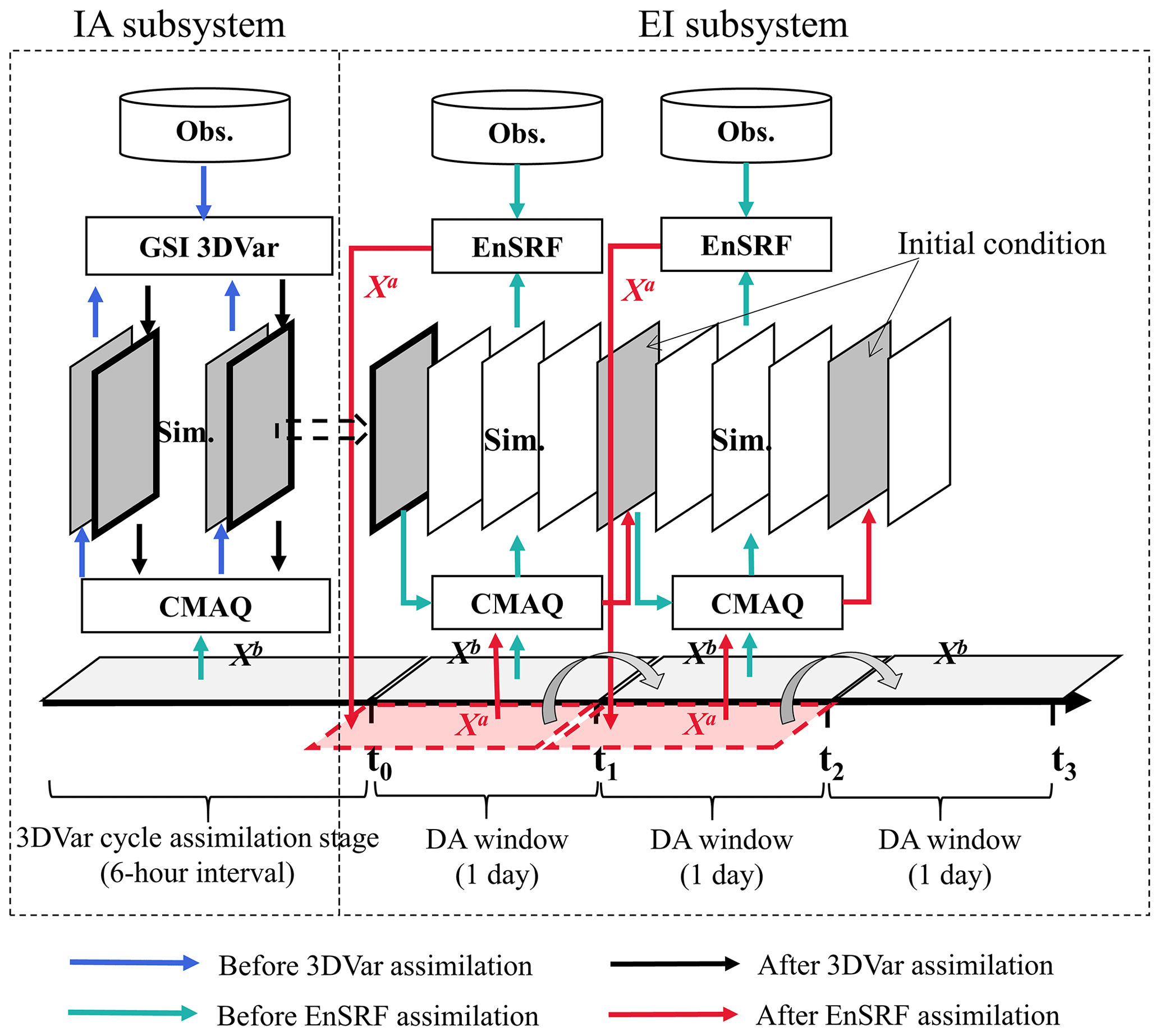
Figure 1 Composition and flowchart of RAPAS. X^a and X^b represent the prior and posterior emissions. The 3D-Var assimilation stage lasts 5 d with a data input frequency of 6 h, and the DA window in the EI subsystem is set to 1 d.

2.1.2 Atmospheric transport model

The regional chemical transport model of the Weather Research and Forecasting–Community Multiscale Air Quality (WRF–CMAQ) modeling system was adopted in this study (Skamarock and Klemp, 2008; Byun and Schere, 2006). CMAQ is a regional 3D Eulerian atmospheric chemistry and transport model with a “one-atmosphere” design developed by the US Environmental Protection Agency (EPA). It can simultaneously address the complex interactions among multiple pollutants as well as air quality issues. The CMAQ model was driven by the WRF model, which is a state-of-the-art mesoscale numerical weather prediction system designed for both atmospheric research and meteorological field forecasting. In this study, WRF version 4.0 and CMAQ version 5.0.2 were used. The WRF simulations were performed with a 36 km horizontal resolution on 169 × 129 grids, covering all of mainland China (Fig. 2). This spatial resolution has been widely adopted in regional simulations as it can provide good simulations of spatiotemporal variations in air pollutants (Mueller and Mallard, 2011; Sharma et al. 2016). In the vertical direction, there were 51 sigma levels on the sigma–pressure coordinates extending from the surface to 100 hPa. The underlying surface of the urban and built-up land was replaced by the MODIS land cover retrieval of 2016 to adapt to the rapid expansion of urbanization. The CMAQ model was run with the same domain but with three grid cells removed from each side of the WRF domain. There were 15 layers in the CMAQ vertical coordinates, which were interpolated from 51 WRF layers.

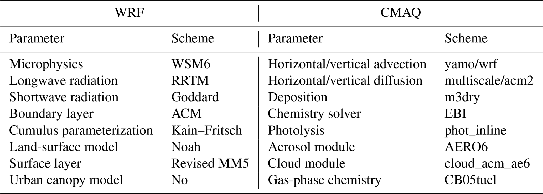
The meteorological initial and lateral boundary conditions were both provided by the final operational global analysis data of the National Centers for Environmental Prediction (NCEP) with a 1^∘ × 1^∘ resolution at 6 h intervals. The chemical lateral boundary conditions and chemical ICs in the IA subsystem originate from background profiles. As mentioned above, in the EI subsystem, the chemical IC in the first window is provided by the IA subsystem, and in the following windows, it is forward simulated using optimized emissions from the previous window. Carbon Bond 05 with updated toluene chemistry (CB05tucl) and the sixth-generation aerosol module (AERO6) were chosen as the gas-phase and aerosol chemical mechanisms, respectively (Appel et al., 2013; Sarwar et al., 2012). The detailed physical and chemical configurations are listed in Table 1.

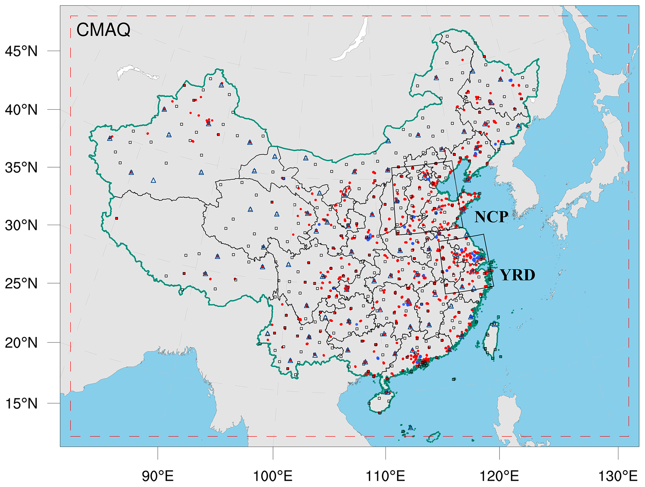
Figure 2 Model domain and observation network. The dashed red frame depicts the CMAQ computational domain, the black squares represent the surface meteorological measurement sites, the navy blue triangles represent the sounding sites, and the red and blue dots represent the air pollution measurement sites. Observations from all sites were assimilated in the 3D-Var subsystem, while observations of city sites where red dots were averaged are used for assimilation and where blue dots were averaged are used for independent evaluation in the EI subsystem; the boxed subregions are the North China Plain (NCP) and Yangtze River Delta (YRD), and the shaded area depicts the topography.

Table 1 Configuration options of Weather Research and Forecasting–Community Multiscale Air Quality model (WRF–CMAQ).

2.1.3 3D-Var assimilation algorithm

The Gridpoint Statistical Interpolation (GSI) system developed by the US NCEP was utilized in this study. Building on the work of Liu et al. (2011), Jiang et al. (2013b), and Feng et al. (2018), we extended the GSI to simultaneously assimilate multiple species (including CO, SO₂, NO₂, O₃, PM_2.5, and PM₁₀) and first used individual aerosol species of PM_2.5 as analysis variables within the GSI–WRF–CMAQ framework. Additional work includes the construction of surface air pollutant observation operators, the updating of observation errors, and the statistics of background error covariance for the analysis variables. Moreover, the data interface was modified to read/write the CMAQ output/input file directly, which was easy to implement.

In the sense of minimum analysis error variance, the 3D-Var algorithm optimizes the analysis fields with observations through an iterative process to minimize the cost function J(x) defined below:

$$\begin{array}{}\text{(1)}& \begin{array}{rl}J\left(x\right)& ={\displaystyle \frac{\mathrm{1}}{\mathrm{2}}}({\mathit{x}}_{\mathrm{a}}-{\mathit{x}}_{\mathrm{b}}{)}^{\mathrm{T}}{\mathbf{B}}^{-\mathrm{1}}({\mathit{x}}_{\mathrm{a}}-{\mathit{x}}_{\mathrm{b}})\\ & +{\displaystyle \frac{\mathrm{1}}{\mathrm{2}}}\left[\mathbf{H}\right({\mathit{x}}_{\mathrm{a}})-\mathit{y}{]}^{\mathrm{T}}{\mathbf{R}}^{-\mathrm{1}}[\mathbf{H}\left({\mathit{x}}_{\mathrm{a}}\right)-\mathit{y}],\end{array}\end{array}$$

where x_a is a vector of the analysis field; x_b is the background field; y is the vector of observations; B and R are the background and observation error covariance matrices, respectively, representing the relative contributions to the analysis; and H is the observation operator that maps the model variables to the observation space.

The analysis variables were the 3D mass concentrations of the pollution components (e.g., CO and sulfate) at each grid point. Hourly mean surface pollution observations within a 1 h window of the analysis were assimilated. To assimilate the surface pollution observations, model-simulated compositions were first diagnosed at observation locations. For gas concentrations to be directly used as analysis variables, the units need to be converted from parts per million (ppm) and parts per billion (ppb) to milligrams per cubic meter (mg m⁻³) and micrograms per cubic meter (µg m⁻³), respectively, to match the observations. The model-simulated PM_2.5 and PM₁₀ concentrations at the ground level were diagnosed as follows:

$$\begin{array}{}\text{(2)}& {\displaystyle }\begin{array}{rl}{\mathrm{PM}}_{\mathrm{2.5}}& =f_i\times {\mathrm{PM}}_i+f_j\times {\mathrm{PM}}_j+f_k\times {\mathrm{PM}}_k=\mathrm{OC}\\ & +\mathrm{EC}+{\mathrm{SO}}_{\mathrm{4}}^{\mathrm{2}-}+{\mathrm{NO}}_{\mathrm{3}}^{-}+{\mathrm{NH}}_{\mathrm{4}}^{+}+\mathrm{SEAS}+{\mathrm{AP}}_{\mathrm{2.5}},\end{array}\text{(3)}& {\displaystyle }{\mathrm{PM}}_{\mathrm{10}}={\mathrm{PM}}_i+{\mathrm{PM}}_j+{\mathrm{PM}}_k={\mathrm{PM}}_{\mathrm{2.5}}+\mathrm{PMC},\end{array}$$

where f_i, f_j, and f_k are the PM_2.5 fractions of the Aitken, accumulation, and coarse modes, respectively. These ratios are recommended as the concentrations of PM_2.5 and fine-mode aerosols (i.e., Aitken plus accumulation) can differ because PM_2.5 particles include small tails from the coarse mode in the CMAQ model (Binkowski and Roselle, 2003; Jiang et al., 2006). PM_i, PM_j, and PM_k are the mass concentrations of the Aitken, accumulation, and coarse modes in the CMAQ model, respectively. Seven aerosol species of PM_2.5 (organic carbon (OC), elemental carbon (EC), sulfate (SO${}_{\mathrm{4}}^{\mathrm{2}-}$), nitrate (NO${}_{\mathrm{3}}^{-}$), ammonium (NH${}_{\mathrm{4}}^{+}$), sea salt (SEAS), and fine-mode unspeciated aerosols (AP_2.5)) and additional coarse PM₁₀ (PMC) were extracted as analysis variables and were updated using the PM_2.5 and PMC observations. Before calculating Eq. (1) within the GSI, the analysis variables were bilinearly interpolated in the horizontal direction to the observation locations.

Calculating background error covariance (B) is generally costly and difficult when a high-dimensional numerical model is used. For simplification, B was represented as a product of spatial correlation matrices and standard deviations (SDs):

$$\begin{array}{}\text{(4)}& {\displaystyle }\mathbf{B}={\mathbf{DCD}}^{\mathrm{T}}\text{(5)}& {\displaystyle }\mathbf{C}={\mathbf{C}}_x\otimes {\mathbf{C}}_y\otimes {\mathbf{C}}_z,\end{array}$$

where D is the background error SD matrix; C is the background error correlation matrix; ⊗ is the Kronecker product; and C_x, C_y, and C_z denote three 1D correlation submatrices in the longitude, latitude, and vertical coordinate directions, respectively. C_x and C_y are assumed to be horizontally isotropic such that they can be represented using a Gaussian function. The correlation between any two points x_i and x_j in the horizontal direction is expressed as follows:

$$\begin{array}{}\text{(6)}& c\left(x_i,x_j\right)=e^{-\frac{(x_i-x_j{)}^{\mathrm{2}}}{\mathrm{2}{L}^{\mathrm{2}}}},\end{array}$$

where L is the horizontal correlation scale estimated using the proxy of the background error (Fig. 3). The vertical correlation matrix C_z is directly estimated from the model background field as C_z is only an n_z×n_z (here, n_z=15) matrix.

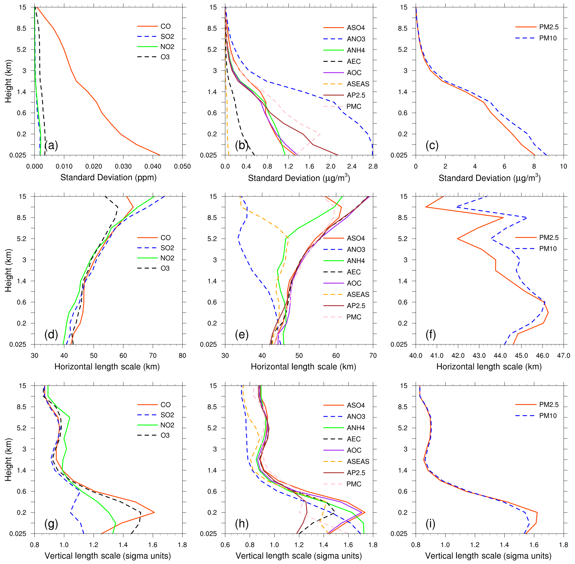
Figure 3 Vertical profiles of standard deviations (a, ppm; b and c, µg m⁻³) and horizontal (d–f, km) and vertical (g–i, sigma units) length scales for CO, SO₂, NO₂, O₃, sulfate, nitrate, ammonium, EC, OC, sea salt, unspeciated aerosols (AP_2.5), PMC, PM_2.5, and PM₁₀.

To estimate these matrices, the National Meteorological Center (NMC) method was used to compute B for each variable by taking the differences between forecasts of different lengths valid at the same time (Parrish and Derber, 1992; Rabier et al., 1998). Differences between the 24 and 12 h WRF–CMAQ forecasts of 60 pairs (2 pairs per day) of analysis variables valid at either 00:00 or 12:00 UTC during November 2016 were used. The horizontal and vertical length scales of the correlation matrices were estimated using recursive filters (Purser et al., 2003). The vertical distribution of the background error SDs, which varies with height and species, is shown in Fig. 3. The vertical profile of the background error SDs corresponds to the vertical concentration distribution. This means that higher concentrations tend to have larger background error SDs (e.g., CO and nitrate). These SDs exhibit a common reduction as the height increases, especially at the top of the boundary layer. The horizontal correlation of the background error determines the propagation of observation information in this direction, whereas the vertical correlation determines the vertical extension of such increments. For gaseous pollutants and most individual aerosol components, the horizontal length scales increased with height, whereas for the total particulate matter (i.e., PM_2.5, PM₁₀), the scales increased with height in the boundary layer and decreased with height in the free troposphere. The ground-level scale generally spreads across 40–45 km for all control variables. The vertical length scale of most species first increased and then decreased with height, which may be related to vertical mixing (Kahnert, 2008) and stack emissions at approximately 200 m height.

2.1.4 EnKF assimilation algorithm

In EnKF, the time-dependent uncertainties of the state variables are estimated using a Monte Carlo approach through an ensemble. Uncertainty can be propagated using linear or nonlinear dynamic models (flow-dependent background error covariance) by simply implementing ensemble simulations. The EnSRF algorithm introduced by Bierman (1977) and Maybeck (1979) was used to constrain pollution emissions in this study. EnSRF is a deterministic EnKF that obviates the need to perturb observations, which has a higher computational efficiency and a better performance (Sun et al., 2009).

The perturbation of the prior emissions represents the uncertainty. We implemented additive emission adjustment methods, which were calculated using the following function:

$$\begin{array}{}\text{(7)}& {\mathbf{X}}_i^{\mathrm{b}}={\mathbf{X}}_{\mathrm{0}}^{\mathrm{b}}+\mathit{\delta }{\mathbf{X}}_i^{\mathrm{b}},i=\mathrm{1},\mathrm{2},\mathrm{\dots },N,\end{array}$$

where b is the background (prior) state; i is the identifier of the perturbed samples; and N is the ensemble size, which was set to 40 considering the trade-off between computational cost and inversion accuracy (Fig. S1). In contrast to the estimation of parameters based on the augmentation of the conventional state vector (e.g., concentrations) with the parameter variables, X only comprises emissions in this study (similarly hereafter). $\mathit{\delta }{\mathbf{X}}_i^{\mathrm{b}}$ is the randomly perturbed samples added to the prior emissions ${\mathbf{X}}_{\mathrm{0}}^{\mathrm{b}}$ to produce ensemble samples of the inputs ${\mathbf{X}}_i^{\mathrm{b}}$. $\mathit{\delta }{\mathbf{X}}_i^{\mathrm{b}}$ is drawn from Gaussian distributions with a mean of 0 and standard deviation of the prior emission uncertainty in each grid. The state variables of the emissions include CO, SO₂, NO_x, primary PM_2.5 (PPM_2.5), and PMC. We used variable localization to update the analysis, which means that the covariance among different state variables was not considered, and the emission of one species was constrained only by its corresponding air pollutant observation. This method has been widely used in chemical data assimilation systems to avoid spurious correlations between species (Ma et al., 2019; Miyazaki et al., 2012b).

After obtaining an ensemble of state vectors (prior emissions), ensemble runs of the CMAQ model were conducted to propagate the errors in the model with each ensemble sample of state vectors. Combined with the observational vector y, the state vector $\stackrel{\mathrm{‾}}{{\mathbf{X}}^{\mathrm{b}}}$ was updated by minimizing the analysis variance.

$$\begin{array}{}\text{(8)}& {\displaystyle }\stackrel{\mathrm{‾}}{{\mathbf{X}}^{\mathrm{a}}}=\stackrel{\mathrm{‾}}{{\mathbf{X}}^{\mathrm{b}}}+\mathbf{K}(\mathit{y}-\mathbf{H}\stackrel{\mathrm{‾}}{{\mathbf{X}}^{\mathrm{b}}}),\text{(9)}& {\displaystyle }\mathbf{K}={\mathbf{P}}^{\mathrm{b}}{\mathbf{H}}^{\mathrm{T}}({\mathbf{HP}}^{\mathrm{b}}{\mathbf{H}}^{\mathrm{T}}+\mathbf{R}{)}^{-\mathrm{1}},\text{(10)}& {\displaystyle }{\mathbf{P}}^{\mathrm{b}}={\displaystyle \frac{\mathrm{1}}{N-\mathrm{1}}}{\sum }_{i=\mathrm{1}}^N({\mathbf{X}}_i^{\mathrm{b}}-\stackrel{\mathrm{‾}}{{\mathbf{X}}^{\mathrm{b}}})({\mathbf{X}}_i^{\mathrm{b}}-\stackrel{\mathrm{‾}}{{\mathbf{X}}^{\mathrm{b}}}{)}^{\mathrm{T}},\text{(11)}& {\displaystyle }\mathit{\delta }{\mathbf{X}}_i^{\mathrm{a}}=\mathit{\delta }{\mathbf{X}}_i^{\mathrm{b}}-\stackrel{\mathrm{̃}}{\mathbf{K}}\mathbf{H}\mathit{\delta }{\mathbf{X}}_i^{\mathrm{b}}\end{array}$$

While employing sequential assimilation and independent observations, $\stackrel{\mathrm{̃}}{\mathbf{K}}$ is calculated as follows:

$$\begin{array}{}\text{(12)}& \stackrel{\mathrm{̃}}{\mathbf{K}}={\left(\mathrm{1}+\sqrt{\mathbf{R}/\left({\mathbf{HP}}^{\mathrm{b}}{\mathbf{H}}^{\mathrm{T}}+\mathbf{R}\right)}\right)}^{-\mathrm{1}}\mathbf{K},\end{array}$$

where $\stackrel{\mathrm{‾}}{{\mathbf{X}}^{\mathrm{b}}}$ is the mean of the ensemble samples ${\mathbf{X}}_i^{\mathrm{b}}$; H is the observation operator that maps the model space to the observation space, consisting of the model integration process converting emissions into concentrations and spatial interpolation matching the model concentration to the locations of the observations; $\mathit{y}-\mathbf{H}\stackrel{\mathrm{‾}}{{\mathbf{X}}^{\mathrm{b}}}$ reflects the differences between the simulated and observed concentrations; P^b is the ensemble-estimated background (a priori) error covariance; K is the Kalman gain matrix of the ensemble mean depending on the background error covariance P^b and the observation error covariance R, representing the relative contributions to analysis; and $\stackrel{\mathrm{̃}}{\mathbf{K}}$ is the Kalman gain matrix of the ensemble perturbation, which is used to calculate emission perturbations after inversions $\mathit{\delta }{\mathbf{X}}_i^{\mathrm{a}}$. The ensemble mean $\stackrel{\mathrm{‾}}{{\mathbf{X}}^{\mathrm{a}}}$ of the analyzed state was considered the best estimate of the emissions.

When large volumes of site observations are at a much higher resolution than the model grid spacing, many correlated or fully consistent model–data mismatch errors can appear in one cluster, resulting in excessive adjustments and deteriorated model performance (Houtekamer and Mitchell, 2001). To reduce the horizontal observation error correlations and influence of representativeness errors, a super-observation approach combining multiple noisy observations located within the same grid and assimilation window was developed based on optimal estimation theory (Miyazaki et al., 2012a). Previous studies have demonstrated the necessity for data-thinning and dealiasing errors (Feng et al., 2020b; Zhang et al., 2009a). The super-observation y_new, super-observation error r_new, and corresponding simulation x_new,i of the ith sample are calculated as follows:

$$\begin{array}{}\text{(13)}& {\displaystyle }\mathrm{1}/r_{\mathrm{new}}^{\mathrm{2}}={\sum }_{j=\mathrm{1}}^m\mathrm{1}/r_j^{\mathrm{2}},\text{(14)}& {\displaystyle }{y}_{\mathrm{new}}={\sum }_{j=\mathrm{1}}^m{w}_j{y}_j/{\sum }_{j=\mathrm{1}}^m{w}_j,\text{(15)}& {\displaystyle }{x}_{\mathrm{new},i}={\sum }_{j=\mathrm{1}}^m{w}_j{x}_{ij}/{\sum }_{j=\mathrm{1}}^m{w}_j,\end{array}$$

where j is the identifier of m observations within a super-observation grid, r_j is the observational error of the actual jth observation y_j, x_ij is the simulated concentration using the ith prior emission sample corresponding to the jth observation, and $w_j=\mathrm{1}/r_j^{\mathrm{2}}$ is the weighting factor. The super-observation error decreased as the number of observations used within a super-observation increased. This method was used in our previous inversions using surface-based (Feng et al., 2020b) and satellite-based (Jiang et al., 2021) observations.

In this study, the DA window was set to 1 d because the model requires a longer time to integrate the emission information into the concentration ensembles (Ma et al., 2019). Due to the super-observation approach, only one assimilation is needed per grid cell in one assimilation window. In addition, owing to the complexity of hourly emissions, it is difficult to simulate hourly concentrations that match the observations well. Although a longer DA window would allow more observations to constrain the emission change of one grid, the spurious correlation signals of EnKF would attenuate the observation information over time (Bruhwiler et al., 2005; Jiang et al., 2021). Kang et al. (2012) conducted observing system simulation experiments (OSSEs) and demonstrated that owing to the transport errors and increased spurious correlation, a longer DA window (e.g., 3 weeks) would cause the analysis system to blur essential emission information away from the observation. Therefore, daily mean simulations and observations were used in the EnSRF algorithm, and daily emissions were optimized in this system.

EnKF is subject to spurious correlations because of the limited number of ensembles when it is applied in high-dimensional atmospheric models, which can cause rank deficiencies in the estimated background error covariance and filter divergence as well as further degrade analyses and forecasts (Wang et al., 2020). Covariance localization is performed to reduce spurious correlations caused by a finite ensemble size (Houtekamer and Mitchell, 2001). Covariance localization preserves the meaningful impact of observations on state variables within a certain distance (cutoff radius) but limits the detrimental impact of observations on remote state variables. The localization function of Gaspari and Cohn (Gaspari and Cohn, 1999) is used in this system, which is a piecewise continuous fifth-order polynomial approximation of a normal distribution. The optimal localization scale is related to the ensemble size, assimilation window, dynamic system, and lifetime of the chemical species in the atmosphere. CO, SO₂, and PM_2.5 are rather stable in the atmosphere, with a lifetime of more than 1 d. According to the average wind speed (3.3 m s⁻¹, Table 4) and length of the DA window, the localization scales of CO, SO₂, and PM_2.5 were set to 300 km. In addition, the localization scales of NO₂, which is rather reactive and has a lifetime of approximately 10 h in winter (de Foy et al., 2015), and PMC, which mainly comes from local sources and has a short residence time in the atmosphere owing to the rapid deposition rate (Clements et al., 2014, 2016; Hinds, 1982), were set to 150 and 250 km, respectively.

2.2 Prior emissions and uncertainties

Anthropogenic emissions over China were obtained from the 2016 Multi-resolution Emission Inventory for China (MEIC 2016) (Zheng et al., 2018), while those over the other regions of eastern Asia were obtained from the mosaic Asian anthropogenic emission inventory (MIX) (Li et al., 2017). The spatial resolutions of the MEIC and MIX inventories were both 0.25^∘ × 0.25^∘, and they are downscaled to match the model grid spacing of 36 km. The spatial distributions of CO, SO₂, NO_x, PPM_2.5, and PMC emissions are shown in Fig. 12. The daily emission inventory, which was arithmetically averaged from the combined monthly emission inventory, was directly used in the EI subsystem and was employed as the prior emission of the first DA window in the EI subsystem (Fig. 1). During the simulations, daily emissions were further converted to hourly emissions. All species emitted from area sources were converted to hourly emissions using the same diurnal profile (Fig. S2), and for the point source, we assumed that there was no diurnal change. MEIC 2012 was used as an alternative a priori over China to investigate the impact of different prior emissions on optimized emissions. The Model of Emissions of Gases and Aerosols from Nature (MEGAN) (Guenther et al., 2012) was used to calculate time-dependent biogenic emissions, which was driven by the WRF model. Biomass burning emissions were not included because they have little impact across China during the study period (Zhang et al., 2020).

During the inversion cycles, inverted emissions of different members converge gradually, and the ensemble-estimated error covariance matrix is likely to be underestimated. To avoid this, considering the compensation of model errors and comparable emission uncertainties from one day to the next, we imposed the same uncertainty on emissions at each DA window. As mentioned above, the optimized emissions of the current DA window were transferred to the next DA window as prior emissions. The technology-based emission inventory developed by Zhang et al. (2009b), using the same method as MEIC, showed that the emissions of PMC and PPM_2.5 had the largest uncertainties, followed by CO and finally SO₂ and NO_x. Therefore, the uncertainties in PMC, PPM_2.5, CO, SO₂, and NO_x in this study were set as 40 %, 40 %, 30 %, 25 %, and 25 %, respectively. However, previous studies have shown that inversely estimated CO and PMC emissions can exceed 100 % higher than the bottom-up emissions (MEIC) in certain areas (Feng et al., 2020b; Ma et al., 2019). Therefore, according to the extent of underestimation, we set an uncertainty of 100 % for both the CO and the PMC emissions at the beginning of the three DA windows to quickly converge the emissions. Mean emission analysis is generally minimally sensitive to the uncertainty setting in the assimilation cycle method (Feng et al., 2020a; Gurney et al., 2004; Miyazaki et al., 2012a) as the inversion errors of the current window can be transferred to the next window for further optimization (Sect. 4.3).

2.3 Observation data and errors

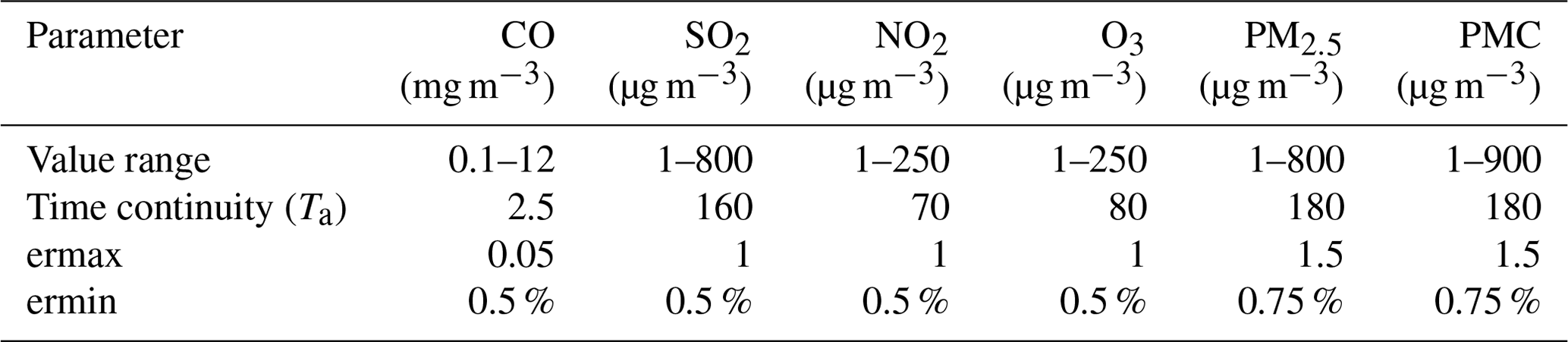
Hourly-averaged surface CO, SO₂, NO₂, O₃, PM_2.5, and PM₁₀ observations from 1504 national air quality monitoring stations were assimilated into this system, which were obtained from the Ministry of Ecology and Environment of the People's Republic of China (https://air.cnemc.cn:18007/, last access: 25 June 2020). These sites are distributed over most of central and eastern China and become denser near metropolitan areas (see Fig. 2). To ensure data quality, value-range checks were performed to eliminate unrealistic or unrepresentative observations, and only the observations within the subjectively selected threshold range were assimilated (Table 2). In addition, a time-continuity check was performed to eliminate gross outliers and sudden anomalies using the function $max\left(\left|O\left(t\right)-O\left(t\pm \mathrm{1}\right)\right|\right)\le f(t$), where O(t) and O(t±1) represent observations at time t and t±1, respectively, and $f\left(t\right)=T_{\mathrm{a}}+T_{\mathrm{b}}\times O_t$. This means that the concentration difference between time t and time t+1 and time t−1 should be less than f(t). T_b was fixed at 0.15, and the section of T_a is given in Table 2, which was determined empirically according to the time series change in the concentration at each site. To avoid potential cross-correlations, we assimilated PM_2.5 and PMC. Additionally, in the EI subsystem, the observations within each city were averaged to reduce the data density, reduce the error correlation, and increase spatial representation (Houtekamer and Mitchell, 2001; Houtekamer and Zhang, 2016). Finally, 336 city sites were available across mainland China, in which data from 311 cities were selected for assimilation, and the remaining 25 were selected for independent validation (Fig. 2). In the IA subsystem, owing to the small horizontal correlation scale (Fig. 3), all site observations were assimilated to provide a good IC for the next emission inversion in order to obtain more extensive observation constraints.

The observation error covariance matrix (R) includes both the measurement and the representation errors. The measurement error ε₀ is defined as follows:

$$\begin{array}{}\text{(16)}& {\mathit{\epsilon }}_{\mathrm{0}}=\mathrm{ermax}+\mathrm{ermin}\times {\mathrm{\Pi }}_{\mathrm{0}},\end{array}$$

where ermax is the base error, and Π₀ denotes the observed concentration. These parameters for different species are listed in Table 2 and were determined according to Chen et al. (2019), Feng et al. (2018), and Jiang et al. (2013b).

The representative error depends on the model resolution and characteristics of the observation locations, which were calculated using the equations of Elbern et al. (2007), defined as follows:

$$\begin{array}{}\text{(17)}& {\mathit{\epsilon }}_{\mathrm{r}}=\mathit{\gamma }{\mathit{\epsilon }}_{\mathrm{0}}\sqrt{\mathrm{\Delta }l/L},\end{array}$$

where γ is a tunable parameter (here, γ=0.5), Δl is the grid spacing (36 km), and L is the radius (3 km for simplification) of the influence area of the observation. The total observation error (r) was defined as follows:

$$\begin{array}{}\text{(18)}& r=\sqrt{{\mathit{\epsilon }}_{\mathrm{0}}^{\mathrm{2}}+{\mathit{\epsilon }}_{\mathrm{r}}^{\mathrm{2}}}.\end{array}$$

Table 2 Parameters of quality control and measurement error.

3 Experimental design

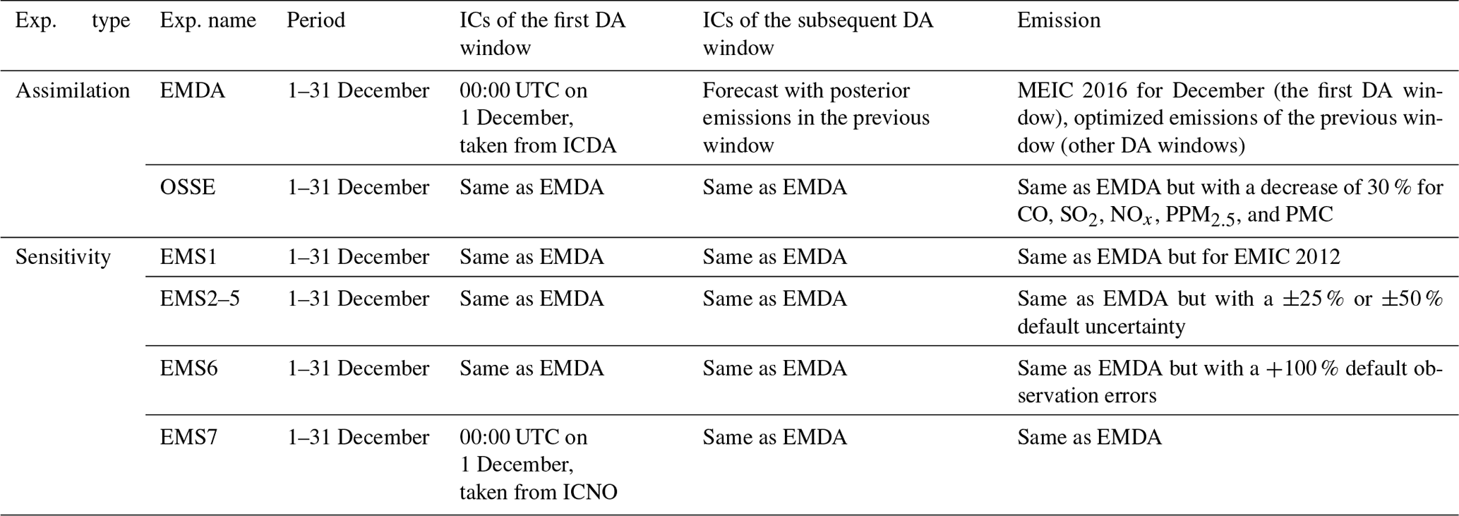
RAPAS inversions were conducted according to the procedure and settings described in Sect. 2. December is one of the months with the most severe air pollution, whereas July is one of the least polluted months in China. Therefore, this study mainly tested the performance of the RAPAS system over these 2 months. For December, the IA subsystem was run from 26 to 30 November 2016, with a 6 h interval cycling assimilation to optimize ICs (ICDA). A better IC at 00:00 UTC on 1 December could be obtained by a 5 d high-frequency cycling assimilation and atmospheric mixing. The EI subsystem was then run for December 2016 with a 1 d assimilation window to optimize emissions (EMDA). In July, the system operated identically to that of December. It should be noted that owing to the stronger atmospheric oxidation, the lifetime of NO₂ in July was significantly shorter than that in December; thus, we adopted a smaller localization scale for NO₂ (80 km). Both assimilation experiments used the combined prior emission inventories of 2016, as described in Sect. 2.2, and the emission base year coincided with the research stage. An observing system simulation experiment (OSSE) was conducted to evaluate the performance of the RAPAS system, which has been widely used in previous assimilation system developments (Daley, 1997). In the OSSE experiment, we used the MEIC 2016 inventory as a “true” emission and the true emission, reduced by 30 % over mainland China, as a prior emission. The simulations were performed using the true emission and sampled according to the locations and times of the real observations used as artificial observations. The observation errors were the same as those in EMDA. To evaluate the IC improvements from the IA subsystem, an experiment without 3D-Var (NODA) was conducted with the same meteorological fields and physical and chemistry parameterization settings as those of the ICDA. To evaluate the posterior emissions of the EI subsystem, two parallel forward-modeling experiments were performed for December 2016: a control experiment (CEP) with prior (MEIC 2016) emissions and a validation experiment (VEP) with posterior emissions. Both experiments used the same IC at 00:00 UTC on 1 December generated through the IA subsystem. The only difference between CEP and VEP were emissions. Table 3 summarizes the different emission inversion experiments conducted in this study.

To investigate the robustness of our system, seven sensitivity tests (from EMS1 to EMS7; see Table 3) were performed. These experiments were all based on EMDA. EMS1 used MEIC 2012 as the original prior emission in China, aiming to investigate the impact of different prior inventories on the estimates of emissions. The other experiments (EMS2–5) aimed to test the impact of different prior uncertainty settings, in which the prior uncertainties were reduced by −50 % and −25 % and increased by 25 % and 50 %, respectively. EMS6 aimed to evaluate the impact of observation errors on emission estimates, in which all observation errors are magnified twice. EMS7 aimed to evaluate the impact of IC optimization of the first window on emission estimates, in which the ICs were taken from a 5 d spin-up simulation. Eight forward-modeling experiments (VEP1, VEP2, …, VEP7) were also performed with the posterior emissions of EMS1 to EMS7 to evaluate their performance.

Table 3 Emission inversion and sensitivity experiments conducted in this study.

4 Results

4.1 Evaluations

4.1.1 Simulated meteorological fields

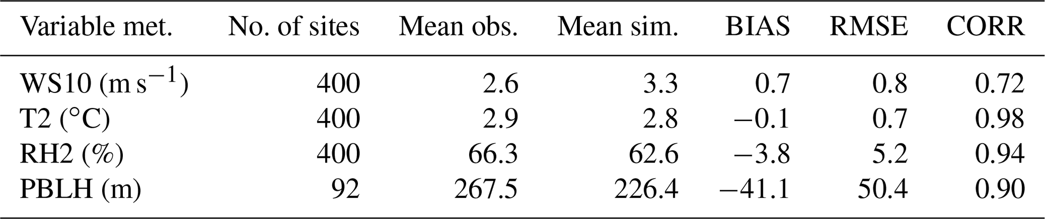
In the RAPAS system, the inversion approach attributes all biases between the simulated and observed concentrations to emissions. Meteorological fields dominate the physical and chemical processes of air pollutants in the atmosphere, and thus their simulation accuracy would significantly affect the estimates of emissions in this study. To quantitatively evaluate the performance of the WRF simulations, the mean bias (BIAS), root mean square error (RMSE), and correlation coefficient (CORR) were calculated against the surface meteorological observations measured at 400 stations, and the planetary boundary layer height (PBLH) was calculated using the sounding data at 92 sites. Surface observations were obtained from the National Climatic Data Center integrated surface database (http://www.ncdc.noaa.gov/oa/ncdc.html, last access: 25 October 2021), and sounding data were obtained from the website of the University of Wyoming (http://weather.uwyo.edu/upperair/sounding.html, last access: 10 March 2022). The sounding data had a 12 h interval. The observed PBLH was calculated using sound data via the bulk Richardson number method (Richardson et al., 2013). The spatial distribution of meteorological stations is shown in Fig. 2. The simulated temperature at 2 m (T2), relative humidity at 2 m (RH2), wind speed at 10 m (WS10), and PBLH from 26 November to 31 December 2016 were evaluated against the observations. Table 4 summarizes the statistical results of the evaluation of the simulated meteorological parameters. Overall, T2, RH2, and PBLH were slightly underestimated, with biases of −0.1 ^∘C, −3.8 %, and −41.1 m, respectively. CORRs were approximately 0.98 for T2, 0.94 for RH2, and 0.90 for PBLH, showing good consistency between the observations and simulations. WS10 was overestimated, with a bias of 0.7 m s⁻¹ and an RMSE of 0.8 m s⁻¹ but was better than the simulations from many previous studies (Chen et al., 2016; Jiang et al., 2012a, b). Therefore, the WRF can generally reproduce meteorological conditions sufficiently in terms of their temporal variation and magnitude over China, which is adequate for our inversion estimation.

Table 4 Statistics comparing the simulated and observed 10 m wind speed (WS10), 2 m temperature (T2), and 2 m relative humidity (RH2), as well as the planetary boundary layer height (PBLH). BIAS: mean bias; RMSE: root mean square error; CORR: correlation coefficient.

4.1.2 Initial conditions

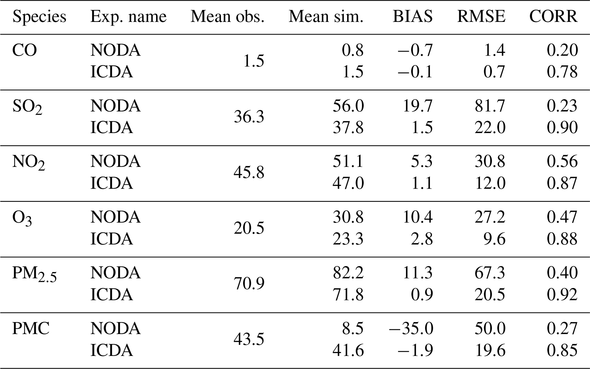
Figure 4 shows an evaluation of the analyzed concentrations of the six species against surface observations. For comparison, the evaluations of the simulations without 3D-Var (NODA) are also shown in Fig. 4. The simulations of the NODA experiment (red dots) are scattered on both sides of the central line, as large systematic biases remain across many measurement sites. Conversely, the ICDA experiment (blue dots) showed a much better agreement with the observations than those from NODA. The statistics show that there are large systematic biases in the NODA simulations, with large RMSEs and small CORRs for all species, particularly for CO and PMC. After the assimilation of surface observations, the RMSE of CO decreased to 0.7 mg m⁻³, and the RMSEs of SO₂, NO₂, O₃, PM_2.5, and PMC decreased to 22.0, 12.0, 9.6, 20.5, and 19.6 µg m⁻³, respectively, with respective reductions of 50.0 %, 73.1 %, 61.0 %, 64.7 %, 69.5 %, and 60.8 % compared to those of NODA (Table 5). The CORRs of ICDA increased by 290.0 %, 291.3 %, 55.4 %, 87.2 %, 130.0 %, and 214.8 % to 0.78, 0.90, 0.87, 0.88, 0.92, and 0.85, respectively. These statistics indicate that the ICs of the ground level improved significantly. However, owing to the lack of observations, we still do not know the simulation bias in the upper–middle boundary layer. Although concentrations at high altitudes can be constrained by ground-based observations through vertical correlations, the effect is limited; therefore, the bias remains non-negligible.

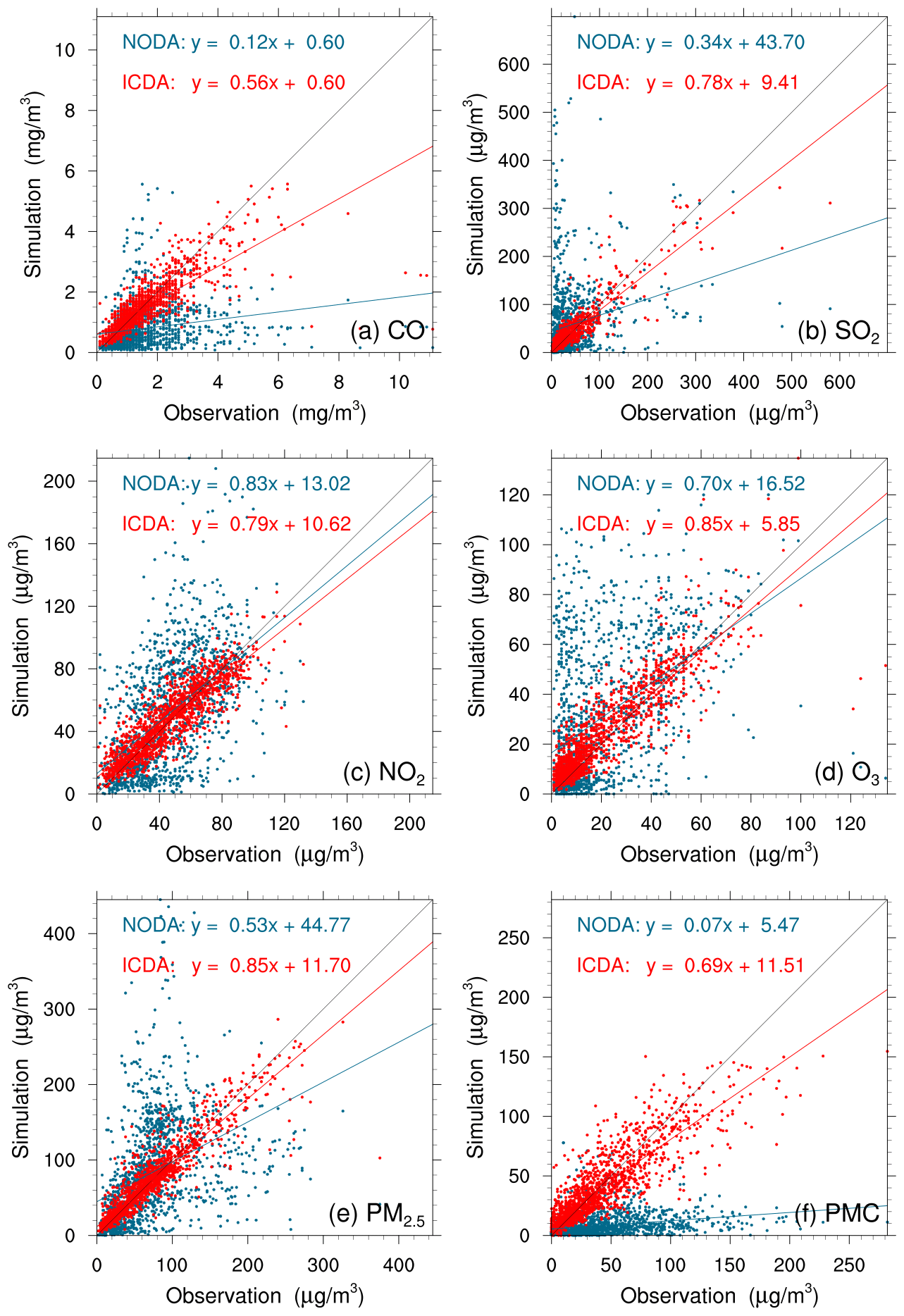
Figure 4 Scatterplots of simulated versus observed (a) CO, (b) SO₂, (c) NO₂, (d) O₃, (e) PM_2.5, and (f) PMC mass concentration initializations from the background (red) and analysis (blue) fields at 00:00 UTC on 1 December.

Table 5 Comparisons of the surface CO, SO₂, NO₂, O₃, PM_2.5, and PMC mass concentrations from the control and assimilation experiment against observations aggregated over all analysis times. CO unit: mg m⁻³; other units: µg m⁻³. BIAS: mean bias; RMSE: root mean square error; CORR: correlation coefficient.

4.1.3 Posterior emissions

Owing to the mismatched spatial scales, it is difficult to directly evaluate the optimized emissions against observations. Generally, we indirectly validated the optimized emissions by comparing the forward-simulated concentrations using the posterior emissions against atmospheric measurements (e.g., Jiang et al., 2014; Jin et al., 2018; Peters et al., 2007). Figure 5 shows the spatial distributions of the mean biases between the gaseous pollutants simulated using prior and posterior emissions and assimilated observations. In the CEPs, for each species, the distribution of biases was similar to the increments in background fields constrained through 3D-Var, as shown in Fig. S3. For example, almost all sites had large negative biases for CO, while for SO₂ and NO₂, positive biases were mainly distributed over the North China Plain (NCP), the Yangtze River Delta (YRD), the Sichuan Basin (SCB), and central China, and negative biases were distributed over the remaining areas. After constraining with observations, the biases of all three gaseous air pollutants were significantly reduced at most sites. For CO, the biases at 62 % of the sites decreased to absolute values less than 0.2 mg m⁻³, and for SO₂ and NO₂, the biases at 52 % and 47 % of the sites were within ±4 µg m⁻³. However, large negative biases were still observed in western China, indicating that the uncertainties of the posterior emissions are still large in western China, which may be attributed to the large biases in prior emissions and the relatively limited observations. Overall, the statistics show that there are different levels of improvement at the 311 assimilation sites of 92 %, 85 %, and 85 % for CO, SO₂, and NO₂, respectively. The small number of sites with a worse performance may be related to over-adjusted emissions by EI or contradictory adjustments caused by opposite biases in adjacent areas.

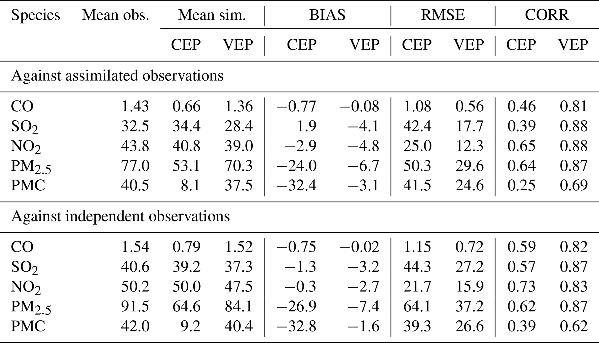
Table 6 lists the statistical results of the evaluations averaged over the whole mainland of China. For CO, the mean bias was −0.8 mg m⁻³ with the prior emissions, while it substantially reduced to −0.1 mg m⁻³ (reduction rate of 89.6 %) when simulating with the posterior emissions. Additionally, the RMSE decreased by 48.1 % from 1.08 to 0.56 mg m⁻³, and the CORR increased by 76.1 % from 0.46 to 0.81. For SO₂ and NO₂, the regional mean biases increased slightly as the positive/negative biases among different sites might be offset. However, the RMSEs decreased to 17.7 and 12.3 µg m⁻³, respectively, which were 58.3 % and 50.8 % lower than those of CEPs, and the CORRs increased by 125.6 % and 35.4 %, both reaching up to 0.88, indicating that EI significantly improved the NO_x and SO₂ emission estimates.

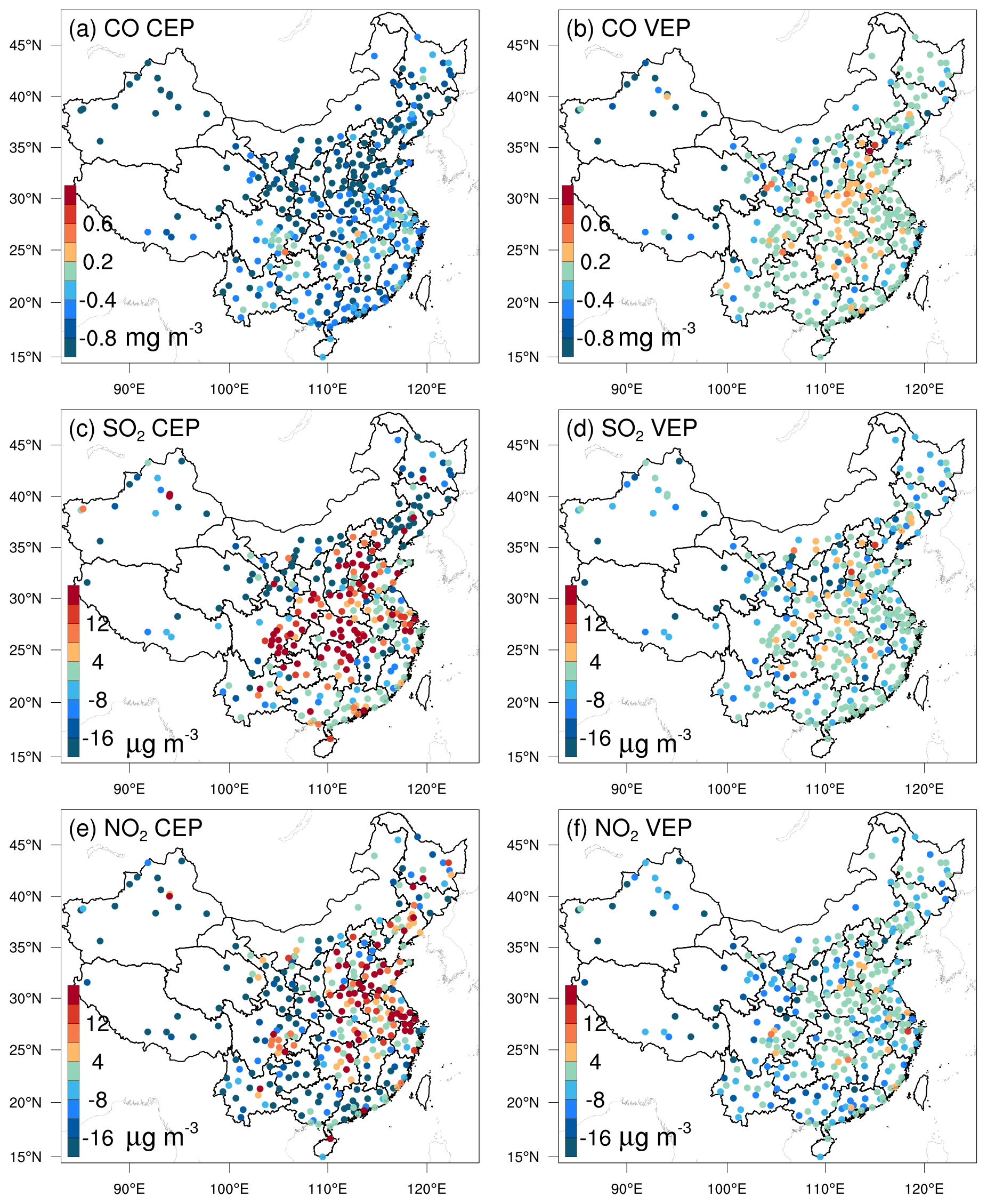
Figure 5 Spatial distribution of the BIAS of the simulated (a, b) CO, (c, d) SO₂, and (e, f) NO₂ with prior (a, c, e, CEP) and posterior (b, d, f, VEP) emissions. CO unit: mg m⁻³; SO₂ and NO₂ units: µg m⁻³.

Figure 6 shows the spatial distributions of the mean biases of simulated PM_2.5 and PMC evaluated against assimilated observations. Similarly, the CEP simulations did not perform well. There were widespread underestimations across the country, with mean biases of −24.0 and −32.4 µg m⁻³. After data assimilation, the performance of the VEP simulations significantly improved. The biases decreased by 72.1 % and 90.4 % to −6.7 and −3.1 µg m⁻³; the RMSEs decreased by 41.2 % and 40.7 % to 29.6 and 24.6 µg m⁻³; and the CORRs increased by 35.9 % and 176.0 % to 0.87 and 0.69 for PM_2.5 and PMC, respectively. Overall, 89.6 % and 97.2 % of the assimilation sites were improved for PM_2.5 and PMC, respectively. However, compared with the results for the three gaseous pollutants, there were sites with large biases scattered throughout the entire domain. In addition to the potential over-adjusted or contradictory adjustments of emissions as in the three gas species, the sites with large biases may be related to the complex precursors and complex homogeneous and heterogeneous chemical reactions and transformation processes of secondary PM_2.5 and the fact that we did not simulate the time variation in dust blowing caused by wind speed for PMC owing to the lack of land cover data that are compatible with the CMAQ dust module and agricultural activity data to identify dust source regions.

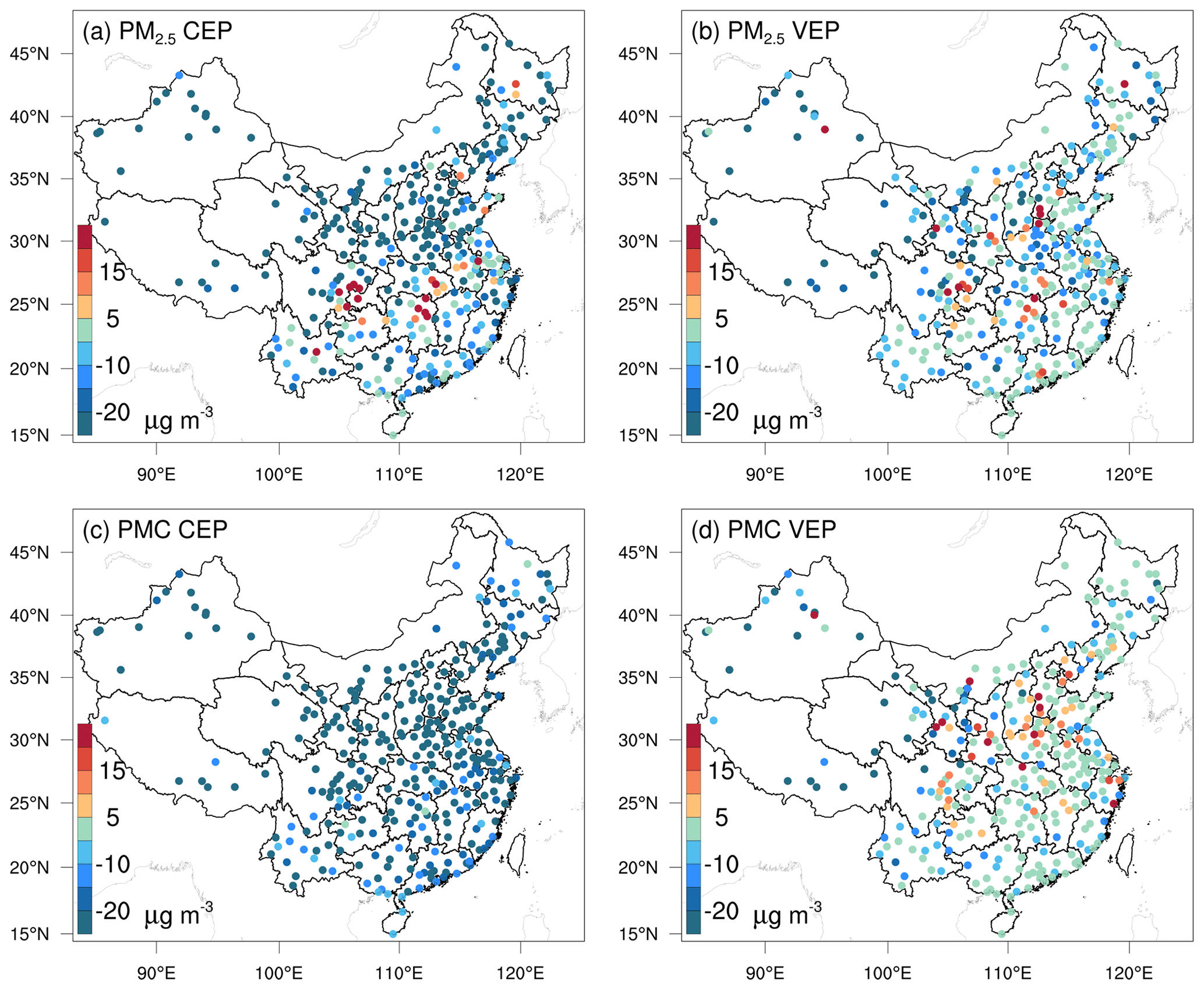
Figure 6 The same as in Fig. 5 but for PM_2.5 and PMC.

Figures 7 and 8 show the spatial distributions of the biases calculated against independent observations for the five species. With posterior emissions, the decreasing ratios of RMSEs ranged from 26.7 %–42.0 %, and the CORRs increased by 13.7 %–59.0 % to 0.62–0.87. Overall, the biases at the independent sites are similar or slightly worse than those at the assimilated sites, which is reasonable as the closer the independent sites are to the assimilated site, the more constraints of observation information can be obtained and the more significant the improvements in the optimized state variables of the model. For example, generally, the transmission distance of NO₂ is relatively short, and remote cities with small emission correlations to the cities with assimilated observations are relatively less constrained, resulting in only a 26.7 % decrease in the RMSE.

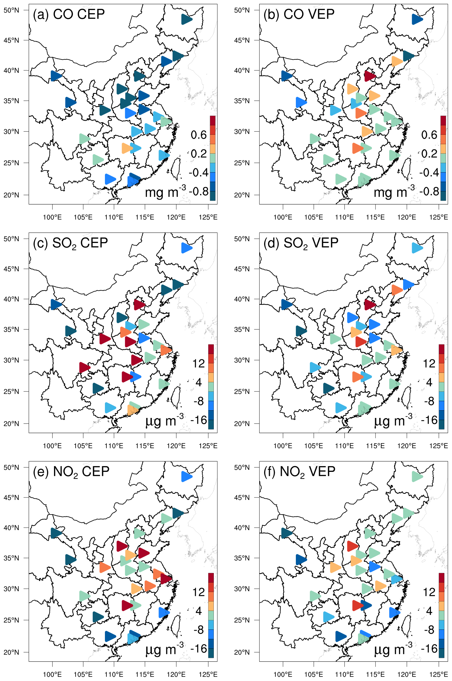
Figure 7 As in Fig. 5 but for the independent validation.

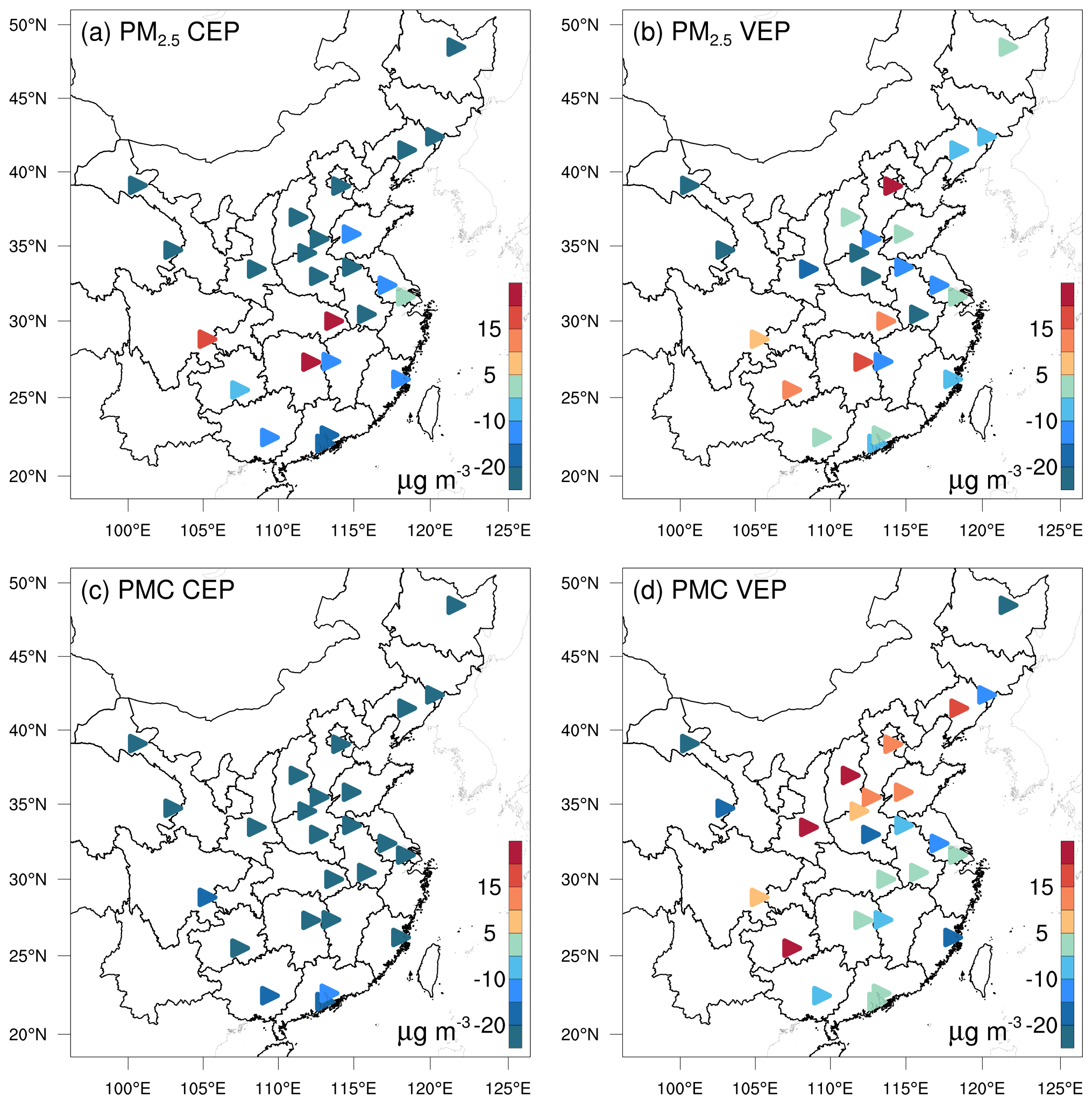
Figure 8 As in Fig. 6 but for the independent validation.

Comparing our results with those of previous studies, Tang et al. (2013) inverted CO emissions over Beijing and the surrounding areas and obtained comparable improvements (Table 6) in the RMSE (37 %–48 % vs. 30 %–51 %) and CORR (both studies ∼ 0.81); however, we decreased the biases by 90 %–97 %, which is much greater than their 48 %–64 % reductions. Additionally, Chen et al. (2019) showed that the RMSE of simulated SO₂ with updated SO₂ emissions decreased by 4.2 %–52.2 % for different regions, and the CORR only increased to 0.69 at most. These improvements are smaller than those obtained in this study, which may be due to the insufficient adjustment of emissions caused by the underestimated ensemble spread through the inflation method. The better performance in this study may be related to our inversion process, which causes the optimized emissions of the current DA window to propagate to the next DA window for further correction.

Table 6 Statistics comparing the pollution concentrations from the simulations with prior (CEP) and posterior (VEP) emissions against assimilated and independent observations, respectively. CO unit: mg m⁻³; other units: µg m⁻³. BIAS: mean bias; RMSE: root mean square error; CORR: correlation coefficient.

4.1.4 Uncertainty reduction

The uncertainty reduction rate (UR) is an important quantity to evaluate the performance of RAPAS and the effectiveness of in situ observations (Chevallier et al., 2007; Jiang et al., 2021; Takagi et al., 2011). Following Jiang et al. (2021), the UR was calculated as

$$\begin{array}{}\text{(19)}& \mathrm{UR}=\left(\mathrm{1}-{\displaystyle \frac{{\mathit{\sigma }}_{\mathrm{posterior}}}{{\mathit{\sigma }}_{\mathrm{prior}}}}\right)\times \mathrm{100},\end{array}$$

where σ_posterior and σ_prior are the posterior and prior uncertainties, respectively, calculated using the standard deviations of the prior and posterior perturbations. Figure 9 shows the URs averaged in each province and mainland China. URs varied with species as they are closely related to the magnitude settings of prior uncertainties (Jiang et al., 2021). The URs of PPM_2.5 and PMC were the most effective, while the UR of NO_x emissions was the lowest. For mainland China overall, uncertainties were reduced by 44.4 %, 45.0 %, 34.3 %, 51.8 %, and 56.1 % for CO, SO₂, NO_x, PPM_2.5, and PMC, respectively. For one species, URs varied across provinces. URs are usually related to observation coverage, which means that the more observation constraints there are, the more URs decrease. Additionally, URs may also be related to emission distributions. Generally, URs were more significant in the provinces where observations and emissions were both relatively concentrated (e.g., Tibet), while they were much lower where the emissions were scattered or relatively uniform, but the observations were only in large cities, even if there were many more observations in other provinces.

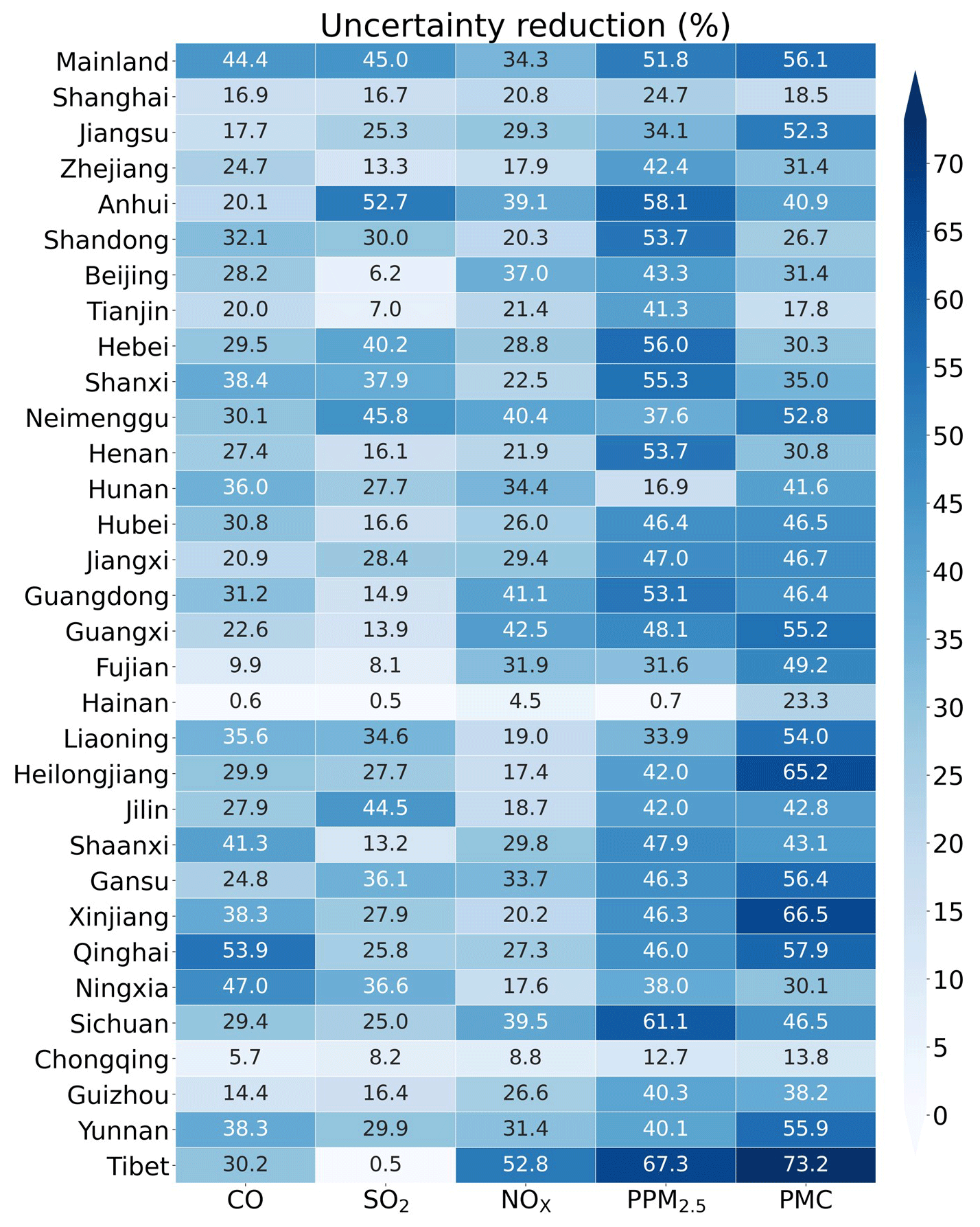
Figure 9 Time-averaged posterior emission uncertainty reduction (%) indicated by the standard deviation reduction in the total emissions per province calculated by prior and posterior ensembles.

4.1.5 Evaluation using chi-squared statistics

To diagnose the performance of the EnKF analysis, chi-squared (χ²) statistics were calculated, which are generally used to test whether the prior ensemble mean RMSE with respect to the observations is consistent with the prior “total spread” (square root of the sum of ensemble variance and observation error variance). Following Zhang et al. (2015), for the tth window, χ² is defined as

$$\begin{array}{}\text{(20)}& {\mathit{\chi }}_t^{\mathrm{2}}=(\mathit{y}-\mathbf{H}\stackrel{\mathrm{‾}}{{\mathbf{X}}^{\mathrm{b}}}{)}^{\mathrm{T}}({\mathbf{HP}}^{\mathrm{b}}{\mathbf{H}}^{\mathrm{T}}+\mathbf{R}{)}^{-\mathrm{1}}(\mathit{y}-\mathbf{H}\stackrel{\mathrm{‾}}{{\mathbf{X}}^{\mathrm{b}}}).\end{array}$$

Figure 10 shows the time series of the relative changes between the prior and posterior emissions and the χ² statistics. There were relatively large adjustments in emissions in the first three windows, especially for the PMC. Subsequently, the five species reached a more optimal state with successive emission inversion cycles. The χ² statistics showed similar variation characteristics to the daily changes in emissions. The χ² value was slightly greater than 1, indicating that the uncertainties from the error covariance statistics did not fully account for the error in the ensemble simulations. A similar result was reported by Chen et al. (2019). Further investigations should be conducted to generate larger spreads by accounting for the influence of model errors. As we imposed the same uncertainty in prior emissions at each DA window to partially compensate for the influence of model errors, χ² statistics showed small fluctuations, indicating that the system updated emissions consistently and stably.

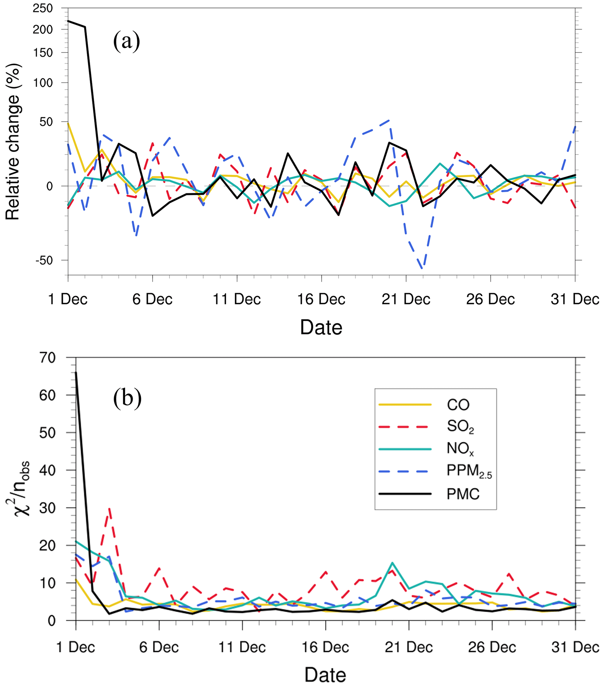
Figure 10 Relative changes (a) in posterior emission estimates of CO, SO₂, NO_x, PPM_2.5, and PMC and χ² statistics (b) of these state vectors in each window.

4.1.6 Evaluation using OSSE

Figure 11 shows the spatial distribution of the error reduction in the posterior emissions of the five species. After inversion, in most areas, the emission errors were reduced by more than 80 %, especially in the central and eastern regions with dense observation sites, while in remote areas far away from cities, due to the sparse observation sites, the emission errors were still not well adjusted. Overall, the error reduction rates of CO, SO₂, NO_x, PPM_2.5, and PMC were 78.4 %, 86.1 %, 78.8 %, 77.6 %, and 72.0 %, respectively, indicating that with the in situ observations in China, RAPAS can significantly reduce emission errors and thus showed good performance in emission estimates.

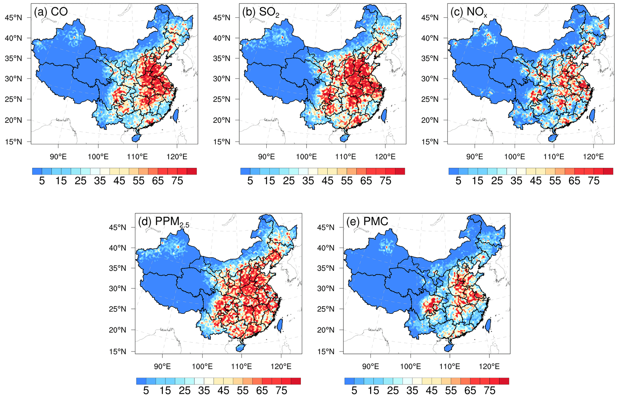
Figure 11 Spatial distribution of the error reduction (%) of posterior emissions in the OSSE.

4.2 Inverted emissions

Figure 12 shows the spatial distribution of temporally averaged prior and posterior emissions and their differences in emissions in December 2016. It should be noted that emissions outside China were masked; as the observation sites were limited to China in this study, there was a slight change in the emissions outside China. Higher emissions were mainly concentrated in central and eastern China, especially in the NCP, YRD, and Pearl River Delta, and lower emissions occurred across northwestern and southern China. Compared with the prior emissions, posterior CO emissions were considerably increased across most areas of mainland China, especially in northern China, with an overall increase of 129 %. A notable underestimation of prior emissions was also confirmed by inversion estimations (Feng et al., 2020b; Tang et al., 2013; Wu et al., 2020) and model evaluations (Kong et al., 2020) in previous studies. For SO₂, the emissions increased mainly in northeastern China, Shanxi, Ningxia, Gansu, Fujian, Jiangxi, and Yunnan provinces. In the SCB, central China, the YRD, and part of the NCP, emissions were significantly reduced. The national total SO₂ emissions increased by 20 %. For NO_x, although the increment of the national total emissions was small (approximately 5 %), there were large deviations. The emissions in the NCP and YRD were reduced, whereas the emissions in most cities in other regions increased. The changes in the emission of PPM_2.5 were similar to those of SO₂. Compared with the prior emissions, the posterior PPM_2.5 emissions decreased over central China, the SCB, and the YRD, whereas those in southern and northern China increased, especially in Shanxi, Shaanxi, Gansu, and southern Hebei provinces. Overall, the relative increase was 95 %. For PMC, the posterior emissions were increased over all of mainland China, with a national mean relative increase of 1045 %. Larger emission increments mainly occurred in areas with significant anthropogenic emissions of CO and PPM_2.5, indicating that the large underestimation of PMC emissions in the prior inventory may mainly be attributed to the underestimations of anthropogenic activities. The absence of natural dust is another reason, as the wind-blown dust scheme was not applied in this study. Overall, PM₁₀ emissions (PPM_2.5 + PMC) increased by 318 %. If we assume that all the increments in PM₁₀ emissions are from natural dust, it means the contribution of natural dust accounted for 75 % of total PM₁₀ emissions, which is consistent with the source apportionment of PM₁₀ of 75 % in Changsha in central China (Li et al., 2010). Large PMC emission increments were also reported by Ma et al. (2019).

Detailed estimations of posterior emissions and relative changes compared to prior emissions in each province and mainland China are given in Table S1. The evaluation results for July showed that the emission uncertainty could still be significantly reduced, and the performance of the system in July was comparable to that in December (Table S2). Additionally, the seasonal variation in emissions was well reflected (Figs. S4 and S5), which means that our system performed well at different times of the year. Note that the differences, excluding PMC, between the prior and posterior emissions mainly reflect the deficiencies of the prior emissions as the times of the prior emissions and observations were consistent in this study.

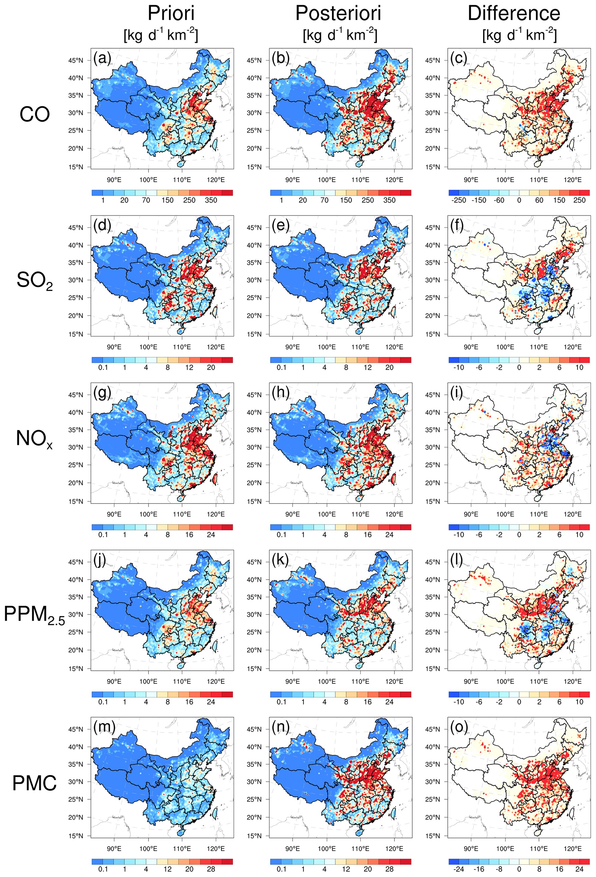
Figure 12 Spatial distribution of the time-averaged prior emissions (left column, MEIC 2016), posterior emissions (middle column), and differences (right column, posterior minus prior).

4.3 Sensitivity tests

4.3.1 Impact of prior inventories

Various prior inventories have shown considerable differences in space allocation and emission magnitudes. Inversion results can be sensitive to a priori emissions if the observations are insufficient (Gurney et al., 2004; He et al., 2018). MEIC 2012 was used as an alternative a priori in EMS1 to investigate the impact of different prior emissions on posterior emissions. Figure 13 shows the time series of the relative differences in the daily posterior emissions of the five species between the EMDA (base) and EMS1 experiments. Overall, the differences between the two posterior emissions gradually decreased over time. At the beginning, the differences in the CO, SO₂, NO_x, PPM_2.5, and PMC between the two inventories (i.e., MEIC 2012 vs. MEIC 2016) were 17.5 %, 114.5 %, 30.8 %, 46.0 %, and 72.0 %, respectively, compared to 2.5 %, 4.5 %, 4.5 %, −8.9 %, and 3.0 % in the last 10 d. In addition, the species with larger emission differences at the beginning took a longer time (i.e., more DA steps) to achieve convergence. The quick convergence of PMC emissions was attributed to the large prior uncertainty of 100 % used in the first three DA windows. In contrast to the other species, there were significant negative deviations in PPM_2.5 emissions between the two experiments. This may be due to the positive deviations in the precursors of PM_2.5 (i.e., SO₂ and NO_x), which lead to a larger amount of secondary production. The PPM_2.5 emissions will be reduced to balance the total PM_2.5. We compared the PM_2.5 concentrations simulated by the two optimized inventories and found that they were almost the same (Fig. S6). Overall, this indicates that observations in China were sufficient to infer emissions and that our system was robust. Meanwhile, the monthly posterior emissions shown in Sect. 4.2 were still underestimated to a certain extent.

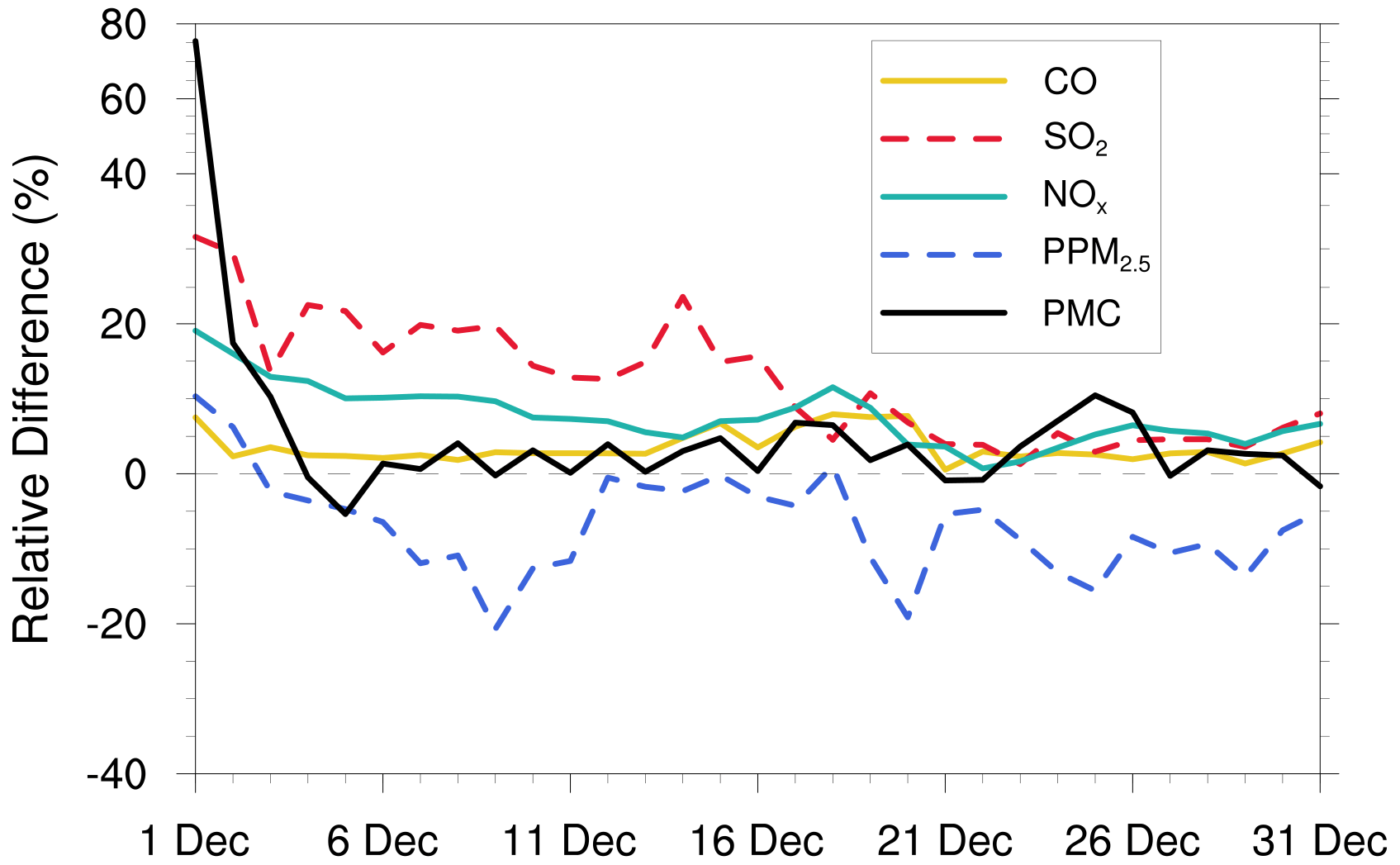
Figure 13 Relative differences in CO, SO₂, NO_x, PPM_2.5, and PMC emissions (%, the ratio of the absolute difference to EMDA) between the EMDA and EMS1 experiments.

4.3.2 Impact of prior uncertainty settings

The uncertainty of prior emissions determines how closely the analysis is weighted towards the background and observations; however, information about prior uncertainties is generally not readily available. To evaluate the possible influence of prior uncertainties on the optimized emissions, we increased and reduced the uncertainties after 3 d of cycling, starting at 00:00 UTC, 3 December, by 25 % and 50 % in EMS2 (−50 %), EMS3 (−25 %), EMS4 (+25 %), and EMS5 (+50 %), respectively. Table 7 summarizes the emission changes with different prior uncertainty settings in the EMS2–5 experiments. To better understand the response of the system to the emission uncertainty settings, Fig. 14 illustrates the time series of SO₂ emission changes, chi-squared statistics, and RMSEs of simulated SO₂ with emissions updated in the EMDA and EMS2–5 experiments over the YRD and NCP (Fig. 2). Compared with EMDA, when the uncertainties decreased (increased), the emissions of the five species decreased (increased) accordingly. This is because the posterior emissions of the five species were larger than the prior emissions, and, as shown in Fig. 14a–d, larger uncertainty will lead to faster convergence, resulting in larger posterior emissions. It can also be seen from Fig. 14 that a faster convergence will reduce the RMSE of the simulated concentration with the posterior emissions in the early stage of the experiment; however, in the later stage of the experiment, there were no significant differences in the RMSE and chi-squared statistics among the different experiments. However, day-to-day changes in emissions also cause slight fluctuations. In addition, when greater uncertainties are set, the day-to-day changes in emissions are more drastic, resulting in a larger RMSE, as shown in the NCP. Moreover, the significant day-to-day variations in the estimated emissions may not be in line with the actual situation. Owing to the spatial–temporal inhomogeneity of emissions, the differences in chi-squared statistics between the YRD and NCP show that it may be necessary to apply different a priori uncertainties according to different regions (Chen et al., 2019). Therefore, when using an EnKF system for emission estimation, error settings must be carefully executed. Overall, the uncertainties chosen in EMDA aim to minimize the deviation of the concentration fields and maintain the stability of the inversion.

Table 7 Relative differences in CO, SO₂, NO_x, PPM_2.5 and PMC emissions ( %, the ratio of the absolute difference to EMDA) between the EMDA and EMS2–5 experiments.

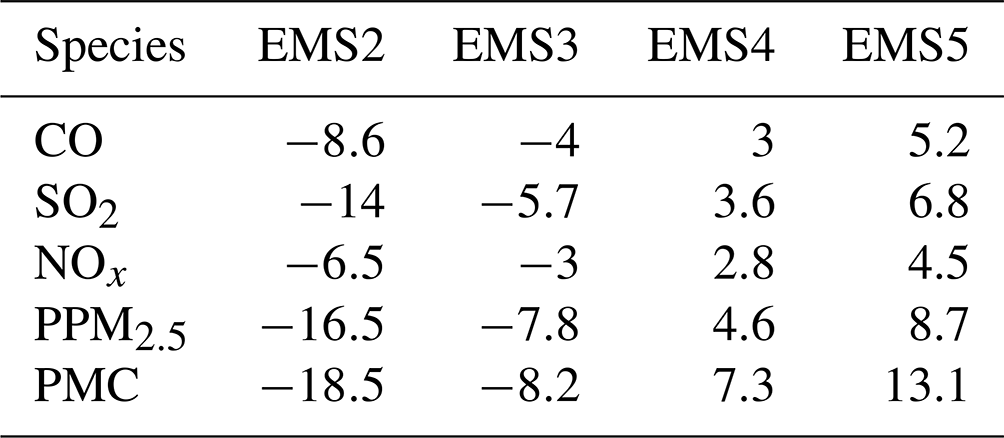
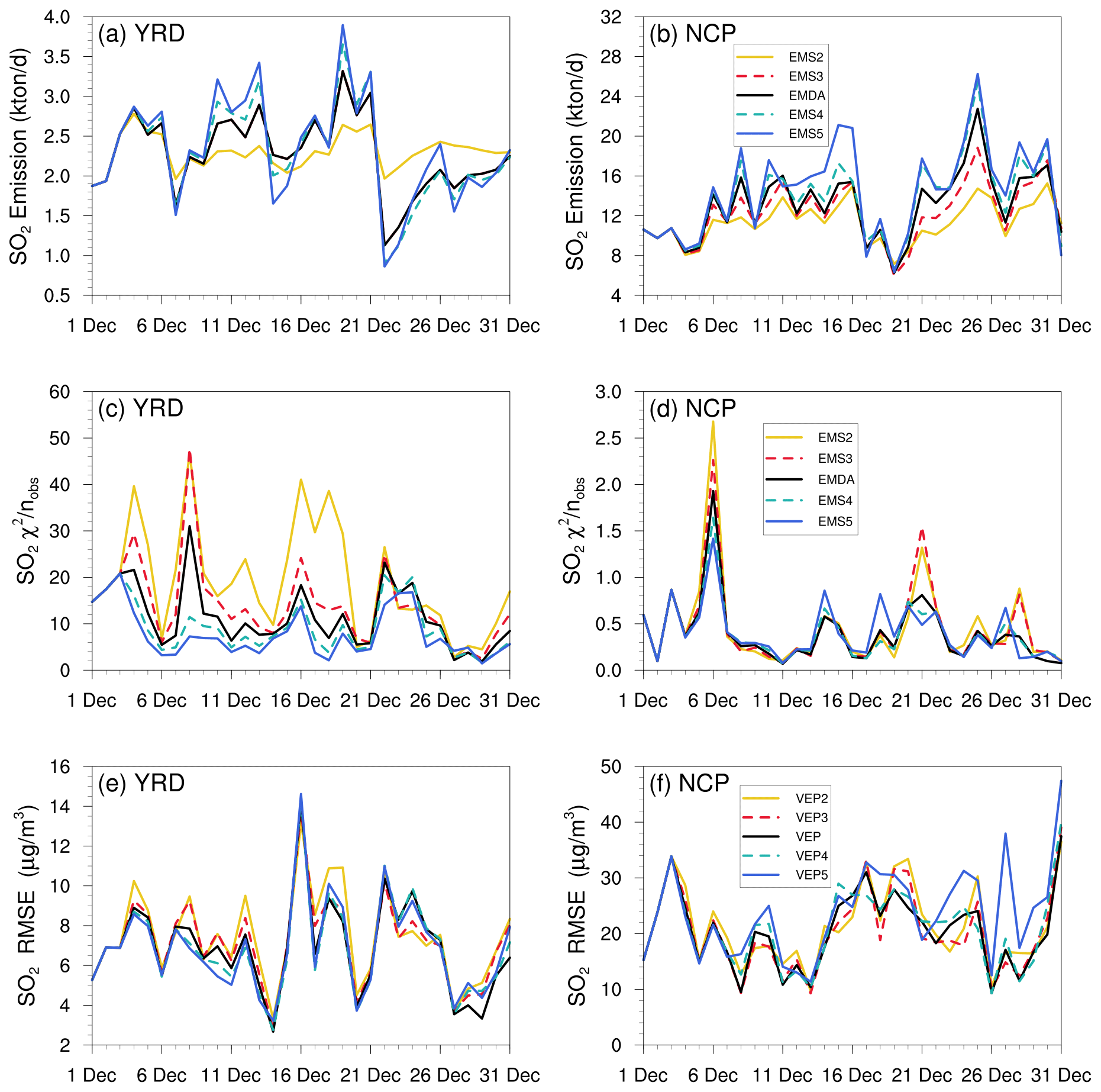
Figure 14 Time series of the SO₂ emission changes, chi-squared statistics, and RMSE of simulated SO₂ with updated SO₂ emissions in the EMDA and EMS2–5 experiments over the YRD and NCP.

4.3.3 Impact of observation error settings

Observation errors are another factor that determine the relative weights of the observations and background in the analysis. A proper estimate of the observation error is important for filter performance; however, observation errors are generally not provided with datasets. The observation error is usually set to a fixed value (Ma et al., 2019), specific proportion of the observation value (Tang et al., 2013), or value calculated by combining measurement error with representative error as used in this study. Generally, the performance of data assimilation is sensitive to the specification of the observation error (Tang et al., 2013). A sensitivity experiment (EMS6) with a doubled observation error was conducted to evaluate the influence of observation error on the optimized emissions. Overall, the spatial distribution of emissions after optimization was almost the same as that of the EMDA experiment but with a lower increment (Fig. S7), resulting in a weaker estimate of the national total emissions for each species. This is because the observation error inflates, and the system becomes more certain of the prior emission and reduces the effect of observation information. Figure 15 shows the time series of simulated and observed daily concentrations and their RMSEs verified against the assimilated sites. The simulations in VEP6 usually performed worse, with larger biases and RMSEs than those of VEP (Figs. S8 and S9), especially in western and southern China, where posterior emissions were significantly underestimated. These results generally corresponded to sluggish emission changes and large chi-squared statistics (Fig. S10), suggesting that an observation error that is too large may substantially impact the estimated emissions.

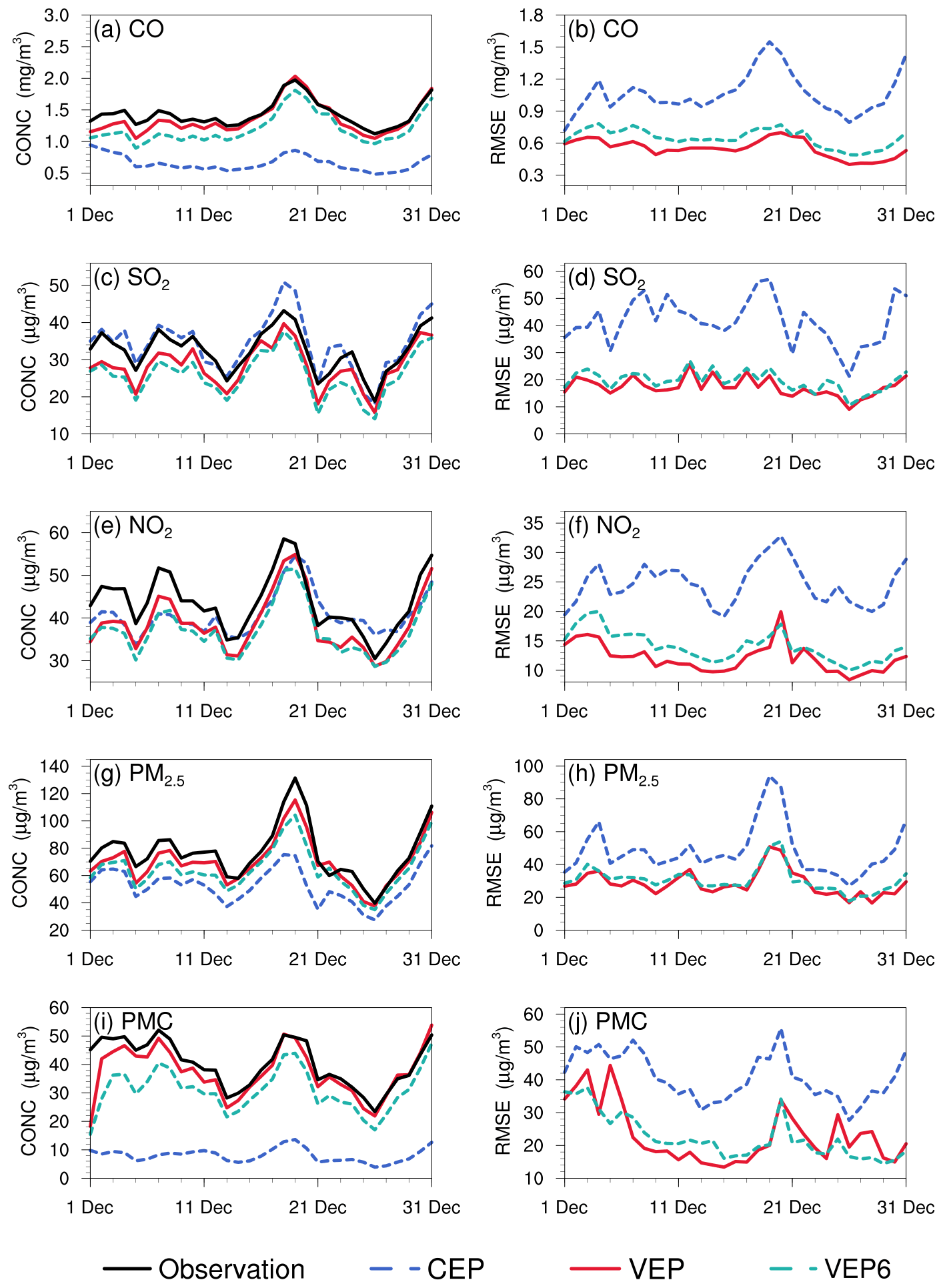
Figure 15 Time series of the daily concentrations (CONC, left) and root mean square error (RMSE, right) obtained from CEP, VEP, and VEP6. The simulations were verified against the assimilated sites.

4.3.4 Impact of the IC optimization of the first window

Several studies indicate large emission discrepancies resulting from IC errors (Jiang et al., 2013a; Miyazaki et al., 2017; Tang et al., 2013), which means that if the IC is not optimized, the errors in concentrations would be compensated for through the adjustment of emissions. To evaluate the impact of IC optimization of the first window on the emission inversions, an EMS7 experiment without the IA step was conducted. Figure 16 shows the time series of the relative differences in the daily posterior emissions of the five species between the EMDA and EMS7 experiments. It can be observed that IC optimization had a significant impact on the emission inversions of long-lived species (i.e., CO). The overall difference in the inverted CO emissions between the two experiments was approximately 5.3 % but can reach 26.1 % in the first few windows. For the short-lived species, IC optimization had little impact on the emissions; for example, the average emission differences of SO₂, NO_x, and PMC in the two experiments were 0.3 %, 0.3 %, and 0.9 %, respectively. For PPM_2.5, the average emission difference is affected not only by primary emissions, but also by the complex chemistry of its precursors. Therefore, the difference between the two experiments fluctuated, with an overall difference of 2 %. Notably, with the gradual disappearance of the benefit of IC assimilation, the two experiments reached a unified state after several windows. For CO, the impact of IA on emission inversion lasted approximately half a month. These results indicate that removing the bias of the IC of the first DA window is essential for the subsequent inverse analysis (Jiang et al., 2017).

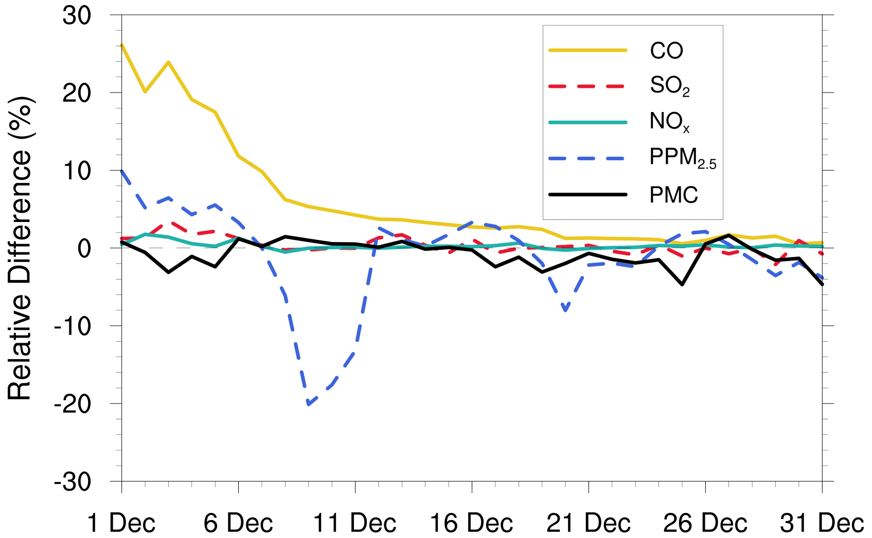
Figure 16 Relative differences in CO, SO₂, NO_x, PPM_2.5, and PMC emissions (%, the ratio of the absolute difference to EMDA) between the EMDA and EMS7 experiments.

4.4 Discussion

Optimal state estimation using an EnKF relies on the assumption of an unbiased Gaussian prior error, which is not guaranteed in such highly nonlinear and large-bias systems. In this study, some pollutants (e.g., CO, PMC) have very large simulated biases; thus, if a small uncertainty is adopted, the emission bias cannot be fully reduced. If a very large uncertainty is adopted, then the degree of freedom of adjustment is too large, and the inverted daily emissions will fluctuate abnormally. Therefore, we only set a larger prior uncertainty in the first three windows, adopting a moderate uncertainty in the following windows, and used a two-step inversion scheme and cyclic iteration to gradually correct the emission errors. Figure 10a shows the time series of the relative differences between prior and posterior emissions in each window. There were relatively large adjustments for the emissions in the first three windows, especially for PMC, but the adjustment ranges of the five species after the first three windows were within the uncertainty range (e.g., ±25 %), indicating that with this scheme, the EnKF method used in this system performed well in emission inversion.

Model–data mismatch errors are from both the emissions and the inherent model errors arising from the model structure, discretization, parameterizations, and biases in the simulated meteorological fields. Neglecting model errors would attribute all uncertainties to emissions and lead to considerable bias in the estimated emissions. In the version of the CMAQ model used in this study, there are no heterogeneous reactions (Quan et al., 2015; Wang et al., 2017), the parameterization scheme for the formation of secondary organic aerosols (SOAs) is imperfect (Carlton et al., 2008; Jiang et al., 2012a; Yang et al., 2019), no feedback between chemistry and meteorology was considered, and we used an idea profile for chemical lateral boundary conditions. All the above problems can lead to underestimated concentrations of pollutants, which in turn require more emissions to compensate for this, leading to overestimation of emissions. In addition, previous studies have shown that ammonia emissions in the MEIC inventory are underestimated (Kong et al., 2019; Paulot et al., 2014; Zhang et al., 2018). Owing to the lack of ammonia observations, our system does not include emission estimates of ammonia, which means that the concentration of ammonium aerosol was underestimated in this system, also resulting in an overestimation of the PPM_2.5 emission. Wind-blown dust was also not simulated; thus, the PMC emission inverted in this system comes from anthropogenic activities and natural sources. Although some of these shortcomings can be solved by updating the CTM model, there will still be errors in each parameterization and process. In general, a parameter estimation method was used to reduce the model errors, in which some uncertain parameters were included in the augmented state vector and optimized synchronously based on the available observations (Brandhorst et al., 2017; Evensen, 2009). However, it is difficult to identify the key uncertain parameters of different species in different models, which generally comes not only from the complex atmospheric chemical model but also from hundreds of model inputs (Tang et al., 2013). Another method is bias correction, which treats the model error as a bias term and includes it in an augmented state vector (Brandhorst et al., 2017; De Lannoy et al., 2007; Keppenne et al., 2005). In addition, the weak-constraint 4D-Var method can be used to reduce model errors, which adds a correction term in the model integration to account for the different sources of model error (Sasaki, 1970). Although the reliable diagnosis of model error remains a challenge (Laloyaux et al., 2020), it should be considered in an assimilation system. In the future, we will consider model errors in our system to obtain better emission estimates.

Independent variable localization was adopted to avoid potential spurious correlations across different species in this study. However, the transmission scales for different species in different regions differ, and a more accurate localization range can be obtained through backward trajectory analysis. In addition, O₃ observations were not assimilated to improve NO_x and VOC emissions using cross-species information. O₃ concentrations and NO_x (VOC) emissions were positively correlated in the NO_x (VOC)-limited region and negatively correlated in the VOC (NO_x)-limited region (Tang et al., 2011; N. Wang et al., 2019). Hamer et al. (2015) successfully used O₃ observations to estimate NO_x and VOC emissions within the 4D-Var framework within an ideal model. However, the NO_x emissions are often point or line sources, which are all small compared to the model resolution. With a coarse spatial resolution, the model cannot accurately simulate the relationships between O₃ and its precursors. When assimilating O₃ observations to infer NO_x or VOC emissions, the inaccurate relationships simulated by the model would worsen the inversion of NO_x emissions (Inness et al., 2015). In general, improving the model resolution can improve the detailed simulation and provide better prior information on O₃–NO_x–VOC, but it is still difficult to determine whether the condition is NO_x-limited or VOC-limited in the real atmosphere using prior emissions (Liu and Shi, 2021). Elbern et al. (2007) emphasized that assimilating O₃ to correct NO_x or VOC emissions must follow the EKMA framework derived based on observations, otherwise, even if the resolution is improved to sufficiently solve point and line sources, precursor emissions may still be adjusted in an opposite direction. This can be demonstrated in our OSSE experiment at a high resolution of 3 km (Fig. S11). In this study, the spatial resolutions of the prior emission inventory (i.e., MEIC) is 0.25^∘ × 0.25^∘, which is appropriate for modeling at regional scales (Zheng et al., 2017). With this emission inventory, it is unable to accurately simulate the O₃–NO_x–VOC relationships. Therefore, to avoid the impact of inaccurate O₃–NO_x relationships on emission inversion, in our system, we did not assimilate O₃ but directly assimilated NO₂ to optimize the NO_x emissions. This work will be followed by an ongoing study using the available VOC observations.

Although we do not assimilate O₃ observations, model resolution still has some influence on inversion results. In our previous study (Feng et al., 2022), we inferred the NO_x emissions over the YRD in China using NO₂ observations, which has a spatial resolution of 12 km. The study period, assimilated observations, and inversion settings are the same as in this study. We compared the posterior emissions of the YRD between this study and Feng et al. (2022). The results showed that there was a similar spatial distribution of posterior emissions inferred using the two resolutions (36 km vs. 12 km) (Fig. S12), but the total NO_x emission in the YRD inferred using the 36 km resolution was about 8.8 % higher than that inferred using the 12 km resolution. The differences are mainly caused by meteorological differences at different resolutions. This indicates that coarse model resolution may lead to some overestimation of the inverted emissions. In addition, as shown previously, the concentrations after DA were evidently underestimated in western China, indicating that the inverted emissions over these regions still have large uncertainties because of the sparsity of observations, which are spatially insufficient for sampling the inhomogeneity in emissions. Therefore, further investigations with the joint assimilation of multi-source observations (e.g., satellite) are underway.

NO_x is mainly emitted by transportation (Li et al., 2017), which can reflect the level of economic activity to a certain extent. Weekly emission changes were explored to verify the performance of the system in depicting emission changes (Fig. S13). Although the “weekend effect” of emissions in China is not significant (Wang et al., 2014, 2015), the posterior NO_x emission changes are in good agreement with the observations. In our previous studies (Feng et al., 2020a, b), this system was successfully applied to optimize NO_x and CO emissions. The inverted emission changes were also in line with the epidemic control time points. Additionally, the emission changes can reflect the emission migration from developed or urban areas to developing or surrounding areas in recent years, which is consistent with the emission control strategies in China. Although the system did not consider the model error, resulting in a certain difference between the posterior and actual emissions, the spatiotemporal changes in posterior emissions were relatively reasonable and can be used to monitor emission changes and inform emission regulations.

5 Summary and conclusions

In this study, we developed a Regional multi-Air Pollutant Assimilation System (RAPAS v1.0) based on the WRF–CMAQ model, 3D-Var algorithm, and EnKF algorithm. RAPAS can quantitatively optimize gridded emissions of CO, SO₂, NO_x, PPM_2.5, and PMC on a regional scale by simultaneously assimilating hourly in situ measurements of CO, SO₂, NO₂, PM_2.5, and PM₁₀. This system includes two subsystems: the IA subsystem and the EI subsystem, which optimize chemical ICs and infer anthropogenic emissions.

Taking the 2016 MEIC in December as a priori, the emissions of CO, SO₂, NO_x, PPM_2.5, and PMC in December 2016 were inferred by assimilating the corresponding nationwide observations over China. The optimized ICs and posterior emissions were examined against assimilated and independent observations through parallel forward-simulation experiments with and without DA. Sensitivity tests were performed to investigate the impact of different inversion processes, prior emissions, prior uncertainties, and observation errors on emission estimates.

RAPAS showed a good performance in assimilating surface in situ observations, with the calculated emission uncertainties reduced by 44.4 %, 45.0 %, 34.3 %, 51.8 %, and 56.1 % for CO, SO₂, NO_x, PPM_2.5, and PMC, respectively. It can also significantly improve the simulations; the RMSEs of the simulated concentrations with posterior emissions decreased by 40.1 %–56.3 %, and the CORRs increased from 0.26–0.66 to 0.69–0.87 for different species. The OSSE experiment showed that the errors of posterior CO, SO₂, NO_x, PPM_2.5, and PMC could be reduced by 78.4 %, 86.1 %, 78.8 %, 77.6 %, and 72.0 %, respectively. Overall, compared with the prior emissions (MEIC 2016), the posterior emissions increased by 129 %, 20 %, 5 %, and 95 % for CO, SO₂, NO_x, and PPM_2.5, respectively. The posterior PMC emissions, which included anthropogenic and natural dust contributions, increased by 1045 %. Sensitivity tests with different prior inventories showed that the observations in China were sufficient to infer emission and that our system was less dependent on prior inventories. Additionally, sensitivity tests with different prior uncertainties indicated that when the posterior emissions were larger than the prior emissions, the emissions decreased (increased) with decreases (increases) in uncertainties because of the different convergence rates. These results demonstrate the advantage of the two-step method in emission inversion in that the inversion errors of the last window can be transferred to the current window for further optimization, thus enhancing the robustness of emissions estimation using nationwide observations over China with RAPAS. It should be noted that the system usually responds slowly to too small a priori uncertainties or too large observation errors, which may result in large errors in the estimated emissions.

In summary, the comprehensive evaluation and sensitivity tests revealed that RAPAS could serve as a useful tool for accurately quantifying the spatial and temporal changes in multi-species emissions at regional scales and in near-real time, which will be helpful for air pollution control in China and other regions around the world with dense ground observation networks.