Key factors for quantitative precipitation nowcasting using ground weather radar data based on deep learning

Quantitative precipitation nowcasting (QPN) can help to reduce the enormous socioeconomic damage caused by extreme weather. The QPN has been a challenging topic due to rapid atmospheric variability. Recent QPN studies have proposed data-driven models using deep learning (DL) and ground weather radar. Previous studies have primarily focused on developing DL models, but other factors for DL-QPN have not been thoroughly investigated. This study examined four critical factors in DL-QPN, focusing on their impact on forecasting performance. These factors are the deep learning model (U-Net, as well as a convolutional long short-term memory, or ConvLSTM), input past sequence length (1, 2, or 3 h), loss function (mean squared error, MSE, or balanced MSE, BMSE), and ensemble aggregation. A total of 24 schemes were designed to measure the effects of each factor using weather radar data from South Korea with a maximum lead time of 2 h. A long-term evaluation was conducted for the summers of 2020–2022 from an operational perspective, and a heavy rainfall event was analyzed to examine an extreme case. In both evaluations, U-Net outperformed ConvLSTM in overall accuracy metrics. For the critical success index (CSI), MSE loss yielded better results for both models in the weak intensity range (≤ 5 mm h⁻¹), whereas BMSE loss was more effective for heavier precipitation. There was a small trend where a longer input time (3 h) gave better results in terms of MSE and BMSE, but this effect was less significant than other factors. The ensemble by averaging results of using MSE and BMSE losses provided balanced performance across all aspects, suggesting a potential strategy to improve skill scores when implemented with optimal weights for each member. All DL-QPN schemes exhibited problems with underestimation and overestimation when trained by MSE and BMSE losses, respectively. All DL models produced blurry results as the lead time increased, while the non-DL model retained detail in prediction. With a comprehensive comparison of these crucial factors, this study offers a modeling strategy for future DL-QPN work using weather radar data.

1 Introduction

Short-term precipitation forecasting is an essential topic in weather forecasting, providing crucial information related to socioeconomic effects in daily life. Short-term precipitation forecasting within 2 h is generally called quantitative precipitation nowcasting (QPN), which can be of great assistance in preventing damage from severe precipitation over a short period (Prudden et al., 2020). Despite the critical importance of QPN, it has been a challenging issue for a long time because of the complexity and dynamic characteristics of the atmosphere (Ravuri et al., 2021). Two major approaches to QPN exist: numerical weather prediction (NWP) and statistical extrapolation (Prudden et al., 2020). NWP simulates future atmospheric conditions, such as precipitation, pressure, temperature, and wind vectors, based on physical governing equations and global data assimilation. Even though NWP has been improved over decades with higher prediction skills and denser spatiotemporal resolution, NWP for QPN still has limitations due to its high computational cost, synoptic-scale prediction, and spin-up issues (Yano et al., 2018; Bowler et al., 2006). For short-term forecasting of precipitation, QPN has generally adopted extrapolation of the sequence of weather radar to focus on local rainfall with relatively high estimation accuracy (Wang et al., 2009; Ravuri et al., 2021; Prudden et al., 2020; Ayzel et al., 2020). Generally, QPN extrapolates the precipitation pattern using only radar sequences (Shi et al., 2015; Ravuri et al., 2021), but it can integrate other data sources, such as weather stations, NWP, and satellite data (Bowler et al., 2006; Haiden et al., 2011; Chung and Yao, 2020).

Weather radar provides real-time distribution of precipitation with high spatial (approximately 0.5–1 km) and temporal (about 5–10 min) resolutions. Various extrapolation approaches have been used for QPN from time series weather radar data. Temporal extrapolation of the radar sequence demonstrated high prediction accuracy for 1–2 h lead times, but the performance degraded as lead times increased. Several radar extrapolation methods have been developed, including thunderstorm identification tracking analysis and nowcasting (TITAN), tracking radar echo by correlation (TREC), and the McGill Algorithm for Precipitation Nowcasting by Lagrangian Extrapolation (MAPLE) (Dixon and Wiener, 1993; Mecklenburg et al., 2000; Germann and Zawadzki, 2002; Turner et al., 2004; Germann and Zawadzki, 2004). Despite their superior performance within a few hours compared with NWP, there have been limitations in predicting the onset of precipitation (Kim et al., 2021).

Recent advances in deep learning (DL) have altered conventional weather forecasting methods, especially for short-term predictions like QPN. The radar-based QPN can be viewed as a spatiotemporal video prediction that simulates upcoming frames based on past sequences (Han et al., 2023). Some studies used multiple input sources, such as meteorological variables, ground measurements, and NWP data (Adewoyin et al., 2021; Chen and Wang, 2022; F. Zhang et al., 2021; Kim et al., 2021), but the majority of studies used only radar precipitation without any additional input sources. Among DL approaches, convolutional neural networks (CNNs) are widely used for spatial modeling in computer vision and geoscientific fields. Recurrent neural networks (RNNs) are expected to perform well on time series datasets owing to their architecture, which recursively feeds the output as the following input and handles successive sequence data. Basic RNNs are not designed to consider spatial information, so there have been attempts to use RNNs for precipitation forecasting for each gauge station (Kang et al., 2020). Shi et al. (2015) suggested convolutional long-short term memory (ConvLSTM) to combine the benefits of CNN and RNN to improve QPN performance in Hong Kong. ConvLSTM was designed to model spatiotemporal prediction by applying long short-term memory (LSTM), one of the most popular RNN models, to convolutional CNN operations. Other RNN-based models of the trajectory gated recurrent unit (TrajGRU) and convolutional gated recurrent unit (ConvGRU) were proposed by (Shi et al., 2017). They reported that the deep learning models outperformed the operational models based on real-time optical flow by variational methods for echoes of radar (ROVER) by the Hong Kong observatory. Several studies using ConvLSTM, TrajGRU, and ConvGRU have demonstrated the superiority of CNN and RNN models over traditional approaches (Franch et al., 2020; Chen et al., 2020; Y. Zhang et al., 2021; Ravuri et al., 2021). However, some studies have only used CNNs for DL-QPN. The most widely used model is the U-Net (Ronneberger et al., 2015), which has a U-shaped structure with cascaded encoders, decoders, and skip connections. As U-Net can predict upcoming radar precipitation frames with a more straightforward form than RNN-fused models, it has been widely adopted in recent QPN studies employing deep learning (Ayzel et al., 2020; Agrawal et al., 2019; Samsi et al., 2019; Ko et al., 2022; Kim and Hong, 2021). In several application domains, CNNs have demonstrated their numerical robustness during training and made more accurate predictions than RNNs (Bai et al., 2018; Gehring et al., 2017). Recent studies have indicated that deep learning has become the predominant method for QPN owing to its superior performance compared to traditional approaches. However, there is still a dearth of exploration of the various considerations for the DL-QPN besides the DL model itself. As most studies have primarily focused on developing DL models across multiple study areas and datasets, it is difficult to determine how other factors can affect the skill score, even if they are crucial.

Considering this context, this study investigates critical factors that affect a DL-QPN model. Categorizing key factors in the DL-QPN is challenging, as there is a lack of standard agreement or explicit considerations in the literature. After analyzing various experimental designs used in previous studies, we summarized the following four critical factors in the DL-QPN: (1) the DL model, (2) the input sequence length, (3) the loss function, and (4) ensemble aggregation. The DL model has been the most highlighted factor in previous DL-QPN studies. The two representative types are fully convolutional networks (FCNs) and a combination of CNN and RNN. U-Net (Agrawal et al., 2019; Ayzel et al., 2020; Trebing et al., 2021; Kim and Hong, 2021) and ConvLSTM (Shi et al., 2015; Jeong et al., 2021; Xiong et al., 2021) are the most popular models for FCN and CNN-RNN in DL-QPN, respectively. As the DL-QPN is data-driven, the sequence length will likely determine the model performance. However, the data sequence length has rarely been investigated in previous studies. Various time steps from 25 to 180 min were used as input data to predict future radar precipitation for up to 360 min, with little explicit comparison in the literature. Hence, the input sequence lengths were included as critical factors for further in-depth analysis. The loss function is a crucial element as it guides the training process of the model. In this context, we examined two widely employed loss functions in DL-QPN: the mean squared error (MSE) and the balanced MSE (BMSE). Lastly, we viewed ensemble of schemes as a potential key factor in DL-QPN. Although the ensemble method has not yet been a major topic of discussion in DL-QPN, we believe that this approach holds significant potential for enhancing accurate nowcasting in the future. A detailed explanation of these four key factors is provided in Sect. 2.

In this study, we compared diverse DL-QPN schemes considering four factors along with a non-DL model. Experiments were conducted in South Korea using weather radar data from 2012–2022 over June to August. As the DL-QPN is highly anticipated to mitigate damage from severe weather, heavy rainfall events in the Korean Peninsula were examined in detail. The remainder of this paper is organized as follows. A detailed explanation of the four key factors and comparison schemes is provided in Sect. 2. Section 3 describes the data and methods used. Section 4 presents the results, and Sect. 5 discusses the results. Finally, Sect. 6 concludes the paper.

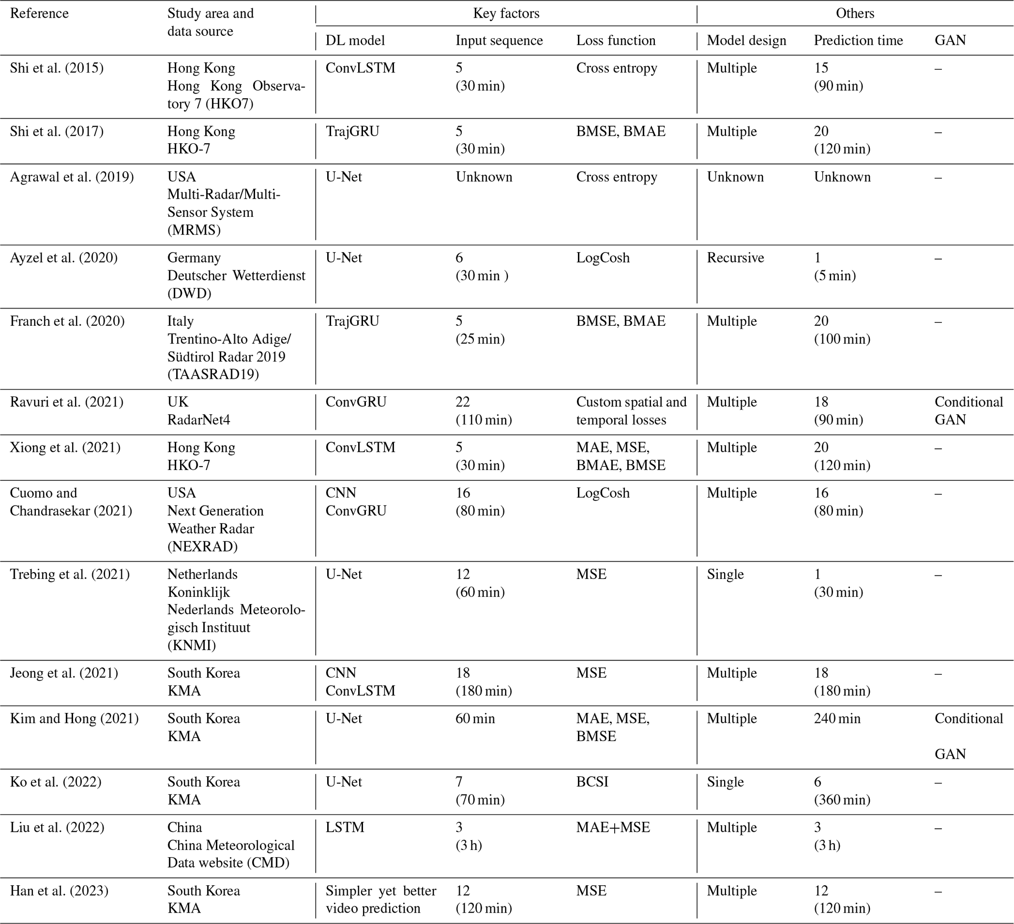
Table 1 Summary of key factors used in previous image-to-image QPN only using radar sequence based on deep learning. “B” in the loss column stands for “balanced,” which blends different weights for rainfall intensity or each input time.

2 Key factors in DL-QPN

2.1 Deep learning model

The four critical factors identified from previous DL-QPN studies using weather radar are summarized in Table 1. Two basic models are CNN and RNN. CNNs have been widely adopted in various DL-QPN studies because of their outstanding performance in spatial modeling in various remote sensing and environmental studies including atmosphere (Lee et al., 2021; Gardoll and Boucher, 2022; Geiss et al., 2022; Chattopadhyay et al., 2022; Kim et al., 2018), ocean (Chinita et al., 2023; Barth et al., 2022; Kim et al., 2023), urban and land (Wu et al., 2022; Sato and Ise, 2022; Qichi et al., 2023), and cryosphere (Lu et al., 2022; Y. J. Kim et al., 2020; Chi and Kim, 2021). The crucial part of CNNs is finding optimal convolutional filters to predict the target value with input data. The set of convolutional filters with specific window sizes (e.g., 3 × 3 or 5 × 5) was initialized with dummy values. The initial prediction is generated by conducting the dot product between the filters and the input over the cascading layers. The total error is calculated using the loss function between the model prediction and the actual value. The L1 (mean absolute error, MAE) or L2 (mean squared error, MSE) loss function is commonly used in supervised learning for regression; however, other types of loss functions can be used in DL-QPN (Ayzel et al., 2020; Ravuri et al., 2021). Following the loss calculation, the weights of the convolutional layers are updated through backpropagation. With an increasing number of iterations, the model was progressively fitted to the given dataset.

U-Net is one of the most representative image-to-image models among CNNs. Because DL-QPN can be viewed as image-to-image modeling, U-Net has been widely adopted in recent DL-QPN studies (Ayzel et al., 2020; Bouget et al., 2021; Ko et al., 2022; Kim and Hong, 2021). U-Net consists solely of convolutional layers that can preserve spatial information from the input to the output. The input for the DL-QPN with weather radar is the previous sequence of the radar images. This model is expected to generate a series of future precipitation scenes. The input and output are image sequences with the dimensions of [$ny,nx,M$] and [$ny,nx,N$], where M and N are the lengths of the sequence in the past and future, respectively. Its skip connections distinguish U-Net between the same level of encoding and decoding layers, which can mitigate the loss of original information as the network deepens (Ronneberger et al., 2015). In this study, RainNet v1.0 (https://github.com/hydrogo/rainnet, last access: 16 October 2023) by Ayzel et al. (2020) was adopted for the U-Net model.

RNNs are expected to yield good performance in time series forecasting. An RNN is distinguished by its recurrent layers, which feed the output of a specific layer back to its input. As the vanilla RNN structure suffers from the vanishing gradient problem with an increasing number of recurrent hidden layers, revised RNNs, such as long short term memory (LSTM) and gated recurrent units (GRU), have gained widespread acceptance (Cho et al., 2014; Hochreiter and Schmidhuber, 1997). They added additional gates to control the information transmitted or dropped, resulting in improved performance compared with vanilla RNNs. Several studies have been conducted on using RNNs for short-term rainfall forecasting (Ni et al., 2020; Aswin et al., 2018). However, these were station-based rainfall predictions that did not account for 2-D information because RNNs were not designed to take spatial information into account. Shi et al. (2015) suggested the ConvLSTM, which combines CNN and LSTM into a single model. Because ConvLSTM has been adopted in recent DL-QPN studies (Chen et al., 2020), it was compared with U-Net in this study. A detailed explanation of the ConvLSTM can be found in Shi et al. (2015).

2.2 Input sequence length

The DL-QPN predicts upcoming precipitation based on past sequences. Thus, the composition of the past series directly affects the model performance. A longer past sequence may provide more information than a shorter one, but it could also contain redundant information for model training. The optimal length of the past sequence can vary depending on other factors, such as the forecasting design, DL model, radar time interval, and maximum lead time. Thus, it is difficult to determine the direct effect of past sequence length on DL-QPN. To examine the impact of the input sequence length, we compared radar sequences of 1, 2, and 3 h against 12 future radar scenes for 2 h. This sets up a ratio of input–output sequences at 1:2, 1:1, and 3:2.

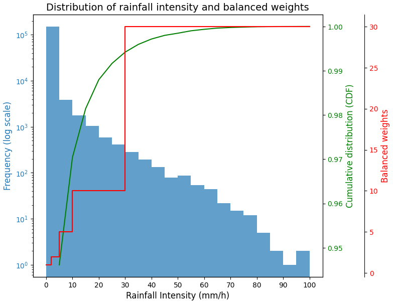
Figure 1 Mean distribution of rainfall intensity for the summers of 2020–2022 in a pixel window of 400 × 400. The blue bar represents the histogram of rainfall intensity. The green line shows the cumulative distribution function. The red line represents the balanced weights for mitigating data imbalances, as suggested by Shi et al. (2017).

2.3 Balanced loss function

The loss function guides the direct optimization of DL models. The basic loss function in DL-QPN is MSE (Eq. 1). By summing up the error of each pixel, it produces a single value for a given prediction image. As most valid precipitation pixels are severely skewed in weak rainfall intensity approximately ≤ 5 mm h⁻¹ (Fig. 1), calculating MSE with a uniform weight for all pixels might result in an underestimation problem across the range of values. Shi et al. (2017) suggested the BMSE to mitigate the sample imbalance by using different weights for precipitation intensity (Eq. 2).

$$\begin{array}{}\text{(1)}& \mathrm{MSE}={\displaystyle \frac{\sum _{i=\mathrm{1}}^N{\left(y_i-{\widehat{y}}_i\right)}^{\mathrm{2}}}{N}},\end{array}$$

$$\begin{array}{}\text{(2)}& \begin{array}{rl}\mathrm{BMSE}=& {\displaystyle \frac{\sum _{i=\mathrm{1}}^{N}w\left(y_i\right){\left(y_i-{\widehat{y}}_i\right)}^{\mathrm{2}}}{N}},\\ w\left(y_i\right)=& \left\{\begin{array}{l}\mathrm{1},y_i<\mathrm{2}\\ \mathrm{2},\mathrm{2}<y_i<\mathrm{5}\\ \mathrm{5},\mathrm{5}<y_i<\mathrm{10}\\ \mathrm{10},\mathrm{10}<y_i<\mathrm{30}\\ \mathrm{30},y_i>\mathrm{30}\end{array}\right.,\end{array}\end{array}$$

where y is the reference value, $\widehat{y}$ represents the predicted value, and N is the number of all valid pixels within the radar area. Figure 1 shows the distribution of rainfall intensity and weights for BMSE.

2.4 Ensemble approach

Ensemble approaches have been adopted as the standard in NWP by combining multiple different members to produce robust results. Despite their potential, ensemble approaches have not been actively adopted in DL-QPN. The ensembling of multiple schemes can bring enhanced and more stable performance than a single model in various evaluation aspects. An ensemble approach can be executed with simple aggregation with equal weights, or it can employ another machine learning model to learn the optimal way of combining each prediction, such as a stacking ensemble (Cho et al., 2020; Franch et al., 2020). The primary interest of this study is how the results can be improved through ensemble approaches. Hence, only a simple ensemble was done by averaging results from multiple schemes with same weight.

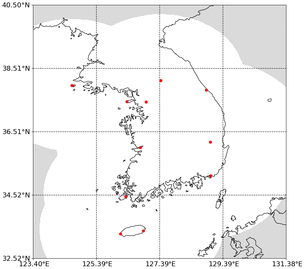
Figure 2 Weather radar over the Korean Peninsula used in this study. The grey shadow at the boundary indicates the area outside of valid radar coverage. The locations of the 11 weather radars are represented by red dots.

3 Data and methods

3.1 Data and preprocessing

South Korea, located in northeastern Asia, has a population of approximately 50 million and hosts numerous industrial facilities. Every year, particularly during the summer monsoon season, the country experiences flooding, inundation, and landslides. Sudden heavy rainfall can occasionally disrupt urban transportation systems, and continuous heavy rain during the rainy season (Jangma in Korean) can result in dam failures and significant flooding in river basins. A total of 11 ground weather radars have been operated by the Korea Meteorological Administration (KMA) to monitor precipitation over South Korea. Multiple radars were combined to produce a composite radar reflectance image with a spatial resolution of 1 km (Fig. 2). We used the constant altitude plan position indicator (CAPPI), widely used to study precipitation, with an altitude of 1.5 km provided by the KMA (Shi et al., 2017; Han et al., 2019; Kim et al., 2021). To exclude the area outside the radar coverage, we cropped the data from 33 to 39^∘ N and 124 to 131.15^∘ E. This encompasses most of the national territory of South Korea and a portion of North Korea. For the long-term test, the CAPPI dataset was collected every 10 min from 2012 to 2022 during the months of June, July, and August (JJA). A large radar sequence dataset was created using 144 radar scenes daily, with more than 142 560 radar scenes in the study period. Data from 2012–2018 were used for model training, and data from 2019 were used for model validation (i.e., hyperparameter optimization). To evaluate the long-term performance from an operational standpoint, we used the summer data of 2020–2022 as the test dataset, which corresponds to approximately 38 880 radar scenes.

The KMA weather radar data were provided as reflectance values in decibels relative to Z (dBZ). The Marshall–Palmer Z–R equation (Marshall and Palmer, 1948) converts radar reflectance into precipitation intensity (Eq. 1).

$$\begin{array}{}\text{(3)}& R={\displaystyle \frac{\mathrm{1}}{\mathrm{200}}}{Z}^{\mathrm{0.625}},\end{array}$$

where Z represents reflectance and R is the precipitation intensity in mm h⁻¹. While the original CAPPI radar data had a spatial resolution of 1 km, they were resampled to 2 km, resulting in a 400 × 400 grid to reduce the model training time. As most pixels in the radar data have no precipitation value, we only used radar scenes when pixels with precipitation intensity higher than 10 mm h⁻¹ existed in more than 3 % of the study area for training.

3.2 Comparison with non-DL model

To compare the DL-QPN results with a non-DL model, we also included pySTEPS (Pulkkinen et al., 2019) in our comparison. PySTEPS is a Python implementation of the Short-Term Ensemble Prediction System (STEPS) proposed by Bowler et al. (2006). It has been widely used as a control non-DL model in previous studies (Ravuri et al., 2021; Choi and Kim, 2022; Han et al., 2023; Zhang et al., 2023). By calculating the mean wind vector using the input radar sequence, pySTEPS simulates future radar sequences. To examine the impact of input sequence length, we also tested 1–3 h of input sequence in pySTEPS to predict a maximum of 2 h, the same as the other DL models. More detailed information and usage of pySTEPS can be found in its documentation (https://pysteps.github.io, last access: 16 October 2023) and repository (https://github.com/pySTEPS/pysteps, last access: 16 October 2023).

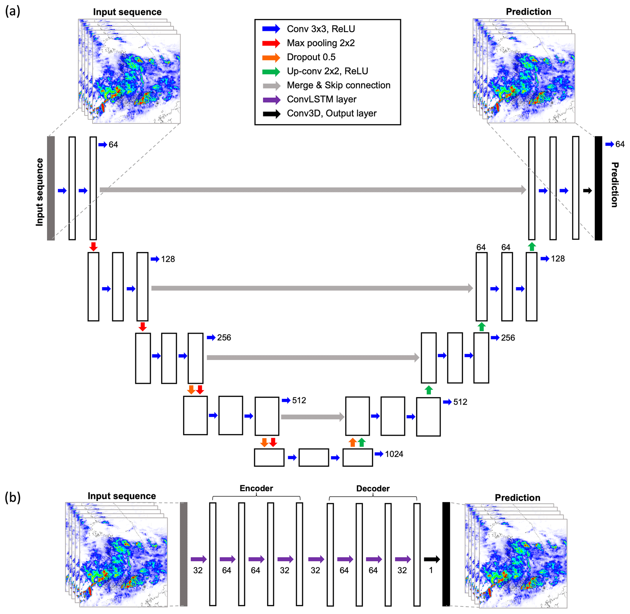
Figure 3 The structure of (a) U-Net and (b) convolutional long-short term memory (ConvLSTM) used in this study.

3.3 Scheme configuration

Considering these four key factors, a total of 24 experimental schemes for DL-QPN and pySTEPS were designed (Table 2). The selection of the DL model and its tuning are crucial for maximizing forecasting accuracy. U-Net and ConvLSTM, two representative models in the DL-QPN, were compared in this study. The structures of the U-Net and ConvLSTM are summarized in Fig. 3. The U-Net model uses five levels of spatial filters to utilize the different scales of hidden features (Fig. 3a). At each level, two convolutional layers with a 3 × 3 kernel were used. The number of convolutional filters varied depending on the depth of the layer. Skip connections concatenated the equal-sized shallow and deep layers. For the ConvLSTM, we adopted an encoder–decoder structure designed for video prediction (https://github.com/holmdk/Video-Prediction-using-PyTorch, last access: 16 October 2023). Several tests were conducted for ConvLSTM to determine the optimal number of layers and hidden states for the ConvLSTM layer, considering the model performance and GPU's memory capacity. Four ConvLSTM layers were used in this study with 32, 64, 64, and 32 hidden states per layer in both encoder and decoder (Fig. 3b). All models were trained with the MSE and BMSE loss functions and adaptive momentum optimizer (ADAM) with a learning rate of 0.001, widely adopted in deep-learning regression models (Kingma and Ba, 2014). The batch size was set to 1 to easily skip training when no precipitation event is in the batch. After the convolutional layers, the rectified linear unit (ReLU) was used as an activation function to model the nonlinearity of the data. Each model was trained with a maximum of 100 epochs, and the model training was terminated when the validation performance did not improve over three iterations.

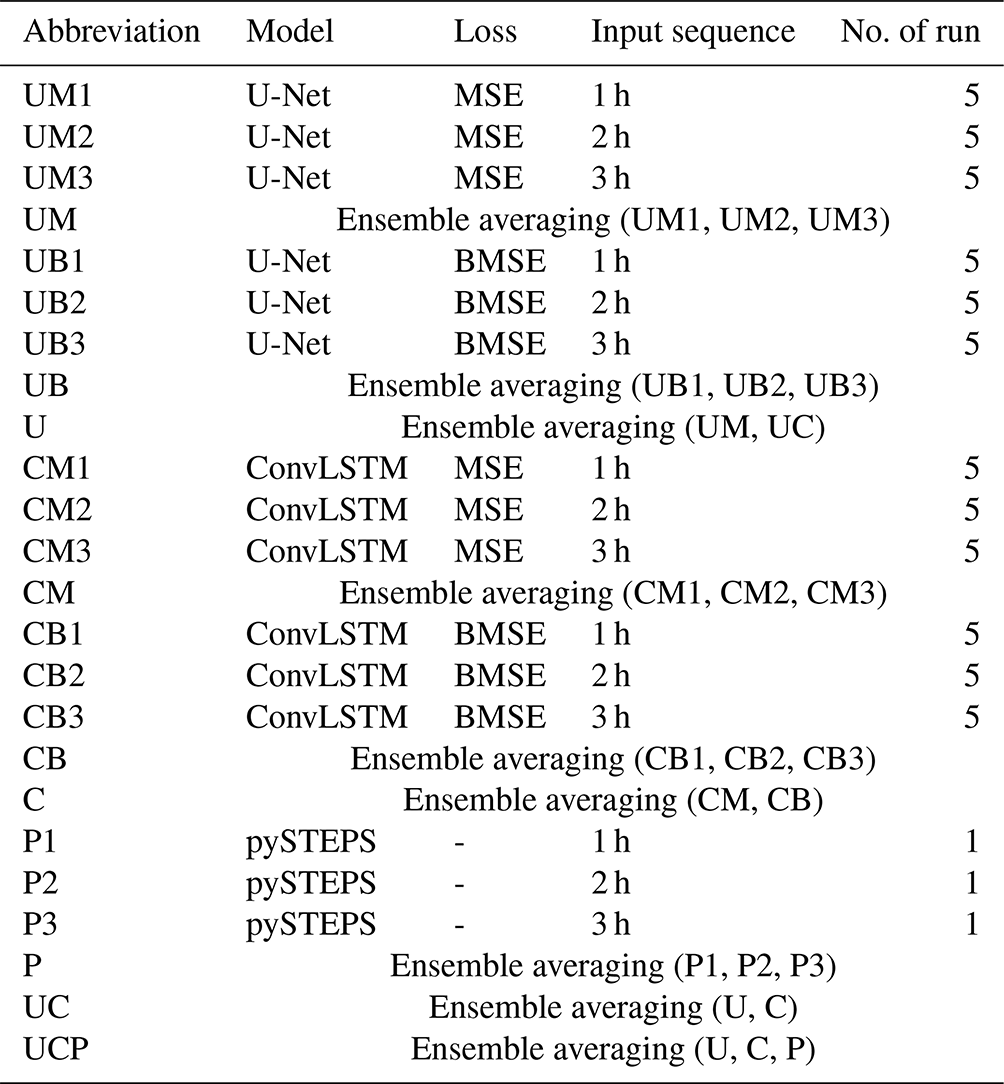
Table 2 Specifications of the schemes designed in this study with their abbreviations. “U” stands for U-Net, “C” stands for ConvLSTM, and “P” is for pySTEPS. “M” and “B” indicate MSE and BMSE loss functions, respectively. The following number is the length of the input past sequence in hours. The number of runs indicates that there are n total members to yield an average for each scheme with different random seeds to ensure stability and representativeness.

It is notable that other DL models and hyperparameters are also to be considered in addition to these four factors. The common hyperparameters for deep learning include the batch size, activation function, learning rate, and optimizer. Because finding the best set of hyperparameters is time-consuming, other combinations of hyperparameters were not considered at this time. Some recent studies have adopted generative adversarial networks (GANs) in DL-QPN (Ravuri et al., 2021; Kim and Hong, 2021). Although GANs can be expected to be a promising approach in DL-QPN, we did not compare it in this study because it is far beyond our scope owing to its complexity and diversity.

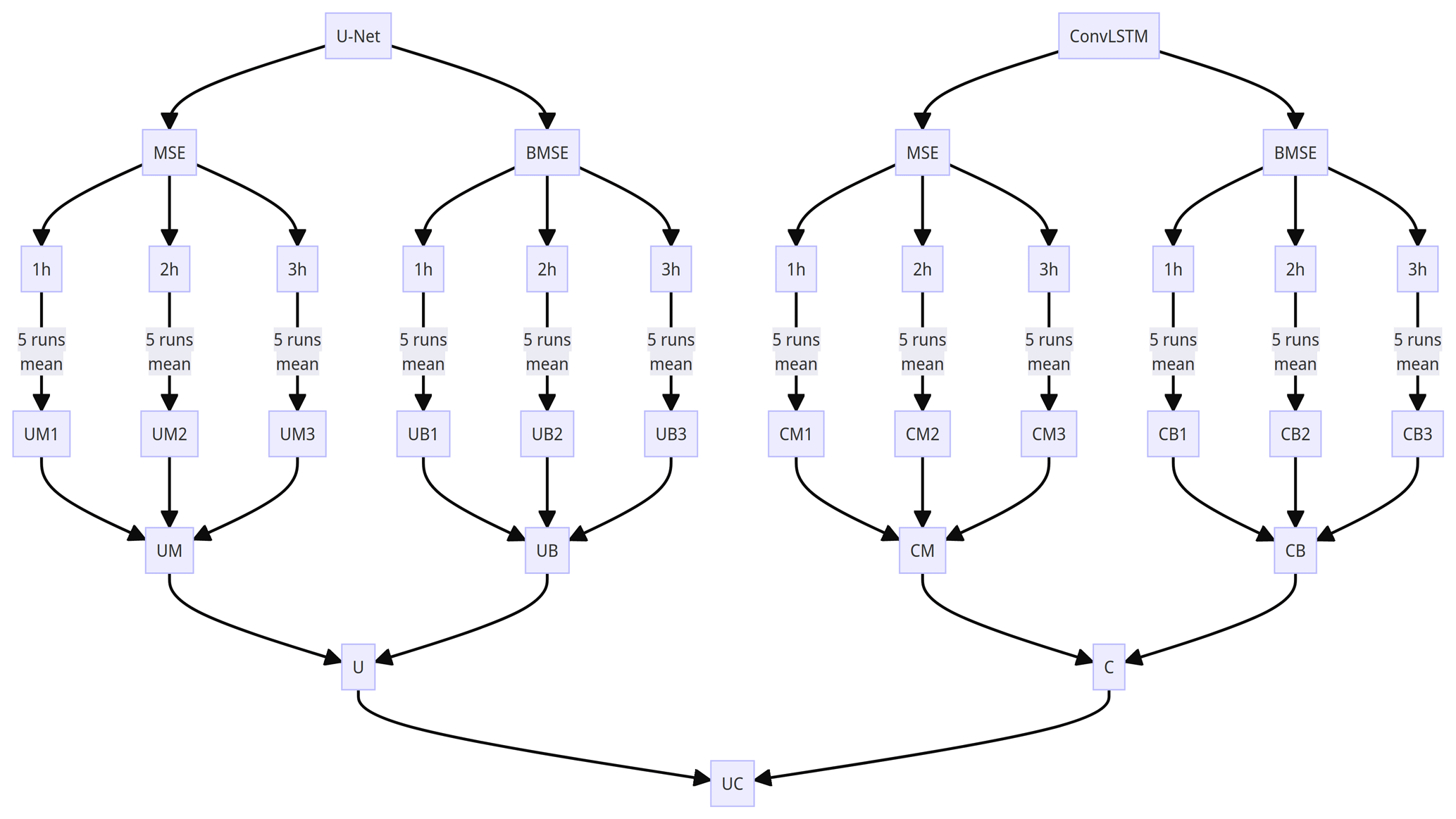
Figure 4 The infographic for overall flowchart for DL models in this study. “U” stands for U-Net and “C” stands for ConvLSTM. “M” and “B” indicate MSE and BMSE loss functions, respectively. Refer to Table 2 for each scheme.

In DL models, there are various aspects that contain randomness, such as random weight initialization or a random mini batch from the entire samples. To evaluate the model performance more reliably, we ran each scheme five times with different random seeds of 0, 999, 2023, 44 919, and 2 022 276. Starting from combining DL models (U-Net or ConvLSTM), loss functions (MSE or BMSE), and input sequence lengths (1 h, 2 h, or 3 h), a total of 12 initial schemes were generated before ensemble averaging. As each initial scheme had five runs with different random scenes, a total of 60 runs for training DL models were conducted in this study (Table 2 and Fig. 4). By aggregating five members for each scheme, each scheme can assure more stability than a single run. For example, UM1 stands for the average of U-Net trained by MSE loss with an input sequence of 1 h for five different random seeds. The average of each scheme with different input sequence lengths was again aggregated; for example, UM is the ensemble mean of UM1, UM2, and UM3. Consequently, UM is the mean of the total 15 runs, and the same is true for UB, CM, and CB. The remaining ensemble processes are similar to those in Table 2.

3.4 Evaluation

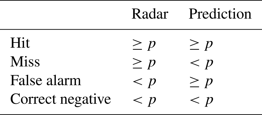
Four metrics were used to evaluate model performance: MSE, BMSE, mean bias, and the critical success index (CSI) (Table 3 and Eqs. 2–5). To exclude clear scenes from the evaluation, we only used scenes in which the number of pixels with precipitation greater than 1 mm h⁻¹ exceeded 3 % of each scene's total number of pixels. A total of 3801 scenes met this criterion during the evaluation period from 2020 to 2022, and the percentage of precipitation days was 12.73 %. We excluded precipitation of less than 1 mm h⁻¹ to avoid the effects of clear skies and radar noise. Additional thresholds of 5 and 10 mm h⁻¹ were used to account for moderate and heavy precipitation events.

Table 3 Confusion matrix for given threshold precipitation p.

Moreover, temporal analysis was conducted using summer monsoon rainfall events across the Korean Peninsula in August 2020 to examine the model performance for heavy rainfall phenomena. The summer monsoon rainfall in South Korea in 2020 lasted 54 d, from 24 June to 16 August. More than 66 % of the annual average precipitation fell during this period, with significant regional variation. In particular, 400–600 mm of rainfall fell over the southern part of the Korean Peninsula between 7 and 8 August (Lee et al., 2020; Y.-T. Kim et al., 2020). Therefore, the specific evaluation period was set up from 08:00 KST on 7 August to 20:00 KST on 8 August, including record-breaking rainfall in the southwestern region.

$$\begin{array}{}\text{(4)}& \text{mean bias}={\displaystyle \frac{\sum _{i=\mathrm{1}}^N\left(y_i-{\widehat{y}}_i\right)}{N}},\end{array}$$

where y is the reference value and $\widehat{y}$ represents the predicted value.

$$\begin{array}{}\text{(5)}& \mathrm{CSI}={\displaystyle \frac{\text{hit}}{\text{hit}+\text{miss}+\text{false alarm}}}\end{array}$$

Table 4 Quantitative performance over the summers of 2020–2022 for the 1 h prediction. Please refer to Table 2 for each scheme. The numbers after metrics indicate the thresholds of precipitation for evaluation. Upward and downward arrows indicate that the metric is better when larger and smaller, respectively. The best scores (i.e., lowest MSE and BMSE and highest CSIs) are marked in bold.

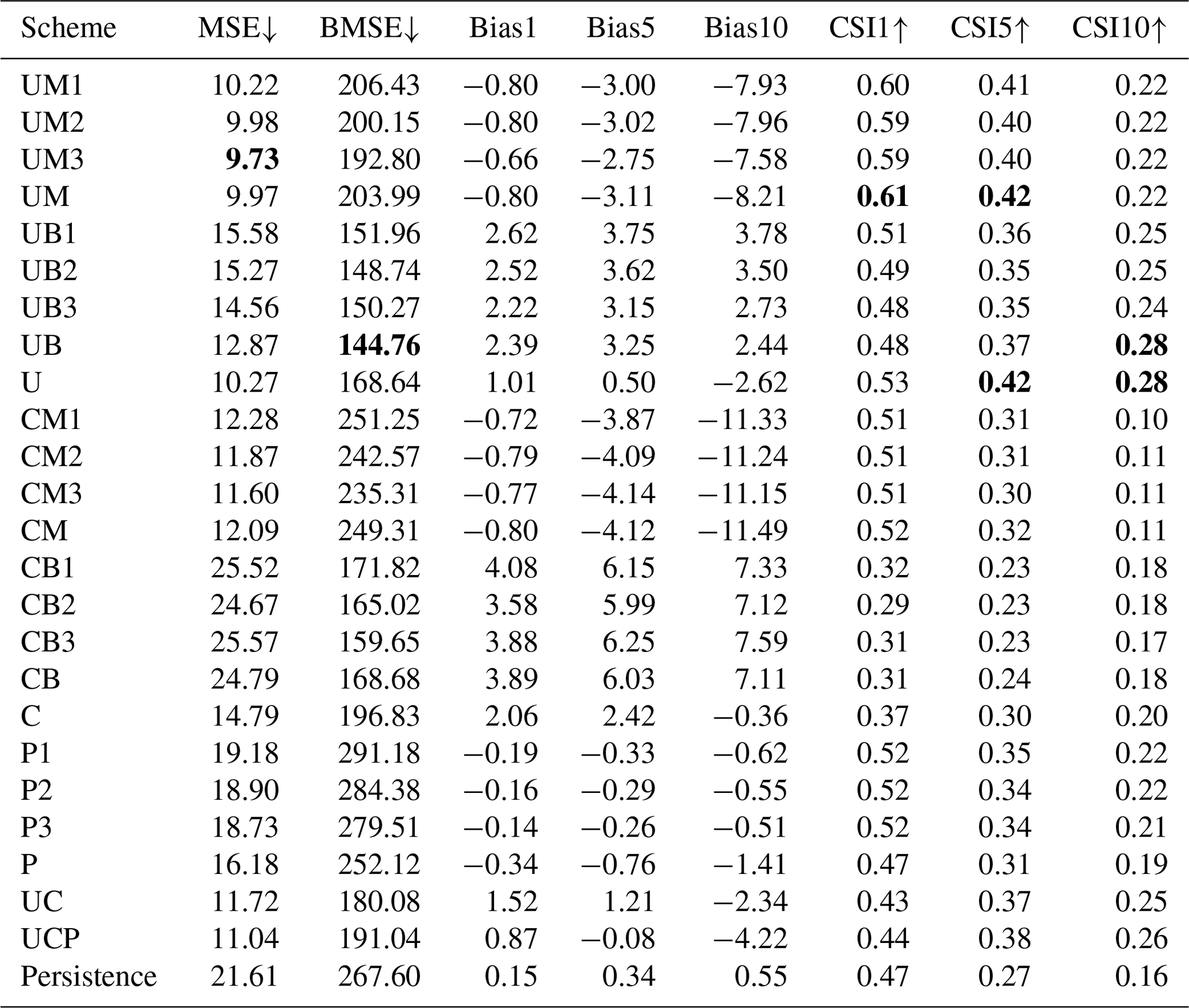
Table 5 Quantitative performance over the summers of 2020–2022 for the 2 h prediction. Please refer to Table 2 for each scheme. The numbers after metrics indicate the thresholds of precipitation for evaluation. Upward and downward arrows indicate that the metric is better when larger and smaller, respectively. The best scores (i.e., lowest MSE and BMSE and highest CSIs) are marked in bold.

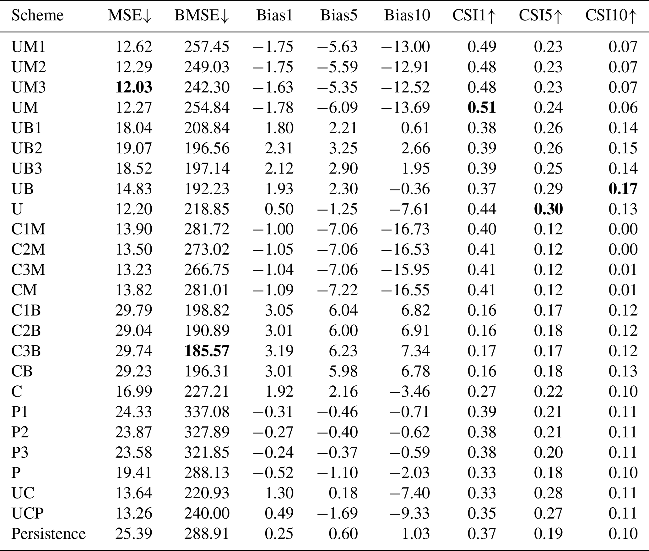
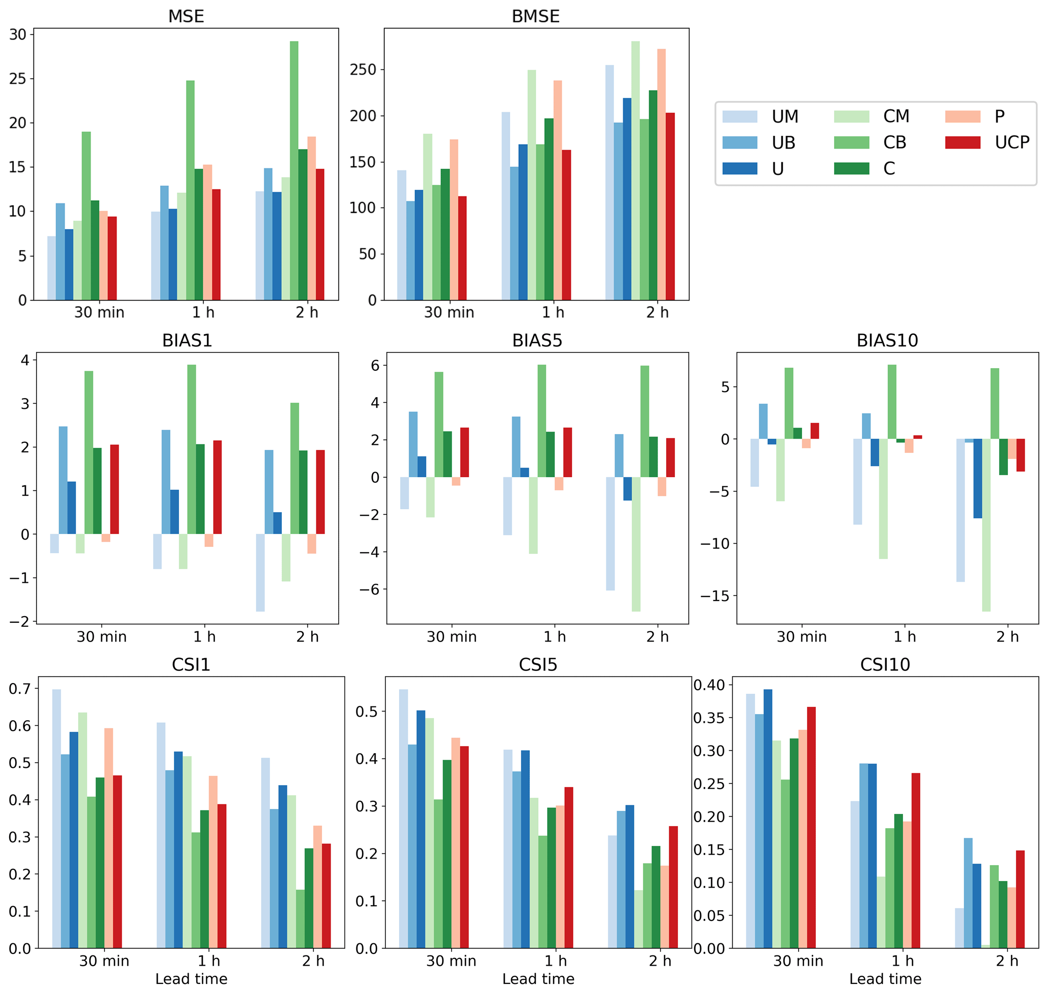
Figure 5 Quantitative performance over the summers of 2020–2022 of lead times of 30 min, 1 h, and 2 h. Please refer to Table 2 for each scheme. The numbers after the metrics indicate the thresholds of precipitation for evaluation.

4 Results

4.1 Model evaluation using precipitation events for 2020–2022

Tables 4 and 5 present the evaluation results for 1 and 2 h predictions, respectively, over June, July, and August (JJA) from 2020 to 2022. The n-hour persistence model represents a straightforward approach in which the current precipitation is assumed to persist without any change for the next n hours. A longer input sequence length generally yields lower MSE and BMSE for all schemes, with specific improvements seen for UM and CM in both prediction lead times. This trend can also be observed with UB and CB and, interestingly, in the pySTEPS non-DL model. P3 demonstrated the lowest MSE and BMSE across all P1-P3 schemes in both prediction periods, suggesting that a longer input sequence can reduce both general capitation (MSE) and high-intensity weighted metrics (BMSE). However, no significant patterns were discernible in other metrics, such as mean bias or CSI, across all schemes with varying input sequence lengths. As the ensemble mean revealed similar results to individual members with different input sequence lengths, subsequent analyses solely focused on aggregated results (i.e., UM, UB, CM, and CB), as illustrated in Fig. 5.

Distinct loss functions exert a substantial influence on every metric. Schemes with MSE loss (UM and CM) revealed a lower MSE and higher BMSE compared to BMSE scenarios (UB and CB) at both lead times, an expected outcome given they were optimized for each respective loss function (refer to Tables 4 and 5, and Fig. 5). In terms of bias, UM and CM consistently had negative values at thresholds of 1, 5, and 10 mm h⁻¹. While the magnitude of negative BIAS1 in CM was less than UM, it increased at higher thresholds as lead time extended, reaching approximately −15 mm h⁻¹ for BIAS10 in a 2 h lead time. Conversely, UB and CB generally presented positive biases except for UM with a 2 h lead time in BIAS10 (Fig. 5). This suggests that utilizing BMSE bolsters overall intensities by focusing on heavy precipitation, potentially leading to model overestimation. Equally notable is the exacerbation of underestimation in UM and CM at higher thresholds and longer lead times. Consequently, a fusion of both losses could help alleviate issues of underestimation and overestimation, as demonstrated in U and C. Figure 5 reveals that the biases of the U and C approaches are close to zero across all thresholds and lead times after aggregating MSE and BMSE. Zero bias does not inherently signify superior performance. When looked at with other metrics like MSE or CSI, it seems that the combination of MSE and BMSE successfully reduced severe underestimation and overestimation problems while keeping overall performance the same. For instance, even though U does not exhibit higher CSI across all thresholds and lead times than UM or UB, it provides a more balanced performance. There were insignificant improvements resulting from the ensemble over different input sequence lengths. Additionally, UC or UCP did not show more meaningful improvement than U. This implies that having more ensemble members with different schemes does not guarantee model improvement when the individual members do not create meaningful synergy.

Both MSE and BMSE loss functions yielded better overall metrics with U-Net than ConvLSTM. Comparisons of ensemble means of input sequence length in both 1 and 2 h predictions showed that UM and UB had lower MSE and BMSE and higher CSIs for all thresholds than CM and CB, respectively (Tables 4 and 5, Fig. 5). The performance gap between U-Net and ConvLSTM widened with increasing lead time and precipitation intensity. The disparity in bias was particularly large in ConvLSTM compared to U-Net. Moreover, when aggregating all ensemble members for each model, U consistently outperformed C. However, given the variety of possible model configurations, it should be noted that our findings do not suggest that all CNN-RNN models are inherently inferior to solely CNN models for QPN.

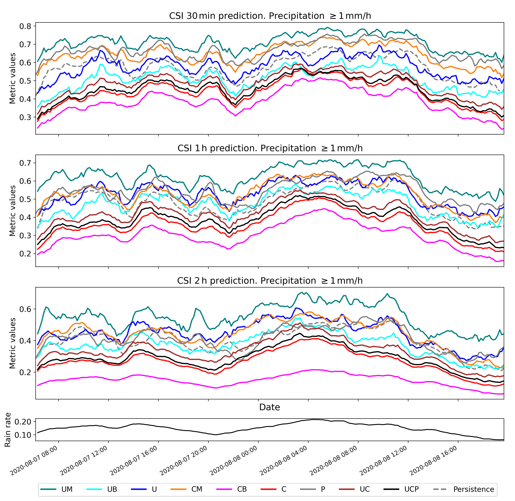
Figure 6 Comparison of CSI performance for the case of heavy rainfall over South Korea from 7 to 8 August 2020 with the 1 mm h⁻¹ threshold. Refer to Table 2 for scheme names. The bottom black line represents the ratio of precipitation pixels > 1 mm h⁻¹ for each radar scene.

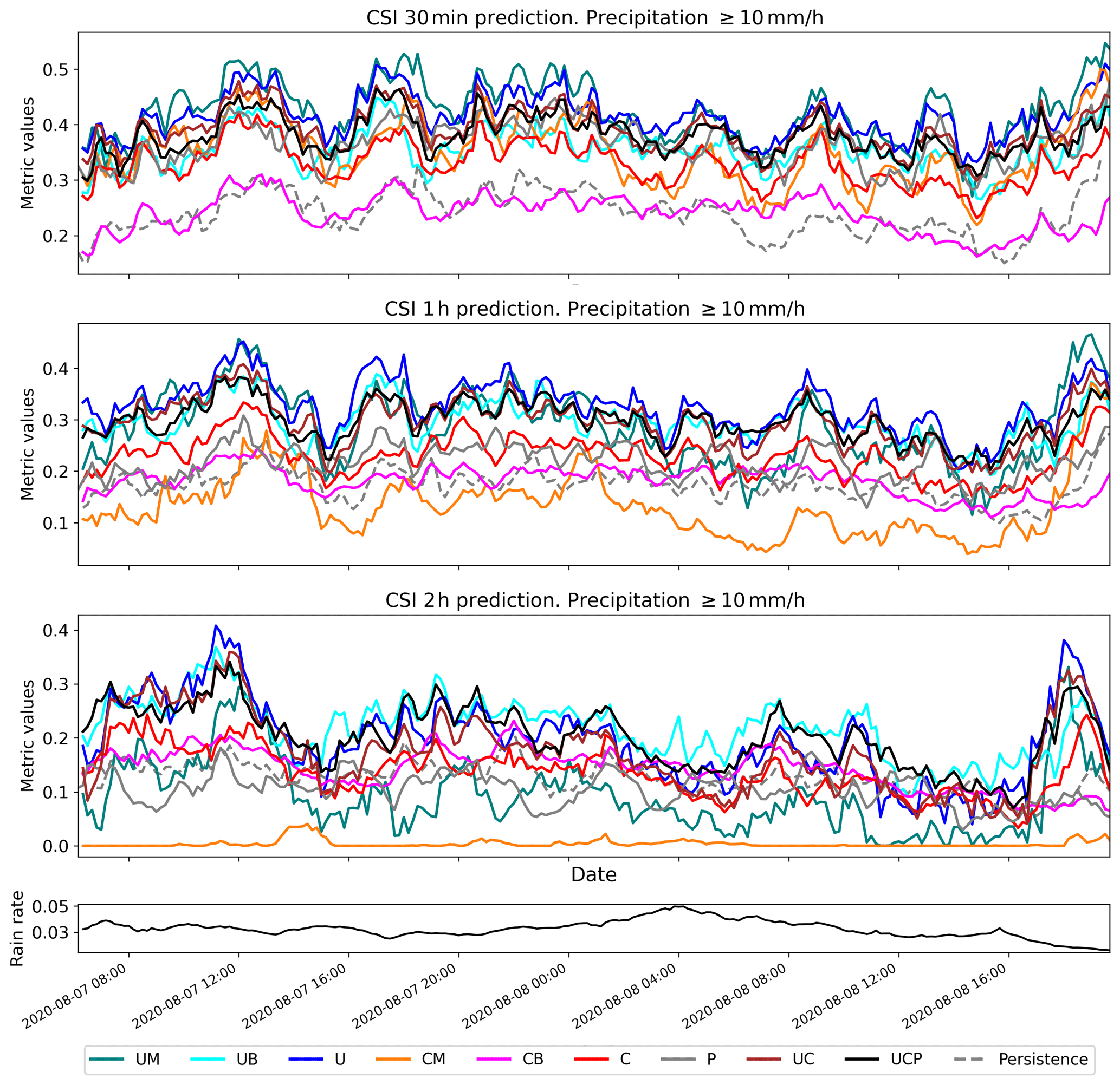
Figure 7 Comparison of CSI performance for the case of heavy rainfall over South Korea from 7 to 8 August 2020 with the 10 mm h⁻¹ threshold. Refer to Table 2 for scheme names. The bottom black line represents the ratio of precipitation pixels > 10 mm h⁻¹ for each radar scene.

4.2 Evaluation of heavy rainfall events

Figures 6 and 7 present a time series analysis of CSI1 and CSI10, respectively, for a heavy rainfall event occurring from 7 to 9 August 2020. It is important to note that the performance of all models, including persistence, was influenced by the rate of rain pixels in each scene (Fig. 6). Consequently, the performance of QPN should be interpreted in terms of the precipitation rate because the likelihood of achieving a correct prediction (i.e., CSI) increases as the area of precipitation expands (Han et al., 2023). As illustrated in Fig. 6, UM achieved the highest CSI1, whereas CB registered the poorest performance across all lead times. Echoing the long-term evaluation results from the summers of 2020–2022, UM and CM significantly outperformed UB and CB for the 1 mm h⁻¹ threshold, yielding higher CSI values. U and C, the ensembles of MSE and BMSE for each deep-learning model, demonstrated CSI1 performance roughly equivalent to the average of UM and UB and CM and CB, respectively. At the 10 mm h⁻¹ threshold, however, UM and CM's performance declined. Although UM retained competitive performance in the 30 min forecast, its skill score plummeted to the lowest level for CM in the 2 h prediction (Fig. 7). UB and CB achieved higher CSI10 than UM and CM in both 1 and 2 h predictions, implying that the benefits of using BMSE increased with longer lead times, a pattern consistent with the long-term evaluation in Fig. 5. As the CSI10 performances of UB and U were nearly identical in 30 min and 1 h predictions, U's performance in heavy precipitation seemed to be largely dictated by UB. Despite the overestimation caused by the use of BMSE, U's CSI10 did not degrade, even with the average of weaker precipitation from UM whose loss was MSE. However, due to the severe underestimation issue with UM, U's CSI10 ultimately degraded relative to UB in the 2 h prediction (Fig. 7). This pattern also aligns with Fig. 5.

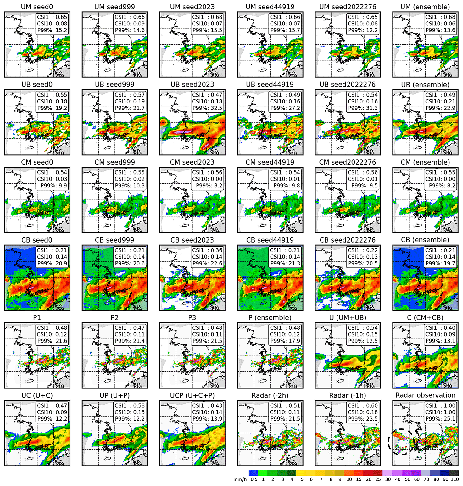
Figure 8 Comparison map for 05:00 KST on 8 August 2020 with a 2 h lead time. Refer to Table 2 for scheme names. Schemes with seed numbers are the averages of results for three scenes using 1, 2, and 3 h input sequences. CSI1 and CSI10 represent the CSI scores for thresholds of 1 and 10 mm h⁻¹, respectively, while P99 % denotes the precipitation intensity at the 99th percentile of the distribution for each scene in mm h⁻¹. The dashed black circle on the radar map indicates new growing precipitation areas that have appeared beyond radar coverage.

Figure 8 provides a comparative map for each scheme's 2 h prediction for 05:00 KST on 8 August 2020. To demonstrate the sensitivity to random seeds, predictions with each seed were included. Stability over random seeds increased more significantly with U-Net than with Conv-LSTM and with MSE than BMSE, in terms of both quantitative metrics (i.e., CSI1 and CSI10) and qualitative visual interpretation. Generally, UM and CM tended to underestimate both the area and intensity of precipitation, while UB and CB generated higher intensity over a larger area. UM exhibited the best performance in CSI1, suggesting its proficiency at forecasting the overall precipitation area. In terms of CSI10, UB and CB outperformed the others, indicating the effectiveness of BMSE in forecasting areas of heavy precipitation. Although pySTEPS appeared to closely mimic actual radar observations, the location of the forecast was simulated faster (more eastward) than the actual position. Moreover, no forecast results were available for the western part of the map because its prediction was based on a calculated wind vector. In contrast, some deep-learning models simulated rainfall over the Yellow Sea (black circle in the radar observation map), indicating the superior capabilities of these models in forecasting areas of precipitation. In terms of the 99th percentile (P99 %) precipitation intensity for each scene in Fig. 8, the results from the ensemble generally show a decreased P99 %. Even U showed a lower P99 % than UM despite being ensembled with UB. As Franch et al. (2020) pointed out, the ensemble might attenuate peak intensity. All deep-learning models produced blurred predictions compared to pySTEPS or radar observations, showing the common limitation that is discussed in Sect. 5.2.

5 Discussion

5.1 Performance comparison and considerations of key factors

To address data imbalance and improve skill scores, various loss functions have been considered in previous research. Our comparison of two representative losses, MSE and BMSE, revealed that each has its strengths and weaknesses. The selection of an appropriate loss function should be informed by a comprehensive evaluation of QPN results. Optimal loss functions may vary depending on the specific objectives as it provides guidance to DL modeling. For instance, if the model's focus is on severe weather, BMSE can be weighted to emphasize high intensities. In cases where the area of precipitation over a certain threshold is of key interest, a modified CSI loss can be used (Ko et al., 2022). As a single metric cannot fully evaluate a model, combinations of different losses can also be explored. Alternatively, the ensemble approach analyzed in our study can leverage different loss functions to create a synergistic effect for QPN.

In this study, U-Net consistently outperformed ConvLSTM in various respects, both in long-term evaluation and in a single heavy rainfall event. This finding is in line with previous research (Ayzel et al., 2020; Ko et al., 2022; Han et al., 2023). Additionally, U-Net demonstrated more stability across different random seeds than ConvLSTM (Fig. 8). Contrary to the widespread expectation that DL models powered by RNN would excel in time series forecasting, it was found that a model relying solely on CNN can perform better. However, this does not imply that all models using RNN structures are inferior to full CNN models. Considering the wide range of U-Net and ConvLSTM variants, there could be potential for RNN-powered models to exhibit superior results. Lastly, the input sequence length did not significantly impact the results compared to other factors in this study. Nevertheless, sequence length should still be carefully considered because DL-QPN relies significantly on past information. In other DL models and QPN designs, input sequence length may have a greater impact than it did in this study; therefore, we continue to regard this as a key factor in DL-QPN.

Due to the inherent randomness and stochastic nature of deep learning, modeling and evaluation need to be carefully conducted, taking into account relevant factors. As demonstrated in Fig. 8, results can vary for each run with a different random seed. Thus, stability should be a priority when developing a DL-QPN model, a point often overlooked in previous studies. By treating each run as an ensemble member, we can avoid unstable results under varying conditions of randomness.

5.2 Common drawbacks of DL-QPN

In this study, all DL-QPN schemes demonstrated a dwindling intensity problem as the lead time increased for both the long-term experiment and the heavy rainfall event. Previous studies have also reported deformation and significant blurring effects in DL-QPN models (Trebing et al., 2021; Ayzel et al., 2020; Shi et al., 2015), which is also found in Fig. 8. Ravuri et al. (2021) introduced Deep Generative Models of Rainfall (DGMR) to provide realistic rainfall prediction maps. While DGMR reduced the blurring effect by leveraging GAN, it did not perform better than U-Net in terms of CSI (Ko et al., 2022).

Regarding the typical limitations of DL-QPN, the following two factors may play a significant role: (1) the uneven distribution of precipitation and the sparsity of precipitation events and (2) the dynamic movement of the atmosphere. A substantial issue with DL-QPN is the skewed distribution of precipitation towards weak intensities (Adewoyin et al., 2021; Chen and Wang, 2022; Shi et al., 2017). Even after rejecting radar scenes when precipitation event was too weak during the sampling phase, the pixel-level distribution remained skewed towards the weak range. The sparsity of precipitation events is also strongly related to data imbalances. Because most pixels have no radar signal, the background of the weather radar mainly consists of zero values. This sparsity distinguishes the DL-QPN from general video prediction and makes the model susceptible to the prediction of underestimated results. Data augmentation or patch-level sampling can be used during the sampling phase to reduce data imbalance and sparsity. Some loss functions have also been used to solve this skewed distribution during the model training phase (Ravuri et al., 2021; Shi et al., 2017; Ko et al., 2022).

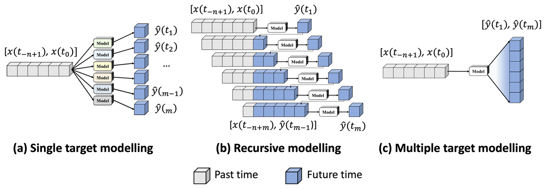
Figure 9 Three forecasting designs in DL-QPN with radar sequence: (a) single, (b) recursive, and (c) multiple predictions.

Because the DL-QPN deals with very dynamic atmospheric data, the mismatched position between past and future sequences can result in significantly degraded performance as the forecasting time increases. The DL-QPN does not explicitly learn the movement of the precipitation cells. Because convolutional filters in a single layer cannot link remote information beyond the kernel size, multiple layers gradually extend the receptive field of interest. However, even with multiple layers, the model may fail to simulate a future precipitation cell whose position is too far from its origin. This limitation might be improved by the attention techniques that enable the model to identify high relationships between input and prediction over a global area.

Although recent studies on DL-QPN have reported that they achieve better performance than traditional models with end-to-end learning, it is crucial to investigate how to fully exploit precipitation characteristics in DL-QPN. The properties of each precipitation cell can be explicitly fed into the model to successfully simulate the relationship between the precipitation cells across different time steps. In a similar context, there is ample room to contribute to radar-based DL-QPN using additional input variables, such as atmospheric instability indices, temperature, vertical humidity profiles, wind vectors, and NWP-predicted precipitation. Although some previous studies have attempted to fuse heterogeneous datasets for DL-QPN (F. Zhang et al., 2021; Adewoyin et al., 2021; Bouget et al., 2021), further research is required to determine their contribution and develop a synergetic model to maximize the multimodal dataset, instead of just stacking the variables as input features.

5.3 Other factors to consider

In addition to the four key factors investigated, there are other factors that could be considered. First, there are different prediction designs other than the multi-to-multi approach used in this study: three representative approaches are summarized from the literature (Table 2 and Fig. 9). In a single prediction, each model individually predicts each time step. Because of its simplicity and good performance focusing on a single lead time, image-to-image DL-QPN with radar (Chen et al., 2020) and image-to-point QPN with radar (Y. J. Kim et al., 2020) adopt this method. A single prediction employs n distinct models for m time steps (Fig. 9a). As shown in Fig. 9b, recursive prediction only considers the next time step. The predicted output of the first future time step was fed into an input sequence to predict the next time step, and this process was repeated iteratively to forecast longer lead times. Ayzel et al. (2020) proposed RainNet v1.0, with a recursive approach, using the previous six sequences to forecast up to 12 future sequences with an interval of 5 min. Because the recursive model only considers the next time step, it is expected to yield accurate predictions. However, the primary disadvantage of this method is the accumulation of errors with increasing lead time because more predicted results with uncertainty are used as input data. In the multiple prediction, a model simultaneously forecasts all future sequences. This design has been widely adopted for DL-QPN using a weather radar (Kim and Hong, 2021; Ravuri et al., 2021; Shi et al., 2015; Shi et al., 2017; Franch et al., 2020). A multiple prediction model can generate m time steps, as shown in Fig. 9c. Because a multiple prediction model is calibrated for various lead times by minimizing the overall loss, its performance may be degraded for a particular lead time. Although only multiple prediction was evaluated in this study due to its popularity, other approaches may also be considered based on the specific goal of each model. Additionally, there is room for the aggregation of different prediction designs to create synergy among them.

As precipitation is calculated from radar reflectivity, direct prediction of the original signal can also be considered. Some previous studies utilized radar reflectivity in DL-QPN (Bonnet et al., 2020; Lepetit et al., 2021; Albu et al., 2022; Han et al., 2022). To our knowledge, there have been few studies comparing radar reflectivity and precipitation intensity directly in DL-QPN. In this study, we chose to forecast precipitation intensity because our final interest is in the strength of the precipitation. However, as the precipitation intensity can be converted from predicted reflectivity, further investigation is needed in the future to find a better skill score.

5.4 Novelty and limitations

This study conducted a comprehensive comparison of the DL-QPN. The major novelties of this study are summarized as follows. First, we categorized and investigated four critical factors of DL-QPN. While most previous DL-QPN studies have focused on DL models, there has been a dearth of research on other factors to be considered. Second, a long-term evaluation was conducted for 3 years during the summer. This long-term evaluation provided helpful information from an operational perspective of DL-QPN. Randomness in the training phase, such as initialization of weights, was addressed for the first time in this study. Stability is one of the most important aspects of the operational model for disaster forecasting; however, this was rarely considered in previous studies. By running each DL scheme five times with different random seeds, we could examine the stability of each scheme and test the effect of ensemble aggregation. The ensemble with different DL-QPN schemes and even with a non-DL model was also newly conducted in this study, showing the potential of the ensemble approach. With advanced approaches to adjusting the optimal weights for each ensemble member, such as stacking ensemble (Cho et al., 2020), further improvements are expected. Lastly, we summarize the common drawbacks of DL-QPN and discuss their possible causes.

Despite the innovations in investigating key factors in DL-QPN, several limitations remain. One of the significant limitations of this study is the lack of investigation of more loss functions beyond MSE and BMSE. In addition to L1 and L2 losses, several loss functions have been suggested for DL-QPN, such as logcosh (Ayzel et al., 2020; Cuomo and Chandrasekar, 2021) or adversarial loss using GAN (Ravuri et al., 2021; Kim and Hong, 2021). Although the loss function in the DL-QPN is of the utmost importance, it is beyond the scope of this study, as there are too many aspects to cover in a single paper. Another limitation is the small study area. To generalize the research findings, it would be ideal for examining several study areas with different environments if possible. Some recent studies have attempted to extend their study areas using different radar data (Ravuri et al., 2021; Zhang et al., 2023). Consequently, it is highly expected to evaluate models over multiple study areas in the future to increase operational generalizations. As DL-QPN has garnered significant attention in recent years, advanced models have been continuously suggested, including GANs (Ravuri et al., 2021; Choi and Kim, 2022; Kim and Hong, 2021), latent diffusion (Leinonen et al., 2023), Transformer (Franch et al., 2023), simpler yet better video prediction (Han et al., 2023), and NowcastNet (Zhang et al., 2023). Despite the importance of using state-of-the-art (SOTA) models in DL-QPN, at this moment they are out of the scope of this paper due to their complexity, limitations of implementation, or issues of code availability. A comprehensive benchmark for different SOTA models is anticipated in our future studies, and if possible determining their optimal ensemble for further improvement will also be one of our future areas of investigation.

6 Conclusion

This paper summarizes and compares the effects of the four critical factors in the DL-QPN. As previous studies mainly focused on developing DL models with less investigation of other considerations, we expect this study to contribute to future DL-QPN studies by drawing attention to other essential factors. We evaluated various DL schemes, considering the deep learning model, input sequence length, loss function, and ensemble method. Through our quantitative and qualitative comparisons, we found that the U-Net model with the MSE loss function appeared to be the optimal combination for weak precipitation prediction in this study, while the BMSE was effective for heavy precipitation (≥ 10 mm h⁻¹). In general, there was a weak tendency for longer past sequence lengths to yield lower MSE and BMSE for both DL models, but there was little difference in terms of the CSI. After running experiments five times for each scheme, we determined that U-Net and MSE were more stable than ConvLSTM and BMSE in terms of randomness. The aggregation of different schemes resulted in balanced skill scores across multiple metrics, especially when MSE and BMSE were combined. Common issues with DL-QPN include underestimation as the lead time gets longer and the production of smoothed spatial patterns. These drawbacks are likely due to the skewed distribution of weak intensity and the sparsity of precipitation events. They are expected to be mitigated with the implementation of an improved sampling strategy and the use of various loss functions beyond MSE or BMSE.

While our study provided a comprehensive comparison of key factors in DL-QPN, it also underscored the need for continued exploration. Areas for future research include investigating more advanced loss functions, broadening the study areas to diverse environments for greater generalization, and comparing SOTA models. Furthermore, the potential of ensemble approaches for further enhancing the performance of DL-QPN models offers promising opportunities for future investigation. Ultimately, our study points out the importance of looking at DL-QPN as a whole, not just focusing on creating DL models, and recognizing the need to consider many factors that affect precipitation nowcasting.