Customized deep learning for precipitation bias correction and downscaling

Systematic biases and coarse resolutions are major limitations of current precipitation datasets. Many deep learning (DL)-based studies have been conducted for precipitation bias correction and downscaling. However, it is still challenging for the current approaches to handle complex features of hourly precipitation, resulting in the incapability of reproducing small-scale features, such as extreme events. This study developed a customized DL model by incorporating customized loss functions, multitask learning and physically relevant covariates to bias correct and downscale hourly precipitation data. We designed six scenarios to systematically evaluate the added values of weighted loss functions, multitask learning, and atmospheric covariates compared to the regular DL and statistical approaches. The models were trained and tested using the Modern-era Retrospective Analysis for Research and Applications version 2 (MERRA2) reanalysis and the Stage IV radar observations over the northern coastal region of the Gulf of Mexico on an hourly time scale. We found that all the scenarios with weighted loss functions performed notably better than the other scenarios with conventional loss functions and a quantile mapping-based approach at hourly, daily, and monthly time scales as well as extremes. Multitask learning showed improved performance on capturing fine features of extreme events and accounting for atmospheric covariates highly improved model performance at hourly and aggregated time scales, while the improvement is not as large as from weighted loss functions. We show that the customized DL model can better downscale and bias correct hourly precipitation datasets and provide improved precipitation estimates at fine spatial and temporal resolutions where regular DL and statistical methods experience challenges.

1 Introduction

Precipitation is a major component of the hydrological cycle and is fundamentally important for many applications, such as water resources planning and management, disaster risk management, and agriculture, amongst many others. Due to the limited coverage of ground-based rain gauges, numerous gridded precipitation datasets have been developed over the past decades, including gauge-based, satellite-based reanalysis products, and merged products (Beck et al., 2019a; Sun et al., 2018). These datasets are different in terms of data sources, coverage, spatial and temporal resolution, and algorithms (see Sun et al., 2018 for a review), which provide a potential source of information to regions where conventional in situ precipitation measurements are lacking (Sun et al., 2018).

Gridded precipitation datasets have proven to be useful across a wide range of research fields, including climate trends and extreme precipitation (Bhattacharyya et al., 2022; DeGaetano et al., 2020; Fischer and Knutti, 2016; Kim et al., 2019; King et al., 2013), droughts and floods monitoring (Aadhar and Mishra, 2017; Peng et al., 2020; Suliman et al., 2020; Zhong et al., 2019), and driving hydrological models (Raimonet et al., 2017; Xu et al., 2016). However, many studies have identified that these gridded precipitation datasets include substantial biases in certain aspects compared to in situ observations (Aadhar and Mishra, 2017; Ashouri et al., 2016; Bitew and Gebremichael, 2011; Cavalcante et al., 2020; Jiang et al., 2021; Jury, 2009; Rivoire et al., 2021; Sun et al., 2018; Tong et al., 2014; Xu et al., 2016; Yilmaz et al., 2005). For example, Ashouri et al. (2016) evaluated the performance of NASA's Modern-era Retrospective Analysis for Research and Applications (MERRA) precipitation reanalysis dataset and found that MERRA tends to overestimate the frequency at which the 99th percentile of precipitation is exceeded and underestimate the magnitude of extremes, especially over the Gulf Coast regions of the USA. Furthermore, spatial resolution for most of these gridded precipitation datasets is relatively coarse for local scale applications (mostly above 0.25^∘, Sun et al., 2018). Therefore, the gridded precipitation datasets require bias correction and downscaling (Duethmann et al., 2013; Emmanouil et al., 2021; Mamalakis et al., 2017; Seyyedi et al., 2014).

Bias correcting and downscaling gridded precipitation data is challenging due to its complex characteristics (e.g., highly skewed unbalanced features, and complex spatiotemporal structure). Various approaches have been developed to tackle this issue, including traditional quantile mapping (QM)-based bias correction and downscaling methods (e.g., Cannon et al., 2015; Panofsky and Brier, 1968; Thrasher et al., 2012; Wood et al., 2002) and recent machine learning-based approaches such as random forests (X. He et al., 2016; Legasa et al., 2022; Long et al., 2019; Mei et al., 2020; Pour et al., 2016), support vector machines (Tripathi et al., 2006) and artificial neural networks (Schoof and Pryor, 2001; Vandal et al., 2019). Recently, advances in deep learning have made a significant impact on many fields and have been proven superior to traditional machine learning methods because of their powerful abilities to learn spatiotemporal feature representation in an end-to-end manner (Ham et al., 2019; Reichstein et al., 2019; Shen, 2018). In particular, deep learning (DL) with convolutional neural network (CNN) types of approaches have achieved notable progress in modeling spatial context data (LeCun et al., 2015) and have been used for bias correcting and downscaling low spatial resolution data (Kumar et al., 2021; Sha et al., 2020a, b; Vandal et al., 2018b; Wang et al., 2021; Xu et al., 2020), climate model outputs (François et al., 2021; Liu et al., 2020; Pan et al., 2021; Rodrigues et al., 2018; Wang and Tian, 2022), reanalysis products (Baño-Medina et al., 2020; Sun and Tang, 2020), and weather forecast model outputs (Harris et al., 2022; Li et al., 2022). While these studies have indicated many promising strengths and advantages over traditional downscaling and bias correction approaches, most of them have difficulties capturing local small-scale features such as extremes for an unseen dataset. For example, Baño-Medina et al. (2020) designed different DL configurations with a different number of plain CNN layers to bias correct and downscale daily ERA5-Interim reanalysis from 2^∘ spatial resolution to 0.5^∘, and the overall performance is still marginal compared with simple generalized linear regression models and highly underestimated precipitation extremes. Harris et al. (2022) developed a generative adversarial networks (GANs) architecture to bias correct and downscale weather forecast outputs and found that it is more challenging to account for forecast error (or bias) in a spatially coherent manner compared to the pure downscaling problem (Kumar et al., 2021; Sha et al., 2020a, b; Vandal et al., 2018b; Wang et al., 2021; Xu et al., 2020). The reason for that may be due to the sparsity of training data on extreme events. Deep learning (DL) models, however, need large training data in order to obtain a better regularization model for rare events in the unseen dataset.

Customized DL models have been proposed to generate physically consistent results and have better generalization ability for out-of-pocket datasets in the earth and environmental science field, which include incorporating customized loss functions (Kashinath et al., 2021), inputs from physically relevant auxiliary predictors (i.e., covariates) (Li et al., 2022; Rasp and Lerch, 2018), and customized multitask learning (Ruder, 2017). For example, Daw et al. (2017) indicated success in lake temperature modeling by incorporating a physics-based loss function into the DL objective compared to a regular loss function. Li et al. (2022) used a CNN-based approach to postprocess numerical weather prediction model output and found that the use of auxiliary predictors greatly improved model performance compared with raw precipitation data as the only predictor. A multitask model is trained to predict multiple tasks that are driven by the same underlying physical processes and thus has the potential to learn to better represent the shared physical process and better predict the variable of interest (Ruder, 2017). Multitask models have proven effective in several applications, including natural language processing (Chen et al., 2014; Seltzer and Droppo, 2013), computer vision (Girshick, 2015), as well as hydrology (Sadler et al., 2022). In addition, most of the previous bias correction and downscaling studies focused on the daily time scale (Baño-Medina et al., 2020; François et al., 2021; Harris et al., 2022; Kumar et al., 2021; Liu et al., 2020; Pan et al., 2021; Rodrigues et al., 2018; Sha et al., 2020a; Vandal et al., 2018b; Wang et al., 2021). However, the distribution of hourly precipitation data within a day is more important than daily or monthly aggregations for impacts and risks from warming-induced precipitation changes (Chen, 2020). Traditional DL loss functions have difficulties handling hourly precipitation data that are highly unbalanced with many zeros and highly positively skewed for nonzero components. Therefore, customized DL with a weighted loss function to better balance nonzero components has the potential to improve the DL model performance. Besides the primary task of downscaling and bias correction, adding a highly relevant classification task has the potential to improve DL model performance on the primary task. Incorporating covariates selected based on precipitation formation theory (cloud mass movement and thermodynamics) also have the potential to improve precipitation downscaling and bias correction.

In this study, we will explore customized DL for precipitation bias correction and downscaling, aiming to take a step forward to address the current challenges described above. We designed a set of experiments to address this hypothesis using the Modern-Era Retrospective analysis for Research and Applications Version 2 (MERRA2) reanalysis and the Stage IV radar precipitation data. The structure of this paper is organized as follows: Sect. 2 introduces data and study area, Sect. 3 introduces the methodology, including the deep learning architecture and experimental designs for different scenarios, and a traditional bias correction approach as a benchmark, Sect. 4 presents results, discussion and conclusions are provided in Sects. 5 and 6, respectively.

2 Data and study area

MERRA2 is a state of the art global reanalysis product generated by the NASA Global Modeling and Assimilation Office (GMAO) using the Goddard Earth Observing System version 5 (GEOS-5), and was introduced to replace and extend the original MERRA dataset (Reichle et al., 2017). It incorporates new satellite observations through data assimilation and benefits from advances in the GEOS-5 (Reichle et al., 2017). There are 2 datasets available for hourly total precipitation (P) from the MERRA2 reanalysis product: the model analyzed precipitation computed from the atmospheric general circulation model and the observation-corrected P (Reichle et al., 2017). Both have a spatial resolution of 0.5^∘ in latitude and 0.625^∘ in longitude (∼ 50 km). MERRA2 observation-corrected precipitation has been used extensively in hydro-climatological analysis and modeling (Chen et al., 2021; Hamal et al., 2020; Xu et al., 2019, 2022). However, it still suffers from substantial biases (e.g., Hamal et al., 2020; Xu et al., 2019). This study bias corrects and downscales MERRA2 observation-corrected P using the Stage IV radar data (Lin and Mitchell, 2005) from the National Centers for Environmental Prediction (NCEP) as the observational reference. The Stage IV radar data has a 4 km spatial and hourly temporal resolution and covers the period from 2002 until the near present (2021 in this study). Stage IV radar was generated by merging data from 140 radars and about 5500 gauges over the continental USA (Lin and Mitchell, 2005; Nelson et al., 2016). Stage IV provides highly accurate P estimates and has therefore been widely used as a reference for evaluating other P products (e.g., Aghakouchak et al., 2011, 2012; Beck et al., 2019b; Habib et al., 2009; Hong et al., 2006; Nelson et al., 2016; Zhang et al., 2018). The Stage IV dataset is a mosaic of regional analyses produced by 12 River Forecast Centers (RFCs) and is thus subject to the gauge correction and quality control performed at each individual RFC (Nelson et al., 2016).

The bias correction and downscaling experiments were performed in the rectangle coastal area of the Gulf of Mexico covering the entire states of Alabama, Mississippi, and Louisiana, and parts of neighbor states in the USA, ranging from 94.375^∘ W to 85.0^∘ W in longitude and from 29.0^∘ N to 35.0^∘ N in latitude. The study area falls into the humid subtropical climate and is highly influenced by extreme P events such as convective storms and hurricanes.

3 Methodology

3.1 Customized DL approaches

This section first presents a brief description of a DL approach, namely, Super Resolution Deep Residual Network (SRDRN). Then, multitask learning and customized loss functions are introduced based on the SRDRN architecture to construct customized DL approaches. Finally, we designed different modeling experiments, which include different combinations of multitask learning, customized loss functions, and P covariates as predictors, in order to evaluate the added values of each component of the customized DL approaches.

3.1.1 SRDRN model

The SRDRN model is an advanced deep CNN type architecture and has been tested for downscaling daily P and temperature through synthetic experiments (Wang et al., 2021) and for bias correcting near-surface temperature simulations from global climate models (Wang and Tian, 2022), considerably outperforming the conventional approaches. Furthermore, it has been proved that the SRDRN is capable of capturing much finer features than shallow plain CNN architecture (Wang et al., 2021). Compared with the popular U-Net architecture (Sha et al., 2020a; Sun and Tang, 2020), the SRDRN directly extracts features on the coarse resolution input and thus can potentially decrease computational and memory complexity.

Here we provide a brief description of the SRDRN algorithm. For more details, the readers may refer to Wang et al. (2021). The SRDRN algorithm was developed based on a novel superscaling DL approach in the computer vision field (Ledig et al., 2017). Basically, the SRDRN algorithm is comprized of residual blocks and upsampling blocks with convolutional and batch normalization layers. For feature extraction, the convolutional layers apply filters to go through the input data to build a local connection within nearby grids by computing the element-wise dot product between the filters and different patches of the input. The outcome is followed by a nonlinear activation function, here parametric ReLU (He et al., 2015) in this study. Batch normalization is a technique to standardize the inputs to a layer for each mini-batch so that the learning process can be stabilized and the training of the model can be accelerated (Ioffe and Szegedy, 2015).

With convolutional and batch normalization layers, the residual blocks are designed to extract fine spatial features while avoiding degradation issues for the very deep neural network. Compared to plain CNN architectures, residual blocks can improve the performance of extensively deep networks (Silver et al., 2017) without suffering from model accuracy saturation and degradation (K. He et al., 2016) because residual blocks execute residual mapping and include skipping connections. In this study, the way that skipping connection skips layers and connects the next layers is through element-wise addition. A total number of 16 residual blocks were used in the SRDRN architecture, which makes the network very deep and able to extract fine spatial features.

The upsampling blocks are applied to increase the spatial resolution for downscaling purposes. The upsampling process is executed directly on the feature maps generated from the residual blocks, and each upsampling block is composed of one convolutional layer and one upsampling layer followed by a parametric ReLU activation function. The defaulted nearest neighbor interpolation was chosen in the upsampling layers to increase the spatial resolution, and the effects of different interpolation methods were not explored in this study. Each upsampling block sequentially and gradually increases the input low-resolution feature maps by a factor of 2 or 3. In this study, the downscaling ratio (the ratio between coarse resolution and high-resolution data) is 12, and thus we used 3 upsampling blocks with 2 blocks having a factor of 2 and 1 block having a factor of 3.

3.1.2 SRDRN model with multitask learning

We included an additional P classification task in the SRDRN model. Besides bias correcting and downscaling continuous hourly P values as a primary task, we added another task to bias correct hourly P categories. Studies have indicated that a multitask DL model could learn to better represent the shared physical processes and better predict the variable of interest (e.g., Sadler et al., 2022). As P categories and actual values are highly relevant, adding a classification task can potentially improve the DL model for bias correcting and downscaling P.

Specifically, for the SRDRN with multitask learning, one convolutional layer (256 filters and 3×3 kernels) follows the last element-wise addition operation to summarize feature maps, then the architecture splits into two sections (Fig. 1). The first section with 2 additional convolutional layers (the first one with 64 filters and the second with 4 filters) followed by the Softmax activation (Goodfellow et al., 2016) is used for bias correcting P categories as a multiclass classification task, and the other section with upsampling blocks is used for the purpose of bias correcting and downscaling hourly P. The classification task classifies the hourly P at each grid into 4 categories: 0–0.1 mm h⁻¹ as no rain, 0.1–2.5 mm h⁻¹ as light rain, 2.5–10 mm h⁻¹ as moderate rain, and > 10 mm h⁻¹ as heavy rain (Tao et al., 2016). Due to radar sensors' uncertainty in the very light rainfall, 0.1 mm h⁻¹ is commonly used as a threshold to determine if there is rain (Tao et al., 2016). As the classification task is executed on the feature maps at the coarse resolution, we aggregated Stage IV P (namely, coarsened Stage IV in this study) into the same spatial resolution as MERRA2 and classified the upscaled P data into the four groups as target labels.

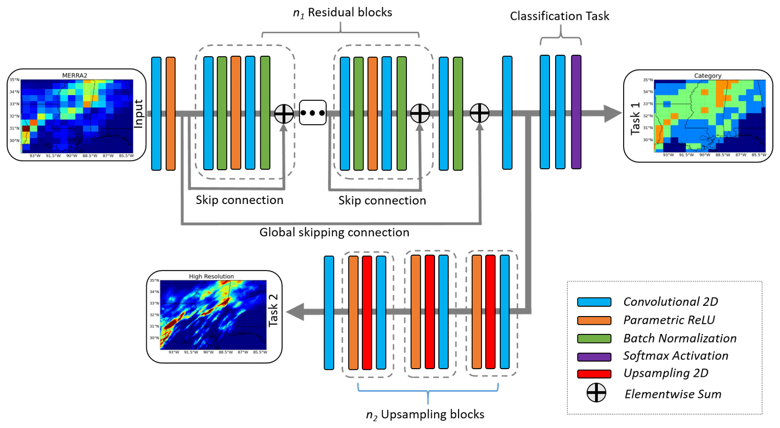
Figure 1 The customized SRDRN architecture with multitask learning, which includes the classification of P categories as an auxiliary task (task 1) in addition to downscaling and bias correcting actual P values (task 2). Note that this figure is modified from the SRDRN architecture shown in Wang et al. (2021).

3.1.3 Customized loss functions

Precipitation data is highly skewed and unbalanced, especially at an hourly time scale, which could cause the deep learning algorithm to focus more on no-rain events while ignoring heavy rain events if using regular loss functions. Here we developed a weighted mean absolute error (MAE) loss function (L_{MAE_weighted}) to balance precipitation data where weights change with precipitation values as shown by the equation

$$\begin{array}{}\text{(1)}& L_{\mathrm{MAE}\mathrm{\_}\mathrm{weighted}}={\displaystyle \frac{{\sum }_{i=\mathrm{1}}^n{w}_{\mathrm{1}}\cdot \left|y_{\mathrm{pred}}-y_{\mathrm{true}}\right|}{n}},\end{array}$$

where n is the total number of grids in a batch, w₁ is the weight for each absolute error between the model predicted value y_pred and the true value y_true. The weight w₁ changes with the actual true value y_true

$$w_{\mathrm{1}}=\left\{\begin{array}{lr}\mathrm{MIN}& y_{\mathrm{true}}\le \mathrm{MIN}\\ y_{\mathrm{true}}& \mathrm{MIN}<y_{\mathrm{true}}<\mathrm{MAX}\\ \mathrm{MAX}& y_{\mathrm{true}}\ge \mathrm{MAX}\end{array}\right.,$$

where MIN is the lowest threshold and MAX is the highest threshold for the weights. In other words, when the y_true value is below (above) MIN (MAX), w₁ equals MIN (MAX), otherwise w₁ equals y_true itself. Thus, the loss is weighted directly by the P value at the grid cell scale, which has been proven to be more effective than weighted by P bins (Ravuri et al., 2021; Shi et al., 2017). Note that all of the gridded P data, including Stage IV and MERRA2, are logarithmically transformed [i.e., $y=\log (x+\mathrm{1})$] in order to amplify the normality and reduce the skewness of P data (Sha et al., 2020a). In Eq. (1), y_true and y_pred are transformed P values. MIN was set to log(0.1+1) and MAX was set to log(100+1), where the maximum 100 mm h⁻¹ was chosen as the highest threshold before log transformation for robustness to spuriously large values in the Stage IV radar (Ravuri et al., 2021) and 0.1 mm h⁻¹ is commonly used as a threshold to determine if there is rain for radar data (Tao et al., 2016).

For the four P categories, most data fall into the no rain category (over 88 % in the coarsened Stage IV), and the minority of data fall into the heavy rain category (about 0.2 % in the coarsened Stage IV). Thus, handling class imbalance is of great importance in this situation, where the minority class for the heavy rain category is the class of most interest with respect to this learning task. The regular cross-entropy loss function for the classification task could result in the underestimation of the minority class (Fernando and Tsokos, 2021). Thus, we applied a weighted cross entropy as a loss function (L_{weighted Cross-entropy}) for the classification task in order to penalize more towards heavy rain category as follows

$$\begin{array}{}\text{(2)}& \begin{array}{rl}{L}_{\text{weighted Cross-entropy}}& =-{\sum }_{i=\mathrm{1}}^n{\sum }_{j=\mathrm{1}}^k{w}_{\mathrm{2},j}\cdot p\left(y_{i,j}\right)\\ & \cdot \log \left(q\left(y_{i,j}\right)\right),\end{array}\end{array}$$

where w_2,j denotes the weight for the jth class, p(y_i,j) represents the true distribution of the ith grid for the jth class, and q(y_i,j) represents the predicted distribution. k is the number of classes (equals 4 in this study). w_2,j was set to 1, 5, 15, and 80 for no rain, light rain, moderate rain, and heavy rain classes, respectively, which is roughly based on the opposite percentage (i.e., 1, 5, 15, 80 are approximately from the percentages of heavy, moderate, light and no rain categories, respectively) for each category of the coarsened Stage IV. As the weights for categories with rain are relatively larger than the no rain category, the loss L_{weighted Cross-entropy} is relatively large when there are discrepancies between true and predicted categories with rain, resulting in guiding the training process towards decreasing these differences with larger weights and thus better handling class imbalance issues.

3.1.4 Experimental design

To comprehensively evaluate the added value of each component of customized DL models, including weighted loss function, multitask learning, and adding covariates, we designed six scenarios (Scenario1–Scenario6 in Table 1). Scenario1 is based on the basic SRDRN architecture with hourly P from MERRA2 as coarse-resolution input, P from Stage IV as high-resolution labelled data, and regular MAE as loss function, which represents regular DL. Wang et al. (2021) used regular mean squared error (MSE) as a loss function, which works well for downscaling daily precipitation through synthetic experiments with no bias as the precipitation data were first coarsened and then downscaled into the original fine scale. However, in this study the coarse-resolution MERRA2 has substantial biases compared to Stage IV radar data, and Stage IV radar data also includes artifacts (e.g., large spurious values) (Nelson et al., 2016). The previous study has shown that the MSE loss function is more sensitive to radar artifacts than the mean absolute error (MAE) loss function (Ravuri et al., 2021). Therefore, we chose MAE as a regular loss function in this study. Scenario2 is the same as Scenario1 except using weighted MAE loss function (Eq. 1). The number of trainable parameters is the same for Scenario1 and Scenario2. Scenario3 includes the classification task, and the total loss is the combination of Eqs. (1) and (2) with a weight λ (see Eq. 3), where λ was set to 0.01 to ensure the two parts of the losses are in the same magnitude. The trainable parameters for Scenario3 increase by 30 % compared to Scenario1 and Scenario2.

$$\begin{array}{}\text{(3)}& L=L_{\mathrm{MAE}\mathrm{\_}\mathrm{weighted}}+\mathit{\lambda }\cdot L_{\text{weighted Cross-entropy}}.\end{array}$$

Table 1 Deep learning (DL) experimental design.

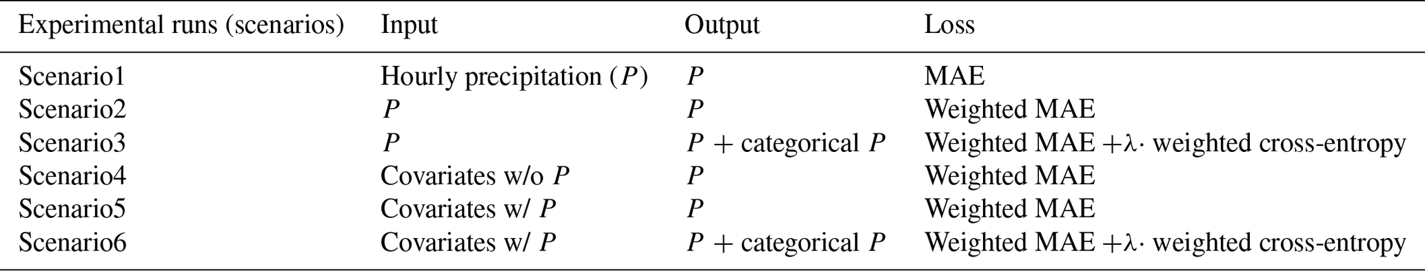
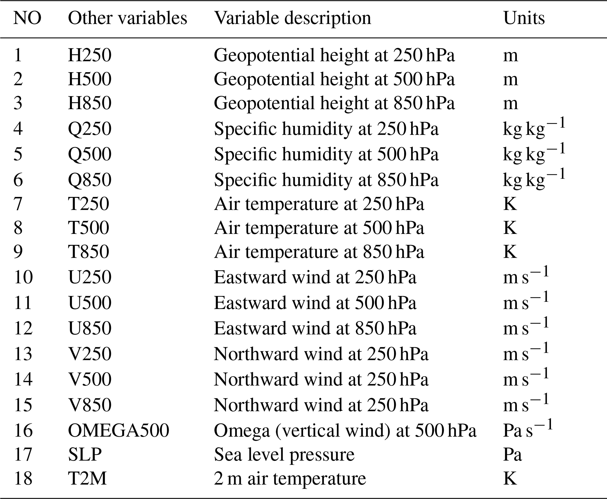
As described in Sect. 1, studies have indicated that including atmospheric covariates is helpful for estimating precipitation (e.g., Baño-Medina et al., 2020; Li et al., 2022; Rasp and Lerch, 2018). The other three scenarios also consider atmospheric covariates of P from MERRA2 as predictors, which include geopotential height, specific humidity, air temperature, eastward wind, and northward wind at three different vertical levels (250, 500, 850 hPa) (e.g., Baño-Medina et al., 2020; Rasp and Lerch, 2018) as well as vertical wind (e.g., Trinh et al., 2021) at 500 hPa (OMEGA500), sea level pressure and 2 m air temperature in a single level (e.g., Panda et al., 2022; Rasp and Lerch, 2018) (see Table 2). We chose these variables based on precipitation formation theory (cloud mass movements and thermodynamics) as well as findings from previous studies as already indicated. Comparable to a classical multiple linear regression problem, covariates are multivariable predictors, and hourly precipitation is the only dependent variable. For each covariate listed in Table 2, data normalization was executed as a data preprocessing step. Specifically, each covariate was normalized by subtracting the mean (μ) and dividing by the standard deviation (σ). Here μ and σ are scalar values that were calculated based on the flattened variable for the training dataset. During the testing period, the model prediction was made from the normalized MERRA2 with μ and σ calculated from the testing period dataset to preserve nonstationarity. Scenario4 only included atmospheric covariates without using coarse-resolution P as input and used Eq. (1) as the loss function to test whether only covariates are sufficient for estimating hourly P. The number of trainable parameters for Scenario4 is about 1 % more compared to Scenario1 and Scenario2. Scenario5 is the same as Scenario4 except including P as a predictor besides atmospheric covariates, and the number of trainable parameters is very close to Scenario4. Scenario6 is the same as Scenario5 except including the classification task with Eq. (3) as loss function and the number of trainable parameters is similar to Scenario3 (31 % greater than scenarios with no multitask learning).

Table 2 Selected atmospheric covariates for DL downscaling and bias correction.

The Adam optimization algorithm was applied to train the 6 DL scenarios with a learning rate of 0.0001 and other default values. We found that the learning rate of 0.0001 worked stably in this study through a series of experiments. The batch size for each epoch was set to 64, and the number of epochs was set to 150 for each scenario listed in Table 1. Each scenario was trained with approximately 2.5×10⁵ iterations. We frequently saved models and evaluated their performance with a validation dataset in order to choose the best model for prediction on the testing dataset. The training process was executed using NVIDIA V100 GPU provided by the NASA High-End Computing (HEC) Program through the NASA Center for Climate Simulation (NCCS) at the Goddard Space Flight Center (https://www.nccs.nasa.gov/systems/ADAPT/Prism, last access: 18 November 2022).

At the time when we conducted this study, MERRA2 and Stage IV hourly P data have a 20-year overlapping period from 2002 to 2021. We used the first 14 years (2002–2015) as the training dataset, the middle 3 years (2016–2018) as the validation dataset, and the more recent 3 years (2019–2021) as the testing dataset. Figure 2 shows the hourly mean or climatology for MERRA2 and Stage IV for training and testing datasets, as well as the mean differences between the testing and the training periods. We can tell that there are large climatology differences (or biases) between MERRA2 and Stage IV both for training and testing datasets, especially around the coastal area. Wetter conditions are observed in most of the study area in the testing period (average 0.03 mm h⁻¹) than in the training period, which is due to a higher percentage of rain (with values greater than 0.5 mm h⁻¹) during the testing period than during the training period based on analyzing the Stage IV data (Table S1 in the Supplement). This allows us to assess the extrapolation capabilities of the different methods, which is particularly relevant in a changing climate.

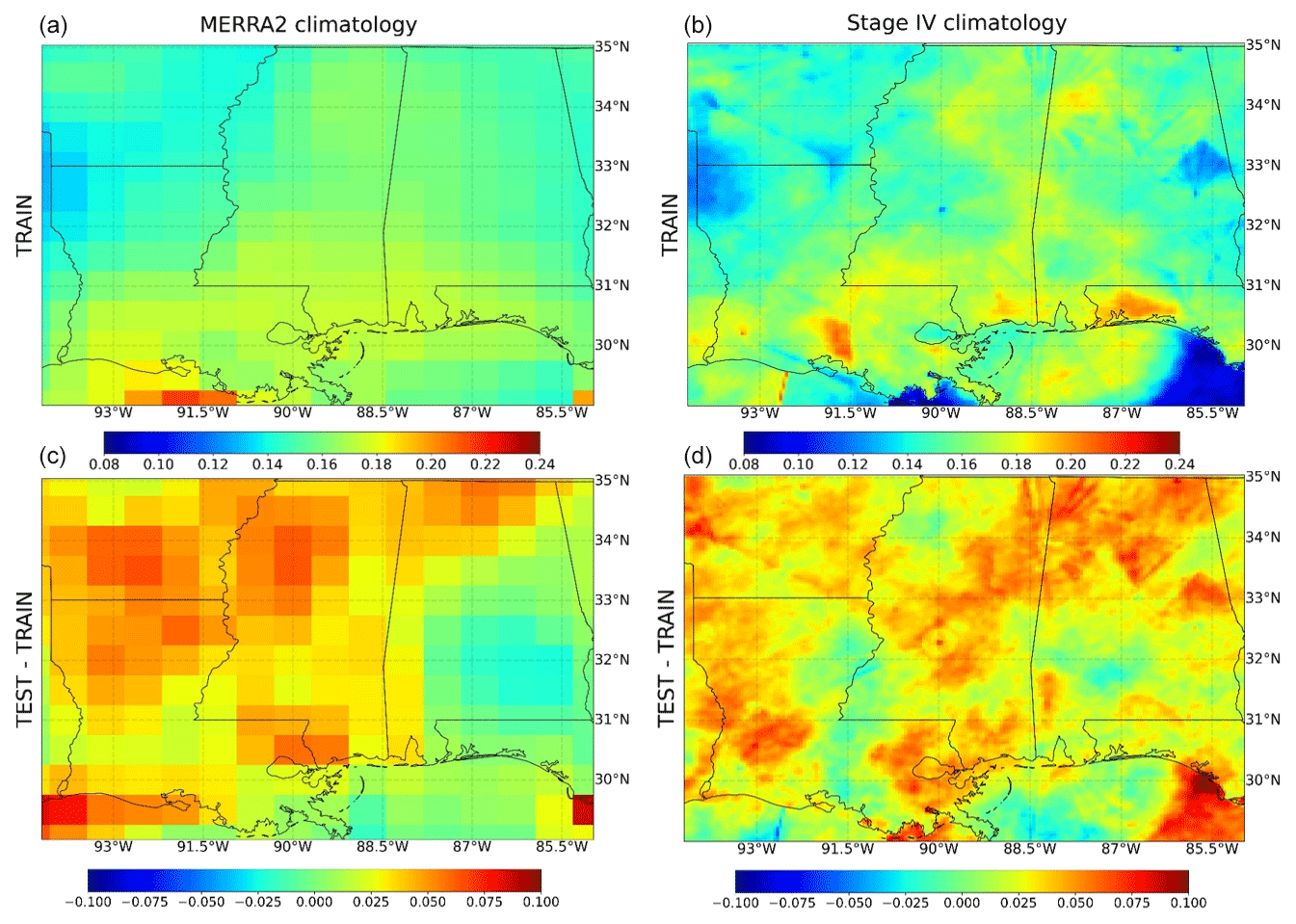
Figure 2 Climatology of hourly precipitation (in a unit of mm h⁻¹) from MERRA2 and Stage IV during the training period (2002–2015; first row) and their differences (second row) between the testing (2019–2021) and training periods.

3.2 Statistical approach

We used a widely accepted quantile delta mapping (QDM) as a benchmark approach for P bias correction. The QDM method corrects systematic biases at each grid cell in quantiles of a modeled series with respect to observed values. Compared to the regular quantile mapping method (Panofsky and Brier, 1968; Thrasher et al., 2012; Wood et al., 2002), QDM also applies a relative difference between historical and future climate data (here, training and testing periods). Thus it is capable of preserving the trend of the future climate (Cannon et al., 2015), which is critical for this study as there are substantial differences between the precipitation during the training (2002–2015) and testing (2019–2021) periods (see Fig. 2). This approach has been widely used to bias correct climate variables, including P, which indicated better performance compared to the other bias correction approaches (Cannon et al., 2015; Eden et al., 2012; Kim et al., 2021; Tegegne and Melesse, 2021; Tong et al., 2021). To be specific for QDM, the bias-corrected value ${\widehat{x}}_{\mathrm{m},\mathrm{p}}\left(t\right)$ for modeled data in the future projection at time t is given by applying the relative change Δ_m(t) multiplicatively to the historical bias corrected value ${\widehat{x}}_{\mathrm{o}:\mathrm{m},\mathrm{h}:\mathrm{p}}\left(t\right)$,

$$\begin{array}{}\text{(4)}& {\widehat{x}}_{\mathrm{m},\mathrm{p}}\left(t\right)={\widehat{x}}_{\mathrm{o}:\mathrm{m},\mathrm{h}:\mathrm{p}}\left(t\right)\cdot {\mathrm{\Delta }}_{\mathrm{m}}\left(t\right),\end{array}$$

where ${\widehat{x}}_{\mathrm{o}:\mathrm{m},\mathrm{h}:\mathrm{p}}\left(t\right)=F_{\mathrm{o},\mathrm{h}}^{-\mathrm{1}}\left[{\mathit{\tau }}_{\mathrm{m},\mathrm{p}}\left(t\right)\right]$ and ${\mathrm{\Delta }}_{\mathrm{m}}\left(t\right)=\frac{x_{\mathrm{m},\mathrm{p}}\left(t\right)}{F_{\mathrm{m},\mathrm{h}}^{-\mathrm{1}}\left[{\mathit{\tau }}_{\mathrm{m},\mathrm{p}}\left(t\right)\right]}$. x_m,p(t) represents uncorrected modeled data in the projection period and τ_m,p(t) is the percentile of x_m,p(t) in the empirical cumulative density function (F) formulated by the modeled data in the projection period over a time window around t. $F_{\mathrm{o},\mathrm{h}}^{-\mathrm{1}}\left[{\mathit{\tau }}_{\mathrm{m},\mathrm{p}}\left(t\right)\right]$ means applying inverse empirical cumulative density function formulated by the observed data in the historical period for τ_m,p(t) to obtain a bias-corrected value [i.e., ${\widehat{x}}_{\mathrm{o}:\mathrm{m},\mathrm{h}:\mathrm{p}}\left(t\right)]$. Similarly, $F_{\mathrm{m},\mathrm{h}}^{-\mathrm{1}}\left[{\mathit{\tau }}_{\mathrm{m},\mathrm{p}}\left(t\right)\right]$ denotes applying inverse empirical cumulative density function formulated by the modeled data in the historical period for τ_m,p(t). The time window to construct the empirical cumulative density function around time t was set to be 45 d to preserve the seasonal cycle. In this study, the historical and projection periods correspond to the training and testing data periods, respectively. The modeled and observed data correspond to MERRA2 and coarsened Stage IV data, respectively. For details about this method, readers are referred to Cannon et al. (2015).

The QDM bias correction was performed at the spatial resolution of MERRA2. The QDM biased-corrected P data at the coarse resolution was then bilinear interpolated into the high resolution, the same as the spatial resolution of Stage IV. This process of QDM and bilinear interpolation (He et al., 2016b) is named QDM_BI in the following sections.

3.3 Evaluation approaches

We evaluated model performance in different temporal scales, including hourly and aggregated (daily and monthly) time scales. The agreements between the observed and estimated (i.e., bias-corrected and downscaled) P for the different scales and extremes were quantified using the Kling-Gupta efficiency (KGE). The KGE is an objective performance metric combining correlation, bias, and variability, which was introduced by Gupta et al. (2009) and modified by Kling et al. (2012). The KGE has been widely used for evaluating different datasets with observations (e.g., Beck et al., 2019b, a; Wang et al., 2021) and as the standard evaluation metric in hydrology (Beck et al., 2017; Harrigan et al., 2018, 2020; Lin et al., 2019). The KGE is defined as follows:

$$\begin{array}{}\text{(5)}& \mathrm{KGE}=\mathrm{1}-\sqrt{{\left(r-\mathrm{1}\right)}^{\mathrm{2}}+{\left(\mathit{\beta }-\mathrm{1}\right)}^{\mathrm{2}}+{\left(\mathit{\gamma }-\mathrm{1}\right)}^{\mathrm{2}}},\end{array}$$

where the correlation component r is represented by the correlation coefficient, the bias component β is represented by the ratio of estimated and observed means, and the variability component γ is represented by the estimated and observed coefficients of variation:

$$\begin{array}{}\text{(6)}& \mathit{\beta }={\displaystyle \frac{{\mathit{\mu }}_{\mathrm{s}}}{{\mathit{\mu }}_{\mathrm{o}}}}\text{and}\mathit{\gamma }={\displaystyle \frac{{\mathit{\sigma }}_{\mathrm{s}}/{\mathit{\mu }}_{\mathrm{s}}}{{\mathit{\sigma }}_{\mathrm{o}}/{\mathit{\mu }}_{\mathrm{o}}}},\end{array}$$

where μ_s and μ_o denote the distribution mean for the estimates and observations, and σ_s and σ_o denote the standard deviation for the estimates and observations, respectively. Note here that the variability component γ is not the ratio of σ_s and σ_o to ensure that the bias and variability ratios are not cross-correlated (Kling et al., 2012). KGE, r, β and γ represent perfect agreement when they equal one. In addition to KGE, the root mean square error (RMSE) and mean absolute error (MAE) metrics are also reported as they were often used to evaluate model performance on bias correction and downscaling (e.g., Maraun et al., 2015; Rodrigues et al., 2018).

To understand the performance on capturing P extremes, we assessed hourly P at 99th percentiles and annual maximum wet spell in hours, as well as an extreme hurricane event that occurred during the testing period. These extreme indices and events are highly relevant to flooding (Pierce et al., 2014) and have a great environmental impact as well as impacts on property and human life.

Moreover, we evaluated P classification results from Scenario3 and Scenario6, the scenarios with multitask learning for bias correcting P categories, by comparing them with the four categories from the coarsened Stage IV observations. The four categories from the coarsened Stage IV were generated manually based on the ranges of the four classes. We also classified the results from QDM and raw MERRA2 into four categories and compared the results with the categories from the coarsened Stage IV. A widely used metric, namely, intersection over union (IOU) (Li et al., 2021), is applied to evaluate classification performance, which is defined by

$$\begin{array}{}\text{(7)}& \mathrm{IOU}={\displaystyle \frac{\mathrm{TP}}{\mathrm{TP}+\mathrm{FP}+\mathrm{FN}}}\cdot \mathrm{100},\end{array}$$

where TP represents true positives (prediction =1, truth =1), FP represents false positives (prediction =1, truth =0) and FN represents false negatives (prediction =0, truth =1). Taking the heavy rain category as an example, TP is an outcome where the model correctly predicts the heavy rain class; FP is an outcome where the model predicts it is a heavy rain class, but the true label is not a heavy rain class; FN is an outcome where the model predicts it is not a heavy rain category, but the true label is a heavy rain class. The IOU ranges from 0 to 100 and specifies the percentage of the amount of overlap between the predicted and ground truth bounding box.

4 Results

In this section, we present the performance of the six DL model scenarios and the benchmark approach QDM_BI on bias correcting and downscaling hourly P, evaluated against Stage IV precipitation data during the testing period from 2019 to 2021.

4.1 Overall agreement

The overall agreement between the observed and estimated P was quantified with KGE (Eq. 5) as well as each component of KGE, which were calculated on an hourly basis for the entire testing period (2019–2021) and for all the grid cells over the study region. Table 3 shows that Scenario2–Scenario6 have much higher KGE than Scenario1, indicating that the weighted loss function improved model performance through rebalancing hourly P data. Scenario1, however, highly overestimated the variability (i.e., γ is much greater than 1) and underestimated the mean (i.e., β is much smaller than 1), resulting in a negative KGE value. This indicates that using a regular loss function (i.e., MAE) tends to underestimate hourly P (relatively larger training loss than other scenarios during training, see Fig. S1 in the Supplement). The KGE values are comparable for all the scenarios using the weighted loss function. The best KGE is obtained by Scenario5, with Scenario4 and Scenario6 performing consistently well in terms of KGE, which indicates that including atmospheric covariates as predictors further improved the model performance. However, the DL and benchmark approaches performed considerably worse in terms of the correlation component r of KGE than the other components (i.e., β and γ). The reason is that the correlation component r was estimated based on all the hour-to-hour P data, while the other two components (i.e., β and γ) were calculated based on long-term climatological P statistics and were relatively easier to estimate (Beck et al., 2019b). The benchmark QDM_BI, also highly overestimated the variability and has a lower KGE score than Scenario4, Scenario5, and Scenario6 of the DL approaches.

Table 3 Overall assessment for hourly, daily total, and monthly mean of hourly precipitation. KGE represents the modified Kling-Gupta efficiency (KGE) and it includes three components (correlation component r, bias component β and variability component γ). The correlation component r is represented by the correlation coefficient, the bias component β is represented by the ratio of estimated and observed means, and the variability component γ is represented by the estimated and observed coefficients of variation.

^* Scenarios have different settings: Scenario1 is with a regular MAE loss function and coarse precipitation as a predictor; Scenario2 is with a weighted MAE loss and coarse precipitation as a predictor; Scenario3 is the same as Scenario2 except with a classification as an auxiliary task; Scenario4 is with a weighted loss function and covariates as predictors; Scenario5 is the same as Scenario4 except also including coarse precipitation as predictors; Scenario6 is the same as Scenario5 but including a classification as an auxiliary task.

Table 3 also reports the results of RMSE and MAE, which are widely used to evaluate model performance on bias correction and downscaling. However, these two metrics are inadequate for pixel-wise comparison, particularly when comparing two datasets with spatial biases, due to the well-known “double penalty problem” (Harris et al., 2022; Rossa et al., 2008). Specifically, for using RMSE or MAE metrics, the model estimates that correctly capture the right amounts of rain in slightly incorrect locations often score worse than estimates of no rain at all. For example, Scenario1 has the lowest RMSE and MAE, but it highly underestimated the observed mean (i.e., β is much lower than 1), while it is the worst one in all the scenarios, including QDM_BI in terms of KGE scores. This illustrates the limitations of grid point-based errors like RMSE and MAE as evaluation metrics.

4.2 Hourly climatology

Due to climate variability and change, the climatology of hourly P over the testing period (2019–2021) is much higher than the training period (2002–2015) (Fig. 2). We evaluated the long-term mean (i.e., climatology) during the testing period (Figs. 3 and 4a), which allows us to examine how well the methods could capture the P climatology but also the nonstationary changes of long-term P. Again, Scenario1 notably underestimated the climatology of observations (by 71 % on average) (Figs. 3 and 4a) due to the use of MAE as a loss function. In general, all other DL scenarios and QDM_BI provide satisfactory results in capturing hourly P climatology. Scenario4 also slightly underestimated the climatology of Stage IV (12 % on average, Fig. 4a). This scenario only includes atmospheric covariates as model inputs without using the corrected P of MERRA2, indicating the information from covariates only is not sufficient to estimate hourly P. The climatology of Scenario3, Scenario5, and Scenario6 appears to match well with Stage IV in space, better than QDM_BI. Relative differences of climatology averaged over the study area between estimated and Stage IV are 1.5 %, 1.8 % and 0.38 % for Scenario3, Scenario5, and Scenario6, respectively, while it is 2.5 % for QDM_BI. Compared to Scenario3 and Scenario5, Scenario2 underestimated the climatology, particularly around the coastal area (Fig. 3). Figure 4a shows that QDM_BI has a relative larger variance and its KGE value is lower than the ones for Scenario2, Scenario3, Scenario5, and Scenario6. Note that all the DL estimates appear to be more blurred than Stage IV, similar to what has been found in previous studies (e.g., Ravuri et al., 2021), while the QDM_BI estimates are even more blurred than the DL estimates.

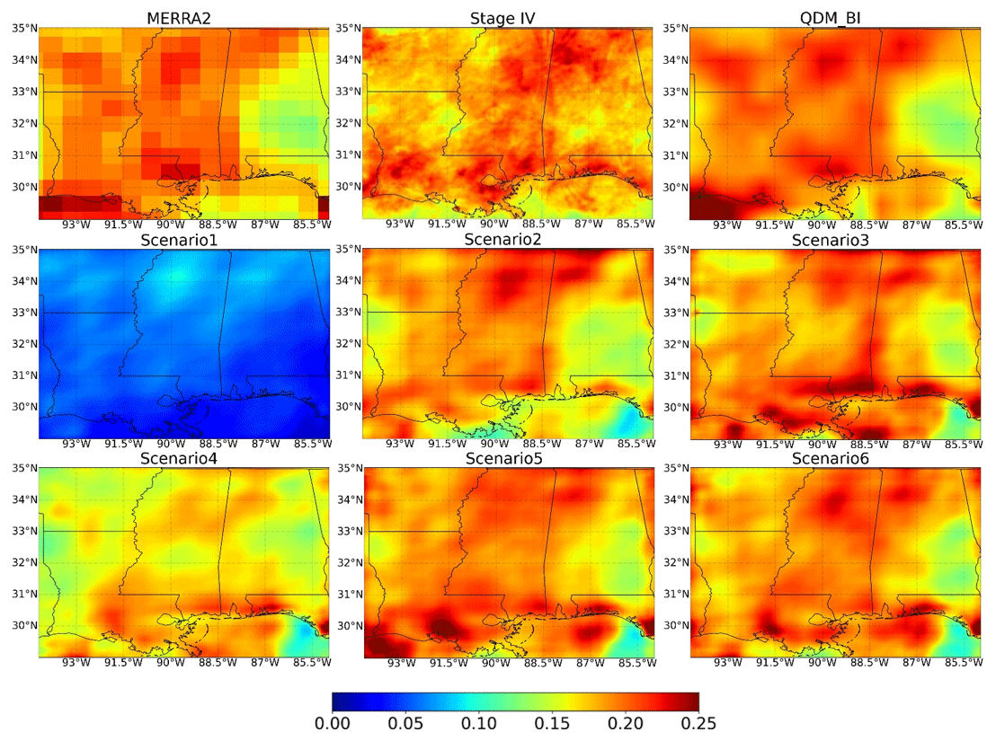
Figure 3 Hourly precipitation climatology (in a unit of mm h⁻¹) during the testing period (2019–2021), which includes MERRA2, Stage IV, QDM_BI, and the six DL experimental runs (Scenario1–Scenario6).

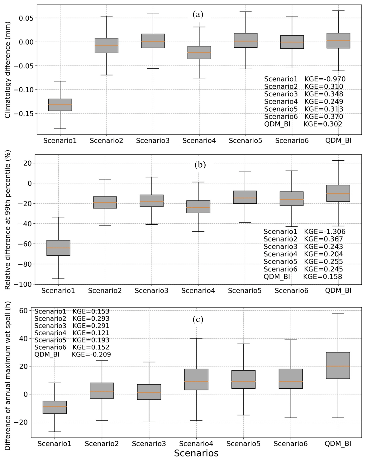
Figure 4 Boxplots showing hourly precipitation estimates minus Stage IV observations based on (a) climatology, (b) extreme at 99 % percentile, and (c) annual maximum wet spell in hours during the testing period (2019–2021). Precipitation estimates are produced from the QDM_BI approach and 6 DL experimental runs (Scenario1–Scenario6).

4.3 Daily and monthly P estimates

We aggregated the hourly P estimates into daily and monthly time scales to evaluate the performance of daily total P and monthly mean of hourly P. Overall, the KGE values for the daily total P are considerably greater than those for the hourly P (Table 3), which suggests that temporal aggregation denoised the hourly precipitation data leading to considerably higher correlation coefficients (r in Table 3), mainly contributing to higher KGE. Similarly, The KGE value for Scenario1 is the lowest as it highly underestimated the mean of daily total P (lower β), overestimated the variability (higher γ), and the correlation r is also lower compared to the other scenarios. Scenario5 and Scenario6 have relatively higher KGE scores than other DL scenarios and QDM_BI for the daily total P. Daily total P from QDM_BI has a comparable KGE score with the DL models while overestimating the variability (higher γ) compared to most of the DL scenarios.

Figure 5 shows the daily total P time series for each year during the testing period for the Stage IV, the 6 DL scenarios, and QDM_BI averaged over the study area. The results show that the daily total P time series from the DL models closely matched with the daily total P time series from Stage IV except Scenario1. Again, Scenario1 highly underestimated the daily total P with the lowest KGE value, suggesting the difficulties of MAE in handling the highly unbalanced feature of P. The daily total P from all the other five DL scenarios is much close to Stage IV with large KGE values (close to or larger than 0.9). Scenario5 and Scenario6 perform better than the other scenarios including QDM_BI, indicating incorporating covariates and corrected coarse resolution P further improved daily total Pestimates. The bias-corrected and downscaled daily total P from QDM_BI, however, highly overestimated the daily total P of Stage IV for almost all the large precipitation events because the bias correction process for QDM_BI was executed individually at each grid cell and did not consider spatial dependencies and nonlinear relationships between covariates and observations, resulting in unstable estimations (Wang and Tian, 2022).

Figure 5 Daily total precipitation during the testing period (2019–2021) from Stage IV, QDM_BI, and the 6 DL experimental runs (Scenario1–Scenario6).

Table 3 also summarizes the statistics of the monthly mean of hourly P. The KGE values for the monthly mean of hourly P are greatly increased, higher than the daily total P. Except for Scenario1, the KGE values for the monthly mean are very close to each other, with Scenario4 slightly lower than others including QDM_BI. The monthly mean from QDM_BI had relatively higher γ, indicating overestimations of variability. Figure 6 presents the monthly mean time series of hourly precipitation for each month during the testing period for Stage IV, the six DL models, and QDM_BI, averaged over the study area. Similar to the daily total P time series, the monthly mean P from all the DL models closely matched with the monthly mean time series from Stage IV (KGE value greater than 0.9) except Scenario1, which highly underestimated the observations. Scenario4 had the lowest KGE value and slightly underestimated the monthly mean, but all the scenarios (Scenario2–Scenario6) are consistently better than the KGE score from QDM_BI. These results indicate that incorporating the weighted loss function (Scenario2–Scenario6 compared to Scenario1) improved monthly mean estimations, and the effects of the other customized components were not obvious at the monthly time scale. Similarly, the monthly mean from QDM_BI estimates has a relatively larger variability than Stage IV, resulting in a lower KGE value.

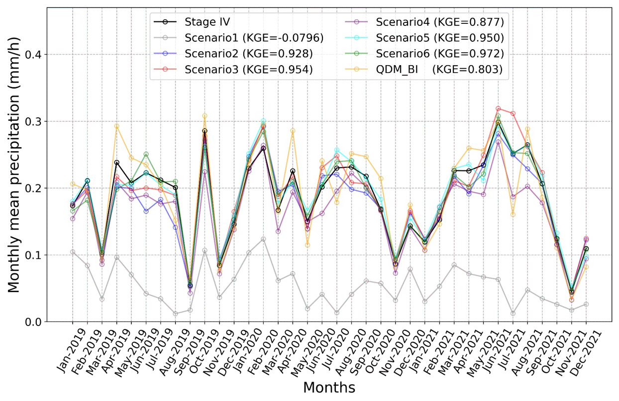
Figure 6 Monthly mean of hourly precipitation time series during the testing period (2019–2021) from Stage IV, QDM_BI, and 6 DL experimental runs (Scenario1–Scenario6).

4.4 Extremes

Table 4 summarizes the statistics of hourly P at the 99th percentile and the annual maximum wet spell. The results show that Scenario1 highly underestimated hourly P at the 99th percentile (lower β than 1) and overestimated variability (higher γ than 1), resulting in a negative KGE score, suggesting the inadequacy of using regular MAE loss function. Scenario2 has the highest KGE score with a higher correlation coefficient (higher r) than the other scenarios. This is probably because the number of trainable parameters for Scenario2 is the lowest, leading to a better regularization ability with limited data for extremes. The KGE values were similar for Scenario3, Scenario5, and Scenario6, and relatively lower for Scenario4, suggesting the importance of incorporating observation-corrected P from coarse resolution as an input. The benchmark approach QDM_BI highly overestimated the variability of hourly P at the 99th percentile compared to Stage IV, resulting in a lower KGE value than most of the DL scenarios except Scenario1. Figure 4b shows the boxplots of the relative difference between hourly P estimates and Stage IV observations at the 99th percentile. On average, Scenario1 underestimated the 99th percentile hourly P by over 60 %, while other DL scenarios underestimated by about 20 %, with Scenario5 and scenerio6 much closer to Stage IV. The 99th percentile estimated by QDM_BI has a much higher variance (as indicated by the distance between high 90 % and low 10 % bars in the boxplot, as well as high γ in Table 4) compared to DL models, while it has a lower mean difference (underestimated by about 10 %) due to bias correction through an explicit adjustment at each percentile. Figure 7 shows the spatial distribution of the hourly P at the 99th percentile for MERRA2, Stage IV, QDM_BI, and the six DL models. We can see that the 99th percentile of MERRA2 hourly P greatly underestimated Stage IV by 40 % (spatial average 2.9 mm for MERRA2 versus 4.8 mm for Stage IV). While the hourly P at the 99th percentile from QDM_BI (area average 4.3 mm) appears to be close to Stage IV, its spatial variability looks very different from Stage IV, probably due to QDM_BI correcting biases on a grid point basis. Scenario4 highly underestimated P values at the 99th percentile compared with other scenarios except Scenario1, indicating that excluding coarse-resolution P as an input is not reasonable.

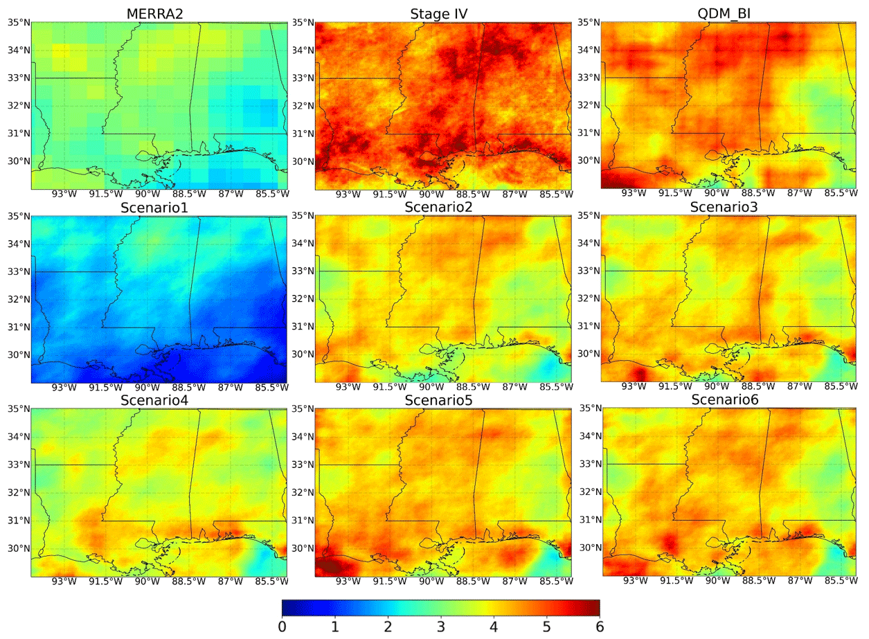
Figure 7 Spatial map of hourly precipitation extremes at the 99th percentile (in a unit of mm h⁻¹) from raw MERRA2, Stage IV, QDM_ BI, and the 6 DL experimental runs (Scenario1–Scenario6).

Table 4 Performance of extreme indices including hourly P at the 99th percentile and annual maximum wet spell in hours. KGE represents the modified Kling-Gupta efficiency (KGE) and it includes three components (correlation component r, bias component β and variability component γ). The correlation component r is represented by the correlation coefficient, the bias component β is represented by the ratio of estimated and observed means, and the variability component γ is represented by the estimated and observed coefficients of variation.

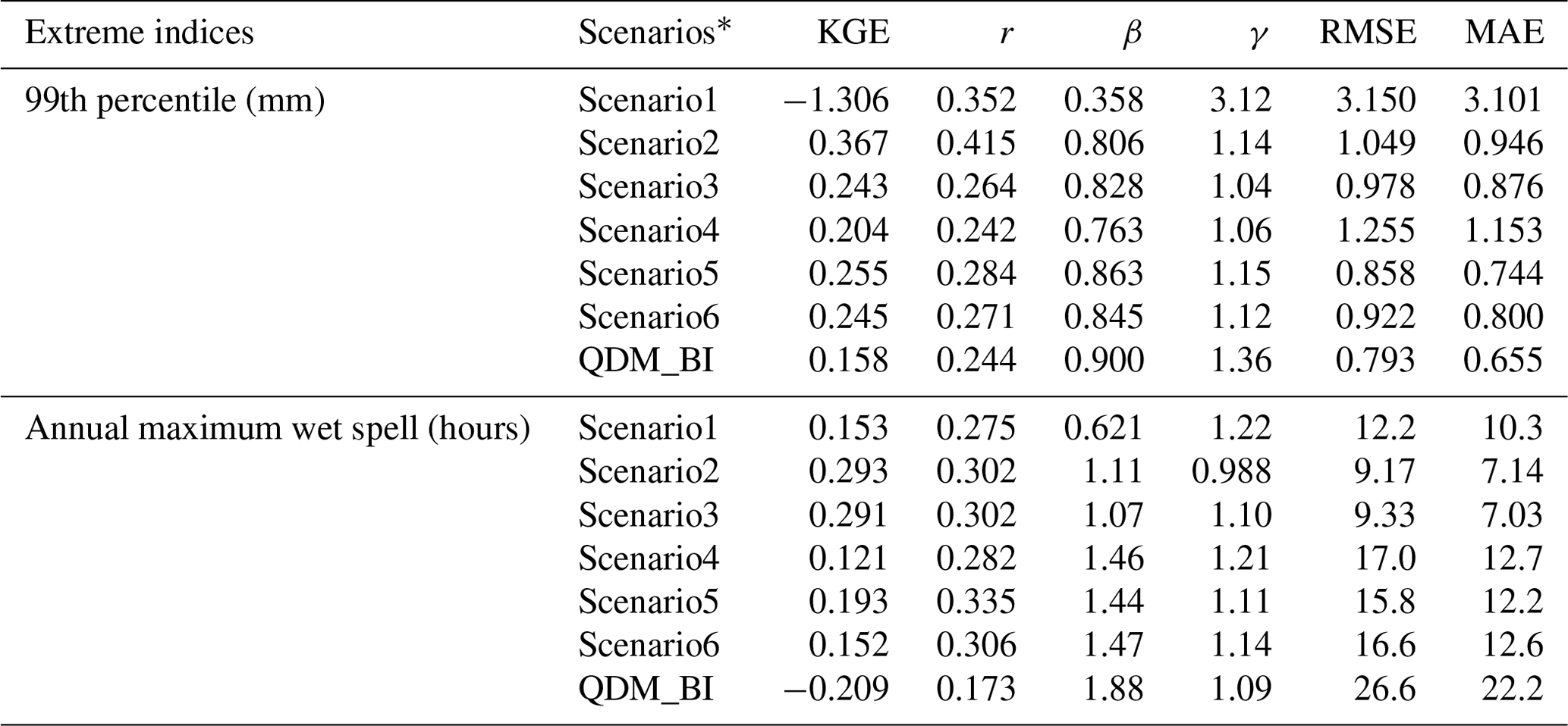
^* Scenarios have different settings: Scenario1 is with a regular MAE loss function and coarse precipitation as a predictor; Scenario2 is with a weighted MAE loss and coarse precipitation as a predictor; Scenario3 is the same as Scenario2 except with a classification as an auxiliary task; Scenario4 is with a weighted loss function and covariates as predictors; Scenario5 is the same as Scenario4 except also including coarse precipitation as predictors; Scenario6 is the same as Scenario5 but including a classification as an auxiliary task.

The DL models treated each hourly P spatial data as a 2D image and did not explicitly account for temporal dependence between images. We assumed that the DL models could potentially preserve the temporal dependence of observations if the DL models well bias corrected and downscaled each 2D image. The annual maximum wet spell is a widely used extreme index for evaluating temporal dependence (e.g., Maraun et al., 2015). The wetness threshold for calculating the annual maximum wet spell index was set to 0.1 mm h⁻¹, which is commonly used for hourly radar data (e.g., Tao et al., 2016). Table 4 shows that Scenario2 and Scenario3 have relatively higher KGE scores for the annual maximum wet spell extreme index than the other DL scenarios, suggesting the usefulness of more parsimonious models with weighted loss function but without including atmospheric covariates as additional inputs. Further incorporating multitask learning (Scenario3 and Scenario6), however, slightly decreased the model performance compared to no multitask learning scenarios (Scenario2 and Scenario5), probably due to the increased parameters and decreased regularization ability. While Scenario1 has the lowest KGE score than the other DL scenarios, it is still much higher than QDM_BI, which highly overestimated the mean of annual maximum wet spell for Stage IV observations (β much higher than 1). Boxplots in Fig. 4c show the difference between model estimates and Stage IV observations for the annual maximum wet spell in hours during the testing period. Scenario1 highly underestimated the annual maximum wet spell by about 10 h. Scenario2 and Scenario3 have the lowest differences with Stage IV in terms of the mean and variance of the annual maximum wet spells. On average, Scenario4, Scenario5, and Scenario6 overestimated the annual maximum wet spell by about 10 h, with Scenario4 and Scenario6 showing a relatively larger variance. The benchmark approach QDM_BI has the largest difference (on average over 22 h) and much larger variance compared to Stage IV, resulting in a negative KGE score. This is probably because QDM_BI corrected biases on a grid basis, which failed to account for the spatial and temporal dependence.

Figure 8 shows an extreme event that occurred from 19:00 to 20:00 on 29 August 2021 in the Universal Time Coordinated (UTC) time zone when Hurricane Ida landed in Louisiana State in the USA from MERRA2, Stage IV, QDM_BI and the six DL scenarios. We can see that MERRA2 highly underestimated this extreme event and did not capture detailed features of Stage IV. While QDM_BI estimates slightly enhanced the hourly P values, they still failed to capture detailed features. Scenario1–Scenario3 gradually enhanced hourly P, but these three models had difficulties capturing the center of the hurricane. By including atmospheric covariates, Scenario4–Scenario6 roughly captured the center of the hurricane, and Scenario6 also reproduced the cyclones surrounding the center. These results suggest that the customized components improve the model performance on bias correcting and downscaling specific extreme events.

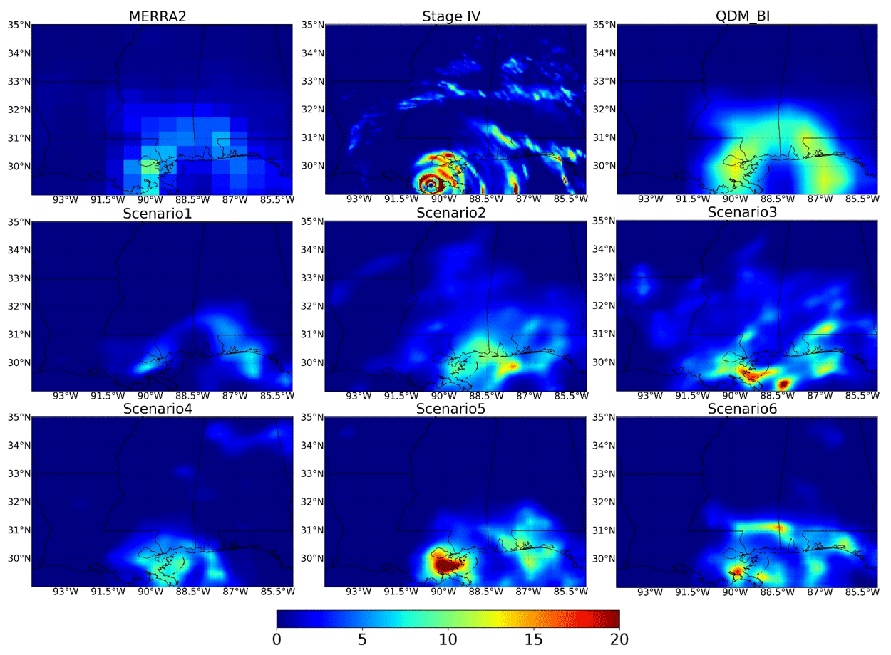
Figure 8 Hourly precipitation (in a unit of mm h⁻¹) from 19:00 to 20:00 on 29 August 2021 in UTC time zone when Hurricane Ida landed in Louisiana, including raw MERRA2, Stage IV, QDM_BI and the 6 DL experimental runs (Scenario1–Scenario6).

4.5 P categories

Table 5 shows that Scenario3 and Scenario6, the scenarios with multitask learning for bias correcting P categories, have larger IOU values (e.g., 19.63 % for Scenario3 and 19.91 % for Scenario6 for moderate rain 2.5–10 mm) than QDM (but 15.30 % for moderate rain) particularly for the three categories with rain, indicating that the two DL models results better matched with the wet categories of the coarsened Stage IV observations than the QDM method. Furthermore, Scenario6 has relatively larger IOU scores than Scenario3, indicating incorporating atmospheric covariates improved the classification accuracy. For example, 8.15 % of the heavy rain category matched the coarsened Stage IV observations for Scenario3, while for Scenario6, 11.07 % of the heavy rain category matched the coarsened Stage IV observations. These results suggest that the auxiliary classification task incorporated in Scenario3 and Scenario6 of the DL model can better estimate the four categories of hourly P during the testing period than the traditional bias correction method QDM.

Table 5 The intersection over union (IOU) comparing coarsened Stage IV with raw MERRA2, QDM and two DL experimental runs with classification task (Scenario3 and Scenario6).

5 Discussion

This study explored customized DL for bias correcting and downscaling hourly P through a set of experiments with or without customized loss functions, multitask learning, and inputs from atmospheric covariates of precipitation. Scenario1, which used regular MAE as a loss function, highly underestimated P for all the temporal scales as well as extremes, showing the lowest performance. As most hourly P are no rain, the regular loss function very likely leads the model to learn no rain events while neglecting rainy events. Regular MAE has been used for downscaling daily precipitation data with limited biases in previous studies (e.g., Sha et al., 2020a), but to our knowledge there are no successful cases using regular MAE for downscaling hourly precipitation data with large biases. However, the scenarios with customized loss functions with weighted MAE (Scenario2–Scenario6) consistently showed much better performance than Scenario1. This result suggests that penalizing more towards heavy P on a grid basis makes the optimization algorithm focus more on the grids where rainfall occurred and, therefore, inherently rebalance the hourly P for model training. While this study explored bias correcting and downscaling hourly precipitation from climate reanalysis data, this algorithm with customized loss function can be potentially integrated with precipitation data from the Global Precipitation Measurement (GPM) mission to generate more accurate operational precipitation data at a finer resolution.

The scenarios with multitask learning indicated limited added values and performed worse than other scenarios without multitask learning in terms of extreme indices. The reason for that is probably because adding multitask learning increased trainable parameters by 30 % while limited extreme data decreased the model regularization ability. Baño-Medina et al. (2020) designed a series of DL models with plain CNN architecture and different model complexity (i.e., increasing the number of trainable model parameters) to downscale the daily ERA5 reanalysis dataset and found that increasing model complexity makes model performance worse, particularly for extreme indices (98th percentile and annual maximum wet spell), which is consistent with our study.

Traditional methods (e.g., QDM_BI) mainly use coarse-resolution P data as the only predictor for downscaling and bias correction, which cannot fully utilize nonlinear relationships between covariates and observations (Rasp and Lerch, 2018) during the bias correction and downscaling process. The DL models with covariates as auxiliary variables, however, have indicated success in improving model performance for postprocessing temperature and precipitation forecasts due to the capability of automatically learning nonlinear relationships between covariates and response variables (Li et al., 2022; Rasp and Lerch, 2018). Scenario4–Scenario6 incorporated physically relevant covariates of precipitation, with only Scenario4 excluding the coarse-resolution P as Baño-Medina et al. (2020) did for downscaling daily precipitation. The results indicate that incorporating auxiliary predictors of atmosphere circulations and moisture conditions can help improve P bias correcting and downscaling skills (see Figs. 3–8). However, only using covariates without coarse-resolution P (Scenario4) is not sufficient to estimate hourly P, while using coarse-resolution P as additional input (Scenario5 and Scenario6) showed improved performance. This result is consistent with a recent study focusing on CNN-based postprocessing of P forecasts from numerical weather prediction models, showing total precipitation itself is the most important predictor (Li et al., 2022). Note that we did not explore the importance of rank among these covariates in improving the model performance in this study, which could be a potential avenue for future work. Furthermore, static variables, such as elevations, long-term climatology (Sha et al., 2020a), soil texture, and land cover, could be helpful for resolving local details. However, our study region has little topographic variations, and therefore including elevation data cannot add any additional information to the model.

Moreover, we compared the customized DL scenarios with the traditional QDM_BI method and found that most of the DL experiments remarkably outperformed QDM_BI in all the temporal scales as well as extremes. The QDM_BI executed bias correction at each grid point without considering spatial dependencies and only used coarse-resolution P as a predictor, and thus does not have the capability of capturing spatial features (e.g., detailed spatial features for the Hurricane Ida in Fig. 8) and accounting for the atmosphere and moisture covariates of precipitation. Furthermore, the proposed customized DL models are fully convolutional, and the trained models can potentially be easily used to estimate hourly P in other places through transfer learning where high-resolution data are not available (e.g., Stage IV radar coverage is limited in the western United States as a result of the scarcity of the radar network and blockage from the mountains, Nelson et al., 2016). There are many questions that need to be explored under this topic about transferability under various climate zones and the impact of spatial distance, which deserves a separate study. The trained models also have the potential to generate high-resolution hourly P estimates beyond the time range covered by Stage IV radars (e.g., before 2002). Furthermore, the SRDRN architecture can be further customized to downscale different gridded precipitation, including downscaling precipitation from GCM projections, which can be a future study.

Due to the stochastic nature of DL models, we ran each DL scenario for three additional times (four times in total) to evaluate the effects of stochasticity compared with the added value of each customized component of DL models (see Tables S2 and S3 in the Supplement). The results show that KGE values for each scenario are significantly different at the p-value of 0.05 at the hourly time scale, which indicates that the added value of each customized component is not caused by model stochasticity. Scenario1 is significantly worse than the other scenarios, including QDM_BI at hourly and aggregated time scales as well as extreme indices, emphasizing the added value of the weighted loss function. Scenario5 and Scenario6 are significantly better than other scenarios, including QDM_BI, in terms of KGE values at hourly and aggregated time scales, and Scenario4 is significantly worse at the monthly time scale. For the 99th percentile extreme index, Scenario4 is significantly worse than Scenario3, sceanrio5, and Scenario6. For the annual maximum wet spell index, Scenario2 and Scenario3 are significantly better than the other scenarios. All these stochastic significance evaluation results are consistent with the findings in Sect. 4. Due to computational requirements (20–22 h for running each scenario once) and resource limits, we ran limited times for each scenario to consider the stochasticity of DL models, and incorporating DL models with Bayesian inference is a potential way to quantify systematic uncertainty caused by the model itself as indicated by Vandal et al. (2018a).

6 Conclusions

Various gridded precipitation (P) data at different spatiotemporal scales have been developed to address the limitations of ground-based P observations. These gridded P data products, however, suffer from systematic biases and spatial resolutions are mostly too coarse to be used in local scale applications. Many studies based on DL approaches have been conducted to bias correct and downscale coarse-resolution P data. However, it is still challenging for traditional approaches as well as current DL approaches to capture small-scale features, especially for P extremes, due to the complexity of P data (e.g., highly unbalanced and skewed), particularly at a fine temporal scale (e.g., hourly). To address these challenges, this study developed customized DL models by incorporating customized loss functions, multitask learning, and physically relevant atmospheric covariates. We designed a set of model scenarios to evaluate the added values of each component of the customized DL models. Our results show that customized loss functions greatly improved model performance compared to the model scenario with regular loss function in all the temporal scales as well as extremes (on average, improved by over 70 % for climatology and over 50 % at the 99th percentile). While multitask learning improved model performance on capturing detailed features of extreme events (e.g., Hurricane Ida), the scenarios with multitask learning performed worse than other scenarios in terms of extreme indices potentially due to the increased number of trainable parameters. The added value of incorporating atmospheric covariates is remarkable, likely because these scenarios took full advantage of nonlinear relationships between large-scale covariates, precipitation, and fine-scale observations. The results also indicated that the role of coarse-resolution P as a predictor is very important for improving model performance despite the added values from the covariates. The DL scenario with customized loss function and coarse-resolution P as the only predictor is the best model at places where no covariate data are available. Moreover, most of the DL scenarios with customized loss functions performed much better in all the temporal scales as well as extremes than the benchmark approach QDM_BI, which is not able to account for spatial dependence and nonlinear relationships. These results highlight the advantages of the customized DL model compared with regular DL models as well as traditional approaches, which provide a promising tool to fundamentally improve precipitation bias correction and downscaling, and better estimate P at high resolutions.