the Creative Commons Attribution 4.0 License.
the Creative Commons Attribution 4.0 License.
 | 05 Sep 2023
Passive-tracer modelling at super-resolution with Weather Research and Forecasting – Advanced Research WRF (WRF-ARW) to assess mass-balance schemes
Yongsheng Chen
Super-resolution atmospheric modelling can be used to interpret and optimize environmental observations during top-down emission rate retrieval campaigns (e.g. aircraft-based) by providing complementary data that closely correspond to real-world atmospheric pollution transport and dispersion conditions. For this work, super-resolution model simulations with large-eddy-simulation sub-grid-scale parameterization were developed and implemented using WRF-ARW (Weather Research and Forecasting - Advanced Research WRF). We demonstrate a series of best practices for improved (realistic) modelling of atmospheric pollutant dispersion at super-resolutions. These include careful considerations for grid quality over complex terrain, sub-grid turbulence parameterization at the scale of large eddies, and ensuring local and global tracer mass conservation. The study objective was to resolve small dynamical processes inclusive of spatio-temporal scales of high-speed (e.g. 100 m s−1) airborne measurements. This was achieved by downscaling of reanalysis data from 31.25 km to 50 m through multi-domain model nesting in the horizontal and grid-refining in the vertical. Further, WRF dynamical-solver source code was modified to simulate the release of passive tracers within the finest-resolution domain. Different meteorological case studies and several tracer source emission scenarios were considered. Model-generated fields were evaluated against observational data (surface monitoring network and aircraft campaign data) and also in terms of tracer mass conservation. Results indicated agreement between modelled and observed values within 5 ∘C for temperature, 1 %–25 % for relative humidity, and 1–2 standard deviations for wind fields. Model performance in terms of (global and local) tracer mass conservation was within 2 % to 5 % of model input emissions. We found that, to ensure mass conservation within the modelling domain, tracers should be released on a regular-resolution grid (vertical and horizontal). Further, using our super-resolution modelling products, we investigated emission rate estimations based on flux calculation and mass-balancing. Our results indicate that retrievals under weak advection conditions (horizontal wind speeds < 5 m s−1) are not reliable due to weak correlation between the source emission rate and the downwind tracer mass flux. In this work we demonstrate the development of accurate super-resolution model simulations useful for planning, interpreting, and optimizing top-down retrievals, and we discuss favourable conditions (e.g. meteorological) for reliable mass-balance emission rate estimations.
- Article
(9582 KB) - Full-text XML
-
Supplement
(8575 KB) - BibTeX
- EndNote


Generating model simulations of atmospheric processes at high spatial and temporal resolutions (super-resolution) has numerous applications, including hybrid physical-model and machine-learning applications (Onishi et al., 2019), dynamic downscaling of coarse-resolution climate and weather information (Watson et al., 2020), and urban-climate feedback studies (Wu et al., 2021). Super-resolution modelling products (e.g. Δx<100 m, Δt<1 s) can also provide desirable information at the scale of measurements during top-down campaigns, which can be analysed in conjunction with measurement data to interpret observations, quantify uncertainty in the measurements, test the validity of assumptions in the employed top-down methodologies, and help fill the information gap in the measurements. In the context of mobile-platform (e.g. aircraft) top-down source emission rate estimations, numerical model simulations can be employed in various approaches. These include offline applications, where a meteorological model (e.g. Weather Research and Forecasting – WRF) is used to replicate conditions during airborne and/or ground-based observations. The model-generated meteorological fields are often used either to drive a separate Lagrangian tracer dispersion model (e.g. HYSPLIT) forward in time to simulate tracer concentrations at observation times and locations or are used for inverse method analysis of emission rates (Cui et al., 2015; Lauvaux et al., 2016; Kia et al., 2022). Previous airborne studies have also used model-generated wind fields and aircraft-measured concentrations for flux calculations and mass-balance analysis (Karion et al., 2015). The emission and transport of passive tracers can be simulated in line with meteorological fields within the same modelling platform, such as the Eulerian WRF model, for source emission characterizations at the scale of observations (Ahmadov et al., 2015; Barkley et al., 2017; Nahian et al., 2020). For these applications, model-generated fields are analysed as complementary information for characterizing emissions based on airborne observational data. For instance, Ražnjević et al. (2022) employed large-eddy-simulation (LES) modelling driven by reanalysis data for interpreting field observations of CH4. Further, model simulations of tracer transport and dispersion have previously been used to assess the uncertainties and errors in top-down retrievals and to optimize the observational approach (Conley et al., 2017; Fathi, 2017; Angevine et al., 2020; Fathi et al., 2021; Fathi, 2022). Numerical model simulations can also be used to simulate ground-based and/or airborne observations, where model-generated fields are used as a proxy for measurement data (virtual sampling). For a robust model-based study of observational methods, model resolutions must be chosen to resolve the timescales and length scales of the measurements. For example, Gasch et al. (2020) simulated aircraft-based Doppler lidar measurements of wind fields through LES modelling at 10 m resolution to investigate airborne lidar measurements for a lidar range length of 72 m.
Fathi et al. (2021) used a regional chemical transport model with physical and chemical process representations (Global Environmental Multiscale - Modelling Air-quality and Chemistry – GEM-MACH) and were successful in evaluating the application of the mass-balance technique in top-down retrievals using model-simulated fields as a proxy for real-world environmental fields. However, the relatively coarse resolution (2.5 km, 2 min) of the employed model was insufficient for the investigation of aircraft-based retrievals through virtual airborne samplings within the model-simulated 4D fields. In airborne campaigns, environmental observations (e.g. wind, temperature, tracer concentrations) are made while flying downwind or around emission sources. These data are then processed through various retrieval algorithms to estimate source emission rates (Peischl et al., 2010; Ryoo et al., 2019; Gordon et al., 2015). Underlying assumptions common among retrieval algorithms are the steady-state conditions during the sampling time of several hours (Alfieri et al., 2010). Data collection during aircraft-based in situ measurements is done through 3D space and over time; thus, (a) any point in space along the flight path is visited only once and (b) spatially adjacent data points are collected at different (consecutive) times. By assuming stationarity (e.g. wind, emissions), the observational data are assumed to be representative of the average conditions during the sampling time. However, time-varying conditions (whether due to turbulence or weather trends) can reduce the representativeness of the sparsely collected environmental data. To study these effects through model simulations, the model resolutions should be chosen to resolve dynamical processes (turbulence) at the spatio-temporal scales at which aircraft in situ measurements are made. For instance, to simulate (and evaluate) in situ measurements at a flying or sampling speed of 100 m s−1 (e.g. onboard instrument sampling frequency ≥1 Hz: Conley et al., 2017; Gordon et al., 2015), the model should be able to simulate (and output) atmospheric fields at length scales and timescales of Δx≤ 100 m and Δt≤ 1 s. Recent real-case LES-modelling studies have commonly referred to such resolutions (Δx≤ 250 m) as “super-resolution” (e.g. Wu et al., 2021; Onishi et al., 2019; Watson et al., 2020). Herein we use the same terminology to describe our WRF model simulations.
The modelling requirements described above motivated the development of super-resolution micro- and LES-scale atmospheric tracer transport model simulations fine enough to resolve smaller-scale flow details and the effects of turbulence and changing stability in atmospheric mixing of tracer concentrations downwind of point and area sources of emission, enabling
-
thorough dynamical evaluation of the application of the divergence theorem and the mass-balance technique in inferring source emission rates;
-
investigation of the effects of flight patterns in aircraft-based top-down retrievals, utilizing a model-generated 4D database;
-
exploration of an improved sampling approach through an optimized flight design and multi-platform (in situ, remote) sampling; and
-
exploration of improved data analysis, post-processing, and interpolation or extrapolation methods needed for flux calculations based on airborne observations.
In this study, we present a proof of concept for performing super-resolution model simulations of atmospheric tracer transport and dispersion using WRF with the ARW (Advanced Research WRF) dynamical-solver core. The concepts that are explored here include (a) realistic modelling of the atmospheric boundary layer at the large-eddy-simulation scale over complex terrain, (b) mass-conserved modelling of atmospheric dispersion and transport of passive tracers under the conditions described in (a), and (c) generation of modelling products at the spatio-temporal scale of airborne observations (aircraft-based in situ and remote measurements) that are useful for evaluating the observational methods and providing recommendations for future studies. We evaluate the performance of our model simulations against historical observational data from ground-based monitoring stations and aircraft-based observations from a 2013 airborne campaign, the Joint Canada-Alberta Implementation Plan on Oil Sands Monitoring (JOSM, 2013). We further assess the performance of our simulations in terms of global (over the entire modelling domain) and local (sub-domain) mass conservation by conducting 4D mass-balance analysis.
We explore three different cases (dates and times) during August and September 2013 over Canadian oil sands (Athabasca, Alberta). We use reanalysis data as initial and boundary conditions for our case studies. To achieve the desired micro- and LES-scale resolutions, we perform multi-domain nested simulations with LES parameterization for the finest domains. Further, we modify the WRF source code (dynamical solver) to simulate the release of passive tracers from point and area sources within the finest model domain. The novel modelling approach with WRF presented in this work is comprised of (1) dynamical downscaling of reanalysis data from synoptic to LES resolution, (2) super-resolution model simulations through horizontal nesting and vertical grid refining, (3) LES sub-grid parameterization, and (4) passive-tracer transport and dispersion simulations. To the best of our knowledge, the combination of these capabilities in WRF modelling has not been explored extensively in the past where reanalysis-driven super-resolution dispersion modelling under local mass-conservation conditions is conducted. In this work we discuss a series of modelling best practices for such simulations in the context of our case studies, for improved modelling of atmospheric pollutant dispersion. The modelling approach in this work is geared towards the assessment of mass-balance methodologies, but throughout we discuss the general usefulness of super-resolution modelling for generating highly resolved (spatial and temporal) pollutant dispersion forecasts and their potential application in measurement planning and interpreting the observations. The model output data from the super-resolution simulations in this work are also used to evaluate the accuracy of aircraft-based emission rate retrieval methodologies in Fathi (2022).
2.1 Case studies
For this work we chose our case studies from the times and locations of three emission estimation flights during the JOSM 2013 campaign over the Athabasca oil sands region (Alberta, Canada). This choice was made to enable qualitative comparisons to observations. We considered the geographical location of an oil sands facility, Canadian Natural Resources Ltd. (CNRL). We configured our WRF model domain centred over the CNRL facility. For our WRF simulations, we considered model simulation times overlapping those of three JOSM 2013 box flights over CNRL (see Table 1). “Box flight” refers to closed-shape (e.g. rectangular, cylindrical) flight paths around the target emission source, where aircraft-based measurements are used to estimate source emission rates using the mass-balance technique (Gordon et al., 2015). Note that case 2 on 26 August 2013 was a “rejected” case in the actual campaign analysis due to unsuitable atmospheric conditions for aircraft-based retrievals (Fathi et al., 2021), but it is analysed here as an assessment of the super-resolution model.
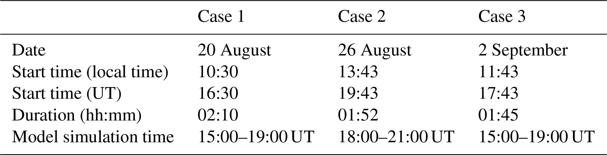
Table 1Three case studies during late August and early September of 2013 over the CNRL oil sands facility. Times and locations for the case studies were chosen from three JOSM 2013 box flights.
For each of these three cases, 11 tracer emission scenarios or sources are considered. Table 2 provides the spatial details for the different emission sources, including seven elevated point sources (representing stack emissions), two small-area sources (representing surface mines), a large-area source (representing the tailing pond west of CNRL), and a long multi-section line source (over the approximate extent of the Horizon Highway south of CNRL). Table 2 lists geographical coordinates and tracer release heights (e.g. stack top height) for all of the sources. Horizontal dimensions are also provided (in brackets) for the line and area sources. The horizontal dimensions for each of the point sources are equal to those of one grid cell in the finest model domain. Coordinates and heights for CNRL1–4 correspond to actual (real-world) stacks in the CNRL facility. The hypothetical source (CNRL0) is co-located with CNRL1 and CNRL4, with the stack top or release height over 4 times higher than the tallest facility stack (CNRL1), simulating the initial (assumed instantaneous) plume rise due to buoyancy. Figure 1 shows a map of the region with the location and spatial extent of case study emission sources marked (labelled) in red. The large rectangular area (surface) source represents the tailing pond to the west of the CNRL complex. The multi-segment line (surface) source represents the Horizon Highway south of CNRL. Two small-area sources labelled MINE1 and MINE2 represent emissions from surface mine excavation sites within the CNRL complex. Figure 1 also shows the locations of two hypothetical point (stack) sources: CNRLs (south) and CNRLw (west). During two of our case studies on 20 August 2013 (case 1) and 2 September 2013 (case 3), the mean wind was from the west and south-west, placing these two hypothetical stacks upwind of the CNRL facility.
Table 2Eleven tracer emission scenarios, including seven point sources representing release from stack tops at various heights, three area sources including a large-area tailing pond towards the western side of the facility and two smaller (in area) surface mines, and a line source approximately spanning the extent of the Horizon Highway south of the facility. Note that heights and locations for sources with superscript * are hypothetical.
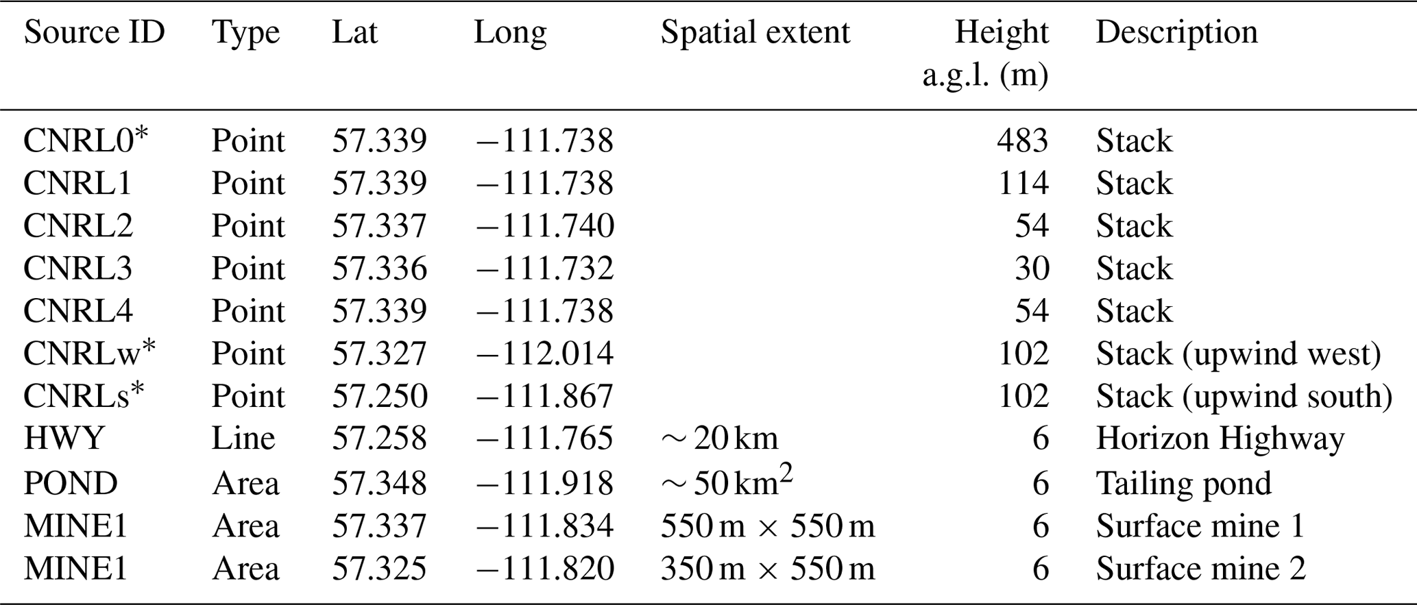
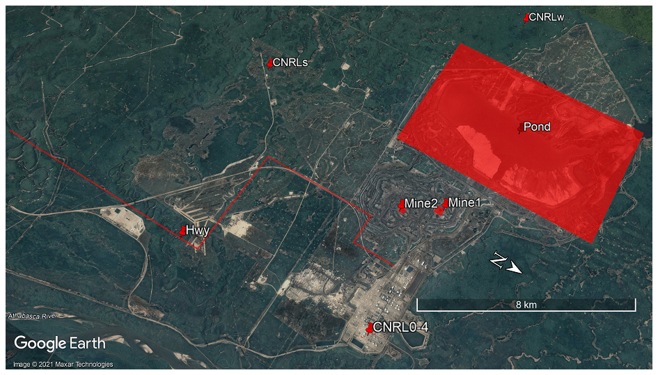
Figure 1© Google map (2021) of the study region. The CNRL oil sands facility with case study emission sources is marked on the map, including seven point sources, two area sources, a large-area surface source (tailing pond), and a multi-segment line source (road or highway). Direction north (N) is shown with a compass arrow.
2.2 Model and technical set-up
For this work, the Weather Research and Forecasting (WRF version 3.9, https://www2.mmm.ucar.edu/wrf/users/download/get_source.html, last access: 4 July 2023, Skamarock et al., 2008) model with the ARW dynamical core was utilized. WRF-ARW provides a multi-scale simulation framework suitable for efficient parallel computing with a vast range of physical parameterizations adaptable for different scales and dynamical processes. The Advanced Research WRF (ARW) solver features a suite of fully compressible Euler non-hydrostatic equations for solving prognostic variables, including velocity components in Cartesian coordinates (u, v, w), and scalars such as water-vapour mixing ratio and tracer concentration. The third-order Runge–Kutta scheme (RK3) is used for time integration in ARW (Wicker and Skamarock, 2002). The spatial discretization in WRF-ARW uses Arakawa C-grid staggering with thermodynamics (scalar) variables (e.g. moisture, tracer) defined on grid cell centres (mass points) and velocity components defined normal to the respective faces of model grid cells (one-half grid length from mass points). Second- to sixth-order spatial discretization and the RK3 time-integration scheme are available in ARW to solve for advection of momentum, scalars, and geopotential in flux form (the governing equations). The RK3 transport–advection (combined with flux divergence) in WRF-ARW is conservative; however, it does not guarantee positive definiteness on its own. Negative mass creation is offset by positive mass such that tracer or scalar mass is conserved over the modelling domain (Skamarock et al., 2008). Negative mass can be set to zero, but this will result in an erroneous increase in tracer mass within the modelling domain. By choosing a positive-definite scalar advection option in WRF-ARW, as we did in our simulations, a flux re-normalization is applied to the transport step to remove the non-physical effects such as creation of the negative mass (Skamarock and Weisman, 2009). To summarize, if the outgoing fluxes (removing mass from the control volume) in the final step of RK3 predict a negative updated scalar or tracer mixing ratio, the outgoing fluxes are re-normalized to be equivalent to mass within the volume. For more details, see Sect. 3.2.3 in Skamarock et al. (2008). Various formulations are available in the ARW solver for explicit spatial diffusion (turbulent mixing), including a sixth-order spatial filter proposed by Xue (2000). The implementation of this scheme in ARW is described in Knievel et al. (2007). The sixth-order turbulent diffusion scheme is also prone to creating negative mass due to negative up-gradient diffusion. Monotonicity can be enforced in the model (user-specified option) by setting negative diffusive fluxes to zero; however, it does not conserve scalar mass (Skamarock et al., 2008). Hence, in our simulations we used the sixth-order diffusion scheme without the monotonic option.
Mesh refining and increased resolution can be achieved in WRF through series or concurrent grid nesting in the horizontal dimensions. With concurrent grid nesting, multiple computational domains with increasing resolution can be integrated simultaneously. The process where the coarse “parent” domain's output is interpolated to provide initial and lateral boundary conditions for the fine “child” domain is referred to as one-way nesting. Two-way nesting is achieved when information from the child domain is aggregated to write the overlapping regions of the parent domain. At high resolutions (<3 km), mesh refining in WRF via grid nesting only in the horizontal dimensions limits control over the grid aspect ratio, which can lead to poor grid quality and numerical errors. It has been shown that grid quality affects the accuracy of numerical solutions (Lee and Tsuei, 1992; You et al., 2006). A procedure permitting vertical nesting for one-way concurrent simulation is developed and described in Daniels et al. (2016) and allows high resolutions of the order of metres, while grid quality is maintained. This procedure permits one-way concurrent grid nesting in both the horizontal and vertical, and this is utilized here for WRF simulations with five domains (d01–d05) with increasing resolutions from ∼31 km to 50 m in the horizontal dimensions and up to a near-surface vertical resolution of ∼10 m in the finest domain (d05).
With regards to nesting in the horizontal, Skamarock et al. (2008) recommended the use of odd nesting ratios such as 1:3 and 1:5 (as opposed to even ratios like 1:2) due to the staggered structure of the Arakawa C grid used in the WRF-ARW modelling framework. Mohan and Sati (2016) investigated the impact of different nesting ratios in WRF and found no statistically significant difference in simulated results with ratios 1:3, 1:5, and 1:7, suggesting that larger ratios can be used to reduce the computational cost in nested simulations. However, larger ratios (e.g. 1:9) can result in increased interpolation errors and are not recommended. In this work, as a compromise between numerical accuracy and computational cost, we used a 1:5 nesting ratio. Figure 2a shows the five domains of the model and their relative sizes. Model domains are centred on the region of Athabasca oil sands, with the two finest domains (d04 and d05) centred on the CNRL Horizon facility in the north-western quarter of the complex, west of the Athabasca River. Figure 2b shows a map of the region with the CNRL facility marked on the map (red star). Boundaries of the two finest domains, d04 and d05, are also overlaid on the map in Fig. 2b. The relative location of the other oil sands facilities can be seen in the figure. CNRL is in the north-western corner of the complex, with no facilities to its north and west. The oil sands region is located in the Athabasca River valley, with 400–500 m vertical relief within a few tens of kilometres of the facilities (mainly in the west–east direction). This may give rise to complex flow conditions and frequent vertical wind shear in the valley (Gordon et al., 2018). In Sect. 3.2 we discuss the performance of our super-resolution model simulations against the observed meteorology for the same locations and time periods.
The North American Regional Reanalysis (NARR) GRIB (GRIdded Binary) data (at 3 h intervals) from NOAA (National Oceanic and Atmospheric Administration) archives were used for August and September 2013 (the period of the JOSM 2013 campaign) over the Athabasca oil sands region (Alberta, Canada). The NARR data used for this study can be accessed at NOAA-Fathi (2022). Realistic WRF-ARW simulations were carried out with concurrent one-way grid nesting in the horizontal dimensions with five domains (d01–d05) at a ratio of 1:5 and with mesh grid refining in the vertical for the two smallest and finest domains (d04 and d05) by consecutively increasing the number of vertical levels near the surface. The finest domain (d05) has a horizontal grid size of Δx=50 m over the entire domain, a Δt=0.16 s model simulation time step, and Δz=11.62 m for the first 40 full grid levels near the surface. Note that the vertical resolution of about 12 m for the bottom 500 m a.g.l. (above ground level) is sufficient for investigating and evaluating different methods for extrapolating sampled data below the lowest flight level (typically ∼ 150 m) where no aircraft measurements are usually made, which is required for flux estimations in top-down emission rate retrieval methods (Gordon et al., 2015). Further, note that Δx and Δt configurations are set as such to ensure the Courant–Friedrichs–Lewy (CFL) stability criterion , where is the maximum wind speed in the model (Jacobson, 2005). Table 3 provides the details of model grid configurations for the five domains.
Table 3Case study model set-up for model simulations with five domains with increasing resolution. The first three domains have the same coarse vertical grid. Domains d04 and d05 have increasing resolution via vertical grid refining. The finest domain (d05) has Δz≃12 m for the first 40 levels near the surface. Δx and Δt indicate the horizontal grid size and the model simulation time step, respectively, for each domain. X and Y indicate the domain dimensions. nx, ny, and nz are the number of computational grid points in each direction, with the model's top layer at 15.623 km (15.350 km a.g.l.) and the pressure level 10 kPa for all the domains.
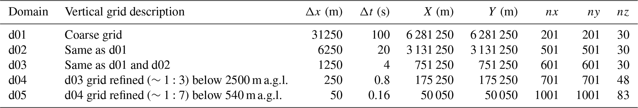
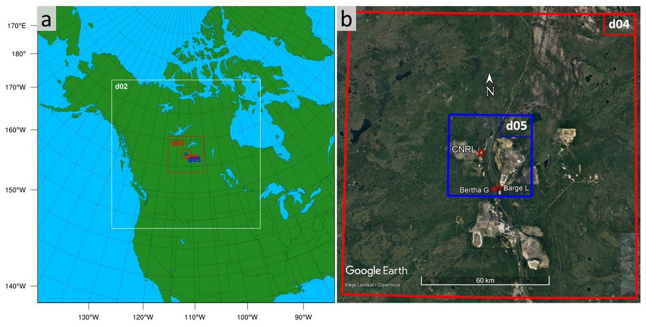
Figure 2(a) WRF model grid (horizontal) configuration with five nests d01–d05 with increasing resolution (decreasing domain size) at a ratio of 1 to 5. The finest domain, d05, is centred over the oil sands region. (b) © Google map (2021) of the oil sands region with an overlay of model domains d04 and d05. The CNRL facility is marked with a red star. Locations for two WBEA monitoring stations are also shown with red triangles: Bertha Ganter–Fort McKay and Barge Landing monitoring stations.
In order to simulate small-scale atmospheric dynamical processes, the finest two model domains (d04 and d05) were configured with the following diffusion scheme and LES sub-grid parameterization options available in the WRF model (Skamarock et al., 2008).
-
The diffusion option was set to “full-diffusion” mode (diff_opt=2) to accurately compute horizontal gradients using full metric terms.
-
The horizontal diffusion option was configured with the sixth-order diffusion scheme (diff_6th_opt=1).
-
For vertical and horizontal diffusion by sub-grid turbulence, the “K option” was set to km_opt=2 to solve a prognostic equation for turbulent kinetic energy (TKE) where the diffusion coefficient K is calculated based on TKE (see Appendix A).
WRF 3.7+ includes a basic framework for initiating and creating continuous (and variable) emission tracer plumes. To simulate the emission of passive tracers, the WRF dynamical-solver source code was modified following an approach similar to Blaylock's (as described in Blaylock, 2017) and used in Blaylock et al. (2017). Tracer amounts were initiated at several different horizontal locations within the finest domain (d05) after 30 min of model simulation. A meteorological spin-up time of 1 h was considered through testing with the modelling set-up for different initial and boundary conditions according to the following criteria. For the cases we considered, within the first hour of simulation time, (a) the model boundary conditions propagated over the entire span of domain d05, (b) model winds (in the west–east and south–north directions) assumed continuous profiles both horizontally and between model vertical layers, and (c) water vapour on model mass layers (horizontal and vertical mass grid points) assumed continuous profiles within this time period. Tracer release for our considered emission scenarios (see Table 2) started after a 30 min spin-up time (half the meteorological spin-up time) and continued for the rest of the simulation period. These included surface emissions on several model grid points at the lowest level (i.e. level 1 at ∼ 6 m a.g.l.) at various locations and stack emissions at levels 3, 5, 9, 10, and 40 according to the stack top heights and horizontal locations described in Table 2. Note that, in WRF-ARW, vertical levels (Fig. S1) are configured using a terrain-following hydrostatic-pressure coordinate system (Skamarock et al., 2008), and therefore stack top heights for our simulations are assigned to pressure levels with heights (in metres) closest to the source heights. Depending on pressure changes, the heights of pressure levels can vary over time. This variation was determined to be smaller than the corresponding vertical level thickness for our simulations, and therefore its impact on tracer release simulation is considered negligible in this work. All of the tracer emissions were implemented within the boundaries of the CNRL facility and the surrounding region in the eastern half of the modelling domain. All the emission scenarios involved the emission of passive and non-buoyant tracers with no interactions with meteorology and no defined surface deposition rates. Note that the topography input information (land use indices) used in our WRF simulations was not modified to represent oil sands operations (e.g. tailing ponds, excavation sites) and only represents natural features (e.g. river basins, hills). The release, dispersion, and transport of tracers from our emission scenarios under different meteorological conditions are discussed in Sect. 3.3.
2.3 Divergence theorem and the mass-balance technique
For this work, the mass-balance technique is utilized for calculating the net integrated flux out of virtual control volumes (emission box) enclosing the emission sources of interest. The calculation steps in this section follow those in Fathi et al. (2021), with slight modifications for use with WRF model output data. For a detailed discussion on the application of the mass-balance and divergence theorem in estimating source emission rates, see Fathi et al. (2021).
In applying the mass-balance technique to estimate the rate of emissions from sources within a flux box (control volume), the mass flux exiting the box through the box top and lateral walls is equated to the emission rate of the tracer within the box. The processes contributing to the change of mass, for a passive tracer, within the control volume can be described with the following expression:
where the storage term SC represents the change in mass of tracer C within the control volume, EC represents the tracer emission rate, and FC,H and FC,V represent the net horizontal and vertical advective fluxes exiting through the lateral and top walls, respectively, of the flux box. FC,HT and FC,VT represent horizontal and vertical turbulent fluxes, respectively, across the box walls.
The total mass of the tracer within the control volume can be calculated by integrating the mass over the entire volume of the box at each model output time stamp (Δt=1 s):
where is the tracer concentration at each model grid point. Further, the storage term can be calculated by taking the time derivative of BC,Tot(t):
Horizontal advective flux through the lateral walls of the box can be calculated by extracting tracer concentration and normal wind (positive outwards) along the lateral walls of the box from model output:
where ds(x,y) is the path s(x,y) increment along the walls. U⊥ is the normal wind to the box walls (positive outwards).
Similarly, the vertical flux through the box top can be calculated as
where and are the tracer concentration and vertical wind speed, respectively, at the box top. See Appendix B for turbulent flux terms. As we show later, the vertical advective (FC,V) and turbulent (FC,HT, FC,VT) fluxes have negligible relative contributions to the mass-balance equation, with the horizontal advective flux FC,H being the dominant term removing mass from the box. We collect all the flux terms (advective and turbulent) contributing to the removal of tracer mass from the box into a single flux-out term as . By rearranging Eq. (1), the tracer emission rate can be estimated based on the other terms as
By extracting the required fields from the model output 4D database, Eq. (6) can be utilized to determine the source emission rate based on the mass-balance equation, which can then be compared to the known input emission rate. Following the calculation process described above, source emission rates can be estimated at each model output time step and compared to the model input emissions to evaluate model performance in terms of local mass-conservation and mass-flux consistency. See Table S1 for discrete integral expressions of different terms in the mass-balance equation (Eq. 6). Note that, for flux calculations in this work, model wind fields were linearly interpolated onto the mass grid points (where concentration fields are defined).
Model simulations were carried out for the period between 15:00 and 19:00 UT for cases 1 and 3 on 20 August and 2 September 2013, respectively. The simulation period for case 2 on 26 August 2013 was between 18:00 and 21:00 UT (see Table 1). NARR data at 31.25 km resolution were used as initial and boundary conditions for the coarsest domain (d01) with the same resolution. Through model nesting at an increasing resolution (and decreasing size) ratio of 1:5, the input reanalysis data were downscaled to consecutively higher resolutions all the way to 50 m in the finest domain (d05). Each parent domain provided initial and boundary conditions for their nested child domain: d01 ⇒ d02 ⇒ d03 ⇒ d04 ⇒ d05. Note that feedback (two-way nesting) between the parent and nested domains was turned off to allow for vertical grid refining for domains d04 and d05. Output frequency was set to 3 h for domains d01–d03, 100 s for d04, and 1 s for d05.
3.1 Model sensitivity
Sensitivity analysis showed consistent performance by the five nested domains. For instance, output from the three finest domains (d03, d04, d05) for case 1 agreed to a great extent for sea level pressure, with <1 hPa difference, relative humidity (at 2 m a.g.l.) with 2 % difference, and temperature (at 2 m a.g.l.) within 2–3 ∘C. Wind directions were also consistent with a 2–7∘ difference for a mean wind direction from about 240∘ (west–south-west). Wind speeds were biased high relative to domain d03 with a mean wind speed of about 6 m s−1, by 0.7 to 1.5 m s−1 for domain d04, and by 3 to 4 m s−1 for domain d05 (see Fig. S2 in the Supplement for a comparison of wind vertical profiles from these three domains at 18:00 UTC).
Table 4Comparison of domain d05 simulations against d04 output fields every 100 s at the geographical location of the CNRL oil sands facility (lat =57.339∘ N, long .738∘ W). Note that positive and negative signs indicate overestimates and underestimates by d05 relative to d04.
We also compared the d04 and d05 simulations to d03 at the geographical location of CNRL. The comparison was made in terms of easterly (U) and northerly (V) wind components, 2 m temperature, 2 m relative humidity, and sea level pressure (SLP) (see Fig. S3 for case 1). Root mean square (rms) differences were small (e.g. 0.5 m s−1 for U, 0.68 m s−1 for V, and 0.45 ∘C for temperature) for d04 simulations at 250 m horizontal resolution and with LES parameterization. The rms differences for d05 simulations were also similarly low for SLP, temperature, and humidity, with wind speed biased high by 1.57 and 3.47 m s−1 for V and U, respectively (at 10 m a.g.l.). As the model output data from domain d03 were only for every 3 h, to evaluate the performance of domain d05 simulations at CNRL at a higher temporal resolution, we performed evaluations against domain d04 with model output every 100 s. Evaluation results for all three cases are summarized in Table 4. The rms difference ranges from 0.09 to 0.56 hPa for SLP, from 1.89 % to 7.59 % for 2 m relative humidity (RH), from 0.25 to 1.84 ∘C for 2 m temperature, from 0.59 to 3.16 m s−1 for the west–east wind component U, and from 0.75 to 2.20 m s−1 for the south–north wind component. For case 1 on 20 August 2013, 2 m temperatures ranged from 17 to 20 ∘C and 10 m wind speeds from 6.6 to 11.4 m s−1 at the geographical locations of the main CNRL stack sources. For case 2 on 26 August 2013, the 2 m temperature range was similar to case 1, but the 10 m wind speeds were much lower, ranging from 0.8 to 3.5 m s−1 with a mean of 2.8 m s−1. For case 3 on 2 September 2013, 10 m wind speed ranged from 5.3 to 9.4 m s−1 with 2 m temperatures slightly higher than the other cases, ranging from 21 to 23 ∘C. The temperature and wind speed ranges mentioned for the three cases are for periods between 18:00 and 20:00 UT (local noon to 14:00).
3.2 Meteorological evaluation
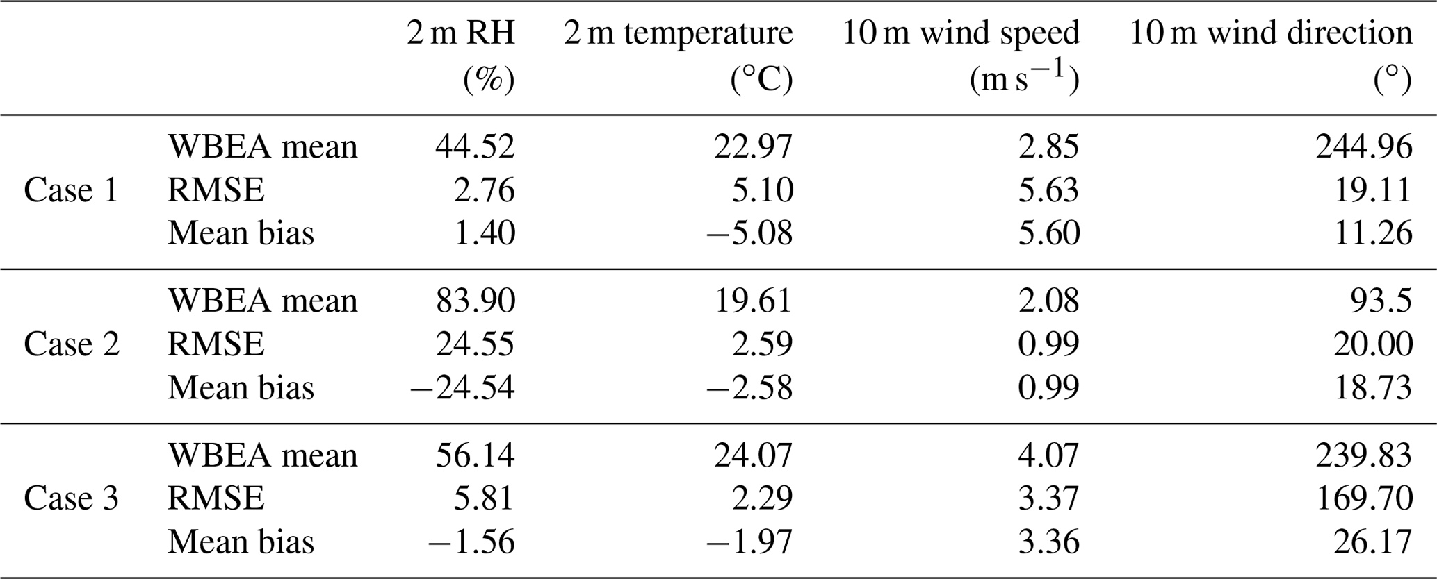
Output from the three finest domains was compared to the concurrent historical observational data from the Wood Buffalo Environmental Association (WBEA) continuous monitoring stations Bertha Ganter–Fort McKay and Barge Landing for the periods of interest in August and September 2013 (https://wbea.org/data/continuous-monitoring-data/, last access: 4 July 2023). The WBEA data used in this study can be accessed at WBEA-Fathi (2022). See Fig. 2b for the locations of the two WBEA stations on the map of the region (red triangles). We compared model 2 m relative humidity, 2 m temperature, and 10 m wind to the corresponding WBEA observational data. Model values at 2 m for domains d03–d05 and at 10 m for domains d03 and d04 were output by WRF as diagnostic variables. Model winds at 10 m a.g.l. for domain d05 were determined by linearly interpolating between model grid point values at the surface and at the top of the first model layer at ∼ 12 m a.g.l. Figure 3 shows wind-rose diagrams for case 1 on 20 August, where output from model domains d03, d04, and d05 is compared to WBEA data at the location of Bertha Ganter–Fort McKay monitoring station. Wind directions for this case were from west and west–south-west during the simulation time, which is consistent with the observed WBEA wind directions. Model wind directions were within 20 to 30∘ of the WBEA observational data. Model wind speeds were higher for all three domains compared to WBEA observational data for the locations of the two monitoring stations (with a mean wind speed of 2.85 m s−1): by 2–3 m s−1 for domain d03, by 3–4 m s−1 for domain d04, and by 4–6 m s−1 for domain d05. Note that the LES sub-grid parameterization was used for the d04 and d05 simulations. Model winds for these two domains, especially for d05, were highly variable over time and space. Figure 4 shows output from d04 and d05 compared to observational data from the two WBEA monitoring stations for 10 m wind, 2 m temperature, and 2 m relative humidity for case 1. Comparisons for the other cases show similar results, with agreements within 5 ∘C for 2 m temperature, 1 %–25 % for 2 m relative humidity, and 20–30∘ for wind direction. Similarly to case 1, wind speeds were higher than WBEA winds by between 3 and 6 m s−1 for case 3. Model wind speeds for case 2 were less than 1 m s−1 higher than WBEA observations, with an average wind speed of 2.08 m s−1. Evaluations for domain d05 against WBEA station Bertha Ganter–Fort McKay (AMS01) are summarized in Table 5 .
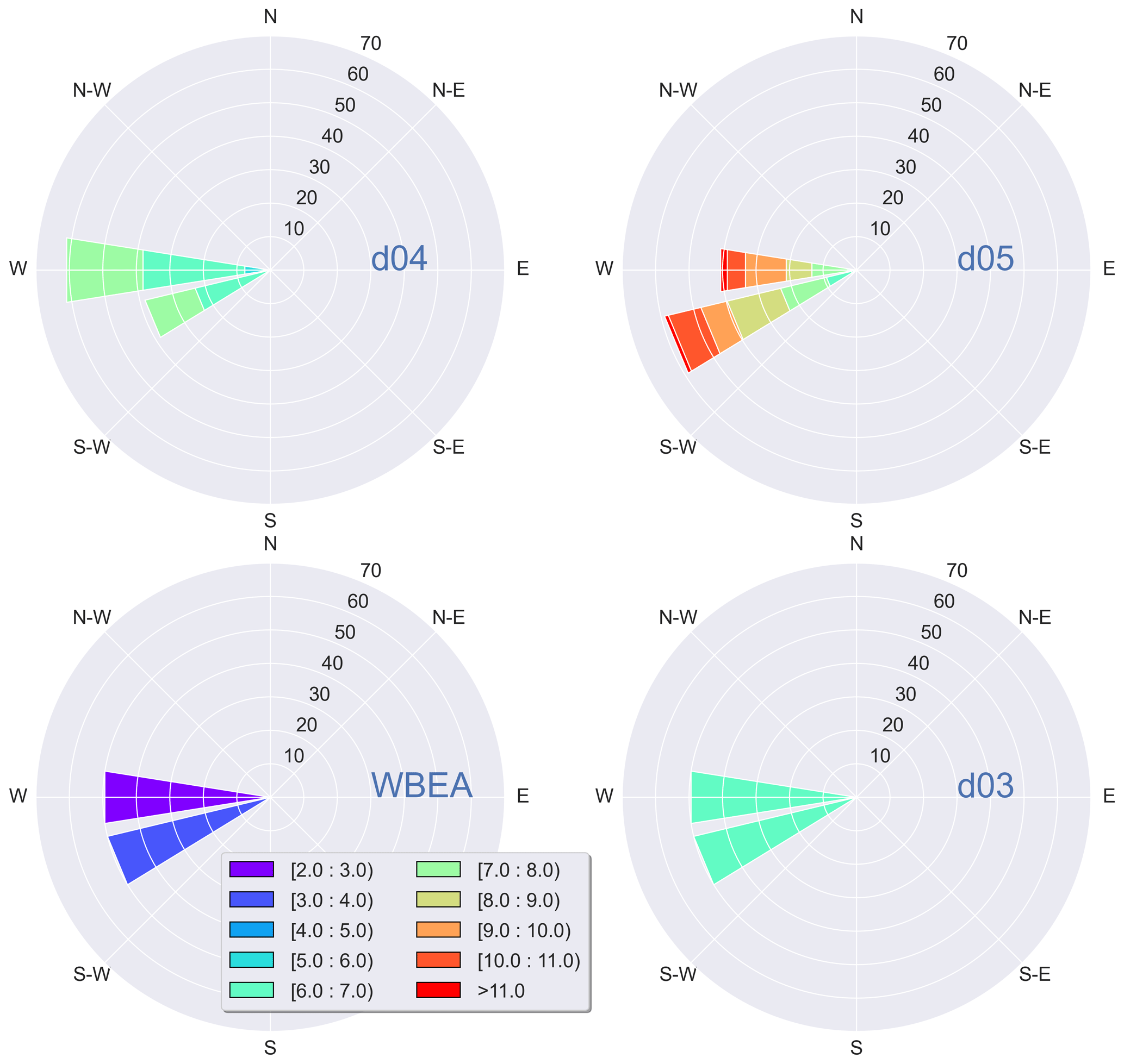
Figure 3Wind-rose diagrams comparing observational data from WBEA monitoring station Bertha Ganter–Fort McKay to model output (case 1) winds at the location of the WBEA station from domains d03, d04, and d05 for 20 August 2013. Wind distributions, indicated in each circle, are in units of percentage. Wind directions are consistent within 20∘, blowing from W-SW towards E-NE.
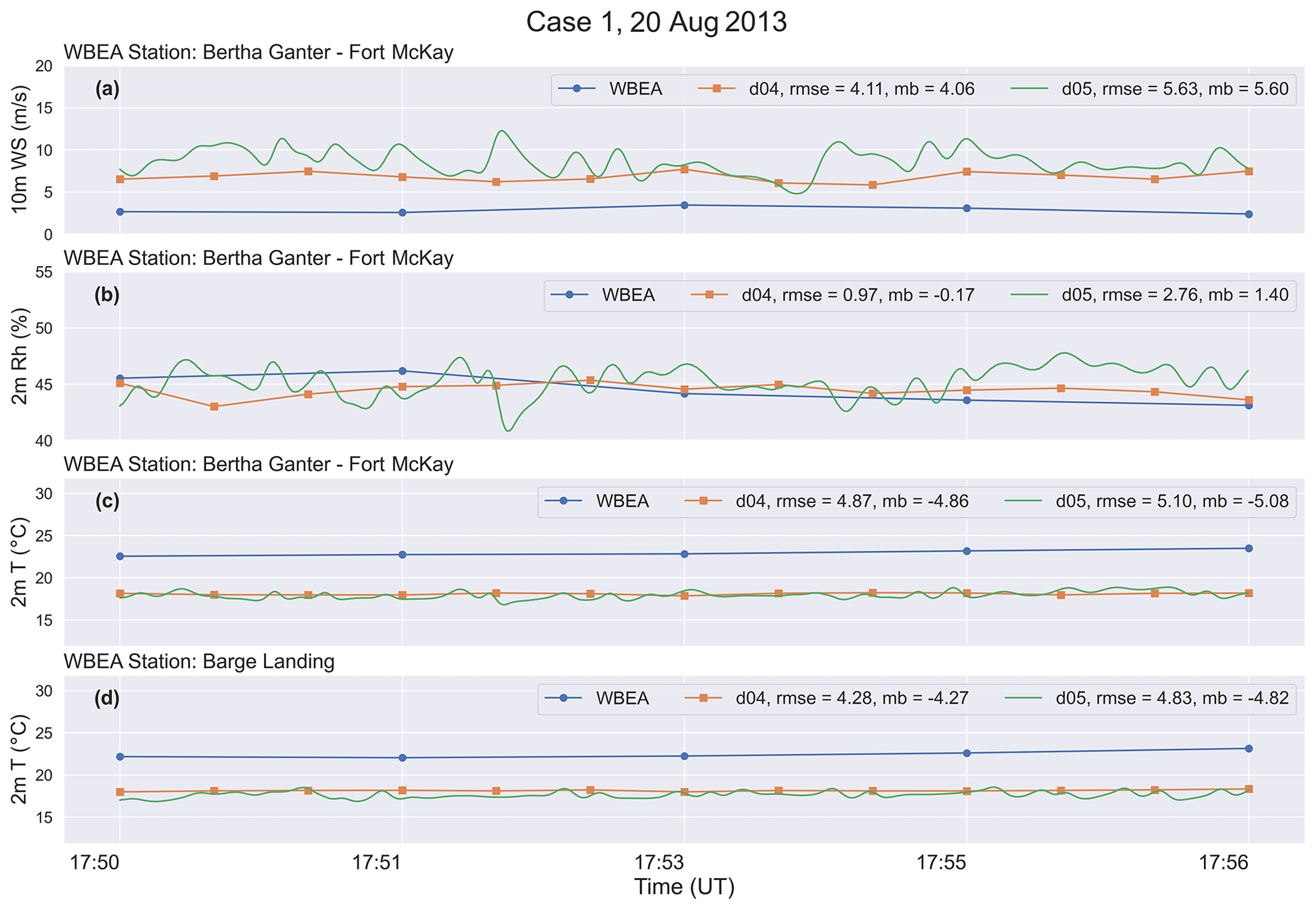
Figure 4Case 1 model output from domains d04 and d05 for (a) 10 m wind speed, (b) 2 m relative humidity, and (c, d) 2 m temperature is evaluated against observational data from WBEA monitoring stations in terms of RMSE and mean bias (mb).
Table 5Meteorological evaluation of domain d05 simulations against WBEA observational data at the geographical location of Bertha Ganter–Fort McKay (AMS01) station. Model performance is shown in terms of root mean square (rms) difference and mean bias. Positive and negative values indicate overestimates and underestimates by d05 relative to WBEA-AMS01 observations.
We note the following considerations when comparing model-generated fields (e.g. wind) to WBEA observational data.
-
The lack of observational data from continuous monitoring stations for more spatial locations, especially closer to the centre of domain d05 (where CNRL is located), is a source of uncertainty. Note that the two available WBEA stations are located close to the southern boundary of domain d05, less than 200 model grid points from the boundary, as shown in Fig. 2b. Model fields close to domain boundaries are highly impacted by the boundary conditions from the parent domain and are usually not included in model output analysis. For this work, we considered a buffer zone of 100 grid points on each side and excluded data from this zone in our analysis. We note that discrepancies between model fields and WBEA observational data are smaller for domains d03 and d04 compared to d05, where WBEA locations are well within the interior of the modelling domains (far from lateral boundaries).
-
The wind speeds in the NARR data (at 31 km resolution) used as input for our simulations were higher than WBEA-observed values by 2–3 m s−1 for the region and periods of interest. Consequently, the bias in NARR winds was carried through model-nested simulations. If replicating the observed atmosphere is an objective of the modelling, it is recommended that input data (e.g. NARR) be adjusted to observations first.
-
Dynamical downscaling of NARR data from 31.25 km resolution to 50 m resolution with five nested domains and vertical grid refining is another source of uncertainty. In concurrent grid nesting as used in this work, output from the parent domain is interpolated to provide initial and boundary conditions for each respective nested domain. Horizontal, vertical, and temporal interpolation errors are therefore compounded with each nesting. This can result in biased wind fields as in Daniels et al. (2016), which is consistent with our results, where d04 wind speeds were higher than d03 by about 1 m s−1 and d05 winds were higher than d04 by about 1–2 m s−1 (see Table 4 for d04 vs. d05). While there may be a relationship between nesting and wind speed error, these results do not directly demonstrate a change in wind speed due to nesting.
-
The accuracy of sub-grid-scale LES parameterization in domains d04 and d05 is also a source of uncertainty. Liu et al. (2011) discussed concurrent nested modelling from the synoptic scale to the LES scale with four domains. They demonstrated how simulated wind speeds differ by 2–5 m s−1 for the four domains, with the weakest winds in the coarsest domain and stronger winds in the finest domain. This is consistent with our results, where wind speeds are biased high by 1–4 m s−1 for the finest domain (d05) compared to d04 and d03.
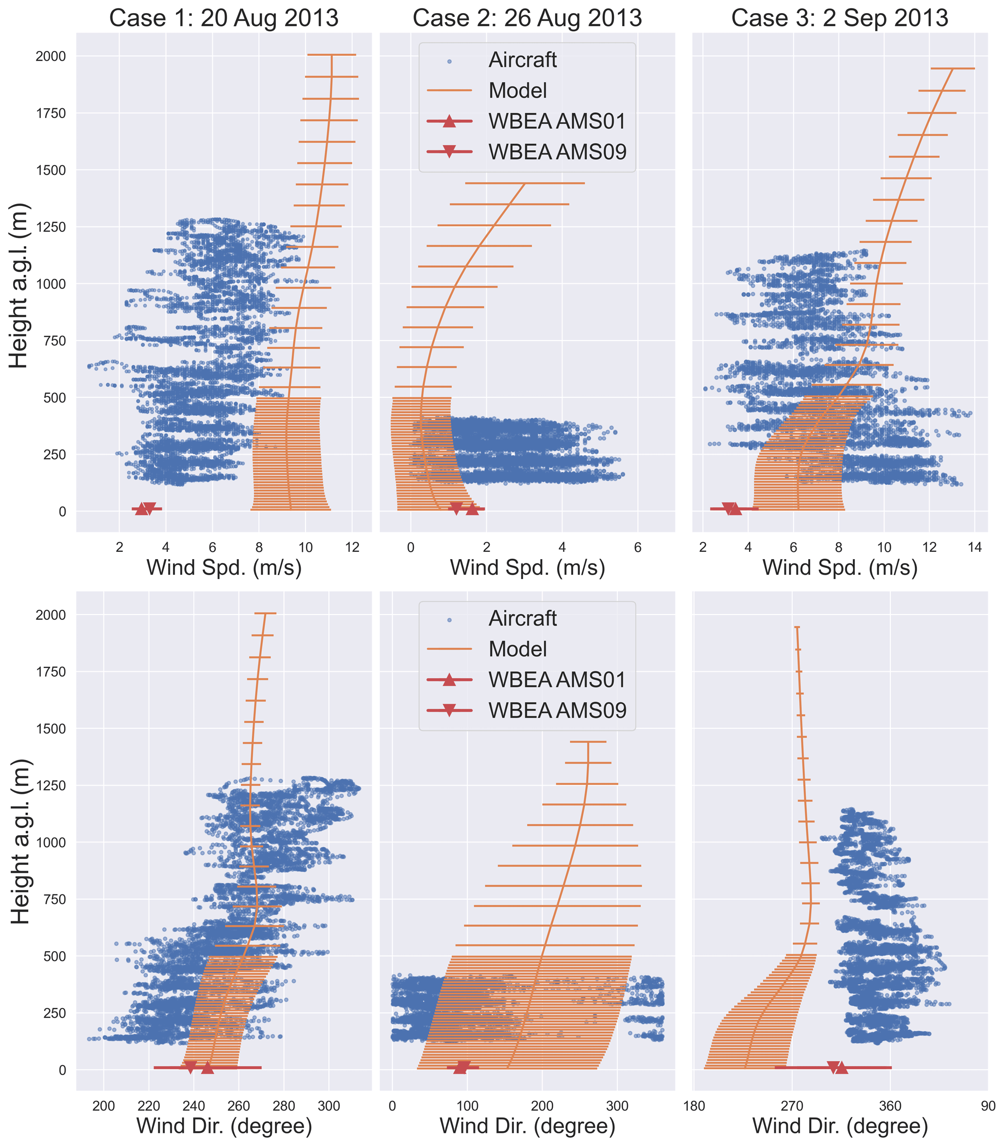
Figure 5Model-generated wind fields (orange) compared to aircraft observations (blue dots) at several altitude levels during the JOSM 2013 airborne campaign and WBEA observational data at 10 m a.g.l. (red triangles). Aircraft data were measured during the 1–2 h box flight portion of the sampling period. Model data are averaged over domain d05 and the simulation time. Horizontal bars show 1 standard deviation in model wind fields (the sum of standard deviations in space and time).
We also compared wind fields from domain d05 to aircraft observations during the JOSM 2013 campaign over the oil sands region for the same time periods as our model simulations (ECCC, 2013). Figure 5 compares model wind speeds and directions for our three cases to aircraft observations for altitude levels of airborne measurements. Model data were averaged horizontally over domain d05 and the simulation time (Fig. 5) for comparison to aircraft data that were collected during a 1–2 h flight time over the oil sands region. Note that the near-surface increase in wind speeds in Fig. 5 is the result of averaging over varying (complex) topography (see Fig. S2 for instantaneous profiles at the location of the main CNRL stack). WBEA data at 10 m a.g.l. are also included in the figure for comparison. Horizontal bars in Fig. 5 show 1 standard deviation in model-generated fields over domain d05. Model wind fields (vertical profiles) overlap with aircraft observations within 1–2 standard deviations. WBEA wind speeds are on average lower than aircraft-measured values for all the cases and are less than model wind speeds for cases 1 and 3. Note the high spatial heterogeneity in wind fields captured by both aircraft observations (Fig. 5, blue dots) and model simulations (Fig. 5, orange bars). Spatial (horizontal and vertical) variability in wind fields was larger for case 2 compared to the other two cases. We discuss in Sect. 3.5 how the conditions of case 2 resulted in weak advection of tracer mass and rendered this case unsuitable for mass-balance retrievals.
3.3 Plume characteristics
In this section we briefly discuss plume behaviour for our three case studies, with an emphasis on case 1 as our main case. Continuous passive-tracer emissions for surface and stack sources were initiated simultaneously at different locations within the finest-resolution modelling domain (d05) after a 30 min initial model spin-up time. Source locations, spatial extent, and release heights are provided in Table 2. Figure 6 shows tracer plumes for case 1 on 20 August 2013 at 17:35 UT, 2 h and 5 min after the initial release. For the example shown, tracer plumes have propagated the downwind span of the modelling domain and reached the opposite lateral boundary. The mean direction of wind for the first 1.5 h of the simulation for this case was from the south-west, which transitioned into winds from the west and west–south-west in the following hours (Fig. 6). As mentioned before, we have discarded 100 grid points from the lateral boundaries of the domain and considered output data for the inner sub-domain in our analysis. The mass-balance calculations discussed in Sect. 3.4 are for the period after 16:30 UT (30 min after 1 h spin-up), as the addition of tracer mass through source emissions and removal via advective and turbulent fluxes through the boundaries of the control volume (box) have reached a mass balance and a relative steady state by this point in the simulation time.
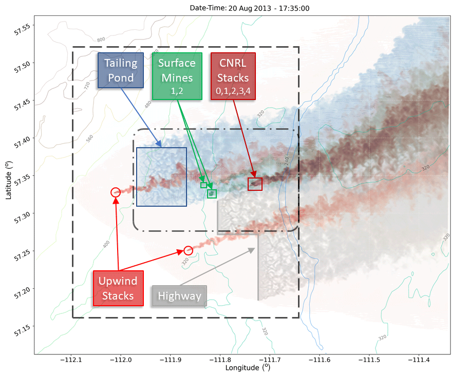
Figure 6The top view of the modelling domain (d05) and the locations of the tracer emission sources are shown. Sources include a large-area source (pond), a multi-segment line source (highway), two small-area sources (mines 1 and 2), five CNRL stacks (0–4), and two upwind point sources (west and south). Emission plumes from the pond are shown in blue, the highway in grey, mines in green, and stack and point sources in red. Colour darkness is proportional to the log of the column total tracer mass. Two control volumes (dark dashed boxes) for 4D mass-balance calculations are shown, one enclosing all the emission sources and the other marking the boundaries of the CNRL facility (the smaller box) and only including within-facility sources.
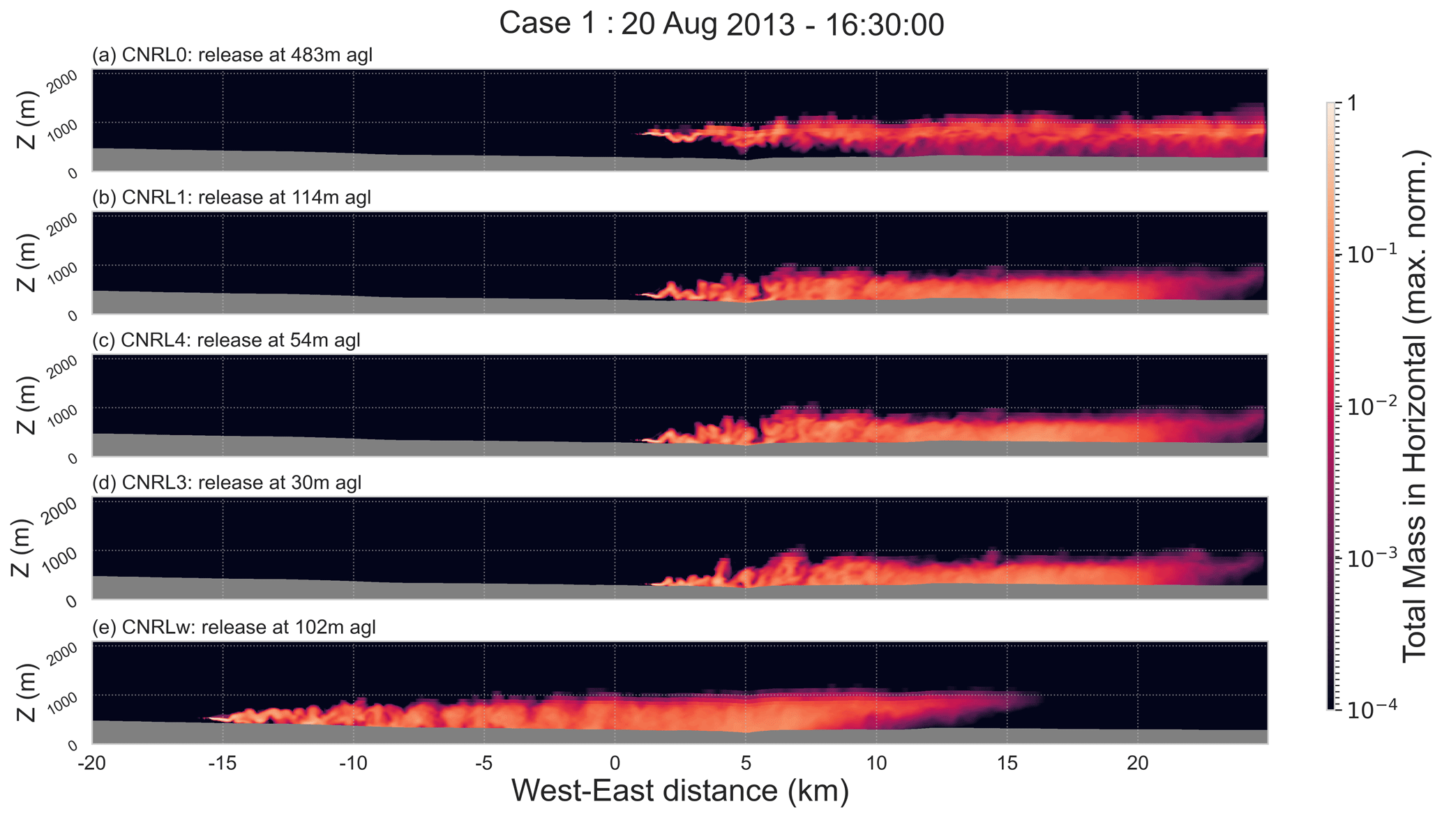
Figure 7Domain d05 west–east vertical cross section for case 1 on 20 August 2013. Vertical cross sections of tracer plumes from stack or point emission sources are shown. The release height above the ground is indicated for each source. Data shown are the tracer amount summed in the horizontal level and normalized to the maximum value for each source. The origin for the west–east distance in kilometres is at the domain centre.
Tracer amounts were advected at different vertical levels and flow regimes. Flow was different at other vertical levels. For instance, surface emissions from MINE1 and MINE2 (Fig. S4, top right panel) were advected in slower air flows and covered a lower downwind range (downwind distance from the point of release) during the same time period compared to stack (elevated) emissions CNRL0–4 (Fig. S4, top left panel). Figure 7 shows a west–east vertical cross section of the modelling domain, with tracer plumes from selected stack or point emission sources. Advection in the west–east orientation is unidirectional at all the vertical layers, as can be seen in Fig. 7. The plume centre line for CNRL0 emissions remains near the initial release height while mixing in the vertical as it is advected downwind. CNRL1–4 emissions, although released at different heights above the ground (by a few tens of metres), show similar vertical mixing profiles along the downwind advection path. Emissions from CNRL1 to CNRL4 mixed with the ground surface within the 5 km range and assumed a near-uniform vertical mixing beyond the 15 km downwind distance. Note how plumes from these sources interact with the Athabasca River basin at the 5 km distance. There is an apparent discontinuity in tracer concentrations beyond which mixing in the vertical is intensified. This is likely due to different surface fluxes over the river and the ground on either side with stronger updrafts. This interaction is less visible in the CNRLw plume, which is relatively well-mixed by the 5 km distance, but it can be seen that the vertical mixing becomes more uniform on the other side of the river for this plume.
Wind and therefore transport in the south–north direction were weaker than the transport in the west–east direction. There was also a strong vertical shear in south–north wind (V). See Appendix Fig. C1 for the meteorological vertical profiles for this case. While all tracer plumes for release heights of 30 m to 114 m a.g.l. were advected north, CNRL0 at 483 m a.g.l. was advected south (Fig. S5, top panel). Similar atmospheric processes governed the dispersion and transport of tracer plumes from the surface emission sources (see Fig. S6).
WRF model simulations for case 2 for the period on 26 August 2013 started at 18:00 UT. As mentioned before, the JOSM box flight (see Sect. 2.1) for this day was rejected for emission rate calculations due to low and variable wind speeds as reported in Fathi et al. (2021). This case is referred to as “rejected” throughout this work. We recreated the meteorological and tracer transport conditions on this day with our super-resolution simulations, which are presented here as an example of unsuitable conditions for top-down retrieval. For this case, tracer emissions from various sources were initiated at 18:30 UT. During the period between 19:00 and 21:00 UT, wind fields over the region of interest were highly variable (spatially) with very low wind speeds (Fig. S7). For case 2, wind speeds at a height of 10 m a.g.l. were less than 5 m s−1 over the modelling domain. The mean wind direction was towards the south and south-west near the ground, transitioning towards the south-east up to 1000 m a.g.l. and towards the east and north-east above 1000 m a.g.l. The south–north wind component V ranged from −1 to 1.5 m s−1 in the vertical, with the west–east wind component U ranging from −0.5 m s−1 near the ground surface to 7.5 m s−1 up to 2500 m a.g.l. See Appendix Fig. C2 for meteorological vertical profiles for this case. The weak advection and the strong vertical wind shear resulted in tracer plumes being transported for only a few kilometres in the horizontal and mainly staying within the boundaries of the CNRL facility (Fig. S7).
Unstable atmospheric conditions persisted during the simulation period over the region of interest for case 2. Gradient Richardson number (Ri) values, which are a measure of atmospheric dynamic stability (Fathi et al., 2021), were below the critical value of Ric=0.25 up to 400 m a.g.l. Ri values below 0.25 correspond to unstable conditions in the atmosphere (AMS, 2022). As a result of (thermal and dynamical) unstable conditions, tracer plumes from emission sources mixed in the vertical up to 2000 m during the simulation time. Similar meteorological and atmospheric conditions were observed during the JOSM 2013 field campaign for the same period. These conditions were also simulated using the Environment and Climate Change Canada (ECCC) air quality model GEM-MACH at 2.5 km resolution. Our super-resolution (50 m) WRF model simulations were also successful in recreating the conditions on 26 August 2013 over CNRL. See Sect. 4.2 in Fathi et al. (2021) for detailed discussions on how low and variable wind and unstable conditions affect the atmospheric transport of tracer plumes for this case.
Case 3 model simulations at super-resolutions for the period on 2 September 2013 started at 15:00 UT. Tracer emissions were initiated at 15:30 UT. Atmospheric conditions during this case were fairly constant, with the Gradient Richardson number Ri below the critical value Ric=0.25 (indicating unstable conditions) up to 100 m a.g.l. Note that, for this case, similar to the other two cases, atmospheric conditions were unstable (both thermally and dynamically) within the bottom one-third to one-half of the atmospheric boundary layer (ABL). Wind speeds were higher for this case compared to the other cases, with the west–east wind component U ranging from 5 m s−1 near the ground surface to 15 m s−1 up to 2000 m a.g.l. The south–north component of the wind V was about 5 m s−1 near the surface, with a strong shear in the vertical transitioning towards the south at about 500 m a.g.l. See Fig. C3 for meteorological vertical profiles during the time period of this case. Similar to case 1, the mean direction of transport was towards east and north-east but with a stronger northward component compared to case 1 (see Fig. S8).
Average inversion heights Zi (inferred from potential temperature θ profiles) for the three cases are marked with dashed lines in Figs. C1, C2, and C3. Zi for cases 1 and 3 was between 300 and 400 m a.g.l., placing the tracer sources (all except CNRL0) within the ABL, where turbulent mixing plays a dominant role in modifying the vertical structure of the atmosphere, including tracer concentrations. As a result, tracer amounts released from these sources (at different heights) were mixed quickly in the vertical extent of the ABL within the 10 km downwind distance, resulting in similar uniform vertical profiles (Fig. 7). For cases 1 and 3 the CNRL0 release height at 483 m a.g.l. was above Zi, where turbulent mixing is suppressed by the negatively buoyant atmosphere in the stably stratified inversion layer, which confined the dispersion of CNRL0 tracer amounts to a smaller vertical extent detached from the ground surface up to 10 km downwind distance (see Fig. 7). For case 2, Zi was between 1400 and 1500 m a.g.l., placing all the sources, including CNRL0, well within the ABL and resulting in similar vertical mixing for tracers released at different heights from the ground surface up to 483 m a.g.l. and in the downwind distance (see Fig. S9).
3.4 Model global tracer mass conservation and emission rate calculation
In this section we evaluate the conservation of tracer mass within domain d05. As discussed in Sect. 2.2, in our simulations we used a positive-definite transport scheme combined with a sixth-order diffusion scheme. Negative up-gradient diffusion flux near sharp concentration gradients resulted in partial creation of erroneous mass within the modelling domain. Positive flux and monotonicity can be enforced in the model by setting negative fluxes to zero; however, this is not mass-conserved (see Fig. S10). Therefore, we configured our simulation using the diffusion scheme without the monotonic option. We investigated the tracer mass budget within domain d05 by integrating over the entire domain at each model output time step (Eq. 2). Figure 8 shows the ratios of mass present in the modelling domain at each time stamp to the total mass emitted up to that point. The ratios are for the 11 emission scenarios for the first hour after tracer release was initiated. The net mass present within the modelling domain is separated into negative and positive masses. Time series are shown as the ratio of mass present in the domain to the mass emitted (normalized) for each emission source. Initially, up to 14 % negative mass (Fig. 8c) is created within the domain, which is offset by about the same amount of excess positive mass creation (Fig. 8b). The net mass (Fig. 8a) is conserved as the negative and excess positive masses cancel out. The creation of negative mass is reduced over the simulation time until it falls below 2 % after about 30 min of simulation time. The creation of negative mass is likely due to sharp gradients in tracer mass immediately after the initial release that are concentrated mostly upwind of the emission sources. As tracer mass is advected and dispersed over several grid points, the gradient is smoothed out and negative mass creation becomes less pronounced. The present-to-emitted mass ratios for 10 out of 11 sources are conserved and remain equal to unity up to about 16:30 UT, when they reach the domain boundaries and are removed from the modelling domain (Fig. 8a). The exception is CNRL0, which does not keep up with the emissions and, except for a few minutes after the initial release, is always less than one. The mass present in the domain (not normalized) increases initially and later plateaus (approaching an asymptote) as plumes start exiting through domain boundaries at rates less than or equal to source emission rates. Similarly, the decrease in the present-to-emitted mass ratio in Fig. 8 (marked by a vertical line) is a result of tracer mass exiting through domain boundaries at rates less than or equal to source emission rates (and is not a violation of model mass conservation).
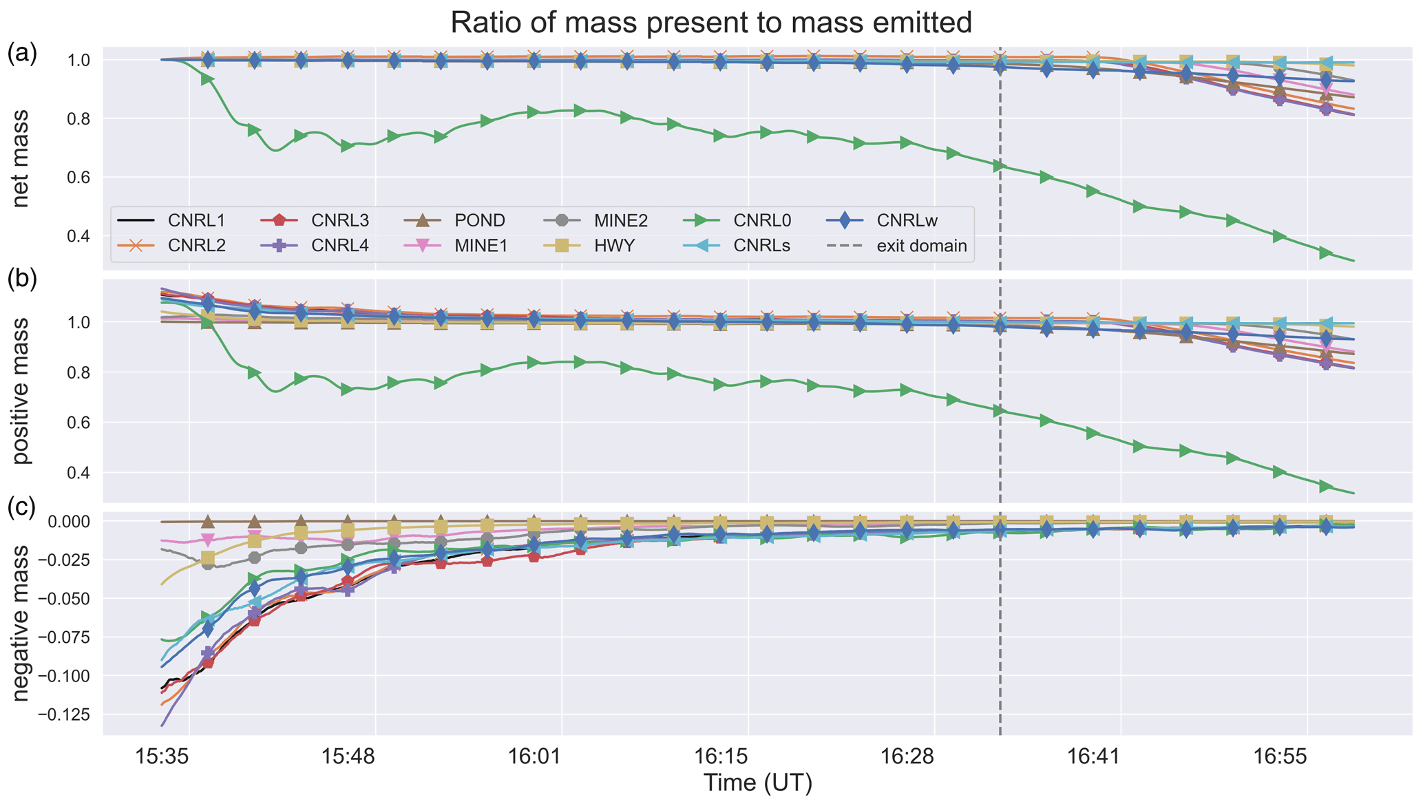
Figure 8The ratio of the tracer mass present within the modelling domain to the mass emitted over the simulation time after the start of tracer release. Time series are separated into positive and negative masses in panels (b) and (c). Tracer mass remains conserved over time, with the exception of CNRL0. Note that the drop in the present-to-emitted mass ratio beyond 16:30 UT, marked by the vertical dashed line, is due to the tracer mass exiting through domain boundaries and is not a violation of mass conservation.
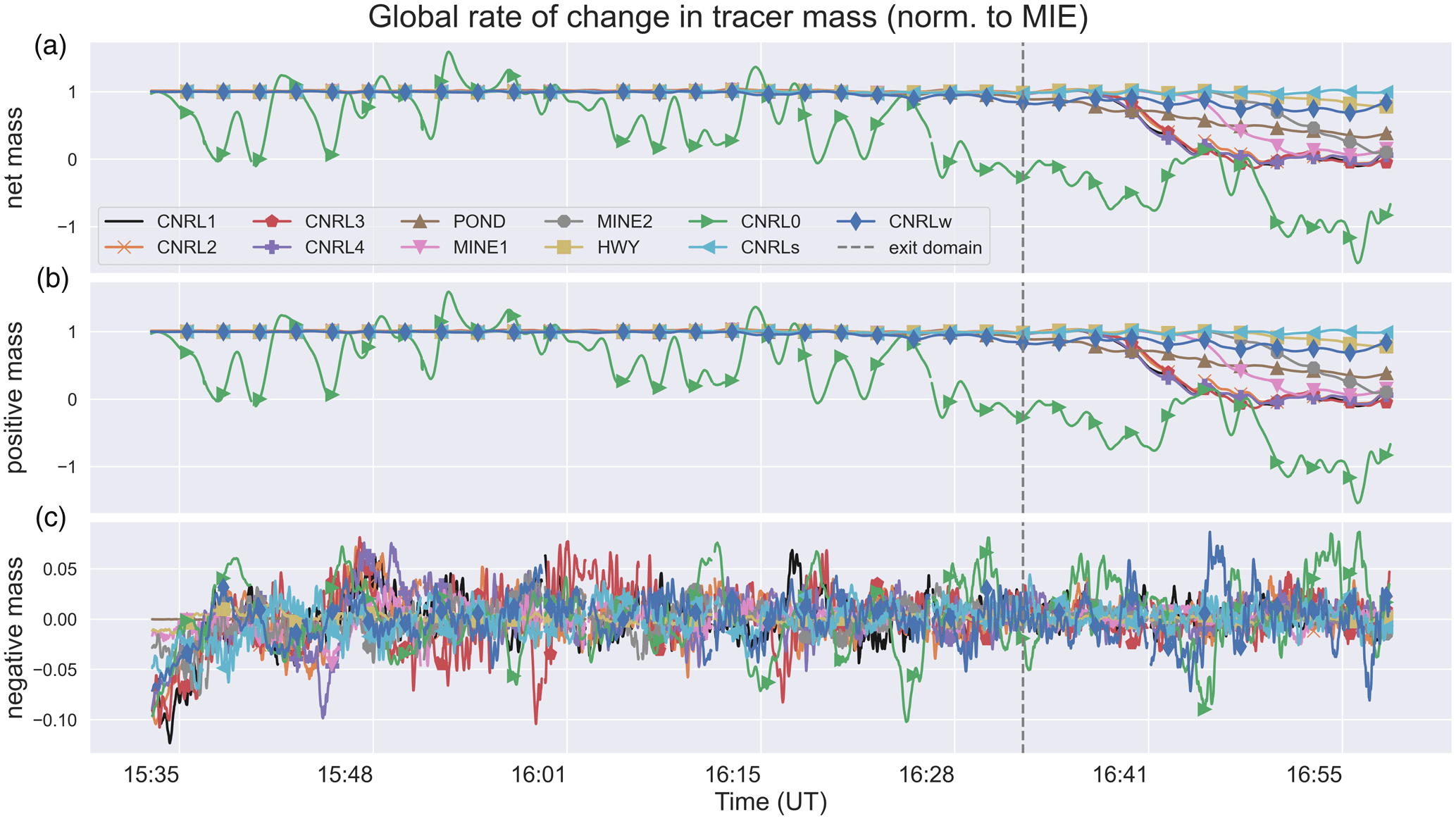
Figure 9The temporal rate of change in tracer mass for the entire domain SC,d05 is shown. Time series are normalized to model input emission (MIE) rates. The net rate of change (a) is separated into rates for positive and negative masses in panels (b) and (c). The creation of negative mass is offset by the creation of excess positive mass. The rate of change in the tracer mass matches MIE (conserved) for all except one emission source (CNRL0).
Figure 9 shows the temporal rate of change in tracer mass for each emission scenario, normalized to the model input emission (MIE) rate. This rate of change was calculated by differentiating the domain mass time series shown in Fig. 8 according to Eq. (3), which is equivalent to the storage rate term for the entire domain (SC,d05). The net rate of change (panel a) is separated into rates for positive and negative masses in panels b and c for each tracer case. The rate of creation of negative mass oscillates between −10 % and 5 % and is damped over time. This is offset by the creation of excess positive mass, resulting in net mass conservation over the modelling domain (an artifact of the model transport scheme). For tracer mass to be conserved, the net rate of change over the entire domain must be equal to the model input emission rate for the time period before tracer plumes start exiting through domain boundaries (before about 16:30 UT for most tracers, as shown in Fig. 9). Tracer mass at domain boundaries was set to zero (boundary condition). As plumes reached the boundaries, the tracer mass was removed from the domain (at different times for each tracer depending on the transport speed and source proximity to the boundaries), hence the drop in SC,d05 as shown in Fig. 9. This was true for all emission scenarios, as can be seen from Fig. 9a. The SC,d05 time series for 10 out of 11 sources were at the MIE level, indicating mass conservation for these cases. The only exception was CNRL0, for which SC,d05 oscillated around the MIE without converging. It is evident from Figs. 8 and 9 that CNRL0 mass was not conserved.
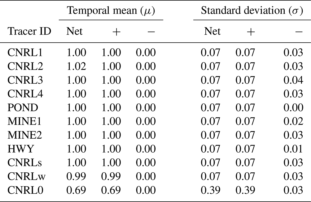
For the case of CNRL0, tracer release height was at the model vertical level where model resolution (vertical) transitions from a model layer thickness of about 12 m to progressively increasing thicknesses (and decreasing resolutions). Transport (advection and diffusion) of tracer amounts between model vertical layers of varying resolutions likely intensified erroneous and unbalanced (by excess positive mass) creation of negative mass (in both magnitude and spatial location). While the positive-definite transport scheme ensures positive and conserved advection of tracers, the negative up-gradient diffusion can still create erroneous mass. Our results suggest that this is intensified on a non-uniform grid (varying grid sizes). However, more in-depth investigation (beyond the scope of this paper) is required to confirm such effects. Table 6 lists statistics for the first hour of tracer emissions (before exiting through domain boundaries) for all emission scenarios. The temporal means (μ) and standard deviations (σ) are indicated for the normalized rates (SC,d05) shown in Fig. 9. As mentioned before, CNRL0 is the only non-conservative case with a mean value of 0.69 and a standard deviation of 0.39. Therefore, in this paper and in Fathi (2022), we discuss CNRL0 mainly in terms of plume behaviour rather than a conserved quantity in mass-balance calculations. The mean normalized rates for CNRL2 and CNRLw were within 2 % and 1 %, respectively, of MIEs. For the remaining 8 out of 11 cases, the mean normalized rates were equal to 1.00 (strong agreement with model input emission rates). These results apply to all three case studies within 2 %–4 %.
Table 6Normalized (to MIE) rates of change in tracer mass for all emission scenarios are shown. Mean rates are given for net, positive (+), and negative (−) masses. Standard deviations are also provided. Rates agree with model input emissions within 2 % for 10 out of the 11 tracers (conserved).
3.5 Local mass-conservation and mass-balance analysis
Results in Table 6 indicate global (over the entire modelling domain) mass conservation for 10 out of 11 emission cases. We further evaluated model local mass conservation through mass-balance and flux calculations in order to assess the model's ability to be used for accurate mass-balance assessment. A control volume enclosing all the emission sources, with the downwind wall at a distance of 5 km from the main CNRL stacks, was considered (large rectangle in Fig. 6). We conducted 4D mass-balance calculations using this control volume for all the case studies to evaluate the performance of model simulations in the context of local mass conservation and transport of tracer amounts within a sub-domain (control volume). The mass-balance calculations for this portion of our analysis were conducted for the period between 1 and 2 h after the tracer release started, well after plumes crossed the box (control volume) walls.
Mass-balance calculations were done according to Eq. (6). The net flux-out term FC,out was calculated using the instantaneous fields (e.g. wind speed, tracer concentrations) along the top and lateral boundaries of the control volume. FC,out includes horizontal (FC,H, FC,HT) and vertical (FC,V, FC,VT) advective and turbulent fluxes across box walls. The rate of mass storage or release SC within the control volume (box) at each model output time step (1 s) was calculated by integrating over the entire volume of the box and differentiating with respect to time. Source emission rates EC were calculated as the sum of FC,out and SC and were compared to MIE rates. Contributions (absolute value) of different terms are shown in Fig. 10 for case 1. The main contribution came from the horizontal advective flux, along with significant contributions from the storage rate term SC. The horizontal turbulent flux contributed between −0.3 % and 2.3 % for the three cases. Contributions from vertical fluxes were negligible as the box top was chosen at a height of over 4 km a.g.l., well above the mixing layer height at about 2–3 km a.g.l. The breakdowns of contributing terms for the three cases are summarized in Table 7.
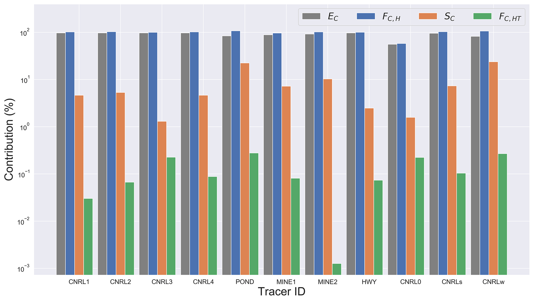
Figure 10Normalized (to MIE) retrieved emission rates for tracer emission scenarios of case 1. Emission rates (EC) were calculated using the mass-balance equation Eq. (6) and the control volume shown in Fig. 6. The breakdowns (%) of the contributing terms are shown as absolute values; see Table 7 for the actual values. The vertical axis is in the log scale. Refer to Table 2 for the source specifications.
For case 1, mass-balance estimates were within 4 % of the MIE rates for 10 out of 11 tracers (see Table 7). Estimates for the (globally) non-conservative tracer CNRL0 were biased low by 51 %. Estimated emission rates for all the other emission scenarios were in over 96 % agreement with the MIEs. Contributions from the storage rate term SC were negative (release of mass from the control volume) and ranged between 1 % and 30 %. FC,H contributions were positive, ranged between 51 % and 130 %, and were offset by negative SC contributions. Our results with GEM-MACH model simulations in Fathi et al. (2021) for SO2 emissions (stack or point source) for the same time period were very similar (97 % FC,H and 3 % SC) to stack emissions simulated here with WRF at super-resolution. The model-based study by Panitz et al. (2002) attributes 85 % to 95 % of the emissions to advective fluxes (for SO2 and CO), which is also consistent with our estimates. Our results here with WRF (LES) simulations are within the ranges of previous model studies.
Table 7Source emission rates (EC) determined by performing mass-balance calculations on model output data, evaluated against MIE for the three cases. Results are shown as normalized mean bias (nmb) in percentage. Contributions of the three main terms in the mass-balance equation are shown, normalized to MIE (%). Values less than 0.1 % are indicated with ε.
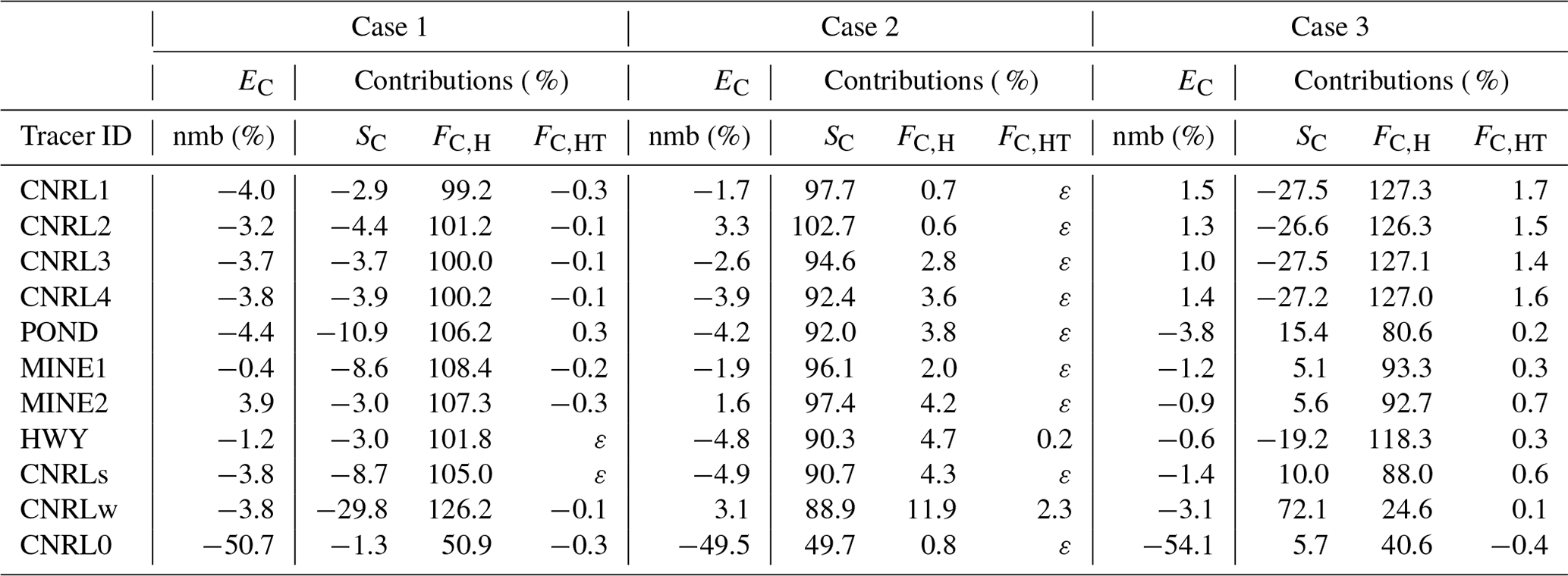
Mass-balance estimates for case 2 were within 5 % of the MIEs for the 10 emission scenarios (Table 7). Estimates for CNRL0 were biased low, similar to case 1, by about 50 % (not conserved). For this case, where wind speeds were very low and spatially heterogeneous, the tracer amounts were mainly stalled within the control volume over the simulation time. Consequently, the storage rate term SC was the dominant term, with contributions (positive) ranging from 89 % to 103 %. The horizontal advective flux FC,H contributed to the mass-balance equation between 0.6 % and 12 %. The contributions from vertical and turbulent fluxes were less than 1 %, except for CNRLw with a 2.3 % contribution. Our estimates for SO2 emission rates for CNRL with GEM-MACH simulations in Fathi et al. (2021) showed similar large storage levels. We note that conditions of weak advection were also observed during the JOSM 2013 airborne campaign for the period of case 2 on 26 August 2013 (see Fig. 5), which resulted in negligible estimated emission rates based on flux calculations alone (i.e. not accounting for storage). As a result of such conditions, the emission estimation flights for this time period were not included (rejected) for top-down retrievals in the post-campaign studies. Note that GEM-MACH model simulations at 2.5 km resolution for the same case (26 August 2013) predicted a storage contribution of only 43 % (Fathi et al., 2021), whereas WRF super-resolution simulations in this work predicted a contribution of ≥89 %. While both modelling set-ups replicated the same meteorological (advection) conditions, the relatively coarser resolution of GEM-MACH simulations resulted in larger computational (grid) diffusion and consequently larger downwind dispersion of tracer amounts (and larger predicted horizontal mass flux). This in part demonstrates the benefits of employing super-resolution over high-resolution modelling. The WRF super-resolution simulations in this work were successful in closely replicating the observed weak advection conditions and GEM-MACH-predicted % for the same period (Fathi et al., 2021) but at a higher spatio-temporal resolution.
Mass-balance estimates for case 3 were similar to estimates for case 1, with over 96 % agreement with MIEs for the 10 emission scenarios. Similar to case 1 and case 2, CNRL0 estimates were biased low (at 54 %). For case 3, the contribution of the storage rate term SC ranged between −27.5 % and 72.1 %. The horizontal advective flux FC,H contributed between 25 % and 127 % to the mass-balance equation. The horizontal turbulent flux contributed between −0.4 % and 1.7 %. Similar to case 1 and case 2, contributions of vertical fluxes were negligible.
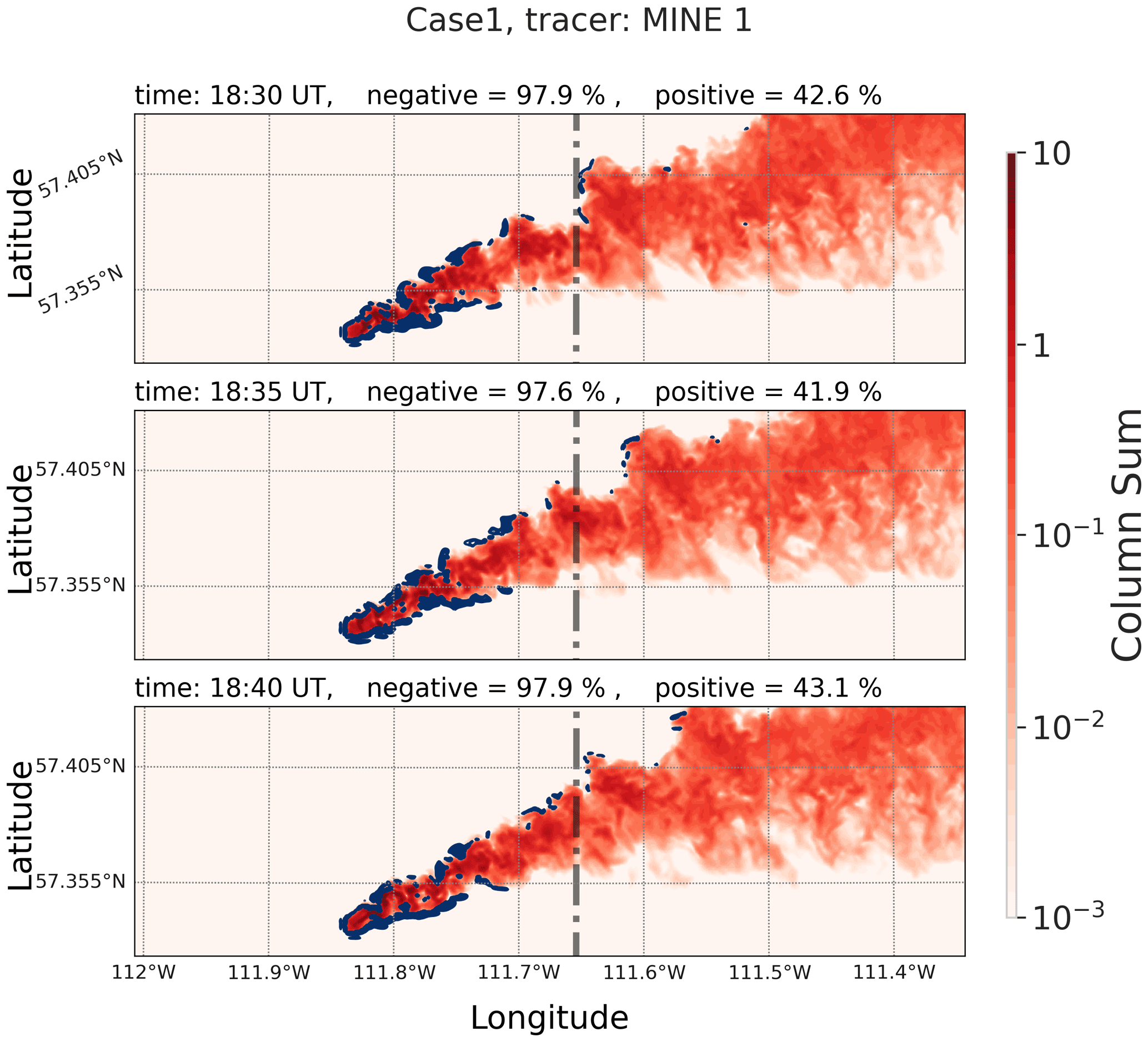
Figure 11Three-panel snapshot of the MINE1 plume during case 1 at 5 min intervals. Note that the erroneous negative mass creation (blue contours) is concentrated upwind of the emission source and on plume edges. Consequently, 98 % of the domain's total negative mass was located within the control volume, along with only 43 % of the total positive mass (red). The vertical dashed line shows the location of the control volume downwind wall.
As can be seen from Table 7, our mass-balance estimates for the three cases were within 5 % of the MIEs. Estimates were partially affected by local mass deficit or surplus for these cases. As discussed at the beginning of this section, the turbulent diffusion step in our WRF model set-up created erroneous negative mass (locally) within the modelling domain. The negative mass was mainly created near the emission source (upwind) and at plume edges, as indicated in Fig. 11. The advection of positive or negative masses that passed the box downwind wall (vertical dashed line in Fig. 11) was not always balanced due to different spatial distributions for positive and negative amounts. Figure 11 shows three snapshots at 5 min intervals for tracer MINE1 during the final hour of case 1. As indicated in the figure, during this time period, 98 % of the domain total negative mass remained inside the control volume along with only about 43 % of the domain total positive mass. This resulted in a mismatch between the negative mass, the excess positive mass, and the consequent mass emission rate underestimations for this and similar cases. Estimates were also partially affected by the changing vertical grid spacing for the upper model layers for tracer amounts mixing to higher altitudes (>500 m). This is similar to mass loss for CNRL0 emissions but to a much lesser extent. We conclude that all three cases (with 10 emission scenarios) were globally (in the entire modelling domain) and locally (control volume) mass-conserved within 4 % and 5 % of the MIEs, respectively.
We developed and implemented super-resolution (<100 m) model simulations employing the WRF-ARW atmospheric modelling system. We used NARR data at 31 km resolution as initial and boundary conditions for our coarsest domain at the same resolution. Dynamical downscaling of reanalysis data was done through numerical model nesting with five domains from 31 km to 50 m at the finest-resolution domain over the CNRL oil sands facility. We chose our model simulation times and locations from three emission rate retrieval flights during the JOSM field campaign in August and September 2013. We performed model simulations for 3 d in August and September representing different meteorological conditions. Model simulations for the finest-resolution domain were conducted using large-eddy-simulation (LES) sub-grid parameterization. The main objective was to model the state of the atmosphere at a high enough resolution to simulate atmospheric dynamical processes at spatial and temporal scales of airborne measurements while ensuring local and global mass conservation. Model output data from our simulation cases were evaluated against historical observational data from two WBEA monitoring stations and aircraft observations during the JOSM 2013 campaign for the same locations and time periods. Model output fields showed good agreement with observational data within 5 ∘C for 2 m temperature and 1 %–25 % for 2 m relative humidity. General wind directions generated by the super-resolution model were within 20 to 30∘ of the observational data. Model wind speeds were in agreement with aircraft observations within 1–2 standard deviations.
We modified the WRF model dynamical-solver source code to simulate passive-tracer emissions within the finest modelling domain centred over the CNRL facility. Our case simulations included 11 different emission scenarios with stack–point and surface–area sources. Continuous emissions were simulated for time periods of 2–3 h during 3 different days. We evaluated the atmospheric dispersion and transport of tracer plumes from the 11 emission scenarios under different meteorological conditions. Unstable atmospheric conditions, low wind speeds, and strong vertical wind shear during our case study on 26 August 2013 resulted in weak advection of tracer plumes during the simulation time. During the case studies on 20 August and 2 September, atmospheric conditions were less variable and the vertical wind shear was weak, with higher wind speeds of about 5–15 m s−1. Tracer plumes from emission sources were advected mainly towards the east and north-east for these two cases. Similar conditions were observed during the JOSM 2013 field campaign for the same time periods and locations as our three case studies.
We evaluated the performance of our model simulations in terms of global (over the entire domain) mass conservation. For 1 case out of 11, creation of erroneous mass by the model transport step resulted in loss of tracer mass. For this emission case, tracer release was placed at the model vertical level where model vertical resolution transitions from the super-resolution of about 10 m to progressively coarser resolutions. Our results suggest that the unbalanced creation of erroneous mass at sharp concentration gradients, such as in the vicinity of point sources, is intensified on an irregular grid (an artifact of model dispersion). However, more investigation with longer simulation times (beyond the scope of this paper) is required to investigate such effects further. Small negative diffusive fluxes and the use of the positive-definite re-normalization scheme in our modelling set-up prevented non-physical effects (e.g. negative mass creation) for 10 out of 11 emission sources (assigned on a regular grid). The rate of change for tracer mass was calculated by integrating over the entire modelling domain and differentiating with respect to time. Results were within 2 %–4 % of model input emissions (MIE) for 10 out of 11 emission scenarios, indicating global mass conservation in our simulation cases. Therefore, it is recommended that tracer emissions be assigned to model grid points with regular grid spacing for several adjacent model cells along the x, y, and z directions.
We further investigated local mass conservation by mass-balance calculations over a sub-domain (control volume). Mass-balance calculations were conducted by considering a control volume (box) enclosing all the emission sources. We estimated within-box source emission rates by calculating the net exiting flux through box top and lateral walls as well as the temporal rate of change in tracer mass within the control volume. Under normal advective conditions (>5 m s−1 wind speeds), the horizontal advective flux was equal to over 90 % of the emission rate, while turbulent fluxes were less than 2 %. The remaining contribution came from the storage rate term, the release, and the accumulation rate of tracer mass within the control volume. Our mass-balance estimates were within 5 % of MIE for tracer sources, with release heights within the bottom 40 model vertical layers (with regular vertical grid spacing) for our three case studies (30 emission scenarios), indicating local mass conservation for our super-resolution WRF simulations. Again, this suggests that assigning tracer release on a regular grid (horizontal and vertical) would ensure mass conservation using the available WRF model mass-conservation schemes.
Except for one hypothetical emission source, our results for various tracer emission scenarios under different meteorological conditions were globally and locally mass-conserved within 4 % and 5 %, respectively, of model input emission rates. In Fathi (2022), we use the model output from super-resolution WRF simulations discussed here for a model-based study of airborne top-down source emission rate retrievals, where we evaluate the conventional methods and propose improved approaches for aircraft-based retrievals.
The WRF model eddy viscosity (diffusivity) for the predicted turbulent kinetic energy option (K option km_opt=2) is computed using (Skamarock et al., 2008)
where e is the turbulent kinetic energy (prognostic in this scheme), Ck is a constant (typically ), and l is a length scale given as follows for the anisotropic option:
where N is the Brunt–Väisälä frequency: see Skamarock et al. (2008) for derivations. The eddy viscosity used for mixing scalars is divided by a turbulent Prandtl number Pr. The Prandtl number is for the horizontal eddy viscosity Kh and for the vertical eddy viscosity Kv. Note that the above parameters and values are for the anisotropic mixing option (mix_isotropic =0, default) that was used in our WRF simulations.
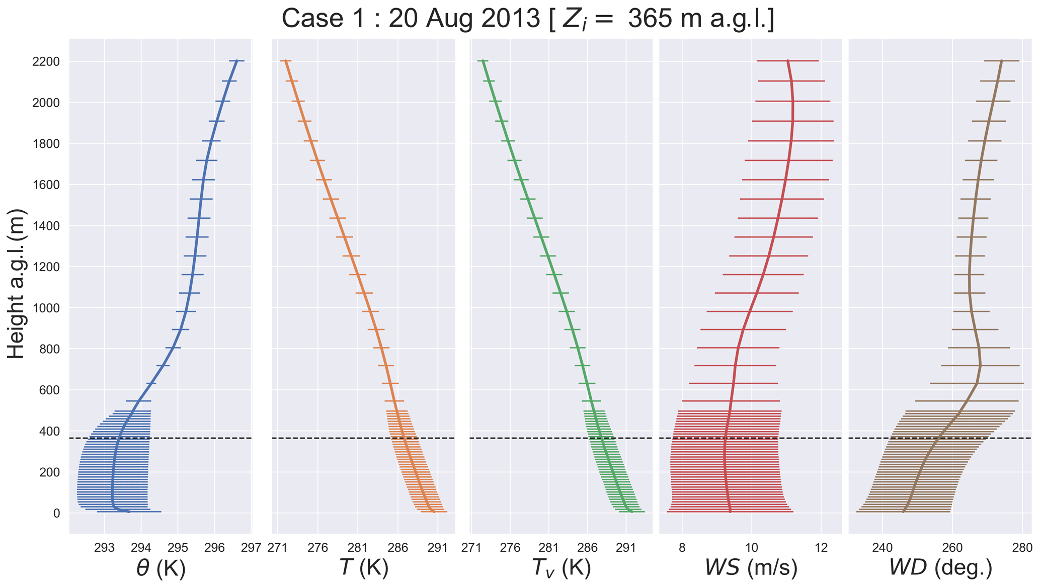
Figure C1Case 1 meteorological profiles on 20 August 2013: potential temperature θ, absolute temperature T, virtual temperature Tv, wind speed WS, and wind direction WD. The profiles were averaged horizontally over domain d05 and over the simulation time. Bars show standard deviations. Inversion height Zi is marked with dashed line.
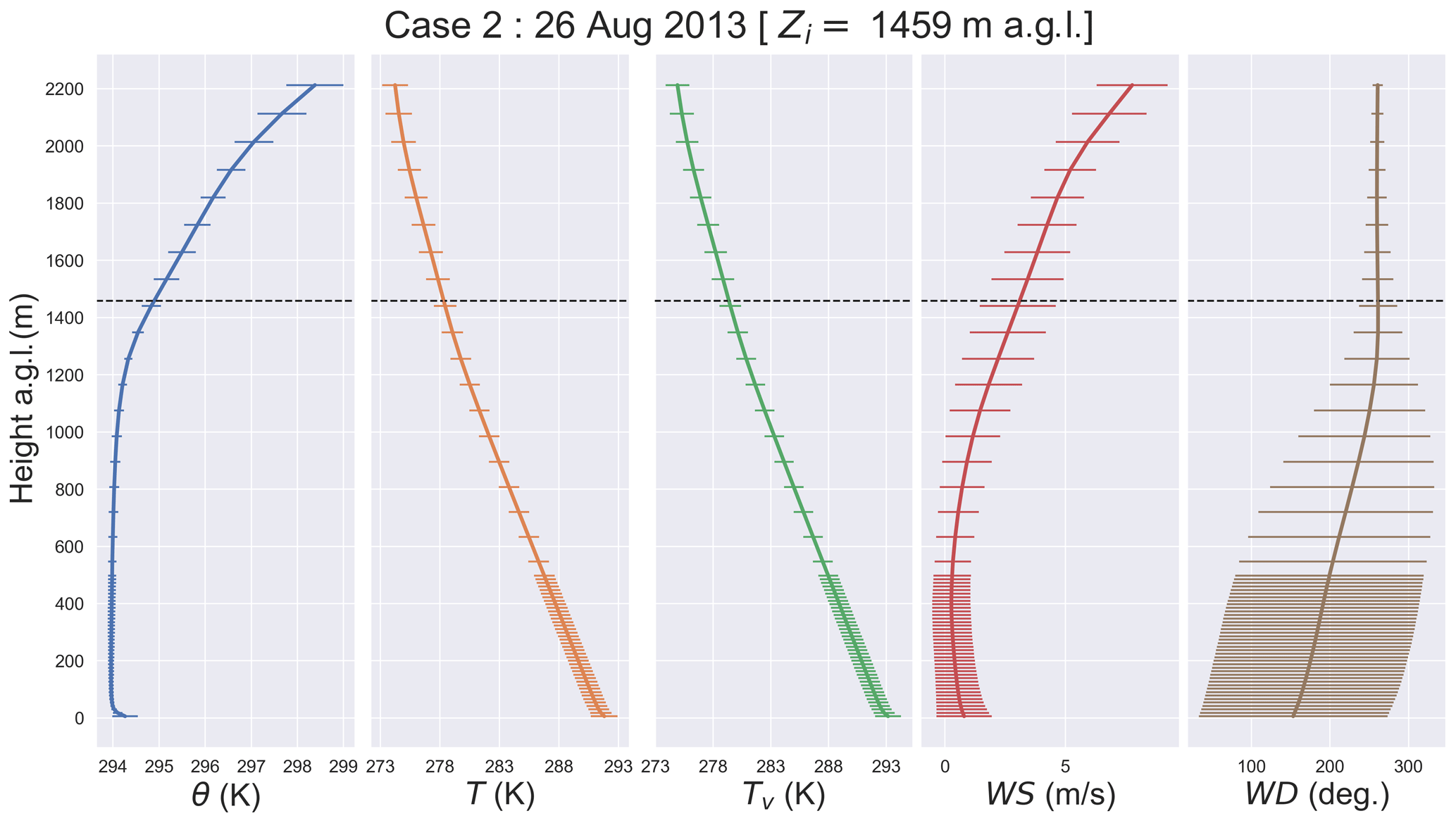
Figure C2Case 2 meteorological profiles on 26 August 2013: potential temperature θ, absolute temperature T, virtual temperature Tv, wind speed WS, and wind direction WD. The profiles were averaged horizontally over domain d05 and over the simulation time. Bars show standard deviations. Inversion height Zi is marked with dashed line.
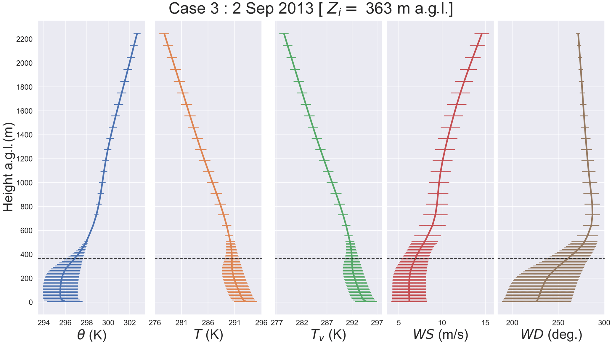
Figure C3Case 3 meteorological profiles on 2 September 2013: potential temperature θ, absolute temperature T, virtual temperature Tv, wind speed WS, and wind direction WD. The profiles were averaged horizontally over domain d05 and over the simulation time. Bars show standard deviations. Inversion height Zi is marked with dashed line.
The release version of WRF-ARW 3.9 used for this study can be downloaded from https://www2.mmm.ucar.edu/wrf/users/download/get_source.html (Skamarock et al., 2008). The North American Regional Reanalysis (NARR) data from the National Oceanic and Atmospheric Administration (NOAA) used as initial and boundary conditions for model simulations in this study can be accessed at https://doi.org/10.5281/zenodo.7302357 (NOAA-Fathi, 2022). The historical observational monitoring data from the Wood Buffalo Environmental Association (WBEA) used for comparison to model output in this work can be accessed at https://doi.org/10.5281/zenodo.7306284 (WBEA-Fathi, 2022). The aircraft measurement data from the JOSM 2013 campaign used in this work are available from the Environment and Climate Change Canada Data Catalogue (https://data-donnees.ec.gc.ca/data/air/monitor/ambient-air-quality-oil-sands-region/pollutant-transformation-aircraft-based-multi-parameters-oil-sands-region/?lang=en, last access: 4 July 2023, ECCC, 2013).
The supplement related to this article is available online at: https://doi.org/10.5194/gmd-16-5069-2023-supplement.
SF set up and ran the WRF-ARW simulations, performed all the analyses using the model output data, and wrote the paper. MG and YC provided advice during planning and analysis and contributed to paper revisions.
The contact author has declared that none of the authors has any competing interests.
Publisher's note: Copernicus Publications remains neutral with regard to jurisdictional claims in published maps and institutional affiliations.
This research was enabled in part by support provided by Compute Ontario (Graham, computecanada.ca), WestGrid (Cedar, computecanada.ca), and the Digital Research Alliance of Canada (https://alliancecan.ca, last access: 4 July 2023). We acknowledge the use of flight parameter information from the ECCC Data Catalogue: Pollutant Transformation, Summer 2013 Aircraft Intensive Multi Parameters, Oil Sands Region.
This research has been supported by the Natural Sciences and Engineering Research Council of Canada (grant no. Discovery Grant RGPIN-2015-04292).
This paper was edited by Jinkyu Hong and reviewed by two anonymous referees.
Ahmadov, R., McKeen, S., Trainer, M., Banta, R., Brewer, A., Brown, S., Edwards, P. M., de Gouw, J. A., Frost, G. J., Gilman, J., Helmig, D., Johnson, B., Karion, A., Koss, A., Langford, A., Lerner, B., Olson, J., Oltmans, S., Peischl, J., Pétron, G., Pichugina, Y., Roberts, J. M., Ryerson, T., Schnell, R., Senff, C., Sweeney, C., Thompson, C., Veres, P. R., Warneke, C., Wild, R., Williams, E. J., Yuan, B., and Zamora, R.: Understanding high wintertime ozone pollution events in an oil- and natural gas-producing region of the western US, Atmos. Chem. Phys., 15, 411–429, https://doi.org/10.5194/acp-15-411-2015, 2015. a
Alfieri, S., Amato, U., Carfora, M., Esposito, M., and Magliulo, V.: Quantifying trace gas emissions from composite landscapes: A mass-budget approach with aircraft measurements, Atmos. Environ., 44, 1866–1876, https://doi.org/10.1016/j.atmosenv.2010.02.026, 2010. a
American Meteorological Society,: Gradient Richardson number, Glossary of Meteorology, http://glossary.ametsoc.org/wiki/Gradient_richardson_number (last access: 4 July 2023), 2022. a
Angevine, W. M., Peischl, J., Crawford, A., Loughner, C. P., Pollack, I. B., and Thompson, C. R.: Errors in top-down estimates of emissions using a known source, Atmos. Chem. Phys., 20, 11855–11868, https://doi.org/10.5194/acp-20-11855-2020, 2020. a
Barkley, Z. R., Lauvaux, T., Davis, K. J., Deng, A., Miles, N. L., Richardson, S. J., Cao, Y., Sweeney, C., Karion, A., Smith, M., Kort, E. A., Schwietzke, S., Murphy, T., Cervone, G., Martins, D., and Maasakkers, J. D.: Quantifying methane emissions from natural gas production in north-eastern Pennsylvania, Atmos. Chem. Phys., 17, 13941–13966, https://doi.org/10.5194/acp-17-13941-2017, 2017. a
Blaylock, B. K.: Tracer Plumes in WRF, https://home.chpc.utah.edu/~u0553130/Brian_Blaylock/tracer.html (last access: 8 March 2023), 2017. a
Blaylock, B. K., Horel, J. D., and Crosman, E. T.: Impact of Lake Breezes on Summer Ozone Concentrations in the Salt Lake Valley, J. Appl. Meteorol. Clim., 56, 353–370, https://doi.org/10.1175/JAMC-D-16-0216.1, 2017. a
Conley, S., Faloona, I., Mehrotra, S., Suard, M., Lenschow, D. H., Sweeney, C., Herndon, S., Schwietzke, S., Pétron, G., Pifer, J., Kort, E. A., and Schnell, R.: Application of Gauss's theorem to quantify localized surface emissions from airborne measurements of wind and trace gases, Atmos. Meas. Tech., 10, 3345–3358, https://doi.org/10.5194/amt-10-3345-2017, 2017. a, b
Cui, Y. Y., Brioude, J., McKeen, S. A., Angevine, W. M., Kim, S.-W., Frost, G. J., Ahmadov, R., Peischl, J., Bousserez, N., Liu, Z., Ryerson, T. B., Wofsy, S. C., Santoni, G. W., Kort, E. A., Fischer, M. L., and Trainer, M.: Top-down estimate of methane emissions in California using a mesoscale inverse modeling technique: The South Coast Air Basin, J. Geophys. Res.-Atmos., 120, 6698–6711, https://doi.org/10.1002/2014JD023002, 2015. a
Daniels, M. H., Lundquist, K. A., Mirocha, J. D., Wiersema, D. J., and Chow, F. K.: A New Vertical Grid Nesting Capability in the Weather Research and Forecasting (WRF) Model, Mon. Weather Rev., 144, 3725–3747, https://doi.org/10.1175/MWR-D-16-0049.1, 2016. a, b
ECCC: Pollutant Transformation, Summer 2013 Aircraft Intensive Multi Parameters, Oil Sands Region, https://data-donnees.ec.gc.ca/data/air/monitor/ambient-air-quality-oil-sands-region/pollutant-transformation-aircraft-based-multi-parameters-oil-sands-region/?lang=en (last access: 4 July 2023), 2013. a, b
Fathi, S.: Evaluating the Top-down Emission Rate Retrieval Algorithm (TERRA) Using Virtual Aircraft-based Sampling Within the GEM-MACH Model, Master's thesis, York University, http://hdl.handle.net/10315/34547 (last access: 4 July 2023), 2017. a
Fathi, S.: Optimizing Top-down Airborne Emission Retrievals through High and Super-Resolution Numerical Modelling, Dissertation, http://hdl.handle.net/10315/40663 (last access: 4 July 2023), 2022. a, b, c, d
Fathi, S., Gordon, M., Makar, P. A., Akingunola, A., Darlington, A., Liggio, J., Hayden, K., and Li, S.-M.: Evaluating the impact of storage-and-release on aircraft-based mass-balance methodology using a regional air-quality model, Atmos. Chem. Phys., 21, 15461–15491, https://doi.org/10.5194/acp-21-15461-2021, 2021. a, b, c, d, e, f, g, h, i, j, k, l
Gasch, P., Wieser, A., Lundquist, J. K., and Kalthoff, N.: An LES-based airborne Doppler lidar simulator and its application to wind profiling in inhomogeneous flow conditions, Atmos. Meas. Tech., 13, 1609–1631, https://doi.org/10.5194/amt-13-1609-2020, 2020. a
Gordon, M., Li, S.-M., Staebler, R., Darlington, A., Hayden, K., O'Brien, J., and Wolde, M.: Determining air pollutant emission rates based on mass balance using airborne measurement data over the Alberta oil sands operations, Atmos. Meas. Tech., 8, 3745–3765, https://doi.org/10.5194/amt-8-3745-2015, 2015. a, b, c, d
Gordon, M., Makar, P. A., Staebler, R. M., Zhang, J., Akingunola, A., Gong, W., and Li, S.-M.: A comparison of plume rise algorithms to stack plume measurements in the Athabasca oil sands, Atmos. Chem. Phys., 18, 14695–14714, https://doi.org/10.5194/acp-18-14695-2018, 2018. a
Jacobson, M. Z.: Fundamentals of Atmospheric Modeling, Cambridge University Press, 2nd Edn., Cambridge University Press, https://doi.org/10.1017/CBO9781139165389. 2005. a
JOSM: Joint Oil Sands Monitoring Plan, Integrated Monitoring Plan for the Oil Sands, Air Quality Component, p. 72, http://publications.gc.ca/site/eng/394253/publication.html (last access: 4 July 2023), 2013. a
Karion, A., Sweeney, C., Kort, E. A., Shepson, P. B., Brewer, A., Cambaliza, M., Conley, S. A., Davis, K., Deng, A., Hardesty, M., Herndon, S. C., Lauvaux, T., Lavoie, T., Lyon, D., Newberger, T., Pétron, G., Rella, C., Smith, M., Wolter, S., Yacovitch, T. I., and Tans, P.: Aircraft-Based Estimate of Total Methane Emissions from the Barnett Shale Region, Environ. Sci. Technol., 49, 8124–8131, https://doi.org/10.1021/acs.est.5b00217, 2015. a
Kia, S., Flesch, T. K., Freeman, B. S., and Aliabadi, A. A.: Calculating gas emissions from open-pit mines using inverse dispersion modelling: A numerical evaluation using CALPUFF and CFD-LS, J. Wind Eng. Ind. Aerod., 226, 105046, https://doi.org/10.1016/j.jweia.2022.105046, 2022. a
Knievel, J. C., Bryan, G. H., and Hacker, J. P.: Explicit Numerical Diffusion in the WRF Model, Mon. Weather Rev., 135, 3808–3824, https://doi.org/10.1175/2007MWR2100.1, 2007. a
Lauvaux, T., Miles, N. L., Deng, A., Richardson, S. J., Cambaliza, M. O., Davis, K. J., Gaudet, B., Gurney, K. R., Huang, J., O'Keefe, D., Song, Y., Karion, A., Oda, T., Patarasuk, R., Razlivanov, I., Sarmiento, D., Shepson, P., Sweeney, C., Turnbull, J., and Wu, K.: High-resolution atmospheric inversion of urban CO2 emissions during the dormant season of the Indianapolis Flux Experiment (INFLUX), J. Geophys. Res.-Atmos., 121, 5213–5236, https://doi.org/10.1002/2015JD024473, 2016. a
Lee, D. and Tsuei, Y.: A formula for estimation of truncation errors of convection terms in a curvilinear coordinate system, J. Comput. Phys., 98, 90–100, https://doi.org/10.1016/0021-9991(92)90175-X, 1992. a
Liu, Y., Warner, T., Liu, Y., Vincent, C., Wu, W., Mahoney, B., Swerdlin, S., Parks, K., and Boehnert, J.: Simultaneous nested modeling from the synoptic scale to the LES scale for wind energy applications, J. Wind Eng. Ind. Aerod., 99, 308–319, https://doi.org/10.1016/0021-9991(92)90175-X, 2011. a
Mohan, M. and Sati, A. P.: WRF model performance analysis for a suite of simulation design, Atmos. Res., 169, 280–291, https://doi.org/10.1016/j.atmosres.2015.10.013, 2016. a
Nahian, M. R., Nazem, A., Nambiar, M. K., Byerlay, R., Mahmud, S., Seguin, A. M., Robe, F. R., Ravenhill, J., and Aliabadi, A. A.: Complex Meteorology over a Complex Mining Facility: Assessment of Topography, Land Use, and Grid Spacing Modifications in WRF, J. Appl. Meteorol. Clim., 59, 769–789, https://doi.org/10.1175/JAMC-D-19-0213.1, 2020. a
NOAA-Fathi: North American Regional Reanalysis (NARR) data used in “Passive Tracer Modelling at Super- Resolution with WRF-ARW to Assess Mass-Balance Schemes”, Zenodo [data set], https://doi.org/10.5281/zenodo.7302357, 2022. a, b
Onishi, R., Sugiyama, D., and Matsuda, K.: Super-Resolution Simulation for Real-Time Prediction of Urban Micrometeorology, SOLA, 15, 178–182, https://doi.org/10.2151/sola.2019-032, 2019. a, b
Panitz, H.-J., Nester, K., and Fiedler, F.: Mass budget simulation of NOx and CO for the evaluation of calculated emissions for the city of Augsburg (Germany), Atmos. Environ., 36, Supplement 1, 33–51, https://doi.org/10.1016/S1352-2310(02)00216-9, 2002. a
Peischl, J., Ryerson, T. B., Holloway, J. S., Parrish, D. D., Trainer, M., Frost, G. J., Aikin, K. C., Brown, S. S., Dubé, W. P., Stark, H., and Fehsenfeld, F. C.: A top-down analysis of emissions from selected Texas power plants during TexAQS 2000 and 2006, J. Geophys. Res.-Atmos., 115, D16303, https://doi.org/10.1029/2009JD013527, 2010. a
Ražnjević, A., van Heerwaarden, C., van Stratum, B., Hensen, A., Velzeboer, I., van den Bulk, P., and Krol, M.: Technical note: Interpretation of field observations of point-source methane plume using observation-driven large-eddy simulations, Atmos. Chem. Phys., 22, 6489–6505, https://doi.org/10.5194/acp-22-6489-2022, 2022. a
Ryoo, J.-M., Iraci, L. T., Tanaka, T., Marrero, J. E., Yates, E. L., Fung, I., Michalak, A. M., Tadić, J., Gore, W., Bui, T. P., Dean-Day, J. M., and Chang, C. S.: Quantification of CO2 and CH4 emissions over Sacramento, California, based on divergence theorem using aircraft measurements, Atmos. Meas. Tech., 12, 2949–2966, https://doi.org/10.5194/amt-12-2949-2019, 2019. a
Skamarock, W. C. and Weisman, M. L.: The Impact of Positive-Definite Moisture Transport on NWP Precipitation Forecasts, Mon. Weather Rev., 137, 488–494, https://doi.org/10.1175/2008MWR2583.1, 2009. a
Skamarock, W. C., Klemp, J. B., Dudhia, J., Gill, D. O., Barker, D., Duda, M. G., and Powers, J. G.: A Description of the Advanced Research WRF Version 3 (No. NCAR/TN-475+STR), University Corporation for Atmospheric Research, https://doi.org/10.5065/D68S4MVH, 2008. a, b, c, d, e, f, g, h, i, j
Watson, C. D., Wang, C., Lynar, T., and Weldemariam, K.: Investigating two super-resolution methods for downscaling precipitation: ESRGAN and CAR, arXiv [preprint], https://doi.org/10.48550/ARXIV.2012.01233, 2020. a, b
WBEA-Fathi: Wood Buffalo Environmental Association (WBEA) Historical Monitoring Data used in “Passive Tracer Modelling at Super-Resolution with WRF-ARW to Assess Mass-Balance Schemes”, Zenodo [data set], https://doi.org/10.5281/zenodo.7306284, 2022. a, b
Wicker, L. J. and Skamarock, W. C.: Time-Splitting Methods for Elastic Models Using Forward Time Schemes, Mon. Weather Rev., 130, 2088–2097, https://doi.org/10.1175/1520-0493(2002)130<2088:TSMFEM>2.0.CO;2, 2002. a
Wu, Y., Teufel, B., Sushama, L., Belair, S., and Sun, L.: Deep Learning-Based Super-Resolution Climate Simulator-Emulator Framework for Urban Heat Studies, Geophys. Res. Lett., 48, e2021GL094737, https://doi.org/10.1029/2021GL094737, e 2021. a, b
Xue, M.: High-Order Monotonic Numerical Diffusion and Smoothing, Mon. Weather Rev., 128, 2853–2864, https://doi.org/10.1175/1520-0493(2000)128<2853:HOMNDA>2.0.CO;2, 2000. a
You, D., Mittal, R., Wang, M., and Moin, P.: Analysis of stability and accuracy of finite-difference schemes on a skewed mesh, J. Comput. Phys., 213, 184–204, https://doi.org/10.1016/j.jcp.2005.08.007, 2006. a
- Abstract
- Introduction
- Methods
- Results and discussion
- Conclusions
- Appendix A: Prognostic TKE closure
- Appendix B: Mass-balance turbulent flux terms
- Appendix C: WRF model output meteorology profiles for the three case studies
- Code and data availability
- Author contributions
- Competing interests
- Disclaimer
- Acknowledgements
- Financial support
- Review statement
- References
- Supplement