the Creative Commons Attribution 4.0 License.
the Creative Commons Attribution 4.0 License.
 | 31 Aug 2023
Bidirectional coupling of the long-term integrated assessment model REgional Model of INvestments and Development (REMIND) v3.0.0 with the hourly power sector model Dispatch and Investment Evaluation Tool with Endogenous Renewables (DIETER) v1.0.2
Falko Ueckerdt
Robert Pietzcker
Adrian Odenweller
Wolf-Peter Schill
Martin Kittel
Gunnar Luderer
Integrated assessment models (IAMs) are a central tool for the quantitative analysis of climate change mitigation strategies. However, due to their global, cross-sectoral and centennial scope, IAMs cannot explicitly represent the temporal and spatial details required to properly analyze the key role of variable renewable energy (VRE) in decarbonizing the power sector and enabling emission reductions through end-use electrification. In contrast, power sector models (PSMs) can incorporate high spatiotemporal resolutions but tend to have narrower sectoral and geographic scopes and shorter time horizons. To overcome these limitations, here we present a novel methodology: an iterative and fully automated soft-coupling framework that combines the strengths of a long-term IAM and a detailed PSM. The key innovation is that the framework uses the market values of power generations and the capture prices of demand flexibilities in the PSM as price signals that change the capacity and power mix of the IAM. Hence, both models make endogenous investment decisions, leading to a joint solution. We apply the method to Germany in a proof-of-concept study using the IAM REgional Model of INvestments and Development (REMIND) v3.0.0 and the PSM Dispatch and Investment Evaluation Tool with Endogenous Renewables (DIETER) v1.0.2 and confirm the theoretical prediction of almost-full convergence in terms of both decision variables and (shadow) prices. At the end of the iterative process, the absolute model difference between the generation shares of any generator type for any year is < 5 % for a simple configuration (no storage, no flexible demand) under a “proof-of-concept” baseline scenario and 6 %–7 % for a more realistic and detailed configuration (with storage and flexible demand). For the simple configuration, we mathematically show that this coupling scheme corresponds uniquely to an iterative mapping of the Lagrangians of two power sector optimization problems of different time resolutions, which can lead to a comprehensive model convergence of both decision variables and (shadow) prices. The remaining differences in the two models can be explained by a slight mismatch between the standing capacities in the real world and optimal modeling solutions based purely on cost competition. Since our approach is based on fundamental economic principles, it is also applicable to other IAM–PSM pairs.
- Article
(5097 KB) - Full-text XML
-
Supplement
(888 KB) - BibTeX
- EndNote


Thanks to decade-long policy support in many regions of the world and technological learning, the costs of both wind power and solar photovoltaics have plummeted (IEA, 2021; Lazard, 2021). These types of variable electricity generation are now highly cost-competitive against other alternatives, such that their deployment is increasingly driven by market forces instead of climate policies. Among the newly added renewable generations in 2020, nearly two-thirds were cheaper than the cheapest new fossil fuel (IRENA, 2020). Due to both cost declines and pressing concerns over climate change, investing in these clean and abundant resources has become a crucial part of national and regional strategies to decarbonize the power sector (The White House, 2021; Cherp et al., 2021; National long-term strategies, 2022; Rechsteiner, 2021; ICCSD Tsinghua University, 2022).
Given this dramatic development in the power sector over the past 2 decades, a universal consensus has emerged among energy transition scholars and policy makers: emissions in the power sector are relatively “easy-to-abate” (Luderer et al., 2018; Azevedo et al., 2021; Clarke et al., 2022). Compared with other primarily non-electrified end-use sectors such as buildings, transport and industry, the technologies required to transform the power sector are low-cost, mature and readily available. This trend has in recent years led to a second emerging consensus: the power sector will be the fundamental basis for a future low-cost, efficient and climate-neutral energy system (Brown et al., 2018b; Ram et al., 2018; Ramsebner et al., 2021; Luderer et al., 2022a). In addition to direct electrification, which requires end-use transformations of currently non-electrified demand, emerging technological developments in hydrogen and e-fuels produced from renewable electricity have also contributed to the broadening of potential technology portfolios for the “hard-to-abate” sectors, such as high-temperature heat and chemical productions (Parra et al., 2019; Bhaskar et al., 2020; Griffiths et al., 2021). Together, direct and indirect electrification supports a broad concept of “sector coupling”, which facilitates decarbonization by powering end-use demand with variable renewable energy sources (Ramsebner et al., 2021).
Due to the pivotal role of electrification and sector coupling in mitigation scenarios, there is an increasing demand on the scope and level of detail of energy–economy models used to guide energy transition and climate policies. The models would ideally encompass a global, multi-decadal and multi-sectoral scope such that the scenarios are relevant for international and regional climate policies while simultaneously incorporating a high level of spatiotemporal detail. The latter is important to account for the specifics of variable renewable electricity generation as well as its physical and economic interplay with the electrification of energy demand (Li and Pye, 2018; Brunner et al., 2020; Prol and Schill, 2021; Böttger and Härtel, 2022; Ruhnau, 2022). This need for improved modeling methods or frameworks, which has to overcome the trade-off between scope and detail, is a substantial methodological challenge. It entails realizing two main objectives.
-
Objective (1). Accurately model the power sector transformation over long time horizons in terms of investment and dispatch, especially at high shares of variable renewable energy (VRE) sources. Long-term pathways for the following power sector quantities and prices should accurately incorporate short-term hourly details:
- a.
capacity and generation mix of the power sector;
- b.
market values (annual average revenues per power generation unit) for variable and dispatchable plants;
- c.
capacity factors of the dispatchable plants and the curtailment rates of variable renewables; and
- d.
storage capacity and dispatch.
- a.
-
Objective (2). Accurately model direct electrification of end-use sectors as well as indirect electrification technologies such as green hydrogen production, where existing and emerging sources of power demand can in part be flexibilized.
1.1 Current modeling approaches and limitations
Current energy system models broadly fall into two distinct categories carried out by two research communities with little institutional overlap: integrated assessment models (IAMs) and power sector models (PSMs), each with their own strengths and weaknesses. IAMs are comprehensive models of a global scale and span multiple decades, linking macroeconomics, energy systems, land use and environmental impacts (Stehfest et al., 2014; Calvin et al., 2017; Huppmann et al., 2019; Baumstark et al., 2021; Keppo et al., 2021; Guivarch et al., 2022), thereby providing an “integrated assessment” of multiple factors (Rotmans and van Asselt, 2001). IAMs substantially shape the IPCC assessments of long-term climate mitigation scenarios and play an important role in policy making (Rogelj et al., 2018; UNEP, 2019; NGFS, 2022; IPCC, 2022). In comparison to IAMs, PSMs typically have narrower spatial and sectoral scopes and shorter time horizons but provide higher resolutions and increased technological detail (Palzer and Henning, 2014; Zerrahn and Schill, 2017; Brown et al., 2018a; Ram et al., 2018; Sepulveda et al., 2018; Blanford and Weissbart, 2019; Böttger and Härtel, 2022; Ringkjøb et al., 2018; Prina et al. 2020). (See also Sect. S5 in the Supplement for a comparison of model specifications of a few selected PSMs.) This allows PSMs to more accurately model the power sector under high-VRE shares (Bistline, 2021; Chang et al., 2021). Note that we use the term “power sector model” here to represent all general smaller-scope models than IAMs (usually by geographical or time horizon measures), even though many of them have sector-coupling aspects and do not only contain the traditional power sector.
IAMs and PSMs are therefore limited by a lack of spatiotemporal detail and a lack of scope, respectively. IAMs usually have a temporal resolution no shorter than a year (Keppo et al., 2021) and therefore include simplified representations of hourly power sector variability that mimic the real-world dynamics to varying degrees of success (Pietzcker et al., 2017). In general, a lack of high temporal resolutions can lead to difficulties when estimating the optimal level of variable renewable generation, often either overestimating or underestimating the market value of solar or wind generation, the challenges of variable renewable integration, the peak hourly residual demand, and the need for energy storage and base load (Pina et al., 2011; Haydt et al., 2011; Ludig et al., 2011; Kannan and Turton, 2013; Welsch et al., 2014; Luderer et al., 2017; Pietzcker et al., 2017; Bistline, 2021). While approximate methods such as parameterization via residual load duration curves (RLDCs) are able to capture the supply-side dynamics of VREs, they remain methodologically limited for representing the flexible demand-side dynamics (Ueckerdt et al., 2015, 2017; Creutzig et al., 2017). Besides limited temporal resolutions, IAMs also usually have coarse spatial resolutions, which can lead to underestimation or overestimation of transmission grid bottlenecks, geographical variability of wind and solar resources, and the flexibility requirements for balancing supply and demand (Aryanpur et al., 2021; Frysztacki et al., 2021; Martínez-Gordón et al., 2021). PSMs, on the other hand, usually lack the global and sectoral scopes required for addressing global climate mitigation, in part because of limited availability of detailed data and due to computational challenges. Furthermore, PSMs with a short-term horizon may lack the vintage tracking of standing capacities, capacity evolution over time and long-term perfect foresight, which can help policy makers and companies to look ahead beyond the short-term business cycles, to invest early and to actively drive technical progress. In contrast, in IAMs such as REMIND, proactive early investment is a built-in feature, because the optimization is done from a long-term social planner's perspective. In IAMs, investing early in the technological learning phase results in lower costs of energy expenditure later, avoiding the severity of punishment to economic growth later in time in the form of lower consumption, which raises the welfare which the model optimizes.
1.2 Iterative coupling for full model convergence
IAMs and PSMs differ in scope and resolution across the three main modeling dimensions: temporal, spatial and technological. A soft-coupling approach can tap into these complementarities and combine their strengths at potentially only a moderate increase in computational cost. The main challenge of the soft-coupling approach is to show that the two models can converge under coupling, which leads to a joint equilibrium that maximizes regional interannual intertemporal welfare in the IAM and minimizes total power system costs in the PSM. Ideally, the converged model offers the “best of both worlds”: it has both the broad scope required to assess global long-term energy transitions and the technical resolution required to capture the interplay between VREs, storage and newly electrified demand on a much shorter timescale.
Approaches aiming to bridge the “temporal resolution gap” between long-term energy system models and hourly PSMs have been proposed in the past (Deane et al., 2012; Sullivan et al., 2013; Alimou et al., 2020; Brinkerink et al., 2020; Seljom et al., 2020; Guo et al., 2022; Younis et al., 2022; Brinkerink et al., 2022; Mowers et al., 2023). While these achieved some aspects of Objective (1) with adequate results, none attempted to incorporate and achieve Objective (2). In addition, there is a methodological gap in the previous attempts at a full harmonization of the multiscale models. By a full harmonization, we mean a comprehensive coupling of the power sector dynamics and an eventual model convergence in capacities, generation and prices. In only a few previous studies, price information has been fed back into the long-term models from the short-term models: in one study only partial price information has been exchanged (Seljom et al., 2020) and in another study some subset of price information is exchanged, but they are not fully endogenized (instead, they are parameterized) and the exchange is also unidirectional (Mowers et al., 2023). Without a feedback mechanism through prices, the investment in the coupled model will very likely be suboptimal due to two effects. (1) Because of the misalignment in prices in the two models, there is a mismatch in investment incentives, resulting in a mismatch for optimal capacities if both models are completely endogenous. (2) In all previous studies, the capacities are fixed in the PSM, and only the long-term model is allowed to invest in new capacities. This implementation can further propagate and sustain the price mismatch due to (1) nontrivial shadow prices from these capacity bounds, in turn creating price distortions in the PSM that can be passed on to the IAM. Therefore, the methodological gap in previous work prevented a comprehensive convergence of the coupled models of both quantities and prices. As we show later in this study, without a comprehensive coupling of price information, no system-wide convergence can be achieved. However, with price coupling as our method proposes, we could achieve all aspects of Objective (1) and Objective (2) for one type of flexible demand with adequate numerical results, thereby representing a first step in bridging the previous methodological gap.
Compared to previous studies, our approach features three main innovations. (1) The coupling is achieved by linking market values and not hard-fixing quantities, allowing both models to invest “as endogenously as possible”. (2) The market values of all power sector technologies are coupled, not just the electricity price of the system or the market value of a particular technology, allowing models to achieve close to full convergence. (3) Under idealized coupling assumptions and for a simplified “proof-of-concept” model without storage, we can mathematically derive the necessary conditions under which comprehensive model convergence can be reached, which puts multiscale coupling on a firm theoretical footing. Our coupling approach is bidirectional, iterative and fully automated.
One should note that our methodology bears certain mathematical similarities to Benders decomposition from the discipline of operation research (Conejo et al., 2006), which is used in the long-term energy system model PRIMES (Price-Induced Market Equilibrium System) to obtain hourly detail (E3Mlab, 2018). There are however crucial differences. For example, the optimization in our work is carried out iteratively outside solver time, whereas the Benders decomposition is carried out iteratively during solver time. In addition, our approach can function even when the objective function is convex, whereas the Benders decomposition cannot, allowing our approach to be applied in more general cases. Mathematically, the subproblems in Benders decomposition have fixed capacities obtained from master problems and therefore are not endogenous, but the shadow prices of these constraints are iteratively passed on to the master problems, ensuring mathematical convergence. The exact ways in which our methodology is connected to Benders decomposition or other similar methods are yet to be fully explored.
To showcase such a framework and its ability to achieve iterative convergence, we couple the PSM Dispatch and Investment Evaluation Tool with Endogenous Renewables (DIETER), which has an hourly resolution (8760 h in a year), with the IAM REMIND for a single region (Germany). Germany is a well-suited case study for exploring high VRE shares in the power sector. The country is expected to meet stringent climate targets despite its high level of residential and industrial power demand, relatively small geographical size, and lack of solar endowment during winter seasons. Nevertheless, the German government has set very ambitious targets for the expansion and use of variable renewable energy sources (Schill et al., 2022). A viable zero-carbon power mix in Germany must include an adequate amount of storage and transmission for renewable generation as well as “clean firm generation” such as geothermal, biomass or gas with carbon capture and storage (CCS) (Sepulveda et al., 2018).
The models used in this study are well-documented open-source models (REMIND is an open-source model but requires proprietary input data to run). A side-by-side comparison of the scope, resolution and other specifications of the two models can be found in Appendix A. The coupling scope can be found in Appendix B. Details on model input data can be found in Sect. S1.
2.1 IAM: REMIND
REMIND is a process-based IAM that describes complex global energy–economy–climate interactions (Baumstark et al., 2021). REMIND has frequently been used in long-term planning of decarbonization scenarios, most notably in the IPCC (IPCC, 2014; Rogelj et al., 2018; IPCC, 2022). The REMIND model links different modules that describe the global economy, energy, land and climate systems to a relatively detailed representation of the energy sector compared to non-process-based IAMs. The model is formulated as an interannual intertemporal optimization problem. Due to the computational complexity of nonlinear optimization, the model simulates a time span from 2005 to 2100 with a temporal resolution of either 5 years (between 2005 and 2060) or 10 years (between 2070 and 2100). The years in REMIND are representative years of the surrounding 5- or 10-year period; e.g., year “2030” represents the 5-year period 2028 to 2032. Spatially, the model represents the world composed of aggregated global regions (Fig. B1). For each region, using a nested constant elasticity of substitution (CES) production function, the model maximizes interannual intertemporal welfare as a function of labor, capital and energy use (Baumstark et al., 2021). The macroeconomic projections of REMIND come from various established global socioeconomic scenarios jointly used by social scientists and economists – the so-called shared socioeconomic pathways (SSPs) (Bauer et al., 2017).
By default, REMIND runs in a regionally decentralized iterative “Nash mode” where all regions are run in parallel and the interannual intertemporal welfare is maximized for each region for each internal “Nash” iteration. Trade flows between the regions are determined between the Nash iterations. During the Nash algorithm, REMIND regions share partial information with each other, i.e., trade variables in primary energy products and goods. The Nash algorithm is said to converge when all markets are cleared and no region has an incentive to change its behavior regarding its trade decisions; i.e., no resources can be reallocated to make one region better off without making at least one region worse off. A successfully converged run of standalone REMIND in Nash mode usually consists of 30 to 70 iterations of single-region models in parallel. Each parallel single-region model usually takes 3–6 min to solve. A typical REMIND run in Nash mode lasts 2.5–6 h, depending on the level of sectoral details included. The latest version of REMIND (v3.0.0) is published as an open-source version on GitHub (release REMIND v3.0.0 ⋅ remindmodel/remind, 2022). REMIND is implemented as a nonlinear programming (NLP) mathematical optimization problem. In REMIND, the nonlinearity consists of the welfare function, the CES production functions, adjustment costs, technological learning, the extraction cost functions, the bioenergy supply function and nonlinear constraints, among others.
2.2 PSM: DIETER
DIETER is an open-source power sector model developed for Germany and Europe. In a long-running equilibrium setting (i.e., a competitive benchmark), the model minimizes the overall system costs of the power sector for 1 year. DIETER determines the least-cost investment and hourly dispatch of various power-generation, storage and demand-side flexibility technologies. In the previous literature, different versions of the model have been used to explore scenarios with high-VRE shares, where storage (Zerrahn et al., 2018; Zerrahn and Schill, 2017; Schill and Zerrahn, 2018), hydrogen (Stöckl et al., 2021), power to heat (Schill and Zerrahn, 2020) or solar prosumage (Say et al., 2020; Günther et al., 2021) are evaluated with a high degree of technological detail. DIETER recently also contributed to model comparison exercises that focused on power sector flexibility for VRE integration and sector coupling (Gils et al., 2022b, a; van Ouwerkerk et al., 2022).
As a first step in building a model-coupling infrastructure, we implemented an earlier and simpler version of DIETER (v1.0.2) that is purely based on the General Algebraic Modeling System (GAMS). It has limited features in ramping constraints, flexible demand and storage. The model minimizes the total investment and dispatch cost of a power system for a single region considering all consecutive hours of 1 full year. The technology portfolio contains conventional generators such as coal and gas power plants, nuclear power as well as renewable sources such as hydroelectric power, solar photovoltaics (PV) and wind turbines. Endogenous storage investment and dispatch as well as demand flexibilizations are offered as additional features that can be turned on or off. DIETER, like many PSMs, is a linear program (LP). A typical standalone run (with essential features) lasts from several seconds to several minutes for a single region. See Zerrahn and Schill (2017) for detailed documentation of the initial model, which was implemented purely in GAMS. Later, DIETER's GAMS core was embedded in a Python wrapper for enhanced scenario analysis and postprocessing, but the model can still be run in GAMS-only mode (Gaete-Morales et al., 2021).
It is central to our approach that the price-based variables, such as the market values of electricity generation, are exchanged between the models. This approach ensures full convergence – including both quantity convergence and price convergence in the market equilibrium. Here, we first introduce the intuition behind this approach and then conduct a deep dive into the economic theory behind energy system modeling.
Economic concepts such as market values or capture prices (Böttger and Härtel, 2022), as key variables in our coupling, translate the physical characteristics of variable power generation or flexible consumption into economic ones. For example, generation technologies differ with respect to physical features and constraints – solar and wind generation depends on current weather conditions as well as diurnal and seasonal patterns, whereas this is less the case for dispatchable power plants such as coal, gas, biomass, nuclear or storage (López Prol and Schill, 2021). One consequence of this is that, for example, prices in hours where PV does not produce will essentially be set by other and usually more expensive forms of generation. In cost-minimizing PSMs, the shadow prices of the energy balance are interpreted as wholesale market prices (Brown and Reichenberg, 2021; López Prol and Schill, 2021). Therefore, in general, hourly resolution PSMs are well equipped to translate such physical constraints of generation into (wholesale) power market price time series. By providing such prices generated by PSMs (among other variables of the power sector dynamics) to IAMs, the latter can be indirectly informed about power market dynamics happening on much shorter timescales, even if they lack hourly resolutions. Over iterations, the prices from PSMs act as “price signals” to induce investment decision changes in IAMs, which can in turn provide feedback to the PSMs until the two models converge.
One innovation of our method is that the prices used for the model coupling can be symmetrically applied on the power supply side and on the demand side. On the supply side, the coupling method mainly utilizes the concept of a market value (i.e., the annual average revenue per energy unit of a generator) in a competitive market at equilibrium. Generally speaking, market values of generation usually convey the degree of variability intrinsic to a given source of power supply and reflect the generator's ability to meet an inflexible hourly demand, especially given the lower cost of variable generation compared to dispatchable technologies. Mirroring the concept of the market value, on the demand side, there is the concept of the “capture price” of electricity demand, which conveys the degree of demand-side flexibility. Note that there may be multiple terminologies for demand-side electricity prices; we use “capture price” to be consistent with one example of the literature on this topic. The capture price is the average electricity price that a flexible demand technology pays over a year. For example, flexible demand technologies such as heat pumps, electrolyzers or electric vehicles (EVs) can take advantage of electricity at hours when the generation is cheap in order to obtain a lower capture price, whereas inflexible demand has to pay a higher price on average. Price information given from a PSM to an IAM from both the supply and demand sides can change the IAM's inherent investment and dispatch decisions of power generation as well as inflexible and flexible demand-side technologies.
For an intuitive understanding of our innovative coupling scheme, we take the supply side as an example and use a toy model to visualize the approach of coupling via market values. The market values of electricity-generating technologies have been studied in depth (Sensfuß, 2007; Sensfuß et al., 2008; Hirth, 2013; Mills and Wiser, 2015; Hildmann et al., 2015; Koutstaal and va. Hout, 2017; Figueiredo and Silva, 2018; Hirth, 2018; Brown and Reichenberg, 2021). The general idea of the coupling is illustrated in Fig. 1 for a simplified case of only two types of generators – dispatchable gas turbines and solar photovoltaics with variable output. Note that we assume the system to be at a solar share of > 50 % and with no storage, such that the solar market value is below the average electricity price and that of gas generation is above it. Before the coupling, for a general IAM with coarse temporal resolution and without any VRE integration cost parameterizations, there is no differentiation between the market values of gas and solar generators – they are both equal to the electricity price. Thus, there is no differentiated revenue for 1 MWh generated by variable sources and dispatchable sources. The lack of market value differentiation is a direct consequence of the limited temporal resolution in IAMs, which cannot represent hourly dynamics. However, through a market-value-based coupling, the IAM can be informed by the PSM via a price “markup”. The annual price markup is defined as the difference between the market value of a specific technology and the annual average revenue that all generators together earn for one unit of generation (i.e., the annual average electricity price that a user pays). Under our soft-coupling approach, the markups from the PSM act as price signals that change the composition of the energy mix in the next iteration of the IAM. In this simple example with a lot of PV and no storage, since the gas generator can generate electricity in times of scarcity (night), it is “more valuable” to the system and thus will receive a positive markup. When this positive price incentive is transferred from the PSM to the IAM, it increases the optimal level of investment in gas generation in the next IAM iteration. At the same time, solar generation receives a negative price incentive, reducing the optimal level of investments in the next iteration. Ultimately, the higher market value of gas turbines is due to (1) their higher cost compared to solar (when gas is at < 50 % market share) and (2) their ability to set prices in hours of low solar output and inflexible electricity demand. As we later show through the mathematical theory of model convergence, other information besides markups also needs to be transferred, such as capacity factors (the annual average utilization rates of the generators).
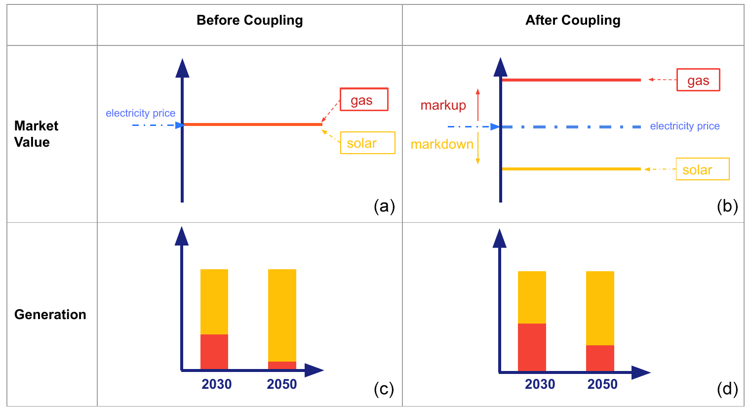
Figure 1Schematic illustration of the coupling approach for a simple power system in an IAM with coarse temporal resolution, consisting of only gas and solar generators (no storage). (a, c) Before coupling; (b, d) after coupling. (a, b) Endogenous prices (electricity price, market values of solar and gas generators); (c, d) endogenous quantities (generation mix). The markups (as part of a larger set of interfaced variables) are the differences between market values and electricity prices and are given by the PSM of high temporal resolution as price signals to the IAM. Usually, it is called a “markup” when the market value is higher than the annual average electricity price and a “markdown” if it is the other way around. For simplicity, in the rest of the text we only refer to “markup” and “markdown” collectively as “markup”, regardless of whether the market value is higher or lower than the average electricity price.
There are several advantages to this new coupling approach centered on linking prices. First, instead of simply prescribing quantities such as yearly generation and capacities, the approach allows endogenous investment decisions to be made by both models as they converge towards a joint solution. This gives maximal freedom to the coupled models while minimizing unnecessary distortions from one model to the other when some necessary quantities are being prescribed. Second, our coupling scheme provides an elegant treatment of both supply- and demand-side technologies using the concepts of market values on the one hand and capture prices on the other. Third, from a theoretical point of view, transferring the market values of all the generation types in a system alongside mappings of other relevant system parameters can lead to a convergence of the solutions of the two models under idealized coupling circumstances. It can be rigorously shown that our method contains an exhaustive list of interfacing parameters and variables for full model convergence of both quantities and prices. To the best of the authors' knowledge, the last point has not been explored or shown in any previous work.
In certain IAMs, VRE integration cost parameterization has been implemented to mimic the economic consequences of variability of VREs, especially when the models have a lower temporal resolution. Such VRE integration costs are contained in the uncoupled default REMIND power sector modeling. However, the exact parameterization always depends on a particular set of technological costs and parameters which might be subject to changes (Pietzcker et al., 2017), and the parameterization often needs to be carried out anew under new assumptions and scenarios. In contrast, the model-coupling approach is more general, and no such bespoke parameterization is needed.
Inspired by the theoretical framework based on the Karush–Kuhn–Tucker (KKT) conditions for power sector optimization problems (Brown and Reichenberg, 2021), we develop the theoretical basis for the coupling method in this section, which we use for validating convergence in numerical coupling in later sections. In Sect. 3.1, we analytically formulate the fundamental economic theory of the coupling approach. We first introduce the power sector formulations in the two uncoupled models (Sect. 3.1). Then we carry out a derivation of the convergence conditions and criteria, where we map the Lagrangians of the two power sector problems at different time resolutions and derive the equilibrium condition for the coupled models (Sect. 3.2). In Sect. 3.3, we introduce the iterative coupling interface which contains all the previously derived convergence conditions. For REMIND information being passed on to DIETER (Sect. 3.3.1) and DIETER information being passed on to REMIND (Sect. 3.3.2), we list and define the variables and parameters being exchanged at the interface as well as additional constraints and implementations which serve to improve the coupling.
Complete lists of the mathematical symbols and abbreviations can be found in the Appendices.
In the following sections, we first formulate the two uncoupled models and then move on to discussing coupled models. The theoretical tools we develop here are the foundation for the numerical implementation of coupling and serve to validate and assess the model convergence in the Results section.
3.1 Descriptions of uncoupled models
REMIND and DIETER are both optimization models. REMIND maximizes interannual global welfare from 2005 to 2150, whereas DIETER minimizes the power sector system cost for a single year and a single region. For a given REMIND Nash iteration (see Sect. 2.1), the single-region economy is in long-term equilibrium after the optimization problem is solved. Since, given a fixed national income, lower energy system costs mean higher consumption, which leads to increased welfare (see Appendix C for details), maximizing welfare can be assumed to correspond to minimizing energy system costs, a part of which is power sector costs. Therefore, to reduce the complexity of our analysis, we formulate an uncoupled REMIND model based solely on the power sector cost minimization and not the total welfare maximization. For the standalone REMIND, the multi-year power system cost for a single region equals the sum of all variable and fixed costs of generation,
where c represents the fixed cost for capacity, o represents the variable cost of running power generation, P denotes endogenous capacity, and G denotes endogenous generation (defined as including curtailment in REMIND). P and G are the decision variables of the problem. The sum in the objective function is over time index y and power-generating technology type s. The REMIND time index y stands for 1 representative year, which represents 5 or 10 years centered around it. So, even though the time step is 5 to 10 years, the time resolution is 1 year. For example, “y=2020” represents the years 2018–2022. Capital letters (both Latin and Greek) denote independent decision variables of the optimization problem. We classify an endogenous decision variable as independent if it is not uniquely determined by one or more other decision variables and has no binding constraints applied to itself that are not already accounted for by the constraints on the decision variable(s) it depends on. Note that, for simplicity, we treat all costs in REMIND in this formulation as if they are exogenous. In reality, REMIND has endogenous fixed costs due to technological learning as well as an endogenous interest rate. Some types of variable costs such as fuel costs are also endogenous and are determined based on primary energy balance equations for oil, gas and biomass. CO2 prices can also be endogenous under emission constraints.
Under the simplifying assumptions made for the derivation in this paper, the only independent decision variables are capacities, generations and curtailments. Small letters denote either exogenously given parameters or endogenous shadow prices.
For standalone DIETER, which has a year-long time horizon, the power system cost is
where is the endogenous hourly power generation (excluding curtailment – note that this is different from the generation variable definition in REMIND), h is the hourly index in a year from 1 to 8760, and s is the index for the power-generating technology in DIETER. is hourly curtailment, only applicable in the case of variable renewables vre (vre⊂s). Technology type s can be subdivided into two subsets: vre and dis (“dispatchables”). For simplicity, we abbreviate the index subscript from s|s=vre to vre and from s|s=dis to dis. Here, in order to differentiate from REMIND notations, we use overline to denote DIETER parameters and variables. Note that, for simplicity, in the derivation we treat the technology types in both models as identical, although in fact the technologies in the two models are not one-to-one mapped (Fig. B2). During the coupling all interface parameters and optimal decision variables need to be upscaled or downscaled when transferred from one model to the other.
The cost minimization of the total power sector cost Z and under constraints yields the optimal values of the decision variables, denoted as (, ) and (, , .
Without coupling, and under a baseline scenario, there are several constraints for each model. In the following equations we denote the shadow price (i.e., the Lagrangian multiplier) of a constraint by the symbol following ⟂. We use small Greek letters to denote endogenous shadow prices and small Latin and Greek letters to denote exogenous parameters. The major constraints are as follows (“c” stands for “constraint”).
- c1.
Constraint on generation for meeting demand, a.k.a. “supply–demand balance equation” or “balance equation” for short:
where dy denotes the annual REMIND power demand and denotes the DIETER hourly demand. The shadow prices (Lagrangian multipliers) λy and represent the annual and hourly electricity prices in REMIND and DIETER, respectively, and are equal to the marginal cost of one additional unit of electricity generation. αy,s is the annual VRE curtailment ratio in REMIND. Note that, technically speaking, REMIND electricity demand dy is determined endogenously, partially via competition with other energy carriers at the final energy consumption level, such as the competition between electricity and gaseous carriers such as natural gas or hydrogen in household heating. However, because here we have reduced REMIND to only intra-power sector dynamics for the purpose of mathematical analysis, we treat demand as exogenous.
- c2.
Constraint on maximum capacity by the available annual potential ψs in a region:
Note that the resource constraint in REMIND is only relevant for wind, solar and hydro and is assumed to be constant over the model horizon. Biomass availability is not modeled via a regional potential constraint. Instead, the availability of biomass is priced in through the soft-coupling to the land use model MAgPIE via a supply curve.
- c3.
Constraint on generation being non-negative:
Note that there are several other similar constraints on other positive variables such as capacities and curtailment. In practice, during the derivation they behave similarly to this positive generation constraint. Therefore, for simplicity, we do not include them in the derivation.
- c4.
Constraint on maximum generation from capacity:
where ϕy,s is the exogenous annual average capacity factor of the power plant s in REMIND in year y and is the exogenously given hourly theoretical capacity factor (i.e., before curtailment) of VRE in DIETER. Note that, strictly speaking, curtailments in the uncoupled REMIND and DIETER are endogenous decision variables but are not independent variables. However, here we use capital letters to denote hourly curtailment in DIETER as an independent decision variable to account for curtailment costs and other curtailment constraints that can arise from a more general formulation of the model.
- c5.
“Historical” constraints on capacities in REMIND. This makes REMIND a so-called “brown-field model”, i.e., a model accounting for the standing capacities in the real world. Past capacities (y< 2020) are “hard-fixed”; i.e., the variable capacities are fixed to certain numeric values. Current capacities (y=2020) are “soft-fixed”; i.e., the variable capacities are fixed to a corridor around certain standing numeric values: the lower bounds guarantee the already planned capacities, and the upper bounds reflect the finite physical capabilities of scaling up, defined by 5 % above the 2020 real-world data. For simplicity, we use only one constraint for both past and current capacities,
where py,s represents the standing capacities of technology s at time y in REMIND in the past and present years.
- c6.
Near-term upscaling constraint on VRE capacity expansion, represented by an upper bound on near-term capacity addition in model period , , where Δy is the REMIND model time step:
where qy,s is equal to twice the added capacity during the 2010–2020 period (only applied to Germany in the default REMIND).
Note that constraints (c5) and (c6) introduce interannual intertemporality into the power sector of REMIND. This additional interannual intertemporality determines that the model equilibrium can only be strictly satisfied across the sum of all the model periods and not for a single period. Another source of intertemporality in REMIND is the adjustment cost, which we ignore in the main text of this study since it introduces nonlinearity into the power sector and also plays a relatively small role in the overall dynamics.
Note that, regarding the simplification of REMIND above, to the best of the authors' knowledge, there is no theoretical or empirical concept that addresses the validity of drawing equivalence between welfare maximization and energy system cost minimization in IAMs. Naively, given that the gross domestic product (GDP) is unchanged, decreasing energy system costs raises consumption and therefore welfare. However, this is only valid under the assumption that energy is a substitute for (and not a complement to) capital and labor; i.e., one usually cannot raise economic output (GDP) simply by spending more on higher energy expenditure (while satisfying the same level of energy demand). Nevertheless, this is likely a necessary condition and not a sufficient one for proving the equivalence. More theoretical research will be needed to draw a precise and rigorous equivalence. However, in practice, we see that during our numerical calculation the model is well behaved according to this reduced theory, which means that the parameters in the models are in a regime where such an assumption is valid, at least in the case of IAM REMIND.
3.2 Economic theory of model convergence
In the last section we discussed the standalone uncoupled power sector formulations in REMIND and DIETER. In this section we discuss the coupled models and their convergence. Under simplified assumptions, we first derive the mapping between the models that is necessary for a convergence (Sect. 3.2.1 and 3.2.2), and then we derive theoretical relations that are later used to validate the numerical results of the coupled run (Sect. 3.2.3).
3.2.1 Derivation of convergence conditions
Our aim is to develop a method under which comprehensive convergence can be reached for soft-coupled multiscale models. We achieve this by deriving a mapping of the two problems such that their decision variables have identical optimal solutions and the endogenous shadow prices are also equal across the models. The convergence conditions of the coupled REMIND–DIETER model for the power sector are the result of such a mapping. Below, we first define what is meant by a “comprehensive model convergence” and then sketch the workflow of the derivation of a coupling framework which would result in a comprehensive model convergence of both decision variables and shadow prices. The detailed derivation is in Appendix D.
Here, we derive the conditions under which the endogenous decision variables are identical at each model's optimum, i.e., and – or, equivalently, pre-curtailment generation and . A convergence of the solutions of these two sets of annual decision variables for each technology s and for each year y, along with the convergence of shadow prices, gives rise to comprehensive model convergence. We show below that this can only be achieved if there is a harmonization at the level of the KKT Lagrangians of the two problems, following the methods first developed by Karush, Kuhn and Tucker (Karush, 1939; Kuhn and Tucker, 1951).
Our coupling approach fundamentally relies on mapping the parameterization of the Lagrangians for both optimization problems. It is trivial to show that, as long as the KKT Lagrangians are identical with respect to the decision variables, the solutions of the problem are identical, e.g., if an optimization problem A has Lagrangian and another problem B has Lagrangian , where x and y are decision variables of the optimization problems. Then, if we let , the two problems are identical, and they must have identical optimal solutions for the decision variables x* and y*. This is the basic logic behind the Lagrangian-based method. The challenge in the case of REMIND and DIETER is to show that when a decision variable representing the same physical quantity, for example, the annual power generation from a technology, is defined with low resolution in one problem and high resolution in another, there is nevertheless a viable mapping between the two Lagrangians. In this case, the parameterization of the Lagrangian is not only limited to exogenous parameters of the model, but also includes endogenous shadow prices and endogenous decision variables from the other model. Due to the endogenous nature of the latter two, the parameterization in the current-iteration model A must come from the solved results from the last iteration from model B and vice versa. Figure 2 illustrates the workflow of the analytical derivation of the convergence conditions.
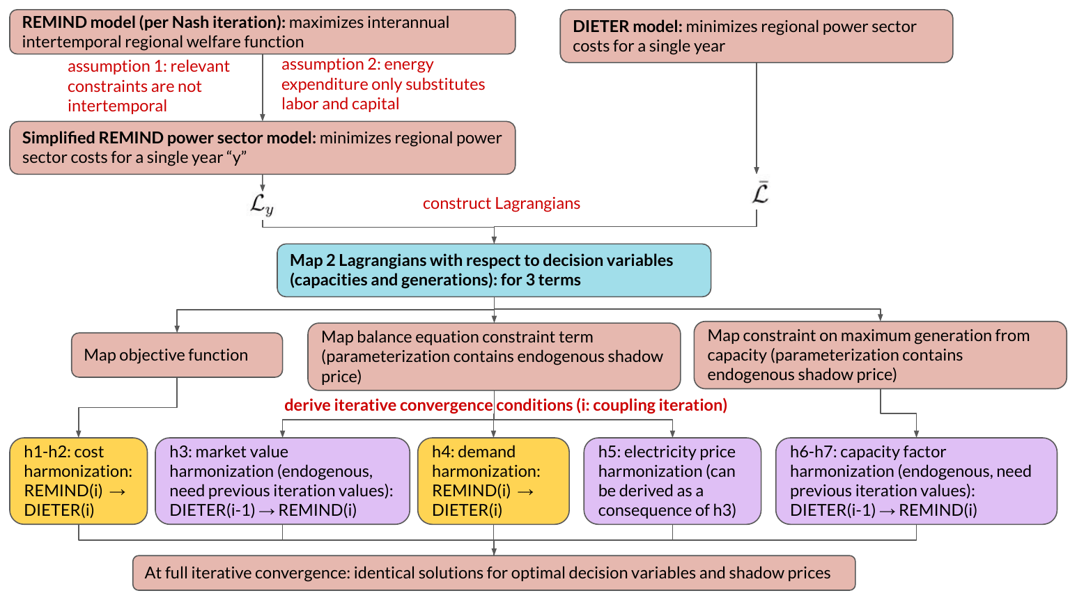
Figure 2The schematics of the Lagrangian-based derivation procedure for a simplified version of REMIND–DIETER iterative convergence. After simplifying assumptions, we can construct the Lagrangians of the reduced REMIND model and the full DIETER model for a single year (Eqs. 3–4). Comparing and mapping terms in the Lagrangians (a key step in bold), we discover that iterative exchange of a broad range of information is needed for a fully harmonized parameterization of the Lagrangians. Under the harmonization specified in the seven convergence conditions (color-coded for directions of information flow), the coupled models can give rise to identical optimal solutions of the models' respective (annually aggregated) decision variables and hence a full quantity convergence. The necessary shadow price convergence is shown in the detailed derivation of the harmonization conditions (h1–h7) in Appendix D.
The analytical derivation workflow, as shown in Fig. 2, is described in detail as follows. First, we apply simplifying assumptions to reduce the complexity of the uncoupled models (before the key step in blue in Fig. 2). Assumptions have to be made to justify reducing the scope of the REMIND model, such that for the purpose of the analysis it is on equal footing to DIETER. We achieve this by reducing the global REMIND model to a single sector (the power sector), single year and single region. To reduce the REMIND model from a macroeconomic–energy model to a power-sector-only model, we make similar assumptions to before when formulating the uncoupled REMIND power sector (see Sect. 3.1). To reduce the REMIND model further to a single year, we assume that the models only contain constraints in the power sector that are not intertemporal; i.e., we ignore the brown-field and near-term constraints for now. Since for each iteration of the REMIND model in Nash mode interregional trading happens between the iterations, the single-iteration optimization model is already for a single region and therefore does not require simplification. After these simplifying steps, in this part of the derivation, we can treat REMIND's power sector as “separate” from the rest of the model and treat the dynamics of a single year in REMIND as independent of the dynamics of other years. Later, the numerical results of the convergence can confirm to a large degree the validity of these assumptions, especially in the green-field temporal ranges, i.e., where the intertemporal brown-field constraints have little influence on the dynamics. Note that, with the inclusion of these intertemporal constraints in the derivation, the mapping becomes more complicated, especially for the near-term range, i.e., before 2035. So, in practice, this derivation of the coupling interface is only an approximation of what is needed for a full convergence of DIETER and REMIND, since it deliberately ignores such constraints. See also Sect. 6.1.
After the necessary simplification assumptions, we construct the Lagrangians for the simplified model REMIND and for DIETER (after the blue block in Fig. 2) (Gan et al., 2013). For a single-year reduced REMIND power sector model, the Lagrangian is
We would like to map it to the single-year DIETER Lagrangian :
The algebraic derivation of mapping the two Lagrangians term by term is presented in Appendix D. From this algebraic mapping, we can derive seven harmonization conditions (h1–h7) required for a full convergence. Conditions (h1)–(h7) are the subsequent basis for most of the information exchanged at the coupling interface. Among them, conditions (h3) and (h5)–(h7) (purple blocks in Fig. 2) indicate conditions which contain endogenous information that must come from the previous iteration of DIETER that is passed on to REMIND, such as markup and capacity factors. Conditions (h1)–(h2) and (h4) (yellow blocks) indicate conditions which contain information that comes from the previous iteration of REMIND and is passed on to DIETER. For schematics of the coupled iterations, see Appendix E.
This Lagrangian-mapping-based derivation can theoretically show that our approach (in its simplest form) necessarily leads to model convergence and has the advantage of being mathematically straightforward and rigorous. The necessary information from the power sector dynamics is all contained in the list of conditions derived from such a mapping. If the coupling contains less information, a convergence is not possible; at the same time, for a model convergence, one does not need to pass on any additional information beyond what is contained in this list of conditions. The list of information derived here is therefore complete and exhaustive for a coupled convergence.
3.2.2 List of convergence conditions
The convergence conditions (h1–h7), which are derived in detail in Appendix D following the procedure in Sect. 3.2.1, are summarized here.
- h1.
Annual fixed costs are harmonized: .
- h2.
Annual variable costs are harmonized: .
- h3.
Annual average market values for each generation type s are harmonized via markups from DIETER. We let denote the markup for technology s in year y in the last-iteration DIETER, i.e., the difference between the market value and the annual average price of electricity.
This is the heart of our coupling approach, using markups as the price signals. Intuitively, the markups represent the market value differences between REMIND and DIETER. The harmonization of market values is implemented by iteratively adjusting the market value for each generator type in REMIND to be the same as that in DIETER. As long as the market values (or per-unit-generation revenues) and costs are harmonized, the economic structures of the power market are identical and the models can converge.
Using markup Eq. (5), we modify the original objective function Z in the coupled version of REMIND by subtracting the product of markups and generations summed over all technologies and all years:
where Z′ is the modified REMIND objective function in the coupled version, and i is the iteration index of the iterative soft-coupling.
- h4.
Annual power demands are harmonized: .
- h5.
Annual average prices of electricity are harmonized:
where (i−1) indicates that the endogenous results are from the last iteration. This is shown in Appendix D to be a direct consequence of (h3) and (h4).
- h6.
Annual average capacity factors for each generation type s are harmonized:
where is the hourly capacity factor in DIETER, determined by endogenous hourly generation and annual capacities in the last iteration.
- h7.
Annual curtailments are harmonized:
In mapping the Lagrangians (Eqs. 3–4), except for the objective function, the rest of the parameterization contains endogenous shadow prices and endogenous quantities. Since endogenous values can only be known ex post, this imposes a strict requirement on the coupling that it must be iterative, with the endogenous part of the parameterization coming from previous iteration optimization results – usually from the other model. The mapping of the endogenous information requires careful argument in each case (i.e., the derivation of h3–h7). In the case of the balance equation constraint Lagrangian term (corresponding to c1), the shadow prices of the constraint in the current-iteration REMIND model are exogenously corrected by a set of technology-specific markups (see the introduction in Sect. 3.1), such that the new “corrected” market value in REMIND is manipulated to match the market value of the previous iteration of DIETER. This is the heart of our coupling approach using markups as the price signals. In the case of the constraint on maximum generation from capacity (corresponding to c4), the endogenous shadow prices in the current iteration REMIND can be shown to be automatically mapped to those in the previous iteration of DIETER given that the annual average capacity factors in the constraints are harmonized (h6–h7).
In actual implementation, most of the above mappings are modified for numerical stability (Sect. 3.3.2, Appendix H).
3.2.3 Theoretical tools for validating convergence
Here we first state the convergence criteria, which are mathematical relations that are being satisfied under model convergence. Then we also discuss equilibrium conditions of the coupled models that alongside the convergence criteria can be used to check numeric results to validate and assess the convergence outcome.
Under a theoretical full convergence of the coupled model,
- v1.
annual average electricity prices,
- v2.
capacities and
- v3.
(post- or pre-curtailment) generations
should all be identical at the end of the coupling in both models. These are the most important criteria by which we validate full model convergence. Technically, electricity price convergence (v1) (i.e., convergence condition h5) can be derived from (h3) to (h4). Nevertheless, we check this ex post, together with quantity convergence (v2–v3). In actual coupled model runs, following only the convergence conditions (h1–h7), the convergence criteria (v1–v3) might not be exactly fulfilled. Therefore, in practice, in order to validate the degree of numerical convergence, the alignment between REMIND and DIETER generation shares is set to be within a few percentage points before coupled runs terminate.
Besides using convergence criteria (v1–v3), we also use a type of equilibrium condition – the so-called “zero-profit rules” (ZPRs) – to validate the numerical model convergence. ZPRs are mathematical relations which state that, under market equilibrium, prices are equal to the costs for electricity. This is not always the case, especially in situations where there are extra constraints on the model that distort this equality. ZPRs contain model parameters and decision variables at market equilibrium, and they can be derived from the KKT conditions of the model (Appendix F). ZPRs are therefore reliable tools in ascertaining the sources of market values or the price of electricity of the power sector because, according to the ZPRs, one can always decompose the prices into the cost components, i.e., so-called levelized costs of electricity (LCOEs). The decomposition of prices into cost components is important because the prices of electricity in the power market are overdetermined by the energy mix, so it is possible that two different power mixes correspond to the same electricity price. In numerical results, a slight mismatch of the energy mix at the end of the coupling is unavoidable, so, alongside comparing the prices, it is often helpful to compare the makeup of the LCOEs across the models, such that they also appear harmonized at the end of the iterative convergence. Overall, ZPRs are a helpful tool for visualizing and understanding the power market dynamics, both from the point of view of each generator type and from the point of view of the entire electricity system. It is worth noting that the ZPRs, which are mathematical conditions derived from an idealized modeling of the power sector as fully competitive, are only an approximation of the real-world markets, where firm profits exist. ZPRs in their technical definition simply mean that, at model equilibrium, cost equals revenue. Given that the profits are defined as the difference between revenue and cost, the profits are zero in this situation. The name “zero-profit rule” therefore should not be overinterpreted beyond its technical contents, and one should be aware of its theoretical origin and the assumptions under which it is valid.
The ZPRs of the coupled model can be derived based on (1) the uncoupled models, (2) the modification made to the model due to the coupling interface (h1–h7) and (3) any additional modifications made to the model during our numerical implementation. In the last category, for a complete numerical implementation of the coupling, we add one additional capacity constraint, i.e., (c7) and (c8) for each model. The first capacity constraint (c7) is created in REMIND to circumvent the issue of extremely high markups from peaker gas plants in the scarcity hour of the year in the DIETER model, which otherwise causes instability during the iterative coupling. The second constraint (c8) is a simple brown-field constraint implemented in DIETER to address the fact that DIETER is a green-field model that is otherwise ignorant of standing capacities in the real world. For simplicity, (c7) and (c8) are not included in the convergence condition derivations in Sect. 3.2.1. The derivations of the ZPRs outlined by the above three steps have been carried out in Appendix F (uncoupled models), Appendix G (coupled REMIND only including the coupling interface, coupled DIETER including constraint c8) and Appendix H (coupled REMIND, including constraint c7).
In summary, the ZPRs for both coupled models are as follows.
- a.
Coupled REMIND
- i.
Technology-specific ZPR:
- ii.
System ZPR:
- i.
- b.
Coupled DIETER
- i.
Technology-specific ZPR:
- ii.
System ZPR:
- i.
The prime sign indicates that the term has been modified from the uncoupled versions due to implementation in the coupling. ν and ζ are capacity shadow prices introduced from the additional constraints (c7–c8) (Appendices G–H). It is worth noting that constraints (c7)–(c8) introduced due to coupling can impact the Lagrangians of the two models which we used to derive convergence conditions and criteria. However, in actual coupled runs, evidently there is only a moderate distortion due to these extra constraints. Condition (c8) even helps with convergence because it also puts most of the brown-field and near-term constraints which REMIND sees into DIETER (see Sect. 6.1).
Due to the fact that several sources of shadow prices cannot be incorporated during the derivation for convergence (Sect. 3.2.1), in numerical experiments of the coupled run it is appropriate to compare the following two types of prices across the two models for price convergence:
-
electricity price convergence, not including any capacity shadow prices;
-
sum of electricity prices and all respective capacity shadow prices converging.
Under the simplified analysis of convergence (discounting brown-field constraints, scarcity prices, etc.), price convergence in (1) is predicted by theory (see also convergence condition h5). However, this is only under the most idealized situation. Convergence in (2) on the other hand includes all the prices, which should match if LCOEs match across the system. We use the first type to check price convergence over iteration and use the second type only in the context of checking the system ZPRs across the models because of the theoretical relations between full prices and LCOEs.
3.3 Implementation via interface: exchange of variables
In this section we list parameters and endogenous variables that are exchanged between REMIND and DIETER. This already satisfies most convergence conditions, while the remaining condition (h5) is checked in Sect. 4 as part of the convergence criteria (v1–v3). An overview of the model coupling and the flow of information under convergence conditions is shown in Fig. 3.
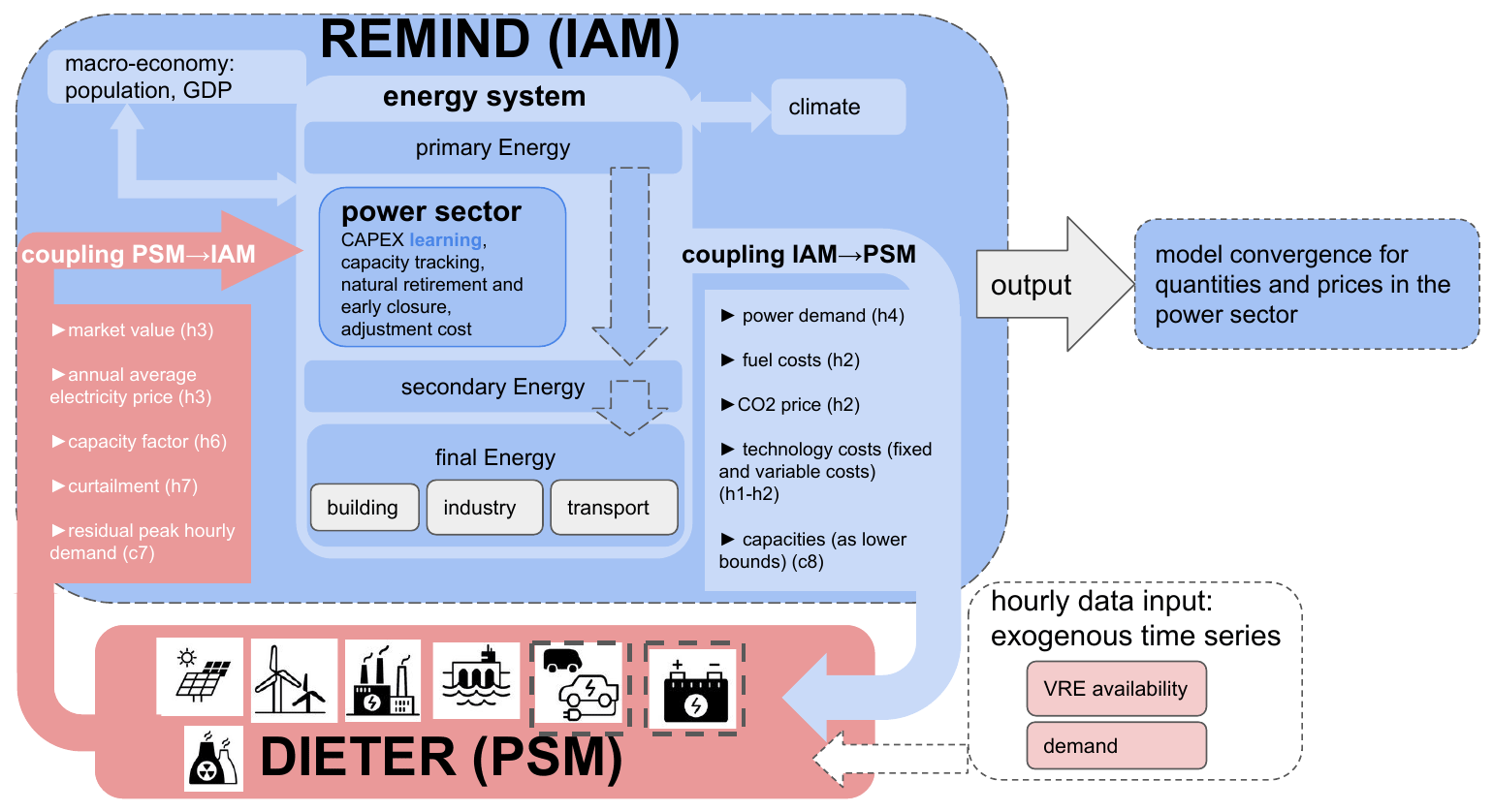
Figure 3The schematics of the REMIND–DIETER iterative soft-coupling. The power sector module of IAM REMIND, which is between the layer of primary-to-secondary energy transformation, is hard-coupled with other modules inside REMIND such as macro-economy, industry and transport. In PSM DIETER, the power market with generators of various types is modeled with hourly resolution, with options for storage and flexible demand. The information exchanged between the models (block arrows) is determined via the convergence conditions (h1–h7) derived before (Sect. 3.2.1). In order to improve performance and facilitate convergence, additional constraints (c7 and c8) are included in the coupling interface. The coupling interface for REMIND to DIETER is programmed as part of modified DIETER code and vice versa. Both interfaces are written in GAMS. For a single region, the scheduling of coupled iterations is illustrated in Fig. E1 in Appendix E. Sixteen DIETER optimization problems are solved for each representative year of REMIND in parallel, scheduled after each internal REMIND Nash iteration (see Sect. 2.1 for a description of the iterative Nash algorithm).
During the coupling, the following exchanges of parameters and variables take place iteratively in both directions via the interface.
3.3.1 REMIND to DIETER
The following information flow is from REMIND to DIETER.
-
Technology fixed costs (convergence condition h1)
- a.
Annualized capital investment cost: this is calculated from the endogenously determined overnight investment cost, plant lifetime and the endogenously determined interest rate. The overnight investment cost is determined from floor cost, learning rate and the endogenous global accumulated deployment. Note that investment costs decrease according to the endogenous learning rate. The interest rate is about 5 % on average but is endogenous and time-dependent in REMIND.
- b.
Annualized operation and maintenance (“O&M”) fixed costs (OMF): they are a fixed share of the capital costs.
- c.
Adjustment cost: this is technology-specific and is proportional to the capital investment cost. See Appendix I for its implementation.
- a.
-
Technology variable costs (convergence condition h2)
- a.
Primary energy fuel costs: they are endogenously determined as the shadow prices of the primary fuel balance equations in REMIND. Import prices, domestic prices of extraction, the amount of regional reserves and the amount of fuel demand can all influence the fuel cost. The relevant fuel costs include coal, gas, biomass and uranium. The fuel costs can have interannual intertemporal oscillatory components which can cause instability during iteration if coupled directly. We mitigate this by conducting a linear fit to the time series before passing them on to DIETER.
- b.
Conversion efficiency of each generation technology
- c.
O&M variable costs (OMV)
- d.
CO2 emission cost: an exogenous or endogenous CO2 price from REMIND multiplied by the carbon content of a type of fossil fuel and divided by the conversion efficiency of a generation technology gives the CO2 cost of 1 MWh of generation. Note that, in REMIND, biomass is considered to contain zero carbon emission when combusted.
- e.
Grid cost: in REMIND, the stylized grid capacity equation is proportional to the amount of pre-curtailment VRE generation. So, the grid cost is effectively a variable cost. Note that, in future work, grid costs can be modeled in more detail either in DIETER or in another PSM. Here, we use the parameterized grid costs which are implemented in the default REMIND as an approximation to the necessary grid cost.
- a.
-
Power demand (convergence condition h4). REMIND informs DIETER of the total power demand dy of a representative year y. In the next iteration of DIETER, the exogenous time series for the hourly demand from a historical year (2019) is scaled up to the demand of the last-iteration REMIND, dy(i−1), such that the annual total power demand in DIETER is equal to that of REMIND for each coupled year: .
-
Pre-investment capacities as an additional brown-field constraint (see constraint (c8) in Appendix G). ER is the endogenous early retirement rate in REMIND.
-
Total regional renewable resources for wind, solar and hydro (constraint c2), such that DIETER capacities are constrained by the same total available resources as in REMIND
-
Annual average theoretical capacity factors of VREs and hydroelectric ones in REMIND (convergence condition h6). We denote the pre-curtailment utilization rates of VRE capacity as “theoretical capacity factors”, as these can be achieved in theory if there is no curtailment. They are usually determined by meteorological factors such as wind and solar potential as well as the efficiency of the turbines or solar photovoltaic modules. In contrast, the post-curtailment utilization rates of VREs are “real capacity factors”, as these are the real utilization rates after optimal endogenous dispatch. The time series of theoretical utilization rates of VRE generations of 1 historical year in DIETER are scaled up such that the annual average theoretical capacity factors in DIETER equal the exogenous parameters in REMIND:
In DIETER, to be realistic, the rescaled hourly capacity factor for solar and wind has an upper bound at 99 %. The slight mismatch of the capacity factors due to this additional upper bound is negligible.
3.3.2 DIETER to REMIND
The following information is passed from the last-iteration DIETER to REMIND.
-
Market values are , and the annual average electricity price is (convergence condition h3), where is the annual average market value without the surplus scarcity hour price and is the annual average electricity price without the surplus scarcity hour price.
-
The peak hourly residual power demand is a fraction of the total annual demand (constraint c7). This produces the peak residual demand in REMIND dresidual,y that is proportional to the last-iteration DIETER peak to total demand ratio together with the in-iteration total annual demand dy(i):
where was defined in Appendix H (Eq. H1).
-
Annual capacity factors of dispatchable plants (convergence condition h6)
-
Annual solar and wind curtailment ratio: curtailment as a fraction of total annual post-curtailment generation (convergence condition h7)
For the information flowing from DIETER to REMIND, we use an innovative method of multiplicative “prefactors”, which can stabilize the coupling and increase the speed towards model convergence. The prefactors are automatic linear stabilizers of the current-iteration variables in REMIND. They depend on current-iteration endogenous variables in REMIND and are usually multiplied usually by the last-iteration endogenous DIETER results that are exogenously passed on to REMIND. This allows some degree of endogeneity in these exchanged variables, and their values can be adjusted according to the updated dynamics in the current REMIND iteration, such as interregional trading or price elasticity of demand, under which the exogenous last-iteration DIETER optimality can be used as an approximate starting point but does not necessarily hold exactly.
The prefactors usually depend on the differences between generation shares in the two models: for example, the prefactor for markup is a linear function of the difference between the current-iteration REMIND endogenous generation share and the last-iteration DIETER generation share. We illustrate the mechanism of prefactors using the markup for solar as an example: a lower market value for solar is consistent with a higher solar share according to the well-known self-cannibalization effect of a decreasing VRE market value as the VRE share increases (Hirth, 2018). Therefore, we can introduce an automatic stabilization measure through a negative feedback loop: if the REMIND endogenous share is larger than in the last DIETER iteration, in which case the in-iteration market value should be lower than the last-iteration DIETER market value, the multiplicative prefactor for the market value should be constructed such that it is smaller than 1. This lowers the market value for solar and decreases the in-iteration REMIND markup ηy,s(i), hence preventing over-incentivization of solar generation using the old market value based on the last-iteration energy mix. Overall, this produces a stabilizing effect on the system by making the markup as a price signal responsive to endogenous quantity change. We use prefactors ubiquitously when passing variables from DIETER to REMIND, such that during the iteration REMIND can adjust more smoothly and easily. We discuss the implementation of these prefactors in detail in Appendix H2.
In this section, we check the convergence behavior for prices and quantities (capacity and generation) in coupled model runs using the convergence validation criteria from the last section. Comparing the numerical results with the theoretical prediction, we can confirm that REMIND–DIETER soft-coupling indeed produces almost full convergence.
Throughout this section, we only use one scenario – a proof-of-concept baseline scenario. Under the proof-of-concept scenario of the coupled run, we disable storage (i.e., batteries and hydrogen) and flexible demand (i.e., electrolyzers) in both models, as this allows us to use the theoretically derived convergence criteria from Sect. 3, which would become overly complex in a model with storage and flexible demand. The coupled run is under a baseline scenario; i.e., there is no additional climate policy implementation. Since this is a configuration created only for comparison with the theoretical prediction, it is not meant to be a policy-relevant configuration. In more policy-relevant coupled runs, we turn on storage and flexible demand (see Sect. 5). For schematics and computational run times of the coupled iterations, see Appendix E.
For the coupled runs, we define a baseline scenario for the single region Germany under SSP2 assumptions corresponding to the “middle-of-the-road” scenario (for a definition of the SSPs, see Koch and Leimbach, 2023). Specifically, this means that REMIND runs for all global regions in parallel but that DIETER only runs for Germany. Only information in the German power sector is exchanged for the two models. We use a low CO2 price to represent “no additional policy”, which is USD 30 per tCO2 in 2020 and USD 37 per tCO2 for years beyond 2020. According to the 2011 Nuclear Energy Act of Germany, remaining nuclear capacities are set for early retirement in REMIND within the time period until 2022. We assume hydroelectric generation in Germany to come from running rivers. In DIETER, we cap the dispatchable generation's annual capacity factors at 80 % for non-nuclear power plants and at 85 % for nuclear power plants, so the dispatch results are in line with real-world power sectors. This constraint only adjusts the capacity factor constraint (c4), which would pose no additional distortion of our mathematical analysis.
Due to the particular implementation of offshore wind in REMIND, DIETER wind offshore capacities are fixed to those of REMIND to avoid too much distortion. Since in our scenarios offshore wind capacity in Germany is relatively small compared to other generators, this fixing represents only a minor distortion of the coupling. Hydroelectric generation in REMIND is assumed to have an average annual capacity factor of around 25 %. This capacity factor is implemented as a bound in DIETER. For simplicity, instead of a time series profile for hydroelectric generation, we allow the hourly capacity factor to be no higher than 90 %, meaning hydro is close to being dispatchable in all our scenarios. In the German context, hydro usually means run-of-the-river hydroelectricity, which has a variable output. Nevertheless, we find the 90 % maximum hourly capacity factor a reasonable assumption to make, since in our runs we do not yet consider pumped hydro as a technology in this study, so a more dispatchable quality of hydro can be assumed. Results presented in this section belong to the same coupled run under the proof-of-concept scenario.
4.1 Electricity price convergence
According to theoretical convergence criteria (under simplifying assumptions, Sect. 3.2.1–3.2.3), at numerical convergence, the electricity price of REMIND should be equal to the price of DIETER. However, REMIND is interannual intertemporal, whereas DIETER is only year-long, so we compare the differences over time as well as the interannual average of the price differences (Fig. 4).
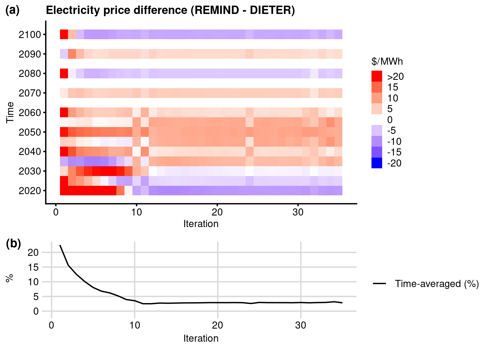
Figure 4Annual average electricity price convergence behavior of a coupled run for Germany under a “proof-of-concept” baseline scenario. (a) The difference between the annual electricity price time series of REMIND and the annual average electricity price time series in DIETER as a function of coupled iteration. (b) The interannual average of the differences in panel (a) as a share of the REMIND price. Due to the interannual, intertemporal nature of REMIND, in panel (a) the price difference can appear to have oscillatory components, obscuring the visual assessment of convergence. As a result, we show the trend of price convergence over iterations more clearly in panel (b) by taking the temporal average of the price differences. The REMIND price in both plots is a running average of three neighboring time periods to visually smooth out oscillations.
In Fig. 4a, the price difference oscillates from period to period. As the coupling starts, the REMIND price is much higher than DIETER, especially in the earlier years. After around the 10th iteration, the difference in the early years starts to reverse: DIETER's price becomes higher than REMIND. Around 2040–2060, REMIND has a higher average price than DIETER due to the VRE market values being higher than their LCOEs. This is discussed later in Sect. 4.3.2.
In Fig. 4b, we calculate the difference between two time series – the time-averaged power prices in the two models. We observe that the difference between them decreases over the iterations, showing a clear converging trend, and stabilizes at around 3 % of the REMIND price. There are two observations regarding the price convergence of the coupled run. First, the convergence happens rather quickly within 10 iterations. Second, the converged value of the price difference is not exactly 0 but is slightly above 0, a few percent of the full price (a few USD per megawatt hour). Under ideal convergence conditions, according to (v1), the two prices should be equal at full convergence for every coupled year. However, in practice, the average prices do not match perfectly, as there are several sources of distortions from capacity shadow prices. The capacity shadow prices come from many sources in both models: extra constraints such as (c7)–(c8) that are not part of the analysis leading to (v1), constraints that are in REMIND but not in DIETER (c5–c6), and exogenous wind offshore capacity in DIETER. Some of these capacity shadow prices in both models can be more or less consistent with each other (such as the standing capacity constraint in DIETER and brown-field constraints in REMIND), but others are not and can distort two models in different ways, causing some degrees of misalignment in prices. As discussed before, prices can be overdetermined by the energy mix (Sect. 3.2.3). Therefore, some of the capacity shadow prices – even though not aligned between the two models – can nevertheless cancel each other out (especially when averaged over time), potentially causing the price differences to be moderate. To examine exactly how well the prices at the end of the coupling match, we need to check the cost decomposition of the prices. This is discussed later in Sect. 4.3.
Also note that Fig. 4b presents a time-averaged price comparison, and on average the difference between the prices in the two models is small at the end of the coupling. However, when one compares the maximal deviation for any single year at the end of the coupling, it can be as high as USD 10 per megawatt hour, e.g., around 2050 (Fig. 4a). This is much larger than the 3 % averaged deviation in Fig. 4b. However, compared to default REMIND prices (which we cannot show due to limited space), we are fairly confident that the oscillation of the coupled REMIND results from internal dynamics that are also visible in the default uncoupled version. So, a time-averaged treatment is adequate in displaying the total price convergence here.
4.2 Quantity convergence
Besides price convergence, the capacity and generation decision variables must also converge within a certain tolerance at the end of the coupling. This is reflected in the generation mix (Fig. 5) and the capacity mix (Fig. 6) at the end of the coupled run. Due to the existence of several sources of mismatch between the two models already mentioned in the last section, which is already manifested in the mismatch in electricity prices of the two models, a certain degree of mismatch in quantities is also to be expected. Nevertheless, the agreement between the two endogenous sets of decision variables is satisfactory. For this coupled run, the differences of the generation share of any single technology between the two models are smaller than 4.4 % for each year until 2100. Figure 5b highlights some subtle model differences in generation. For example, after 2040, REMIND favors solar and coal, whereas DIETER tends to have more combined-cycle gas turbines (CCGTs) and wind onshore. Due to the low capacity factor of open-cycle gas turbines (OCGTs) and solar compared to the capacity factors of the other generators, the capacity mix differences between models are amplified for these two technologies (Fig. 6). However, overall, the generation mixes and the capacity portfolios at the end of the coupled run are generally similar.
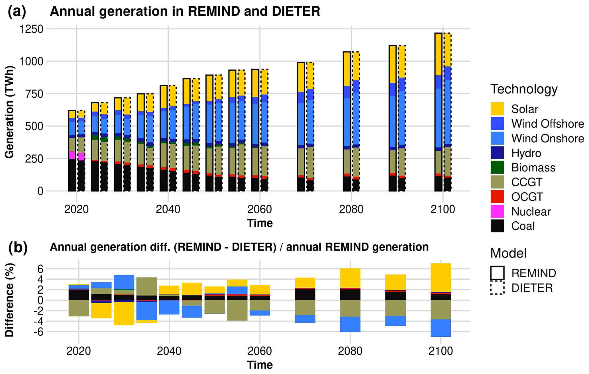
Figure 5Annual electricity generation convergence at the final iteration of a coupled run for Germany under the proof-of-concept baseline scenario. (a) Side-by-side comparison of the two generation portfolios at the end of the coupled run. (b) The difference between the generation mix in the two models as a share of the total REMIND generation.
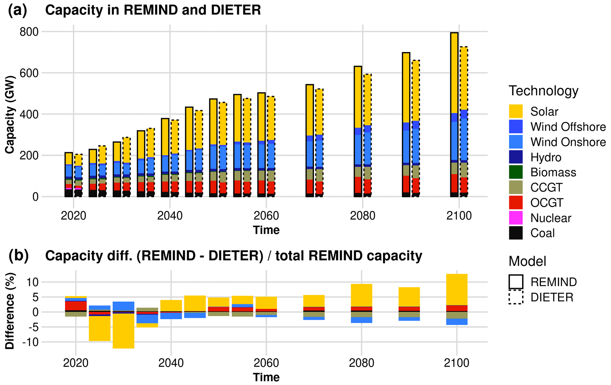
Figure 6Capacity convergence at the final iteration of a coupled run for Germany under the proof-of-concept baseline scenario. (a) Side-by-side comparison of the two models' capacity mix at the end of the coupled run. (b) The capacity difference between the two models as a share of the total REMIND capacity.
For periods that are policy-relevant in the short to medium term (i.e., before 2070), the convergence for quantities is generally slightly worse in the near term, i.e., in the 2020s and 2030s, likely due to the capacity bound mismatch in the near term (such as the capacity bounds c5–c6 in REMIND not being completely replicated by the standing capacity constraint c8 in DIETER). If DIETER does not contain identical bounds to REMIND, then its endogenous decision will have more of a green-field rationale than REMIND does, the latter of which is more constrained in the near term. In case an improvement in near-term convergence is desired, these bounds could be implemented more carefully and be more technology-specific. Due to the limited scope, we only apply a generic standing capacity constraint (c8) in DIETER to represent the basket of various constraints. The convergence of quantities is also not perfect in the green-field periods, such as after 2040, when both models are less constrained by near-term dynamics. The reason for this is likely the fact that, in DIETER, hydroelectric generation is not economically competitive against other, cheaper forms of generation such as solar and wind. However, in REMIND it is economically competitive, likely due to the long lifetime of the plants. Semi-exogenous wind offshore capacities in both models could also play a role. This is discussed in more detail in Sect. 6.1.
4.3 Zero-profit rules for the coupled model
As our analytical discussion showed before in Sect. 3.2.3, model equilibria in the form of ZPRs are useful for validating convergence in a more detailed way by decomposing prices into cost components as well as any perturbation from capacity shadow prices. In this section, we first compare the system LCOEs, price and capacity shadow prices of the two models for ZPRs on the system level, and then we show the technology-specific ZPRs. Using this validating step, we can visually ascertain that the cost components and prices or market values in the two models are remarkably similar on the system level as well as on the technological level, demonstrating that the underlying principle behind the coupled convergence holds to a good degree.
4.3.1 System-level zero-profit rule
At the convergence of the soft-coupled model, we expect ZPRs to be satisfied for the two systems individually (Eq. 11 for REMIND and Eq. 13 for DIETER); i.e., each price time series also matches the LCOE time series to a good degree, barring distortions from the capacity shadow prices. This is to say, under full convergence, that the time series of system LCOEs and the sum of the time series of the electricity prices and time series for capacity shadow prices for both models should overlap one another within numerical tolerance. The costs and prices at the last iteration of the coupled run are summarized in Fig. 7. The electricity prices derived from the shadow prices of the balance equations are shown in dark grey: (a) REMIND electricity price λy and (b) DIETER annual average electricity price . Adding all the sources of capacity shadow prices, we obtain the blue lines: (a) REMIND capacity constraints (c5–c7) and (b) the DIETER capacity constraint (c8). All capacity shadow prices have been converted to per energy unit via capacity factors. (Note: Fig. 4 shows the difference between the black lines without considering the capacity shadow prices. See Sect. 3.2.3.)
From Fig. 7, we can conclude that the ZPR for DIETER is satisfied to very good accuracy for every year (the blue line: the sum of the electricity price and the capacity shadow price has exactly the same value as the sum of the LCOE bars). For REMIND, the ZPR is satisfied year on year to a lesser degree but on average to a good degree given the interannual fluctuations. The prices in the coupled REMIND become very erratic for the early years (2020–2025), likely due to the interaction between the historical or near-term bounds in REMIND and the exchanged information from DIETER for those years. The LCOE component structures match well across the models for most years, which serve as additional visual support for the price convergence shown in Fig. 4; i.e., the cost structures behind the prices are harmonized as well at the end of the coupling. The origins of the differences between LCOEs and prices as well as the degree with which capacity shadow prices account for them can be found when one examines the LCOE and market values of specific technologies, which are analyzed next.
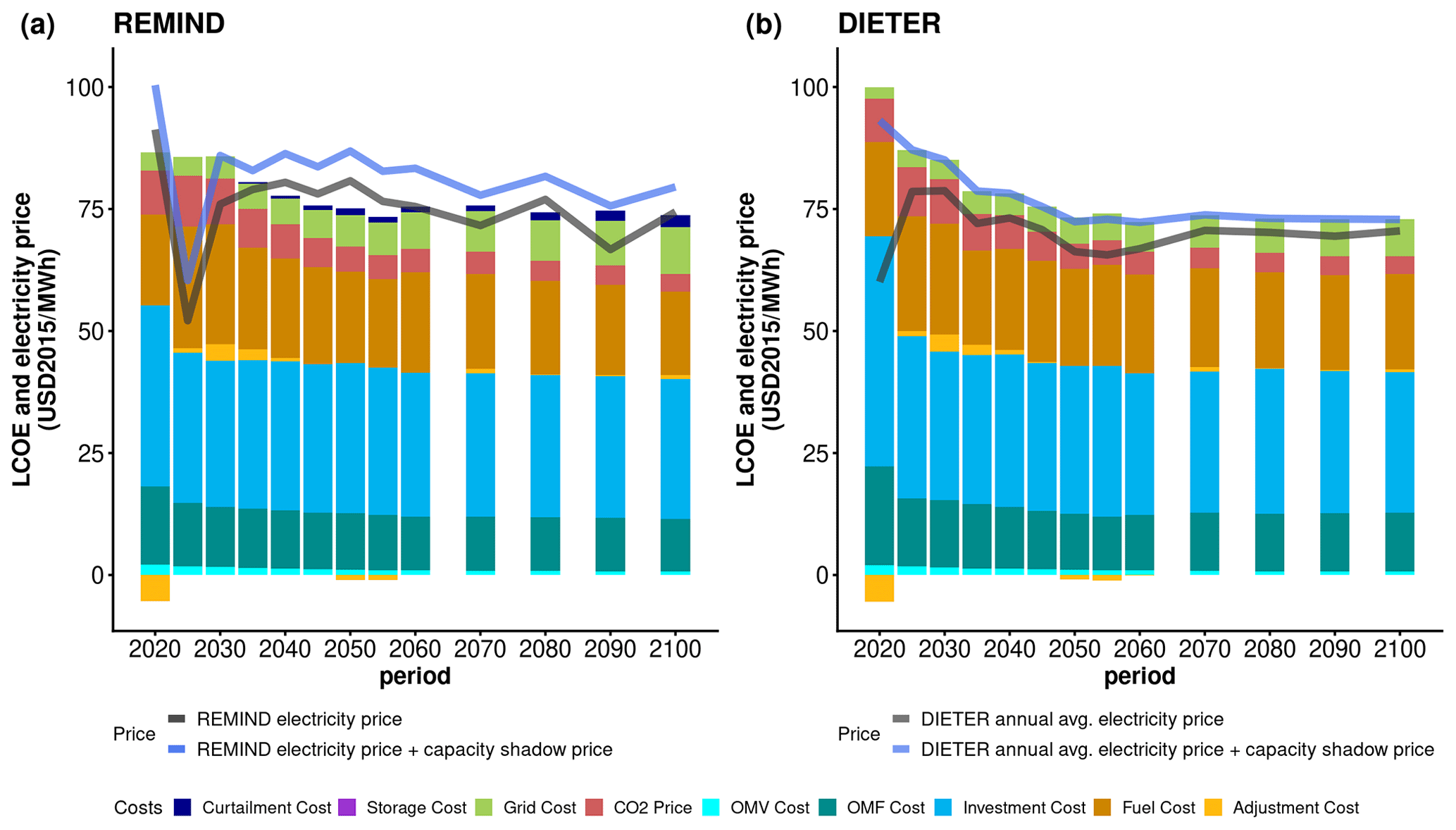
Figure 7Cost components of the system LCOEs (bars), electricity prices (grey lines), and the sum of electricity prices and capacity shadow prices for (a) REMIND and (b) DIETER under the proof-of-concept baseline scenario. Visually, the ZPRs for both models are satisfied within numerical tolerance. The intertemporal structure of the LCOE breakdown is very similar for most of the coupled periods. For DIETER, a small remaining difference exists between the price (grey line) and the LCOE (bars), which can be entirely explained by the capacity shadow price due to the standing capacity constraint. The REMIND price time series is a rolling average of three time periods. The large negative adjustment costs in 2020 are due to coal and nuclear phase-out.
4.3.2 Technology-specific zero-profit rules
After validating ZPRs on the system level, we further dive into each technology and check the ZPRs for each technology in both models at the last iteration of the coupled run (Fig. 8).
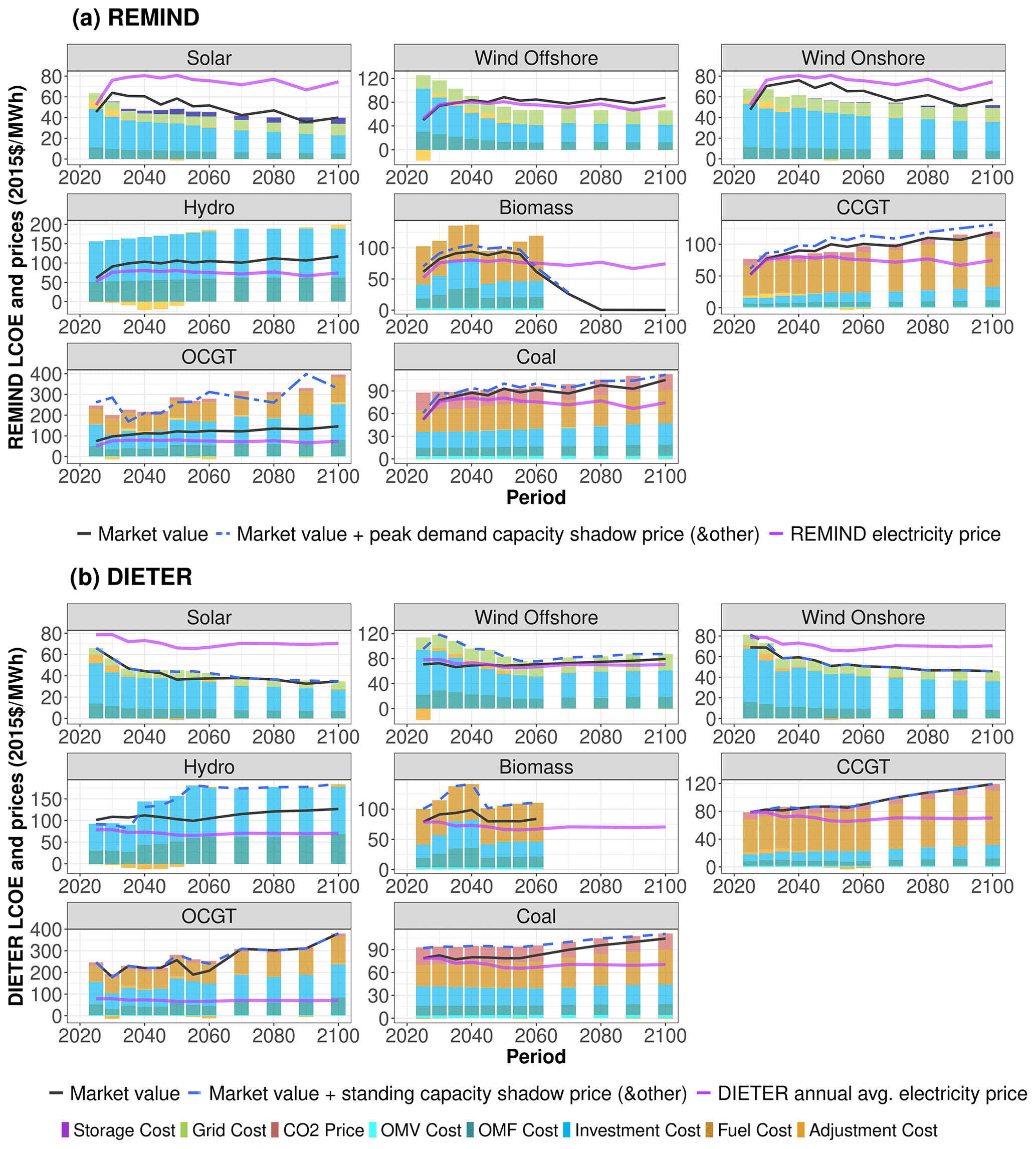
Figure 8Technology-specific costs and market values for (a) REMIND and (b) DIETER under the proof-of-concept scenario. Cost components of the technology LCOE are plotted in stacked bars. Market values are shown in solid black lines. The sums of market values and all sources of capacity shadow prices are shown in dashed lines: for DIETER (two-dash blue lines), they contain mostly the standing capacity shadow price and to a small extent the capacity shadow prices of the resource constraint; for REMIND (dashed blue lines), they contain mostly the peak demand capacity shadow price and small capacity shadow prices due to brown-field and resource constraints. Electricity prices are shown in purple solid lines as references. Due to large positive shadow prices in 2020 due to fixings to the historical capacities, only periods beyond 2020 are shown. REMIND market values and capacity shadow prices are a rolling average of three time periods.
In Fig. 8b, DIETER LCOE and market values for the eight types of generators are shown. As expected from the ZPR, the LCOE always matches the sum of the market value and capacity shadow prices for each technology and for each year (Eq. 12). The differences between the dashed and solid lines are largely the generation capacity shadow prices. It is worth noting that, at the end of convergence, the sizes of the shadow prices are in general small for the main generator types, e.g., solar, wind onshore, CCGTs and OCGTs. This indicates the fact that, for these technologies for most periods, the optimal DIETER generation mix is close to that of a green-field model. That is, DIETER hardly faces any exogenous constraints (except resource constraints that are aligned with those of REMIND) and can make fully endogenous investment and dispatch decisions based on cost information alone. On the whole, DIETER at the coupled convergence experiences only a small amount of distortion from the brown-field model REMIND, especially concerning the “model-suboptimal” real-world standing capacities from biomass, hydro and coal.
In Fig. 8a, we show the REMIND LCOE and market values for the same generation technologies. Due to the intertemporal nature of REMIND, the sum of the market value and the capacity shadow price for each technology and for each year generally matches the LCOE slightly less well than DIETER. This means that for REMIND the ZPR (Eq. 10) for each generator type is also satisfied to a good degree for the main generator types, e.g., solar, wind onshore, coal, CCGTs and OCGTs. The mismatch in biomass and hydro might come from the shadow price from historical capacities.
Since the differences between market values and costs are accounted for by the capacity shadow price to a large degree, it is worth interpreting physically the sources of these “hidden” costs and revenues. For REMIND, the capacity shadow prices consist of those in (c2), (c5) and (c6) as well as the “peak residual demand constraint” from DIETER (c7). Constraint (c7) is created to circumvent high markups, especially from peaker gas plants (Appendix H1), because peaker gas plants generate power mostly only at hours with high prices (especially the scarcity hour price) and therefore have very high market values compared to the annual average electricity price. The high market values of OCGT – usually more than 5 times the average annual electricity prices – act as a large incentive in the next-iteration REMIND and lead to over-investment in capacities. Over iterations, this causes oscillations in the quantities and prices in the coupled model and prevents model convergence. To circumvent the issue of high markup, we implement (c7) as an equivalent peak residual demand constraint. As can be shown mathematically (Appendix H), (c7) generates essentially the scarcity hour price, and it is very easy to validate this for OCGT in Fig. 8a. The capacity shadow price derived from this peak residual demand constraint, when translated to energy terms and added to the market value, correctly recovers the LCOE for OCGT, recovering the original ZPR (Appendix H1.2). This indicates that, under multiscale model coupling, an extra constraint is an effective way of circumventing potential issues of numerical divergence due to the large impact from short-term dynamics, such as the large market value of peaker gas plants.
For DIETER, the two sources of the capacity shadow price are the total renewable potential limit (constraint c2 in Sect. 3.1) and the standing capacity constraint from REMIND (constraint c8 in Sect. 3.2.3). For the first type, the resulting capacity shadow price is a hidden “positive cost” from the perspective of the power user since endogenously DIETER would like to invest more but is limited by the natural resources available. An example of this first type is hydroelectric power between 2020 and 2035 due to the limited resource (run-of-the-river) in Germany. It is worth noting that, from the generator's perspective, the capacity shadow price from the resource constraint can be interpreted as an extra resource rent. The second type of capacity constraint originates from the standing capacity, and the latter is received by DIETER from REMIND as a lower bound. This constraint usually results in a hidden “negative cost” from the perspective of a power user; i.e., a part of the cost (LCOE) does not get passed on to the electricity price, so the users get part of the capacity “for free”. (This can also be interpreted as subsidies for generators to sustain these unprofitable capacities.) This is because, based on green-field cost optimization, DIETER endogenously would invest less in certain technologies. However, since the standing capacities account for the existing generation assets in the real world, which can be model-suboptimal, the overall costs are above a green-field equilibrium and above the prices the user pays. We find examples of such a capacity shadow price manifested in biomass, coal and hydroelectric, all of which are part of the existing German power capacity mix, but evidently not all of them for any given period are “green-field optimal” based on the pure cost consideration in DIETER. Interestingly, after 2035, the sign of the capacity shadow price for hydroelectric generators reverses. This is likely due to the continuous decline in the VRE costs after 2035 tipping the power sector into a regime where hydroelectric becomes less economically competitive in DIETER, at least compared with REMIND. As a result, the standing constraint from REMIND starts to be binding on the capacity from below, relieving the resource constraint binding from above.
For DIETER, the capacity shadow price from the standing capacities also indicates the degree of disagreement between DIETER and REMIND. For most future years, REMIND standing capacity constraints are not binding in DIETER for solar, wind onshore, CCGTs and OCGTs, indicating good agreement between the models. The small amounts of shadow prices near 2060 for OCGTs and solar in Fig. 8b are likely due to the time step size change in REMIND which causes a small jump in the interest rates near these years.
Lastly, in Fig. 4, we observe a slightly higher average electricity price in REMIND than in DIETER, especially in the intermediate years. This could be due to fixed offshore wind capacities, which are never economical for endogenous investment in the parameterization used here. This generates a high capacity shadow price until around 2045–2060 that is visible in both DIETER and REMIND.
In this section, we present baseline and policy scenario results for Germany using a more realistic configuration of the coupled model with electricity storage and flexible electrolyzer demand for green hydrogen production, which is then used outside the power sector (e.g., in industry or heavy trucks). We show results for a baseline scenario and a net zero by the 2045 climate policy scenario. Note that, due to REMIND's global scope, under the net-zero scenario we also assume a larger climate policy background of a 1.5 ∘C goal for end-of-century temperature rise globally (corresponding to 500 Gt of the CO2 emission budget until 2100) and a larger regional goal of EU-wide net-zero emission. Both scenarios consider nuclear phase-out law in Germany.
In Sect. 5.1, we present long-term power sector development. In Sect. 5.2, we present short-term power sector hourly dispatch and price results. In the following, we broadly describe how these additional features are implemented.
-
Storage: we use a simple storage implementation where DIETER makes an endogenous investment in two kinds of storage technologies:
- 1.
lithium-ion utility-scale batteries;
- 2.
on-site green hydrogen production via flexible electrolyzers, storage and combustion for power production.
The principle of the coupling remains mostly unchanged. REMIND receives the price markups from generation technologies as in the case before without storage. However, for simplicity, the capacities of storage are not part of endogenous investment in REMIND. In REMIND, the energy loss due to storage conversion efficiency is taken as a fraction of the total demand from DIETER as a parameter and stabilized with a prefactor for each type of renewable generation (similar to the case of the curtailment rate in Sect. 3.3.2, point 4). Our battery cost development is given in Sects. S1–S2 in the Supplement.
The reason we only allow DIETER to endogenously invest in storage technologies is that the additional intertemporal optimization offered in REMIND is relatively less important than that for the investment of generation technologies. In REMIND, intertemporality mainly accounts for two aspects in the real world: (1) implementing adjustment cost and (2) tracking standing capacity. The adjustment costs simulate system inertia to rapid capacity addition or removal. In the case of battery and other storage technologies, the ramp-up of deployment faces relatively less inertia compared to wind and solar. Compared to generation technologies such as wind and solar, the storage technologies tend to have lower total capacities, meaning their ramp-up rate is usually lower. Also, their deployment is mostly constrained by their higher cost. For utility storage technologies, they are mostly not yet deployed at scale, which means that there is very little existing capacity and the investment in storage in REMIND is mostly green-field, rendering it unnecessary to give DIETER a standing capacity of them.
- 1.
-
Flexible demand: as a simple representation of flexible demand, we choose to implement a common power-to-gas (PtG) technology, i.e., the so-called “green hydrogen” electrolysis. We split the total power demand required to produce green hydrogen from REMIND from the total power demand dy(i−1) (Sects. 3.3.1 and 3.3.3) – both demands are endogenous in REMIND. We implement the electrolysis demand as completely flexible in DIETER, i.e., no ramping cost or constraint, thereby flexibilizing part of the endogenous total power demand dy(i−1) in REMIND. As a result, the cost minimization in DIETER automatically allocates the flexible demand to hours where electricity costs are low due to the existence of low-cost VRE. The economic value of flexible demand can be quantified by the capture price. The annual capture price of demand-side technology sd is the annual average price of the hours when the flexible demand consumes electricity, weighted by the hourly flexible power demand by electrolyzers: .
This concept is equivalent to the market value for a variable or dispatchable generator but here for a flexible or inflexible demand source. Similarly to before, we implement a stabilization measure using a prefactor (Appendix H2, point 5).
5.1 Long-term development
This section presents scenario results of the coupled model with a long-term view of capacity and generation using either the proof-of-concept scenario or more realistic configurations.
5.1.1 Baseline scenario
In Fig. 9a, under the baseline scenario, and with available storage and flexible demand, we observe a more than 35 % increase in the total power demand from 2020 to 2045 and more than 65 % by 2080. This is due to an increase in end-use electrification. The increased electrification comes from a moderate growth in electricity use in the building sector and a more significant growth in the electric vehicle (EV) fleet. In the building sector, the final energy share of electricity is projected to increase from 28 % in 2020 to 39 % in 2045. The final energy share of electricity in the transport sector is 22 % by 2045, up from 2 % in 2020. Note that, even under no additional climate policies, based on only the increase in EVs shares in new-car sales in many world markets today, we expect higher power usage from EVs in the future. Within the energy mix, we see a slow decline in coal generation over time, which is replaced by CCGT generation and a significant increase in VREs. The VRE share reaches above 50 % by 2045, but slightly less than half of the energy mix still contains coal and gas power. In terms of capacity expansion (Fig. 9b), due to both a lower generation cost and a higher power demand, solar capacity expands by almost 5 times from today until 2045. However, the moderate VRE shares mean that the requirement for battery capacity is not high, i.e., only 12 GW of batteries by 2045. Due to the low CO2 price, long-term electricity storage through hydrogen does not appear to be economically competitive and is not invested under the baseline.
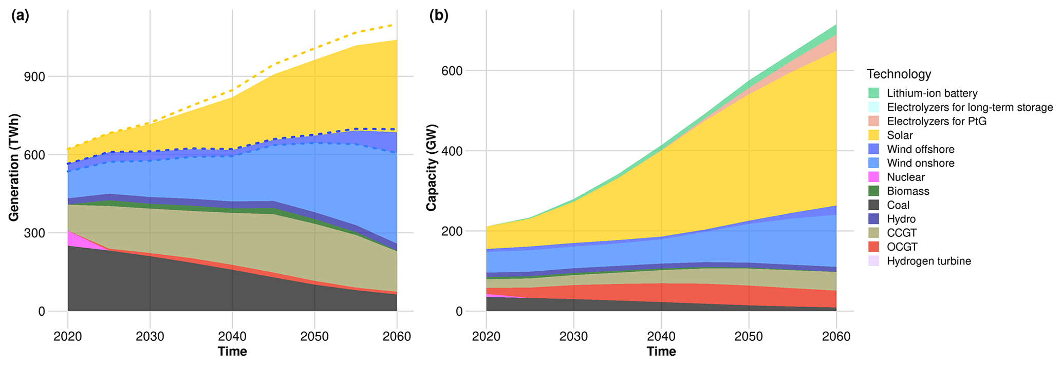
Figure 9DIETER–REMIND converged results of the long-term (a) generation and (b) capacity expansion for Germany's power sector in the baseline scenario, assuming a constant USD 37 / tCO2 CO2 price. Dashed lines represent generation before storage loss and curtailment. Storage generation is not visualized in panel (a).
By comparing the above baseline scenario (with storage and flexible demand) (Fig. 9) with the proof-of-concept baseline scenario (without storage or flexible demand) before (Figs. 5 and 6), it is clear that, while battery storage and partial demand flexibility play a role after 2040 in increasing the VRE share in Fig. 9, in the near term, the scenarios with and without available storage and demand flexibility look very similar under no additional climate policies. However, due to the technological learning effect, an even absent additional CO2 price policy, the energy mix here has a relatively high VRE share (> 60 %) after 2050 compared to the basic case without storage and demand-side flexibilization. However, due to the low CO2 price there is still a significant share of dispatchable technologies such as CCGTs and OCGTs, which is more economical than the implementation of long-term power storage via electrolysis and hydrogen turbines.
5.1.2 Net-zero policy scenario
In Fig. 10, under a stringent climate policy (economic-wide carbon neutrality in 2045), with available storage and partially flexibilized demand (for hydrogen production used in other sectors), the total power demand more than doubles, and the power mix is dramatically transformed. Compared to both the baseline case without storage and demand-side flexibilization (Figs. 5 and 6) and the baseline scenario with storage and flexible demand (Fig. 9), a very high VRE share in the generation mix is reached already by 2040 (> 94 %). This is mostly due to an earlier investment in VREs to drive down the cost, combined with the increased deployment of both short- and long-term storage and flexibilization of part of the demand. Capacities for storage increase significantly: lithium-ion batteries from 18 GW in 2020 to 125 GW in 2045, and 37 GW of hydrogen electrolysis and hydrogen turbine capacity (with ∼ 40 TWh of H2 storage capacity). Despite high storage capacities, due to a high VRE share, curtailment and storage loss still increase quite significantly with time, especially for solar PV. However, note that in a coupled run where interregional transmission expansion is possible connecting Germany and the rest of Europe, this loss can be reduced (see Sect. 6.3). In terms of capacity expansion (Fig. 10b), gas power plants are mostly replaced, as hydrogen turbines fill the role of peaking dispatchable plants that guarantee supply for peak demand hours. The CCGT gas turbines are equipped with CCS.
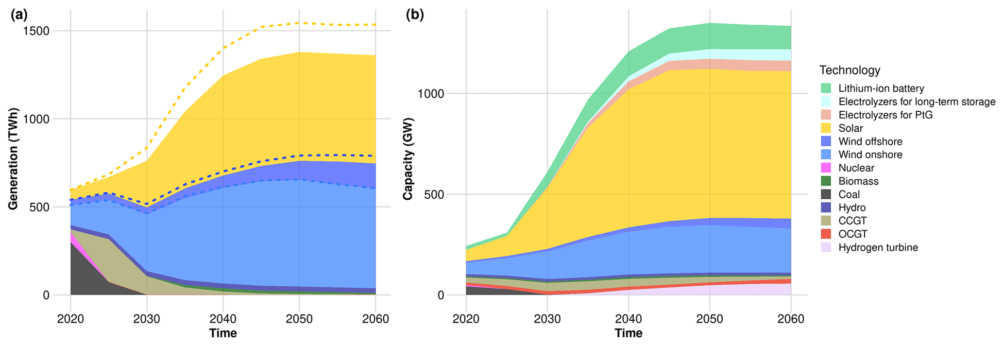
Figure 10DIETER–REMIND results of the long-term generation and capacity expansion for Germany's power sector in the “net-zero 2045” scenario. The CO2 price is endogenously determined based on the climate goal. It is USD 115 / tCO2 for 2030, USD 292 / tCO2 for 2035, USD 464 / tCO2 for 2040, and USD 636 / tCO2 for 2045. Dashed lines represent pre-curtailment generation. Storage generation is not visualized in panel (a).
Under the stringent climate policy scenario, dramatic changes in the end-use sectors will be under way in the form of direct electrification and substitution of fossil gas with hydrogen. In the building sector, the final energy share of electricity is projected to increase from 28 % in 2020 to 66 % in 2045. In transport, the final energy share of electricity will be 56 % by 2045. In the industry sector, the share of electricity increases from 25 % to 63 %. By 2045 there is also a notable increase in the use of green hydrogen produced from 45 GW flexible electrolyzers (at about 42 % of the average annual capacity factor), amounting to 0.5 EJ (3.5 million tons) per year in the final energy, which is primarily used in industry. For a comparison with other published German net-zero scenario results, see Sect. S4.
5.2 Short-term dispatch
In this section, results of hourly resolution are shown and discussed for a selected model year. We use established methods such as RLDCs to visualize the hourly dispatch result and show the hourly generation and dispatch time series for some typical days in summer and winter.
5.2.1 Residual load duration curve model comparison
RLDCs can be used to visualize the dispatch of energy system models. Each subsequent curve is calculated by subtracting the generation of a technology from the hourly residual demand curve and then sorting the remaining demand in descending order. On the left-hand sides of the RLDC graphs, one can easily check the amount of residual demand not met by variable wind and solar production. The topmost line in the RLDC graph is the load duration curve for inflexible demand (excluding the demand from flexible electrolysis for hydrogen production used in other sectors).
In a baseline configuration without flexibilized demand or storage, despite lacking the explicit hourly dispatch, via bidirectional soft linkage, REMIND was able to achieve a final dispatch result that replicates DIETER to a satisfactory degree (Fig. 11). This is a combined effect of a convergence of capacities (Sect. 4.2) and full-load hours at the end of the coupled run. In the peak residual demand hour (the leftmost point in the RLDC), the DIETER-coupled REMIND accounts for the requirement of dispatchable capacities via the constraint (c7), and the composition of the mix is replicated from DIETER and correctly guarantees that the peak hourly demand is met.
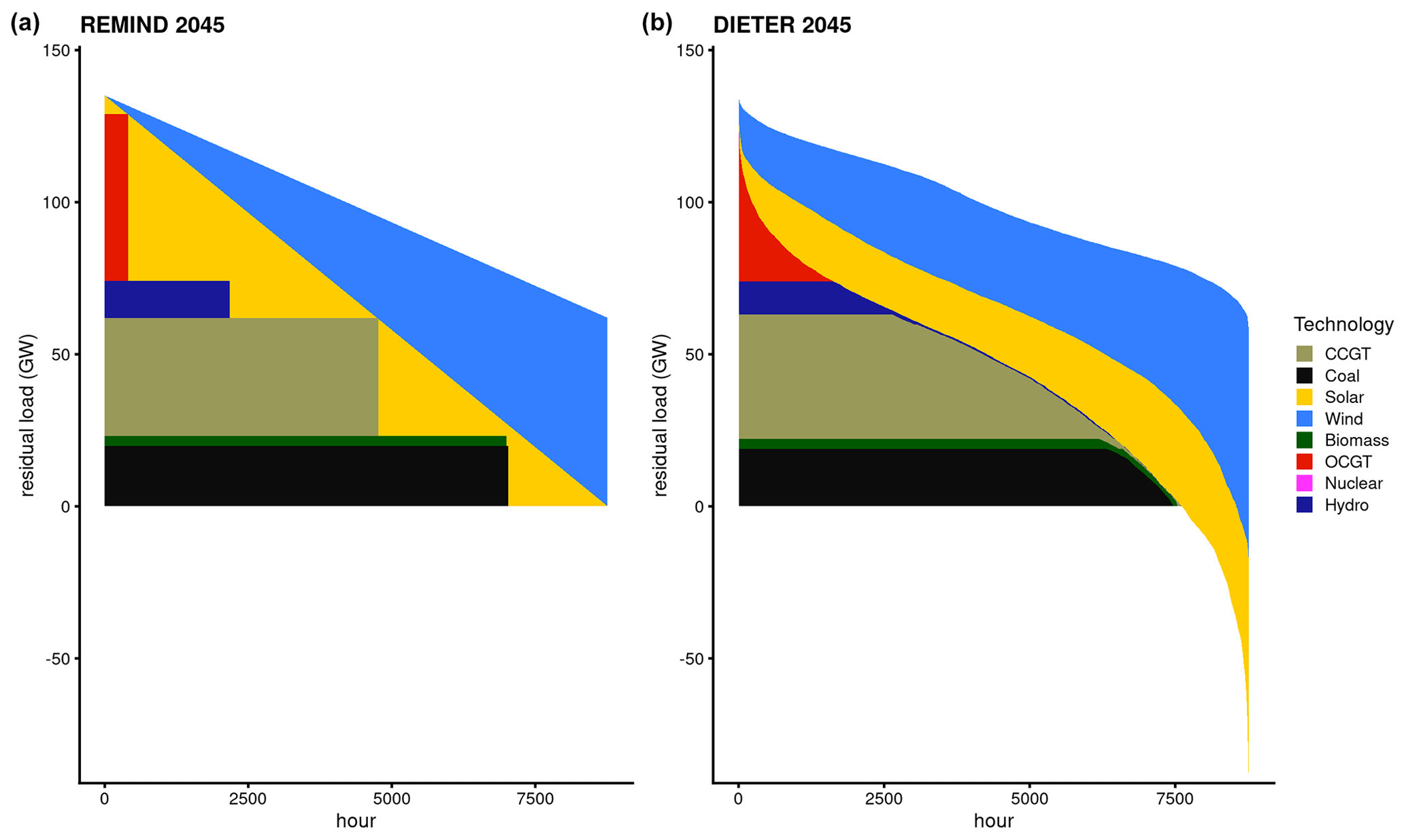
Figure 11Side-by-side RLDC comparison between (a) REMIND and (b) DIETER for the simple configuration under the baseline scenario without storage or flexible demand. The DIETER RLDC (b) is constructed by subtracting hourly generation from hourly load and sorting with dispatchable generation technologies plotted in order of their annual average capacity factors. VREs are arranged such that the generation with a higher curtailment rate (i.e., solar in this case) is on the inside of the graph. To construct the REMIND RLDC (a), the dispatchable generations are sorted by their capacity factors and stacked from the bottom. The rectangles depicting dispatchable generation are made up of the width equal to the full-load hour and the height equal to the capacity. The top-most lines on either side are load duration curves (sorted hourly demand, which is entirely inflexible under this setup). For the purpose of better visualizations, solar and wind RLDCs are tilted at an angle for REMIND and plotted in the same order as the DIETER RLDC. For simplicity, in REMIND wind and solar RLDCs share the same top pivot point in the peak residual demand hour.
In a net-zero policy with storage and flexible electrolysis demands, comparing dispatch results under both scenarios (Figs. 11 and 12) for the model year 2045, it can be observed that, under a stringent emission constraint, the system allocates a significant amount of short-term storage to replace the dispatchable generation such as coal and CCGTs. Long-term storage such as hydrogen electrolysis combined with hydrogen turbines further reduces the capacity factor of the remaining OCGTs and CCGTs. Besides storage, there is also a significant amount of deployment of flexible electrolysis demand for producing hydrogen (PtG) that is not used in the power sector but is in industry or heavy-duty transport. The use of PtG technologies leverages cheap variable wind and solar energy to achieve the goal of sector coupling. By way of storage and PtG, a significant share of the curtailment can be utilized (more than 70 %), either by shifting the supply to times of low VRE production via storage or by producing hydrogen using surpluses which can be used in other sectors.
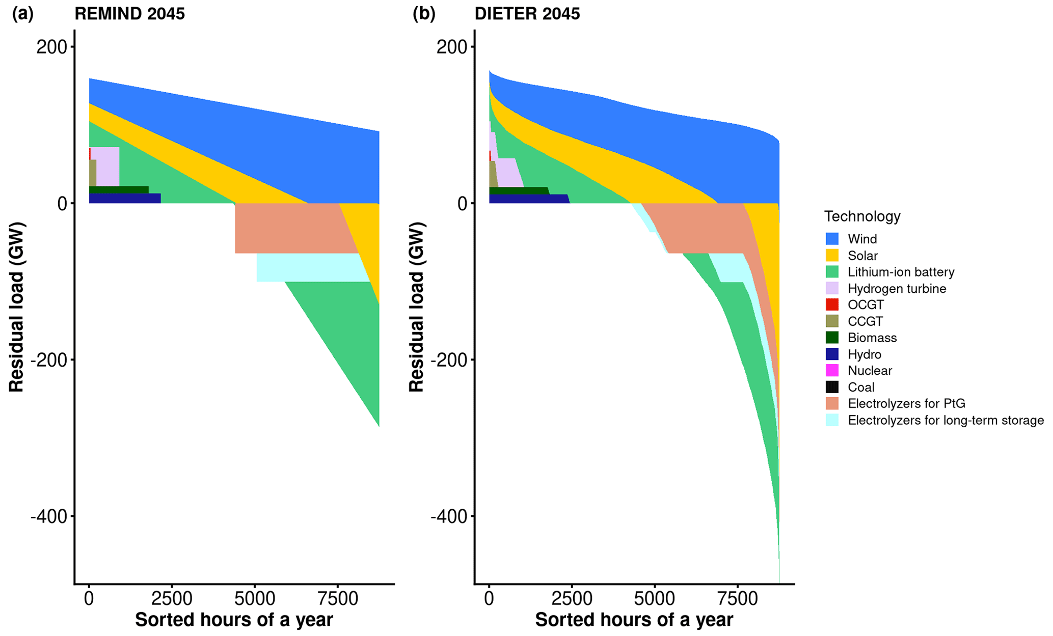
Figure 12Side-by-side comparison between the (a) REMIND and (b) DIETER RLDCs for the “net zero by 2045” scenario with storage and flexibilized demand for Germany. The storage loading and discharging in the DIETER RLDC (b) are constructed by subtracting hourly loading or discharging from hourly inflexible load and sorting. The REMIND RLDC (a) is constructed similarly to Fig. 11. The top-most lines on either side are load duration curves for inflexible demand. For better visual comparison, in REMIND the solar RLDC starts at 80 % of the peak residual demand.
5.2.2 Hourly dispatch and power consumptions for typical days in summer and winter
To more directly inspect the results of the hourly dispatch under various scenarios, we visualize the hourly generation and demand for typical days. Due to the climate in Germany, solar potential is particularly low during winter months. Therefore, it is important to observe the periods in both summer and winter.
From the optimal hourly dispatch results of typical days from the coupled model, we observe that, compared to the baseline (Fig. 13a–b), in 2045 for a net-zero year (Fig. 13c–d), there is a significant amount of surplus solar generation in the summer during the day and some amount of surplus wind generation in the winter during nights and days. Under a net-zero scenario, the generation from fossil fuel plants in the baseline is replaced by a battery dispatch (especially in summer) and hydrogen turbines (especially in winter), and the peaker plants, which under the baseline are turned on in the summer evening, are partially replaced by solar overcapacity and batteries. A significant share of renewable surplus energy is used for the production of green hydrogen – hydrogen made from zero-carbon electricity. Due to the complete flexibility of electrolyzers, the capture price of hydrogen production is only around one-third of the average price of electricity (Sect. S2 and Fig. S1 in the Supplement).
In winter, hydrogen turbines serve as a base load for the few days when wind generation is insufficient to meet the demand. To ensure supply during longer winter periods of “renewable droughts” with little wind and solar output, e.g., over a 2–3 d period (hours 540–600 in Fig. 13d), long-term storages with hydrogen electrolysis and hydrogen turbines and some dispatchable generation (such as CCGTs with CCS and an integrated biomass gasification combined cycle) play a major role.
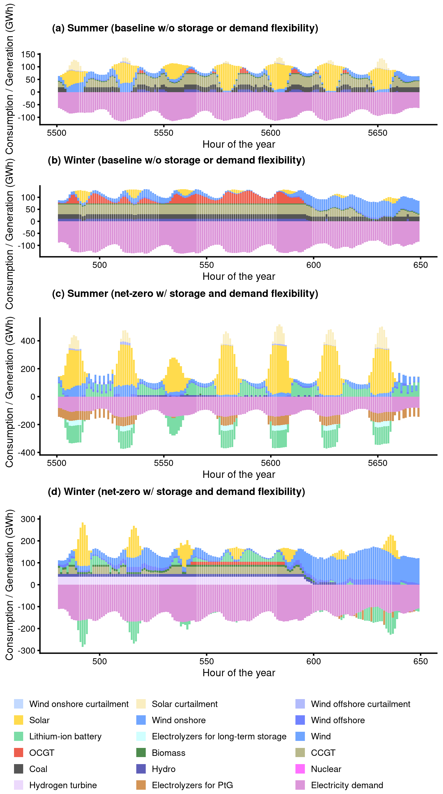
Figure 13Comparison of hourly generation (positive) and consumption or storage loading (negative) for a few consecutive typical days in two seasons in Germany in 2045. (a) Summer, under the proof-of-concept baseline scenario, no storage, or flexible demand. (b) Winter, under the proof-of-concept baseline scenario, no storage, or flexible demand. (c) Summer net-zero scenario with storage and flexible demand. (d) Winter net-zero scenario with storage and flexible demand. Due to the fact that modern electrolyzers are very flexible, no ramping costs are applied to them in the models, and therefore some switching behavior between PtG electrolyzers turning on and off can be seen, but this is a minor artifact.
In this section, we discuss the reasons for remaining differences between the coupled models as well as the assumptions and limitations of the soft-coupling.
6.1 Remaining discrepancies
In all our test runs, at the end of the coupling, it is always the case that the two models cannot be perfectly harmonized, and there is a slight residual difference in the convergence results (Sect. 4). The reason is two-fold.
The first reason is “legacy mismatch”, i.e., a mismatch in brown-field standing capacity constraints in the two models. The coupling method we develop here is mostly based on price information for achieving convergence. Therefore, capacity constraints that are present in the standalone long-term model but not in the standalone hourly dispatch model need to be transferred. These standing capacities are hard to evaluate purely based on economic terms, as they are ultimately a result of real-world actions and policies that might not align with the simplified economic incentives in techno-economic energy models. Therefore, the only way this information can be transferred from the brown-field model to the green-field model is by implementing a lower capacity bound in the latter. However, this bound nevertheless might not capture all the shadow prices caused by the standing capacities in REMIND. This is ultimately due to the specific generic form of the constraint we implemented: i.e., we pass on the pre-investment capacities as a lower bound regardless of the technology types. In general, hidden “legacy revenues”, which are manifested as the shadow prices of economically less competitive generators in DIETER, such as biomass, coal or hydroelectric (solid line lower bars in Fig. 8), provide incentives for brown-field models to deploy them over the long term but do not provide enough economic cases for the green-field model. This results in an observed phenomenon in the coupled run that, if these legacy capacities and their impact on the costs have not been fully transferred to the green-field model, the prices of the green-field model tend to be lower than the coupled brown-field models, causing distortion of the convergence of quantities. The effects of legacy mismatch and illustrative test run results are discussed in more detail in Supplement Sect. S3.
The second reason for the discrepancies at the end of the coupling is the actual mismatches in the Lagrangian harmonization itself, which can originate from multiple sources. It could be due to intertemporal constraints and dynamics (such as adjustment costs and brown-field constraints) not linearly reducible to single-year dynamics, resulting in misalignment between the multi-period REMIND and the single-year DIETER. It could also be due to slight numerical inaccuracies of the interest rate estimate that are not explicit in REMIND but that are derived from endogenous and intertemporal consumption. Lastly, there could be a mismatch due to a linear fitting of REMIND endogenous time series of fuel costs (biomass, oil, coal, uranium) before passing this information on to DIETER, which might result in a small amount of mismatch for fuel costs between REMIND and DIETER.
6.2 Limitations of the coupling methodology
There are limitations to our proposed methodology in terms of both convergence of two multiscale power sector models and other potential applications of model convergence. Firstly, in terms of the problem presented here – a multiscale power sector model coupling –, the method derived here is only necessary for a full convergence but may not be sufficient; i.e., a full convergence is not guaranteed. A number of additional factors could prevent a full convergence. One is the legacy mismatch and misalignment in Lagrangian mappings mentioned above in Sect. 6.1. Another factor is the role prefactors play (Sect. 3.3.2, Appendix H2). The prefactors help stabilize the coupling by turning exogenous values obtained from the last-iteration DIETER into endogenous values in REMIND, such that they can be adjusted to be in line with the optimal mix of the current iteration. However, they usually contain some small positive or negative parameters that are determined heuristically (e.g., in Eq. H13). These heuristic parameters usually come from rough estimates based on relations between variables in the system and generation shares, e.g., how much the market value of solar generation will decrease when the solar generation share increases by a certain percentage. In practice, while the prefactors help stabilize the run and improve the convergence speed, choosing the wrong prefactor parameters can lead to divergence or instability. Second, another limitation when it comes to modeling power market multiscale coupling is the number of products on the market. In the formulation here, both models describe the general equilibrium of a competitive market with one type of homogenous goods, i.e., electricity. However, if we introduce heat as a byproduct, such as from a combined heat and power plant, then there are two types of goods: heat and electricity. The feasibility of coupling models with more than one type of good or market has not yet been explored. Thirdly, there are multiple iterative processes that are internal to REMIND, which happens concurrently with the DIETER–REMIND coupled convergence. Among these processes, the DIETER and REMIND Nash algorithms (for interregional trading) both run between the internal REMIND Nash iterations, which means that they are external to the REMIND single-region optimization problems and therefore are soft-linked. Nevertheless, in our runs, we observe the power sector convergence to be rather swift and smooth and to happen in parallel to other iterative processes, such as the Nash algorithm and the CO2 price path algorithm (for climate policy runs). However, systematic monitoring of the multiple internal convergence processes in REMIND during the REMIND–DIETER convergence processes under other model setups and configurations is still to be more thoroughly researched. More generally, the approach developed here – the Lagrangian mapping method for converging two multiscale optimization problems – could be useful for a general modeling of market equilibrium of multiple time resolutions. In this study, the resolution in the coupled problems is specifically only meant for temporal resolution. However, mathematically speaking, coupling models of different spatial resolutions (or both temporal and spatial resolutions) should be very similar. At least in theory, the soft-coupling approach developed here should be applicable to increasing the resolution in any arbitrary independent/orthogonal dimension of the problem of finding equilibrium market dynamics. In theory, it is also possible to build a multi-layer coupled problem architecture, where at each level the low-resolution variables can be disaggregated into finer resolution along some dimensions. However, further research is needed to explore the feasibility and convergence performance of such schemes.
6.3 Limitation of coupled results
Since the nature of this study is a proof of concept, the scenario results presented should be primarily interpreted as such. Nevertheless, it may be useful to enumerate a list of limitations for a more accurate interpretation of the results.
-
The power sector is only coupled for one single global region; i.e., information exchange only occurs for the variables of one region, Germany, while all the other regions contain the low-resolution version of the power sector of the uncoupled REMIND. The former coupled one-region result is based on a time series of VRE production today in a world of low- to medium-VRE shares and a very limited power grid expansion (in 2019). The latter results of the uncoupled regions however are parameterized based on results from a detailed PSM under a more optimistic assumption of transmission build-out, which allows VRE pooling from an expanded EU-wide power grid to smooth out regional weather variations (Pietzcker et al., 2017). Note that, in the standalone REMIND, while by default there are no annual electricity import and export imbalances between countries and regions, transmission during the year is implicitly assumed, especially for the EU region. Comparing the capacity and generation mixes of the coupled and uncoupled runs (Appendix J), we find that, in the uncoupled case, there are slightly more solar and wind capacities and generations and much less gas generation in the long term. EU-wide transmission expansion would pool both supply and demand variability, thus reducing the need for dispatchable capacity for meeting the peak demand.
-
Due to the scope of this study, we implemented a limited set of options in storage and sector-coupling technologies in this study and neglected the additional supply-side details for the German power market (such as the reserve market). Many potentially significant technological options consisting of pumped hydro storage, compressed-air energy storage, vehicle to grid and flexible heat pumps are not explicitly modeled.
-
Ramping costs for dispatchable generators are not considered, although the effect should be small (Schill et al., 2017).
-
In terms of power transmission and trading inside Germany, we assume a very simple “copperplate” spatial resolution, not explicitly modeling transmission bottlenecks inside the region. Currently, the grid capacity equation is parameterized to be proportional to pre-curtailment variable renewable generation, and the parameterization is rather optimistic based on PSM studies conducted in Pietzcker et al. (2017). As hinted at in a recent work by Frysztacki et al. (2022), the lower level of spatial detail results in an underestimation of constraints present in a real electric system, leading to an underestimation of system cost.
-
Near-term events: we have not modeled the current gas and energy crisis in Europe, which is likely to imply an overestimation of near-term gas availability in the power sector. Relatedly, we are likely to have overestimated the early retirement of coal power plants, which are capped at a maximum of 9 % yr−1 of the current capacity early retirement rate in REMIND if this is uneconomical relative to cheaper sources of generation. We have included the COVID shock in the GDP projection.
-
Only one weather year (2019) is used for the DIETER input data. From the perspective of sufficient power supply under all weather conditions with few blackout events, this could introduce an underestimation of the need for reserve capacity, storage and demand-side flexibility.
-
Climate impacts under various scenarios on building sector power demand are not included in the current version of REMIND or its energy demand model for the building sector “EDGE-B” (Levesque et al., 2018). Climate extremes such as heat waves are not included in either model due to the fact that annual degree days are used, which are the results of temporal averaging. Representative weather years which maintain the temperature extremes and can represent long-term trends are also not used. However, the demand projection does change in a minor way based on SSP scenarios due to their different population projections.
-
“Perfect foresight” is assumed under REMIND's intertemporal optimization over several decades and therefore is also assumed under the coupled model. There exist many discussions related to the differences between the “ideal world” depicted in IAMs and energy system modeling on the one hand and “imperfect” but realistic real-world decision making and political economy on the other (Ellenbeck and Lilliestam, 2019; Geels et al., 2016; Keppo et al., 2021; Staub-Kaminski et al., 2014; Pahle et al., 2022). Considering that perfect foresight models such as REMIND dominate IPCC model results, it is especially important to understand the differences between the approaches with perfect foresight and those without it (the so-called “myopic models”). Such work has been carried out in studies such as Fuso Nerini et al. (2017) or Sitarz et al. (2023). If myopia is introduced in the model, the climate policy exemplified by carbon prices still follows an increasing expectation for more and more stringent climate policies, but the trajectory can be less smooth and in the near term looks more “flat”, hence inducing lock-in effects which slow the transition in the near term. These additional lock-in effects are not modeled in our work here.
-
The resulting power mix is largely due to limited options within the available energy portfolio due to Germany's energy policy and natural resources, e.g., the political decision of nuclear and coal capacity phase-out as well as limited hydro and offshore wind potential. In future research, we would like to apply the same method to all global regions.
6.4 Potential computational barriers under soft-coupling
Even though via soft-coupling an IAM can obtain hourly resolution with only a moderate computational cost increase, it nevertheless increases the complexity of the whole problem, increasing the solver time of the IAM, especially before convergence is reached under the iteration with a PSM. With additional complexity of endogenous climate policies, computational time can be long for scenarios under climate constraints (see Appendix E). This can be potentially overcome by several measures that can be topics for future research.
-
Optimize for computational costs in individual models. Individual IAMs and PSMs are usually developed incrementally, which results over time in less overall computational efficiency. However, because individually the models are not too costly to run, there are fewer incentives to manage computational costs when they are run as standalone models. However, when coupled, a computational cost may become a barrier. One of the easiest ways to reduce coupled run time is to reduce run times of the individual coupled models. Because the soft-coupling takes many iterations, a small reduction in computational time in either model will multiply to give a large reduction in iterative soft-coupled runs.
-
Other internal iterations of the IAM (if they exist) can be optimized. For example, in REMIND, most of the iterations (usually 30–50 iterations) in the coupled runs are dedicated to converging interregional trade between the 21 regions in the model, because the DIETER iteration usually converges quite quickly (5–10 iterations). By making the algorithm for the convergence of interregional trade faster, we can reduce the total coupled iterations, thereby reducing the overall computational cost. Less computational time can also be achieved if DIETER is no longer run together with REMIND after DIETER–REMIND iteration convergence is reached and when trade adjustment (or other internal adjustments in REMIND) is small enough to not have a substantial impact on the power sector results. This is especially the case if a PSM becomes more complex and its computational time exceeds far more than the single-iteration REMIND time (see also Appendix E for a comparison of the contributions to run time due to REMIND internal iteration and due to PSMs).
-
Limiting endogenous investments of capacities of certain technologies only in one model: for example, in the case of electricity transmission, more than one region (e.g., Germany with neighboring European countries) will need to be hard-coupled together in the PSM, which naturally increases the computational cost of the PSM. However, when the solutions are passed to the IAM, the regions can again be parallelized as long as an IAM does not engage in the endogenous investment of the transmission capacity. Hence the increased cost of computation due to implementing transmission is only limited to the PSM. This is also the case if within Germany the spatial resolution is increased.
-
Only include essential features in the PSM. Some PSMs are quite detailed and complicated for the purpose of studying specific technologies and the behavior of many agents or users. To couple to the IAM, the PSM should consider coarse-graining or aggregating some details while retaining the essence of the dynamics being studied. For example, to implement smart EV charging (e.g., vehicle to grid), modelers of PSMs should create a version for coupling that aggregates the many time series of charging and discharging of EVs to only one or two time series.
Faster solvers and faster supercomputers will also contribute to improving the computational efficiency of the coupled model.
In this study, we develop a new method of soft-coupling an IAM with a coarse temporal resolution and a PSM with an hourly temporal resolution. Our coupling method can be shown both mathematically and in practice to produce a convergence of the two systems to a sufficient degree. This method allows the incorporation of the temporal details of variable renewable generation explicitly into large-scope IAM modeling frameworks and increases the accuracy of power sector dynamics in long-term models. Furthermore, it allows more explicit modeling of the power sector and sector coupling as well as a vision of the energy transition where end-use demand sectors such as building, industry and transport make economic use of the generation from variable sources by
-
directly using the power at the time of production for inflexible forms of demand,
-
shifting the time of the power supply via battery and other power storage technology, and
-
transforming this into another energy carrier or product ahead of times of consumption and at times of surplus wind and solar production (e.g., PtG), without conversion back to electricity.
The fully coupled framework allows a more explicit modeling of economic competition of these options under high shares of variable renewables, finding more accurate optimal paths under long-term climate scenarios towards a net-zero power sector and the wider economy globally. In future research we plan to expand the study in the direction of demand-side management and flexibilization and later possibly in the direction of heat storage.
Coupling DIETER to the global model REMIND for the single region Germany, this study serves as a proof of concept. Our main innovation is two-fold: we derive convergence theoretically and show almost full convergence numerically. Theoretically, we derive the coupling methodology by mapping the KKT Lagrangians of the simplified versions of the two models. One key aspect of the mapping consists of iterative adjustment of the market value (i.e., the annual average revenue of one energy unit of generation) or the capture price (i.e., the annual average price of one energy unit of consumption) in the low-resolution IAM such that they take on the values like those in the high-resolution PSM. By finding the set of mathematical coupling conditions necessary for an iterative convergence as defined by the convergence of both quantities and prices, we could then design the coupling interface accordingly such that, at the end of the coupling, a joint optimal result can be found.
Numerically, we compare the converged results of the two models by examining the long-term power mix (both capacity and generation quantities) and prices of electricity and generation dispatch (via RLDCs), and we find good agreement between the two models at the end of coupled convergence despite some slight mismatches. For a proof-of-concept baseline scenario under a simple configuration without storage or flexible demand, we could achieve an energy mix with 4.4 % tolerance for any technology's absolute share difference in each time step. For a climate policy scenario under a more realistic configuration with storage and flexible demand, we could achieve 6 %–7 % tolerance. The cost breakdown and prices of power generations for both models are found to be very similar at the end of the iterative process, providing additional evidence that the quantity harmonization follows the underlying principle of price and cost harmonization. The remaining differences can be partially explained by the lack of full harmonization of the brown-field and near-term capacity constraints as well as potential mismatches due to numerical techniques aimed at enhancing performance and stability. Using the coupling methodology, we provide scenarios for power sector transition under a stringent German climate goal. Under this scenario, we observe a least-cost pathway consisting of an almost complete transformation to a wind- and solar-based power system. The results indicate an increasing role of storage and dispatchable capacity in a deep decarb scenario, consistent with the findings of previous PSM studies, but this is now transferred to the long-term models via soft-coupling.
For future works, besides expanding the research program on sector coupling into a direction containing a broader technological portfolio, we also aim to apply this framework to other world regions of interest in the REMIND model. Another important aspect would be to represent the variability-smoothing effect of transmission grids by using the same coupling framework to couple REMIND to other power sector models with more explicit modeling of transmission bottlenecks and expansion for two or more regions.
Because IAMs usually start out with certain assumptions for the development of macroeconomic metrics such as for GDP and population, which in turn determine the corresponding energy service levels to a larger degree prior to optimizing the energy system mix to meet demand, they are also frequently referred to as “top-down” energy system models. PSMs usually start out modeling the fine spatiotemporal detail of real-world power systems, expanding the capacity installation of power-generating plants, grid transmission and storage at minimum cost. Such models are also known as “unit commitment models” for electrical power production (Padhy, 2004). Later in model development PSMs are usually expanded to include other energy services such as heating and transportation that are electrified. In this way PSMs are also often referred to as “bottom-up” models. Reviews and intercomparisons of IAMs have been carried out recently where various IAMs are analyzed and harmonized (Weyant, 2017; Butnar et al., 2019; Keppo et al., 2021; Wilson et al., 2021; Giarola et al., 2021). For methodological reasons, we have to set the length of the model time horizon to be until 2150, which is longer than the valid model time horizon until 2100. This is because without the extra years after 2100, the model has much less time to utilize the capacities installed in the few decades before 2100, making it more difficult to justify the installation of new capacity economically. This is manifested in a model artifact where, in the last few model periods, investment in capacities decreases in general. By extending the time horizon, this “boundary” effect is pushed further into the future, so the artifact only appears after 2100. Therefore the meaningful model results for REMIND are only between 2005 and 2100, even though the years until 2150 are also modeled and coupled.
Reviews and intercomparison of typical scopes and resolutions of PSMs can be found in Supplement Sect. S5. Comparison of more PSMs can be found in Ringkjøb et al. (2018) and Prina et al. (2020).
Both models have open published source code. Partially thanks to the PSM community's advocacy of “open models”, which encompasses all steps from input data to model source code and numerical solvers (openmod – Open Energy Modelling Initiative, 2022), many research institutions have also responded to their calls to openly publish their models. For example, the IAM used in this study, REMIND, has for 2 years opened its source code on the popular hosting site GitHub.
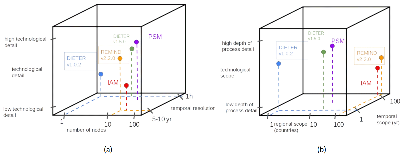
Figure A1Comparison of the (a) resolution and (b) scope for REMIND and a typical IAM as well as two versions of DIETER (v1.0.2 is used in this study) and a typical PSM.
Table A1Comparison between the coupled models REMIND and DIETER.
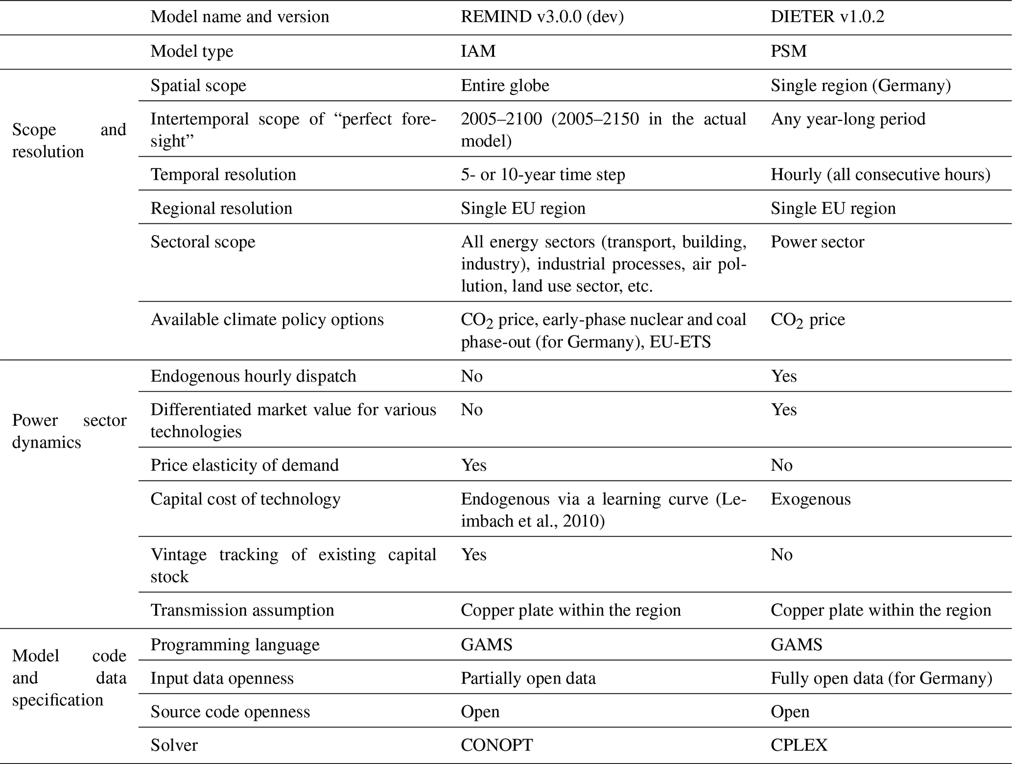
While REMIND and DIETER can both model a European-wide system with spatial subdivision (see Fig. B1 for the REMIND regional division), the soft-coupling is currently only applied to Germany, in line with the proof-of-concept nature of this study. The coupling is from 2020 to 2150 for every defined REMIND period. All common and available REMIND-generating technologies are enabled for the coupling, as shown in Fig. B2. The information for the species of technologies in REMIND is upscaled and coupled to DIETER, whereas information from DIETER is then downscaled during the feedback loop that completes the coupled iteration.
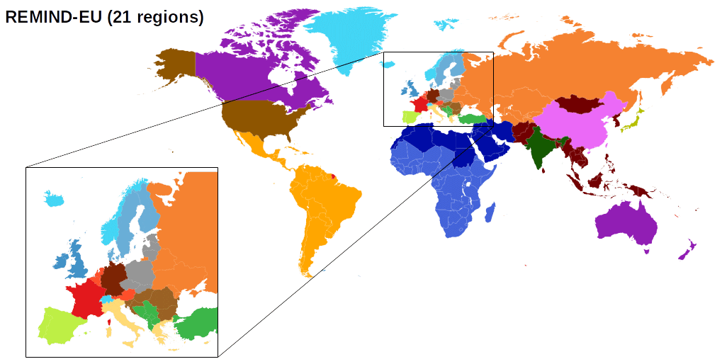
Figure B1REMIND regional resolution used in this study (21 global regions, including detailed differentiations of EU regions). The spatial resolution of REMIND is flexible and depends on the resolution of the input data. Regional mapping is from the REMIND–EU model (Rodrigues et al., 2022).
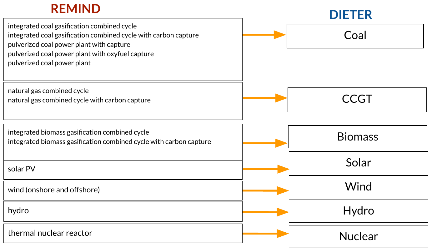
Single-region interannual intertemporal welfare is an aggregated utility, which in turn is a logarithm function of consumption. In REMIND, the total welfare of a region is maximized and is equal to
where regional consumption is χy,reg at model time y and the weight of the consumption is determined by the pure rate of time preference ϱreg and population Vy,reg. The consumption χy,reg at time y is in turn equal to the difference between regional income (gross domestic product – GDP) minus export (which is not available for consumption) and savings (i.e., investments), subtracted by the cost of the energy system (including the power sector) and other costs in the economy. For simplicity we do not discuss several other expenditures, such as capital investment for energy services, other energy-related expenditures such as R&D and innovation, taxes, cost of pollution and land use change.
In Sect. 3.2.1, we sketch the derivation procedure and offer a short summary of the analytical results. Here we describe the derivation procedure of the coupled convergence framework in detail.
Using the Lagrangian multiplier method, based on the objective functions (Eqs. 1–2) and constraints (c1–c6) in Sect. 3.1, we can construct the KKT Lagrangians (Karush, 1939; Kuhn and Tucker, 1951; Gan et al., 2013). REMIND:
DIETER:
Comparing Lagrangians ℒ and , there are notable similarities between the terms. However, first, we can reduce the complexity by noticing that there are terms containing capacity shadow prices that are either trivial or already harmonized: resource constraint shadow prices ω are already identical for both models by design (constraint c2 in Sect. 3.1). Positive generation constraint shadow price ξ is 0 due to KKT conditions for both models (constraint c3). These constraint terms can be safely excluded from the subsequent mapping. We then note the important fact that the REMIND Lagrangian is a sum over multiple years, whereas the DIETER Lagrangian is for each year. To make a direct comparison and therefore mapping possible, we assume that the brown-field and near-term constraints are not binding. After this simplifying assumption, we realize that REMIND becomes linearly independent in terms of the temporal slices because by now the only yet-to-be-harmonized constraints left in the standalone models are (c1) and (c4), which are both constraints for each year and do not result in temporal correlations. Note that this simplifying assumption is assumed to be valid only for the derivation in this section. Later, in actual simulations, we see that these bounds generate shadow prices which are not necessarily small, impacting the degree of convergence, especially in earlier years. These constraints are also temporally localized in early periods, exerting little impact on later, more “green-field” years. In fact, when including the brown-field constraint in DIETER (c8), the model convergence is improved (Sect. 6.1).
After the aforementioned simplifications, we can construct a single-year REMIND Lagrangian ℒy,
and map it to the single-year DIETER Lagrangian :
These are the same as Eqs. (3)–(4).
Comparing ℒy and , we can map them by matching the following four terms in the Lagrangians individually:
- A.
annual total power sector costs: and ;
- B.
annual revenue of usable (post-curtailment) generation for each generator s: and ;
- C.
annual payment made by the consumers: λydy and ; and
- D.
maximum generation from the capacity constraint term for each generator s: and (here we write the two terms for VRE and dispatchable into one term for DIETER for simplicity: i.e., and for dispatchables).
The following conditions (h1–h7) can be derived from the harmonization of terms (A)–(D). Each term is harmonized by matching the values in front of decision variables at the aggregated levels, i.e., capacities and annual generations.
Term (A) can be mapped if
- h1.
annual fixed costs are harmonized for each generator species s: ; and
- h2.
annual variable costs are harmonized for each generator species s: .
Term (B) can be mapped if,
- h3.
for each generator species s, the annual average revenue per unit generation, i.e., the market value, is harmonized by exogenously manipulating the market value in REMIND to be the same as the last-iteration annual average market value in DIETER. We achieve this by adding a correction term, thereby modifying the REMIND original objective function Z to Z′:
where is the markup for technology s in DIETER in the last iteration i−1, and i is the index of the iteration of the iterative soft-coupling. Z′ is the modified REMIND objective function in the coupled version.
The detailed derivation is as follows.
Lagrangian term (B) for the models has the physical meaning of the total annual revenue of usable (post-curtailment) generation. (Annual revenue is equal to the product of usable generation and the annual market value.) We denote total annual revenue from technology s as Θy,s for REMIND and for DIETER. Then, for REMIND, the revenue (term B) is
and for DIETER it is
To harmonize terms Θy,s and , our goal is to create a one-to-one mapping of the values in front of the decision variable's annually aggregated post-curtailment generation of technology s, which is for REMIND and for DIETER. The latter is namely a direct sum of the hourly generations. However, we notice for DIETER revenue that is a weighted sum of the hourly generation, and the direct sum cannot be separated in a straightforward way. So, first we have to rewrite (Eq. D6) by first dividing and then multiplying by the aggregated annual generation:
We notice that the multiplicative term in front of the DIETER annually aggregated generation is , which is nothing other than the market value of generation technology s (see also Eq. F24).
We now take a look at revenue Θy,s on the REMIND side, which is equal to (Eq. D5). To map (D5) to the DIETER revenue term (Eq. D7) in terms of the aggregated decision variables and , we essentially would like the multiplicative term in front of the generation variable in Θy,s, which is λy, to also be like in DIETER. This means that the DIETER-corrected revenue in REMIND should be
To harmonize Θy,s and , we can simply add a linear correction term to compensate for the difference between them. Noticing in Eq. (D5) that the multiplicative term in front of the REMIND generation variable is λy, which can be interpreted as the REMIND market value, we realize essentially for a linear correction term that we should add the market value difference ΔMVy,s between the two models,
to the multiplicative term λy in Θy,s, so λy is canceled. Note that, in Eq. (D9), as discussed before, the DIETER market value is dependent on technology index s, whereas the REMIND one is not.
After adding the linear correction term, the modified revenue in REMIND after harmonization is
Plugging in Eq. (D9),
which is as desired in Eq. (D8).
In practice, in the case of the annual shadow price λy in REMIND, we find that the coupling is more stable numerically if we use the annual average electricity price of DIETER instead of the last-iteration electricity price of REMIND λy in Eq. (D9). The equivalence between the two prices is expressed later in (h5). We can use this substitution, since we show later that (h5) can be derived from market value harmonization (h3) and demand harmonization (h4). With this substitution, the correction term, which we call , is in fact
where is the annual average electricity price in DIETER. We calculate Eq. (D12) using the last-iteration DIETER solutions. Note that, compared to the earlier Eq. (D9), we have simply replaced the second-term REMIND annual price with the DIETER annual price.
It is not hard to recognize as the “markup” for technology s in DIETER, where markup as defined before is the difference between the market value of a technology and the load-weighted annual average electricity price (see the introduction of Sect. 3.1).
Now we have concluded the derivation for the markup term in (h3).
Although the multiplicative terms in front of the decision variables in the two models can be harmonized via the correction term (D12), we notice that it contains endogenous values, i.e., hourly generation and hourly shadow price in DIETER. Since any endogenous value can only be known ex post, this means that the Lagrangian mapping relies on endogenous values from the last iteration, i.e.,
Now, using the markup term , we define the linear correction term for the revenue in REMIND Θy,s as
The physical meaning of ΔΘy,s is the revenue difference in the two models for technology s, given that the post-curtailment generations are expressed in terms of REMIND variables.
The coupled REMIND has a modified objective function Z′ based on a linear correction. The correction term ΔΘy,s needs to be summed over s and y and subtracted – due to the negative sign in front of term (B) – from the REMIND objective function Z, since the objective term as a part of the Lagrangian can be directly manipulated:
where we call the total system revenue differences M; again, these are revenues where the post-curtailment generations are expressed in terms of REMIND variables (and not DIETER variables).
Now we have concluded the derivation for the convergence condition (h3).
Depending on the starting point of the REMIND power system, and due to the internal iterative changes in REMIND results due to the adjustments in trade between regions in the Nash algorithm, coupled convergence usually can only be achieved over multiple iterations. Therefore the derived markup equation (Eq. D12) in general can only be expected to reflect the actual market value differences approximately in the two models. This is the reason why, in the iterative algorithm after the first iteration, we add to the objective function Z, as the quantities and prices gradually converge between the two models. As convergence is approached, the total revenue difference between iterations should go to zero. This is confirmed by the numerical experiments (not shown).
Term (C) can be mapped if
- h4.
annual power demands in the two models are harmonized: ; and
- h5.
annual average prices of electricity are mapped to each other: (dividing term C by h4). Because electricity price is by definition equal to the total annual system revenue divided by the total annual demand, (h5) can be shown to hold true given that technology-specific revenues are harmonized in (h3) and demands are harmonized in (h4). (If technology-specific revenues are harmonized in (h3), then the system revenues which are technology-specific revenues summed over technologies are also harmonized.) Condition (h5) can therefore be seen as a derived condition from (h3) and (h4).
Term (D) can be mapped if
- h6.
annual average capacity factors are harmonized, i.e., ϕy,s in REMIND is set equal to the endogenous last-iteration DIETER result for each generation type s:
where is the hourly capacity factor in DIETER. Without explicit manipulation of the shadow prices μy,s and , we show that the following claim is true: through the above capacity factor harmonization, the terms containing endogenous shadow prices will be automatically mapped. Showing this requires careful mathematical argument, which we make in detail in the case of dispatchables, and later we argue that the case is similar for renewables.
For dispatchable generators the argument is as follows. (For simplicity, we use the generic index s.)
We first rewrite REMIND term (D) by plugging in the harmonization condition :
It should be mapped to the term in DIETER.
Splitting the two terms, these four terms need to be harmonized for all y and s.
To show that the mapping Eqs. (D13)–(D14) are automatically satisfied given (h6), we first consider two simplified power sector toy problems, Q1 and Q2, with only dispatchable technologies. Both problems have identical objective functions , and the fixed and variable cost parameters and are identical. Both problems have identical hourly balance equation constraints but with two different kinds of maximum generation constraints: Q1 has an inequality constraint for each hour, and Q2 has an aggregated annual equality constraint.
Q1: minimum Z, such that ,
Q2: minimum Z, such that ,
Then the Lagrangians are the following:
The relevant KKT conditions are as follows.
Stationarity condition for Q1:
Stationarity condition for Q2:
Since the fixed cost is equal for the two models, from Eqs. (D15) to (D16) we can derive the relation between the two shadow prices:
Note that, for the toy models, the identical balance equation constraints do not contain capacity P, which is why the balance equation constraints do not influence the stationary conditions for P (Eqs. D15–D16).
We now show that Eq. (D14) is automatically mapped given capacity factor harmonization (h6). We first write the equality condition for the REMIND–DIETER case, analogous to the toy model result (Eq. D17):
Note that we can apply the toy model case to the REMIND–DIETER coupling case in a rather straightforward way because, in the case of REMIND–DIETER, the objective function terms have already been harmonized by (h1)–(h2) and the balance equation constraint terms do not contain P, so they have no bearing on the generation-capacity constraint term, just like in the case of the toy models.
Plugging (h6) into Eq. (D18), we have derived the equality for the parameter mapping required in Eq. (D14), i.e.,
To show Eq. (D13), we first use the hourly capacity factor from DIETER,
as well as the primal feasibility condition from REMIND (Eq. F9), to rewrite both sides of the mapping in Eq. (D13) in capacity terms. For REMIND, plugging in Eq. (F9),
and for DIETER, plugging in Eq. (D19),
Take the complementary slackness condition of DIETER (Eq. F16) and insert Eq. (D19) into the left-hand side. We obtain
Rearranging, we get
for each hour h.
Plug Eq. (D22) and then Eq. (D18) into the right-hand side of Eq. (D21) to obtain
Compare Eq. (D20) with Eq. (D23). They now have identical parameters in front of the capacity variables Py,s and , as desired. We concluded the proof by exogenously setting the annual capacity factor of REMIND to that of the last-iteration DIETER. We automatically harmonize the generation capacity constraint term of the Lagrangian in the case of dispatchable generators.
- h7.
For VREs, annual curtailment rates are harmonized, , i.e., by exogenously setting the curtailment rate in REMIND and taking the endogenously determined curtailed power from the last-iteration DIETER. This in general also harmonizes terms other than term (D), as it harmonizes the definition for the generation variable in DIETER that is post-curtailment and the REMIND definition for a generation variable that is pre-curtailment.
For VREs the derivation is conceptually similar to the above case for dispatchables in (h6), since we can define a real capacity factor (post-curtailment) similar to the capacity factor for the dispatchable generators above:
Due to the limitations of this paper, we will not present the derivation here. A detailed derivation is available upon request.
Coupled region: Germany
Coupled REMIND time horizon: 2020–2150 (years 2010–2015 are not coupled since they are historical years and mostly have hard-fixed quantities).
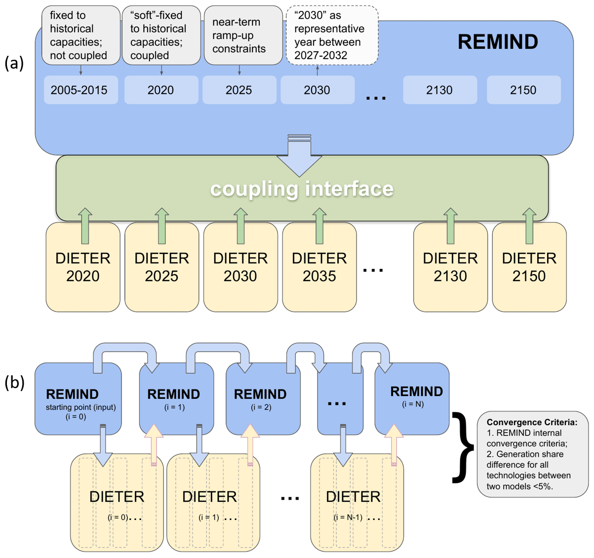
Figure E1A graphic description of the model iterative coupling. (a) Graphic illustration of the bidirectional coupling in the temporal dimension. The temporal slices of REMIND which are mapped to multiple parallel year-long DIETER problems are illustrated here. The convergence conditions are iteratively mapped at the interface. (b) Graphic illustration of the bidirectional coupling in the iteration dimension. Every ith iteration of REMIND takes the (i−1)th iteration of REMIND as a starting point for optimization and the endogenous output of the (i−1)th DIETER as exogenous input parameters. When the convergence conditions are met, i.e., REMIND satisfies its internal convergence condition, and the coupled models differ in their generation share of each technology by at most a certain percentage (e.g., 5 % for the baseline run without storage), the coupled run halts.
Under a simple configuration (no storage, no flexible demand), every REMIND run takes around 3 min and a DIETER run takes a few seconds to solve. Under more detailed configurations (with storage and flexible demand) and climate policies, every REMIND run takes around 4 min and a DIETER run takes a few minutes to solve. The entire REMIND–DIETER coupled run for a single region, Germany, under a simple configuration is around 3–4 h. It is around 6–10 h for the more detailed configurations under climate policies.
In this Appendix, we discuss the equilibrium conditions of the uncoupled models, resulting in a rigorous formulation of the so-called “zero-profit rules” (ZPRs). We first construct the Lagrangians and compute KKT conditions and then derive the ZPRs for the standalone versions of the REMIND-reduced power sector model and the DIETER model.
Using the objective functions and constraints in Sect. 3.1, we can construct Lagrangians for the two standalone models. Using the KKT conditions derived from the Lagrangians, we can show that, if the historical and resource constraints are non-binding, i.e., shadow prices ω, σ and γ are zero, then each generator would have recovered its fixed cost, variable cost and curtailment cost through its total market revenue; i.e., each producer of electricity gets zero profit given that the profits are defined as the difference between revenue and cost. When the capacity constraints exist and are binding, we arrive at a modified version of the original ZPR, which describes the relation between cost, revenue and the capacity shadow prices.
Here we first construct the Lagrangians and derive the KKT conditions from them (Sect. F1) for both models. Then, both models' ZPRs are derived, two for each model, i.e., the technology-specific ZPR and the system ZPR (Sect. F2).
F1 Lagrangians and KKT conditions
The Lagrangians of the uncoupled model have been constructed in Appendix D (Eqs. D1–D2). From the KKT conditions for minimization, we can ascertain the following first-order conditions at stationarity for each model.
REMIND
-
Stationary conditions:
-
Complementary slackness:
-
Primal feasibility:
-
Dual feasibility:
DIETER
-
Stationary conditions:
-
Complementary slackness:
-
Primal feasibility:
-
Dual feasibility:
F2 Derivation of the zero-profit rules
F2.1 REMIND
The derivation of ZPRs is very similar to the one in Brown and Reichenberg (2021). Starting with the total costs for technology s for all years and applying various KKT conditions (after “|”),
Rearranging, we arrive at the ZPR of the multi-year uncoupled REMIND for the technology cost–revenue balance.
Normally when there are no capacity shadow prices or when the capacity constraints are not binding, the cost exactly equals revenue. However, when capacity shadow prices are non-zero, i.e., the constraints (c2) and (c5–c6) are binding, the capacity shadow prices act as a distortion of the equality relation between costs and revenues. As an example, the shadow price ωy,s from limited generation resources (e.g., hydroelectric power in Germany) would be positive, , when the constraint is binding and would appear as a “positive cost” or a “negative revenue” in the modeled power market. We can therefore put it either on the left-hand (cost) or right-hand (revenue) side of the equation. Here we group it together with revenues.
One observes that, from the right-hand side of Eq. (F20), there is no differentiation between the annual market values of variable and dispatchable generations such as gas and solar – they are both equal to the annual electricity price λy.
From Eq. (F20), we can derive a ZPR between the levelized cost of electricity (LCOE), capacity shadow price and market value (MV) for each generator type. Taking Eq. (F20), we separate the pre-curtailment LCOE from the LCOE due to curtailment and then divide it by the total post-curtailment generation for the generator type s to obtain the technology-specific ZPR:
The pre-curtailment LCOE is the cost of one unit of generated electricity, regardless of whether it is curtailed or being used to meet demand, whereas the curtailment LCOE is the cost of one unit of curtailed electricity. Together they add up to the post-curtailment LCOE, i.e., the cost of one unit of usable electricity.
To obtain the ZPR for the whole power system in REMIND, we first sum Eq. (F20) over all generator types s and obtain the ZPR for system cost and revenue. Then, dividing by the total post-curtailment system generation and splitting the LCOE into pre-curtailment and curtailment components, we get
In other words, the LCOE of the system for usable (pre-curtailment) power, which is equal to the sum of the system LCOE for the total power generated and the curtailment cost, can be recovered by the average electricity price of the system minus the system-wide capacity constraint shadow price per energy unit.
The ZPRs of REMIND hold for the aggregate over multiple years.
From Eqs. (F21) and (F22), we learn that when a market equilibrium can be found, i.e., when the optimization problem can be successfully solved, there is an equality relation between the generation cost and market value for each generator type and similarly between the generation cost and price of electricity for the entire system. Capacity shadow prices due to various extra capacity constraints imposed on the models distort the equality relation between costs and prices by a linear term, making the prices either higher or lower than the costs at the market equilibrium.
F2.2 DIETER
Similarly to the uncoupled REMIND, from KKT conditions, at stationarity, we can obtain the cost–revenue ZPR for a single technology s for the standalone DIETER. We take the total costs for technology s for all years and, applying various KKT conditions (after “|”),
Rearranging, we arrive at the ZPR of the single-year uncoupled DIETER for a technology-specific cost–revenue balance:
Dividing Eq. (F23) by the annually aggregated generation of technology s, we obtain the technology-specific ZPR for DIETER:
One observes that, from the term of , compared to the REMIND case (right-hand side of Eq. F21), DIETER has differentiated annual market values of gas and solar generators.
Summing Eq. (F24) over s, dividing both sides by the total annual generation and using the identity for simplification, we obtain the ZPR for the whole power system in DIETER:
Similarly to the case of REMIND, Eqs. (F24)–(F25) show us the equality relations between the cost and value (or price) for each generator type and for the system hold (also for DIETER at its market equilibrium). Compared to REMIND, there are no brown-field or near-term capacity shadow price contributions in DIETER in the standalone versions. The DIETER ZPRs hold for 1 year instead of the aggregate of multiple years like in REMIND. For simplicity, even though it is possible to write the LCOE in pre-curtailment and curtailment terms, for DIETER it is relatively cumbersome to do, and we do not do it here.
In summary, at the REMIND and DIETER power market equilibriums, each generator exactly recovers its cost of one unit of generation through the market value and obtains zero profit in a completely competitive market over its modeling time. In the aggregate, the entire power sector obtains its cost of one unit of generation through the price of electricity that the consumer pays. Both types of relations can be distorted by the existence of capacity shadow prices.
Here, in this Appendix, we gradually build up the derivation for the ZPRs of the coupled REMIND and DIETER, which will be used later to validate numerical results. The derivation consists of three steps.
-
ZPRs for the uncoupled models REMIND and DIETER
-
ZPRs for the coupled models REMIND and DIETER (simplified version only considering convergence conditions h1–h7)
-
ZPRs for the coupled models REMIND and DIETER (full version also considering c7 and c8)
Step (1) is entirely derived in Appendix F.
For step (2), based on the uncoupled ZPRs, we recognize that, from convergence conditions (h1)–(h7), the only condition which impacts the form of the ZPR is (h3) because the markup terms modify the objective function of the (simplified) coupled version of REMIND (Eq. 6). Following a similar procedure to Appendix F, we can derive the technology-specific ZPR for the coupled REMIND (simplified version) as follows:
Compared with the ZPR of the uncoupled version Eq. (F24), the only difference is that we replace the market value in the uncoupled REMIND λy with the DIETER markup-corrected market value . DIETER's ZPR is unchanged at this step.
Step (3) involves two extra capacity constraints, one in each model, the first of which, (c7), is discussed in detail in Appendix H. The implementation of (c7) further modifies Eq. (G1) and results in the ZPRs of the coupled REMIND. The other constraint, (c8), will be the focus of discussion here. It only modifies the ZPRs for the coupled DIETER and not for the coupled REMIND.
Constraint (c8) is a brown-field capacity constraint implemented in DIETER to address the fact that DIETER is a green-field model that is otherwise ignorant of standing capacities in the real world. There are many ways in which we can implement this standing capacity constraint in DIETER. The most straightforward way is to implement the standing capacity at the beginning of each REMIND period, which REMIND sees before it invests additional capacities, as a lower bound on endogenous capacities in DIETER. This helps put DIETER and REMIND on an equal footing before the 5- or 10-year investment period starts, allowing us to compare their investment intentions.
- c8.
Standing capacity constraint in DIETER: i.e., DIETER capacities at time y need to be larger than or equal to the REMIND standing capacities at the beginning of the time period.
where the time step Δy is divided by 2 because the representative year in REMIND is in the middle of the time step. ER is the endogenous early retirement rate in REMIND.
The reason we implement the standing capacity in this way is in part because, as a proof of concept, we want to give DIETER endogenous freedom to invest in all model years, so we use only the pre-investment capacities as “soft” corridors to bound the DIETER capacities from below. If we were to transfer precisely the brown-field and near-term constraints from REMIND to DIETER, this would require a complete list of constraints for each technology and an identical implementation of all of them in DIETER. This may raise the precision of convergence in some years for some technologies, but in practice it can be more complicated to implement than a generic lower bound for all technologies.
To obtain the ZPRs of the coupled DIETER, we simply modify the capacity shadow price term of the uncoupled DIETER ZPRs (Eqs. F24–F25) by the additional capacity shadow price from (c8):
Here, we introduce the two methods we employed to improve the numerical stability of the coupled runs: (1) the dispatchable capacity constraint by peak demand to avoid high markups being exchanged (Sect. H1) and (2) endogenous prefactors for all quantities from the last-iteration DIETER to the current-iteration REMIND (Sect. H2).
H1 Dispatchable capacity constraints by peak demand
H1.1 Description of the capacity constraint and price manipulation in DIETER postprocessing
The scarcity hour price can occur in a PSM run, which is the highest hourly price in a year, and it is usually equal to the annuitized fixed cost of OCGTs (capital investment cost and fixed O&M costs) (Hirth and Ueckerdt, 2013). In our simulations, the scarcity prices are usually above USD 50 per kilowatt hour. If we include the scarcity price in the markups, OCGTs will receive an annual markup usually more than 5 times higher than the annual average electricity price. The high markup results in OCGT plants receiving too high an incentive in the next-iteration REMIND, and the model overshoots (overinvests) in capacities. Over iterations, this causes oscillations in the quantity and prices in the coupled model. For better numerical stability, instead of passing on the full markups from DIETER, we only pass on the portion of the annual markups unrelated to scarcity hour prices and replace the exchange of the part of the markup due to scarcity hours from DIETER to REMIND by implementing an additional capacity constraint in REMIND for coupled runs. The two actions can later be shown to be mathematically equivalent. Generators other than OCGTs which produce at the scarcity hours also get paid in the hour at this high price. However, because they also produce at other hours with lower prices, their average market values are only moderately impacted by the scarcity hour price and do not in general lead to instability issues.
Below, we first introduce the aforementioned capacity constraint implemented on the side of REMIND and then discuss the corresponding manipulation of the markups in DIETER. Lastly, we show their mathematical equivalence and state the modified ZPR of the coupled REMIND due to these actions.
The extra capacity constraint states that the sum of all dispatchable capacities needs to be at least as large as the peak residual demand:
- c7.
where dy,residual is the peak residual demand in REMIND and is semi-endogenous. dy,residual is a function of the peak hourly residual demand in the last iteration of DIETER . The peak hourly residual demand in DIETER is in turn defined as the maximum hourly amount of inflexible demand not met by wind, solar or hydro generations and hence must be met by dispatchable generations (under no storage conditions):
υy,dis is the shadow price of the capacity constraint for dispatchable technology dis.
For the exact implementation of (c7) in the coupled run, see Sects. 3.3.2, point 2. Under storage implementation, in addition to the variable renewable contribution, the hourly storage discharge is also subtracted from the residual demand.
At the same time as implementing this capacity constraint, we remove the surplus scarcity prices in postprocessing of DIETER before passing it on to REMIND. In DIETER, we define the scarcity price as the maximum hourly price in a year,
and the surplus scarcity hour price is the difference between the scarcity price and the second-highest price:
where hscar is the scarcity hour when the scarcity price occurs, corresponding to the peak residual demand hour.
Using this, we manipulate the market value and the annual average electricity price in DIETER ex post, excluding the surplus scarcity hour price:
where is the annual average market value without the surplus scarcity hour price and is the annual average electricity price without the surplus scarcity hour price. Thus, the corresponding modified markup term without the surplus scarcity hour price is
Note that, since the above manipulation is done in a postprocessing step, the LCOE in DIETER is still fully covered by MV, as the KKT conditions and ZPRs still hold by default in an optimized DIETER model.
With the implementation of (c7), the coupled ZPR (Eq. G1) is then further modified to include the new shadow price υy,s and the modified markup (without the surplus scarcity price). (From now on we write υy,dis simply as υy,s.) Then, the technology-specific ZPR of the coupled REMIND is
The system ZPR of the coupled REMIND is
These are the ZPRs of the coupled REMIND for the full version.
H1.2 Equivalence between the surplus scarcity price in DIETER and the capacity shadow price due to the peak residual demand in REMIND
Because of the intuitive relation between the scarcity price and the peak residual demand, i.e., that the scarcity price occurs in the hour with peak hourly residual demand due to the pricing power of the peaker gas turbines in the hour where VREs are most scarce, we can make a quantitative equivalence between the scarcity price contribution to the markup and the capacity constraint shadow price υy. This means that the revenue the plant receives in the scarcity hour in capacity terms (i.e., capacity credit) can be transformed directly to a revenue in energy terms (i.e., a part of the annual market value). At convergence, for any given year y, the negative shadow price, , when translated into annual generation terms via a capacity factor ϕy,s of dispatchable technology s, should be equal to the scarcity hour surplus revenue divided by annual generation by s in DIETER:
In practice, this equivalence is confirmed by numerical results (e.g., the Fig. 8 subplot for OCGTs).
Using this equivalence, we can show as follows that, at convergence, λy should be equal to the DIETER power price without the surplus scarcity price (Eq. H5), and should be equal to the DIETER market value without the scarcity price (Eq. H4).
At convergence, the annual generations have identical solutions in the two models, i.e., . We plug this and the REMIND capacity factor into Eq. (H9) to obtain
Take Eq. (H7) and only consider REMIND annual revenue by multiplying generation . Then, on the right-hand side, take both the revenue and the capacity shadow revenue contribution from υy,s for a single year, which is equal to the total single-year REMIND revenue:
Plug in Eqs. (H10) and (H6):
Plugging in Eq. (H4),
Lastly, plug in the definition for (Eq. H3):
Since the single-year revenue Θy,s in REMIND should be aligned with DIETER due to harmonization condition (h3) and the DIETER revenue is , the last two terms in Eq. (H11) should sum to 0. Therefore, the REMIND electricity price λy should be equal to .
H2 Stabilization techniques using prefactors
In this Appendix, we describe the detailed implementations of prefactors for information exchanged from DIETER to REMIND.
-
Markup prefactor
In order to facilitate convergence in REMIND, we implement an endogenous prefactor for MV in the REMIND markup equation Eq. (5):
The endogenous prefactor is dependent on the difference between the in-iteration endogenous generation share and the last-iteration DIETER generation share:
where is a positive parameter equal to the ratio between market values and the average price, depending on their relationship in the last-iteration DIETER,
and where the generation share difference across the models and consecutive iteration ΔSy,s is
The values of are heuristically determined (see Sect. 6.2).
When the in-iteration REMIND solar generation share increases due to the price signal from the last-iteration DIETER market value, such that the REMIND share is larger than in the last DIETER iteration, the formula Eq. (H13) results in a prefactor smaller than 1, decreasing the in-iteration markup ηy,s(i).
-
Peak demand prefactor
The peak demand in REMIND dresidual,y depends on the last-iteration DIETER peak hourly residual demand . Implementing it in constraint (c7),
for iteration i, we use as a prefactor for stabilization:
by,peak is a heuristic constant dependent on y, and ΔSy,wind is the wind generation share. We use the wind generation share in the current iteration of REMIND for stabilization because, in the peak residual demand hour, there usually is some wind production for the historical year we chose (but no solar). In general, by,peak is 0.5 for earlier years and increases to 1 for later years under a baseline scenario. For climate scenarios, by,peak is around 1.5 for less stringent scenarios, and for more stringent scenarios, it is 0.5 for earlier years and increases to 3 for later years.
-
Capacity factor prefactor
We set the REMIND capacity factor ϕy,dis to be equal to the DIETER annual average capacity factor from the last iteration multiplied by a prefactor:
where the DIETER annual average capacity factor is for each year y. In order to facilitate convergence, a similar prefactor to Eq. (H13) is implemented.
if (i.e., the plant is a “peaker” or “mid-load” type in the last iteration).
if (i.e., the plant is a “base-load” type in the last iteration), where 0.5 is a heuristic factor.
The sign in the prefactor formula is determined based on the observation that, under a system with variable renewable generations, for generator plants that have relatively high running costs and low investment costs, i.e., most economically operated as “peaker” plants or as “mid-load” plants of a lower capacity factor, when their generation share incrementally increases, their capacity factor decreases. Conversely, for generators with relatively low running costs and high investment costs, i.e., most economically operated as “base-load” plants, when their generation share incrementally increases, their capacity factor increases.
-
Curtailment prefactor
The curtailment ratio in REMIND αy,vre is equal to the last-iteration DIETER curtailment ratio multiplied by the prefactor :
where the prefactor is .
-
Capture price prefactor
Similar to the case of markup from the demand side, the markup for any demand-side technology given to REMIND is
where is the annual average electricity price of all demand types sd for period y,
and is an endogenous stabilization prefactor for the flexible-demand markup based on shares of demand by sd in the total demand for each year.
Adjustment cost, an additional linear term in the objective function, acts as an inertia against fast or slow capacity additions or retirement. The implementation of positive adjustment costs mimics the challenges of scaling up the supply chains and training new workers to do installation and construction. Adjustment costs are applied to all model time periods, so it is by nature intertemporal. The objective function for the power sector including the adjustment cost Ξy,s is
where Ξy,s is a quadratic function of the difference between capacity additions of subsequent time periods y−Δy and y:
where ΔPy,s is as before the capacity addition during time period y of technology s, βy,s is an offset parameter to offset additions in initial time periods, ks is a regional technological coefficient, and cy,s is the capital expenditure cost per capacity unit as before. Because the adjustment cost is a quadratic function of the endogenous variable Py,s, it turns the power sector cost minimization in REMIND into a nonlinear problem.
Similar to the case without adjustment costs in Sect. 3.2.3, the first stationary condition becomes
simplifying
where is the endogenous adjustment factor of investment and is a function of capacity.
The new ZPR including the adjustment cost in terms of cost and revenue for technology s can be derived as
The adjustment cost can act as a disincentive or an incentive for capacity additions. If the capacity addition in the current period is higher than in the last period , i.e., a ramp-up case of capacity addition, the adjustment cost is positive and acts as a disincentive, and so the ramp-up speed is slower. When added capacities decrease with time, i.e., a ramp-down case of capacity addition, the adjustment cost is negative and acts as an incentive; as a result, the ramp-down speed is slower.
In the coupled run we see only a moderate adjustment cost which drops down quickly as a function of time (see, e.g., Fig. 6).
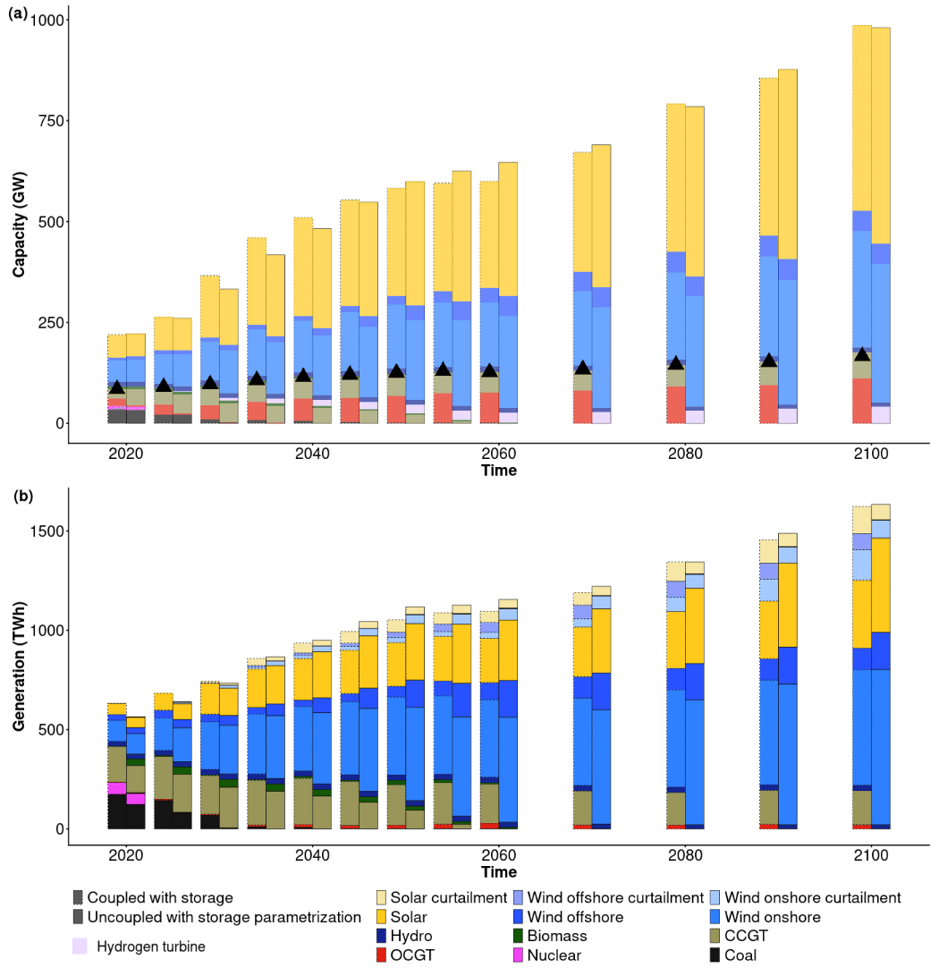
Figure J1Under the 2 ∘C global scenario (no German net-zero goal), we compare (a) the capacity mix and (b) the generation mix of Germany for the DIETER-coupled version of REMIND with endogenous storage (dashed bar) and for the uncoupled version of REMIND with parameterized storage (solid bar). In panel (a), triangle dots indicate the peak residual demand of the year as determined in DIETER.
The units used in the two models are usually different. Here we uniformly use megawatt hour for energy units and megawatt for capacity units. In the main text, overline is used to denote DIETER parameters and variables. An apostrophe is used to indicate a modified version of the variable. An asterisk is used to indicate the values of variables at the optimum of objective functions.
Table K1Complete list of mathematical symbols. For simplicity, in general, we only list the symbols, not their indices or in which model they are used.
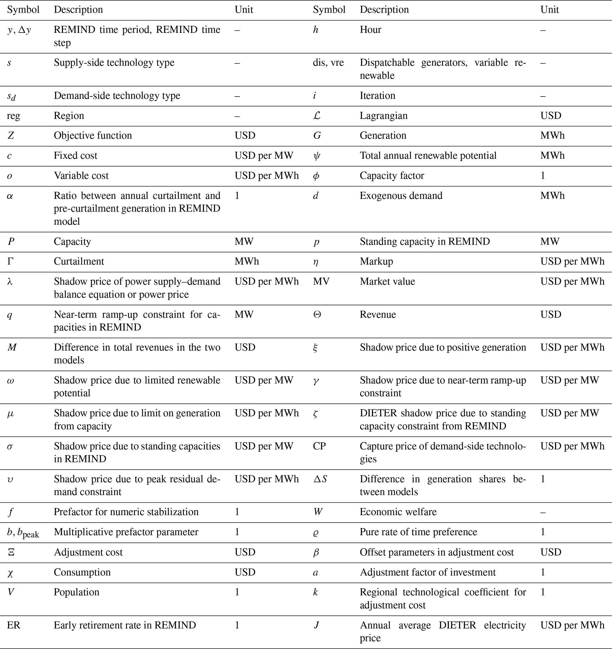
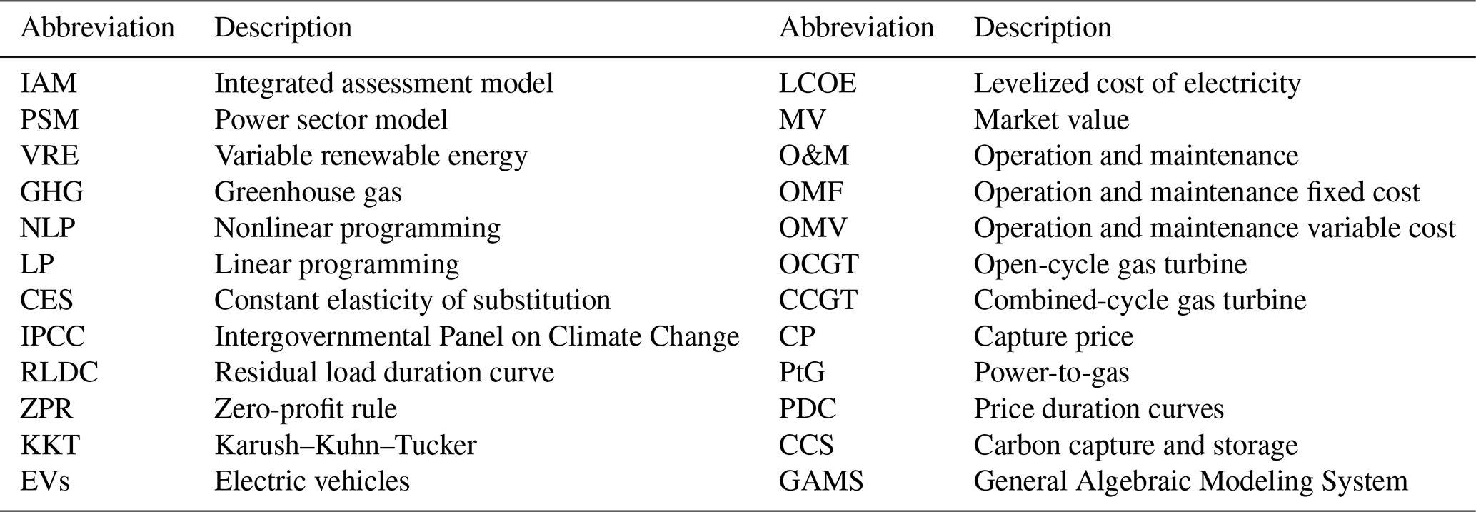
The coupled and uncoupled REMIND codes are implemented in GAMS, and the code and data management is done using R. The coupled and uncoupled DIETER models are entirely implemented in GAMS. The default uncoupled REMIND v3.0.0 code is available from the GitHub website at https://github.com/remindmodel/remind (Gong, 2022a) and is archived at Zenodo under the GNU Affero General Public License, version 3 (AGPLv3) (https://doi.org/10.5281/zenodo.6794920, Luderer et al., 2022b). The technical model documentation is available at https://rse.pik-potsdam.de/doc/remind/3.0.0/ (last access: 1 September 2022, Luderer et al., 2020). The coupled version of REMIND is available at https://github.com/cchrisgong/remind-coupling-dieter/tree/couple (last access: 2 September 2022); the coupled DIETER is available at https://github.com/cchrisgong/dieter-coupling-remind (Gong, 2022b). The two sets of coupling codes are archived at Zenodo under the Creative Commons Attribution 4.0 International License (https://doi.org/10.5281/zenodo.705324, Luderer et al., 2022c). The GAMS code, results and scripts to produce the figures shown in this paper are archived at Zenodo (https://doi.org/10.5281/zenodo.7072625, Gong, 2022c).
The supplement related to this article is available online at: https://doi.org/10.5194/gmd-16-4977-2023-supplement.
Methodology development was done by CG, FU and RP. CG designed and carried out the numerical implementation and performed the theoretical analysis of the methodology. The methodology was first conceptualized by GL. Supervision and funding acquisition were carried out by FU and GL. OA participated in the development of model postprocessing and the overall structuring of the manuscript. MK and WPS performed theoretical and conceptual validation of the manuscript. CG prepared the manuscript with contributions from all the co-authors.
At least one of the (co-)authors is a member of the editorial board of Geoscientific Model Development. The peer-review process was guided by an independent editor, and the authors also have no other competing interests to declare.
Publisher's note: Copernicus Publications remains neutral with regard to jurisdictional claims in published maps and institutional affiliations.
The authors thank Tom Brown at the Technical University of Berlin as well as Marian Leimbach, Renato Rodrigues, Nico Bauer, and Christof Schoetz at the Potsdam Institute for Climate Impact Research for discussion.
This research has been supported by the Bundesministerium für Bildung und Forschung (grant nos. 03SFK5N0, 03SFK5A and 01LP1928A) and the Deutsche Bundesstiftung Umwelt (PhD scholarship).
The article processing charges for this open-access publication were covered by the Potsdam Institute for Climate Impact Research (PIK).
This paper was edited by Sam Rabin and reviewed by two anonymous referees.
Alimou, Y., Maïzi, N., Bourmaud, J.-Y., and Li, M.: Assessing the security of electricity supply through multi-scale modeling: The TIMES-ANTARES linking approach, Appl. Energ., 279, 115717, https://doi.org/10.1016/j.apenergy.2020.115717, 2020.
Aryanpur, V., O'Gallachoir, B., Dai, H., Chen, W., and Glynn, J.: A review of spatial resolution and regionalisation in national-scale energy systems optimisation models, Energy Strateg. Rev., 37, 100702, https://doi.org/10.1016/j.esr.2021.100702, 2021.
Azevedo, I., Bataille, C., Bistline, J., Clarke, L., and Davis, S.: Net-zero emissions energy systems: What we know and do not know, Energy Clim. Change, 2, 100049, https://doi.org/10.1016/j.egycc.2021.100049, 2021.
Bauer, N., Calvin, K., Emmerling, J., Fricko, O., Fujimori, S., Hilaire, J., Eom, J., Krey, V., Kriegler, E., Mouratiadou, I., Sytze de Boer, H., van den Berg, M., Carrara, S., Daioglou, V., Drouet, L., Edmonds, J. E., Gernaat, D., Havlik, P., Johnson, N., Klein, D., Kyle, P., Marangoni, G., Masui, T., Pietzcker, R. C., Strubegger, M., Wise, M., Riahi, K., and van Vuuren, D. P.: Shared Socio-Economic Pathways of the Energy Sector – Quantifying the Narratives, Global Environ. Chang., 42, 316–330, https://doi.org/10.1016/j.gloenvcha.2016.07.006, 2017.
Baumstark, L., Bauer, N., Benke, F., Bertram, C., Bi, S., Gong, C. C., Dietrich, J. P., Dirnaichner, A., Giannousakis, A., Hilaire, J., Klein, D., Koch, J., Leimbach, M., Levesque, A., Madeddu, S., Malik, A., Merfort, A., Merfort, L., Odenweller, A., Pehl, M., Pietzcker, R. C., Piontek, F., Rauner, S., Rodrigues, R., Rottoli, M., Schreyer, F., Schultes, A., Soergel, B., Soergel, D., Strefler, J., Ueckerdt, F., Kriegler, E., and Luderer, G.: REMIND2.1: transformation and innovation dynamics of the energy-economic system within climate and sustainability limits, Geosci. Model Dev., 14, 6571–6603, https://doi.org/10.5194/gmd-14-6571-2021, 2021.
Bhaskar, A., Assadi, M., and Nikpey Somehsaraei, H.: Decarbonization of the Iron and Steel Industry with Direct Reduction of Iron Ore with Green Hydrogen, Energies, 13, 758, https://doi.org/10.3390/en13030758, 2020.
Bistline, J. E. T.: The importance of temporal resolution in modeling deep decarbonization of the electric power sector, Environ. Res. Lett., 16, 084005, https://doi.org/10.1088/1748-9326/ac10df, 2021.
Blanford, G. J. and Weissbart, C.: A Framework for Modeling the Dynamics of Power Markets – The EU-REGEN Model, ifo Working Paper Series, ifo Institute – Leibniz Institute for Economic Research at the University of Munich, https://www.ifo.de/en/publications/2019/working-paper/framework-modeling-dynamics-power-markets-eu-regen-model (last access: 22 January 2022), 2019.
Böttger, D. and Härtel, P.: On wholesale electricity prices and market values in a carbon-neutral energy system, Energy Econ., 106, 105709, https://doi.org/10.1016/j.eneco.2021.105709, 2022.
Brinkerink, M.: Assessing 1.5–2 ∘C scenarios of integrated assessment models from a power system perspective – Linkage with a detailed hourly global electricity model, Monograph, IIASA, Laxenburg, Austria, https://pure.iiasa.ac.at/id/eprint/16957/ (last access: 22 January 2022), 2020.
Brinkerink, M., Zakeri, B., Huppmann, D., Glynn, J., Ó Gallachóir, B., and Deane, P.: Assessing global climate change mitigation scenarios from a power system perspective using a novel multi-model framework, Environ. Modell. Softw., 150, 105336, https://doi.org/10.1016/j.envsoft.2022.105336, 2022.
Brown, T. and Reichenberg, L.: Decreasing market value of variable renewables can be avoided by policy action, Energy Econ., 100, 105354, https://doi.org/10.1016/j.eneco.2021.105354, 2021.
Brown, T., Hörsch, J., and Schlachtberger, D.: PyPSA: Python for Power System Analysis, J. Open Res. Softw., 6, 4, https://doi.org/10.5334/jors.188, 2018a.
Brown, T., Schlachtberger, D., Kies, A., Schramm, S., and Greiner, M.: Synergies of sector coupling and transmission reinforcement in a cost-optimised, highly renewable European energy system, Energy, 160, 720–739, https://doi.org/10.1016/j.energy.2018.06.222, 2018b.
Brunner, C., Deac, G., Braun, S., and Zöphel, C.: The future need for flexibility and the impact of fluctuating renewable power generation, Renew. Energy, 149, 1314–1324, https://doi.org/10.1016/j.renene.2019.10.128, 2020.
Butnar, I., Li, P.-H., Strachan, N., Portugal Pereira, J., Gambhir, A., and Smith, P.: A deep dive into the modelling assumptions for biomass with carbon capture and storage (BECCS): A transparency exercise, Environ. Res. Lett., 15, 084008, https://doi.org/10.1088/1748-9326/ab5c3e, 2019.
Calvin, K., Bond-Lamberty, B., Clarke, L., Edmonds, J., Eom, J., Hartin, C., Kim, S., Kyle, P., Link, R., Moss, R., McJeon, H., Patel, P., Smith, S., Waldhoff, S., and Wise, M.: The SSP4: A world of deepening inequality, Global Environ. Chang., 42, 284–296, https://doi.org/10.1016/j.gloenvcha.2016.06.010, 2017.
Chang, M., Thellufsen, J. Z., Zakeri, B., Pickering, B., Pfenninger, S., Lund, H., and Østergaard, P. A.: Trends in tools and approaches for modelling the energy transition, Appl. Energ., 290, 116731, https://doi.org/10.1016/j.apenergy.2021.116731, 2021.
Cherp, A., Vinichenko, V., Tosun, J., Gordon, J. A., and Jewell, J.: National growth dynamics of wind and solar power compared to the growth required for global climate targets, Nat. Energy, 6, 742–754, https://doi.org/10.1038/s41560-021-00863-0, 2021.
Clarke, L., Wei, Y.-M., De La Vega Navarro, A., Garg, A., Hahmann, A. N., Khennas, S., Azevedo, I. M. L., Löschel, A., Singh, A. K., Steg, L., Strbac, G., and Wada, K.: Energy Systems, in: IPCC, 2022: Climate Change 2022: Mitigation of Climate Change, Contribution of Working Group III to the Sixth Assessment Report of the Intergovernmental Panel on Climate Change, 219, https://doi.org/10.1017/9781009157926.008, 2022.
Conejo, A. J., Castillo, E., Mínguez R., and García-Bertrand, R.: Decomposition techniques in mathematical programming, Springer-Verlag Berlin Heidelberg, https://doi.org/10.1007/3-540-27686-6, 2006.
Creutzig, F., Agoston, P., Goldschmidt, J. C., Luderer, G., Nemet, G., and Pietzcker, R. C.: The underestimated potential of solar energy to mitigate climate change, Nat. Energy, 2, 17140, https://doi.org/10.1038/nenergy.2017.140, 2017.
Deane, J. P., Chiodi, A., Gargiulo, M., and Ó Gallachóir, B. P.: Soft-linking of a power systems model to an energy systems model, Energy, 42, 303–312, https://doi.org/10.1016/j.energy.2012.03.052, 2012,
E3MLab, PRIMES Model Version 2018 – detailed model description, http://www.e3mlab.ntua.gr/e3mlab/PRIMES (last access: 4 May 2023), 2018.
Ellenbeck, S. and Lilliestam, J.: How modelers construct energy costs: Discursive elements in Energy System and Integrated Assessment Models, Energy Res. Soc. Sci., 47, 69–770, https://doi.org/10.1016/j.erss.2018.08.021, 2019.
Figueiredo, N. C. and da Silva, P. P.: The price of wind power generation in Iberia and the merit-order effect, International Journal of Sustainable Energy Planning and Management, 15, 21–30, https://doi.org/10.5278/ijsepm.2018.15.4, 2018.
Frysztacki, M. M., Hörsch, J., Hagenmeyer, V., and Brown, T.: The strong effect of network resolution on electricity system models with high shares of wind and solar, Appl. Energ., 291, 116726, https://doi.org/10.1016/j.apenergy.2021.116726, 2021.
Frysztacki, M. M., Recht, G., and Brown, T., A comparison of clustering methods for the spatial reduction of renewable electricity optimisation models of Europe, Energy Inform., 5, 4, https://doi.org/10.1186/s42162-022-00187-7, 2022.
Fuso Nerini, F., Keppo, I., and Strachan, N.: Myopic decision making in energy system decarbonisation pathways. A UK case study, Energy Strateg. Rev., 17, 19–26, https://doi.org/10.1016/j.esr.2017.06.001, 2017.
Gaete-Morales, C., Kittel, M., Roth, A., and Schill, W.-P.: DIETERpy: A Python framework for the Dispatch and Investment Evaluation Tool with Endogenous Renewables, SoftwareX, 15, 100784, https://doi.org/10.1016/j.softx.2021.100784, 2021.
Gan, D., Feng, D., and Xie, J.: Electricity Markets and Power System Economics, CRC Press, Boca Raton, 220 pp., https://doi.org/10.1201/b15550, 2013.
Geels, F., Berkhout, F. and van Vuuren, D.: Bridging analytical approaches for low-carbon transitions, Nat. Clim. Change, 6, 576–583, https://doi.org/10.1038/nclimate2980, 2016.
Giarola, S., Mittal, S., Vielle, M., Perdana, S., Campagnolo, L., Delpiazzo, E., Bui, H., Kraavi, A. A., Kolpakov, A., Sognnaes, I., Peters, G., Hawkes, A., Köberle, A. C., Grant, N., Gambhir, A., Nikas, A., Doukas, H., Moreno, J., and van de Ven, D.-J.: Challenges in the harmonisation of global integrated assessment models: A comprehensive methodology to reduce model response heterogeneity, Sci. Total Environ., 783, 146861, https://doi.org/10.1016/j.scitotenv.2021.146861, 2021.
Gils, H. C., Gardian, H., Kittel, M., Schill, W.-P., Zerrahn, A., Murmann, A., Launer, J., Fehler, A., Gaumnitz, F., van Ouwerkerk, J., Bußar, C., Mikurda, J., Torralba-Díaz, L., Janßen, T., and Krüger, C.: Modeling flexibility in energy systems – comparison of power sector models based on simplified test cases, Renew. Sust. Energ. Rev., 158, 111995, https://doi.org/10.1016/j.rser.2021.111995, 2022a.
Gils, H. C., Gardian, H., Kittel, M., Schill, W.-P., Murmann, A., Launer, J., Gaumnitz, F., van Ouwerkerk, J., Mikurda, J., and Torralba-Díaz, L.: Model-related outcome differences in power system models with sector coupling – Quantification and drivers, Renew. Sust. Energ. Rev., 159, 112177, https://doi.org/10.1016/j.rser.2022.112177, 2022b.
Gong, C. C.: remind-coupling-dieter[code], REMIND – REgional Model of INvestments and Development, GitHub [code], https://github.com/cchrisgong/remind-coupling-dieter/tree/couple (last access: 1 September 2022), 2022a.
Gong, C. C.: dieter-coupling-remind[code], GAMS, REMIND – REgional Model of INvestments and Development, GitHub [code], https://github.com/cchrisgong/dieter-coupling-remind (last access: 1 September 2022), 2022b.
Gong, C. C.: REMIND-DIETER – code, reportings, scripts, Zenodo [code], https://doi.org/10.5281/zenodo.7072625, 2022c.
Griffiths, S., Sovacool, B. K., Kim, J., Bazilian, M., and Uratani, J. M.: Industrial decarbonization via hydrogen: A critical and systematic review of developments, socio-technical systems and policy options, Energy Res. Soc. Sci., 80, 102208, https://doi.org/10.1016/j.erss.2021.102208, 2021.
Guivarch, C., Kriegler, E., Portugal-Pereira, J., and Bosetti, V.: IPCC, 2022: Annex III: Scenarios and modelling methods, in: IPCC, 2022: Climate Change 2022: Mitigation of Climate Change. Contribution of Working Group III to the Sixth Assessment Report of the Intergovernmental Panel on Climate Change, Cambridge University Press, Cambridge, United Kingdom and New York, NY, USA, https://doi.org/10.1017/9781009157926.022, 2022.
Günther, C., Schill, W.-P., and Zerrahn, A.: Prosumage of solar electricity: Tariff design, capacity investments, and power sector effects, Energ. Policy, 152, 112168, https://doi.org/10.1016/j.enpol.2021.112168, 2021.
Guo, F., van Ruijven, B. J., Zakeri, B., Zhang, S., Chen, X., Liu, C., Yang, F., Krey, V., Riahi, K., Huang, H., and Zhou, Y.: Implications of intercontinental renewable electricity trade for energy systems and emissions, Nat. Energy, 7, 1144–1156, https://doi.org/10.1038/s41560-022-01136-0, 2022.
Haydt, G., Leal, V., Pina, A., and Silva, C. A.: The relevance of the energy resource dynamics in the mid/long-term energy planning models, Renew. Energy, 36, 3068–3074, 2011.
Hildmann, M., Ulbig, A., and Andersson, G.: Empirical Analysis of the Merit-Order Effect and the Missing Money Problem in Power Markets With High RES Shares, IEEE T. Power Syst., 30, 1560–1570, https://doi.org/10.1109/TPWRS.2015.2412376, 2015.
Hirth, L.: The market value of variable renewables: The effect of solar wind power variability on their relative price, Energy Econ., 38, 218–236, https://doi.org/10.1016/j.eneco.2013.02.004, 2013.
Hirth, L.: What caused the drop in European electricity prices? A factor decomposition analysis, Energy J., 39, 1, https://doi.org/10.5547/01956574.39.1.lhir, 2018.
Hirth, L. and Ueckerdt, F.: Redistribution effects of energy and climate policy: The electricity market, Energ. Policy, 62, 934–947, https://doi.org/10.1016/j.enpol.2013.07.055, 2013.
Huppmann, D., Gidden, M., Fricko, O., Kolp, P., Orthofer, C., Pimmer, M., Kushin, N., Vinca, A., Mastrucci, A., Riahi, K., and Krey, V.: The MESSAGEix Integrated Assessment Model and the ix modeling platform (ixmp): An open framework for integrated and cross-cutting analysis of energy, climate, the environment, and sustainable development, Environ. Modell. Softw., 112, 143–156, https://doi.org/10.1016/j.envsoft.2018.11.012, 2019.
ICCSD Tsinghua University: Power Sector, in: China's Long-Term Low-Carbon Development Strategies and Pathways: Comprehensive Report, edited by: Institute of Climate Change and Sustainable Development of Tsinghua University, Springer, Singapore, 109–130, https://doi.org/10.1007/978-981-16-2524-4_4, 2022.
IEA: World Energy Outlook 2021, https://www.iea.org/reports/world-energy-outlook-2021 (last access: 21 January 2022), 2021.
IPCC: Climate change 2014: mitigation of climate change: Working Group III contribution to the Fifth assessment report of the Intergovernmental Panel on Climate Change, edited by: Edenhofer, O., Pichs-Madruga, R., Sokona, Y., Farahani, E., Kadner, S., Seyboth, K., Alder, A., Baum, I., Brunner, S., Eikemeier, P., Kriemann, B., Salolainen, J., Schlömer, S., Stechow, C. von, Zwickel, T., and Minx, J. C., Cambridge University Press, Cambridge, United Kingdom and New York, NY, USA, https://doi.org/10.1017/CBO9781107415416, 2014.
IPCC: Climate Change 2022: Mitigation of Climate Change, Contribution of Working Group III to the Sixth Assessment Report of the Intergovernmental Panel on Climate Change, edited by: Shukla, P. R., Skea, J., Slade, R., Al Khourdajie, A., van Diemen, R., McCollum, D., Pathak, M., Some, S., Vyas, P., Fradera, R., Belkacemi, M., Hasija, A., Lisboa, G., Luz, S., and Malley, J., Cambridge University Press, Cambridge, UK and New York, NY, USA, https://doi.org/10.1017/9781009157926, 2022.
IRENA: Renewable power generation costs in 2019, International Renewable Energy Agency, ISBN 978-92-9260-244-4, 2020.
Kannan, R. and Turton, H.: A Long-Term Electricity Dispatch Model with the TIMES Framework, Environ. Model. Assess., 18, 325–343, https://doi.org/10.1007/s10666-012-9346-y, 2013.
Karush, W.: Minima of functions of several variables with inequalities as side conditions (William Karush), Master's thesis, Department of Mathematics, University of Chicago, 1939.
Keppo, I., Butnar, I., Bauer, N., Caspani, M., Edelenbosch, O., Emmerling, J., Fragkos, P., Guivarch, C., Harmsen, M., Lefèvre, J., Le Gallic, T., Leimbach, M., McDowall, W., Mercure, J.-F., Schaeffer, R., Trutnevyte, E., and Wagner, F.: Exploring the possibility space: taking stock of the diverse capabilities and gaps in integrated assessment models, Environ. Res. Lett., 16, 053006, https://doi.org/10.1088/1748-9326/abe5d8, 2021.
Koch, J. and Leimbach, M.: Update of Ssp GDP Projections: Capturing Recent Changes in National Accounting, PPP Conversion and Covid 19 Impacts, Ecol. Econ., 206, https://doi.org/10.2139/ssrn.4011838, 2023.
Koutstaal, P. R. and va. Hout, M.: Integration costs and market value of variable renewables: A study for the Dutch power market, ECN, Petten, http://resolver.tudelft.nl/uuid:a36bc05a-6a36-428f-9ff6-e33141fcf167 (last access: 22 January 2022), 2017.
Kuhn, H. W. and Tucker, A. W.: Nonlinear Programming, in: Traces and Emergence of Nonlinear Programming, edited by: Giorgi, G. and Kjeldsen, T., Birkhäuser, Basel, https://doi.org/10.1007/978-3-0348-0439-4_11, 1951.
Lazard: Lazard's Levelized Cost of Energy Analysis – Version 15.0, https://www.lazard.com/media/sptlfats/lazards-levelized-cost-of-energy-version-150-vf.pdf (last access: 21 January 2022), 2021.
Levesque, A., Pietzcker, R. C., Baumstark, L., De Stercke, S., Grübler, A., Luderer, G.: How much energy will buildings consume in 2100? A global perspective within a scenario framework, Energy, 148, 514–527, https://doi.org/10.1016/j.energy.2018.01.139, 2018.
Leimbach, M., Bauer, N., Baumstark, L., Luken, M., and Edenhofer, O.: Technological Change and International Trade – Insights from REMIND-R, Energy J., 31, 109–136, https://doi.org/10.5547/ISSN0195-6574-EJ-Vol31-NoSI-5, 2010.
Li, P.-H. and Pye, S.: Assessing the benefits of demand-side flexibility in residential and transport sectors from an integrated energy systems perspective, Appl. Energ., 228, 965–979, https://doi.org/10.1016/j.apenergy.2018.06.153, 2018.
López Prol, J. and Schill, W.-P.: The Economics of Variable Renewable Energy and Electricity Storage, Annu. Rev. Resour. Econ., 13, 443–467, https://doi.org/10.1146/annurev-resource-101620-081246, 2021.
Luderer, G., Pietzcker, R. C., Carrara, S., de Boer, H. S., Fujimori, S., Johnson, N., Mima, S., and Arent, D.: Assessment of wind and solar power in global low-carbon energy scenarios: An introduction, Energy Econ., 64, 542–551, https://doi.org/10.1016/j.eneco.2017.03.027, 2017.
Luderer, G., Vrontisi, Z., Bertram, C., Edelenbosch, O., Pietzcker, R. C., Rogelj, J., De Boer, H. S., Drouet, L., Emmerling, J., Fricko, O., Fujimori, S., Havlik, P., Iyer, G., Keramidas, K., Kitous, A., Pehl, M., Krey, V., Riahi, K., Saveyn, B., Tavoni, M., Van Vuuren, D. P., and Kriegler, E.: Residual fossil CO2 emissions in 1.5–2∘C pathways, Nat. Clim. Change, 8, 626–633, https://doi.org/10.1038/s41558-018-0198-6, 2018.
Luderer, G., Auer, C., Bauer, N., Baumstark, L., Bertram, C., Bi, S., Dirnaichner, A., Giannousakis, A., Hilaire, J., Klein, D., Koch, J., Leimbach, M., Levesque, A., Malik, A., Merfort, L., Pehl, M., Pietzker, R., Piontek, F., Rauner, S., Rodrigues, R., Rottoli, M., Schreyer, F., Sörgel, B., Strefler, J., and Ueckerdt, F.: REMIND v2.1.3 – Model documentation, Zenodo, https://doi.org/10.5281/zenodo.4268254, 2020.
Luderer, G., Madeddu, S., Merfort, L., Ueckerdt, F., Pehl, M., Pietzcker, R., Rottoli, M., Schreyer, F., Bauer, N., Baumstark, L., Bertram, C., Dirnaichner, A., Humpenöder, F., Levesque, A., Popp, A., Rodrigues, R., Strefler, J., and Kriegler, E.: Impact of declining renewable energy costs on electrification in low-emission scenarios, Nat. Energy, 7, 32–42, https://doi.org/10.1038/s41560-021-00937-z, 2022a.
Luderer, G., Bauer, N., Baumstark, L., Bertram, C., Leimbach, M., Pietzcker, R., Strefler, J., Aboumahboub, T., Abrahão, G., Auer, C., Benke, F., Bi, S., Dietrich, J., Dirnaichner, A., Giannousakis, A., Gong, C. C., Haller, M., Hasse, R., Hilaire, J., Hoppe, J., Klein, D., Koch, J., Körner, A., Kowalczyk, K., Kriegler, E., Levesque, A., Lorenz, A., Ludig, S., Lüken, M., Malik, A., Manger, S., Merfort, A., Merfort, L., Moreno-Leiva, S., Mouratiadou, I., Odenweller, A., Pehl, M., Piontek, F., Popin, L., Rauner, S., Richters, O., Rodrigues, R., Roming, N., Rottoli, M., Schmidt, E., Schötz, C., Schreyer, F., Schultes, A., Sörgel, B., Ueckerdt, F., Verpoort, P., and Weigmann, P.: REMIND – REgional Model of INvestments and Development, Zenodo [code], https://doi.org/10.5281/zenodo.6794920, 2022b.
Luderer, G., Bauer, N., Gong, C. C., Odenweller, A., Baumstark, L., Bertram, C., Leimbach, M., Pietzcker, R., Strefler, J., Aboumahboub, T., Abrahão, G., Auer, C., Benke, F., Bi, S., Dietrich, J., Dirnaichner, A., Giannousakis, A., Haller, M., Hasse, R., Hilaire, J., Hoppe, J., Klein, D., Koch, J., Kowalczyk, K., Kriegler, E., Levesque, A., Ludig, S., Malik, A., Merfort, A., Merfort, L., Moreno, S., Mouratiadou, I., Pehl, M., Piontek, F., Popin, L., Rauner, S., Richters, O., Schötz, C., Rodrigues, R., Ueckerdt, F., Zerrahn, A., Schreyer, F., Sörgel, B., Weigmann, P., Schill, W.-P., Verpoort, P., and Rottoli, M.: REMIND – DIETER coupling, Zenodo [code], https://doi.org/10.5281/zenodo.7053246, 2022c.
Ludig, S., Haller, M., Schmid, E., and Bauer, N.: Fluctuating renewables in a long-term climate change mitigation strategy, Energy, 36, 6674–6685, https://doi.org/10.1016/j.energy.2011.08.021, 2011.
Martínez-Gordón, R., Morales-España, G., Sijm, J., and Faaij, A. P. C.: A review of the role of spatial resolution in energy systems modelling: Lessons learned and applicability to the North Sea region, Renew. Sust. Energ. Rev., 141, 110857, https://doi.org/10.1016/j.rser.2021.110857, 2021.
Mills, A. D. and Wiser, R. H.: Strategies to mitigate declines in the economic value of wind and solar at high penetration in California, Appl. Energ., 147, 269–278, https://doi.org/10.1016/j.apenergy.2015.03.014, 2015.
Mowers, M., Mignone, B. K. and Steinberg, D. C.: Quantifying value and representing competitiveness of electricity system technologies in economic models, Appl. Energ., 329, 120132, https://doi.org/10.1016/j.apenergy.2022.120132, 2023.
National long-term strategies: https://ec.europa.eu/info/energy-climate-change-environment/implementation-eu-countries/energy-and-climate-governance-and-reporting/national-long-term-strategies_en, last access: 15 January 2022.
NGFS: NGFS Climate Scenarios for central banks and supervisors, Network for Greening the Financial System, https://www.ngfs.net/en/ngfs-climate-scenarios-central-banks-and-supervisors-september-2022 (last access: 23 August 2023), 2022.
openmod – Open Energy Modelling Initiative: https://openmod-initiative.org/, last access: 21 January 2022.
Padhy, N. P.: Unit commitment-a bibliographical survey, IEEE T. Power Syst., 19, 1196–1205, https://doi.org/10.1109/TPWRS.2003.821611, 2004.
Pahle, M., Tietjen, O., Osorio, S., Egli, F., Steffen, B., Schmidt, T. S. and Edenhofer O.: Safeguarding the energy transition against political backlash to carbon markets, Nat. Energy, 7, 290–296, https://doi.org/10.1038/s41560-022-00984-0, 2022.
Palzer, A. and Henning, H.-M.: A Future German Energy System with a Dominating Contribution from Renewable Energies: A Holistic Model Based on Hourly Simulation, Energy Technol., 2, 13–28, https://doi.org/10.1002/ente.201300083, 2014.
Parra, D., Valverde, L., Pino, F. J., and Patel, M. K.: A review on the role, cost and value of hydrogen energy systems for deep decarbonisation, Renew. Sust. Energ. Rev., 101, 279–294, https://doi.org/10.1016/j.rser.2018.11.010, 2019.
Pietzcker, R. C., Ueckerdt, F., Carrara, S., de Boer, H. S., Després, J., Fujimori, S., Johnson, N., Kitous, A., Scholz, Y., Sullivan, P., and Luderer, G.: System integration of wind and solar power in integrated assessment models: A cross-model evaluation of new approaches, Energy Econ., 64, 583–599, https://doi.org/10.1016/j.eneco.2016.11.018, 2017.
Pina, A., Silva, C., and Ferrão, P.: Modeling hourly electricity dynamics for policy making in long-term scenarios, Energ. Policy, 39, 4692–4702, https://doi.org/10.1016/j.enpol.2011.06.062, 2011.
Prina, M. G., Manzolini, G., Moser, D., Nastasi, B., and Sparber, W.: Classification and challenges of bottom-up energy system models – A review, Renew. Sust. Energ. Rev., 129, 109917, https://doi.org/10.1016/j.rser.2020.109917, 2020.
Prol, J. L. and Schill, W.-P.: The Economics of Variable Renewable Energy and Electricity Storage, Annual Review of Resource Economics, 13, 443–467, https://doi.org/10.1146/annurev-resource-101620-081246, 2021.
Ram, M., Bogdanov, D., Aghahosseini, A., Gulagi, A., Oyewo, S., Child, M., Caldera, U., Sadovskaia, K., Farfan Orozco, F., Noel, L., Fasihi, M., Maybodi, S., and Fell, H.-J.: Global Energy System based on 100 % Renewable Energy: Energy Transition in Europe Across Power, Heat, Transport and Desalination Sectors, Technical report, https://doi.org/10.13140/RG.2.2.10143.00160, 2018.
Ramsebner, J., Haas, R., Ajanovic, A., and Wietschel, M.: The sector coupling concept: A critical review, WIREs Energy Environ., 10, e396, https://doi.org/10.1002/wene.396, 2021.
Release REMIND v3.0.0 ⋅ remindmodel/remind: https://github.com/remindmodel/remind/releases/tag/v3.0.0, last access: 11 August 2022.
Rechsteiner, R.: German energy transition (Energiewende) and what politicians can learn for environmental and climate policy, Clean Technol. Envir., 23, 305–342, https://doi.org/10.1007/s10098-020-01939-3, 2021.
Ringkjøb, H.-K., Haugan, P. M., and Solbrekke, I. M.: A review of modelling tools for energy and electricity systems with large shares of variable renewables, Renew. Sust. Energ. Rev., 96, 440-459, https://doi.org/10.1016/j.rser.2018.08.002, 2018.
Rodrigues, R., Pietzcker, R., Fragkos, P., Price, J., McDowall, W., Siskos, P., Fotiou, T., Luderer, G., and Capros, P.: Narrative-driven alternative roads to achieve mid-century CO2 net neutrality in Europe, Energy, 239, 121908, https://doi.org/10.1016/j.energy.2021.121908, 2022.
Rogelj, J., Shindell, D., Jiang, K., Fifita, S., Forster, P., Ginzburg, V., Handa, C., Kheshgi, H., Kobayashi, S., Kriegler, E., Mundaca, L., Séférian, R., and Vilariño, M. V.: Mitigation pathways compatible with 1.5 ∘C in the context of sustainable development, in: Special Report on the impacts of global warming of 1.5 ∘C, Intergovernmental Panel on Climate Change, Geneva, https://pure.iiasa.ac.at/id/eprint/15515/ (last access: 22 January 2022), 2018.
Rotmans, J. and van Asselt, M. B. A.: Uncertainty in Integrated Assessment Modelling: A Labyrinthic Path, Integr. Assess., 2, 43–55, https://doi.org/10.1023/A:1011588816469, 2001.
Ruhnau, O.: How flexible electricity demand stabilizes wind and solar market values: The case of hydrogen electrolyzers, Appl. Energ., 307, 118194, https://doi.org/10.1016/j.apenergy.2021.118194, 2022.
Say, K., Schill, W.-P., and John, M.: Degrees of displacement: The impact of household PV battery prosumage on utility generation and storage, Appl. Energ., 276, 115466, https://doi.org/10.1016/j.apenergy.2020.115466, 2020.
Schill, W.-P. and Zerrahn, A.: Long-run power storage requirements for high shares of renewables: Results and sensitivities, Renew. Sust. Energ. Rev., 83, 156–171, https://doi.org/10.1016/j.rser.2017.05.205, 2018.
Schill, W.-P. and Zerrahn, A.: Flexible electricity use for heating in markets with renewable energy, Appl. Energ., 266, 114571, https://doi.org/10.1016/j.apenergy.2020.114571, 2020.
Schill, W.-P., Pahle, M., and Gambardella, C.: Start-up costs of thermal power plants in markets with increasing shares of variable renewable generation, Nat. Energy, 2, 1–6, https://doi.org/10.1038/nenergy.2017.50, 2017.
Schill, W.-P., Roth, A., and Guéret, A.: Ampel-Monitor Energiewende Shows the Pace of the Energy Transition Must Be Accelerated Significantly, DIW Weekly Report 26/27/28/2022, 171–179, https://doi.org/10.18723/diw_dwr:2022-26-1, 2022.
Seljom, P., Rosenberg, E., Schäffer, L. E., and Fodstad, M.: Bidirectional linkage between a long-term energy system and a short-term power market model, Energy, 198, 117311, https://doi.org/10.1016/j.energy.2020.117311, 2020.
Sensfuß, F.: Assessment of the impact of renewable electricity generation on the German electricity sector: An agent-based simulation approach, Universität Karlsruhe (TH), https://doi.org/10.5445/IR/1000007777, 2007.
Sensfuß, F., Ragwitz, M., and Genoese, M.: The merit-order effect: A detailed analysis of the price effect of renewable electricity generation on spot market prices in Germany, Energ. Policy, 36, 3076–3084, 2008.
Sepulveda, N. A., Jenkins, J. D., de Sisternes, F. J., and Lester, R. K.: The Role of Firm Low-Carbon Electricity Resources in Deep Decarbonization of Power Generation, Joule, 2, 2403–2420, https://doi.org/10.1016/j.joule.2018.08.006, 2018.
Sitarz, J., Pahle, M., Osorio, S., Luderer, G., and Pietzcker, R.: EU carbon prices signal high policy credibility and farsighted actors, Research Square [preprint], https://doi.org/10.21203/rs.3.rs-2761645/v1, 2023.
Staub-Kaminski, I., Zimmer, A., Jakob, M. and Marschinski, R.: Climate policy in practice: a typology of obstacles and implications for integrated assessment modeling, Clim. Change Econ., 05, 1440004, https://doi.org/10.1142/S2010007814400041, 2014.
Stehfest, E., van Vuuren, D., Bouwman, L., and Kram, T.: Integrated assessment of global environmental change with IMAGE 3.0: Model description and policy applications, Netherlands Environmental Assessment Agency (PBL), ISBN 978-94-91506-71-0, 2014.
Stöckl, F., Schill, W.-P., and Zerrahn, A.: Optimal supply chains and power sector benefits of green hydrogen, Sci. Rep., 11, 14191, https://doi.org/10.1038/s41598-021-92511-6, 2021.
Sullivan, P., Krey, V., and Riahi, K.: Impacts of considering electric sector variability and reliability in the MESSAGE model, Energy Strateg. Rev., 1, 157–163, https://doi.org/10.1016/j.esr.2013.01.001, 2013.
The White House: The Long-Term Strategy of the United States: Pathways to Net-Zero Greenhouse Gas Emissions by 2050, United States Department of State and the United States Executive Office of the President, Washington DC, https://unfccc.int/documents/308100 (last access: 22 January 2022), 2021.
Ueckerdt, F., Brecha, R., Luderer, G., Sullivan, P., Schmid, E., Bauer, N., Böttger, D., and Pietzcker, R.: Representing power sector variability and the integration of variable renewables in long-term energy-economy models using residual load duration curves, Energy, 90, Part 2, 1799–1814, https://doi.org/10.1016/j.energy.2015.07.006, 2015.
Ueckerdt, F., Pietzcker, R., Scholz, Y., Stetter, D., Giannousakis, A., and Luderer, G.: Decarbonizing global power supply under region-specific consideration of challenges and options of integrating variable renewables in the REMIND model, Energy Econ., 64, 665–684, https://doi.org/10.1016/j.eneco.2016.05.012, 2017.
UNEP: The Emissions Gap Report 2019, UNEP, Nairobi, Kenya, ISBN 978-92-807-3766-0, 2019.
van Ouwerkerk, J., Gils, H. C., Gardian, H., Kittel, M., Schill, W.-P., Zerrahn, A., Murmann, A., Launer, J., Torralba-Díaz, L., and Bußar, C.: Impacts of power sector model features on optimal capacity expansion: A comparative study, Renew. Sust. Energ. Rev., 157, 112004, https://doi.org/10.1016/j.rser.2021.112004, 2022.
Welsch, M., Mentis, D., and Howells, M.: Chapter 17 – Long-Term Energy Systems Planning: Accounting for Short-Term Variability and Flexibility, in: Renewable Energy Integration, edited by: Jones, L. E., Academic Press, Boston, 215–225, https://doi.org/10.1016/B978-0-12-407910-6.00017-X, 2014.
Weyant, J.: Some Contributions of Integrated Assessment Models of Global Climate Change, Rev. Env. Econ. Policy, 11, 115–137, https://doi.org/10.1093/reep/rew018, 2017.
Wilson, C., Guivarch, C., Kriegler, E., van Ruijven, B., van Vuuren, D. P., Krey, V., Schwanitz, V. J., and Thompson, E. L.: Evaluating process-based integrated assessment models of climate change mitigation, Climatic Change, 166, 3, https://doi.org/10.1007/s10584-021-03099-9, 2021.
Younis, A., Benders, R., Ramírez, J., de Wolf, M., and Faaij, A.: Scrutinizing the Intermittency of Renewable Energy in a Long-Term Planning Model via Combining Direct Integration and Soft-Linking Methods for Colombia's Power System, Energies, 15, 7604, https://doi.org/10.3390/en15207604, 2022.
Zerrahn, A. and Schill, W.-P.: Long-run power storage requirements for high shares of renewables: review and a new model, Renew. Sust. Energ. Rev., 79, 1518–1534, https://doi.org/10.1016/j.rser.2016.11.098, 2017.
Zerrahn, A., Schill, W.-P., and Kemfert, C.: On the economics of electrical storage for variable renewable energy sources, Eur. Econ. Rev., 108, 259–279, https://doi.org/10.1016/j.euroecorev.2018.07.004, 2018.
- Abstract
- Introduction
- Models
- A novel coupling approach
- Numerical convergence under the proof-of-concept baseline scenario
- Scenario results under baseline and policy scenarios
- Discussion
- Conclusion and outlook
- Appendix A: Comparison of model scope and specification
- Appendix B: Model-coupling scope
- Appendix C: REMIND's interannual intertemporal objective function for a single region
- Appendix D: Deriving the soft-coupling convergence conditions
- Appendix E: Coupling iteration schematics
- Appendix F: Derivation of the equilibrium conditions for the uncoupled REMIND and DIETER
- Appendix G: Derivation of the equilibrium conditions for the coupled models
- Appendix H: Additional methods for numerical stability in coupled runs
- Appendix I: Derivation for the equilibrium condition for REMIND in the case of an additional adjustment cost
- Appendix J: Comparing the coupled and uncoupled runs
- Appendix K: Complete list of mathematical symbols
- Appendix L: Complete list of abbreviations
- Code and data availability
- Author contributions
- Competing interests
- Disclaimer
- Acknowledgements
- Financial support
- Review statement
- References
- Supplement