the Creative Commons Attribution 4.0 License.
the Creative Commons Attribution 4.0 License.
 | 18 Aug 2023
Using Probability Density Functions to Evaluate Models (PDFEM, v1.0) to compare a biogeochemical model with satellite-derived chlorophyll
Christopher L. Follett
Jacob Bien
Stephanie Dutkiewicz
Sangwon Hyun
Gemma Kulk
Gael L. Forget
Christian Müller
Marie-Fanny Racault
Christopher N. Hill
Thomas Jackson
Shubha Sathyendranath
Global biogeochemical ocean models are invaluable tools to examine how physical, chemical, and biological processes interact in the ocean. Satellite-derived ocean color properties, on the other hand, provide observations of the surface ocean, with unprecedented coverage and resolution. Advances in our understanding of marine ecosystems and biogeochemistry are strengthened by the combined use of these resources, together with sparse in situ data. Recent modeling advances allow the simulation of the spectral properties of phytoplankton and remote sensing reflectances, bringing model outputs closer to the kind of data that ocean color satellites can provide. However, comparisons between model outputs and analogous satellite products (e.g., chlorophyll a) remain problematic. Most evaluations are based on point-by-point comparisons in space and time, where spuriously large errors can occur from small spatial and temporal mismatches, whereas global statistics provide no information on how well a model resolves processes at regional scales. Here, we employ a unique suite of methodologies, the Probability Density Functions to Evaluate Models (PDFEM), which generate a robust comparison of these resources. The probability density functions of physical and biological properties of Longhurst's provinces are compared to evaluate how well a model resolves related processes. Differences in the distributions of chlorophyll a concentration (mg m−3) provide information on matches and mismatches between models and observations. In particular, mismatches help isolate regional sources of discrepancy, which can lead to improving both simulations and satellite algorithms. Furthermore, the use of radiative transfer in the model to mimic remotely sensed products facilitates model–observation comparisons of optical properties of the ocean.
- Article
(6219 KB) - Full-text XML
- BibTeX
- EndNote


Ocean general circulation models (OGCMs), with the added ability to simulate biogeochemical and optical processes, are providing remarkable opportunities to assess relationships between physical, chemical, biological, and optical oceanographic processes and to identify feedbacks between the Earth's oceans and climate (Doney et al., 2001; Edwards, 2011; Séférian et al., 2020). These models describe pathways linking biological and chemical standing stocks (state variables) by either resolving physical, chemical, and biological processes explicitly or by parameterizing the fluxes. Current three-dimensional climate class coupled physical–biological OGCMs have a horizontal resolution that ranges from 2–3∘ down to ∼ 10 km for the global domain, while regional models can resolve horizontal scales down to a few meters. The associated simulated virtual ecosystems have varying complexity, from one phytoplankton type to hundreds of different categories of organisms.
One major challenge in the field of ecosystem and biogeochemical modeling is to devise appropriate methods to compare model results with different kinds of observations, especially since it is often not clear whether the comparisons necessarily have like-for-like quantities (Dutkiewicz et al., 2020a). Mismatches are spread over different temporal and spatial scales, with time lags and spatial shifts that can generate large errors that can be misleading (Doney et al., 2009). Current methods to compare the model output with gridded observations such as satellite-derived data are normally implemented on point-by-point match-ups in space and time, which can put an unreasonable penalty on the model due to small local temporal and spatial shifts. A simple but useful statistical metric is the root mean square difference (RMSD) that is summed over all match-ups. This approach can be extended by rescaling the match-up uncertainty to the data uncertainty and forming a cost function (Forget and Wunsch, 2007; Forget and Ponte, 2015) or can be explored in frequency space (Forget and Ponte, 2015). The method can be extended to address temporal lags by calculating the deviations between specific time intervals (day, month, season, and year; Doney et al., 2009).
A common method to collate different categories of errors when comparing model–observation match-ups over space and time is the Taylor diagram (Taylor, 2001). Data points in the Taylor space represent the correlation coefficient and scaled standard deviation (SD) as a single point in the first quadrant of a radial plot. The skills of different models or in different regions, time spans, or variables can be compared and contrasted by presenting each comparison as individual data points on the same diagram (Taylor, 2001). The concept of showing different statistical metrics as a normalized and unifying figure has been further expanded with more advanced visualizations such as, for example, target diagrams (Jolliff et al., 2009). These methods are quite useful, and their concepts can be extended for application in formal data assimilation (Stow et al., 2009). However, all of these techniques can provide spuriously large errors due to potentially small mismatches in time and space between the model and observations. Small process errors, for example, can be magnified by small spatial shifts in locations where spatial gradients are large. Small shifts in time can equally lead to large errors in the SD.
Here we present a complementary approach to evaluate OGCMs, where the statistical properties of probability density estimates are used instead of model–observation match-ups. The model probability for finding, for example, the chlorophyll a (Chl) concentration within a particular interval (in this case 7 years) either globally or in a specific ecological region is compared with the corresponding probability in the observations, without considering the exact time and location at which the values were found.
The study is formally based on probability density estimates, and we use the commonly used term of probability density function (PDF) without assuming that the distribution of values follows any particular statistical probability distribution. An example of this approach is the study by Jonsson et al. (2015), where net community production derived from in situ observations were shown to compare well with two biogeochemical models when zonal ranges of values were compared, while direct match-ups suggested no skill in the models to reproduce observations. Another example is the work of de Mora et al. (2016), where distributions of emergent properties such as phytoplankton community structure and carbon-to-chlorophyll ratios in the European Regional Seas Ecosystem Model (ERSEM) were compared with the equivalent satellite-derived or in situ properties. Mechanistic insight can be attained by comparing the moments of the probability distributions in different regions (Cael et al., 2018). The suite of methods and accompanying code package is called Probability Density Functions to Evaluate Models (PDFEM) version 1.0.
The rationale for our approach is that the distribution of a certain property has the ability to provide insight into how well a model resolves physical and biological processes, without being penalized for small and often unimportant offsets in space or time. Comparing the distributions of different properties simulated by models with corresponding distributions of observations has the potential to illuminate why observations and models diverge. The difference in the shapes of two distributions could provide clues as to how well processes are represented in the models. An absence of long tails in the model-derived distribution when they are seen in observations can, for example, suggest that potentially important but rare events are missing (Jönsson and Salisbury, 2016). Bimodality in the model-derived distributions, when they are not seen in observations, may indicate that the model solution has unrealistic local equilibria, and the opposite might suggest that processes or water masses that are important in the real world are not resolved by the model. And two similar but shifted distributions might suggest parameterization problems within the ecosystem model.
To further counteract spurious mismatches from small spatial displacements in point-by-point comparisons, we aggregate data within ecological provinces and compare the statistics of model the and observational distributions within each province. This feature-based comparison can be done at many different scales, ranging from eddies and fronts to the global scale (Vichi et al., 2011), and has been used in the past to look at, for example, phenology shifts in the North Atlantic Ocean (Henson et al., 2009). The regions over which data aggregation occurs could in principle be determined separately for models and observations, but this is challenging in practice, since such dynamically defined domains change in time (Reygondeau et al., 2013). Instead, we use static regions that can readily help us to identify processes that are potentially misrepresented in the models by isolating provinces that are expected to be controlled by similar processes and respond to similar sets of physical forcings.
Finally, we need to formulate metrics to compare models with observations. This is particularly challenging when comparing satellite-derived and model-simulated Chl, since the former is defined as a depth-integrated property that is dependent on the light attenuation in the water column, which is exponentially weighted towards the surface values (Gordon, 1980; Sathyendranath and Platt, 1989), and the model Chl is depth-resolved. The physical–biogeochemical model we use here (Darwin-CBIOMES-0; Forget et al., 2015; Forget and Ferreira, 2019; Dutkiewicz et al., 2015, 2021; Follett et al., 2021) addresses this challenge by explicitly resolving the light field vertically and simulating remote sensing reflectances (Rrs; Bailey and Werdell, 2006). The resulting 2D Rrs fields are converted to Chl using standard algorithms for satellite-derived Chl (see Sect. 2). These Chl estimates have analogous benefits and constraints to satellite-derived Chl when it comes to depth integration, also taking into account light attenuation in the ocean. The model, in effect, has a simulated satellite field which allows us to readily compare Chl estimates from satellites and models.
The paper is organized as follows. Section 2 describes all data and assumptions used in the study, followed by an analysis of (1) the global probability distributions of Chl from the Darwin-CBIOMES-0 configuration, the Ocean Colour Climate Change Initiative (OC-CCI) satellite-derived Chl product, and in situ observations, (2) the PDFs in all non-coastal Longhurst provinces, and (3) the monthly distributions of Chl in four representative Longhurst provinces in the North Atlantic Ocean. The Earth mover's distance (EMD) is used to quantify the differences in distributions. We end with an overarching discussion of the use of density distributions, Longhurst provinces, and model Chl derived from simulated Rrs to assess the skill of biogeochemical global ocean models.
2.1 Biogeochemical provinces
The analysis is performed after partitioning the global ocean according to the Longhurst (2007) geographical classification system of biomes and provinces. This classification is based on physical and chemical conditions and processes that shape marine ecosystems over large scales. The Longhurst province system uses a two-level approach, with a higher level distinguishing the coastal biome from the open-ocean biomes (i.e., the trades, westerlies, and polar biomes). The lower level divides each of the coastal and oceanic biomes into provinces that are characterized by similar traits from oceanographic, ecological, and topographical perspectives (Longhurst, 2007). The resulting classification, as seen in Fig. 1, has 57 distinct biogeochemical provinces (BGCPs) with generally high internal homogeneity and high external heterogeneity in marine biodiversity (Longhurst, 2007; Beaugrand et al., 2000; Reygondeau et al., 2013). The original Longhurst provinces are static in time and space, and the definition of the province boundaries included qualitative criteria. It is, therefore, possible that the boundaries between provinces could be located differently if objective, quantitative criteria were used. The dynamic nature of the boundaries is not explored in the current study but is an important area for future research. Our study uses Longhurst provinces as the basis of the comparisons, assuming that they provide a reasonable partitioning of regions with similar physical and ecological characteristics.
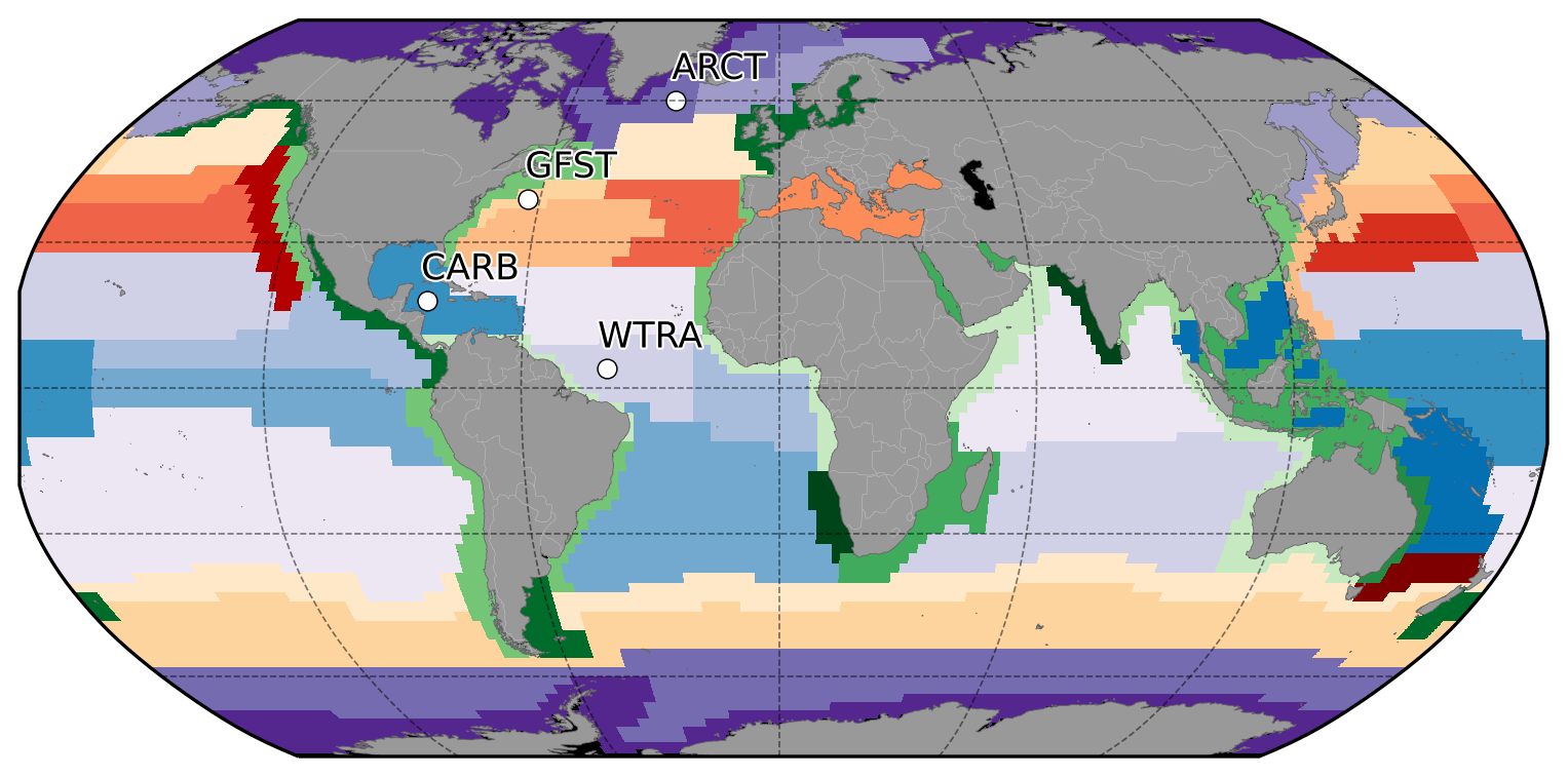
Figure 1Biogeochemical provinces according to Longhurst (2007). Purple shades denote the polar biome, red–yellow the westerlies biome, blue the trades biome, and green the coastal biome. Regions analyzed in detail in this paper are identified by the codes ARCT (Atlantic Arctic province), GFST (Gulf Stream province), WTRA (western tropical Atlantic province), and CARB (Caribbean province).
2.2 The Darwin-CBIOMES-0 physical–biogeochemical–optical model
We use output from a coupled physical–biogeochemical–optical model adapted and configured for the Simons Collaboration on Computational Biogeochemical Modeling of Marine Ecosystems (CBIOMES) project. The model configuration, hereafter denoted as Darwin-CBIOMES-0 (Dutkiewicz, 2018), is global and simulates the period 1992–2006 (Forget and Ferreira, 2019). The physical component uses the MITgcm (Campin et al., 2020) in a three-dimensional global configuration developed as part of the Estimating the Circulation and Climate of the Ocean project (Forget et al., 2015; Forget and Ponte, 2015; ECCOv4). The state estimate uses a least squares with Lagrangian multipliers approach to adjust the internal model parameters, in addition to the initial and boundary conditions with global observational data streams, including satellite altimetry and Argo floats. The resolution is nominally 1∘ in the horizontal and ranges from 10 m in the vertical at the surface to 500 m at depth (see Forget et al., 2015, for details).
The biogeochemical component resolves the cycling of carbon, phosphorus, nitrogen, silica, iron, and oxygen through inorganic, living, dissolved, and particulate organic phases. The ecosystem incorporates 35 phytoplankton and 16 zooplankton types, as in Dutkiewicz et al. (2021). The phytoplankton include several biogeochemical functional groups. Diatoms (that utilize silicic acid), coccolithophores (that calcify), mixotrophs (that photosynthesize and graze on other plankton), nitrogen-fixing cyanobacteria (diazotrophs), and picophytoplankton. Each group has a range of size classes, such that the phytoplankton span from 0.6 to 228 µm equivalent spherical diameter (ESD). Several phytoplankton parameters, including maximum growth rate, nutrient affinity, and sinking are expressed as functions of the cell volume, though with distinct differences between functional groups, as suggested by observations (Dutkiewicz et al., 2020b; Sommer et al., 2017). The 16 size classes of zooplankton range from 6.6 to 2425 µm ESD and graze on (phyto- or zoo-)plankton 5 to 20 times smaller than themselves but preferentially 10 times smaller (Hansen et al., 1997; Kiørboe, 2019; Schartau et al., 2010) with a Holling's type III parameterization (Holling, 1959). The simulation uses Monod kinetics, and stoichiometries are constant over time (though they differ between phytoplankton groups). We refer the reader to Dutkiewicz et al. (2015, 2020b, 2021) for a further description of the model, in addition to an evaluation of the modeled plankton size class and functional group distributions. Here we focus instead on the model Chl concentrations. Each of the 35 phytoplankton types have dynamic Chl that alters as a function of light, nutrients, and temperature, following Geider et al. (1998). Chlmod refers to the sum of modeled Chl across all the phytoplankton types.
The optical component of the model includes an explicit radiative transfer of spectral irradiance in 25 nm bands between 400 and 700 nm. The three-stream (downward direct, Ed, downward diffuse, Es, and upwelling, Eu) model (following Aas, 1987; Gregg, 2002; Gregg and Casey, 2009) is reduced to a tridiagonal system that is solved explicitly (see Dutkiewicz et al., 2015, for more details). In-water irradiance fields are altered by the spectral absorption and scattering by water molecules, the 35 phytoplankton types, detritus, and colored dissolved organic matter (CDOM). Irradiance just below the surface of the ocean (direct, Edo, and diffuse, Eso, downward) is provided by the Ocean–Atmosphere Spectral Irradiance Model (Gregg, 2002; Gregg and Casey, 2009; OASIM).
Output from the optical model includes spectral surface upwelling irradiance similar to that measured by ocean color satellites (Dutkiewicz et al., 2018, 2019). As in these earlier studies, we calculate model reflectance for each waveband as the upwelling just below the surface (Eu) divided by the total downward (direct and diffuse) irradiance also just below the surface (as provided by OASIM) as follows: . We first convert the model subsurface irradiance reflectance to remotely sensed reflectance just below the surface, using a bidirectional function Q as follows: , where we assume that Q=3 sr (as in Dutkiewicz et al., 2019; Gregg, 2002). Second, we convert to above-surface remotely sensed reflectance using the formula of Lee et al. (2002) as follows: . These spectral fields will be referred to as model Rrs (units of sr−1), and this is comparable to the Rrs provided by ocean color satellite databases.
An advantage of having the model Rrs is that we can provide a model-derived satellite-like Chl similar to that described in the previous section (see Dutkiewicz et al., 2018, 2019). In practice, we interpolate the 13 wavebands of Rrs from the model to the same bands as used in OC-CCI and use the maximum ratio of the blue signal to the green and a fourth-order polynomial to estimate the satellite-like-derived Chl (following O'Reilly et al., 1998). Here, for simplicity, we use the OC version 2 algorithm and coefficients. This product is termed ChlRrs in this paper and is technically more comparable to the real-world satellite product than the model's actual Chl at the surface (Chlmod; see the further discussion in Dutkiewicz et al., 2018). Any pixels with invalid data in the satellite product after downscaling to the model grid are masked in the corresponding model output.
2.3 Satellite-derived chlorophyll
The model is compared to satellite-derived Chl products originally at 4 km resolution from version 4.2 of the Ocean Colour Climate Change Initiative (Mélin et al., 2017; Sathyendranath et al., 2019, 2020; OC-CCI). This is a blended Chl product, where data from the Sea-viewing Wide Field-of-view Sensor (SeaWiFS), Aqua Moderate Resolution Imaging Spectroradiometer (MODIS-Aqua), Medium Resolution Imaging Spectrometer (MERIS), and Suomi National Polar-orbiting Partnership Visible Infrared Imaging Radiometer Suite (NPP-VIIRS) products are merged into a unified product. SeaWiFS operated from September 1997 until December 2010 and MERIS from March 2002 to May 2012. MODIS-Aqua was launched in May 2002 and VIIRS in October 2011; the latter two sensors are still operational as of December 2021. Data from the different instruments are merged after band-shifting normalized remote sensing reflectance (Rrs) to the spectral bands of SeaWiFS and correcting for intersensor biases. Atmospheric correction is performed using Polymer v3.5 (Steinmetz et al., 2011) for MERIS and MODIS-A and NASA's SeaDAS 7.3 for SeaWiFS and VIIRS. All individual grid cells are classified optically using a fuzzy-logic approach (Moore et al., 2009, 2012; Jackson et al., 2017), and a combination of the best Chl algorithms for each class is used along with class membership at each pixel to generate Chl at each pixel. The spatial mapping follows NASA's protocol for level-3 processing by considering a 4 km bin as valid if there is at least a single 1 km valid pixel in that bin from at least one sensor and taking the mean if more than one valid observation is available. The resulting time series for the period between 1997 and 2019 is designed to be internally consistent (all radiometric products are band-shifted to a common set of bands corresponding to SeaWiFS) and stable (corrected for intersensor bias Sathyendranath et al., 2019). The resulting daily 4 km OC-CCI product is downscaled to the Darwin-CBIOMES-0 grid using bucket resampling from the satpy resampling package (Raspaud et al., 2019) in Python. We henceforth denote the Chl product from OC-CCI as Chlsat in the study.
2.4 In situ data
The satellite-derived and simulated Chl concentrations are matched with ∼ 80 000 in situ Chl observations for comparison. The in situ Chl data set is based on a global compilation developed to evaluate the quality of ocean color satellite data records and to evaluate ocean color products from OC-CCI (Valente et al., 2019a). The observations were acquired from several sources. The data set spans the period from 1997 to 2018, and variables include spectral remote sensing reflectances, concentrations of Chl, spectral inherent optical properties, spectral diffuse attenuation coefficients, and total suspended matter. Different methodologies have been implemented for the homogenization, quality control, and merging of all data. Observations close in time and space are averaged, and some data were eliminated after failing quality control. To be consistent with satellite-derived Chl values, which are derived from the light emerging from the upper layer of the ocean, all observations in the top 10 m (replicates at the same depth or measurements at multiple depths) were averaged. Data points are discarded if the coefficient of variation among observations is more than 50 %. The compiled in situ data set is publicly available (Valente et al., 2019b). The resulting data product is referenced to here as Chlobs.
2.5 Statistical analysis
While the objective of this study is to assess different continuous probability distributions of Chl, we perform all statistical analyses by converting the distributions to discrete histograms, where the data are divided into equally sized bins on a log scale. The reason for using a log scale is that Chl concentrations can be assumed to follow a lognormal distribution at a variety of spatial and temporal scales (Campbell, 1995), and this transformation allows for better characterizations at low concentrations. We use the same set of 100 equally sized bins from −6.9 (ln 0.001) to 4.61 (ln 100) for all data sources and in all calculations. The histograms are generated by binning daily interpolated Chl from both the satellite (derived Chl from OC-CCI) and Darwin-CBIOMES-0 output by month and Longhurst province for the period 1998 to 2007. The in situ data set has very few, if any, observations in several provinces and is only used for comparisons on global or biome scales. Percentiles, medians, standard deviations (SDs), and other statistics are all calculated from the resulting histograms using specifically developed code.
2.5.1 Earth mover's distances
We leverage Earth mover's distance (Rubner et al., 2000; EMD) to quantify the difference between different distributions. EMD, also known as the Wasserstein metric in mathematics (Vaserstein, 1969) and Mallows' distance in statistics (Levina and Bickel, 2001), is a popular optimal transport method (Monge, 1781) for measuring the distance between two probability distributions and is widely used in image processing (Frogner et al., 2015) and scientific applications (Orlova et al., 2016). The distance is based on imagining a mound of dirt shaped like the first distribution and considering how much effort would be required to transform it to the second distribution's shape. Given a distance metric in this space (in this case, the absolute difference in log Chl), it is possible to calculate the minimum redistribution of mass needed to transform one probability distribution to the other. EMD measures the total sum of such an optimally planned transfer of mass. Rather than focusing on the distance between any particular aspect of the distributions, such as their means or variances, EMD provides a more comprehensive measure of the distance. For computation, the original log Chl measurements in each province are transformed into histograms using the earlier-mentioned bin definitions. We use the Python package PyEMD (Pele and Werman, 2008, 2009; Mayner et al., 2015) to calculate EMDs between the histograms. All reported EMDs have the natural log of Chl as the unit.
3.1 Taylor diagrams
Taylor diagrams (Taylor, 2001) based on different spatial and temporal aggregations of satellite and model chlorophyll concentrations reveal different model bias patterns at different scales of averaging (Fig. 2). These diagrams are polar representations of pairwise statistics between Chlsat, Chlmod, and ChlRrs, with the correlation coefficient as the angle and the SD of Chlmod or ChlRrs normalized to Chlsat as the radius. Each individual data point represents the SD and correlation for a specific Longhurst province, different colors denote different basins, and different marker shapes denote different biomes. Figure 2a–b shows the resulting diagram based on daily match-ups for individual grid cells in the model versus satellite data reprojected to the model grid. Each symbol shows the point-by-point statistics within a Longhurst province. We find the correlation to generally be quite low (R=0–0.5) for all Longhurst provinces, and the model SD is 0.5 to 1.8 times Chlsat. This skill metric could be highly affected by small mismatches and lags in time and space between the model and satellite data. We utilize the assumption that a given Longhurst province is controlled by a specific combination of physical, chemical, and biological process by averaging ChlRrs, Chlsat, and Chlsat over all grid cells in each province for each day and presenting the resulting data set as Taylor diagram (as seen in Fig. 2c–d). Some Longhurst provinces show a better correlation (R>0.8), whereas others have a negative correlation between satellite-derived Chl and model output. Model SD scaled to satellite data also shows more variability between provinces when compared with individual grid cells. While aggregating the data over Longhurst provinces dampens random spatial errors, temporal fluctuations at the daily scale are still present. In Fig. 2e–f, we show a Taylor diagram using monthly time series instead of the daily time series used for Fig. 2c–d and find a much clearer separation between the Longhurst provinces. Some provinces are highly correlated, while others are showing negative correlations. The latter patterns could be explained by the more aggregated data sets having less random noise, which lets systematic mismatches be more visible and thus detected by the Taylor diagram. We find that Chlmod points generally have a slightly more pronounced spread and hence more variability in the misfit than ChlRrs.
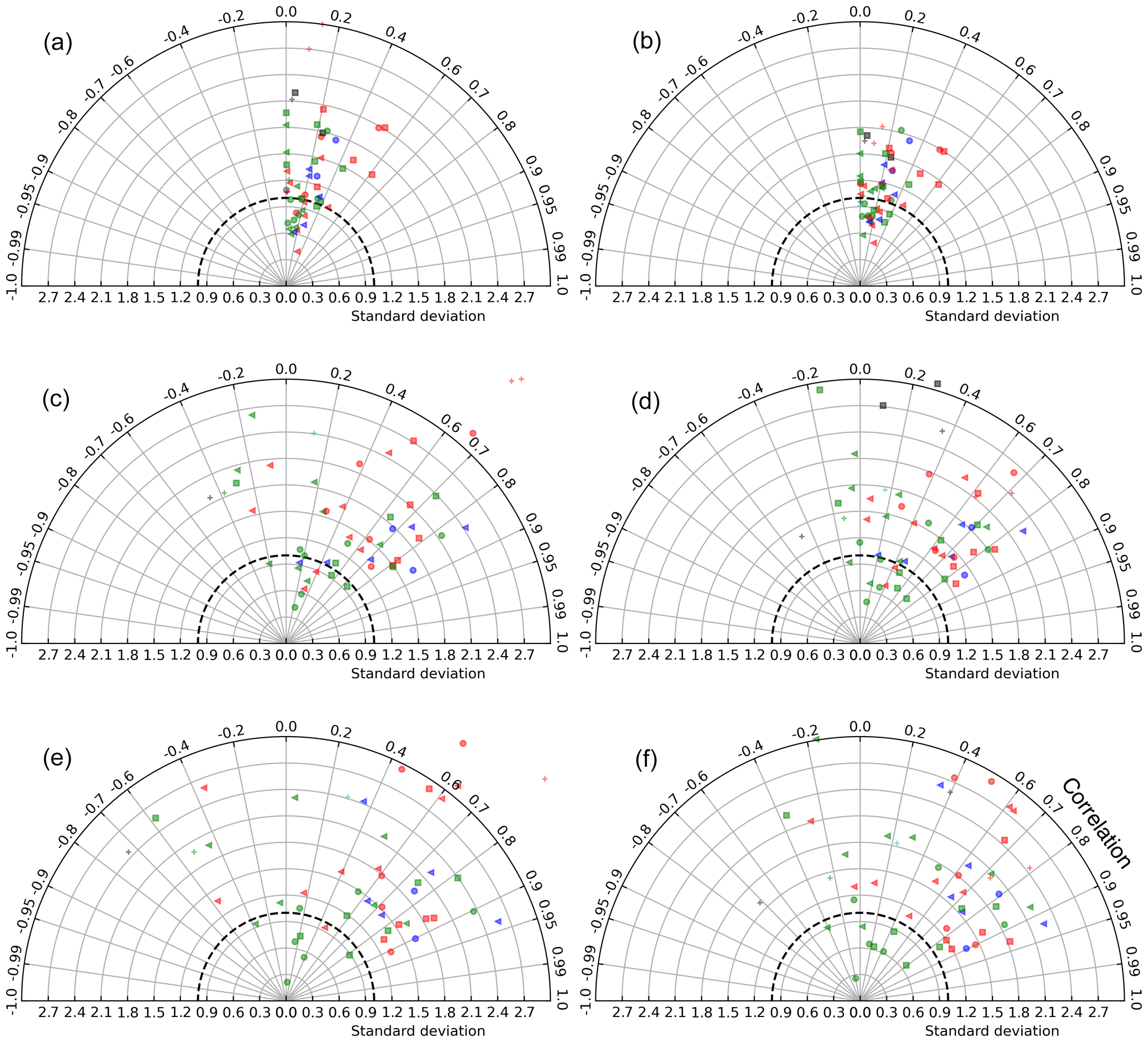
Figure 2Taylor diagrams based on comparisons between satellite-derived OC-CCI Chl (Chlsat) and Chl concentrations from the Darwin-CBIOMES-0 configuration (ChlRrs). Each point represents a Longhurst province. The model standard deviation is normalized to satellite data (thick dashed line). Different colors denote different basins, so that cyan is the Arctic Ocean, red is the Atlantic Ocean, blue is the Indian Ocean, green is the Pacific Ocean, and black is the Southern Ocean. Different marker shapes denote different biomes, so that the triangle is the coastal, the plus sign is polar, the circle is trades, and the square is westerlies. (a) Point-by-point comparison between Chlsat and Chlmod, where daily match-ups and each grid cell in the model and satellite products are used. Panel (b) is the same as panel (a) but for Chlsat and ChlRrs. (c) Daily match-ups between Chlsat and Chlmod, but all data falling within a Longhurst region are averaged to one value for each day for each Longhurst region. Panel (d) is the same as panel (c) but for Chlsat and ChlRrs. (e) The daily time series in panel (a) are further aggregated to monthly averages for match-ups between Chlsat and Chlmod. Panel (f) is the same as panel (e) but for Chlsat and ChlRrs.
3.2 Global distributions
Global distributions of Chlobs, Chlsat, Chlmod, and ChlRrs show that distributions of satellite-derived Chl and in situ observations are very similar, but Darwin-CBIOMES-0-based Chl shows a systematic bias (Fig. 3). Histograms of Chlobs and Chlsat are shown in Fig. 3a and b. Only data pairs for which both Chlobs and Chlsat have valid values are used (35 174 match-ups out of 80 524 observations). We find the in situ and satellite data sets to have similar distributions without any significant biases in Chlsat. Note that some of the Chl algorithms contributing to the final Chlsat product would have been tuned, using a small subset of the in situ database, and corresponding in situ or satellite-derived Rrs (other than the OC-CCI products). Similarly, the algorithm used to provide ChlRrs from the Darwin-CBIOMES-0 output (O'Reilly et al., 1998) would have used a subset of the in situ data set along with measured Rrs values to calibrate the algorithm. But none of the observations in the in situ data sets has been used to tune either the OC-CCI products or the Darwin-CBIOMES-0 outputs.
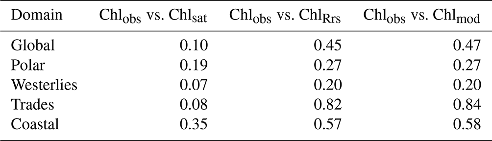
Whereas Chlobs closely follows a lognormal distribution, Chlsat shows some divergence from the expected distribution. The pronounced secondary peak at about 5 mg m−3 is related to coastal provinces, and the broader peak at 0.5 mg m−3 represents values from the subtropical gyres. In Fig. 3b, Chlsat has thinner tails than Chlobs, and the distribution is more centered around the median. This pattern is consistent with our expectations, since Chlsat has a coarser resolution (4 km) than Chlobs (the volume of each sample). One can expect a spatially aggregated measurement to have fewer extreme values. Panels c and d in Fig. 3 are analogous to panels a and b but with Chlmod and ChlRrs included. Here, the collocation between all four sources is required, which results in 20 935 match-ups. The differences in the distributions of Chlobs and Chlsat in Fig. 3c and d compared with Fig. 3a and b occurs from the shorter time span of the Darwin-CBIOMES-0 configuration (1998–2006) compared with the OC-CCI time domain (1998–2020) and from the masking out of near-coastal locations. The model grid also has a coarser resolution (≈1∘) than the satellite product. The four-way match-up (Fig. 3c and d) allows us to compare the different data sources in a reasonably objective way by considering both seasonal variability and data density. We find that the global distributions of Chlmod and ChlRrs are nearly identical to each other but significantly different from both Chlobs and Chlsat. It is clear that Darwin-CBIOMES-0 systematically generates lower Chl concentrations than either the satellite-derived product or in situ observations do. It is somewhat nonintuitive that the model has similar or longer tails than Chlobs or Chlsat, especially considering the model's coarser spatial resolution and the earlier comparison between satellite and in situ Chl. EMDs calculated for Chlobs vs. Chlsat, ChlRrs, and Chlmod, respectively (Table 1), confirm these findings with much larger (and similar) distances for ChlRrs and Chlmod than Chlsat. These dissimilar EMDs are the combined result of differences in medians, SD, and skewness between the model and observations.
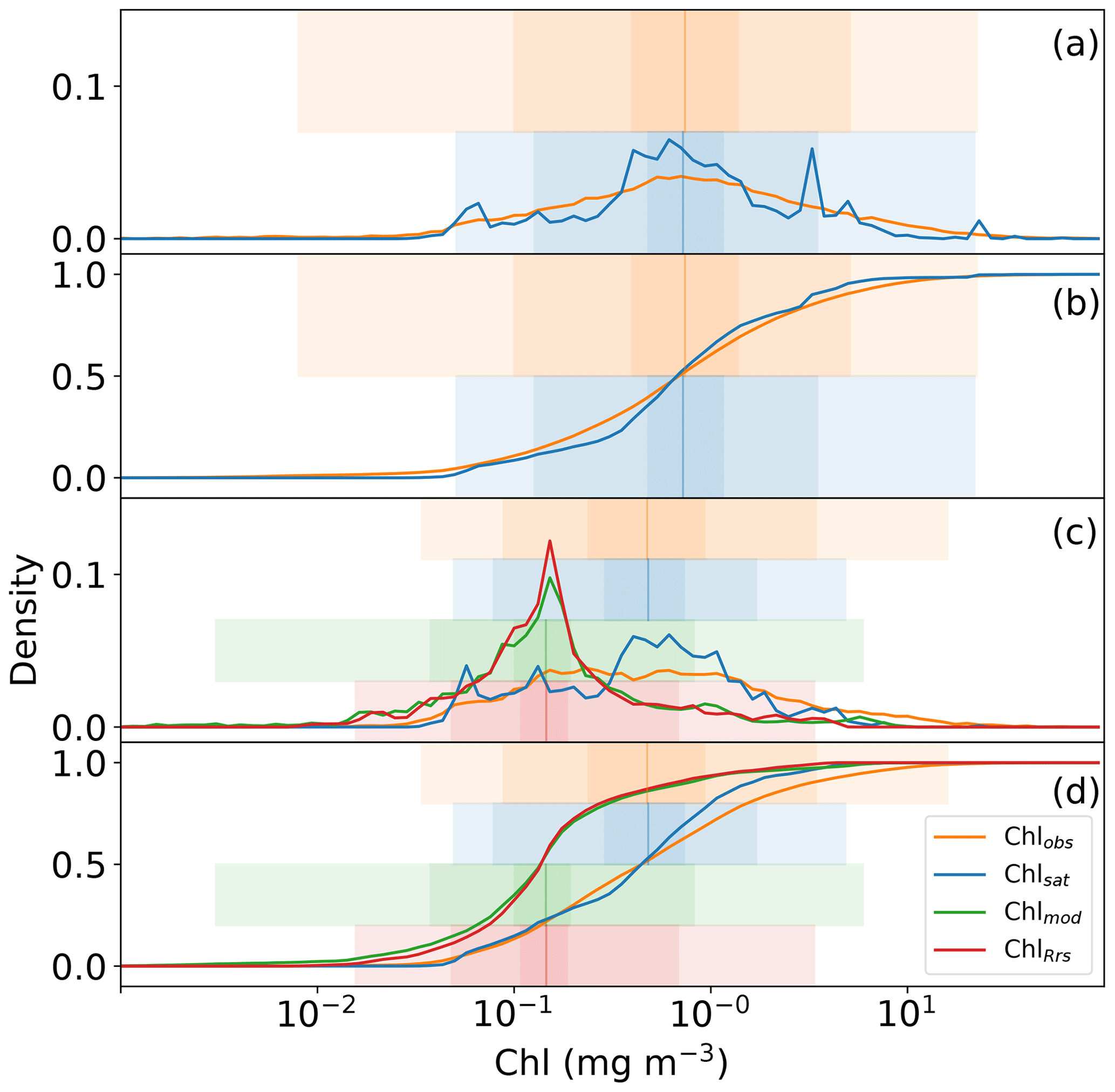
Figure 3Distributions of in situ (Chlobs), satellite-derived (Chlsat), and modeled (Chlmod) chlorophyll (Chl) and Chl derived from simulated remote sensing reflectances in the Darwin-CBIOMES-0 configuration (ChlRrs). All data sets are matched in time and location, and only complete match-ups are used. Shadings show the 1 %–99 %, 10 %–90 %, and ±1σ percentiles in the respective distributions. (a) The respective histograms of Chlobs (orange line) and Chlsat (blue line). (b) The corresponding cumulative distribution. Panels (c) and (d) are analogous to panels (a)–(b) but with Chlmod (green lines) and ChlRrs (red lines). Note that the data sets for Chlobs and Chlsat differ between panels (a)–(b) and panels (c)–(d) due to the smaller coverage in the temporal range of Darwin-CBIOMES-0.
While the distributions of Chlmod and ChlRrs are close to identical, there is much more variability between the two properties when compared on a point-by-point basis. Figure 4, panel a, shows a 2D histogram of Chlmod and ChlRrs sampled from the model at the same time and grid cell. While most values fall close to the 1:1 line, there is a large spread. The 95 % confidence interval of the residual is about 2 orders of magnitude. These results show the importance of diagnosing the model using a metric that is comparable to Chlsat. Any divergence from the 1:1 line in Fig. 4 a could incorrectly be interpreted as model misfit.
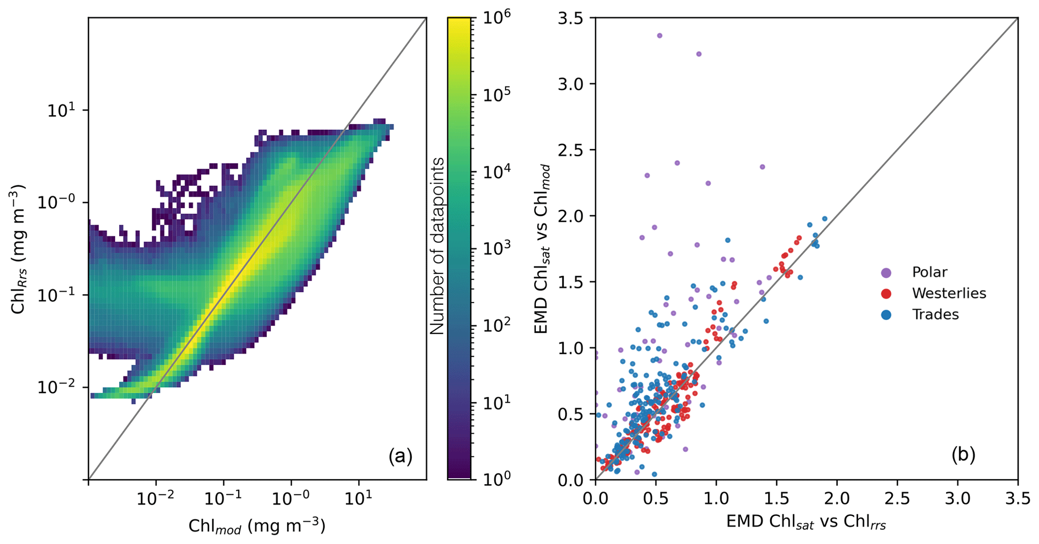
Figure 4(a) Point-by-point comparisons of satellite-derived (Chlsat) and modeled (Chlmod) chlorophyll. Colors denote the number of data points in that bin. (b) Earth mover's distances for each province and month calculated using Chlsat and either Chlmod or Chl derived from simulated remote sensing reflectances in the Darwin-CBIOMES-0 configuration (ChlRrs). Purple denotes the polar biome, red the westerlies biome, and blue the trades biome. The coastal biome is omitted as per the description in the main text.
3.3 Distributions in different biomes
As the global distributions show only general biases between Darwin-CBIOMES-0, in situ, and satellite-derived Chl, we divide the data into biomes based on Longhurst (2007) to better understand the misfits. Conclusions about model performance will be different if the shift in the probability distributions is caused by errors which are global or limited to specific regions of the ocean. First, we compare EMDs calculated using ChlRrs and Chlmod for each month and province, as shown in Fig. 4b. We find that Chl distributions from the Longhurst provinces in the westerlies biome are similar, but provinces in the trades biome and, particularly, the polar biome show larger EMDs between Chlsat and Chlmod than Chlsat and ChlRrs. Provinces in the coastal biome are omitted here and in the further analysis since Darwin-CBIOMES-0 is not developed to resolve coastal processes.
Figure 5 shows cumulative distributions, analogous to Fig. 3d, for the polar (3741 matches), westerlies (1240 matches), trades (3328 matches), and coastal (12 418 matches) biomes. Mismatches are different for the different biomes, with Chlsat generally following Chlobs more closely than the model does. The general trend of Chlsat having less variance than Chlobs and both Chlmod and ChlRrs having a negative bias is also evident. Chlmod has a much wider distribution in the polar biome than Chlsat or ChlRrs, especially for low concentrations. All distributions show close similarities in the westerlies biome, suggesting that the model has relatively high skill with respect to simulating phytoplankton biomass (for which Chl acts as a proxy) in this biome. The largest mismatch between the model and observations is in the coastal biome; this is something which is to be expected when considering the spatial resolution of the model. This biome is also where Chlsat shows the largest inconsistencies compared to Chlobs. Coastal areas tend to have more complex case II waters, where Chl algorithms are more affected by colored dissolved organic matter (CDOM) or total suspended matter (TSM; Morel and Prieur, 1977; Lee and Hu, 2006).
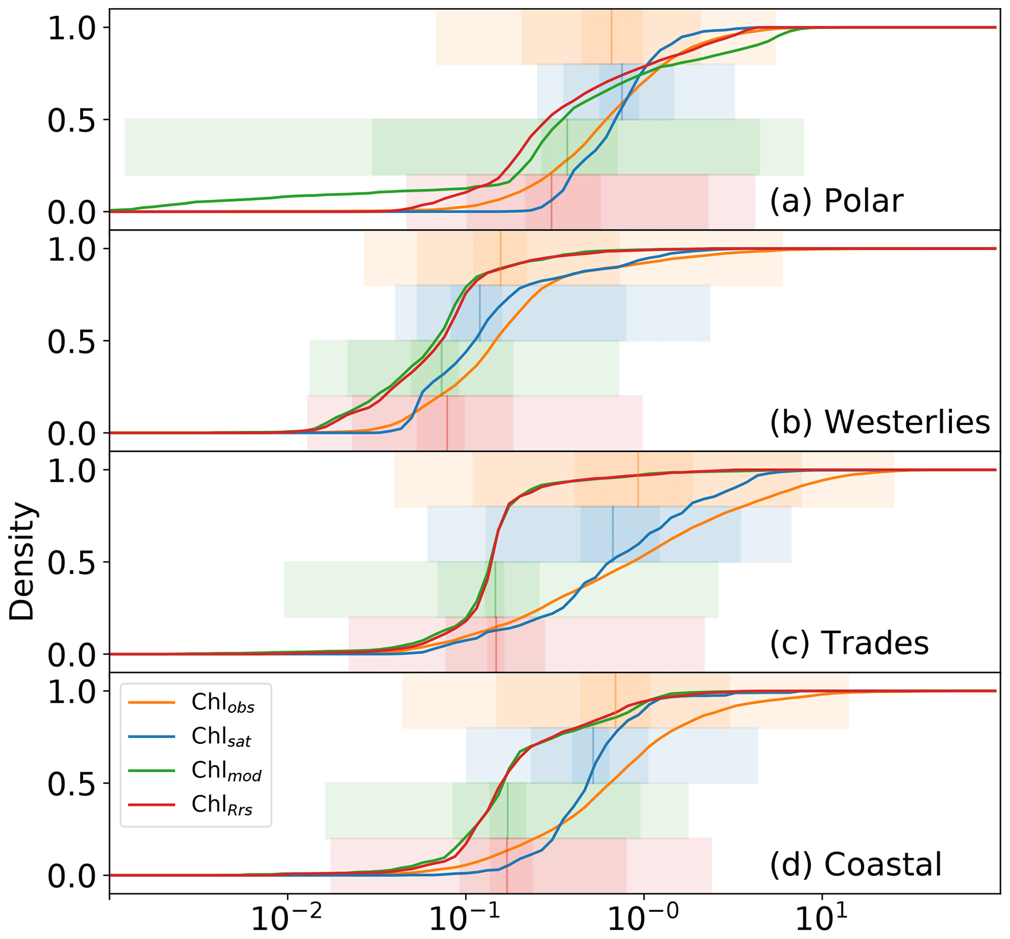
Figure 5Distributions of in situ (Chlobs), satellite-derived (Chlsat), and modeled (Chlmod) chlorophyll (Chl) and Chl derived from simulated remote sensing reflectances in the Darwin-CBIOMES-0 configuration (ChlRrs) for each of Longhurst's biomes. All data sets are matched by time and location, and only match-ups in which data from all four sources are present are used. Shadings show the 1 %–99 %, 10 %-90 %, and ±1σ percentiles in the respective distributions. (a) Cumulative distributions for match-ups located in provinces in the polar biome, as defined by Longhurst (2007). (b) Analogous distributions for data in the westerlies biome, (c) data for the trades biome, and (d) data for provinces in the coastal biome.
Table 1Earth mover's distances comparing distributions of in situ (Chlobs), satellite-derived (Chlsat), and modeled (Chlmod) chlorophyll (Chl) and Chl derived from simulated remote sensing reflectances in the Darwin-CBIOMES-0 configuration (ChlRrs). See Fig. 1 for the extent of each biome.
3.4 Individual Longhurst provinces
We extend the study to individual Longhurst provinces to further explore differences between the model and satellite-derived observations. The limited geographical and seasonal coverage of in situ data limits our ability to include Chlobs, so we therefore focus on comparing Chlsat with Chlmod and ChlRrs in the following section, while conceding the limitations of the approach. Chlsat, for example, probably underestimates the variance in Chlobs but is at the same time more representative of the reduced variance within large model grids. We exclude coastal provinces from the analyses, since the model is not expected to have as much skill near land or in shallow waters, due to the relatively coarse vertical and horizontal grid resolution discussed earlier and the challenges with satellite retrieval of Chl in coastal waters. We still find interesting patterns when comparing Chl distributions in individual open-ocean Longhurst provinces.
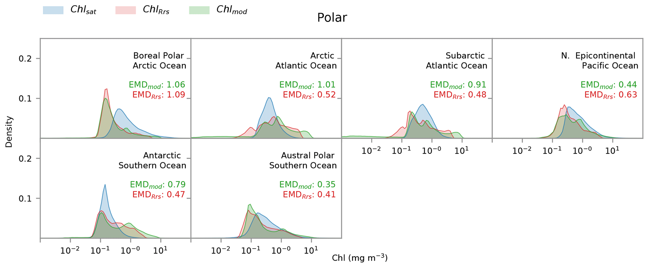
Figure 6Distribution of satellite-derived (Chlsat – blue) and modeled (ChlRrs – red; Chlmod – green) chlorophyll for different Longhurst provinces in the polar biome. Red values are the Earth mover's distances (EMDs) between the Chlsat and ChlRrs distributions, and green values are the EMDs between the Chlsat and Chlmod distributions.
Individual histograms for Longhurst provinces in the polar biome often show stark differences between Darwin-CBIOMES-0 and OC-CCI, as seen in Fig. 6. The very low Chl concentrations seen in the polar biome (Fig. 5) for the Chlmod distribution primarily occur in the boreal polar, Arctic, and subarctic sections of the Atlantic Ocean (Fig. 6). The Arctic section of the Pacific Ocean shows a small bias towards low values as well but is much less extreme. Chl concentrations are biased low in Darwin-CBIOMES-0 close to the Antarctic continent (austral polar province) but biased high towards the Antarctic Circumpolar Current (Antarctic province). This pattern could suggest a meridional misalignment of physical processes that drive Chl variability in the Antarctic Ocean. Since the comparisons are carried out only for match-up data where satellite and model data are available, the differences observed here cannot be explained as a consequence of the poor sampling of the polar biome by satellites due to adverse viewing conditions, especially in winter (Jönsson et al., 2020b).
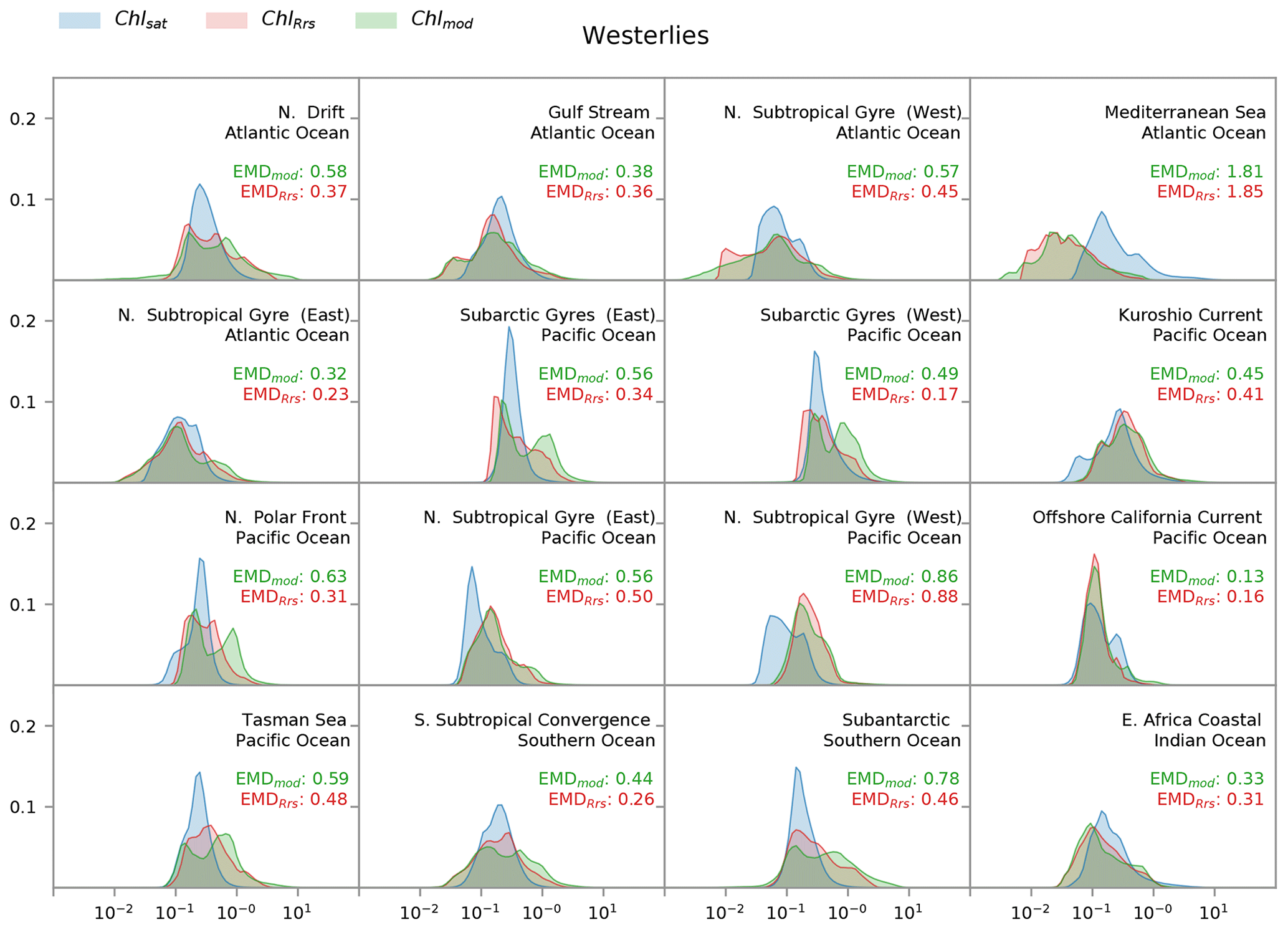
Figure 7Distribution of satellite-derived (Chlsat – blue) and modeled (ChlRrs – red; Chlmod – green) chlorophyll for different Longhurst provinces in the westerlies biome. The east Africa coastal province is included, as it contains the Agulhas current. Red values are the Earth mover's distances (EMDs) between the Chlsat and ChlRrs distributions, and green values are the EMDs between the Chlsat and Chlmod distributions.
Whereas Fig. 5 shows a strong correspondence between Chlsat and ChlRrs in the westerlies biome, we find a more complicated picture in the individual Longhurst provinces within this biome (Fig. 7). In most provinces, Chlsat and ChlRrs have similar medians, but the tails are often significantly different. Chl concentrations in the Darwin-CBIOMES-0 configuration are biased towards high values in most provinces in the Pacific Ocean and the Southern Ocean. ChlRrs also tends to have a bimodal distribution in contrast to the expected lognormal distribution of Chlsat. There is also a clear negative bias in ChlRrs in the Mediterranean Sea, which may indicate that the model resolution is too coarse to resolve all the hydrodynamics in this small but very complex sea.
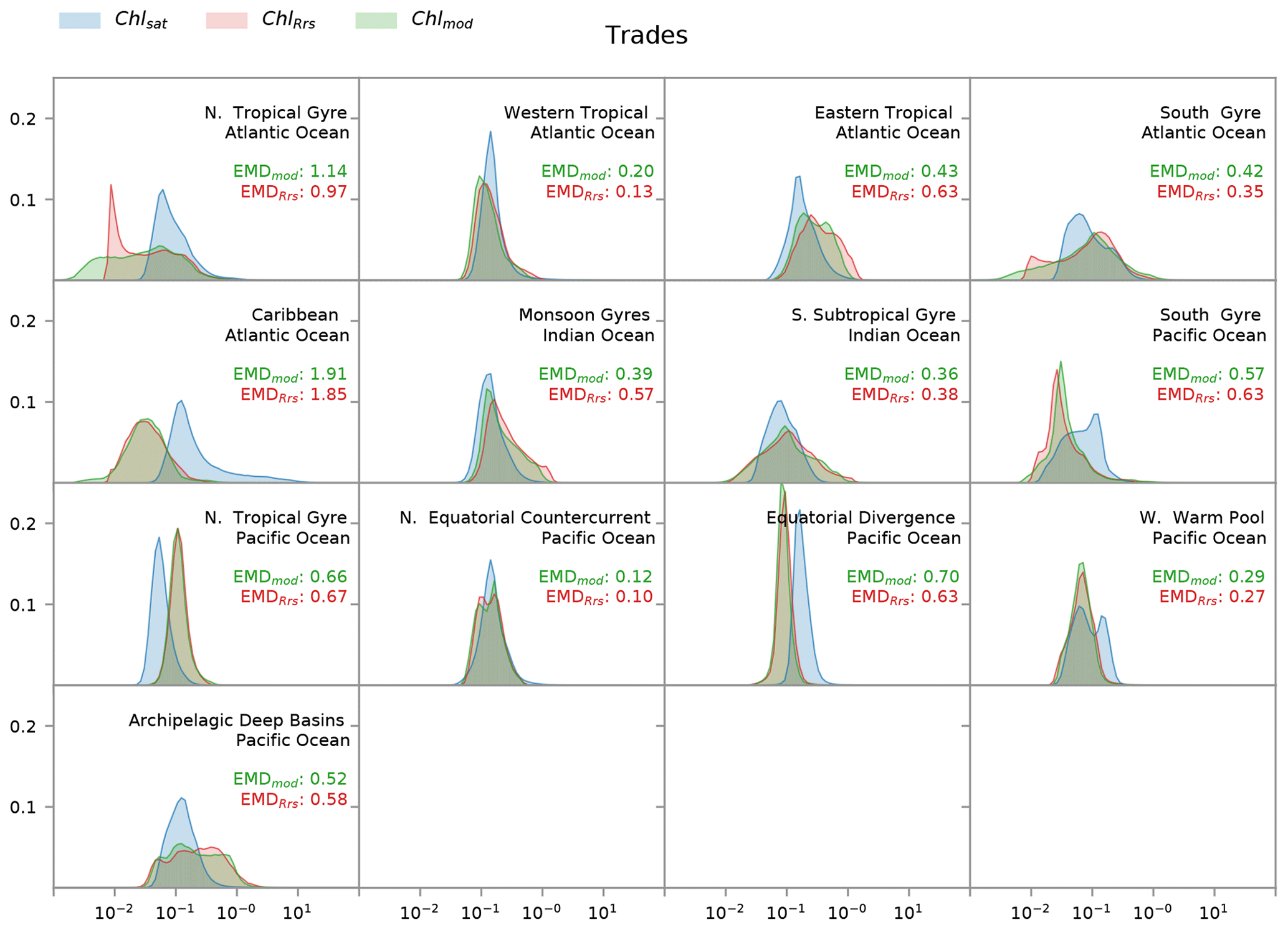
Figure 8Distribution of satellite-derived (Chlsat – blue) and modeled (ChlRrs – red; Chlmod – green) chlorophyll for different Longhurst provinces in the trade winds biome. Red values are the Earth mover's distances (EMDs) between the Chlsat and ChlRrs distributions, and green values are the EMDs between the Chlsat and Chlmod distributions.
Longhurst provinces in the trades biome generally show similar distribution widths and shapes of Chlsat and ChlRrs, aside from biases in the medians (Fig. 8). The main outliers are the northern tropical gyre in the Atlantic Ocean and the archipelagic deep basin in the Pacific Ocean, where ChlRrs has a rectangular or weakly bimodal distribution. The western warm pool and south gyre in the Pacific Ocean also stand out as the only two provinces where Chlsat has a bimodal distribution and ChlRrs does not.
3.5 Monthly distributions
By extending the analysis to monthly distributions for each Longhurst province, we can identify the temporal differences between OC-CCI and Darwin-CBIOMES-0. The large number of resulting probability distributions is challenging to present, and we only show a few interesting examples here. Figures for all provinces are provided with the associated data sets described in the acknowledgements. Figure 9 shows the graphical representations of probability distributions for some representative provinces in the North Atlantic Ocean, generated by aggregating daily Chlsat, ChlRrs, and Chlmod by climatological month. The largest intra-annual differences are found in provinces in the polar biome, as exemplified by the Atlantic Arctic province (Fig. 9a), where Chlmod shows much lower concentrations and much more variability than either Chlsat or ChlRrs during the winter and spring months. All three data products have similar distributions and progressively smaller variability during the summer. But Chlsat shows both a significant drop in concentrations and an increase in variability in November, and this is not seen in ChlRrs or in Chlmod.
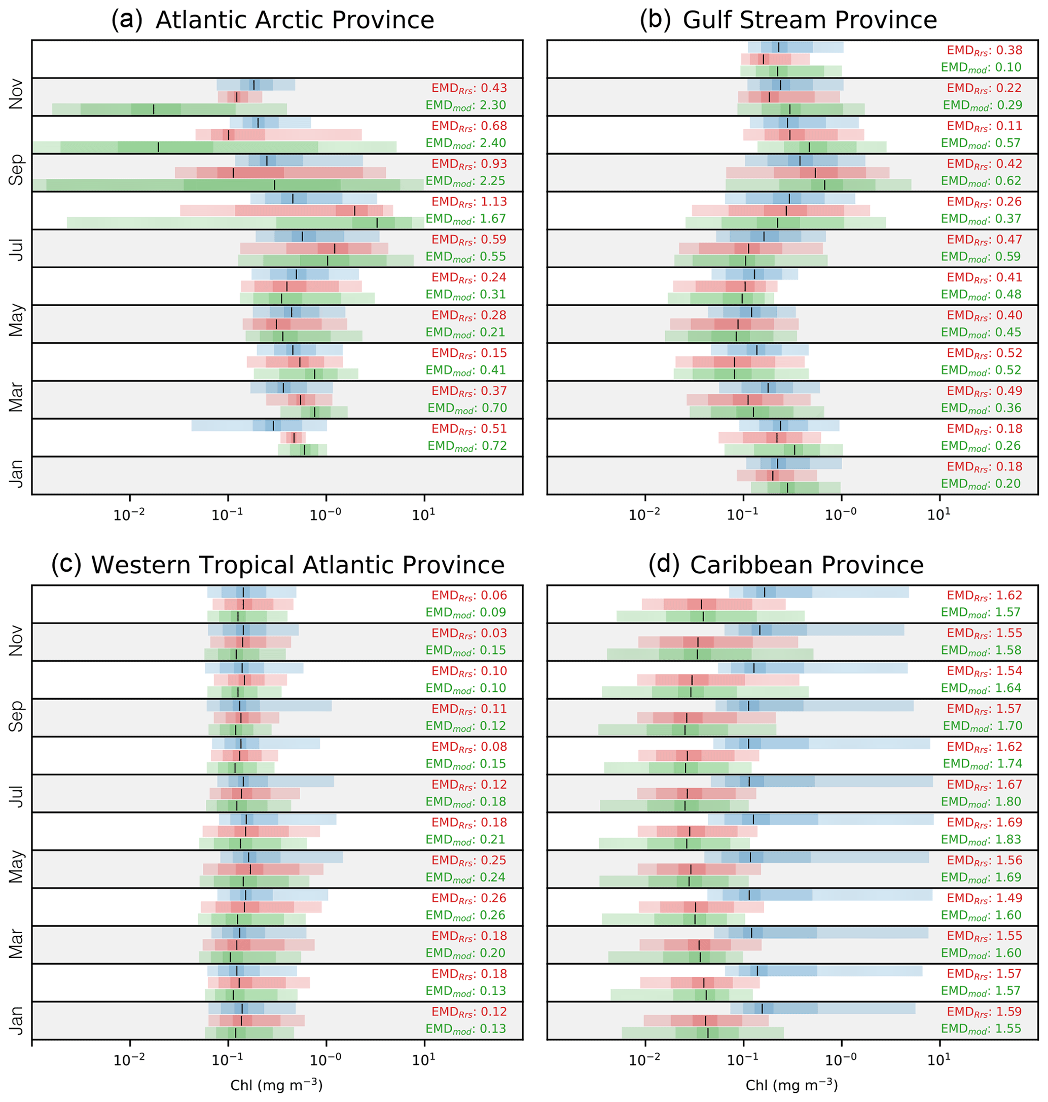
Figure 9Monthly distributions of satellite-derived (Chlsat – blue), model-derived Rrs (ChlRrs – red), and simulated Chl (Chlmod – green). Shadings show the 1 %–99 %, 10 %–90 %, and ±1σ percentiles in the respective distributions. Vertical black lines denote the medians. (a) A representation of the polar biome's Atlantic subarctic province, (b) the westerlies biome's Gulf Stream province, (c) the trades biome's western tropical Atlantic province, and (d) the trades biome's Caribbean province. Note that data are not available for January and December due to ice cover and adverse satellite viewing conditions in panel (a). Red values are the EMDs between the Chlsat and ChlRrs distributions, and green values are the EMDs between the Chlsat and Chlmod distributions.
The Gulf Stream province, our chosen example for the westerlies biome, has a distinct seasonal progression, with elevated Chl concentrations during the spring bloom and low values in the summer (Fig. 9b). Both ChlRrs and Chmod generally compare well with ChlRrs but with a negative bias during summer. The model products also tend to have a more stretched out distribution for low values. The good agreement in the seasonal cycle somewhat hides the misfits between the model and satellite observations for individual months.
The two provinces representing the trades biome (the western tropical Atlantic province and the Caribbean province) both show a weak seasonal cycle but very different misfits. The western tropical Atlantic province (Fig. 9c) has a notable similarity in the medians between the different data sources, with the exception that the 99 % percentile for Chlsat is much higher than ChlRrs or Chlmod during spring and summer. This pattern could be interpreted such that processes generating rare bloom events during that time of the year are missing in the Darwin-CBIOMES-0 configuration. The probability distributions of Chlsat in the Caribbean province (Fig. 9d) are notably different from ChlRrs and Chlmod, with both much higher medians and higher 99 % percentiles. This pattern is not unique to the province and can be seen, for example, in the North Atlantic tropical gyre province as well (data not shown). The asymmetric shape of the probability distributions of Chlsat with a high positive skewness is surprising and deserves closer examination in a future study.
3.6 Global and seasonal patterns of Earth mover's distances
The calculated EMD distances between Chlsat and Chlmod or ChlRrs, respectively, for all province–month combinations (partly presented in Fig. 9) are shown as maps in Fig. 10 for two selected months – January and July – using color intensity to depict the EMDs between the two probability density functions for that province–month pair. Here, EMDs provide aggregated information about how different, for example, mean biases, SD, and skewness are in the respective distributions. The global patterns in EMD, when comparing Chlsat with Chlmod or ChlRrs, are quite similar, while the magnitudes are slightly different. This pattern is most pronounced in polar regions.
The ability of EMDs to provide aggregated information about differences between distributions has the consequence that high EMDs can occur for different reasons. To investigate this, we focus our attention on the six province–month pairs with highest EMDs and compare the two Chl distributions as overlaid probability histograms (blue and green lines in Fig. 11). In each of the panels in Fig. 11, the two data sources have visibly different Chl distributions, and it is clear that a large amount of probability mass needs to move for the two data sources to match. Out of the six, the Atlantic Arctic province in March is of particular interest, with the two distributions of Chl having similar means values, while the EMD is very large. This discrepancy is due to a considerable difference in the second or higher moments between the two distributions – the green distribution (Chlmod) has a much higher spread than the blue one (Chlsat). This demonstrates how EMDs can be an effective scalar measure for summarizing the full distributional difference between two data sources.
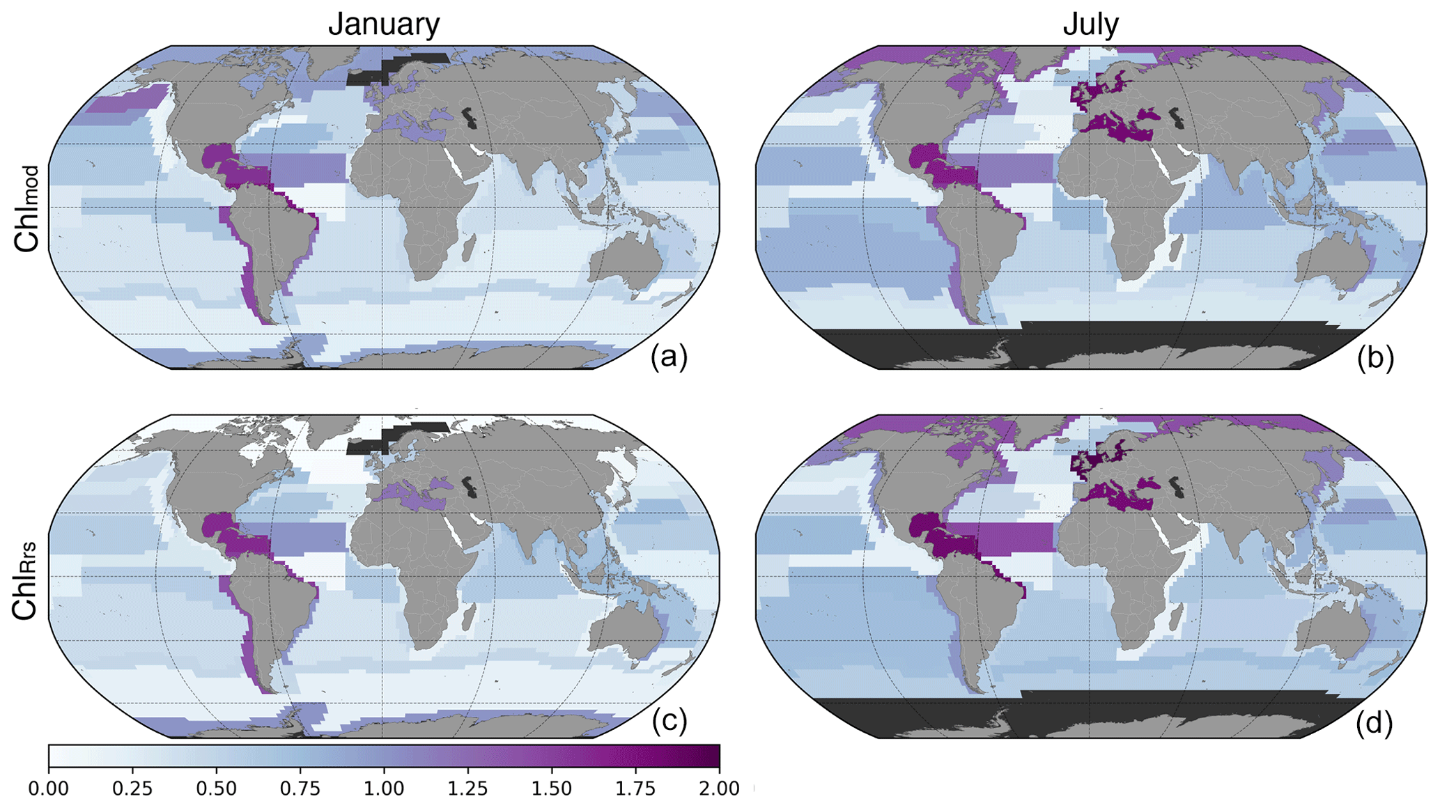
Figure 10Map of Earth mover's distances between Chlsat and Chlmod (a, b) or Chlmod (a, b) for different Longhurst provinces in January (a, c) or July (b, d). The dark gray coloring represents areas where data are not available.
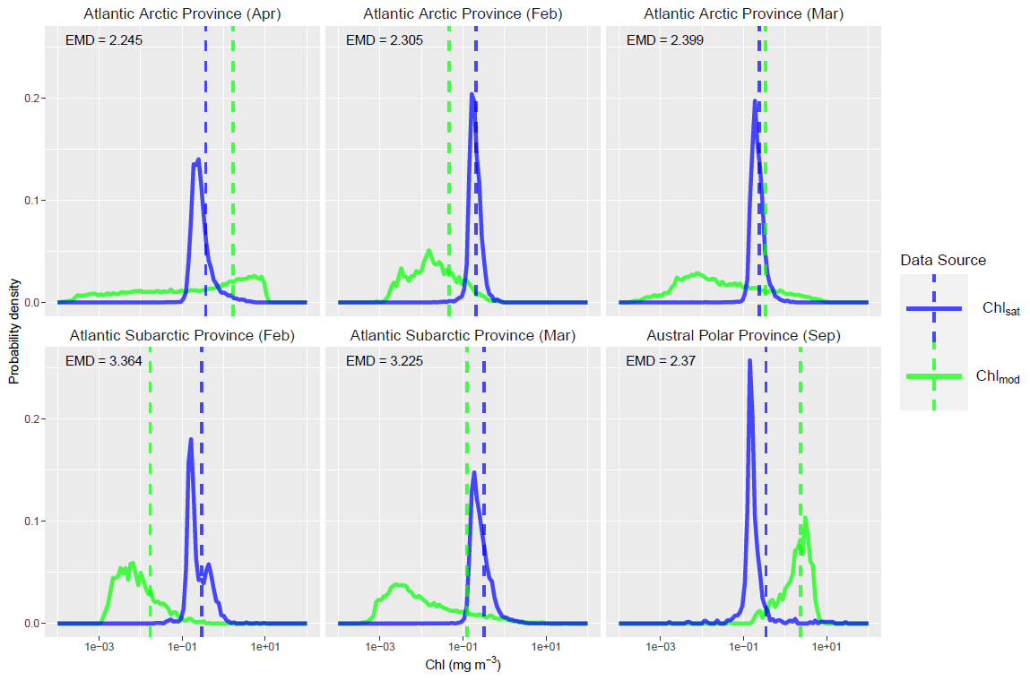
Figure 11Distributions of satellite-derived (Chlsat – blue) and modeled Chl (Chlmod – green) in the top six province–month pairs in terms of Earth mover's distances (EMDs). The vertical dashed lines mark the mean of each distribution. There appears to be a clear distributional difference between the two data sources in each case – a large amount of probability mass would have to be transported from one distribution to another to make the two equivalent. Also notable is that the EMD can be large while the mean difference is small; this highlights how the EMD is a richer measure of the distributional difference.
We combined satellite-derived Chl from OC-CCI with in situ observations and model output from the Darwin-CBIOMES-0 configuration to investigate three new approaches for comparing biogeochemical models and observations. The meant the use of Chl proxies analogous to satellite-derived properties instead of directly diagnosed Chl in the model, the utility of Earth mover's distances (EMDs) as a metric for quantifying differences between distributions, and probability distributions instead of point-by-point comparisons. The first approach has already been presented and evaluated in Dutkiewicz et al. (2018, 2019) as a general tool, and we will focus on its use in the context of comparing distributions.
The main differences between ChlRrs and Chlmod occur on regional scales (Figs. 3–8), particularly in the polar and trades biomes, and these differences generally even out when aggregated over full biomes or globally (Figs. 3–5; Table 1). The differences seen in the polar biome puts earlier results by Jonsson et al. (2015), who argued that the ecosystem models underestimate winter phytoplankton biomass in the Southern Ocean, in a new light. It is possible that the use of ChlRrs and Chlsat as a proxy for phytoplankton biomass is biased in these regions on an inability to detect the low concentrations predicted by the models, which is something that must be further explored with in situ observations. While this issue might seem irrelevant due to the low Chl concentrations, it has large potential effects on the skill with respect to simulating the seasonal progression of polar ecosystems. Order-of-magnitude errors in regions with seasonally low Chl concentrations and large annual variability can be critical when the growth is exponential, thus potentially requiring unrealistically high growth rates (Hague and Vichi, 2018).
ChlRrs is, however, not necessarily a more truthful diagnostic than Chlmod; it is only closer to Chlsat and quite possibly inherits biases from satellite-derived proxies. Another motivation for using ChlRrs as the property of comparison is that Chlmod is poorly defined, since the conversion from a depth-resolved field to a 2D concentration might be performed differently between different models. Our results show that comparisons between Chlmod and Chlsat are generally sufficient if ChlRrs is not available (which is normally the case), as long as these caveats are considered. Figures 6–9 can provide guidance with respect to which regions require the application of caution.
EMDs provide a systematic and quantitative way to assess how the distribution of Chl differs between OC-CCI and the Darwin-CBIOMES-0 configuration. One major application is the ability to compare the likeliness between different distributions in an integrated fashion, as the maps presented in Fig. 10 show. We find that the biggest differences between ChlRrs and Chlmod occur in the polar biome during winter. This pattern is supported by the scatter of EMDs shown in Fig. 4b, where provinces in the polar and trades biomes tend to have larger EMDs for Chlmod than ChlRrs when compared to Chlsat.
When comparing the probability distributions between the Darwin-CBIOMES-0 configuration, OC-CCI satellite-derived Chl product, and in situ observations of Chl, we find many similarities and also important differences. Comparisons between Chlsat and Chlobs (Figs. 3 and 5) show an interesting pattern, where OC-CCI diverges from the expected lognormal distribution with a smaller variance than the set of observations. This difference could be explained by OC-CCI being based on satellite products with overpasses close to noon, thus limiting the ability to resolve the diurnal cycle, and 4 km sized pixels that aggregate the variability at smaller scales. Chlobs data, on the other hand, are sampled at any time over the course of a day and generally represent a water volume of less than 1 m3. A small water volume has a higher chance of having outliers due to patchiness, while a distribution of satellite-derived Chl observations is more clustered around the population mean as a result of averaging many small patches over a larger area. This difference is expected by the law of large numbers. It should also be noted that some of the mismatches between Darwin-CBIOMES-0 and the observations might be partly explained by the unevenness in the temporal and spatial coverage of observations. By only including satellite-derived and modeled Chl concentrations, we are able to minimize potential problems with the temporal and spatial representativeness of in situ observations, since Chlsat is interpolated to the grid of Darwin-CBIOMES-0 and only pixels with valid data in both data sources are used.
While the distributions of Chl in a direct match-up between Chlobs and Chlsat vs. ChlRrs and Chlmod suggest that the model underestimates Chl significantly, regional comparisons provide a more nuanced picture. Data from the westerlies biome have, for example, almost identical distributions. The largest discrepancies are found in coastal areas and the provinces in the polar biome, both of which are notoriously challenging to model due to complex hydrology and large seasonal variability in forcings (light, freshwater run-off from land, nutrient input, etc.). Provinces in the trades biome generally show less variability in the seasonal average but larger differences in the high and low extreme values. These patterns are evident both in the EMD maps seen in Fig. 10 and in the individual histograms seen in Figs. 6–8. Eastern boundary upwelling systems show large discrepancies between ChlRrs and Chlsat. This is to be expected, since these areas are characterized by complex interactions between physical and biological processes over short spatial scales. Other studies have also found that the dominating timescales of variability in these regions are very short, which most global biogeochemical models are not developed to resolve (Jönsson et al., 2023).
Model Chl had long tails with low values in the provinces in the polar biome that might be connected to the Darwin-CBIOMES-0 configuration overestimating respiration during winter or possibly exaggerating mixing (see Jonsson et al., 2015). The tendency of bimodality in PDFs from data generated by Darwin-CBIOMES-0 in the provinces in the polar biome suggests that the model shows different distinct states in the phytoplankton community. It is not clear if this pattern is due to the formulation and/or parameterization of the ecosystem model or due to problems with the high-latitude retrieval of Chl by polar-orbiting satellites at the beginning and end of the growing season (Jönsson et al., 2020a). In any case, our combined use of Longhurst provinces, distributions, and EMDs has allowed us to pose the differences between the models and observations in a way that can be directly analyzed and tested.
The tendency for bimodal distributions in PDFs generated by the Darwin-CBIOMES-0 configuration also occurs in Longhurst provinces in the westerlies biome. Here, the differences between satellite-derived and modeled Chl is less clear, with some provinces having extremely similar distributional shapes and others mainly having different variances. The province with the biggest differences is the Mediterranean Sea, a result that is not surprising, especially when considering the complex hydrology and distinct ecosystem dynamics there. Longhurst provinces in the trades biome show generally good fits between the model and OC-CCI. Provinces in this biome showed a general pattern in which the model and satellite-derived Chl distributions had similar shapes but with an offset relative to each other. The biggest differences in the trades biome are found in the Caribbean and the adjacent north tropical gyre. Both provinces show significantly lower Chl concentrations in Darwin-CBIOMES-0 and tend to be skewed towards low values with longer tails.
Dividing the different data sets into monthly distributions allowed us to further diagnose possible differences between OC-CCI and the Darwin-CBIOMES-0 configuration. We found that provinces in the polar biome tended to show the largest discrepancies during winter and spring, a pattern that is consistent with results given by Jonsson et al. (2015). It is also notable that these provinces and seasons occurred where and when simulated Chl in Darwin-CBIOMES-0 differed the most from Rrs-derived Chl in the model. These misfits can be due to a number of factors, such as inadequate model inputs, forcings, model inputs, forcings, parameterizations, numerical schemes, problems arising from bio-optical constraints due to extreme light conditions, unresolved physical processes, or a combination of these. Two specific causes suggested by Jonsson et al. (2015) are a meridional misalignment of the physical processes that drive Chl variability in the Antarctic Ocean or a lack of small-scale variability in the mixed layer dynamics. The latter explanation is supported by comparing the distributions of mixed layer depths from Argo floats and two CMIP5 class climate models with a 1∘ spatial resolution, showing that shallow mixed layers are observed even during the winter in the Southern Ocean. These short-lived events could generate small phytoplankton blooms that keep the total biomass from decreasing to the low concentrations seen in the models (Jonsson et al., 2015). The difference in polar phytoplankton biomass between models and satellite-derived products is an area in need of more research.
We believe that the skill of biogeochemical models to generate realistic distributions of properties are as important as, if not more important than, the skill to predict a property at a specific time an location or the long-term averages. The recent focus on regional heat waves (Oliver et al., 2021) and other extreme events have highlighted that rare physical conditions and consequent biological responses can have an outstanding influence on ocean health. It has also been suggested that the frequency of rare events might be as important as long-term averages for understanding changes in marine ecosystems (Jönsson and Salisbury, 2016).
In this study, we have shown that using probability distributions of Chl provides a comprehensive approach to compare biogeochemical models with in situ data and satellite-derived fields. Direct point-by-point comparisons can be prone to overestimating errors due to small temporal lags or displacements in space, while the ability of a model to generate a probability distribution function that matches well with the observed data suggests that physical and biological processes are resolved reasonably well. We also found that Longhurst provinces act as a good classification system to use when generating the probability distributions, since they are defined to minimize within-region variability by separating areas that are controlled by different physicochemical processes from one another. Finally, EMDs provided a powerful approach to quantifying the difference between distributions in an objective way. The combined use of PDFs, Longhurst provinces, and EMDs allowed us to identify Longhurst provinces such as the polar oceans and tropical North Atlantic Ocean, which need specific attention, and areas where the model already shows a lot of skill. It is clear that model versus data comparisons and skill assessments need to be conducted in such a way that one can start to address the specific processes and conditions that lead to discrepancies.
Example code for the processing and analysis can be found in the code repository https://doi.org/10.5281/zenodo.6683849 (Jönsson, 2022). Data used in the study can be accessed at https://doi.org/10.5285/D62F7F801CB54C749D20E736D4A1039F (OC-CCI; Sathyendranath et al., 2020) and https://doi.org/10.7910/DVN/08OJUV (Darwin-CBIOMES-0; Dutkiewicz, 2018).
BFJ initiated the project, performed most statistical analysis, and generated most of the figures. BFJ also led the writing of the text. JB and SH led the EMD analysis. SD, CLF, GLF, and CNH led the development of the Darwin output and provided expertise for how to interpret the fields. TJ and SS led the development of OC-CCI and provided expertise for interpreting the product. All co-authors worked closely together to develop the method and write the paper in a collaborative fashion.
The contact author has declared that none of the authors has any competing interests.
Publisher’s note: Copernicus Publications remains neutral with regard to jurisdictional claims in published maps and institutional affiliations.
This work has been carried out under the auspices of the Simons Collaboration on Computational Biogeochemical Modeling of Marine Ecosystems (CBIOMES), which seeks to develop and apply quantitative models of the structure and function of marine microbial communities at seasonal and basin scales. Funding for this work has been provided by the Simons Foundation (grant nos. 549947 SS; 553242, 549939 JB; 827829 CLF). Additional support from the National Centre for Earth Observations of the UK is also acknowledged.
This research has been supported by the Simons Foundation (grant nos. 549947 SS; 553242, 549939 JB; 827829 CLF).
This paper was edited by Andrew Yool and reviewed by Marcello Vichi and Lester Kwiatkowski.
Aas, E.: Two-stream irradiance model for deep waters, Appl. Optics, 26, 2095–2101, 1987. a
Bailey, S. W. and Werdell, P. J.: A multi-sensor approach for the on-orbit validation of ocean color satellite data products, Remote Sens. Environ., 102, 12–23, https://doi.org/10.1016/j.rse.2006.01.015, 2006. a
Beaugrand, G., Reid, P. C., Ibañez, F., and Planque, B.: Biodiversity of North Atlantic and North Sea calanoid copepods, Mar. Ecol. Prog. Ser., 204, 299–303, 2000. a
Cael, B., Bisson, K., and Follett, C. L.: Can rates of ocean primary production and biological carbon export be related through their probability distributions?, Global Biogeochem. Cy., 32, 954–970, 2018. a
Campbell, J. W.: The lognormal distribution as a model for bio‐optical variability in the sea, J. Geophys. Res.-Oceans, 100, 13237–13254, https://doi.org/10.1029/95jc00458, 1995. a
Campin, J.-M., Heimbach, P., Losch, M., Forget, G., Edhill3, Adcroft, A., Amolod, Menemenlis, D., Dfer22, Hill, C., Jahn, O., Scott, J., Stephdut, Mazloff, M., Baylor Fox-Kemper, Antnguyen13, Doddridge, E., Fenty, I., Bates, M., AndrewEichmann-NOAA, Smith, T., Martin, T., Lauderdale, J., Abernathey, R., Samarkhatiwala, Hongandyan, Deremble, B., Dngoldberg, Bourgault, P., and Dussin, R.: MITgcm/MITgcm: mid 2020 version, Zenodo [data set], https://doi.org/10.5281/zenodo.3967889, 2020. a
de Mora, L., Butenschön, M., and Allen, J. I.: The assessment of a global marine ecosystem model on the basis of emergent properties and ecosystem function: a case study with ERSEM, Geosci. Model Dev., 9, 59–76, https://doi.org/10.5194/gmd-9-59-2016, 2016. a
Doney, S. C., Lima, I., Lindsay, K., Moore, J. K., Dutkiewicz, S., Friedrichs, M. A., and Matear, R. J.: Marine Biogeochemical Modeling: Recent Advances and Future Challenges, Oceanography, 14, 93–107, https://doi.org/10.5670/oceanog.2001.10, 2001. a
Doney, S. C., Lima, I., Moore, J. K., Lindsay, K., Behrenfeld, M. J., Westberry, T. K., Mahowald, N., Glover, D. M., and Takahashi, T.: Skill metrics for confronting global upper ocean ecosystem-biogeochemistry models against field and remote sensing data, J. Marine Syst., 76, 95–112, https://doi.org/10.1016/j.jmarsys.2008.05.015, 2009. a, b
Dutkiewicz, S.: Climate Change Simulation output files (1995–2100), Harvard Dataverse [data set], https://doi.org/10.7910/DVN/08OJUV, 2018. a, b
Dutkiewicz, S., Hickman, A. E., Jahn, O., Gregg, W. W., Mouw, C. B., and Follows, M. J.: Capturing optically important constituents and properties in a marine biogeochemical and ecosystem model, Biogeosciences, 12, 4447–4481, https://doi.org/10.5194/bg-12-4447-2015, 2015. a, b, c
Dutkiewicz, S., Hickman, A. E., and Jahn, O.: Modelling ocean-colour-derived chlorophyll a, Biogeosciences, 15, 613–630, https://doi.org/10.5194/bg-15-613-2018, 2018. a, b, c, d
Dutkiewicz, S., Hickman, A. E., Jahn, O., Henson, S., Beaulieu, C., and Monier, E.: Ocean colour signature of climate change, Nat. Commun., 10, 578, https://doi.org/10.1038/s41467-019-08457-x, 2019. a, b, c, d
Dutkiewicz, S., Baird, M., Chai, F., Ciavatta, S., Edwards, C. A., Evers-King, H., Friedrichs, M. A. M., Frolov, S., Gehlen, M., Henson, S., Hickman, A., Ibrahim, A., Jahn, O., Jones, E., Kaufman, D. E., Mélin, F., Mouw, C., Muhling, B., Rousseaux, C., Shulman, I., Stock, C. A., Werdell, P. J., and Wiggert, J. D.: Synergy between Ocean Colour and Biogeochemical/Ecosystem Models., Tech. Rep., 19, IOCCG, https://doi.org/10.25607/OBP-711, 2020a. a
Dutkiewicz, S., Cermeno, P., Jahn, O., Follows, M. J., Hickman, A. E., Taniguchi, D. A. A., and Ward, B. A.: Dimensions of marine phytoplankton diversity, Biogeosciences, 17, 609–634, https://doi.org/10.5194/bg-17-609-2020, 2020b. a, b
Dutkiewicz, S., Boyd, P. W., and Riebesell, U.: Exploring biogeochemical and ecological redundancy in phytoplankton communities in the global ocean, Glob. Change Biol., 27, 1196–1213, https://doi.org/10.1111/gcb.15493, 2021. a, b, c
Edwards, P. N.: History of climate modeling, WIRES Clim. Change, 2, 128–139, https://doi.org/10.1002/wcc.95, 2011. a
Follett, C. L., Dutkiewicz, S., Forget, G., Cael, B. B., and Follows, M. J.: Moving Ecological and Biogeochemical Transitions Across the North Pacific, Limnol. Oceanogr., 66, 2442–2454, https://doi.org/10.1002/lno.11763, 2021. a
Forget, G. and Ferreira, D.: Global ocean heat transport dominated by heat export from the tropical Pacific, Nat. Geosci., 12, 351–354, https://doi.org/10.1038/s41561-019-0333-7, 2019. a, b
Forget, G. and Ponte, R. M.: The partition of regional sea level variability, Prog. Oceanogr., 137, 173–195, https://doi.org/10.1016/j.pocean.2015.06.002, 2015. a, b, c
Forget, G. and Wunsch, C.: Estimated Global Hydrographic Variability, J. Phys. Oceanogr., 37, 1997–2008, https://doi.org/10.1175/jpo3072.1, 2007. a
Forget, G., Campin, J.-M., Heimbach, P., Hill, C. N., Ponte, R. M., and Wunsch, C.: ECCO version 4: an integrated framework for non-linear inverse modeling and global ocean state estimation, Geosci. Model Dev., 8, 3071–3104, https://doi.org/10.5194/gmd-8-3071-2015, 2015. a, b, c
Frogner, C., Zhang, C., Mobahi, H., Araya-Polo, M., and Poggio, T.: Learning with a Wasserstein Loss, in: Proceedings of the 28th International Conference on Neural Information Processing Systems – Volume 2, NIPS'15, MIT Press, Cambridge, MA, USA, 2053–2061, https://doi.org/10.48550/arXiv.1506.05439, 2015. a
Geider, R. J., MacIntyre, H. L., and Kana, T. M.: A dynamic regulatory model of phytoplanktonic acclimation to light, nutrients, and temperature, Limnol. Oceanogr., 43, 679–694, https://doi.org/10.4319/lo.1998.43.4.0679, 1998. a
Gordon, H. R.: Irradiance attenuation coefficient in a stratified ocean: a local property of the medium, Appl. Optics, 19, 2092, https://doi.org/10.1364/ao.19.002092, 1980. a
Gregg, W.: A coupled ocean-atmosphere radiative model for global ocean biogeochemical models, NASA Technical Memorandum, 22, 33, https://gmao.gsfc.nasa.gov/pubs/docs/Gregg138.pdf (last access: 7 July 2023), 2002. a, b, c
Gregg, W. W. and Casey, N. W.: Skill assessment of a spectral ocean–atmosphere radiative model, J. Marine Syst., 76, 49–63, 2009. a, b
Hague, M. and Vichi, M.: A Link Between CMIP5 Phytoplankton Phenology and Sea Ice in the Atlantic Southern Ocean, Geophys. Res. Lett., 45, 6566–6575, https://doi.org/10.1029/2018gl078061, 2018. a
Hansen, P. J., Bjørnsen, P. K., and Hansen, B. W.: Zooplankton grazing and growth: Scaling within the 2-2,-µm body size range, Limnol. Oceanogr., 42, 687–704, https://doi.org/10.4319/lo.1997.42.4.0687, 1997. a
Henson, S. A., Dunne, J. P., and Sarmiento, J. L.: Decadal variability in North Atlantic phytoplankton blooms, J. Geophys. Res.-Oceans, 114, C04013, https://doi.org/10.1029/2008JC005139, 2009. a
Holling, C. S.: Some Characteristics of Simple Types of Predation and Parasitism, Can. Entomol., 91, 385–398, https://doi.org/10.4039/Ent91385-7, 1959. a
Jackson, T., Sathyendranath, S., and Mélin, F.: An improved optical classification scheme for the Ocean Colour Essential Climate Variable and its applications, Remote Sens. Environ., 203, 152–161, https://doi.org/10.1016/j.rse.2017.03.036, 2017. a
Jolliff, J. K., Kindle, J. C., Shulman, I., Penta, B., Friedrichs, M. A., Helber, R., and Arnone, R. A.: Summary diagrams for coupled hydrodynamic-ecosystem model skill assessment, J. Marine Syst., 76, 64–82, https://doi.org/10.1016/j.jmarsys.2008.05.014, 2009. a
Jönsson, B.: Example code for processing, statistics, and analysis of data stored as histograms, Zenodo [code and data set], https://doi.org/10.5281/zenodo.6683849, 2022. a
Jönsson, B. F. and Salisbury, J. E.: Episodicity in phytoplankton dynamics in a coastal region, Geophys. Res. Lett., 43, 5821–5828, https://doi.org/10.1002/2016GL068683, 2016. a, b
Jonsson, B. F., Doney, S., Dunne, J., and Bender, M. L.: Evaluating Southern Ocean biological production in two ocean biogeochemical models on daily to seasonal timescales using satellite chlorophyll and observations, Biogeosciences, 12, 681–695, https://doi.org/10.5194/bg-12-681-2015, 2015. a, b, c, d, e, f
Jönsson, B. F., Sathyendranath, S., and Platt, T.: Trends in Winter Light Environment Over the Arctic Ocean: A Perspective From Two Decades of Ocean Color Data, Geophys. Res. Lett., 47, e2020GL089037, https://doi.org/10.1029/2020GL089037, 2020a. a
Jönsson, B. F., Sathyendranath, S., and Platt, T.: Trends in Winter Light Environment Over the Arctic Ocean: A Perspective From Two Decades of Ocean Color Data, Geophys. Res. Lett., 47, e2020GL089037, https://doi.org/10.1029/2020GL089037, 2020b. a
Jönsson, B. F., Salisbury, J., Atwood, E. C., Sathyendranath, S., and Mahadevan, A.: Dominant timescales of variability in global satellite chlorophyll and SST revealed with a MOving Standard deviation Saturation (MOSS) approach, Remote Sens. Environ., 286, 113404, https://doi.org/10.1016/j.rse.2022.113404, 2023. a
Kiørboe, T.: A Mechanistic Approach to Plankton Ecology, Princeton University Press, https://doi.org/10.1515/9780691190310, 2019. a
Lee, Z. and Hu, C.: Global distribution of Case-1 waters: An analysis from SeaWiFS measurements, Remote Sens. Environ., 101, 270–276, https://doi.org/10.1016/j.rse.2005.11.008, 2006. a
Lee, Z., Carder, K. L., and Arnone, R. A.: Deriving inherent optical properties from water color: a multiband quasi-analytical algorithm for optically deep waters, Appl. Optics, 41, 5755–5772, 2002. a
Levina, E. and Bickel, P.: The Earth Mover's distance is the Mallows distance: some insights from statistics, in: Proceedings Eighth IEEE International Conference on Computer Vision. ICCV 2001, Vancouver, BC, Canada, 2001, vol. 2, 251–256, https://doi.org/10.1109/ICCV.2001.937632, 2001. a
Longhurst, A. R.: Ecological geography of the sea, Elsevier, ISBN 978-0-12-455521-1, https://doi.org/10.1016/b978-0-12-455521-1.x5000-1, 2007. a, b, c, d, e, f
Mayner, W., Louf, R., and Braun, V.: pyemd: 0.2.0, Zenodo [code], https://doi.org/10.5281/zenodo.33535, 2015. a
Mélin, F., Vantrepotte, V., Chuprin, A., Grant, M., Jackson, T., and Sathyendranath, S.: Assessing the fitness-for-purpose of satellite multi-mission ocean color climate data records: A protocol applied to OC-CCI chlorophyll-a data, Remote Sens. Environ., 203, 139–151, https://doi.org/10.1016/j.rse.2017.03.039, 2017. a
Monge, G.: Mémoire sur la théorie des déblais et des remblais, De l'Imprimerie Royale, https://www.worldcat.org/title/memoire-sur-la-theorie-des-deblais-et-des-remblais/oclc/51928110 (last access: 7 July 2023), 1781. a
Moore, T. S., Campbell, J. W., and Dowell, M. D.: A class-based approach to characterizing and mapping the uncertainty of the MODIS ocean chlorophyll product, Remote Sens. Environ., 113, 2424–2430, https://doi.org/10.1016/j.rse.2009.07.016, 2009. a
Moore, T. S., Dowell, M. D., and Franz, B. A.: Detection of coccolithophore blooms in ocean color satellite imagery: A generalized approach for use with multiple sensors, Remote Sens. Environ., 117, 249–263, https://doi.org/10.1016/j.rse.2011.10.001, 2012. a
Morel, A. and Prieur, L.: Analysis of variations in ocean color1: Ocean color analysis, Limnol. Oceanogr., 22, 709–722, https://doi.org/10.4319/lo.1977.22.4.0709, 1977. a
Oliver, E. C., Benthuysen, J. A., Darmaraki, S., Donat, M. G., Hobday, A. J., Holbrook, N. J., Schlegel, R. W., and Gupta, A. S.: Marine Heatwaves, Annu. Rev. Mar. Sci., 13, 313–342, https://doi.org/10.1146/annurev-marine-032720-095144, 2021. a
O'Reilly, J. E., Maritorena, S., Mitchell, B. G., Siegel, D. A., Carder, K. L., Garver, S. A., Kahru, M., and McClain, C.: Ocean color chlorophyll algorithms for SeaWiFS, J. Geophys. Res.-Oceans, 103, 24937–24953, https://doi.org/10.1029/98JC02160, 1998. a, b
Orlova, D. Y., Zimmerman, N., Meehan, S., Meehan, C., Waters, J., Ghosn, E. E. B., Filatenkov, A., Kolyagin, G. A., Gernez, Y., Tsuda, S., Moore, W., Moss, R. B., Herzenberg, L. A., and Walther, G.: Earth Mover's Distance (EMD): A True Metric for Comparing Biomarker Expression Levels in Cell Populations, PLOS ONE, 11, e0151859, https://doi.org/10.1371/journal.pone.0151859, 2016. a
Pele, O. and Werman, M.: A Linear Time Histogram Metric for Improved SIFT Matching, in: Computer Vision – ECCV 2008, ECCV 2008, Lecture Notes in Computer Science, vol. 5304, edited by: Forsyth, D., Torr, P., and Zisserman, A., Springer, Berlin, Heidelberg, https://doi.org/10.1007/978-3-540-88690-7_37, 2008. a
Pele, O. and Werman, M.: Fast and Robust Earth Mover's Distances, in: 2009 IEEE 12th International Conference on Computer Vision, Kyoto, Japan, 2009, 460–467, https://doi.org/10.1109/ICCV.2009.5459199, 2009. a
Raspaud, M., Hoese, D., Lahtinen, P., Dybbroe, A., Finkensieper, S., Roberts, W., Rasmussen, L. O., Proud, S., Joro, S., Daruwala, R., Holl, G., Jasmin, T., BENR0, Leppelt, T., Egede, U., R.K.Garcia, Itkin, M., LTMeyer, Sigurdsson, E., Radar, S., Division, N., Aspenes, T., Hazbottles, ColinDuff, Joleenf, , Cody, Clementi, L., Honnorat, M., Schulz, H., Hatt, B., and Valentino, A.: pytroll/satpy: Version 0.16.0, Zenodo [code], https://doi.org/10.5281/zenodo.3250583, 2019. a
Reygondeau, G., Longhurst, A., Martinez, E., Beaugrand, G., Antoine, D., and Maury, O.: Dynamic biogeochemical provinces in the global ocean, Global Biogeochem. Cy., 27, 1046–1058, https://doi.org/10.1002/gbc.20089, 2013. a, b
Rubner, Y., Tomasi, C., and Guibas, L. J.: Earth mover's distance as a metric for image retrieval, Int. J. Comput. Vision, 40, 99–121, https://doi.org/10.1023/A:1026543900054, 2000. a
Sathyendranath, S. and Platt, T.: Remote sensing of ocean chlorophyll: consequence of nonuniform pigment profile, Appl. Optics, 28, 490–495, https://doi.org/10.1364/ao.28.000490, 1989. a
Sathyendranath, S., Brewin, R., Brockmann, C., Brotas, V., Calton, B., Chuprin, A., Cipollini, P., Couto, A., Dingle, J., Doerffer, R., Donlon, C., Dowell, M., Farman, A., Grant, M., Groom, S., Horseman, A., Jackson, T., Krasemann, H., Lavender, S., Martinez-Vicente, V., Mazeran, C., Mélin, F., Moore, T., Müller, D., Regner, P., Roy, S., Steele, C., Steinmetz, F., Swinton, J., Taberner, M., Thompson, A., Valente, A., Zühlke, M., Brando, V., Feng, H., Feldman, G., Franz, B., Frouin, R., Gould, R., Hooker, S., Kahru, M., Kratzer, S., Mitchell, B., Muller-Karger, F., Sosik, H., Voss, K., Werdell, J., and Platt, T.: An Ocean-Colour Time Series for Use in Climate Studies: The Experience of the Ocean-Colour Climate Change Initiative (OC-CCI), Sensors, 19, 4285, https://doi.org/10.3390/s19194285, 2019. a, b
Sathyendranath, S., Jackson, T., Brockmann, C., Brotas, V., Calton, B., Chuprin, A., Clements, O., Cipollini, P., Danne, O., Dingle, J., Donlon, C., Grant, M., Groom, S., Krasemann, H., Lavender, S., Mazeran, C., Mélin, F., Moore, T. S., Müller, D., Regner, P., Steinmetz, F., Steele, C., Swinton, J., Valente, A., Zühlke, M., Feldman, G., Franz, B., Frouin, R., Werdell, J., and Platt, T.: ESA Ocean Colour Climate Change Initiative (Ocean_Colour_cci): Version 4.2 Data, CEDA Archive [data set], https://doi.org/10.5285/D62F7F801CB54C749D20E736D4A1039F, 2020. a, b
Schartau, M., Landry, M. R., and Armstrong, R. A.: Density estimation of plankton size spectra: A reanalysis of IronEx II data, J. Plankton Res., 32, 1167–1184, https://doi.org/10.1093/plankt/fbq072, 2010. a
Séférian, R., Berthet, S., Yool, A., Palmiéri, J., Bopp, L., Tagliabue, A., Kwiatkowski, L., Aumont, O., Christian, J., Dunne, J., and et al.: Tracking Improvement in Simulated Marine Biogeochemistry Between CMIP5 and CMIP6, Current Climate Change Reports, 6, 95–119, https://doi.org/10.1007/s40641-020-00160-0, 2020. a
Sommer, U., Charalampous, E., Genitsaris, S., and Moustaka-Gouni, M.: Benefits, costs and taxonomic distribution of marine phytoplankton body size, J. Plankton Res., 39, 494–508, https://doi.org/10.1093/plankt/fbw071, 2017. a
Steinmetz, F., Deschamps, P.-Y., and Ramon, D.: Atmospheric correction in presence of sun glint: application to MERIS, Opt. Express, 19, 9783, https://doi.org/10.1364/oe.19.009783, 2011. a
Stow, C. A., Jolliff, J., McGillicuddy, D. J., Doney, S. C., Allen, J. I., Friedrichs, M. A., Rose, K. A., and Wallhead, P.: Skill assessment for coupled biological/physical models of marine systems, J. Marine Syst., 76, 4–15, https://doi.org/10.1016/j.jmarsys.2008.03.011, 2009. a
Taylor, K. E.: Summarizing multiple aspects of model performance in a single diagram, J. Geophys. Res.-Atmos., 106, 7183–7192, https://doi.org/10.1029/2000jd900719, 2001. a, b, c
Valente, A., Sathyendranath, S., Brotas, V., Groom, S., Grant, M., Taberner, M., Antoine, D., Arnone, R., Balch, W. M., Barker, K., Barlow, R., Bélanger, S., Berthon, J.-F., Beşiktepe, Ş., Borsheim, Y., Bracher, A., Brando, V., Canuti, E., Chavez, F., Cianca, A., Claustre, H., Clementson, L., Crout, R., Frouin, R., García-Soto, C., Gibb, S. W., Gould, R., Hooker, S. B., Kahru, M., Kampel, M., Klein, H., Kratzer, S., Kudela, R., Ledesma, J., Loisel, H., Matrai, P., McKee, D., Mitchell, B. G., Moisan, T., Muller-Karger, F., O'Dowd, L., Ondrusek, M., Platt, T., Poulton, A. J., Repecaud, M., Schroeder, T., Smyth, T., Smythe-Wright, D., Sosik, H. M., Twardowski, M., Vellucci, V., Voss, K., Werdell, J., Wernand, M., Wright, S., and Zibordi, G.: A compilation of global bio-optical in situ data for ocean-colour satellite applications – version two, Earth Syst. Sci. Data, 11, 1037–1068, https://doi.org/10.5194/essd-11-1037-2019, 2019a. a
Valente, A., Sathyendranath, S., Brotas, V., Groom, S., Grant, M., Taberner, M., Antoine, D., Arnone, R., Balch, W. M., Barker, K., Barlow, R. G., Bélanger, S., Berthon, J.-F., Besiktepe, S., Borsheim, K. Y., Bracher, A., Brando, V. E., Canuti, E., Chavez, F. P., Cianca, A., Claustre, H., Clementson, L., Crout, R., Frouin, R., García-Soto, C., Gibb, S. W., Gould, R., Hooker, S. B., Kahru, M., Kampel, M., Klein, H., Kratzer, S., Kudela, R. M., Ledesma, S., Loisel, H., Matrai, P. A., McKee, D., Mitchell, B. G., Moisan, T., Muller-Karger, F. E., O'Dowd, L., Ondrusek, M., Platt, T., Poulton, A. J., Repecaud, M., Schroeder, T., Smyth, T. J., Smythe-Wright, D., Sosik, H., Twardowski, M. S., Vellucci, V., Voss, K., Werdell, P. J., Wernand, M. R., Wright, S., and Zibordi, G.: A compilation of global bio-optical in situ data for ocean-colour satellite applications – version two, PANGAEA [data set], https://doi.org/10.1594/PANGAEA.898188, 2019b. a
Vaserstein, L. N.: Markov Processes over Denumerable Products of Spaces, Describing Large Systems of Automata, Probl. Peredachi Inf., 5, 64–72, https://www.mathnet.ru/php/archive.phtml?wshow=paper&jrnid=ppi&paperid=1811&option_lang=eng (last access: 7 July 2023), 1969. a
Vichi, M., Allen, J. I., Masina, S., and Hardman‐Mountford, N. J.: The emergence of ocean biogeochemical provinces: A quantitative assessment and a diagnostic for model evaluation, Global Biogeochem. Cy., 25, GB2005, https://doi.org/10.1029/2010gb003867, 2011. a