Using probabilistic machine learning to better model temporal patterns in parameterizations: a case study with the Lorenz 96 model

The modelling of small-scale processes is a major source of error in weather and climate models, hindering the accuracy of low-cost models which must approximate such processes through parameterization. Red noise is essential to many operational parameterization schemes, helping model temporal correlations. We show how to build on the successes of red noise by combining the known benefits of stochasticity with machine learning. This is done using a recurrent neural network within a probabilistic framework (L96-RNN). Our model is competitive and often superior to both a bespoke baseline and an existing probabilistic machine learning approach (GAN, generative adversarial network) when applied to the Lorenz 96 atmospheric simulation. This is due to its superior ability to model temporal patterns compared to standard first-order autoregressive schemes. It also generalizes to unseen scenarios. We evaluate it across a number of metrics from the literature and also discuss the benefits of using the probabilistic metric of hold-out likelihood.

1 Introduction

A major source of inaccuracies in climate models is due to “unresolved” processes. These occur at scales smaller than the resolution of the climate model (“sub-grid” scales) but still have key effects on the overall climate. In fact, most of the inter-model spread in how much global surface temperatures increase after CO₂ concentrations double is due to the representation of clouds (Schneider et al., 2017; Zelinka et al., 2020). The typical approach to deal with the problem of unresolved processes has been to model the effects of these unresolved processes as a function of the resolved ones. This is known as “parameterization”.

Red noise is a key feature in many parameterization schemes (Christensen et al., 2015; Johnson et al., 2019; Molteni et al., 2011; Palmer et al., 2009; Skamarock et al., 2019; Walters et al., 2019). It is characterized by a power spectral density which is inversely proportional to the square of the frequency. It is the type of noise produced by a random walk, where independent offsets are added to each step to generate the next step. This leads to strong autocorrelations in the time series. It contrasts with a white noise process where each step is independent. Hasselmann (1976) developed the theory underpinning the importance of red noise for parameterization, showing that the coupling of processes with different timescales leads to red-noise signals in the longer timescale process, analogously to what takes place in Brownian motion. In parameterization, the resolved processes typically have far longer timescales than the unresolved ones, motivating the inclusion of red noise in these schemes. The usefulness of tracking the history of the system for parameterization follows from the importance of red noise.

We use probabilistic machine learning to propose a data-driven successor to red noise in parameterization. The theory explaining the prevalence of red noise in the climate was developed in an idealized model, within the framework of physics-based differential equations. Such approaches may be intractable outside the idealized case. Recently, there has been much work looking at uncovering relationships from data instead (Arcomano et al., 2022; Beucler et al., 2020, 2021; Bolton and Zanna, 2019; Brenowitz and Bretherton, 2018, 2019; Chattopadhyay et al., 2020a; Gagne et al., 2020; Gentine et al., 2018; Krasnopolsky et al., 2013; O'Gorman and Dwyer, 2018; Rasp et al., 2018; Vlachas et al., 2022; Yuval and O’Gorman, 2020; Yuval et al., 2021). We develop a recurrent neural network in a probabilistic framework, combining the benefits of stochasticity with the ability to learn temporal patterns in more flexible ways than permitted by red noise. We use the Lorenz 96 model (Lorenz, 1996), henceforth the L96, as a proof of concept. Our model is competitive with, and often outperforms, a bespoke baseline. It also generalizes to unseen scenarios as shown in Sect. 4.3.

1.1 Numerical models

Numerical models represent the state of the Earth system at time t by a state vector X_t. The components of X_t may include, for example, the mean temperature and humidity at time t in every cell of a grid that covers the Earth. The goal is to parameterize the effects of unresolved processes in such a way that the model can reproduce the evolution of this finite-dimensional representation of the state of the real Earth system. A simple way to model the evolution would be

$$\begin{array}{}\text{(1)}& X_{k,t+\mathrm{1}}=X_{k,t}+f_k\left({\mathit{X}}_t\right),\end{array}$$

where X_k,t is the value that the state variable X takes at the spatial coordinate k and time point t and $X_{k,t}\in {\mathbb{R}}^d$, X_t∈ℝ^dK, and f is a function for the updating process.

1.2 Stochastic schemes

Stochasticity can be included using the following form:

$$\begin{array}{}\text{(2)}& {\displaystyle }{X}_{k,t+\mathrm{1}}=X_{k,t}+f_k({\mathit{X}}_t,H_{k,t+\mathrm{1}}),\text{(3)}& {\displaystyle }{H}_{k,t+\mathrm{1}}=\mathit{\beta }(H_{k,t},z_{k,t+\mathrm{1}}),\text{(4)}& {\displaystyle }{z}_{k,t}\sim \mathcal{N}(\mathrm{0},I),\end{array}$$

where hidden variables (discussed below) created by the modeller are denoted $H_{k,t}\in {\mathbb{R}}^{\dim \left(H\right)}$ and are tracked through time, β is a function for updating these, and $z_{k,t}\in {\mathbb{R}}^{\dim \left(z\right)}$ is a source of stochasticity.

Introducing stochasticity through Eq. (2) represented an improvement on models of the form in Eq. (1). Results included better ensemble forecasts (Buizza et al., 1999; Leutbecher et al., 2017; Palmer, 2012) and improvements to climate variability (Christensen et al., 2017) and mean climate statistics (Berner et al., 2012). The motivation for using stochasticity comes from the understanding that the effects of the unresolved (sub-grid) processes cannot be effectively predicted as a deterministic function of the resolved ones due to a lack of scale separation between them. Stochasticity allows us to capture our uncertainty about those aspects of the unresolved processes which may affect the resolved outcomes.

1.3 Hidden variables and red noise

Hidden variables – H_k,t in Eqs. (2) and (3) – are defined here as being variables separate from the observed state, X_k,t, which, if tracked, help better model X_k,t. Using them is key to numerical weather and climate models using stochastic parameterizations, allowing temporal correlations to be better modelled. Red noise results when the hidden variables evolve with a first-order autoregressive (AR1) process such as

$$\begin{array}{}\text{(5)}& H_{k,t+\mathrm{1}}=\mathit{\varphi }{H}_{k,t}+\mathit{\sigma }(\mathrm{1}-{\mathit{\varphi }}^{\mathrm{2}}{)}^{\mathrm{1}/\mathrm{2}}{z}_{k,t+\mathrm{1}},\end{array}$$

where ϕ is the lag-1 correlation and σ is the standard deviation.

One example is the stochastically perturbed parameterization tendency (SPPT) scheme (Buizza et al., 1999; Palmer et al., 2009), which is frequently employed in forecasting models (Leutbecher et al., 2017; Molteni et al., 2011; Palmer et al., 2009; Sanchez et al., 2016; Skamarock et al., 2019; Stockdale et al., 2011). Here, the AR1 process results in far better weather and climate forecasting skill than a simple white noise model, with good modelling of regime behaviour requiring correlated noise (Christensen et al., 2015; Dawson and Palmer, 2015).

There is no intrinsic reason why an AR1 process is the best way to deal with these correlations. It is simply a modelling choice.

1.4 Machine learning for parameterization

Learning the parameters of a climate model, either the simple form (1) or the general form (2)–(4), requires deciding on a parametric form for the functions f and β. For full-scale climate models, it is difficult to find appropriate functions. The machine learning (ML) approach is to learn these from data. Various researchers have proposed ML methods for learning the deterministic (meaning the same output is always returned for a given input) model of the form in Eq. (1) (Beucler et al., 2020, 2021; Bolton and Zanna, 2019; Brenowitz and Bretherton, 2018, 2019; Gentine et al., 2018; Krasnopolsky et al., 2013; O'Gorman and Dwyer, 2018; Rasp et al., 2018; Yuval and O’Gorman, 2020; Yuval et al., 2021).

Amongst ML-trained stochastic models (Gagne et al., 2020; Guillaumin and Zanna, 2021), various ones with red noise were proposed by Gagne et al. (2020), using generative adversarial networks (GANs) (Goodfellow et al., 2014). Full architectural details are in Gagne et al. (2020), and we will refer to one of their best-performing models (which they call X-sml-r) as the GAN, with italics indicating that X-sml-r is meant. A wider range of generative models can be trained using such an adversarial approach as opposed to maximum likelihood (the standard way to train models in ML, discussed in Sect. 3), but such methods are notoriously unstable due to the nature of the minimax loss in training (Goodfellow, 2016). Although they used ML to learn f in Eq. (2), it was not used to learn β, which they modelled with an AR1 process.

Recurrent neural networks (RNNs) are a popular ML tool for modelling temporally correlated data, eliminating the need for update functions (like that in Eq. 3) to be manually specified. RNNs have had great success in the ML literature in a variety of sequence modelling tasks, including text generation (Graves, 2013; Sutskever et al., 2011), machine translation (Sutskever et al., 2014), and music generation (Eck and Schmidhuber, 2002; Mogren, 2016). The state-of-the-art RNNs are long short-term memory (LSTM) networks (Hochreiter and Schmidhuber, 1997) and gated recurrent unit (GRU) networks (Cho et al., 2014). These use gating mechanisms to control information flow, providing major improvements to the vanilla RNN's issue of unstable gradients and therefore making it easier to capture long-range dependencies.

Current parameterization work using ML to model temporal correlations has predominantly used deterministic approaches, including deterministic RNNs and echo state networks (Arcomano et al., 2022; Chattopadhyay et al., 2020a, b; Vlachas et al., 2018, 2020, 2022), and found notable success. A stochastic RNN for ocean modelling was recently presented by Agarwal et al. (2021). Our work differs in how we provide a joint training approach for the deterministic and stochastic parts. All this work with RNNs suggests such ML approaches are effective ways of modelling temporal dynamics in physical systems. However, the investigation of how to implement these in probabilistic frameworks is limited.

Other off-the-shelf models are not obviously suited for the parameterization task. Transformers and attention-based models (Vaswani et al., 2017) perform well for sequences but require all the previous data to be tracked for each simulation step, providing a computational burden which may increase simulation cost. Random forests (RFs) have been used for parameterization (O'Gorman and Dwyer, 2018; Yuval and O’Gorman, 2020) and shown to be stable at run time (due to predicting averages from the training set), but it is not obvious how they would learn and track hidden variables.

1.5 Overview

The L96 set-up and baselines are presented in Sect. 2. Our model is detailed in Sect. 3, with the experiments and results in Sect. 4. This is followed by a discussion on the use of “likelihood” in evaluating probabilistic climate models (Sect. 5), with our conclusions in Sect. 6.

2 Parameterization in the Lorenz 96

We introduce the L96 model here and then present two L96 parameterization models from the literature which help clarify the above discussion and serve as our baselines.

2.1 Lorenz 96 model

We use the two-tier L96 model, a toy model for atmospheric circulation that is extensively used for stochastic parameterization studies (Arnold et al., 2013; Crommelin and Vanden-Eijnden, 2008; Gagne et al., 2020; Kwasniok, 2012; Rasp, 2020). We use the configuration described in Gagne et al. (2020). It comprises two types of variables: a large, low-frequency variable, X_k, interacting with small, high-frequency variables, Y_j. These are dimensionless quantities, evolving as follows:

$$\begin{array}{ll}{\displaystyle \frac{\mathrm{d}{X}_k}{\mathrm{d}t}}& {\displaystyle }=\underset{\text{advection}}{\underbrace{-X_{k-\mathrm{1}}(X_{k-\mathrm{2}}-X_{k+\mathrm{1}})}}\underset{\text{diffusion}}{\underbrace{-X_k}}\underset{\text{forcing}}{\underbrace{+F}}\\ {\displaystyle }& {\displaystyle }-\underset{\text{coupling}}{\underbrace{{\displaystyle \frac{hc}{b}}\sum _{j=J(k-\mathrm{1})+\mathrm{1}}^{kJ}{Y}_j}}k=\mathrm{1},\mathrm{\dots },K,\\ {\displaystyle \frac{\mathrm{d}{Y}_j}{\mathrm{d}t}}& {\displaystyle }=\underset{\text{advection}}{\underbrace{-cb{Y}_{j+\mathrm{1}}(Y_{j+\mathrm{2}}-Y_{j-\mathrm{1}})}}\underset{\text{diffusion}}{\underbrace{-c{Y}_j}}\\ {\displaystyle }& {\displaystyle }\underset{\text{coupling}}{\underbrace{-{\displaystyle \frac{hc}{b}}{X}_{\mathrm{int}\left[\right(j-\mathrm{1})/J]+\mathrm{1}}}}j=\mathrm{1},\mathrm{\dots },JK,\end{array}$$

where the variables have cyclic boundary conditions: $X_{k+K}=X_k$ and $Y_{j+JK}=Y_j$. In our experiments, the number of X variables is K=8 and the number of Y variables per X is J=32. The value of the constants are set to $h=\mathrm{1},b=\mathrm{10}$, and c=10. These indicate that the fast variable evolves 10 times faster than the slow variable and has $\mathrm{1}/\mathrm{10}$ the amplitude. The chosen parameters follow those used in Arnold et al. (2013) and are such that 1 model time unit (MTU) is equivalent to 5 atmospheric days when comparing the error doubling time from the model to that seen in the atmosphere (Lorenz, 1996).

The L96 model is useful for parameterization work as we can consider the X_k to be coarse processes resolved in both low-resolution and high-resolution simulators, whilst the Y_j can be regarded as those that can only be resolved in high-resolution, computationally expensive simulators. In this study the coupled set of L96 equations is treated as the “truth”, and the aim is to learn a good model for the evolution of X alone using this truth data. The effects of Y_j must therefore be parameterized. Success would be if the modelled evolution of X matched that from the truth.

The L96 is also useful as it contains separate persistent dynamical regimes, which change with different values of F (Christensen et al., 2015; Lorenz, 2006). The dominant regime exhibits a wave-2 pattern around the ring of X variables, whilst the rarer regime exhibits a wave-1-type pattern. In the atmosphere, regimes include persistent circulation patterns like the Pacific–North American (PNA) pattern and the North Atlantic Oscillation (NAO).

It is easy to use models with no memory, which do well on standard loss metrics but fail to capture this interesting regime behaviour. This is seen in the L96, where including temporally correlated (red) noise improves the statistics describing regime persistence and frequency of occurrence (Christensen et al., 2015) and improves weather forecasting skill (Arnold et al., 2013; Palmer, 2012). Temporally correlated noise also improves regime behaviour (frequency of occurrence and persistence) in operational models (Dawson and Palmer, 2015) as well as forecasting skill (Palmer et al., 2009).

2.2 Parameterization models in the literature

The below models are stochastic. They use AR1 processes to model temporal correlations, but this need not be the case, as we show in Sect. 3.

2.2.1 Stochastic non-ML model with non-ML hidden variables

Arnold et al. (2013) propose a model which we refer to as the polynomial model (in light of the polynomial in Eq. 6), with italics indicating that we are referring specifically to the following model:

$$\begin{array}{}\text{(6)}& \begin{array}{rl}{X}_{k,t+\mathrm{1}}& =X_{k,t}+{\mathit{\omega }}_k\left({\mathit{X}}_t\right)\\ & -\mathrm{\Delta }t(a{X}_{k,t}^{\mathrm{3}}+b{X}_{k,t}^{\mathrm{2}}+c{X}_{k,t}+d+H_{k,t+\mathrm{1}}),\end{array}\end{array}$$

where H_k,t evolves as in Eq. (5) with $H_{k,\mathrm{1}}=\mathit{\sigma }{z}_{k,\mathrm{1}}$ and where

$$\begin{array}{}\text{(7)}& {\mathit{\omega }}_k\left({\mathit{X}}_t\right)={\mathit{\lambda }}_k({\mathit{X}}_t+\mathit{\lambda }({\mathit{X}}_t)/\mathrm{2})\end{array}$$

and

$$\begin{array}{}\text{(8)}& {\mathit{\lambda }}_k\left({\mathit{X}}_t\right)=\mathrm{\Delta }t(-X_{k-\mathrm{1},t}(X_{k-\mathrm{2},t}-X_{k+\mathrm{1},t})-X_{k,t}+F),\end{array}$$

where Eq. (7) is the implementation of a second-order Runge–Kutta method and [λ(a)]_k=λ_k(a). H_k,t only depends on $H_{k,t-\mathrm{1}}$.

2.2.2 Stochastic ML model with non-ML hidden variables

The GAN from Gagne et al. (2020) replaces Eq. (6) by

$$\begin{array}{}\text{(9)}& {\displaystyle }{X}_{k,t+\mathrm{1}}{\displaystyle }=X_{k,t}+{\mathit{\omega }}_k\left({\mathit{X}}_t\right)-\mathrm{\Delta }tU(X_{k,t},H_{k,t+\mathrm{1}}),\end{array}$$

where the function U is implemented by a neural network (NN), ω is defined in Eqs. (7)–(8), H_k,t evolves as in Eq. (5) with σ=1, and $H_{k,\mathrm{1}}=z_{k,\mathrm{1}}$.

3 Our L96-RNN model

3.1 Stochastic ML model with ML hidden variables

Our model, henceforth denoted as L96-RNN, follows the general form in Eqs. (2)–(4) but splits the hidden variable into two parts: $H_{k,t}=(R_{k,t},l_{k,t})$. The model is

$$\begin{array}{}\text{(10)}& {\displaystyle }{X}_{k,t+\mathrm{1}}& {\displaystyle }=X_{k,t}+{\mathit{\omega }}_k\left({\mathit{X}}_t\right)-\mathrm{\Delta }t\left(g_{\mathit{\theta }}\right(X_{k,t})+R_{k,t+\mathrm{1}}),\text{(11)}& {\displaystyle }{R}_{k,t+\mathrm{1}}& {\displaystyle }=b_{\mathit{\theta }}\left(l_{k,t+\mathrm{1}}\right)+\mathit{\sigma }{z}_{k,t+\mathrm{1}},\text{(12)}& {\displaystyle }{l}_{k,t+\mathrm{1}}& {\displaystyle }=s_{\mathit{\theta }}(l_{k,t},R_{k,t}),\end{array}$$

where g, b, and s are NNs with weights θ, $z_{k,t}\in {\mathbb{R}}^{\mathrm{1}}$ is exogenous noise as defined in Eq. (4), ω is specified in Eq. (7) above (implements a second-order Runge–Kutta method and expresses physical quantities like advection), and θ and σ are parameters to be learnt. We set $l_{k,\mathrm{1}}=\mathrm{0}$ as is typically done with RNNs and $R_{k,\mathrm{1}}=\mathit{\sigma }{z}_{k,\mathrm{1}}$. The dimensions of the variables are $X_{k,t}\in {\mathbb{R}}^{\mathrm{1}},{\mathit{X}}_t\in {\mathbb{R}}^K,R_{k,t}\in {\mathbb{R}}^{\mathrm{1}},{\mathit{R}}_t\in {\mathbb{R}}^K,l_{k,t}\in {\mathbb{R}}^{\mathrm{8}}$, and l_t∈ℝ^8K. The dimensions of the NNs are $g_{\mathit{\theta }}:{\mathbb{R}}^{\mathrm{1}}\to {\mathbb{R}}^{\mathrm{1}}$, $b_{\mathit{\theta }}:{\mathbb{R}}^{\mathrm{8}}\to {\mathbb{R}}^{\mathrm{1}}$ and $s_{\mathit{\theta }}:{\mathbb{R}}^{\mathrm{9}}\to {\mathbb{R}}^{\mathrm{8}}$. The L96-RNN is structurally based on a recurrent neural network (RNN) as it has hidden variables, the same update procedure is used each step, and g, b and s are NNs. In this model, the sub-grid parameterization is split into a deterministic part (parameterized by g_θ) and a stochastic part, R, which is parameterized by an RNN (b_θ and s_θ). The RNN is described by Eqs. (11)–(12) and models the stochastic term at the next time step $R_{k,t+\mathrm{1}}$ given the past sequence of $R_{k,\mathrm{1}}=r_{k,\mathrm{1}},\mathrm{\dots },R_{k,t}=r_{k,t}$, where we use upper-case R_k,t to denote the random variable and use lower-case r_k,t to denote the values which a random variable R_k,t may take. When the random variable being referred to is clear from the context, we drop it and just write $r_{k,\mathrm{1}},\mathrm{\dots },r_{k,t}$, for example. The same notation is used for X. The notation is only important when talking about the probabilistic perspective of the model and the likelihood. Otherwise, the distinction between the upper- and lower-case variables can be ignored by the reader. The backbone of the L96-RNN is the s_θ mapping, which takes as input r_k,t and the hidden state l_k,t (which summarizes the information in $r_{k,t-\mathrm{1}},\mathrm{\dots },r_{k,\mathrm{1}}$) and updates the hidden state. The stochastic term is then modelled using a Gaussian distribution parameterized by the output layers of the L96-RNN, b_θ, and σ. The sampled value, $r_{k,t+\mathrm{1}}$, is used in Eq. (10) to output $X_{k,t+\mathrm{1}}=x_{k,t+\mathrm{1}}$ and is fed back into the L96-RNN.

The key insight is that our model allows more flexibility than the standard AR1 processes for expressing temporal relationships. This is shown by how Eq. (10) is identical in form to Eq. (6), but the hidden variable is evolved in a more flexible manner than the AR1 process in Eq. (5).

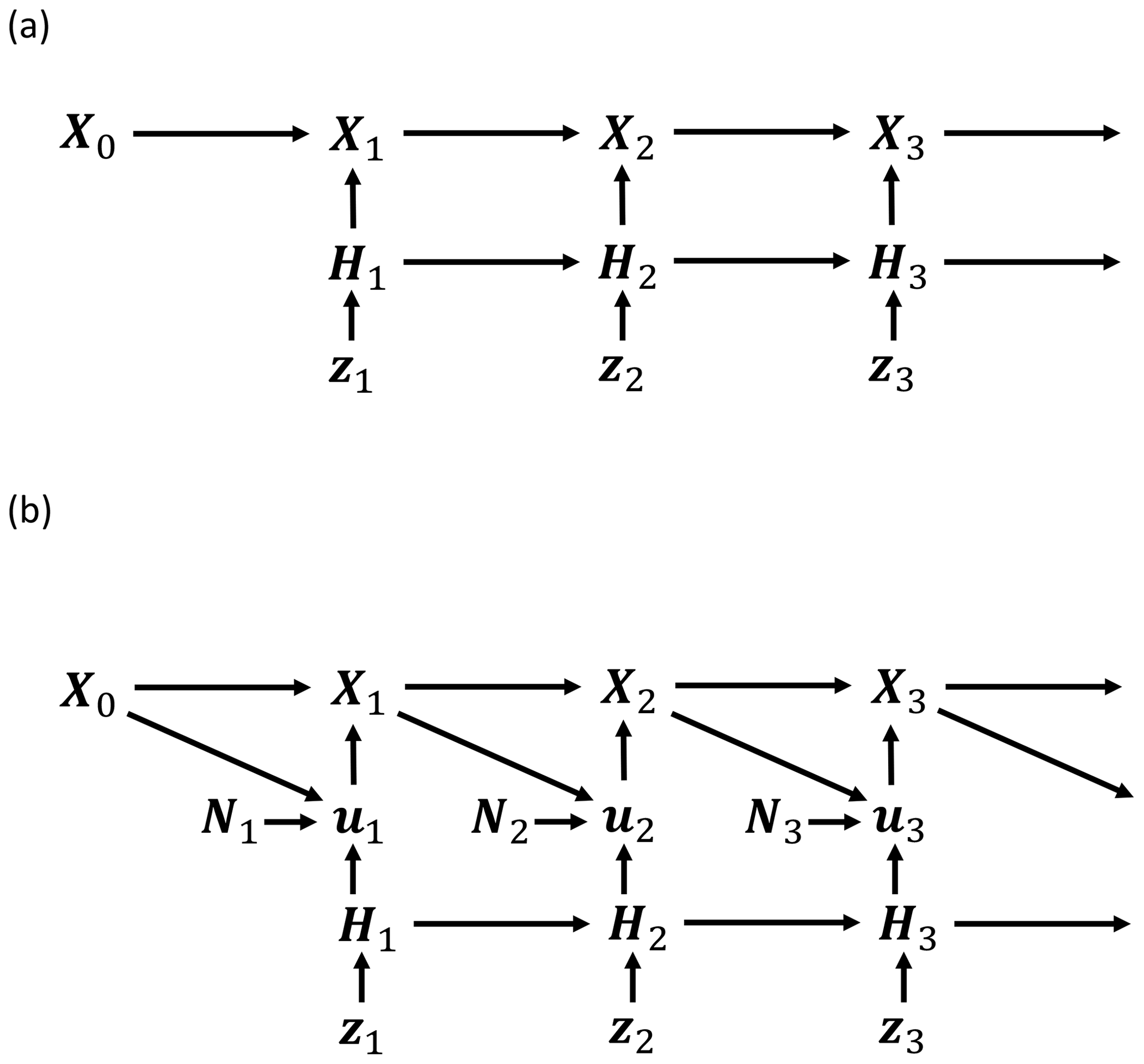
Figure 1 shows the mechanism of generation and the NN architectures used to learn the functions. The main architectural details are that s in Eq. (12) is implemented using two GRU layers, each composed of four units, and b in Eq. (11) is represented by a dense layer of size 1. g in Eq. (10) is implemented using three fully connected layers.

Here, as well as in the baselines, the parameterization models are “spatially local”, meaning that the full X_t vector is not taken in as input when modelling $X_{k,t+\mathrm{1}}$ anywhere apart from in ω_k(X_t). This is done to mimic parameterizations in operational weather and climate models. For all forecast models, Δt=0.005 model time units (MTU).

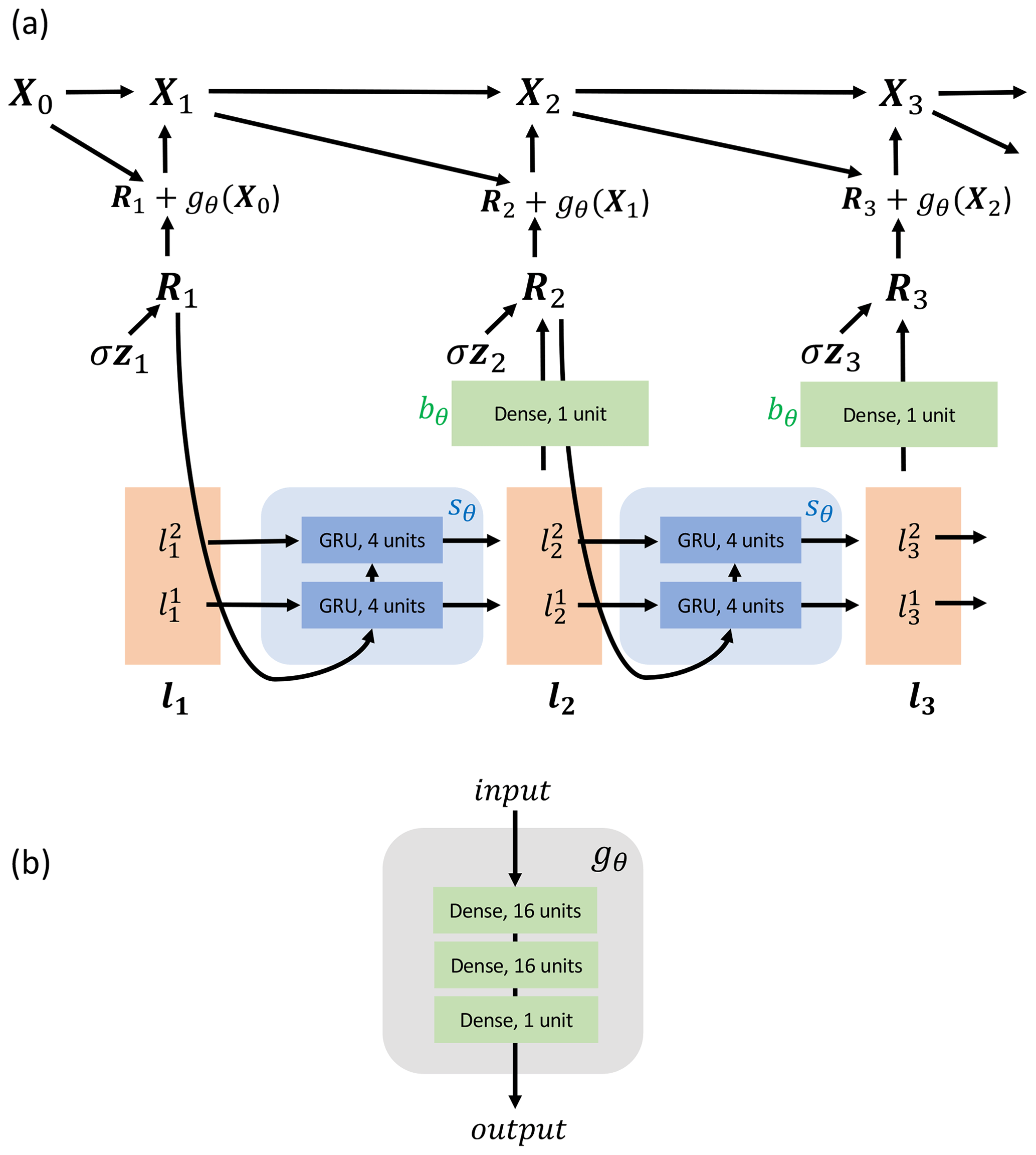
Figure 1 (a) RNN graphical model showing how each X_t is generated. X_t+1 is a function of X_t and R_t+1, and R_t is a function of l_t and z_t. z_t∈ℝ^K is the source of stochasticity. b_θ, s_θ and g_θ are NNs. l_t consists of a stack of $l_t^{\mathrm{1}}$ and $l_t^{\mathrm{2}}$, each ∈ℝ⁴. The neural networks are stacked K times (not shown in the figure), with each section of the stack being applied to each of the K components of X_t. (b) The architecture of the g_θ neural network.

3.2 Training probability models using likelihood

The L96-RNN is probabilistic and trained by maximizing the likelihood of sequences x_t in the training data, as is commonly done in the ML literature for RNN models (Bahdanau et al., 2014; Cho et al., 2014; Goodfellow et al., 2016; Sutskever et al., 2011, 2014). The “likelihood of a sequence” is denoted $\mathrm{Pr}(x_{\mathrm{1}},x_{\mathrm{2}},\mathrm{\dots },x_n)$ and can be interpreted as the probability assigned to a given sequence of variables $(x_{\mathrm{1}},x_{\mathrm{2}},\mathrm{\dots },x_n)$ by a given model. For our L96-RNN, the log likelihood (the natural logarithm of the likelihood) of a sequence of x_t is

$$\begin{array}{}\text{(13)}& \begin{array}{rl}& \log \mathrm{Pr}({\mathit{x}}_{\mathrm{1}},\mathrm{\dots },{\mathit{x}}_n;{\mathit{x}}_{\mathrm{0}})=\\ & \sum _{k=\mathrm{1}}^K\left(\log \mathrm{Pr}\right(r_{k,\mathrm{1}})+\sum _{t=\mathrm{2}}^n\log \mathrm{Pr}(r_{k,t}\left|l_{k,t}\right))\\ & -Kn\log \left(\mathrm{\Delta }t\right),\end{array}\end{array}$$

where the semicolon denotes that x₀ is given and r and l are deterministic functions of the training sequence ${\mathit{x}}_{\mathrm{0}},\mathrm{\dots },{\mathit{x}}_n$, derived from Eqs. (10)–(12). Specifically, by rearranging Eq. (10) we get

$$\begin{array}{}\text{(14)}& r_{k,t}={\displaystyle \frac{x_{k,t+\mathrm{1}}-x_{k,t}-{\mathit{\omega }}_k\left({\mathit{x}}_t\right)}{-\mathrm{\Delta }t}}-g_{\mathit{\theta }}\left(x_{k,t}\right),\end{array}$$

and so we can calculate what values r_k,t must take in order for the training sequence ${\mathit{x}}_{\mathrm{0}},\mathrm{\dots },{\mathit{x}}_n$ to be generated. Now, given the known sequence ${\mathit{r}}_{\mathrm{1}},\mathrm{\dots },{\mathit{r}}_n$ and the initial value l₁=0, the sequence of l values, ${\mathit{l}}_{\mathrm{1}},\mathrm{\dots },{\mathit{l}}_n$ can be calculated from Eq. (12). For example, $l_{k,\mathrm{3}}=s_{\mathit{\theta }}\left(s_{\mathit{\theta }}\right(l_{k,\mathrm{1}},r_{k,\mathrm{1}}),r_{k,\mathrm{2}})$. To reduce clutter in the final equation which we show in this section, we will rewrite Eq. (14) as

$$\begin{array}{}\text{(15)}& r_{k,t}=U_{k,t}-g_{\mathit{\theta }}\left(x_{k,t}\right),\end{array}$$

where $U_{k,t}=\frac{x_{k,t+\mathrm{1}}-x_{k,t}-{\mathit{\omega }}_k\left({\mathit{x}}_t\right)}{-\mathrm{\Delta }t}$ and can be understood as the true sub-grid forcing. Now, the explicit expression for the log likelihood is given by

$$\begin{array}{}\text{(16)}& \begin{array}{rl}& \log \mathrm{Pr}({\mathit{x}}_{\mathrm{1}},\mathrm{\dots },{\mathit{x}}_n;{\mathit{x}}_{\mathrm{0}})=\\ & \sum _{k=\mathrm{1}}^K(-\log (\mathit{\sigma }\sqrt{\mathrm{2}\mathit{\pi }})-{\displaystyle \frac{\mathrm{1}}{\mathrm{2}{\mathit{\sigma }}^{\mathrm{2}}}}(U_{k,\mathrm{0}}-g_{\mathit{\theta }}\left(x_{k,\mathrm{0}}\right){)}^{\mathrm{2}}\\ & +\sum _{t=\mathrm{2}}^n(-\log (\mathit{\sigma }\sqrt{\mathrm{2}\mathit{\pi }})-{\displaystyle \frac{\mathrm{1}}{\mathrm{2}{\mathit{\sigma }}^{\mathrm{2}}}}(U_{k,t}-g_{\mathit{\theta }}\left(x_{k,t}\right)-b_{\mathit{\theta }}\left(l_{k,t}\right){)}^{\mathrm{2}}\left)\right)\\ & -Kn\log \left(\mathrm{\Delta }t\right),\end{array}\end{array}$$

The L96-RNN is trained by maximizing this likelihood with respect to the parameters θ and σ. The explicit form of the L96-RNN likelihood makes training by maximum likelihood relatively straightforward. The full derivation of the likelihood is in Appendix A.

From Eq. (16) we can see that both the deterministic part (g_θ) and the stochastic model (b_θ and s_θ, which are involved via l_k,t) are trained jointly to minimize the mean squared error in the sub-grid forcing prediction. This is unlike the polynomial and GAN models where the deterministic part is fitted first and then the stochastic part is modelled in a separate step.

3.3 RNN training

Truth data for training were created by running the full L96 model five separate times with the following values of F: $(\mathrm{19},\mathrm{20},\mathrm{20.5},\mathrm{21},\mathrm{21.5})$. Henceforth, we use truth data to refer to data from the full L96 model. We gave our model data from different forcing scenarios so it could learn how perturbations in the forcing may affect the evolution of X_t. The GAN and polynomial were trained in a similar manner to allow for a fair comparison. The truth data were created by solving the two-level L96 equations using a fourth-order Runge–Kutta time stepping scheme and a fixed time step Δt=0.001 MTU, with the output saved at every 0.005 MTU. A training set of the length 2500 MTU was assembled from the truth data, consisting of three equal 500 MTU components with $F=(\mathrm{19},\mathrm{20.5},\mathrm{21})$ and one 1000 MTU component with F=20, with a F=21.5 set of the length 500 MTU kept as a validation hold-out set. This resulted in a 75:25 training : validation set split (3 999 992 samples : 800 008 samples).

The L96-RNN was trained using truncated back propagation through time on sequences of a length of 700 time steps for 100 epochs with a batch size of 32 using Adam (Kingma and Ba, 2014), with θ and σ being the learnable parameters. A variable learning rate was used, starting at 0.0001 for the first 70 epochs and decayed to 0.00003 for the remaining 30. A small grid search was conducted over the number of GRU layers (searching over 1 to 3) and the GRU unit sizes (searching between 4 to 16). The model parameters which gave the lowest loss on the validation set were saved.

4 Results

This section analyses performance across a range of timescales. The first results are for F=20. Assessing the model in the training realm allows us to verify if it can replicate the L96 attractor. Later experiments are for F≥28. For F=20 and F=28, 50 000 MTU long simulations (≈685 “atmospheric years”) were created for analysis.

4.1 Weather evaluation

The models were evaluated in a weather forecast framework. A total of 745 initial conditions were randomly taken from the truth data, and an ensemble of 40 forecasts each lasting 3.5 MTU were generated from each initial condition. Figure 2 shows the spread and error terms for these experiments over time. The error is defined as

$$\text{error}\left(t\right)=\sqrt{{\displaystyle \frac{\mathrm{1}}{M}}\sum _{m=\mathrm{1}}^M\left(X_m^{\mathrm{O}}\right(t)-\stackrel{\mathrm{‾}}{X_m^{\text{sample}}\left(t\right)}{)}^{\mathrm{2}}},$$

where there are M different initial conditions, $X_m^{\mathrm{O}}\left(t\right)$ is the observed state at time t for the mth initial condition and $\stackrel{\mathrm{‾}}{X_m^{\text{sample}}\left(t\right)}$ is the ensemble mean forecast at time t.

The spread is defined as

$$\text{spread}\left(t\right)=\sqrt{{\displaystyle \frac{\mathrm{1}}{M}}\sum _{m=\mathrm{1}}^M{\displaystyle \frac{\mathrm{1}}{N}}\sum _{n=\mathrm{1}}^N\left(X_{m,n}^{\text{sample}}\right(t)-\stackrel{\mathrm{‾}}{X_m^{\text{sample}}\left(t\right)}{)}^{\mathrm{2}}},$$

where N is the number of ensemble members and $X_{m,n}^{\text{sample}}\left(t\right)$ is the state of the nth member at time t for the mth initial condition.

As noted by Leutbecher and Palmer (2008), for a perfectly reliable forecast (defined as one where $X_{m,n}^{\text{sample}}\left(t\right)$ and $X_m^{\mathrm{O}}\left(t\right)$ are independent samples from the same distribution), for large N and M the error should be equal to the spread. A smaller error implies an ensemble forecast that better matches observations, and a spread / error ratio close to 1 implies a reliable forecast. Figure 2 shows that the polynomial and the L96-RNN have the smallest errors, but the L96-RNN has the better spread / error ratio until 1.0 MTU. After that, its spread is still slightly better matched to its error compared to the polynomial. The GAN is underdispersive, with the greatest error but smallest spread / error ratio, suggesting it is overconfident in its predictions.

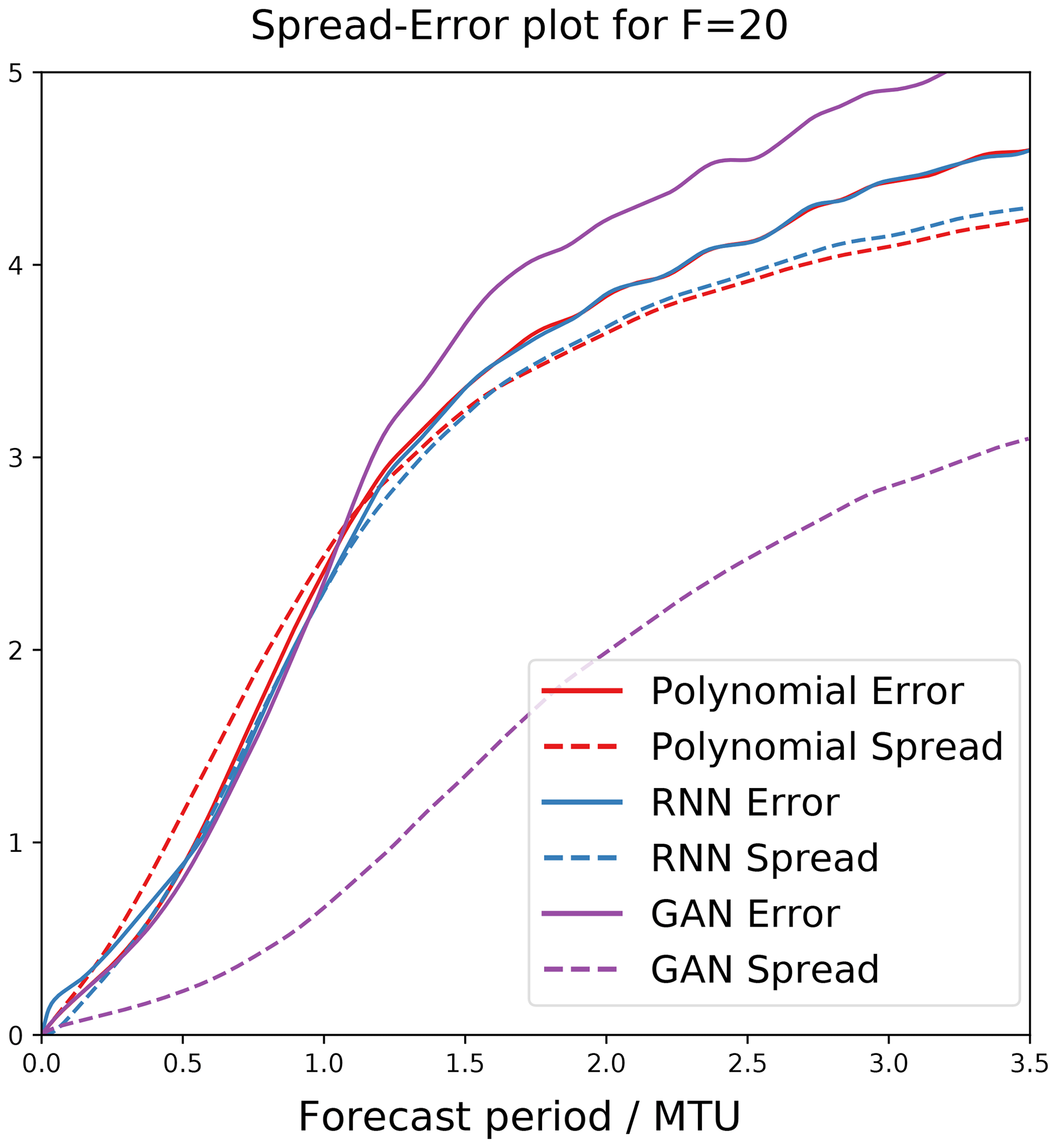
Figure 2 Error and spread for weather experiments. We expect a smaller error for a more accurate forecast model. The spread / error ratio would be close to 1 in a “perfectly reliable” forecast.

4.2 Climate evaluation

The ability to simulate the climate of the L96 was evaluated using the 50 000 MTU simulations. We use histograms to represent various climate-related distributions. For example, Fig. 3a represents each model's marginal distribution of X_k,t. Since the true continuous distributions for this quantity are unavailable, we represent them using histograms (a discrete estimate). The idea of estimating an underlying continuous distribution's density with a discrete distribution based on a finite set of sampled points is commonplace and known as histogram density estimation (Silverman, 1986; Wilks, 2011). When plotting histograms, an appropriate bin width is necessary. Too few bins will lead to over-smoothing where the underlying distribution's shape is not captured, whilst too many bins will lead to under-smoothing. Both cases lead to poor representations of the underlying distribution. We use the Freedman–Diaconis rule (Freedman and Diaconis, 1981) to determine the bin widths (and therefore number of bins). The rule is based on minimizing the mean integrated squared error between the histogram's density estimate and the true density function. The number of bins used are noted in the relevant figure captions.

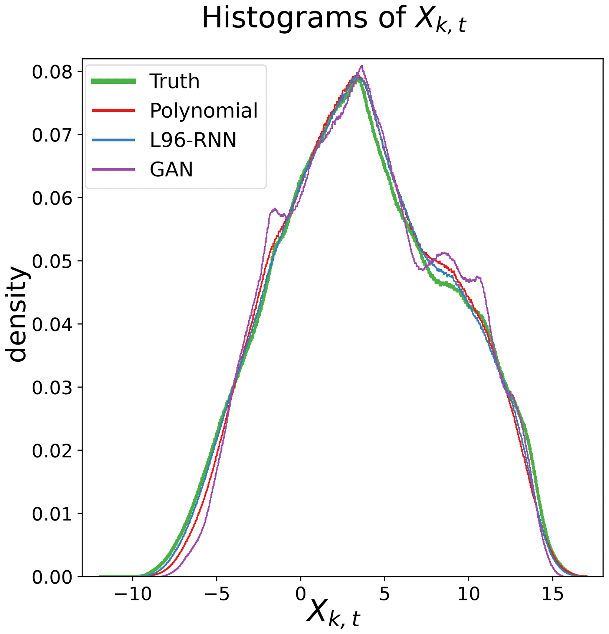
Figure 3 Histograms of X_k,t. The truth histogram is shown in green and bold. The closer a model's histogram to the truth, the better it models the probability density of X_k,t. A total of 827 bins are used for all shown models.

We can quantitatively measure how well the histogram density estimates from each model match the histogram density estimate from the truth using KL (Kullback–Leibler divergence) divergence. The KL divergence has a direct equivalence to log likelihood: minimizing the KL divergence between a true distribution and a model's distribution is equivalent to maximizing the log likelihood of the true data under the model. We evaluate the KL divergence between q(a), the distribution described by the histogram of a variable A in the true L96 model, and p(a), the distribution described by the histogram of that variable in a parameterized model, using

$$\text{KL}\left(q\right(a\left)\right|\left|p\right(a\left)\right)=\sum _{a}q\left(a\right)\log {\displaystyle \frac{q\left(a\right)}{p\left(a\right)}},$$

where the sum is over all the discrete values which A takes. The smaller this measure, the better the goodness of fit. The calculated KL divergence is obviously dependent on the number of bins used in our histograms. Using a number of bins=1 would give a KL divergence of 0, whilst using a number of bins=n, where n is the number of data points, would give a KL divergence of ∞ in this case as the variables under consideration are continuous so their empirical probability density functions will not overlap. Therefore, a bin number which best represents the underlying distribution is important to use. As noted earlier, we use the Freedman–Diaconis rule for this. Nevertheless, we also provide results in Appendix B for the KL divergences for a range of bin numbers centred on the Freedman–Diaconis suggestions.

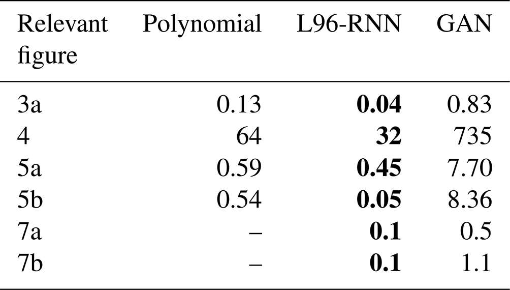
Successful reproduction of the L96 climate would result in a model's histogram matching the truth model's. Qualitatively, from Fig. 3, the polynomial and the L96-RNN are closest to the truth, with the L96-RNN doing slightly better around $X_{k,t}=\mathrm{9}$. Quantitatively, the KL divergence results (Table 1) confirm that the L96-RNN best matches the truth model here. Results from Appendix B confirm that the stronger L96-RNN performance is also seen over a range of bin numbers.

Table 1 KL divergence (goodness of fit) between (1) the truth and (2) the parameterized models, for the distributions shown in the noted figures. The smaller the KL divergence, the better the match between the true and modelled distributions. The best model in each case is shown in bold.

The L96 model used here displays two distinct regimes with separate dynamics. We use the approach from Christensen et al. (2015) to examine the regimes. First, the time series are temporally smoothed with a running average over 0.4 MTU to help identify regimes (Stephenson et al., 2004; Straus et al., 2007). The dimensionality of the system is then reduced using principal component analysis, as is often done when studying atmospheric data (Selten and Branstator, 2004; Straus et al., 2007). For the truth time series, the components PC1 (principal component 1) and PC2 (principal component 2) are degenerate, offset in phase by $\mathit{\pi }/\mathrm{2}$ radians, and represent wavenumber 2 oscillations. PC3 and PC4 are also degenerate, offset in phase by $\mathit{\pi }/\mathrm{2}$ radians, and represent wavenumber 1 oscillations. All model runs are projected onto the truth model's components. Given the degeneracies, the magnitudes of the principal component vectors, $\left|\right|$[PC1, PC2]$\left|\right|$ and $\left|\right|$[PC3, PC4]$\left|\right|$, where $\left|\right|$[PC1, PC2]$\left|\right|=\sqrt{\mathrm{PC}{\mathrm{1}}^{\mathrm{2}}+\mathrm{PC}{\mathrm{2}}^{\mathrm{2}}}$, are computed and histograms of the system are plotted in this space.

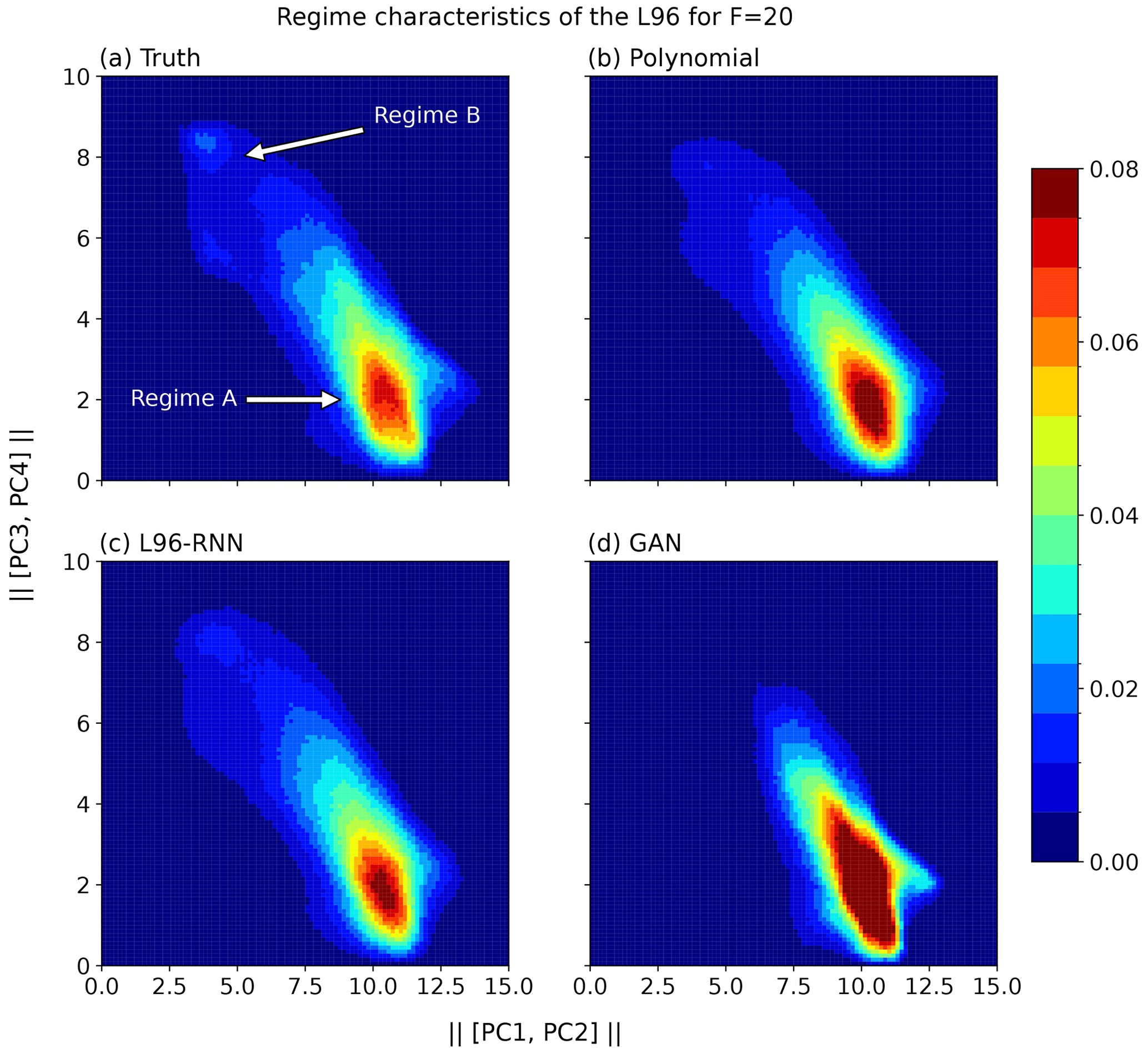
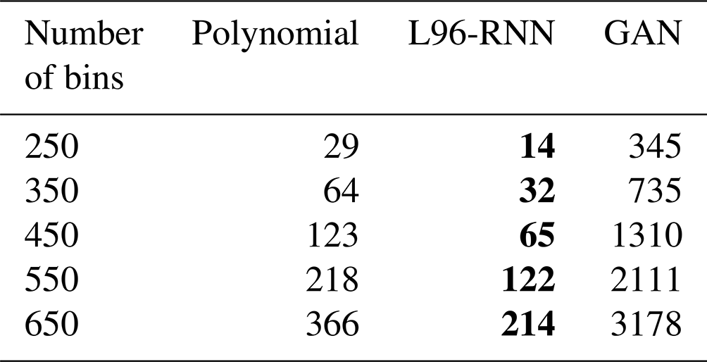
Figure 4 Regime characteristics of the L96 for F=20. Two-dimensional histograms show the magnitudes of the projections of X_k,t onto the principle components from the truth series. A total of 100 bins are used for this visualization. When calculating the KL divergence in Table 1, 350 bins are used.

The presence of two regimes is apparent in Fig. 4a where there is a large maximum corresponding to the major regime, A, but also a smaller peak corresponding to the minor regime, B. The polynomial and GAN fail to capture the two regimes, whereas the L96-RNN is more successful. Comparison is made easier by decomposing the 2D Fig. 4 into two 1D density plots (Fig. 5). We can use the KL divergence to measure how well our models match the truth across all three histograms. Table 1 shows that the L96-RNN best matches the truth and so captures the regime characteristics best. There are still evidently deficiencies though as further density is required to be placed around Regime B.

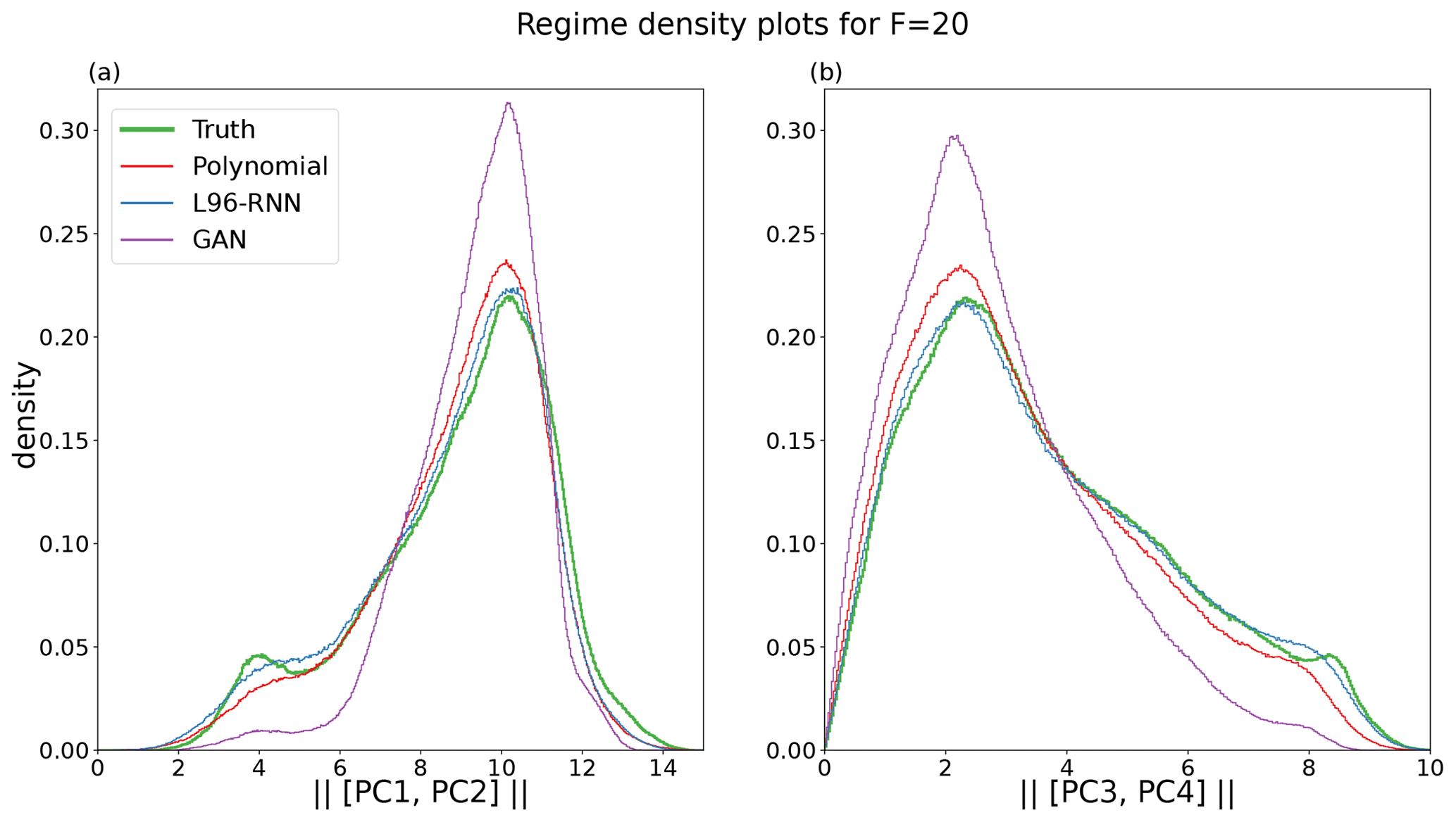
Figure 5 Density plots for each regime for F=20. The truth is shown in green and bold. (a) Magnitude of [PC1, PC2]. A total of 534 bins are used for this. (b) Magnitude of [PC3, PC4]. A total of 350 bins are used for this.

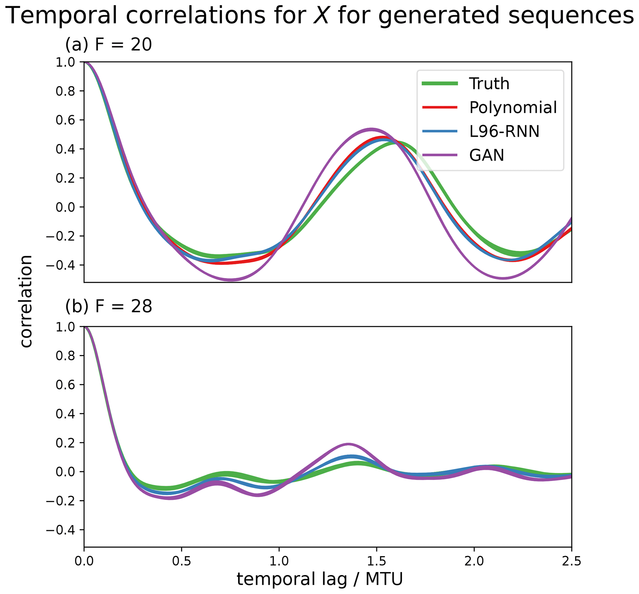
Figure 6 The ability of the parameterized models to reproduce the “true” temporal correlations of the X variables in the L96 system (green). The correlations for each of the K components are plotted – the variability is indicated by the line width. Panel (a) is for the sequences generated with F=20, and (b) is for those with F=28. The polynomial is not shown for (b) as the simulations are unstable and go to infinity.

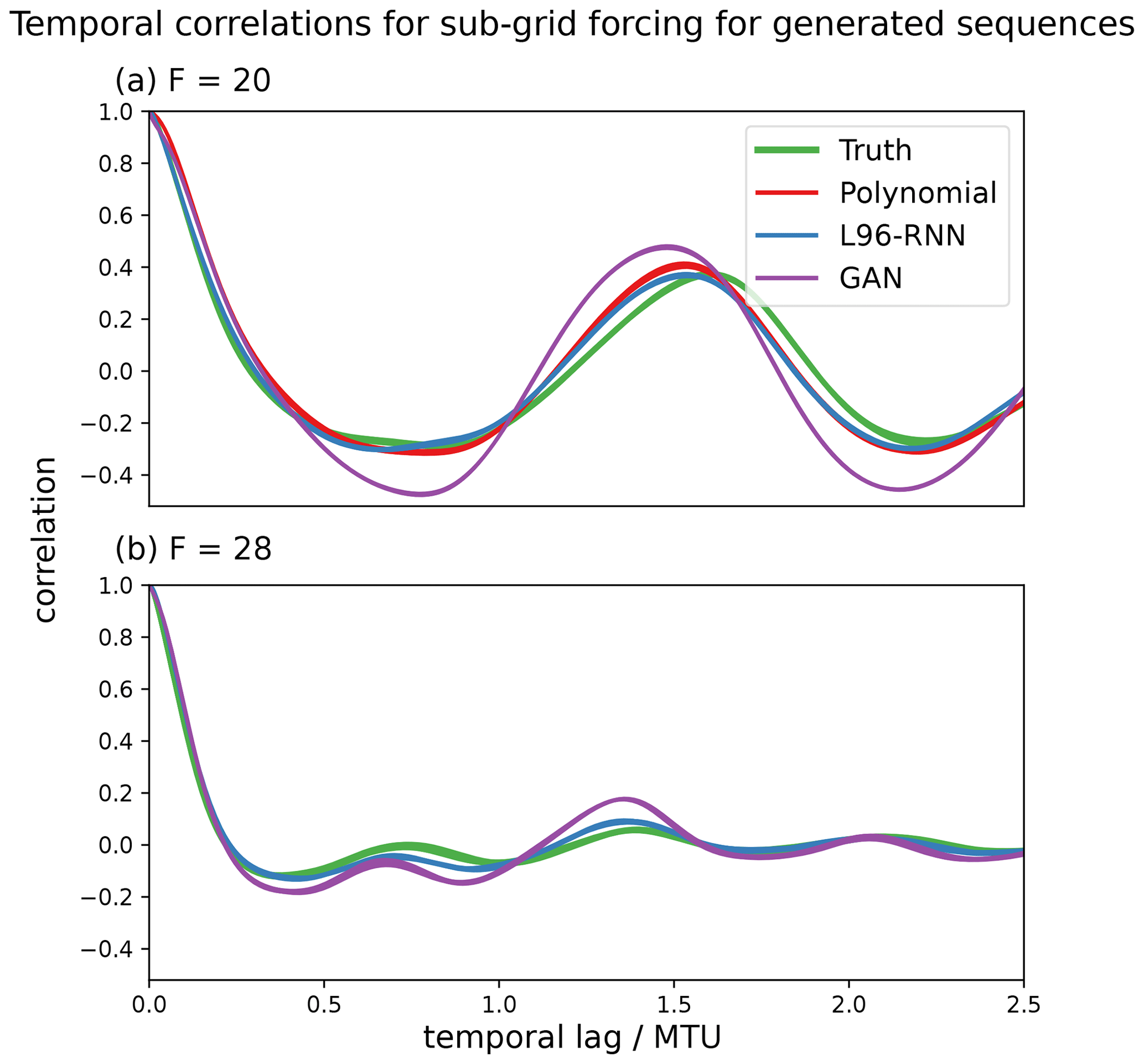
Figure 7 The ability of the parameterized models to reproduce the “true” temporal correlations of the sub-grid forcing terms (U) in the L96 system (green). The correlations for each of the K components are plotted – the variability is indicated by the line width. Panel (a) is for the sequences generated with F=20, and (b) is for those with F=28. The polynomial is not shown for (b) as the simulations are unstable and go to infinity.

We desire our parameterized models to correctly capture the temporal behaviour of the L96 system. One way to assess this is by considering the temporal correlations (linear associations) using an autocorrelation plot. The autocorrelation plots of the generated X variables are shown in Fig. 6, and those of the corresponding sub-grid forcing terms, U, are shown in Fig. 7, where $U_{k,t}=\frac{x_{k,t+\mathrm{1}}-x_{k,t}-{\mathit{\omega }}_k\left({\mathit{x}}_t\right)}{-\mathrm{\Delta }t}$. In Fig. 6a we see that for F=20, all the parameterized models perform well, but the L96-RNN best captures the trough behaviour at the 0.7 temporal lag. In Fig. 7a, for F = 20, the L96-RNN and polynomial perform the best.

4.3 Generalization experiments

We set the L96 forcing to $F=\mathrm{28},\mathrm{32},\mathrm{35}$, and 40 and examine how the models can capture changes due to varying external forcings. These F values are notably different to those in the training data and so allow us to test generalization. For example, the change from F=21.5 (validation set) to F=28 results in the following changes to the regime structure: the centroid location of the rarer regime shifts to higher values of $\left|\right|\left[\text{PC1, PC2}\right]\left|\right|$ and $\left|\right|\left[\text{PC3, PC4}\right]\left|\right|$ (Fig. 8), and the proportion of time spent in the rarer regime increases from 38 % to 50 %. The range of X_k,t also increases from $[-\mathrm{12},\mathrm{19}]$ to $[-\mathrm{24},\mathrm{29}]$. The differences in wave behaviour between regimes means the above changes result in different system dynamics.

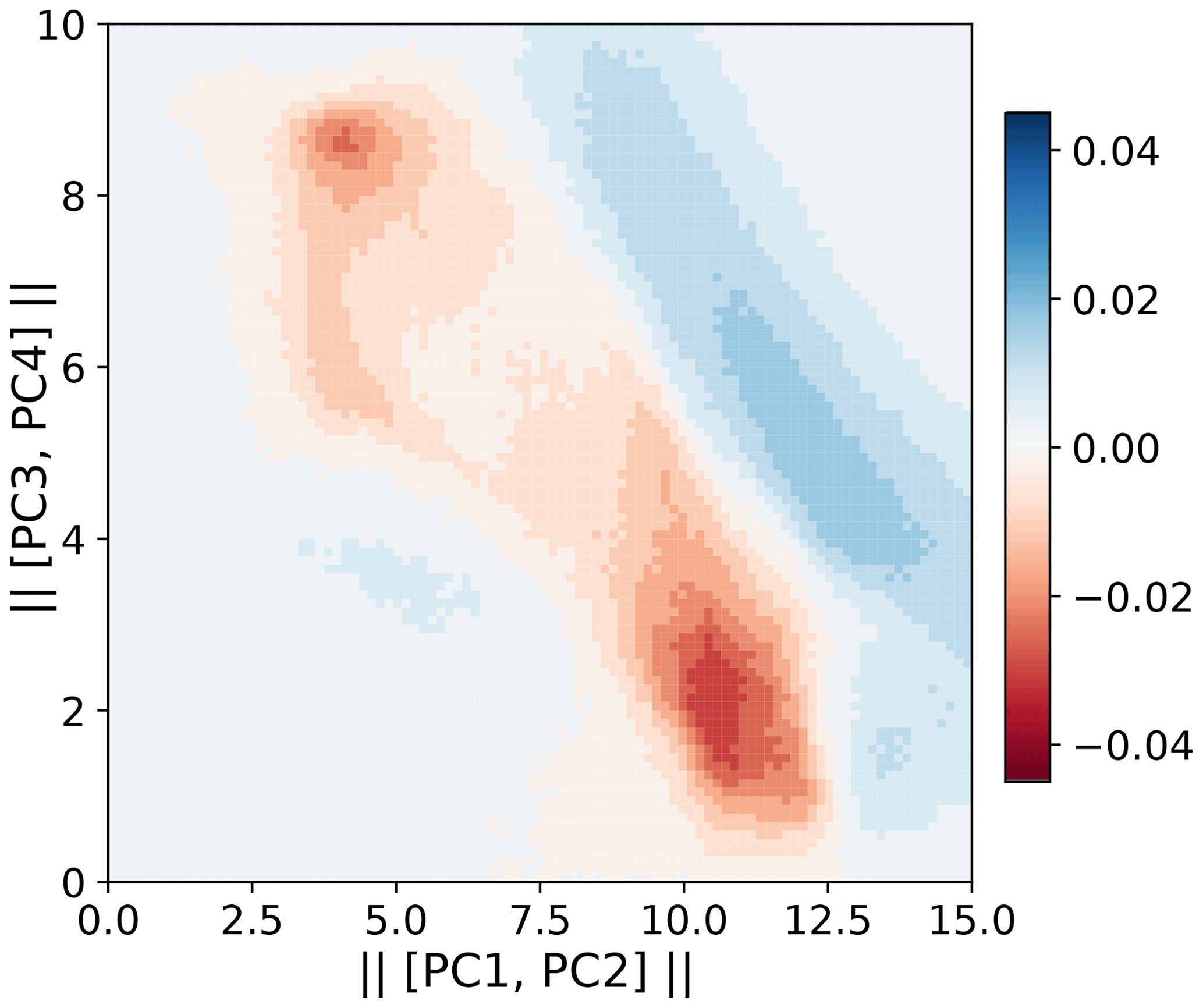
Figure 8 Difference between the F=21.5 and F=28 densities in principal component space. The principal components are those from the F=20 truth series. A total of 100 bins are used for this visualization.

In all the below experiments the polynomial model's trajectories exploded (went to infinite values), so the polynomial is omitted. This is merely due to the specification of a third-order polynomial. It significantly deviates from its target values when X_k,t values notably different from those in training (such as $X_{k,t}\ge \mathrm{19}$) are taken as inputs.

The F=28 climate was explored in a similar manner to the F=20 one. First, for the histograms of X_k,t (analogous to Fig. 3) the L96-RNN and GAN both had small KL divergences (0.02 vs. 0.14). Next, the principal component projections were examined (analogously to Fig. 4). The same components as determined from the F=20 truth data set are used. In this space, the L96-RNN has a smaller KL divergence (11) than the GAN (57). Figures for the above two plots are omitted due to it being hard to visually distinguish between the models. As before, further comparison can be made by examining the two, 1D density plots in Fig. 9 (analogously to Fig. 5). Both models perform well (KL divergence in Table 1), but neither put enough density in the right-hand side tails. In terms of temporal correlation, as seen in Figs. 6b and 7b, both models perform well, but the L96-RNN generally tracks the periodicity and the amplitude of the peaks and troughs better.

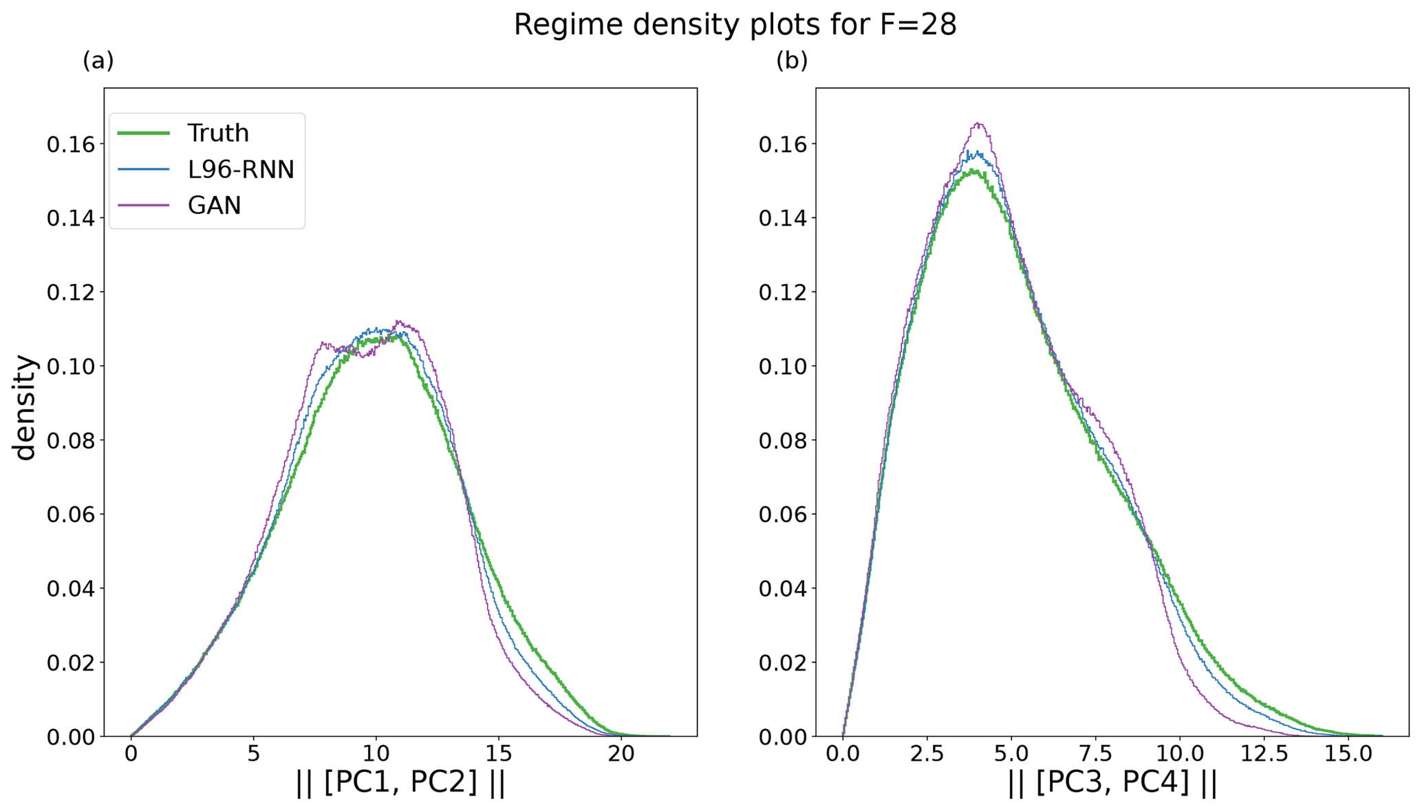
Figure 9 Density plots for each regime for F=28. The truth is shown in green and bold. (a) Magnitude of [PC1, PC2]. A total of 479 bins are used. (b) Magnitude of [PC3, PC4]. A total of 444 bins are used. The right-hand side tails are not given sufficient density by the L96-RNN or the GAN.

The models were also evaluated in the weather forecasting framework for $F=\mathrm{28},\mathrm{32},\mathrm{35}$, and 40. A total of 750 initial conditions were randomly selected from the truth attractors, and an ensemble of 40 forecasts each lasting 2.5 MTU were produced. Figure 10 shows the L96-RNN generally has lower errors than the GAN, with a better matching spread. The GAN continues to be underdispersive.

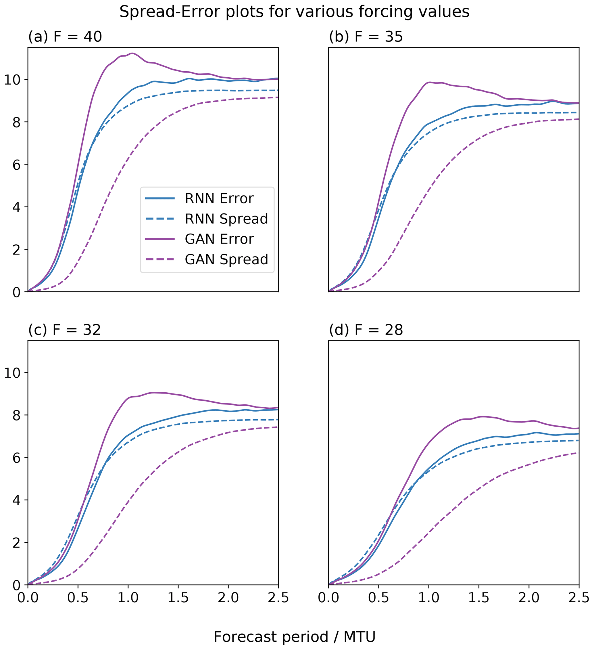
Figure 10 Error and spread for weather experiments for varying forcing values. This is done to assess generalization performance. The L96-RNN's spread is best matched to its error, unlike the GAN.

4.4 Residual analysis

We can also compare the polynomial and the L96-RNN's ability to capture temporal patterns by assessing their residuals. The residuals are the differences between observed data and a model's predictions. It can be considered an offline metric. For the proposed models, the residuals should be uncorrelated and resemble white noise. In Fig. 11 we show the autocorrelation of the residuals. Ideally, there would be no significant autocorrelation. Neither of the models succeeds in this aspect, but the autocorrelation of the L96-RNN's residuals drops off far quicker than that of the polynomial. This is likely due to the L96-RNN's ability to capture longer temporal trends. The L96-RNN still has a decaying oscillation, suggesting further changes must be made to the model to account for this.

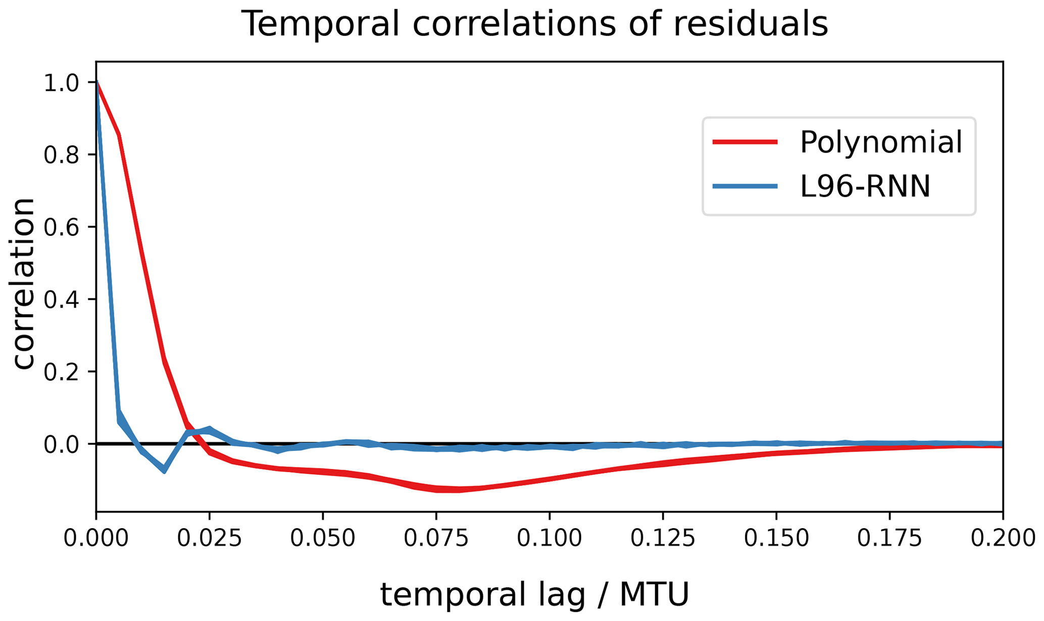
Figure 11 Autocorrelation plot of the residuals for the polynomial and the L96-RNN. Ideally, these would show no correlations (and match the black line). The L96-RNN's residual correlations decay more quickly than the polynomial's.

4.5 Computational costs

We wish our models to have a lower simulation cost than the full L96. This is measured by considering the number of floating-point operations per simulated time step (Δt=0.005). The L96-RNN (8682) is notably cheaper than the truth model (88 000) and the GAN (14 074) and so meets the computational cost objective of parameterization work. The polynomial (334) is the cheapest.

In terms of training times, both ML models were trained using a 32 GB NVIDIA V100S GPU. The L96-RNN and GAN took 12 min and 30 h respectively.

5 Evaluation and diagnostics using likelihood

5.1 Hold-out likelihood

We also evaluate using the likelihood (explained in Sect. 3.2) of hold-out data. This is a standard approach in the ML literature. Evaluation is done on hold-out sets to ensure that overly complex models which just overfit the training data are not selected.

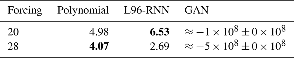
Here, hold-out sets for F=20 and F=28 were created by taking a 10 000 MTU subset from the 50 000 MTU truth sets created in Sect. 4. The hold-out log likelihoods are shown in Table 2. The likelihood for the polynomial model and its derivation is in Appendix A. We also present an approach to approximate the GAN likelihood. This is despite its full form being intractable (involving integrals which cannot be efficiently approximated using Monte Carlo sampling), meaning it is not typically used to evaluate GANs. This is also detailed in Appendix A. The L96-RNN has a worse likelihood on F=28 than the polynomial, despite the polynomial simulations exploding, unlike the L96-RNN's. This is discussed below.

5.2 What is the use of likelihood?

5.2.1 For evaluation

The other metrics used above only capture snapshots of model performance. Likelihood is a composite measure which assesses a model's full joint distribution (Casella and Berger, 2002). For example, in the univariate case, the mean squared error and variance of a model show two separate things about its performance, with implicit assumptions being made about variables being normally distributed (as is the case whenever mean squared error is used). The likelihood captures both of these and without enforcing such assumptions.

Likelihood also captures information about more complex, joint distributions, saving the need for custom metrics to be invented to assess specific features. To illustrate this, consider that we wish to assess a model's temporal associations (not just the linear temporal correlations). The likelihood already contains this information. Although custom metrics could be invented to assess this, the likelihood is an off-the-shelf metric which is already available. We suggest it is wasteful not to use it.

Using a composite metric brings challenges though. Poor performance in certain aspects may be overshadowed by good performance elsewhere. This can result in cases where increased hold-out likelihoods do not correspond to better sample quality, as noted in the ML literature (Goodfellow et al., 2014; Grover et al., 2018; Theis et al., 2015; Zhao et al., 2020) and seen in our results: the L96-RNN has a worse F=28 hold-out likelihood than the polynomial (Table 2), yet the polynomial model explodes unlike the L96-RNN. In this case, the phenomenon of “explosion” does not significantly penalize the likelihood. This links to how likelihood is evaluated on trajectories of the true system, so is an “offline” metric. Just as with the offline metric of mean squared error, you would expect better “online” performance (the performance of generated simulations) as the likelihood improves, but there is no guarantee of a monotonic relationship between the two. Likelihood is therefore a complement to, not a replacement of, to other metrics which are important to the end user.

5.2.2 For diagnostics

Likelihood's composite nature makes it a helpful diagnostic tool. Just like KL divergence, the further away a model is – in any manner – from the data in the hold-out set, the worse the likelihood will be. If a model has a poor likelihood despite performing well on a range of standard metrics, this suggests there are still deficiencies in the model which need investigating. For example, with the L96-RNN at F=28, the poor average likelihood (Table 2) is caused by a tiny number of segments of the X_k,t sequences being extremely poorly modelled (and therefore having extremely poor likelihoods assigned). On inspection, the issue is due to the choice of a fixed σ in Eq. (11) – this is appropriate for most of the time series, but for parts which are difficult to model, it is too small, preventing the model from expressing sufficient uncertainty. This could be rectified by allowing σ to vary, and we suggest future work explore this.

Table 2 Log likelihood on hold-out data for different forcing values. The best model in each case is shown in bold.

6 Discussion and conclusion

We present an approach to replace red noise with a more flexible stochastic machine-learnt model for temporal patterns. Even though we used ML to model the deterministic part g_θ(X_k,t) in Eq. (10), the real benefit came from using ML to model the hidden variables. For example, on setting g_θ(X_k,t) in our model equal to $a{X}_{k,t}^{\mathrm{3}}+b{X}_{k,t}^{\mathrm{2}}+c{X}_{k,t}+d$ from the polynomial baseline, our model performance hardly suffered (and the cost halved) for F=20. This finding is supportive of physics-based ML approaches where conventional parameterizations are augmented with a stochastic term learnt using ML.

Using physical knowledge to structure ML models can help with learning. The L96-RNN includes “physically relevant” features for the L96, particularly advection, in Eq. (10). This gave better results than when we modelled the system without them (e.g. when we used an RNN to do the full updating step of X_t given ${\mathit{X}}_{t-\mathrm{1}},\mathrm{\dots },{\mathit{X}}_{\mathrm{0}}$). Although in theory a NN can learn to create helpful features (such as advection), giving these useful features can make learning easier. The NN does not need to learn the known, useful physical relationships and instead can focus on learning other helpful ones.

There are more sophisticated models which can be used for the L96 system. We noticed that in some cases the L96-RNN struggled even to overfit the training data, regardless of the L96-RNN complexity. This could be due to difficulties in learning the evolution of the hidden variables. Creating architectures that permit better hidden variables to be learnt (ones which model long-term correlations better) would give better models. Despite our use of GRU cells, which along with the LSTM were great achievements in sequence modelling, we still faced issues with the modelling of long-term trends as evidenced in Fig. 11. Attention-based models such as the Transformer (Vaswani et al., 2017) may improve on this. Separately, certain models (mainly those which did not leverage physical structure) resulted in unstable simulations. Using hierarchical models which learn to model trends at different temporal resolutions (Chung et al., 2016; Liu et al., 2020) may provide improvement. Our particular model had specific limitations on how the hidden state, R_t, was not a function of X_t−1, unlike the GAN, and on how σ was not a function of other variables. We did this to make a clearer comparison between hidden variables modelled with AR1 processes versus those modelled with RNNs. Nevertheless, it is simple to include X_t−1 in the model for R_t and to make σ a neural network function of other variables (including the forcing) if desired. We believe the latter change would be particularly useful in better capturing uncertainty.

We trained the L96-RNN using the likelihood of the sequence $({\mathit{x}}_{\mathrm{0}},{\mathit{x}}_{\mathrm{1}},\mathrm{\dots },{\mathit{x}}_n)$ and showed how, for an RNN-based model, there is an explicit form of the likelihood which makes likelihood calculations tractable. In the L96, these X_t sequences are K-dimensional and correlated. Their likelihood can be written in terms of the likelihood of the hidden variables $({\mathit{r}}_{\mathrm{1}},{\mathit{r}}_{\mathrm{2}},\mathrm{\dots },{\mathit{r}}_n)$, and as shown in Eq. (13), training to maximize the likelihood of a sequence of hidden variables is equivalent to maximizing the likelihood of an X_t sequence. However, in the general case of a general circulation model, it will often not be possible to analytically derive the relationship between the likelihood of an X_t sequence and that for a sequence of hidden variables, as explained in Sect. A4.1. Therefore, maximizing the likelihood of other variables (the approach typically taken), such as the hidden variables or sub-grid terms, may not correspond to maximizing the likelihood of X_t. This is unideal as our actual goal is to create a model which generates realistic sequences of X_t. And this may be a reason why online evaluations of such models often show error accumulation leading to simulation blow-ups (Brenowitz and Bretherton, 2018; Rasp, 2020). In future work, we plan to investigate how to better train parameterization models for cases where you cannot easily maximize a likelihood which is proportional to the likelihood of X_t.

Learning from all the high-resolution data whilst still being computationally efficient at simulation time is an interesting idea. Whilst we cannot keep all the high-resolution variables in our schemes (as otherwise we might as well run the high-resolution model outright – which is not possible as it is too slow for the desired timescales and is a reason why this field of work exists), only keeping the average (as in existing work which coarse-grains data) means many data are thrown away. Our preliminary investigations used the graphical model in Fig. 12. We designed this so that in training, l_t is learnt such that it contains useful information about the high-resolution data, Y_t, whereas during generation, Y_t is not required to be simulated. For the L96, this showed no improvement over our L96-RNN though. Parthipan and Wischik (2022) show that such an approach may be useful as a regularizer when training data are limited.

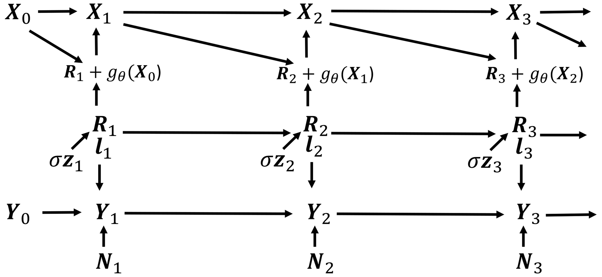
Figure 12 Model which allows learning from high-resolution data without requiring it at simulation time, where $N_t\sim \mathcal{N}(\mathrm{0},I)$. The model is trained to generate Y and so learns from these data, but at simulation time, Y is not required to generate X.

Further work with GANs could result in better models. There may be aspects of realism which we either may not be aware of or may not be able to quantify, so they are difficult to include explicitly in our probability models. The GAN discriminator could learn what features constitute “realism” and so the generator may learn to create sequences which contain these. However, we found that using the adversarial approaches from GANs and Wasserstein GANs (Arjovsky et al., 2017; Gulrajani et al., 2017) to train the L96-RNN (instead of by likelihood) did not show any benefit. This may be due to the difficulty of training GANs on longer sequences. They have been used to train RNNs on medical time series (Esteban et al., 2017) and to model music (Mogren, 2016), so applying this approach to climatic sequences may be something for future work to reconcile. The challenges of using GANs are seen by how we have not been able to reproduce the results shown in Gagne et al. (2020) despite the same set-up. This points to the instability of GAN training, as noted by them too. Mode collapse is a common issue encountered when training GANs, where the generator fails to produce samples that explore certain modes of the distribution, and could explain why density is only present for Regime A in Fig. 4 and not for Regime B.

7 Conclusions

We have shown how to build on the benefits of red-noise models (such as AR1 ones) in parameterizations by using a probabilistic ML approach based on a recurrent neural network (RNN). This can be seen as a natural generalization of the classical autoregressive approaches. This is done in the idealized case of the two-level Lorenz 96 system, where the unresolved variables must be parameterized. Our L96-RNN outperforms the red-noise baselines (a polynomial model and a GAN) in a weather forecasting framework and has lower KL divergence scores for the probability density functions arising from long-range simulations. The L96-RNN generalizes the best to new forcing scenarios. These strong empirical results, along with a less correlated residual pattern, supports the benefit of the L96-RNN being due to it better capturing temporal patterns.

This approach now needs testing on more complex systems – both to specifically improve on AR1 processes and to learn new, more flexible models of X_t. An interesting area for further work is to examine what information is tracked in the hidden variables of the L96-RNN and how this relates to the timescales of the required memory in the modelled system. The field is ripe for other probabilistic ML tools to be used, and we suspect that further customization of these will lead to many improved parameterization models.

Likelihood can often be fairly easily calculated, and where this is the case, we propose that the community also evaluate the hold-out likelihood for any devised probabilistic model (ML or otherwise). It is a useful debugging tool, assessing the full joint distribution of a model. It would also provide a consistent evaluation metric across the literature. Given the challenges relating to sample quality, likelihood should complement, not replace, existing metrics.

Finally, we have used demanding tests to show that ML models can generalize to unseen scenarios. We cannot hope for ML models to generalize to all settings. We do not expect this from our physics-based models either. But ML models can generalize outside their training realm. And it is by using challenging hold-out tests that we can assess their ability to do so and, if they fail, begin the diagnosis of why.

Appendix A: Likelihood derivations

In all cases, the log likelihood of the sequence of X_t is given by

$$\begin{array}{}\text{(A1)}& \begin{array}{rl}& \log \mathrm{Pr}({\mathit{x}}_{\mathrm{1}},\mathrm{\dots },{\mathit{x}}_n;{\mathit{x}}_{\mathrm{0}})=\log \mathrm{Pr}({\mathit{x}}_{\mathrm{1}};{\mathit{x}}_{\mathrm{0}})\\ & +\log \mathrm{Pr}\left({\mathit{x}}_{\mathrm{2}}\right|{\mathit{x}}_{\mathrm{1}};{\mathit{x}}_{\mathrm{0}})+\log \mathrm{Pr}({\mathit{x}}_{\mathrm{3}}|{\mathit{x}}_{\mathrm{2}},{\mathit{x}}_{\mathrm{1}};{\mathit{x}}_{\mathrm{0}})\\ & +\mathrm{\dots }+\log \mathrm{Pr}\left({\mathit{x}}_n\right|{\mathit{x}}_{n-\mathrm{1}},\mathrm{\dots },{\mathit{x}}_{\mathrm{1}};{\mathit{x}}_{\mathrm{0}}),\end{array}\end{array}$$

which follows from the laws of probability.

A1 L96-RNN

Now from Eq. (10), we can write

$$\begin{array}{}\text{(A2)}& \begin{array}{rl}{\mathit{X}}_t|{\mathit{x}}_{t-\mathrm{1}},\mathrm{\dots },{\mathit{x}}_{\mathrm{1}};{\mathit{x}}_{\mathrm{0}}& =f\left({\mathit{x}}_{t-\mathrm{1}}\right)\\ & -\mathrm{\Delta }t\left({\mathit{R}}_t\right|{\mathit{x}}_{t-\mathrm{1}},\mathrm{\dots },{\mathit{x}}_{\mathrm{1}};{\mathit{x}}_{\mathrm{0}}),\end{array}\end{array}$$

where for the L96-RNN

$$\begin{array}{}\text{(A3)}& {\displaystyle }f\left({\mathit{x}}_t\right)={\mathit{x}}_t+\mathit{\omega }\left({\mathit{x}}_t\right)-\mathrm{\Delta }t{g}_{\mathit{\theta }}\left({\mathit{x}}_t\right),\end{array}$$

X_t denotes the random variable, and x_t denotes the value which that random variable takes. Given this relationship between X_t and R_t, a change of variables (further details are in Appendix A4) for the likelihood gives

$$\begin{array}{}\text{(A4)}& \begin{array}{rl}\log \mathrm{Pr}\left({\mathit{x}}_t\right|{\mathit{x}}_{t-\mathrm{1}},\mathrm{\dots },{\mathit{x}}_{\mathrm{1}};{\mathit{x}}_{\mathrm{0}})& =\log \mathrm{Pr}\left({\mathit{r}}_t\right|{\mathit{r}}_{t-\mathrm{1}},\mathrm{\dots },{\mathit{r}}_{\mathrm{1}})\\ & -K\log \left(\mathrm{\Delta }t\right).\end{array}\end{array}$$

Eq. (A1) is therefore

$$\begin{array}{}\text{(A5)}& {\displaystyle }\begin{array}{rl}& =\log \mathrm{Pr}\left({\mathit{r}}_{\mathrm{1}}\right)+\log \mathrm{Pr}\left({\mathit{r}}_{\mathrm{2}}\right|{\mathit{r}}_{\mathrm{1}})+\log \mathrm{Pr}({\mathit{r}}_{\mathrm{3}}|{\mathit{r}}_{\mathrm{2}},{\mathit{r}}_{\mathrm{1}})\\ & +\mathrm{\dots }+\log \mathrm{Pr}\left({\mathit{r}}_n\right|{\mathit{r}}_{n-\mathrm{1}:\mathrm{1}})-Kn\log (\mathrm{\Delta }t),\end{array}\text{(A6)}& {\displaystyle }=\log \mathrm{Pr}\left({\mathit{r}}_{\mathrm{1}}\right)+\sum _{t=\mathrm{2}}^n\log \mathrm{Pr}\left({\mathit{r}}_t\right|vec{l}_t)-Kn\log (\mathrm{\Delta }t),\text{(A7)}& {\displaystyle }\begin{array}{rl}& =\sum _{k=\mathrm{1}}^K\left(\log \mathrm{Pr}\right(r_{k,\mathrm{1}})+\sum _{t=\mathrm{2}}^n\log \mathrm{Pr}(r_{k,t}\left|l_{k,t}\right))\\ & -Kn\log \left(\mathrm{\Delta }t\right),\end{array}\end{array}$$

where Eqs. (A6)–(A7) follow from the independencies in the graphical model (Fig. 1).

A2 Polynomial model

For the polynomial model, the log likelihood of the X_t sequence is

$$\begin{array}{}\text{(A8)}& \begin{array}{rl}& \log \mathrm{Pr}({\mathit{x}}_{\mathrm{1}},\mathrm{\dots },{\mathit{x}}_n;{\mathit{x}}_{\mathrm{0}})=\\ & \sum _{k=\mathrm{1}}^K\left(\log \mathrm{Pr}\right(h_{k,\mathrm{1}})+\sum _{t=\mathrm{1}}^{n-\mathrm{1}}\log \mathrm{Pr}(h_{k,t+\mathrm{1}}\left|h_{k,t}\right))\\ & -Kn\log \left(\mathrm{\Delta }t\right),\end{array}\end{array}$$

and the derivation follows below.

The graphical model is shown in Fig. A1a. From Eq. (6), we can write

$$\begin{array}{}\text{(A9)}& \begin{array}{rl}{\mathit{X}}_t|{\mathit{x}}_{t-\mathrm{1}},\mathrm{\dots },{\mathit{x}}_{\mathrm{1}};{\mathit{x}}_{\mathrm{0}}& =f\left({\mathit{x}}_{t-\mathrm{1}}\right)\\ & -\mathrm{\Delta }t\left({\mathit{H}}_t\right|{\mathit{x}}_{t-\mathrm{1}},\mathrm{\dots },{\mathit{x}}_{\mathrm{1}};{\mathit{x}}_{\mathrm{0}}),\end{array}\end{array}$$

and given this relationship between X_t and h_t, a change of variables for the likelihood gives

$$\begin{array}{}\text{(A10)}& \begin{array}{rl}& \log \mathrm{Pr}\left({\mathit{x}}_t\right|{\mathit{x}}_{t-\mathrm{1}},\mathrm{\dots },{\mathit{x}}_{\mathrm{1}};{\mathit{x}}_{\mathrm{0}})\\ & =\log \mathrm{Pr}\left({\mathit{h}}_t\right|{\mathit{h}}_{t-\mathrm{1}},\mathrm{\dots },{\mathit{h}}_{\mathrm{1}})-K\log (\mathrm{\Delta }t).\end{array}\end{array}$$

Eq. (A1) is therefore

$$\begin{array}{}\text{(A11)}& {\displaystyle }\begin{array}{rl}& =\log \mathrm{Pr}\left({\mathit{h}}_{\mathrm{1}}\right)+\log \mathrm{Pr}\left({\mathit{h}}_{\mathrm{2}}\right|{\mathit{h}}_{\mathrm{1}})+\log \mathrm{Pr}({\mathit{h}}_{\mathrm{3}}|{\mathit{h}}_{\mathrm{2}},{\mathit{h}}_{\mathrm{1}})\\ & +\mathrm{\dots }+\log \mathrm{Pr}\left({\mathit{h}}_n\right|{\mathit{h}}_{n-\mathrm{1}:\mathrm{1}})-Kn\log (\mathrm{\Delta }t),\end{array}\text{(A12)}& {\displaystyle }=\log \mathrm{Pr}\left({\mathit{h}}_{\mathrm{1}}\right)+\sum _{t=\mathrm{1}}^{n-\mathrm{1}}\log \mathrm{Pr}\left({\mathit{h}}_{t+\mathrm{1}}\right|{\mathit{h}}_t)-Kn\log (\mathrm{\Delta }t),\text{(A13)}& {\displaystyle }\begin{array}{rl}& =\sum _{k=\mathrm{1}}^K\left(\log \mathrm{Pr}\right(h_{k,\mathrm{1}})+\sum _{t=\mathrm{1}}^{n-\mathrm{1}}\log \mathrm{Pr}(h_{k,t+\mathrm{1}}\left|h_{k,t}\right))\\ & -Kn\log \left(\mathrm{\Delta }t\right),\end{array}\end{array}$$

where Eqs. (A12)–(A13) follow from the independencies described in Eq. (5).

Figure A1 Graphical model for (a) polynomial and (b) GAN with added white noise.

A3 GAN

We approximate the GAN's likelihood by calculating the likelihood of a model which functions and gives results almost identical to the GAN (one with a small amount of white noise added) using importance sampling and the reparameterization method as in the variational autoencoder Kingma and Welling (2013). Here, Eq. (9) is altered to

$$\begin{array}{}\text{(A14)}& {\displaystyle }{X}_{k,t+\mathrm{1}}{\displaystyle }=X_{k,t}+{\mathit{\omega }}_k\left({\mathit{X}}_t\right)-\mathrm{\Delta }tu(X_{k,t},H_{k,t+\mathrm{1}}),\end{array}$$

where $u(X_{k,t},H_{k,t+\mathrm{1}})=U(X_{k,t},H_{k,t+\mathrm{1}})+N_{k,t+\mathrm{1}}$ and $N_{k,t}\sim \mathcal{N}(\mathrm{0},{\mathrm{0.001}}^{\mathrm{2}})$. The log likelihood is

$$\begin{array}{}\text{(A15)}& \begin{array}{rl}& \log \mathrm{Pr}({\mathit{x}}_{\mathrm{1}},\mathrm{\dots },{\mathit{x}}_n;{\mathit{x}}_{\mathrm{0}})=\log {\mathbb{E}}_{\mathit{h}\sim {\mathrm{Pr}}_{\stackrel{\mathrm{̃}}{\mathit{H}}}.}\\ & {\displaystyle \frac{\mathrm{Pr}(\mathit{u}.|\mathit{h}.,{\mathit{x}}_{\mathrm{0}}){\mathrm{Pr}}_{\mathit{H}}.(\mathit{h}.)}{{\mathrm{Pr}}_{\stackrel{\mathrm{̃}}{\mathit{H}}}.(\mathit{h}.)}}-Kn\log \left(\mathrm{\Delta }t\right),\end{array}\end{array}$$

where the expectation can now be approximated by a large sum if there is a suitable importance sampler ${\mathrm{Pr}}_{\stackrel{\mathrm{̃}}{\mathit{H}}\mathbf{.}}(\mathit{h}.)$. A total of 50 samples were used for the importance sampling, and this was repeated 50 times to give 95 % confidence intervals. We note that given the finite number of samples taken, it is of course possible that the GAN likelihood is larger, but a well-trained importance sampler should minimize the chance of this. The derivation and form of the importance sampler is detailed below.

The graphical model of the GAN with a small amount of white noise added is shown in Fig. A1b. X_t is related to u_t as in Eq. (A14), so

$$\begin{array}{}\text{(A16)}& \begin{array}{rl}& \left({\mathit{X}}_t\right|{\mathit{X}}_{t-\mathrm{1}}={\mathit{x}}_{t-\mathrm{1}},\mathrm{\dots },{\mathit{X}}_{\mathrm{1}}={\mathit{x}}_{\mathrm{1}};{\mathit{X}}_{\mathrm{0}}={\mathit{x}}_{\mathrm{0}})\\ & =f\left({\mathit{x}}_{t-\mathrm{1}}\right)-\mathrm{\Delta }t\left({\mathit{u}}_t\right|{\mathit{X}}_{t-\mathrm{1}}={\mathit{x}}_{t-\mathrm{1}},\mathrm{\dots },{\mathit{X}}_{\mathrm{1}}={\mathit{x}}_{\mathrm{1}};{\mathit{X}}_{\mathrm{0}}={\mathit{x}}_{\mathrm{0}}),\end{array}\end{array}$$

and a change in variables for likelihood gives

$$\begin{array}{}\text{(A17)}& \begin{array}{rl}& \log \mathrm{Pr}\left({\mathit{x}}_t\right|{\mathit{x}}_{t-\mathrm{1}},\mathrm{\dots },{\mathit{x}}_{\mathrm{1}};{\mathit{x}}_{\mathrm{0}})=\\ & \log \mathrm{Pr}\left({\mathit{u}}_t\right|{\mathit{u}}_{t-\mathrm{1}},\mathrm{\dots },{\mathit{u}}_{\mathrm{1}};{\mathit{x}}_{\mathrm{0}})-K\log (\mathrm{\Delta }t).\end{array}\end{array}$$

Eq. (A1) is therefore

$$\begin{array}{c}{\displaystyle }\begin{array}{rl}& =\log \mathrm{Pr}\left({\mathit{u}}_{\mathrm{1}}\right|{\mathit{x}}_{\mathrm{0}})+\log \mathrm{Pr}({\mathit{u}}_{\mathrm{2}}|{\mathit{u}}_{\mathrm{1}},{\mathit{x}}_{\mathrm{0}})+\log \mathrm{Pr}\left({\mathit{u}}_{\mathrm{3}}\right|{\mathit{u}}_{\mathrm{2}},{\mathit{u}}_{\mathrm{1}},{\mathit{x}}_{\mathrm{0}})\\ & +\mathrm{\dots }+\log \mathrm{Pr}\left({\mathit{u}}_n\right|{\mathit{u}}_{n-\mathrm{1}:\mathrm{0}},{\mathit{x}}_{\mathrm{0}})-Kn\log (\mathrm{\Delta }t),\end{array}\\ {\displaystyle }=\log \mathrm{Pr}(\mathit{u}.|{\mathit{x}}_{\mathrm{0}})-Kn\log (\mathrm{\Delta }t),\end{array}$$

and just decomposing the first term below gives the following:

$$\begin{array}{ll}{\displaystyle }\log \mathrm{Pr}(\mathit{u}.|{\mathit{x}}_{\mathrm{0}})& {\displaystyle }=\log {\mathbb{E}}_{\mathit{h}\sim {\mathrm{Pr}}_{\mathit{H}}.}\mathrm{Pr}(\mathit{u}.|\mathit{h}.,{\mathit{x}}_{\mathrm{0}})\\ \text{(A18)}& {\displaystyle }& {\displaystyle }=\log {\mathbb{E}}_{\mathit{h}\sim {\mathrm{Pr}}_{\stackrel{\mathrm{̃}}{\mathit{H}}}.}{\displaystyle \frac{\mathrm{Pr}(\mathit{u}.|\mathit{h}.,{\mathit{x}}_{\mathrm{0}}\left){\mathrm{Pr}}_{\mathit{H}.}\right(\mathit{h}.)}{{\mathrm{Pr}}_{\stackrel{\mathrm{̃}}{\mathit{H}}\mathbf{.}}(\mathit{h}.)}},\end{array}$$

where Eq. (A18) can be approximated with a sufficiently large sum given a good enough encoder ${\mathrm{Pr}}_{\stackrel{\mathrm{̃}}{\mathit{H}}\mathbf{.}}(\mathit{h}.)$.

For training purposes, the lower bound is used:

$$\begin{array}{}\text{(A19)}& {\displaystyle }{\displaystyle }\ge {\mathbb{E}}_{\mathit{h}\sim {\mathrm{Pr}}_{\stackrel{\mathrm{̃}}{\mathit{H}}}.}\log {\displaystyle \frac{\mathrm{Pr}(\mathit{u}.|\mathit{h}.,{\mathit{x}}_{\mathrm{0}}\left){\mathrm{Pr}}_{\mathit{H}.}\right(\mathit{h}.)}{{\mathrm{Pr}}_{\stackrel{\mathrm{̃}}{\mathit{H}}\mathbf{.}}(\mathit{h}.)}}.\end{array}$$

The terms in the numerator decompose as follows, using the independencies from the graphical model and associated equations:

$$\begin{array}{ll}{\displaystyle }\log \mathrm{Pr}(\mathit{u}.|\mathit{h}.,{\mathit{x}}_{\mathrm{0}})& {\displaystyle }=\sum _{t=\mathrm{1}}^n\log \mathrm{Pr}\left({\mathit{u}}_t\right|{\mathit{h}}_t,{\mathit{x}}_{t-\mathrm{1}}),\\ {\displaystyle }& {\displaystyle }=\sum _{t=\mathrm{1}}^n\sum _{k=\mathrm{1}}^K\log \mathrm{Pr}\left(u_{k,t}\right|h_{k,t},x_{k,t-\mathrm{1}}),\end{array}$$

and

$$\begin{array}{ll}{\displaystyle }\log {\mathrm{Pr}}_{\mathit{H}.}(\mathit{h}.)& {\displaystyle }=\log {\mathrm{Pr}}_{\mathit{H}}\left({\mathit{h}}_{\mathrm{1}}\right)+\sum _{t=\mathrm{2}}^n\log {\mathrm{Pr}}_{\mathit{H}}\left({\mathit{h}}_t\right|{\mathit{h}}_{t-\mathrm{1}}),\\ {\displaystyle }& {\displaystyle }=\sum _{k=\mathrm{1}}^K\left(\log {\mathrm{Pr}}_H\right(h_{k,\mathrm{1}})+\sum _{t=\mathrm{2}}^n\log {\mathrm{Pr}}_H(h_{k,t}\left|h_{k,t-\mathrm{1}}\right)).\end{array}$$

The perfect importance sampling distribution would be proportional to $\mathrm{Pr}(\mathit{h}.|\mathit{u}.,{\mathit{x}}_{\mathrm{0}})$. Therefore we want ${\mathrm{Pr}}_{\stackrel{\mathrm{̃}}{\mathit{H}}\mathbf{.}}(\mathit{h}.)$ to allow for the same dependencies. We choose it by carrying out the following steps:

$$\begin{array}{}\text{(A20)}& \begin{array}{rl}& \log {\mathrm{Pr}}_{\stackrel{\mathrm{̃}}{\mathit{H}}\mathbf{.}}(\mathit{h}.)\propto \log \mathrm{Pr}(\mathit{h}.|\mathit{u}.,{\mathit{x}}_{\mathrm{0}})=\log {\mathrm{Pr}}_{{\mathit{H}}_{\mathrm{1}}}({\mathit{h}}_{\mathrm{1}}|\mathit{u}.,{\mathit{x}}_{\mathrm{0}})\\ & +\sum _{t=\mathrm{2}}^n\log {\mathrm{Pr}}_{{\mathit{H}}_t}\left({\mathit{h}}_t\right|{\mathit{h}}_{t-\mathrm{1}},\mathit{u}.,{\mathit{x}}_{\mathrm{0}}),\end{array}\end{array}$$

where Eq. (A20) follows from using the laws of probability to decompose the term above, followed by applications of the independencies from the graphical model. Note that although the process is Markov, it is not necessarily time-homogeneous. To deal with this, an RNN is used to model ${\mathrm{Pr}}_{{\mathit{H}}_t}\left({\mathit{h}}_t\right|{\mathit{h}}_{t-\mathrm{1}},\mathit{u}.,{\mathit{x}}_{\mathrm{0}})$ as ${\mathrm{Pr}}_{\mathit{H}}\left({\mathit{h}}_t\right|{\mathit{h}}_{t-\mathrm{1}},\mathit{u}.,{\mathit{x}}_{\mathrm{0}},{\mathit{s}}_t)$ where the state s_t can in principle account for the non-homogeneous updating procedure of h_t. The log likelihood is therefore

$$\begin{array}{}\text{(A21)}& \begin{array}{rl}& =\sum _{k=\mathrm{1}}^K\left(\log {\mathrm{Pr}}_{H_{\mathrm{1}}}\right(h_{k,\mathrm{1}}|u_{k.},x_{k,\mathrm{0}})\\ & +\sum _{t=\mathrm{2}}^n\log {\mathrm{Pr}}_{H_t}\left(h_{k,t}\right|h_{k,t-\mathrm{1}},u_{k.},x_{k.},s_{k,t}\left)\right),\end{array}\end{array}$$

where the spatial independencies introduced in Eq. (A21) follow from the graphical model, and $u_{k,.}=u_{k,\mathrm{1}:n}$ and $x_{k,.}=x_{k,\mathrm{0}:n-\mathrm{1}}$. The only simplifying assumption used here is that the same update model for h_k,t is used for each component k. Finally, the sequence of $(u_{k.},x_{k.})$ is summarized using a bidirectional RNN to give w_k,t. Therefore, the final form of the log likelihood of our importance sampler is

$$\begin{array}{}\text{(A22)}& \begin{array}{rl}& =\sum _{k=\mathrm{1}}^K\left(\log {\mathrm{Pr}}_{H_{\mathrm{1}}}\right(h_{k,\mathrm{1}}|w_{k,\mathrm{1}},x_{k,\mathrm{0}})\\ & +\sum _{t=\mathrm{2}}^n\log {\mathrm{Pr}}_{H_t}\left(h_{k,t}\right|h_{k,t-\mathrm{1}},w_{k,t},x_{k,t-\mathrm{1}},s_{k,t}\left)\right).\end{array}\end{array}$$

The training of the importance sampler is done by maximizing Eq. (A19), with the learnable parameters being those of the model used to learn h_k,1, the RNN used to model the update of h_k,t, and the bidirectional RNN.

A4 Change of variables for probability density functions

For random variables, X∈ℝ¹ and Y∈ℝ¹, where X=η(Y), and $\mathit{\eta }:{\mathbb{R}}^{\mathrm{1}}\to {\mathbb{R}}^{\mathrm{1}}$, the probability density function for X, Pr_X(x), is

$$\begin{array}{}\text{(A23)}& {\mathrm{Pr}}_X\left(x\right)={\mathrm{Pr}}_Y\left({\mathit{\eta }}^{-\mathrm{1}}\right(x\left)\right)\left|{\displaystyle \frac{\mathrm{d}}{\mathrm{d}x}}\right({\mathit{\eta }}^{-\mathrm{1}}\left(x\right)\left)\right|.\end{array}$$

Now we will show how we arrive at Eq. (A4) for the RNN. A similar approach can be taken for the other two models. We can rewrite the equation (a single component of Eq. A2)

$$\begin{array}{}\text{(A24)}& \begin{array}{rl}& X_{k,t}|{\mathit{x}}_{k,t-\mathrm{1}},\mathrm{\dots },{\mathit{x}}_{k,\mathrm{1}};{\mathit{x}}_{k,\mathrm{0}}\\ & =f_k\left({\mathit{x}}_{t-\mathrm{1}}\right)-\mathrm{\Delta }t\left(R_{k,t}\right|{\mathit{x}}_{k,t-\mathrm{1}},\mathrm{\dots },{\mathit{x}}_{k,\mathrm{1}};{\mathit{x}}_{k,\mathrm{0}})\end{array}\end{array}$$

as

$$\begin{array}{}\text{(A25)}& \begin{array}{rl}& X_{k,t}|{\mathit{x}}_{k,t-\mathrm{1}},\mathrm{\dots },{\mathit{x}}_{k,\mathrm{1}};{\mathit{x}}_{k,\mathrm{0}}\\ & =\mathit{\eta }\left(R_{k,t}\right|{\mathit{x}}_{k,t-\mathrm{1}},\mathrm{\dots },{\mathit{x}}_{k,\mathrm{1}};{\mathit{x}}_{k,\mathrm{0}}),\end{array}\end{array}$$

where

$$\begin{array}{}\text{(A26)}& \begin{array}{rl}& \mathit{\eta }\left(R_{k,t}\right|{\mathit{x}}_{k,t-\mathrm{1}},\mathrm{\dots },{\mathit{x}}_{k,\mathrm{1}};{\mathit{x}}_{k,\mathrm{0}})\\ & =f_k\left({\mathit{x}}_{t-\mathrm{1}}\right)-\mathrm{\Delta }t\left(R_{k,t}\right|{\mathit{x}}_{k,t-\mathrm{1}},\mathrm{\dots },{\mathit{x}}_{k,\mathrm{1}};{\mathit{x}}_{k,\mathrm{0}}).\end{array}\end{array}$$

From this we see

$$\begin{array}{}\text{(A27)}& \begin{array}{rl}& {\mathit{\eta }}^{-\mathrm{1}}\left(X_{k,t}\right|{\mathit{x}}_{k,t-\mathrm{1}},\mathrm{\dots },{\mathit{x}}_{k,\mathrm{1}};{\mathit{x}}_{k,\mathrm{0}})\\ & ={\displaystyle \frac{-\mathrm{1}}{\mathrm{\Delta }t}}\left(X_{k,t}\right|{\mathit{x}}_{k,t-\mathrm{1}},\mathrm{\dots },{\mathit{x}}_{k,\mathrm{1}};{\mathit{x}}_{k,\mathrm{0}}-f_k\left({\mathit{x}}_{t-\mathrm{1}}\right)),\end{array}\end{array}$$

and therefore

$$\begin{array}{}\text{(A28)}& {\displaystyle \frac{\mathrm{d}}{\mathrm{d}{x}_{k,t}}}{\mathit{\eta }}^{-\mathrm{1}}(X_{k,t}=x_{k,t}|{\mathit{x}}_{k,t-\mathrm{1}},\mathrm{\dots },{\mathit{x}}_{k,\mathrm{1}};{\mathit{x}}_{k,\mathrm{0}})={\displaystyle \frac{-\mathrm{1}}{\mathrm{\Delta }t}}.\end{array}$$

We can thus write

$$\begin{array}{}\text{(A29)}& \begin{array}{rl}& {\mathrm{Pr}}_{X_{k,t}}\left(x_{k,t}\right|{\mathit{x}}_{k,t-\mathrm{1}},\mathrm{\dots },{\mathit{x}}_{k,\mathrm{1}};{\mathit{x}}_{k,\mathrm{0}})\\ & ={\mathrm{Pr}}_{R_{k,t}}\left(r_{k,t}\right|{\mathit{x}}_{k,t-\mathrm{1}},\mathrm{\dots },{\mathit{x}}_{k,\mathrm{1}};{\mathit{x}}_{k,\mathrm{0}}\left)\right|{\displaystyle \frac{-\mathrm{1}}{\mathrm{\Delta }t}}|,\\ & ={\mathrm{Pr}}_{R_{k,t}}\left(r_{k,t}\right|{\mathit{r}}_{k,t-\mathrm{1}},\mathrm{\dots },{\mathit{r}}_{k,\mathrm{1}}){\displaystyle \frac{\mathrm{1}}{\mathrm{\Delta }t}}.\end{array}\end{array}$$

And from the conditional independencies in Eqs. (10)–(12),

$$\begin{array}{}\text{(A30)}& \begin{array}{rl}& {\mathrm{Pr}}_{{\mathit{X}}_t}\left({\mathit{x}}_t\right|{\mathit{x}}_{t-\mathrm{1}},\mathrm{\dots },{\mathit{x}}_{\mathrm{1}};{\mathit{x}}_{\mathrm{0}})\\ & =\prod _{k=\mathrm{1}}^K{\mathrm{Pr}}_{X_{k,t}}\left(x_{k,t}\right|{\mathit{x}}_{k,t-\mathrm{1}},\mathrm{\dots },{\mathit{x}}_{k,\mathrm{1}};{\mathit{x}}_{k,\mathrm{0}}),\\ & =\prod _{k=\mathrm{1}}^K{\mathrm{Pr}}_{R_{k,t}}\left(r_{k,t}\right|{\mathit{r}}_{k,t-\mathrm{1}},\mathrm{\dots },{\mathit{r}}_{k,\mathrm{1}}){\displaystyle \frac{\mathrm{1}}{\mathrm{\Delta }t}},\\ & ={\mathrm{Pr}}_{R_t}\left({\mathit{r}}_t\right|{\mathit{r}}_{t-\mathrm{1}},\mathrm{\dots },{\mathit{r}}_{\mathrm{1}}\left)\right({\displaystyle \frac{\mathrm{1}}{\mathrm{\Delta }t}}{)}^K,\end{array}\end{array}$$

and on taking logs and dropping the subscripts we get

$$\begin{array}{}\text{(A31)}& \begin{array}{rl}& \log \mathrm{Pr}\left({\mathit{x}}_t\right|{\mathit{x}}_{t-\mathrm{1}},\mathrm{\dots },{\mathit{x}}_{\mathrm{1}};{\mathit{x}}_{\mathrm{0}})\\ & =\log \mathrm{Pr}\left({\mathit{r}}_t\right|{\mathit{r}}_{t-\mathrm{1}},\mathrm{\dots },{\mathit{r}}_{\mathrm{1}})-K\log (\mathrm{\Delta }t),\end{array}\end{array}$$

which is Eq. (A4).

A4.1 Application to systems beyond the L96

It will sometimes not be possible to apply the approach based on changes of variables to more complex systems, for a few reasons. First, it requires the function η in X=η(Y) to be either a monotonically increasing or monotonically decreasing function (as the inverse must exist). This may not be the case in more sophisticated climate models. Second, the derivative of the inverse of η needs to be computable, which may not be feasible to do if the inverse is too challenging to calculate (for example, it may not be possible to run individual components of climate model functions in order to calculate η⁻¹).

Appendix B: Further results

Further results for KL divergences are provided in order to see how results vary with differing bin sizes for the histograms.

Table B1 is for the distributions in Fig. 3, and Table B2 is for those in Fig. 4. Even for a range of bin sizes, the L96-RNN has the lowest KL divergences.

Table B1 KL divergence (goodness of fit) between (1) the truth and (2) the parameterized models, for the distributions shown in Fig. 3. The smaller the KL divergence, the better the match between the true and modelled distributions. The best model in each case is shown in bold.

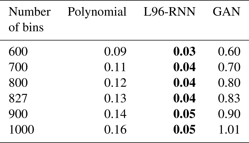
Table B2 KL divergence (goodness of fit) between (1) the truth and (2) the parameterized models, for the distributions shown in Fig. 4. The smaller the KL divergence, the better the match between the true and modelled distributions. The best model in each case is shown in bold.