Recalibration of a three-dimensional water quality model with a newly developed autocalibration toolkit (EFDC-ACT v1.0.0): how much improvement will be achieved with a wider hydrological variability?

Autocalibration techniques have the potential to enhance the efficiency and accuracy of intricate process-based hydrodynamic and water quality models. In this study, we developed a new R-based autocalibration toolkit for the Environmental Fluid Dynamics Code (EFDC) and implemented it into the recalibration of the Yuqiao Reservoir Water Quality Model (YRWQM), with long-term observations from 2006 to 2015, including dry, normal, and wet years. The autocalibration toolkit facilitated recalibration and contributed to exploring how a model recalibrated with long-term observations performs more accurately and robustly. Previously, the original YRWQM was calibrated and validated with observations of dry years in 2006 and 2007, respectively. Compared to the original YRWQM, the recalibrated YRWQM performed just as well in water surface elevation, with a Kling–Gupta efficiency (KGE) of 0.99, and water temperature, with a KGE of 0.91, while performing better in modeling total phosphorus (TP), chlorophyll a (Chl a), and dissolved oxygen (DO), with KGEs of 0.10, 0.30, and 0.74, respectively. Furthermore, the KGEs improved by 43 %–202 % in modeling the TP–Chl a–DO process when compared to the models calibrated with only dry, normal, and wet years. The model calibrated in dry years overestimated DO concentrations, probably explained by the parameter of algal growth rate that increased by 84 %. The model calibrated in wet years performed poorly for Chl a, due to a 50 % reduction in the carbon-to-chlorophyll ratio, probably triggered by changes in the composition of the algal population. Our study suggests that calibrating process-based hydrodynamic and water quality models with long-term observations may be an important measure to improve the robustness of models under severe hydrological variability. The newly developed general automatic calibration toolkit and a possible hierarchical autocalibration strategy will also be a powerful tool for future complex model calibration.

1 Introduction

Lakes and reservoirs fulfill the role of “sentinels” to climate change due to both their capacity to buffer synoptic-scale hydroclimatic extremes and their susceptibility to hydrological variability (Adrian et al., 2009; Williamson et al., 2009; Mooij et al., 2019). In recent decades, dramatic hydrological variability has been widely detected and has remarkably influenced biogeochemical processes in lakes and reservoirs (Sinha et al., 2017; Grant et al., 2021; Kong et al., 2022; Salk et al., 2022). In a bid to delve into these variations, process-based hydrodynamic and water quality models have been increasingly popular tools, since they can disentangle numerous intricate causal relations between exogenous drivers and environmental impacts within waterbodies (Arhonditsis and Brett, 2004; Mooij et al., 2010; Fu et al., 2019). However, the accuracy and robustness of these models in the face of such intense hydrological variability have become a key issue.

Driven by the purpose of better understanding physical, chemical, and biological processes, the complexity of process-based hydrodynamic and water quality models has been unabated over recent years (Robson, 2014). However, the increased complexity of the model is a mixed blessing. It indeed helps us to examine biogeochemical processes in lakes and reservoirs, but when the complexity of the model exceeds a certain level, both the accuracy and the identifiability are diminished (McDonald and Urban, 2010). Higher dimensions, more state variables, and more specific details introduce more and more parameters into models through drastic simplification of reality, which subsequently become a massive source of model uncertainty. Model calibration is one of the essential procedures in model setup to reduce the uncertainty from parameter estimations and to obtain a satisfactory parameter set to match the simulated results with observed data (Jørgensen and Fath, 2011). Although calibration has been used extensively in process-based hydrodynamic and water quality models, there are still two notable problems.

The first problem is that the manual calibration method (trial and error) commonly used in process-based hydrodynamic and water quality models is inefficient and does not guarantee optimal results. First, some steps, such as adjustment of inputs, tuning of parameters, evaluation of model performance, and visualization of outputs, subject modelers to time-consuming and tedious tasks. Second, the parameter set selected by this method may still suffer from uncertainty and interferences of subjective factors. With the development of computer technology and its subsequent application in numerical simulation methods, the automatic calibration method is burgeoning (Shimoda and Arhonditsis, 2016). Numerous modeling studies in recent decades have employed automatic calibration procedures in 2-D or lower-dimensional process-based hydrodynamic and water quality models in lakes or reservoirs (Rigosi et al., 2011; Huang, 2014; Luo et al., 2018). However, due to their high complexity and time-consuming calculation, there are few applications of automatic calibration procedures in 3-D hydrodynamic and water quality models. For example, the automated Parameter ESTimation software (PEST) was applied in the Environmental Fluid Dynamics Code (EFDC; Arifin et al., 2016), and optimization algorithms were applied in Delft3D (Xia et al., 2022; Xia and Shoemaker, 2021, 2022). The lack of automatic calibration procedures is a major hindrance to improving the efficiency of model calibration and indirectly causes the problem below. The EFDC is a general-purpose model developed for simulating three-dimensional flow, transport, and biogeochemical processes in surface water systems, including rivers, lakes, estuaries, reservoirs, wetlands, and coastal regions (Hamrick, 1992). The hydrodynamic model consists of continuity, momentum, state, and transport equations for salinity and temperature. The water quality model consists of 22 state variables and associated kinetics (Ji, 2017). More than 200 parameters which govern the above process are spread over different cards in different input files, and the model results comprise lots of output files in different formats. Despite the emergence of numerous well-established generic tools for automatic calibration, the process of linking these tools to EFDC input and output files is still cumbersome. For such a sprawling model system as the EFDC, a specific automatic calibration tool can eliminate much of the repetitive and unnecessary work. On the other hand, specific automatic calibration tools are needed to support multi-objective evaluation methods for three-dimensional model calibration, including evaluation at different locations on the horizontal plane, evaluation at different depths on the same grid, or a mixture of these objectives.

The second problem is that many models were calibrated with only short-term observations with a narrow hydrological variability and were then employed in water ecosystem management decisions or future predictions. There are hidden perils in the presumption that these calibrated models are adaptive to a wider hydrological variability. For example, in a previous study of the Spokane River and Lake Spokane model, the use of a low-flow period for calibration may result in an overestimation of in-lake total phosphorus (TP) and chlorophyll a (Chl a), and an underestimation of minimal dissolved oxygen (DO; Zhang et al., 2018a). This issue has also arisen in studies of other models (Vaze et al., 2010; Nielsen et al., 2014; Basijokaite and Kelleher, 2021). A large number of parameters is almost impossible to be constrained by a narrow hydrological variability (Janssen and Heuberger, 1995; Franks, 2009), thus triggering the equifinality problem, where several distinct parameter inputs produce the same model outputs called the “good results for the wrong reasons” (Arhonditsis et al., 2007; Paudel, 2012). Even if the final parameter set chosen by the modeler satisfies the match between model results and observations under the current hydrological variability, there is no credibility that the model will be accurate as a robust prognostic tool under a wider hydrological variability (Arhonditsis et al., 2007). Therefore, the utilization of a longer period of observations containing a wider range of hydrological years for calibration may be an important way to improve the identifiability of parameters in process-based hydrodynamic and water quality models. Benefiting from the continued accumulation of historical observations, numerous published models have been recalibrated using longer scales of data (James, 2016; Schnedler-Meyer et al., 2022). Cerco and Noel (2005) recalibrated the Chesapeake Bay model with a decade of observations, resulting in a clear improvement in modeling primary production and light attenuation. A benefit of long-term data supports is that it is possible to explore how the hydrological variability in the calibration period and its impact on the model calibration will help establish more accurate and robust models.

Long-term modeling is required to test the model's ability to reproduce ecosystems under different hydrological years. Based on the established Yuqiao Reservoir Water Quality Model (YRWQM; Zhang et al., 2013, 2015, 2019), this study aims to explore how long-term observations under a wider hydrological variability impact the model calibration with the application of automatic calibration techniques. We hypothesized that models using observations with a longer period and wider hydrological variability for calibration perform more accurately and robustly. We first developed a new R-based autocalibration toolkit for the EFDC model. Second, we recalibrated the YRWQM by the toolkit with a decadal-scale observation under three hydrological situations, namely dry, normal, and wet periods. Finally, we compared the model performance, parameters, and kinetic processes represented by parameters across the model calibration scenarios that used different split-sample approaches. These discrepancies will highlight the importance of the hydrological variability corresponding to the observed data for model calibration and deepen our understanding of biogeochemical processes in shallow lakes and reservoirs under the wide hydrological variability.

2 Materials and methods

2.1 EFDC Automatic Calibration Toolkit

The EFDC Automatic Calibration Toolkit (EFDC-ACT) was developed in this study for automating the calibration of a 3-D hydrodynamic and water quality model, EFDC, with more than 200 parameters. EFDC-ACT is a multi-parameter and multi-variable autocalibration toolkit based on R. The documentation and source code are shared and publicly available at https://doi.org/10.5281/zenodo.7438143 (Zhang and Fu, 2022). The conceptual overview of the EFDC-ACT is shown in Fig. 1. There are three main steps in EFDC-ACT, including initialization, autocalibration, and post-analysis.

Before using EFDC-ACT, the user should prepare the necessary files, including the EFDC-ACT master file, the file with comma-separated values (CSVs) that contains the parameter and variable information, the input file for the EFDC, and the CSV file containing the observations. In the initialization step, EFDC-ACT checks and loads the master file, the parameter list, and the variable list. Then EFDC-ACT generates a matrix of parameter value ranges, sets the model evaluation statistics as the objective functions, and launches the autocalibration process. More detail is in EFDC-ACT user's guide (Sect. S1 in the Supplement).

To maintain the diversity of the parameter sets while accelerating convergence, EFDC-ACT introduced the caRamel package (Monteil et al., 2020) to the autocalibration step. The caRamel package is a genetic algorithm-based multi-objective optimizer, incorporating the multi-objective evolutionary annealing simplex method (MEAS; Efstratiadis and Koutsoyiannis, 2008) and Non-dominated Sorting Genetic Algorithm II (ε-NSGA-II; Reed and Devireddy, 2004). It is suitable for highly complex, time-consuming hydrodynamic and water quality models like EFDC. EFDC-ACT controls the caRamel optimization according to the master file and feeds the parameter value range matrix into the caRamel package. The caRamel package generates the parameter set, and then EFDC-ACT passes it into EFDC and starts the calculation. At the end of the model run, EFDC-ACT calculates the statistics, based on the modeled and observed values, and passes the result back to caRamel as the objective function value. As the parameter set is adjusted, the autocalibration process is repeated until the termination criterion is reached, such as the maximum number of runs or the expected statistic results.

Automatic model evaluation is a potent tool for making models more transparent and credible (Alexandrov et al., 2011; Soares and Calijuri, 2021). To this end, EFDC-ACT provides model result extraction, statistical model evaluation, and graphical model evaluation in the post-analysis step. During the autocalibration process, the user can open the CSV files to view each iteration's parameter set and model evaluation results. After each iteration, EFDC-ACT plots the time series using modeled and observed values, thus supplying the users with a visual comparison that statistics cannot accomplish. EFDC-ACT will also output the final optimization results in a CSV file when all iterations are complete.

According to the model evaluation guidelines proposed by Moriasi et al. (2007), the statistics used to evaluate the model performance include three categories, namely standard regression (R²), dimensionless (Nash–Sutcliffe efficiency, NSE; Kling–Gupta efficiency, KGE), and error index (mean absolute error, MAE; root mean square error, RMSE; percent bias, PBIAS; ratio of root mean squared error to the standard deviation of observations, RSR). The Kling–Gupta efficiency (KGE) is included as an alternative to NSE in this study. KGE gives equal weight to bias, linear correlation, and variability, avoiding the systematic underestimating of the variability (Gupta et al., 2009).

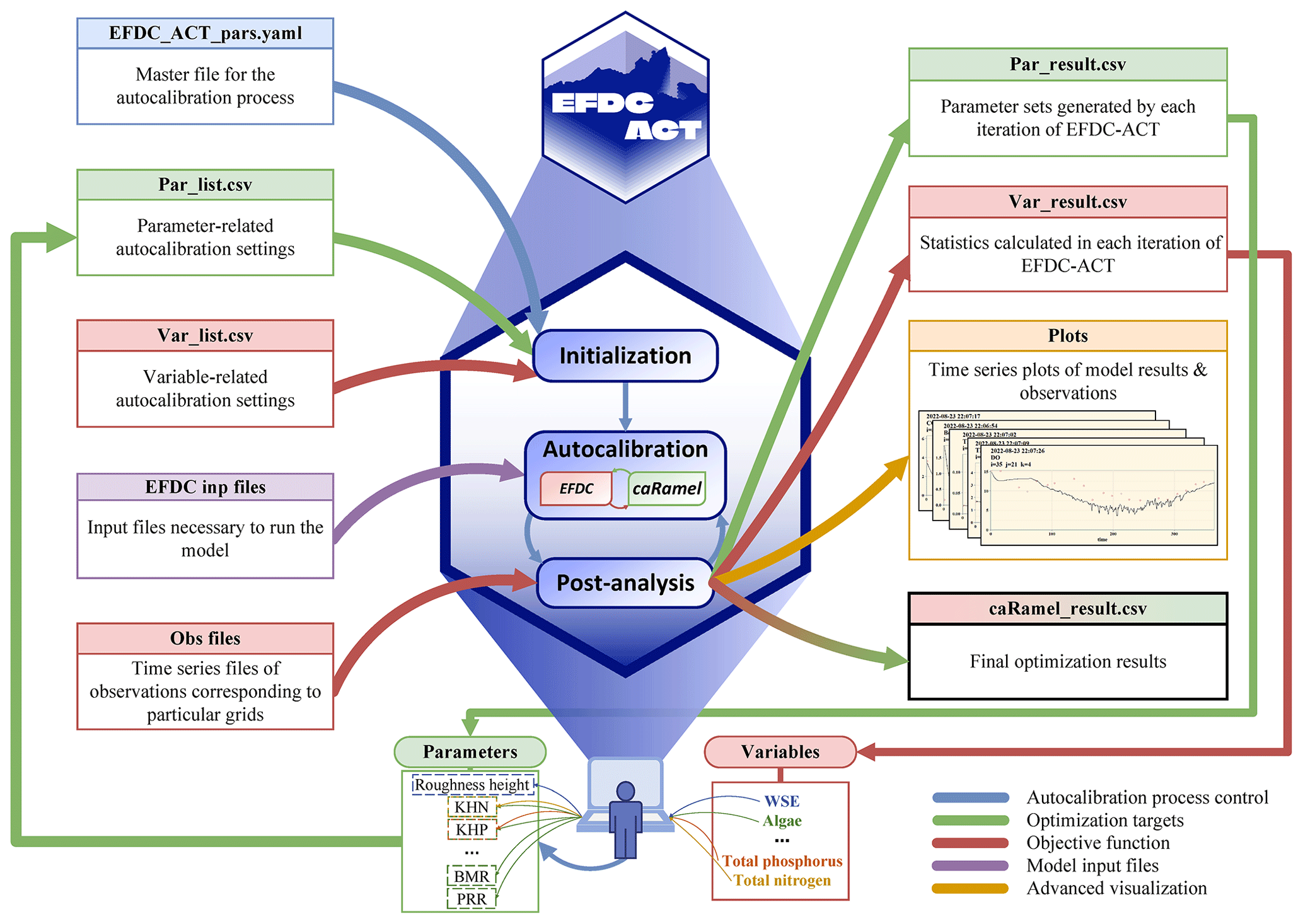
Figure 1 Conceptual overview of EFDC-ACT. The main files consist of nine categories. (a) EFDC_ACT_pars.yaml is the EFDC-ACT master file. (b) Par_list.csv indicates the parameter ranges and whether to calibrate. (c) Var_list.csv is the objective state variable, spatial location, statistics used, and accuracy expected. (d) EFDC inp files are input files for EFDC. (e) Obs files are CSV files containing observations. (f) Par_result.csv files are the autocalibration results of parameter values by each iteration. (g) Var_result.csv files are the autocalibration results of statistics for objective state variables by each iteration. (h) Plots show the time series plots for model results and observations. (i) caRamel_result.csv files are the final autocalibration results containing optimal parameter sets and model evaluations.

2.2 Chronicle of YRWQM

The Yuqiao Reservoir ($\mathrm{40}{}^{\circ }{\mathrm{00}}^{\prime }$–$\mathrm{40}{}^{\circ }{\mathrm{04}}^{\prime }$ N, $\mathrm{117}{}^{\circ }{\mathrm{26}}^{\prime }$–$\mathrm{117}{}^{\circ }{\mathrm{37}}^{\prime }$ E) is situated in Jixian county, Tianjin, China (Fig. 2). The shallow reservoir has a length of 66 km from east to west and a width of 50 km from north to south, an average water depth of 4.74 m, a maximum water depth of 12.74 m, a total surface area of 86.6 km², and a storage capacity of 1.559 × 10⁹ m³. It is situated within a basin area that covers 2060 km² (Fig. S1 in the Supplement). The Yuqiao Reservoir is the primary source of drinking, agricultural, and industrial water for approximately 129 villages in the surrounding area (Zhang et al., 2019; Yu and Zhang, 2021). Previous studies have shown that Yuqiao Reservoir is a typical mesotrophic, phosphorus-limited environment (Chen et al., 2012; Zhang et al., 2020). The YRWQM (Zhang et al., 2013) is a regional hydrodynamic and water quality model developed under the framework of EFDC (Hamrick, 1992; Ji et al., 2001) to improve the understanding and management of the Yuqiao Reservoir. Since its inception, the model has undergone five phases of development and refinement (Fig. 2).

The original YRWQM was constructed to investigate how agricultural pollution by flood flows affects the water quality in the Yuqiao Reservoir. The model was calibrated, validated, and employed to predict the variations in the water quality resulting from agricultural pollution (Zhang et al., 2013). Subsequently, the YRWQM was coupled with a modified submerged aquatic vegetation model (M-SAVM) to study the development effect of submerged macrophytes (Zhang et al., 2015, 2016) and epiphyton (Špoljar et al., 2017; Zhang et al., 2018b) on the water quality indicators of the reservoir. An integrated climate–hydrological–water quality (RCM-SWAT-YRWQM) framework was also proposed to elucidate the effects of a changing climate on the trophic state (Zhang et al., 2019).

The YRWQM has become a powerful tool for the research and management of the Yuqiao Reservoir water ecosystem through the above phases in the past decade. However, there may still be a risk of insufficient accuracy since the original YRWQM calibration does not take into account long-term hydrological variability. With the availability of the decadal-scale observations covering dry, normal, and wet periods and the design of new model calibration methods, it is time to examine whether a longer period of calibration can improve the accuracy and robustness of the model.

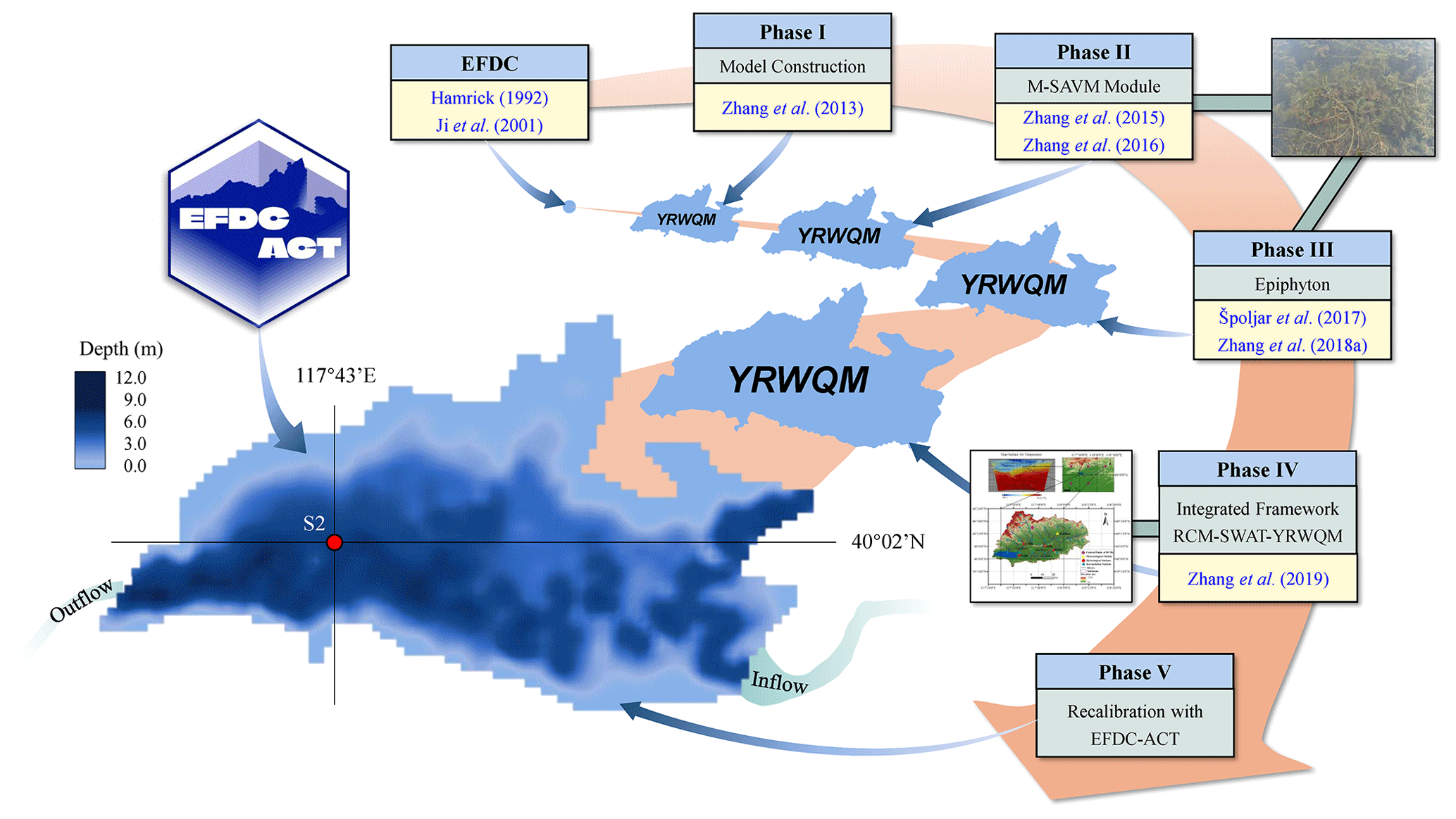
Figure 2 Bathymetric map of the Yuqiao Reservoir and the chronicle of YRWQM. The YRWQM has undergone five phases of development and refinement, including (I) model construction, (II) the M-SAVM module, (III) epiphyton, (IV) the integrated framework of RCM-SWAT-YRWQM, and (V) recalibration with EFDC-ACT.

2.3 Benchmarking point: model calibration with the strategy of the original YRWQM

As mentioned above, the original YRWQM was initially developed for the purpose of investigating the variations in the water quality arising from agricultural pollution in the Yuqiao Reservoir. Both the hydrodynamic and water quality model were calibrated and validated with the observations collected in the six monitoring stations from 2006 to 2007, and the performance was satisfactory. A more detailed description of the original YRWQM can be found in Zhang et al. (2013). It should be noted that both the calibration period (the year 2006) and validation period (6 months of the year 2007) was under dry hydrological conditions.

Consistent with the original YRWQM calibration strategy, the dry years (the years 2006, 2007, 2010, and 2015) of the decade were selected as the calibration period to establish a benchmarking point for comparison with the recalibrated YRWQM. The parameter set obtained from the calibration was implemented to simulate other years with different hydrological conditions to validate the model. The normal years (the years 2009, 2011, and 2014) and the wet years (the years 2008, 2012, and 2013) of the decade were also employed to calibrate and then validate the model with the same method. All three different models and their parameter sets were eventually compared with the recalibrated YRWQM to reveal improvements with a wider hydrological variability.

2.4 YRWQM recalibration with EFDC-ACT

The datasets required for YRWQM recalibration included meteorological data, discharge, precipitation, evaporation, water surface elevation, water temperature, and water quality data. Meteorological data are obtained from the China Meteorological Data Service Center. Discharge, precipitation, evaporation, and water surface elevation data used in the model were obtained from the Yuqiao Reservoir Administrative Bureau. The data above were collected at a frequency of once a day from 2006 to 2015, except for 2012, when water surface elevation data were collected once a month (Zhang et al., 2019). While six monitoring stations were employed by the original YRWQM for calibration and validation (Zhang et al., 2013) to balance the cost with the accuracy in calibration, water temperature and water quality data collected from monitoring station S2 were used in recalibrated model evaluation, which represented the water column at the center of the Yuqiao Reservoir. The water quality state variables included TP, Chl a, and DO concentrations (Zhang et al., 2015). All of the water quality data were sampled, preserved, and analyzed monthly or semi-monthly from 2006 to 2015, according to the Standard Methods for the Examination of Water and Wastewater editorial board.

Due to the lower stability of the hydrodynamic model compared to the water quality model, the recalibration of the YRWQM was divided into two parts, namely the hydrodynamic model recalibration and the water quality model recalibration. Both parts of the YRWQM were recalibrated with EFDC-ACT. The parameter ranges listed in Table S1 in the Supplement were referenced from the original YRWQM and other literature (Wu and Xu, 2011; Zhang et al., 2013; Yi et al., 2016; Jiang et al., 2018; Zhao et al., 2020; Kim et al., 2021). KGE and PBIAS were used to evaluate the recalibrated model. Model performance is considered satisfactory when the KGE is greater than −0.41 in this study, meaning that the model improves upon the mean value benchmark (Knoben et al., 2019). The PBIAS describes the average tendency for simulated values to be greater or less than observed values, with positive values indicating a model bias toward underestimation and negative values indicating a model bias toward overestimation (Gupta et al., 1999).

The hydrodynamic model of YRWQM was recalibrated with the field data collected between 2006 and 2015, with a time step of 10 s. The objective function of EFDC-ACT included the KGE results of water surface elevation (WSE) and surface water temperature (TEM) at station S2 from 2006 to 2015. The decade included dry years (2006, 2007, 2010, and 2015), normal years (2009, 2011, and 2014), and wet years (2008, 2012, and 2013). The parameters were automatically adjusted by EFDC-ACT until all the objective functions (KGEs) were greater than −0.41 or the number of iterations reached the maximum. In the water quality model recalibration, the objective function of EFDC-ACT included the KGE results of three water quality state variables (TP, Chl a, and DO) at station S2 from 2006 to 2015. When all the objective functions (KGEs) were greater than −0.41 or the number of iterations exceeded the maximum, the autocalibration is considered complete.

3 Results

3.1 EFDC-ACT efficiency and model recalibration

Before giving the complicated details of the analysis on model performance and parameters, we first give an overview of the implementation of the EFDC-ACT on the YRWQM recalibration. Both the manual recalibration and the automatic recalibration experiments with a modeling scale of 1 year were implemented under the same calculating workstation with an Intel^® Core™ i7-10700 CPU at 2.90 GHz. In the manual recalibration, each iteration took an average of 8.25 h, with an average of 6.41 h spent on modeling and an average of 1.84 h spent on manual pre-processing (parameter adjustment and parameter set recording) and post-processing (result extraction, statistic calculation, time series plotting, and model performance recording). The manual pre- and post-processing took 22.35 % of the total time of each iteration. In the automatic recalibration, each iteration took an average of 6.43 h, with an average of 0.02 h (77 s) spent on automatic pre- and post-processing. The automatic pre- and post-processing took 0.36 % of the total time of each iteration. In terms of time consumption, automatic recalibration with EFDC-ACT takes 21.99 % less time than the manual operation, thereby reducing the time consumed per iteration by 22.02 % (1.82 h). From the perspective of labor-saving, EFDC-ACT spared the modeler from tedious, repetitive tasks such as extraction of results, calculation of statistical values, and plotting of the time series. These savings in time and labor provided us with abundant time to analyze and improve the recalibrated YRWQM.

During the recalibration period (2006–2015), the bottom roughness height and the wind drag multiplier were automatically calibrated. The hydrodynamics of the recalibrated YRWQM demonstrated good performance for WSE and TEM at station S2 (Fig. 3). The recalibrated YRWQM remarkably reproduced the decadal variation in the WSE in Yuqiao Reservoir with a KGE of 0.99. The recalibrated YRWQM reproduced the seasonal cycle of water temperature with a KGE of 0.91. The highest and lowest water temperatures were grasped with a highest observed value of 31 ^∘C and a corresponding simulated value of 28 ^∘C and a lowest observed value of 0 ^∘C and the same corresponding simulated value. The modeled WSE and TEM both indicated that the hydrodynamic model in the recalibrated YRWQM is reliable and can be used for water quality modeling in the Yuqiao Reservoir during the recalibration period.

The water quality of the recalibrated YRWQM performed satisfactorily for the modeled TP concentration at station S2 with a KGE of 0.10. Most of the observations were evenly distributed, with little variance on either side of the modeled values (Fig. 3). The modeled TP concentration peaked at the end of 2010 and 2011 and was beyond the range of the observations. Nevertheless, the inter- and intra-annual variability in TP concentrations were still well captured, and the model showed acceptable performance overall, with a PBIAS of 40 %. The model represented the variation in the Chl a concentration over the decade, with a KGE of 0.30. The Chl a concentration showed a clear double-peaked or multi-peaked pattern in the intra-annual variation, with peaks occurring mostly in spring and autumn (Fig. 3). The modeled DO concentrations likewise showed good performance, with a KGE of 0.74. DO concentration exhibited a pronounced seasonal cycle, with lower concentrations in summer and higher concentrations in winter (Fig. 3).

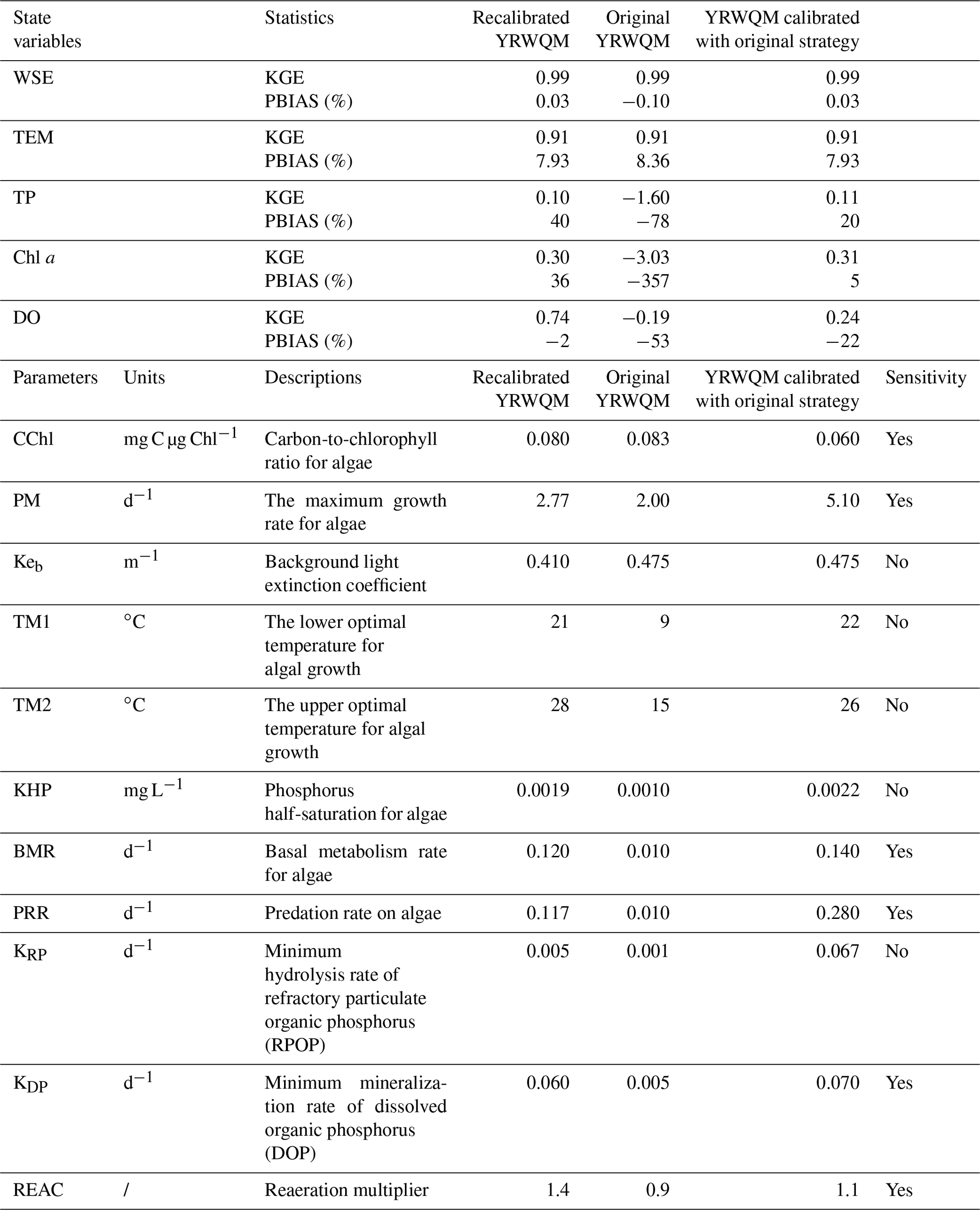
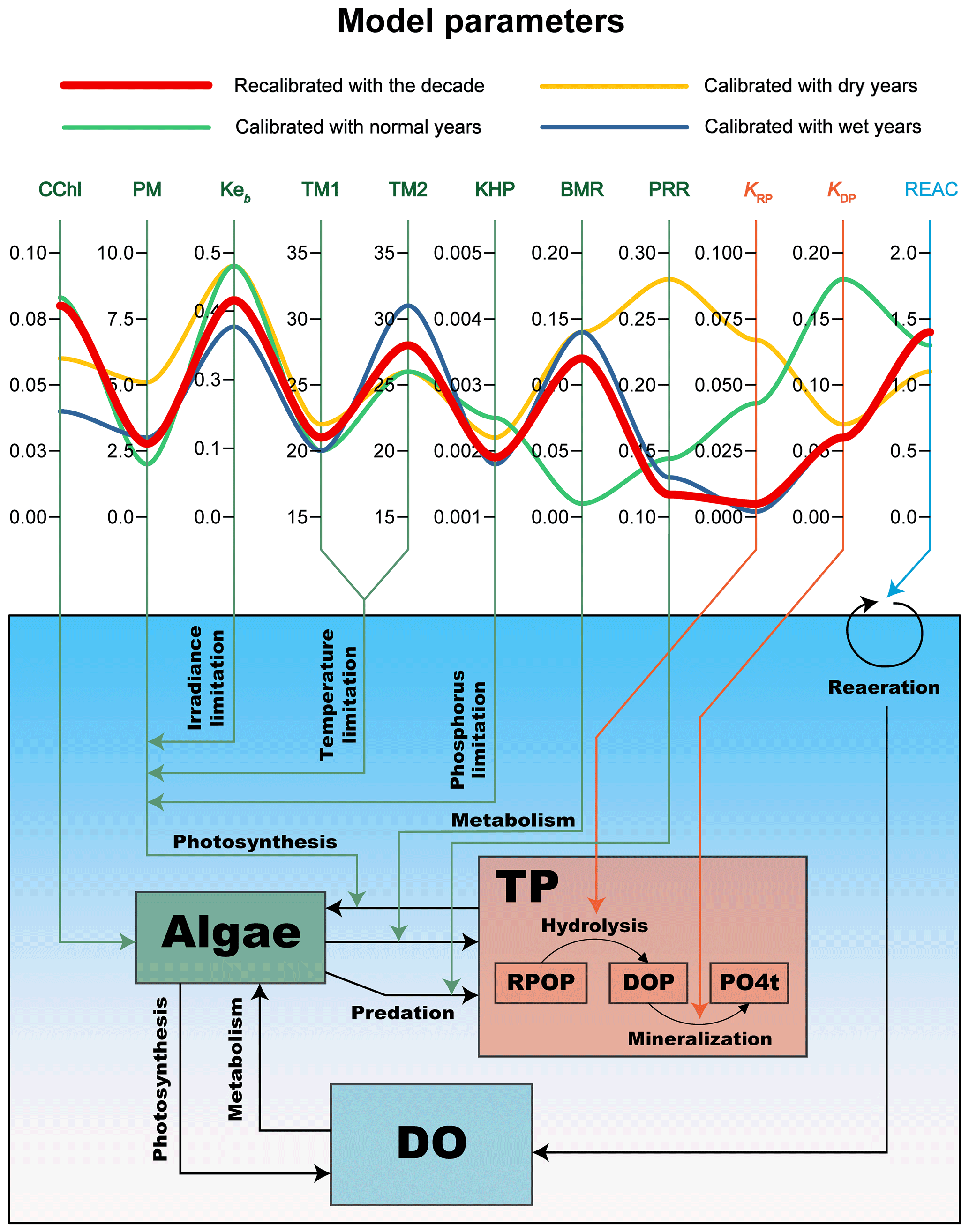
The comparisons of the recalibrated model against the original model demonstrated the better accuracy and robustness of the recalibrated YRWQM over the decade in the Yuqiao Reservoir (Table 1). The hydrodynamics of the recalibrated YRWQM performed as well as the original YRWQM, while the recalibrated YRWQM performed better than the original YRWQM in modeling the TP, Chl a, and DO concentrations. The water quality of the original YRWQM failed to reach a satisfactory result, with KGEs of −1.60, −3.03, and −0.19 for TP, Chl a, and DO, respectively, while the water quality of the recalibrated YRWQM performed well, with KGEs of 0.10, 0.30, and 0.74, respectively, as mentioned above. The 11 primary parameters in the water quality model are listed in Table 1, eight of which governed algal kinetics (CChl, PM, Ke_b, TM1, TM2, KHP, BMR, and PRR), two parameters influenced phosphorus cycling (K_RP and K_DP), and one affected reaeration (REAC). Among these parameters, we also found six of them to be sensitive (Table 1). These parameters were the carbon-to-chlorophyll ratio for algae (CChl), the maximum growth rate for algae (PM), basal metabolism rate for algae (BMR), predation rate on algae (PRR), the minimum mineralization rate of dissolved organic phosphorus (K_DP), and reaeration multiplier (REAC). These primary parameters were selected during our calibration process, based on the biogeochemical characteristics of Yuqiao Reservoir and the model performance, and they significantly influenced the model results. More detailed model equations, parameter interpretations, and calibration results are listed in Sect. S3.

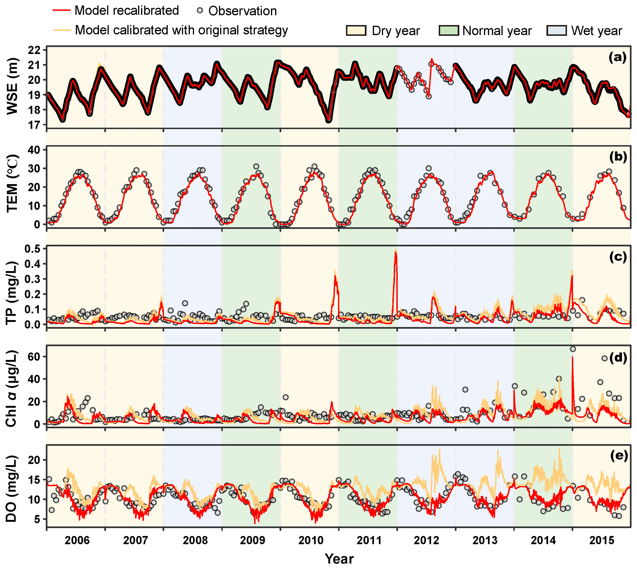
Figure 3 Performance of the model recalibrated and the model calibrated with original strategy (with dry years) at station S2 of the Yuqiao Reservoir (n=3309 for WSE and 190 for other state variables).

Table 1 Comparison of the recalibrated YRWQM, the original YRWQM (calibrated with the year 2006), and YRWQM calibrated with the original strategy (the dry years 2006, 2007, 2010, and 2015). The state variables being compared included WSE, TEM, TP, Chl a, and DO. The parameters being compared included eight governing algal kinetics (CChl, PM, Ke_b, TM1, TM2, KHP, BMR, PRR), two influencing phosphorus cycling (K_RP and K_DP), and one affecting the reaeration of DO (REAC). A more detailed explanation of the model equations and parameters is listed in Sect. S3.

3.2 Performance comparison between YRWQM recalibrated by decade and models calibrated with different hydrological years

There were obvious discrepancies in the performance of the recalibrated YRWQM in different hydrological years (Fig. 4). The ability of the recalibrated YRWQM to reproduce TP concentrations for the decade was the best, with the highest KGE values. The recalibrated model evaluation for TP concentrations reflected a satisfactory performance in dry and wet years, with KGEs of −0.22 and 0.004, respectively, while in normal years the KGE value was less than −0.41. The recalibrated model showed reasonable performance for Chl a concentration and performed best in normal years, with a KGE of 0.36. The recalibrated model succeeded in reproducing DO concentrations in different hydrological years, with all KGE values greater than 0.6 and the maximum KGE of 0.76 occurring in wet years.

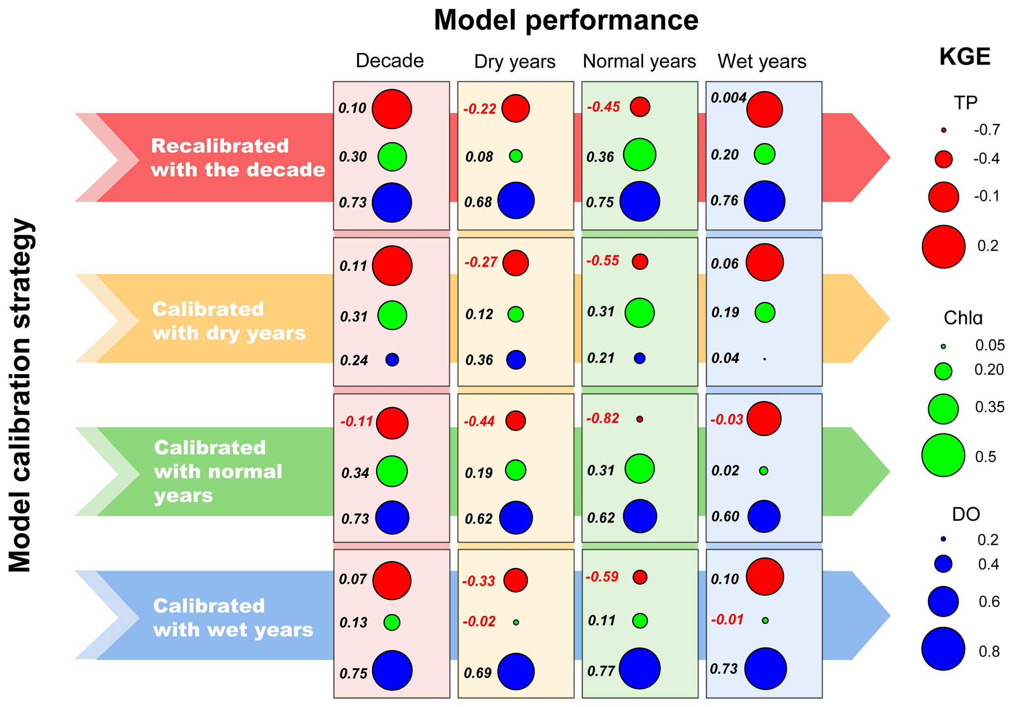
Figure 4 Performance of the models calibrated with different strategies. The YRWQM was recalibrated with the decade and calibrated with dry, normal, and wet years, respectively. The parameter sets derived from four model calibration strategies were applied to the other hydrological years or the decade to validate the model under the different hydrological conditions.

In comparison to the YRWQM recalibrated with the decade, the other three models calibrated in different hydrological years showed distinct inferiority (Fig. 4). The model calibrated in dry years had a relatively poor performance when modeling DO, with a KGE of 0.24 for the decade and a maximum KGE of 0.36 in dry years. The model calibrated in normal years failed to obtain good evaluations in modeling TP, with the lowest KGE values for the decade and in all three different hydrological situations. The model calibrated in wet years showed relatively worse results when modeling Chl a, with all KGE values being less than 0.2 and the lowest KGE of −0.02 occurring in dry years. The results indicated that the YRWQM recalibrated with the decadal information outperformed the other three models calibrated with a single hydrological year, with the best robustness in modeling TP, Chl a, and DO concentrations for a wide hydrological variability during the decade.

3.3 Parameters and kinetic processes comparison between recalibrated YRWQM and models calibrated within different hydrological years

Similar to the model performances, models employing different calibration strategies also had different parameter results (Fig. 5). Most parameter values of the recalibrated YRWQM were within the parameter ranges of the other three calibrated models, except for PRR, which had the lowest value of 0.12 among the four models. PRR represents the rate of predation on algae by zooplankton or other aquatic organisms, and algal predation is one of the main causes of algal reduction.

Compared to models using other calibration strategies, the model calibrated in dry years had the highest PM of 5.1, the highest PRR of 0.28, and the lowest REAC of 1.1. PM and PRR govern the growth and predation of algae, respectively. REAC represents the reaeration multiplier for the turbulence-induced and wind-induced surface reaeration coefficient, and a lower REAC value means less reaeration at the air–water interface. There were significantly lower BMR and higher K_DP in the model calibrated in normal years, and these are the two parameters that represent the algal basal metabolism and the mineralization of dissolved organic phosphorus into inorganic phosphorus, respectively. Most parameters of the model calibrated in wet years were similar to the model recalibrated in the decade, except for one significantly lower value of CChl, which governs the conversion between the modeled and measured algal biomass.

Figure 5 Parameters of the models calibrated with different hydrological years.

4 Discussion

4.1 Recalibrated YRWQM vs. original YRWQM

Before embarking on the discussion of the discrepancies between the recalibrated YRWQM and original YRWQM, it is important to note that the model evaluations chose a single station (station S2 at the center of the Yuqiao Reservoir) and three state variables (TP, Chl a, and DO), which are constrained by the complexity and computational cost of decadal-scale modeling. Nevertheless, the above indicators were considered to be capable of representing the main biogeochemical processes in Yuqiao Reservoir, as previous statistical analyses and numerical models have indicated that Yuqiao Reservoir is a phosphorus-limited mesotrophic reservoir (Chen et al., 2012; Zhang et al., 2013; Xu et al., 2015). The model evaluations demonstrated that the recalibrated YRWQM performed equally well when compared to the original YRWQM in terms of hydrodynamics, while the recalibrated YRWQM outperformed the original when it came to water quality. We supposed that the better performance probably stemmed from the recalibrated parameter values, especially for sensitive parameters (Table 1). As described by Cerco and Cole (1994) in the three-dimensional eutrophication model of Chesapeake Bay, the growth rate of algae was expressed as a multiplication of the maximum growth rate (PM), with a series of limiting factors in YRWQM, while the algal reduction was caused mainly by basal metabolism (BMR) and predation (PRR). These parameter values in the original YRWQM gave the algae growth conditions that were too lenient and motivated inaccurate algal outbreaks during the decade, with a PBIAS of −357 % (Table 1). These algal outbreaks may also be a potential reason for the overestimations of TP and DO concentrations with PBIAS values of −78 % and −53 %, respectively (Table 1). With the excessive algal outbreaks in the original YRWQM, the continuous enrichment of phosphorus in algae and the oxygen production process of excessive net photosynthesis prompted the final overestimations (Ji, 2017). As algal kinetics were accurately parameterized during the decade, with a PBIAS of 36 % in the recalibrated YRWQM, satisfactory results were also obtained for TP and DO concentrations, with PBIAS values of 36 % and −2 %, respectively (Table 1).

It should be noted that the modeled TP concentration peaks were not recorded in the observations in late 2010 and 2011 (Fig. 3). This may have been caused by the year-end water transfer, with inflow TP concentrations reaching 460 and 960 µg L⁻¹ in December 2010 and 2011, respectively. It may also demonstrate that the recalibrated YRWQM can provide a higher temporal resolution than observations and has potential as a hindcast model for reservoir management. Overall, the accuracy and robustness of the YRWQM have taken a solid step forward over a meticulous, long-term recalibration process with EFDC-ACT.

4.2 Why does the recalibrated YRWQM have better-performing parameters? Impact of the hydrological variability on calibration results

Although it has been discussed above how updating parameter values improved the model accuracy and robustness of YRWQM, it is now more intriguing to see how this parameter update was achieved by recalibration. We suppose that the observations with a wide hydrological variability may have contributed to the better-performing parameters, as the original YRWQM was calibrated and validated in the only dry situation, while the recalibrated YRWQM used decadal observations with a wide range of hydrological variability. Hydrological variability is one of the main causes of varying biogeochemical processes (Delpla et al., 2009; Li et al., 2020), and the changes in parameter values reflect the variability in these processes (Robson et al., 2018). James (2016) recalibrated the Lake Okeechobee Water Quality Model, using 30 years of observations, including a series of extreme hydrometeorological events, thereby improving the quality of the parameters and the ability to model nitrogen and phytoplankton. Many studies have also shown that the improvement in the model parameters may be triggered by the calibration using long-term observations with greater hydrological variability (Cerco et al., 2004; Lung and Nice, 2007).

Among the four models, the parameters of the recalibrated YRWQM showed a proper trade-off, with values almost falling within the range determined by the other models calibrated in specific hydrological years (Fig. 5). The model calibrated in dry years performed as well as the recalibrated YRWQM for Chl a but failed to reproduce DO, with a PBIAS of −21 % (Fig. 4). This may be due to the highest algal growth rate (PM) causing excessive net photosynthesis (Fig. 5). The drastic water level fluctuations in the Yuqiao Reservoir in dry years (Fig. 3) probably caused the decline of the submerged macrophytes and the increase in the phytoplankton, like for other shallow waterbodies (Furey et al., 2004; Krolová et al., 2013; Lu et al., 2018). However, it is necessary to analyze more observations of submerged macrophytes and couple the recalibrated YRWQM with M-SAVM to gain a definite conclusion (Zhang et al., 2015). In the case of the model calibrated in wet years, the model performed poorly in modeling Chl a (Fig. 4), and the carbon-to-chlorophyll ratio (CChl) was the lowest (Fig. 5). Unlike a fixed value in the model, the value of CChl is more variable and depends on the makeup of the algae population, typically ranging from 0.015 to 0.1 (Bowie et al., 1985). Ren et al. (2019) also noted the differences in microbial composition between the dry and wet periods in Poyang Lake. A multi-species phytoplankton module that enables variable CChl may contribute to more robust algal modeling. The above discussion pointed out the risks inherent in employing a model calibrated with a single hydrological year for climate change studies or management decisions. Regarding the point of model accuracy and robustness, the use of long-term observations with sufficient hydrological variability to calibrate hydrodynamic and water quality models is probably the best option.

4.3 Highly efficient calibration with EFDC-ACT

The newly developed autocalibration toolkit, EFDC-ACT, eliminated a lot of hindrances in the recalibration of YRWQM. Compared to the conventional manual calibration method, it not only reduces a great deal of uncertainty from the subjective choice of parameters but also accelerates the convergence of the optimization process. As a generic autocalibration toolkit developed for models based on the EFDC framework, the EFDC-ACT supports the autocalibration of any combination of more than 200 parameters in the EFDC model. Meanwhile, the EFDC-ACT also incorporates automatic model evaluation and advanced visualization of simulations and observations. Some process patterns can only be seen by time series plots and 2-D plots. Statistics alone cannot reveal this kind of pattern (Bennett et al., 2013; Hipsey et al., 2020). The automated time series plots make the model results more visual and transparent at this point. The generated output files after each optimization iteration are overwritten, and only the model parameters and evaluation results of each iteration are retained. This design ensures reproducibility, while avoiding the need for a large volume of hard disk space (Luo et al., 2018). The entire automatic calibration framework proposed with EFDC-ACT can also be a reference to develop other automatic calibration tools for hydrodynamic and water quality models.

The caRamel algorithm adopted in EFDC-ACT has been demonstrated through case studies to obtain similar optimization results, while speeding up convergence (Monteil et al., 2020). However, hundreds of parameters and the high spatial and temporal complexity of EFDC bring about a time-consuming computation, making it difficult to reach the recommended number of iterations for the caRamel algorithm. Furthermore, even with the support of optimization algorithms, how to obtain better calibration results faster is still a critical issue for the autocalibration of high-complexity models like EFDC. However, with the aid of autocalibration, modelers should spend time learning and understanding the model system and the parameter implications to avoid getting good model error statistics values with the wrong parameters. The autocalibration should be viewed as an efficient way to refine the calibration after learning the model system with the manual calibration.

4.4 Challenging high-complexity model autocalibration problems: a possible hierarchical autocalibration strategy introducing expert knowledge

To enable faster convergence of the model parameter optimization process, we propose a hierarchical autocalibration strategy based on EFDC-ACT. This strategy requires the modelers to calibrate the model three times, for different purposes, in an orderly and automatic manner. First, modelers formulate a large range of parameters based on the literature or parameter implications and then run EFDC-ACT and perform a sensitivity analysis to find both the sensitive parameters and state variables. Although EFDC-ACT does not provide the functions for sensitivity analysis, there are a few R packages for sensitivity analysis, such as the sensitivity package. A Bayesian framework integrating sensitivity, uncertainty, and identifiability analysis was also proposed for EFDC (Jia et al., 2018). The modelers will analyze the interactions between these sensitive variables according to expert knowledge, and variables with controlling effects will be the primary target for the second level of autocalibration. Next, the modelers target the sensitive variables and parameters identified in the first round and perform the autocalibration again until the model performs satisfactorily. Finally, the modelers hold the identified variables and parameters constant and then autocalibrate the model a third time to determine the other insensitive state variables and parameters. With this hierarchical autocalibration strategy, EFDC-ACT can handle the parameter estimation of EFDC more competently. This strategy is a possible framework in the future, which is suitable not only for EFDC-ACT but also for other automatic calibration tools that do not produce sufficient iterations.

Even in the context of rapid advances in computer technology, expert knowledge is still indispensable for the calibration of highly complex models (Wood et al., 1990; Ostfeld and Salomons, 2005). With the emergence of automatic calibration tools, how to combine expert knowledge with them has become a new issue (Krueger et al., 2012; Xia and Shoemaker, 2022). The selection of key state variables in the hierarchical autocalibration strategy above is an example of the application of expert knowledge in an autocalibration tool. With the evolution of computer technology, the development of autocalibration tools, and the accumulation of observations, the hierarchical autocalibration strategy proposed above offers a possible workaround to deal with enormous autocalibration problems in high-complexity models.

5 Conclusions

We developed a new automatic calibration toolkit, EFDC-ACT, and implemented it into the recalibration of the YRWQM with 10 years (2006–2015) of observations in a wide range of hydrological variability. In comparison with the original YRWQM, the hydrodynamics of the recalibrated YRWQM performed just as well for the decade, while the recalibrated model performed significantly better in modeling TP, Chl a, and DO concentrations. When compared to the models calibrated with only dry, normal, and wet years, the KGEs improved by a maximum of 196 %, 134 %, and 202 % in modeling TP, Chl a, and DO, respectively. Our analysis indicates that the recalibrated YRWQM accuracy and robustness improvement is derived from the constraining effect of observations with a wider hydrological variability. Such information will help to unravel how hydrological variability in the calibration periods affects the process-based hydrodynamic and water quality models, including their parameters, kinetic processes, performance, and long-term robustness. Moreover, a general autocalibration toolkit developed in this study, EFDC-ACT, is substantially less time-consuming and more efficient for modelers than the conventional manual calibration method. The framework of EFDC-ACT and a possible hierarchical autocalibration strategy can also be a reference for future complex hydrodynamic and water quality model calibration. Finally, with our convenient autocalibration toolkit, it will be possible to explore the impact of the hydrological variability on more complex process-based hydrodynamic and water quality models.