the Creative Commons Attribution 4.0 License.
the Creative Commons Attribution 4.0 License.
 | 11 Jul 2023
Developing spring wheat in the Noah-MP land surface model (v4.4) for growing season dynamics and responses to temperature stress
Zhe Zhang
Fei Chen
Phillip Harder
Warren Helgason
James Famiglietti
Prasanth Valayamkunnath
Cenlin He
Zhenhua Li
The US Northern Great Plains and the Canadian Prairies are known as the world's breadbaskets for their large spring wheat production and exports to the world. It is essential to accurately represent spring wheat growing dynamics and final yield and improve our ability to predict food production under climate change. This study attempts to incorporate spring wheat growth dynamics into the Noah-MP crop model for a long time period (13 years) and fine spatial scale (4 km). The study focuses on three aspects: (1) developing and calibrating the spring wheat model at a point scale, (2) applying a dynamic planting and harvest date to facilitate large-scale simulations, and (3) applying a temperature stress function to assess crop responses to heat stress amid extreme heat. Model results are evaluated using field observations, satellite leaf area index (LAI), and census data from Statistics Canada and the United States Department of Agriculture (USDA). Results suggest that incorporating a dynamic planting and harvest threshold can better constrain the growing season, especially the peak timing and magnitude of wheat LAI, as well as obtain realistic yield compared to prescribing a static province/state-level map. Results also demonstrate an evident control of heat stress upon wheat yield in three Canadian Prairies Provinces, which are reasonably captured in the new temperature stress function. This study has important implications in terms of estimating crop yields, modeling the land–atmosphere interactions in agricultural areas, and predicting crop growth responses to increasing temperatures amidst climate change.
- Article
(11940 KB) - Full-text XML
-
Supplement
(405 KB) - BibTeX
- EndNote


Wheat is a widely grown temperate cereal and a major staple crop for global food security, ranked fourth among commodity crops, with a global production of 711×106 t. The Prairie Provinces in Canada (Alberta, Saskatchewan, Manitoba) and the US Northern Great Plains are known as the breadbasket of North America, producing spring wheat, which is the first and third largest commodity crop in Canada and the US, respectively. At the same time, Canada and the US account for approximately 20 % of the global wheat export market, according to the Economic Research Service (ERS) of the US Department of Agriculture and Agriculture and Agri-Food Canada (AAFC) (ERS USDA report, 2022; Statistics Canada; and AAFC).
Spring wheat is planted in late spring after snowmelt and soils have drained sufficiently to allow fieldwork and is harvested in late summer to avoid early fall frost. The spatial and temporal variability of climate across the entirety of the spring wheat production area of the Northern Great Plains means planting typically starts in early April in the southern portions and concludes by late May in the northern portions. Within the growing season, four major growing stages are identified for spring wheat, including seedling, emergence, anthesis, and grain filling, largely aligned with the spring and summer weather. Thus, weather variations, especially temperature, play an important role in the environmental control at each growing stage. Accumulated heat, calculated though growing degree day (GDD) accumulation, is an effective proxy to quantify crop stage.
Wheat is sensitive to high-temperature stress, whose negative impacts have been reported, particularly under the higher-end emission scenario (Lobell et al., 2011a; IPCC, 2014; Qian et al., 2019; Agyeman et al., 2021). When the temperature exceeds the optimal range, it can have three main effects: (1) the high temperature can lead to the closure of leaf stomata, reducing CO2 absorption and transpiration and increasing photorespiration competition, which lowers photosynthetic efficiency; (2) the high temperature can impair the activity of enzymes in leaf chloroplasts; (3) and the high temperature can shorten phenological developments, particularly during the grain-filling stage, affecting biomass accumulation. These processes will reduce crop photosynthesis at the physiological level and affect crop phenological development.
As such, it is important to understand and accurately represent growing dynamics and responses to heat stress for spring wheat, from plant physiology to its parameterization in Earth system model applications. Previous studies have utilized statistical regression models to connect agricultural production with weather inputs. Usually, the spatial region for each regression model is large and there is a lack of detailed process understanding in these statistical studies (Qian et al., 2009; Carew et al., 2017). Ensemble process-based crop model studies (e.g., AgMIP study, Rosenzweig et al., 2013; Jägermeyr et al., 2021) have applied statistical downscaled forcing from ensemble general circulation models (GCMs) to demonstrate the impacts of climate change on crop production (Semenov and Shewry, 2011). Although studies provided important quantification of the uncertainty range originating from GCM forcing, RCP scenarios, and crop model parameterizations, this approach has simplified processes for complex energy, water, and carbon interactions occurring on the surface during crop growing seasons, including their potential feedback to the atmosphere.
There is an emerging trend for physical process-based crop models integrated within Earth system models (ESMs) to specifically investigate dynamic crop growth and heat response under climate change (Levis, 2014; McDermid et al., 2017). In particular, the Noah-MP crop model (Liu et al., 2016) integrates dynamic crop growth processes of two major crops, corn and soybean, into simulation of surface energy, water, and carbon fluxes (Niu et al., 2011; Yang et al., 2011) and can be further coupled with the Weather Research and Forecasting model (WRF, Skamarock et al., 2008) for regional climate simulations. In addition, Xu et al. (2019) incorporated an irrigation scheme based on soil moisture deficit, and these two schemes were jointly tested in Zhang et al. (2020b) for the US Midwest Corn Belt and Mississippi River valley with reasonable performance. As the third largest crop planted in the US and Canada, the dynamic growing process of wheat is not yet developed in the Noah-MP land surface model (LSM), calling for better representation of wheat growing processes.
This study has three goals: (1) develop a dynamic wheat growth model in the Noah-MP crop from the Kenaston site in Saskatchewan, (2) conduct large regional wheat simulations for the Northern Great Plains and Canadian Prairies, and (3) address the temperature response function and investigate the impact of heat stress on crop yield in this region. The structure of this paper is as follows: Sect. 2, “Model and data”, will introduce the Noah-MP crop model and the necessary data used in this study. Section 3, “Results”, will present the results from three designed simulations – a single-point model, large regional simulations, and accounting for heat stress function. Section 4 provides a broad discussion of discrepancies between model results and evaluation datasets, planting/harvest practice in real agricultural management, and the temperature stress function. The final conclusions are discussed in Sect. 5.
2.1 Noah-MP crop model
In this study, we mainly used the inherent model structure in the Noah-MP crop model; added a new crop species, spring wheat; and developed new features, such as a dynamic planting/harvest date for regional application, as well as investigating the crop responses to high temperature. The Noah-MP LSM is widely used for modeling land surface processes, energy and water balance, and the land surface component coupled with regional weather and climate model (WRF). The crop model in Noah-MP was initially developed in Liu et al. (2016) to accommodate corn and soybean, two major crops grown in the US. Zhang et al. (2020b) performed a joint crop and irrigation simulation for these two crop species in the US for large regional-scale application.
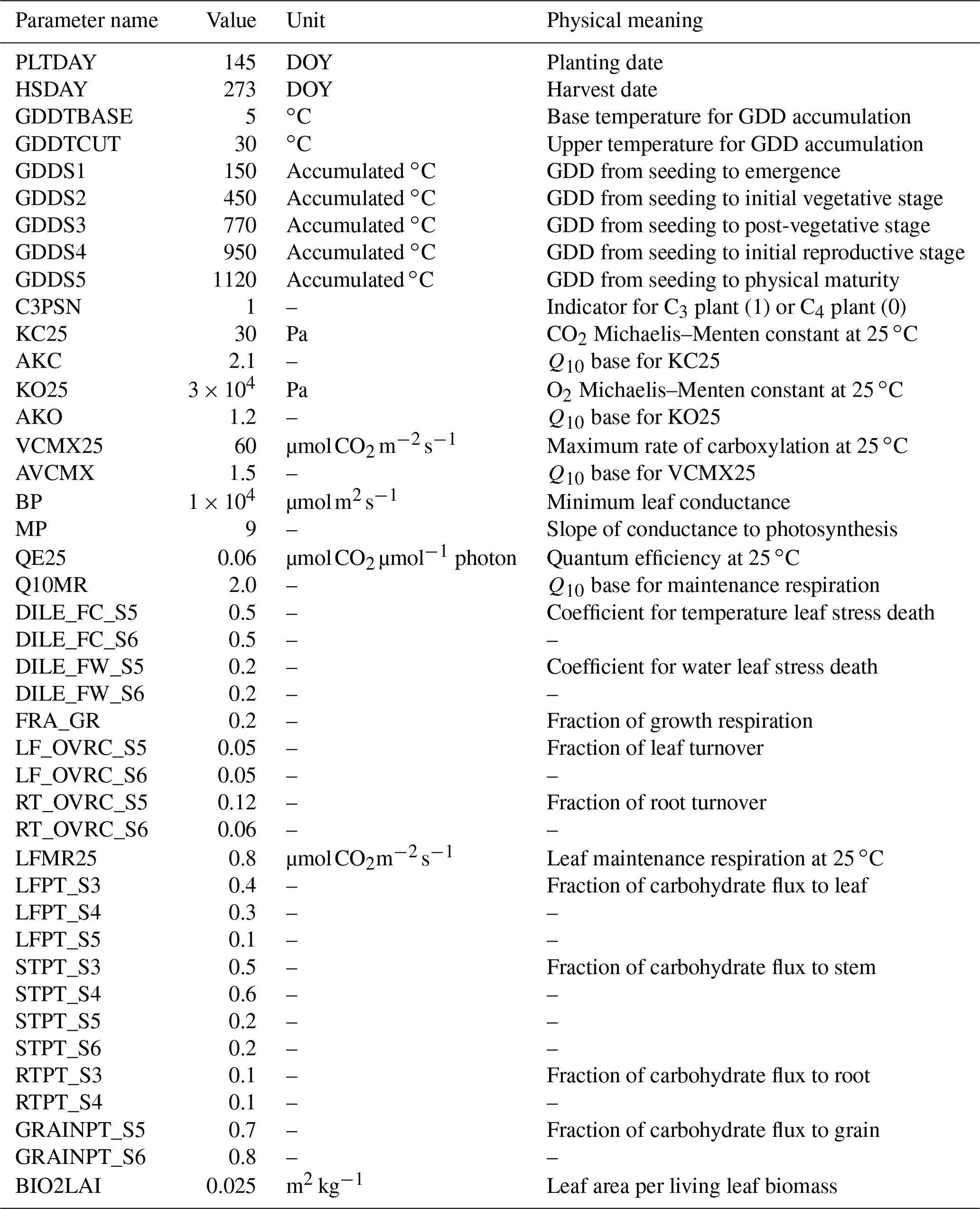
The Noah-MP crop model has three main components, the photosynthesis–stomata component, the growing degree day (GDD) component, and the carbohydrate allocation component. The photosynthesis (PSN)–stomata component calculates the CO2 assimilation and stomatal conductance, given environmental conditions, such as radiation, CO2 level, temperature, moisture stress, and plant leaf area index (LAI). This photosynthesis–stomata component contains the key processes in which the crops are actively impacted by and respond to environmental conditions. The GDD component accumulates the daily GDD (Eq. 1) and determines the crop growing stages, according to temperature and GDD thresholds for each stage set in the parameter table. The carbohydrate allocation component partitions assimilated carbohydrates (converted from assimilated CO2 from photosynthesis) to different parts (leaf, stem, root, and grain) of the plant structure, depending on the growing-stage function, with feedback between LAI and photosynthesis. These three components together constitute complete plant growing processes in phenology, physiology, biogeophysics, and biogeochemistry. Please see Appendix A for the full parameter table adjusted for spring wheat growth.
GDDTBASE (5 ∘C) and GDDTCUT (30 ∘C) are the commonly used base and cutoff temperature parameters for wheat GDD accumulation (Saiyed et al., 2009).
ACGDD is the accumulated daily GDD within the growing season. When ACGDD passes through growing-stage thresholds, the crop enters different stages, including emergence, the initial vegetative stage, the reproductive stage, maturation, and harvest. The threshold parameters determining these stages are presented in Appendix A.
2.2 Dynamic planting and harvest dates
The model spring wheat growing season is determined by the planting and harvest dates. For a starting point, they can be prescribed from field records in single-point simulations. For large-scale simulations, two approaches are adopted in this study. The first approach is to use the spatially varying values from the most common planting/harvest date for each state and province in US and Canada, respectively (USDA National Agricultural Statistics Service (NASS), 2010, province/state-level static map). This static map is shown in Fig. 1.
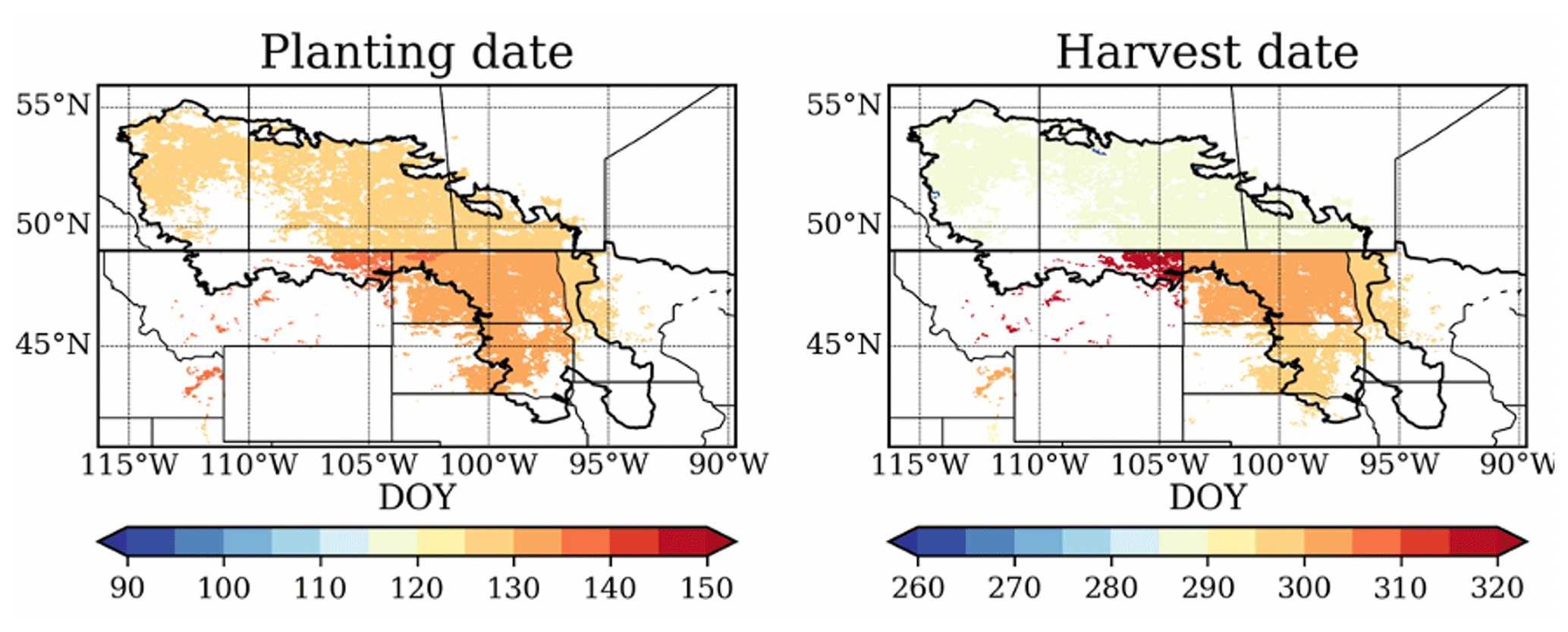
Figure 1Province/state-level planting and harvest map for DOY (day of year) in the Canadian Prairies and Northern Great Plains region.
The second approach is introducing dynamic planting and harvest, based on meteorological input, most importantly temperature. Sacks et al. (2010) provided a global synthesis of planting and harvest dates across the globe and indicated that the mostly likely planting temperature in the Canadian Prairies is around 10 ∘C and the accumulated GDD for harvest is about 1500. Sensitivity tests on these two parameters are conducted for the year 2007 and compared with the USDA weekly crop progress report; please see the Supplement for details. Iizumi et al. (2018) attempted to model the planting and harvest window for major global crops and demonstrated that environmental factors controlled by temperature and precipitation, as well as by soil moisture and snowpack, play important roles in determining the planting and harvest timing.
Similar environmental thresholds are applied in this study for both planting and harvest.
Planting is triggered by 5 d running average temperature (TAVE(5)) greater than 10 ∘C.
Harvest is triggered when accumulated GDD (ACGDD) passes 1500.
2.3 Temperature stress function
Regarding the plant physiological response to temperature, a stress function has been applied in the photosynthesis–stomata subroutine in the Noah-MP crop, originally from Collatz et al. (1991):
Equation (5) represents the temperature stress function itself; vegetation canopy temperature (TV) is used in this equation, plotted as the black dotted line in Fig. 2a. Equation (6) shows the combined temperature stress function with the temperature increase for the Vcmax25, a parameter describing the rubisco capacity enzyme at a temperature of 25 ∘C, which increases exponentially (base at 2.4) with every 10 ∘C temperature increase. This exponential increase function is also known as the Q10 function (). The combined effect of the Q10 exponential increase and temperature stress f(TV) is plotted in Fig. 2b. This combined effect of temperature on rubisco capacity shows a one-peak function which is optimal at about 33 ∘C.
However, this temperature is much higher than the actual optimal temperature for wheat growth (25–30 ∘C), due to the exponential increase from the Q10 function in Eq. (6). It is suggested that the rubisco parameter Vcmax25 displays a decrease at higher temperatures (Harley and Tenhunen, 1991; Bernacchi et al., 2013) and that Eqs. (5) and (6) can be integrated together, therefore omitting the Q10 function from Eq. (6). Wang and Engel proposed an alternative temperature stress function from a synthesis of 29 widely used wheat models, also known as the Wang–Engel temperature function (Wang et al., 2017) (Eq. 7). This new equation is visualized as the blue line in Fig. 2a and b and has a peak near 27 ∘C, a more reasonable range compared to Eq. (6) (Collatz et al., 1991). This heat stress function is adopted in the third experiment in this study (Sect. 2.6).
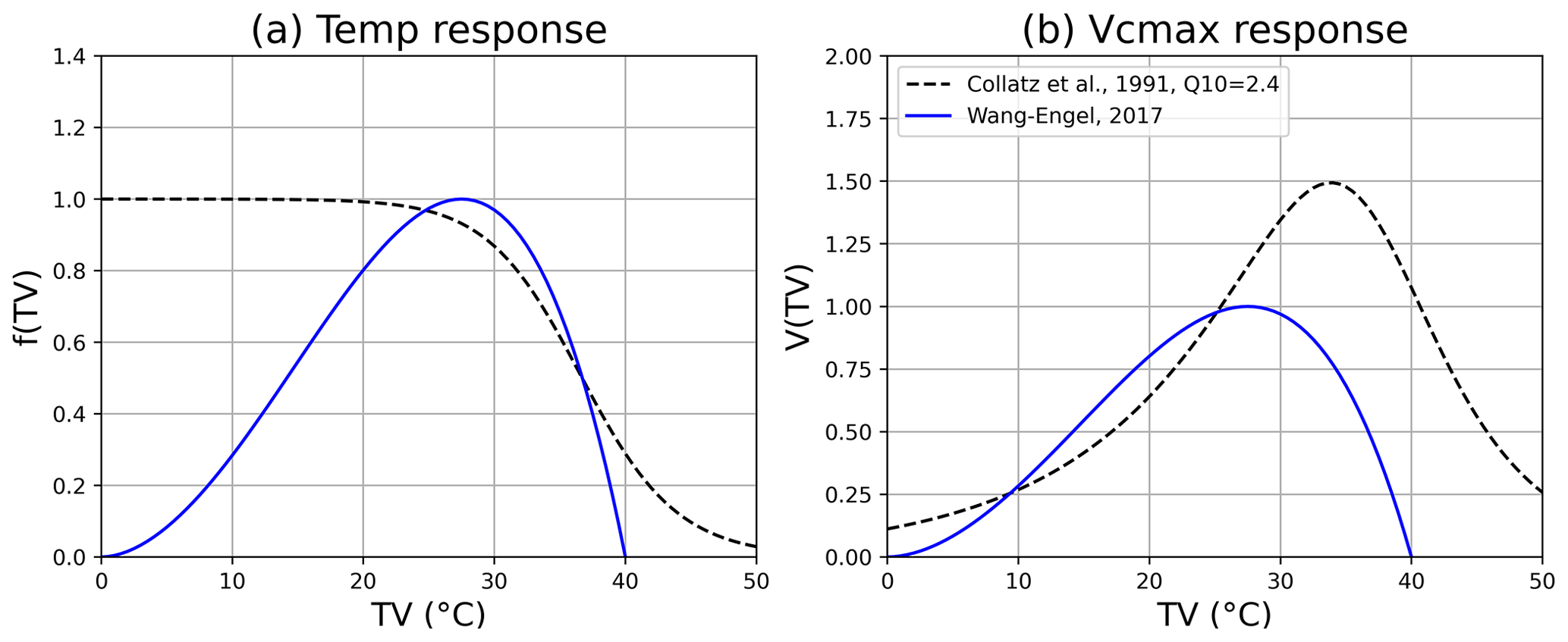
Figure 2(a) Temperature response of the default Noah-MP PSN–stomata scheme (Collatz et al., 1991) and a new temperature response function (Wang et al., 2017) revised equation; (b) rubisco capacity (Vcmax25) parameter responses to vegetation canopy temperature (TV).
2.4 Kenaston site
Observational data come from sites in the Brightwater Creek watershed located 80 km south of Saskatoon, Saskatchewan, Canada. The Agricultural Water Futures project of the Global Water Futures program (https://gwf.usask.ca/projects-facilities/all-projects/p3-ag-water-futures.php, last access: October 2022) since 2016 has collected agricultural water use and energy fluxes data for several crop species, including wheat, barley, canola, lentils, peas, and forages. These sites exhibit characteristics consistent with dryland agricultural production in the Canadian Prairies. Three site years of data for wheat specifically were collected in 2016 and 2019 at the SE13 site (51.389∘, −106.437∘) and in 2019 at the SW30 site (51.420∘, −106.422∘). Soils range between silt loam at SE13 and clay loam at SW30, and limited topography and runoff tends to restrict surface water redistribution to local depressions. Observations are focused on quantifying land–atmosphere water and energy exchange, soil moisture dynamics, and crop growth metrics.
Data included in this study include turbulent fluxes, sensible heat (SH), and latent heat (LH), as observed with eddy covariance. Campbell Scientific CSAT3 sonic anemometers and EC150 gas analyzers or Irgason (an integrated CSAT and EC150) systems collected high-frequency observations with data processing and QA QC completed with default settings in Li-Cor EddyPro software. Gap filling and energy balance closure were completed with the REddyProc packages (Wutzler et al., 2018) in R to generate a continuous 30 min time series of SH and LH observations. Soil moisture observations at two depths (5 and 20 cm) were collected with Stevens HydraProbe instruments. Due to salinity interactions, especially at the SE13 site, absolute values need to be treated with caution, while relative dynamics are more meaningful to validate model dynamics. Crop growth metrics, aboveground biomass and LAI, were collected during site visits every 2 weeks. The biomass sampling protocol provides an average value for each date from the removal of all aboveground biomass, subsequent oven drying, and weighing of between 6 and 12 samples with each sample having a 0.25 m2 ground surface extent. LAI was sampled with a Decagon AccuPAR LP-80 ceptometer. The reported value comes from the average of 20 samples taken perpendicular and parallel to crop rows every 3 m over a 30 m transect adjacent to the eddy covariance station. Care was taken to ensure stable sky conditions over the course of observations within 2 h of solar noon.
2.5 Regional data for agricultural management and model evaluation
We further expanded the single-point model to cover a large wheat-planting region across the US and Canada, according to the latest planting area data acquired from crop inventory data. The George Mason University (GMU) CropScape dataset (USDA NASS CropScape, 2022) and the Annual Crop Inventory (AAFC ACI, 2022) from AAFC together provide a high-resolution (30 m) crop frequency map for the past 10 years (Fig. 2a). Statistics Canada and the United States Department of Agriculture (USDA) also collect the planting/harvest areas at the census agricultural region (CAR) and county level, respectively (Fig. 3b). Due to their different units and the sizes of census regions, the results are presented at 1000 ha, and two color scales are used for Canada and the US to accommodate the wide ranges of values from these two data sources.
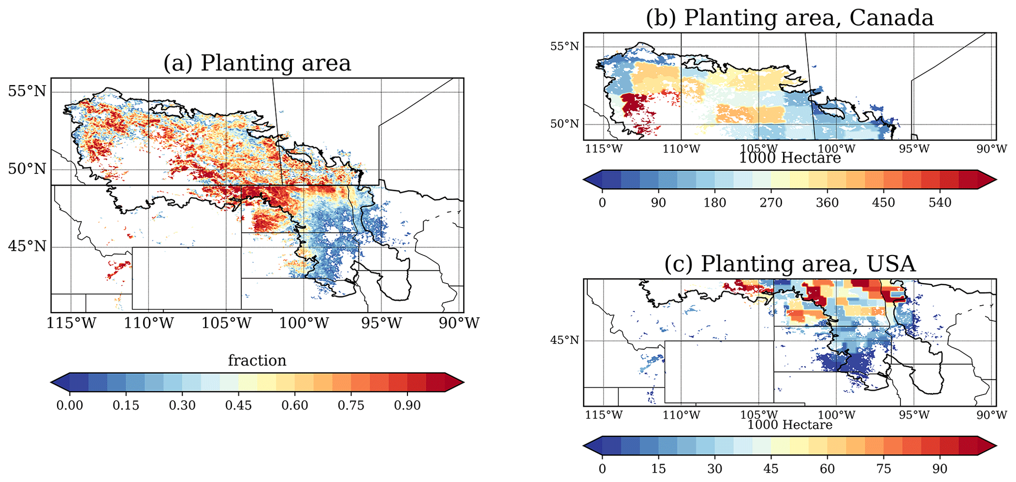
Figure 3Wheat-planting fraction in the study area from the combined dataset from (a) GMU CropScape and AAFC ACI (AAFC Annual Crop Inventory, 2022) and (b) planting area in 1000 ha in the US Northern Great Plains and Canadian Prairies; two color scales are used to accommodate the wide ranges of values from these two data sources.
Yearly spring wheat yield data are collected from USDA NASS and Statistics Canada, which are used for evaluation of the modeled grain biomass. A unit conversion is necessary, considering the standard 15 % of moisture content, from census yield data (bu ac−1, bushels per acre, in the US and kg ha−1 in Canada) to dry grain biomass (g m−2) in model output, according to the test weight conversion charts for Canadian grains (Canada Grain Commission).
To evaluate the wheat leaf phenology, the Moderate Resolution Imaging Spectroradiometer LAI product (MOD15A, Myneni et al., 2015) is used, which provides regional LAI detection at 8 d temporal intervals and 1 km spatial resolution, starting from 2001. This product provides the peak timing and spatial coverage of leaf dynamics within growing seasons, which are useful for evaluating model crop phenology. The 8 d time slices from 1 May to 29 August are selected (16 time slices) to reveal the wheat growing season in this study.
2.6 Experiment design
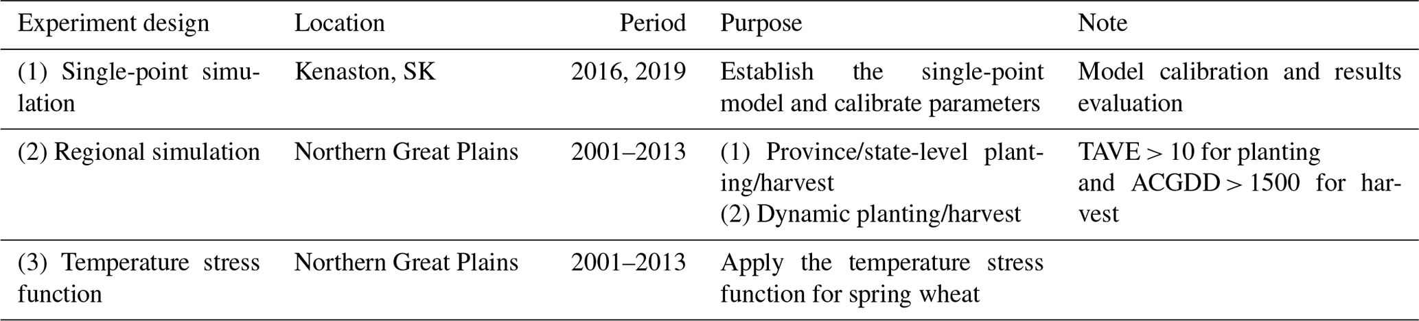
In this study, three individual and progressing experiments are designed. This section provides a brief description of these experiments, and a summary table is presented (Table 1). Rainfed wheat is grown for most of the study region, except for isolated irrigated areas in southern Alberta and central Saskatchewan. Irrigation impacts on crop dynamics and yield will be the focus of future studies.
-
Point-scale simulation. The model is driven by the meteorological forcing collected at the Kenaston site, with prescribed planting and harvest dates. The purpose of this experiment is to obtain a set of wheat-specific parameters against the Kenaston site for 3 available site years of observations. Site observations, including turbulent fluxes (sensible heat (SH) and latent heat (LH)), soil moisture, LAI, and aboveground biomass, are used to evaluate model performance. (See Table A1 in Appendix A for the full details of spring wheat growth parameters used in this study.)
Regional simulations. To facilitate regional simulations, the meteorological forcing data were from the convection-permitting downscale WRF model simulation in the contiguous US (CONUS) and southern Canada (Liu et al., 2017), spanning from 2000 to 2013. The advantages of this dataset are that the high-resolution grid spacing (4 km) provides detailed representation of the heterogeneous surface properties and it allows direction simulation of convective precipitation without using parameterization schemes, both of which are important to agricultural study (Prein et al., 2016; Li et al., 2019). The CONUS dataset has been widely used to study regional climate (Prein et al., 2016; Zhang et al., 2018) and hydrology (Zhang et al., 2020a) in North America.
Two regional planting and harvest simulations are conducted using (1) the province/state-level map for the most typical planting/harvest dates in Canada and US (USDA NASS, 2010) or (2) dynamic dates for planting and harvest based on temperature in the growing season. These two simulations are compared to reflect dynamic agricultural management and interannual weather variability.
Temperature stress function simulation. The purpose of the third simulation is to test the wheat response to high temperature and to demonstrate its variation among regional and interannual scales. This is done by replacing the default function from Eq. (6), Collatz et al. (1991), with a more realistic temperature stress function (Eq. 7) from Wang et al. (2017) (Fig. 2b).
Table 1Experimental design for three sets of crop model simulations.
3.1 Point-scale simulation
Figure 4 shows the growing season GDD, LAI, and aboveground biomass from the field observations and model results as compared to the default (MODIS monthly climatology LAI) results. The growing-stage GDD parameters used in the new wheat model are adopted from a reference paper by Saiyed et al. (2009) for wheat growing in the Canadian Prairies, and the carbon allocation parameters for each growing stage are adopted from the WOFOST model wheat section (Wit and Boogaard, 2021). These parameters are summarized in Appendix A.
It is obvious that the new wheat model has better LAI dynamics compared to the default MODIS monthly LAI, especially for the timing and peak value of LAI. The wheat growing season can be roughly divided into two stages, the vegetative stage and the reproductive stage (grain filling). These two stages are separated by the time of peak LAI within the growing season, before which most of the assimilated carbon is allocated to leaf mass and after which to grain. Therefore, the grain biomass starts to accumulate after the time of peak LAI, shown as the orange lines.
The Kenaston site only recorded the total aboveground biomass in 2019, without differentiation of biomass into individual plant organs. In the Noah-MP crop, total aboveground biomass includes leaf, stem, and grain and is simulated reasonably well for the two 2019 sites (data for 2016 were missing). The yields for 2019 were 2908 and 1635 kg ha−1 for SW30 and SE13, where the model predicted 405 and 247 g m2, respectively. Therefore, the model provides a higher biomass estimate compared to the site-recorded yield in 2019, and these higher yield estimates are discussed in Sect. 3.3.
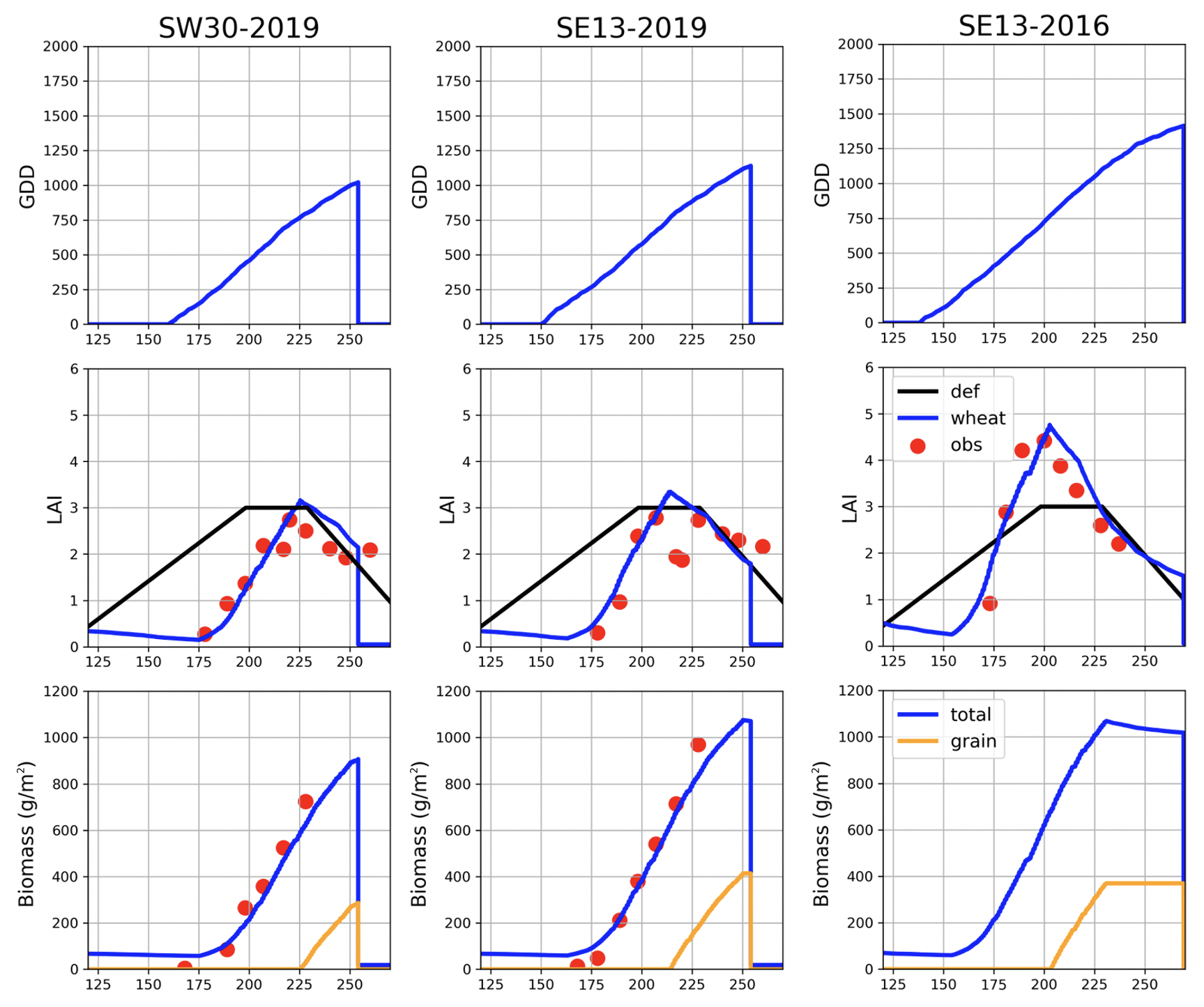
Figure 4Three-site-year growing season GDD, LAI, and aboveground biomass for spring wheat from the field observation and the Noah-MP crop model.
The turbulent fluxes (latent and sensible heat) and soil moisture, as daily time series, for the three growing seasons are provided in Fig. 5. The simulated dynamic LAI from the wheat model presented higher latent heat fluxes compared to default LAI, especially in 3 summer months (JJA). The soil moisture times series show that the Noah-MP crop consumes more soil moisture, especially from the second layer in late growing season since August, as it produces higher latent heat fluxes, suggesting more efficient turbulent exchange of water fluxes between soil and the atmosphere. This has great implications for the vast agricultural regions in the North American Great Plains, as the previous default model may have profoundly underestimated agricultural control of water feedback to regional weather and climate.
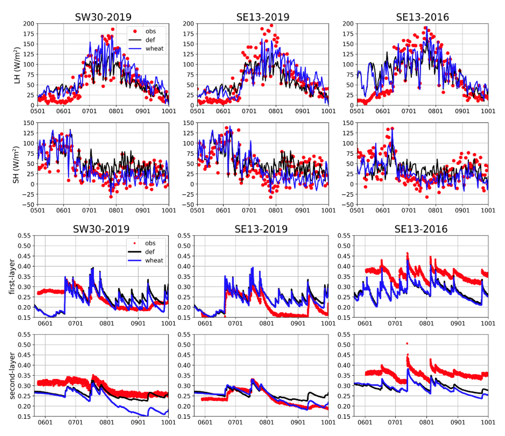
Figure 5Turbulent fluxes (sensible and latent heat, SH and LH) and soil moisture (two layers from 0–10 cm and 10–40 cm) results from the 3-site-year simulation.
The Noah-MP crop model demonstrated reasonable simulations of soil moisture, crop growth, and turbulent fluxes transported to the atmosphere, facilitating the land–atmosphere coupling in croplands on the land surface branch. There is potential for further extending to coupled studies with WRF to assess crop growth's feedback to regional climate.
3.2 Regional dynamics of LAI and yield
Figure 6 shows the spatial distribution of 8 d LAI time slices for the 2007 growing season, 1 May to 29 August (16 slices for 120 d, roughly 4 months), as an example. The time slices show that the regional LAI starts to green up in late May, due to emergence, and reaches its peak around late July, entering the grain-filling stage. After that, the LAI declines until crops mature. Finally, the crops senesce prior to harvest, at which time LAI drops to 0. Spatially, the US portion of the growing region starts emergence and harvest generally earlier than the northwest portion in Canada, and its growing season is shorter – due to warmer average temperatures and faster heat accumulation.
As in the model, the province/state-level planting/harvest uses an arbitrary planting/harvest date for the most usual time windows, regardless of interannual weather variability and spatial heterogeneity within each state. Another obvious deficiency of this approach is the obvious state/province boundaries in LAI values as shown in the figure. Even though two fields might be very closely located geographically, although they are in different states/provinces, they show very different phenology as controlled by the state/province-level planting/harvest season. This is even more so for the crop LAI across US and Canada border. Such province/state-level planting and harvest date treatment leads to the simulated spatial LAI homogenous within but substantially discontinued across a state or province.
The dynamic planting/harvest simulation substantially improves the regional LAI time slices within the growing season. The TAVE threshold triggers planting earlier in the south, as temperature warms up earlier, and the GDD accumulation triggers earlier harvest as well, accounting for the higher/faster heat accumulation. The growing season in the northern region in Canada starts later and also extends longer. Considering these two dynamic thresholds accounts for the south-to-north transition in crop phenology.
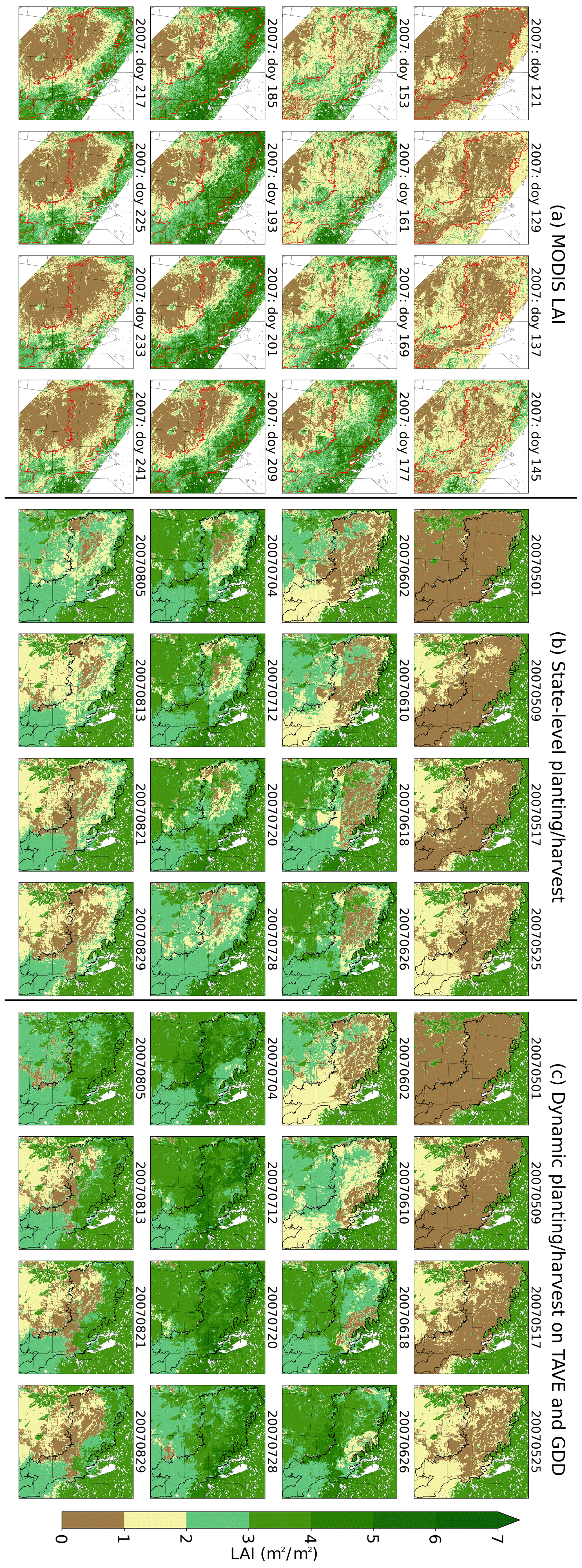
Figure 6Eight-day LAI time slices from (a) MODIS product (MOD15A), (b) province/state-level planting/harvest, and (c) the dynamic planting/harvest simulation.
The large discrepancies between static and dynamic planting/harvest date simulation demonstrate its essential control of growing seasons on accumulated biomass. Figure 7 shows the spatial distribution of yields, planting and harvest date, and the scatter plot between the grain-filling stage duration (days) and the final yield. The province/state-level grain-filling stage durations are much longer than in the dynamic simulation, thus leading to substantially overestimated yields compared to the dynamic planting/harvest simulation and census data. The color scale in the scatter plot indicates the planting date, which also suggests the earlier the planting, the longer the grain-filling stage and hence higher yield.
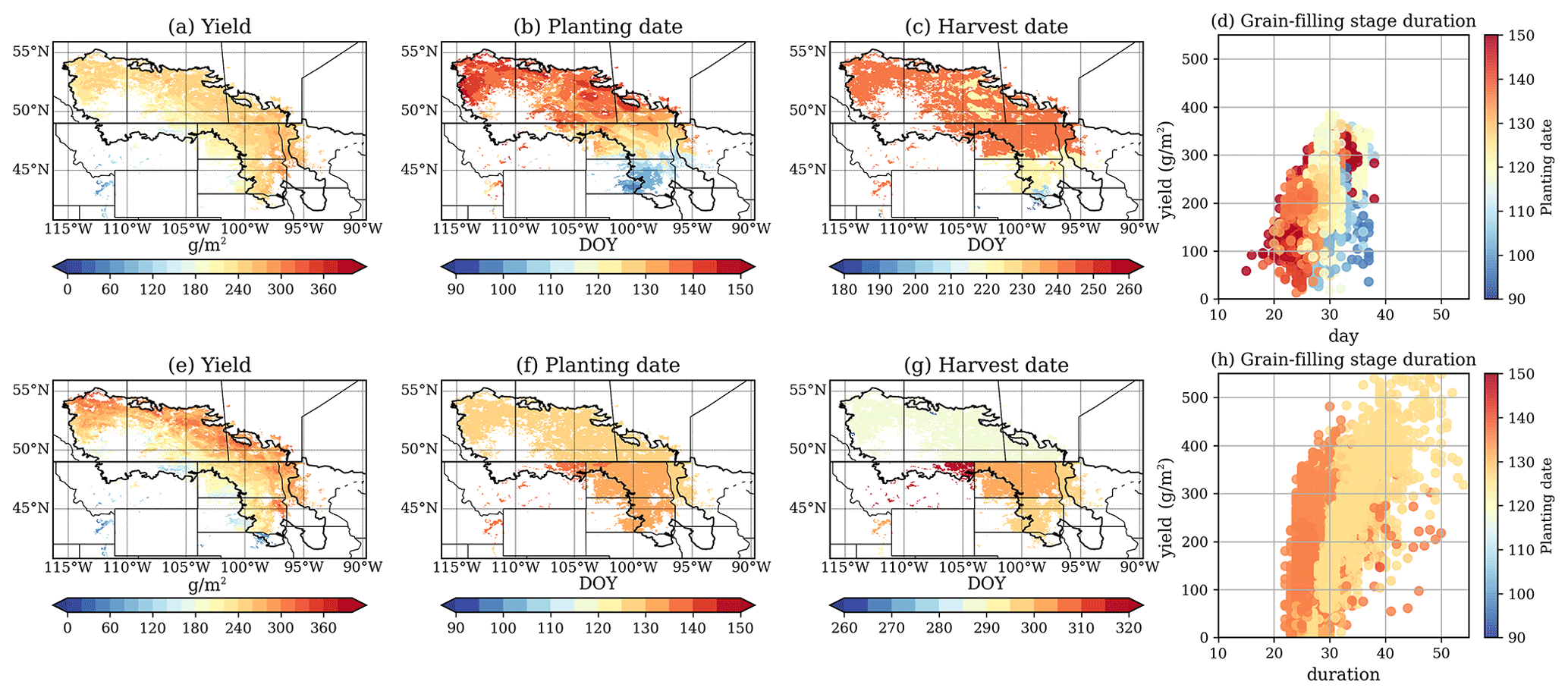
Figure 7Model results of (a) yield, (b) planting date, (c) harvest date, and (d) scatter plot between yield (g m−2, y axis) and duration of the grain-filling stage (day, x axis) from default province/state-level (top) and dynamic (bottom) planting/harvest and dynamic simulation.
3.3 Temperature stress function
Figure 8 presents the spatial difference pattern between two simulations and the census data. The crop yield estimates from the default temperature function show much overestimation, especially in Saskatchewan and North and South Dakota (Fig. 8a). Applying the temperature stress function in Wang et al. (2017) shows an obvious yield reduction around 10 % from default simulations (Fig. 8b), hence improving the crop yield results. The spatial distribution of this reduction is more evident in the southeast domain in North Dakota, Minnesota, and Manitoba, where the average temperature is higher and heat stresses are more likely. The yields in cooler provinces, Alberta and Saskatchewan, are less affected.
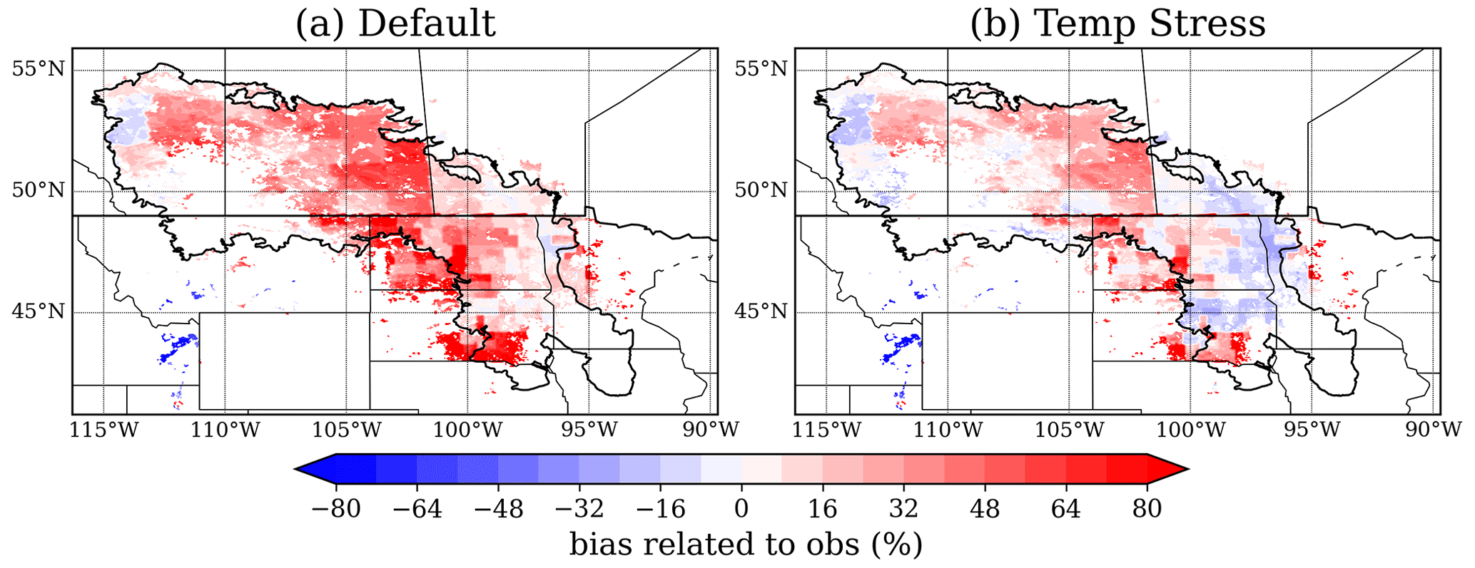
Figure 8Simulated grain yield compared to the census data from Statistics Canada and USDA NASS from the (a) default and (b) the new temperature stress simulation.
The P90 threshold, derived from the 90th percentile of the 30-year daily maximum temperature climatology, can be used to characterize extreme temperatures. When the daily maximum temperature exceeds this threshold, it can be counted as a hot day (Zhang et al., 2011; Perkins and Alexsander, 2013). Counting the number of hot days (NHD) within a growing season is a good indicator for the frequency of extreme heat events (Zhang et al., 2011, 2018). Figure 9 below shows the scatter plot relationship between the NHD within the growing season (May to September) and final yield in three Canadian Prairie Provinces.
Although presumably negative impacts of high-temperature stress on wheat yield are expected, discrepancies among these three provinces are obvious in both census data and model results. For Alberta (AB) and Saskatchewan (SK), the negative impacts of extreme hot days on grain biomass are most evident, and the model has captured this relationship reasonably well, suggesting that the temperature stress plays a profound role in final crop yield. The temperature stress simulation shows a further reduction on the final yield, especially with higher NHD, which contributes to less overestimated biases (about 10 % reduction) compared to the default configuration.
For Manitoba (MB), the higher quantile yield decreases with NHD, while the lower quantile yields actually increase amid higher NHD. These two distinct features suggest that temperature stress is not the only factor limiting the final yield in this province. In some part of MB summertime precipitation is significantly higher than that in AB and SK, so that low NHD may suggest more precipitation and low exposure to sunlight, which in turns limits the photosynthesis and biomass accumulation. In other words, the wheat productivity in MB is less water limited than that in AB and SK. The Noah-MP crop model adequately captures these two distinct responses to NHD conditions. Additionally, the temperature stress modification limits the final yield reduction to 10 % as well.
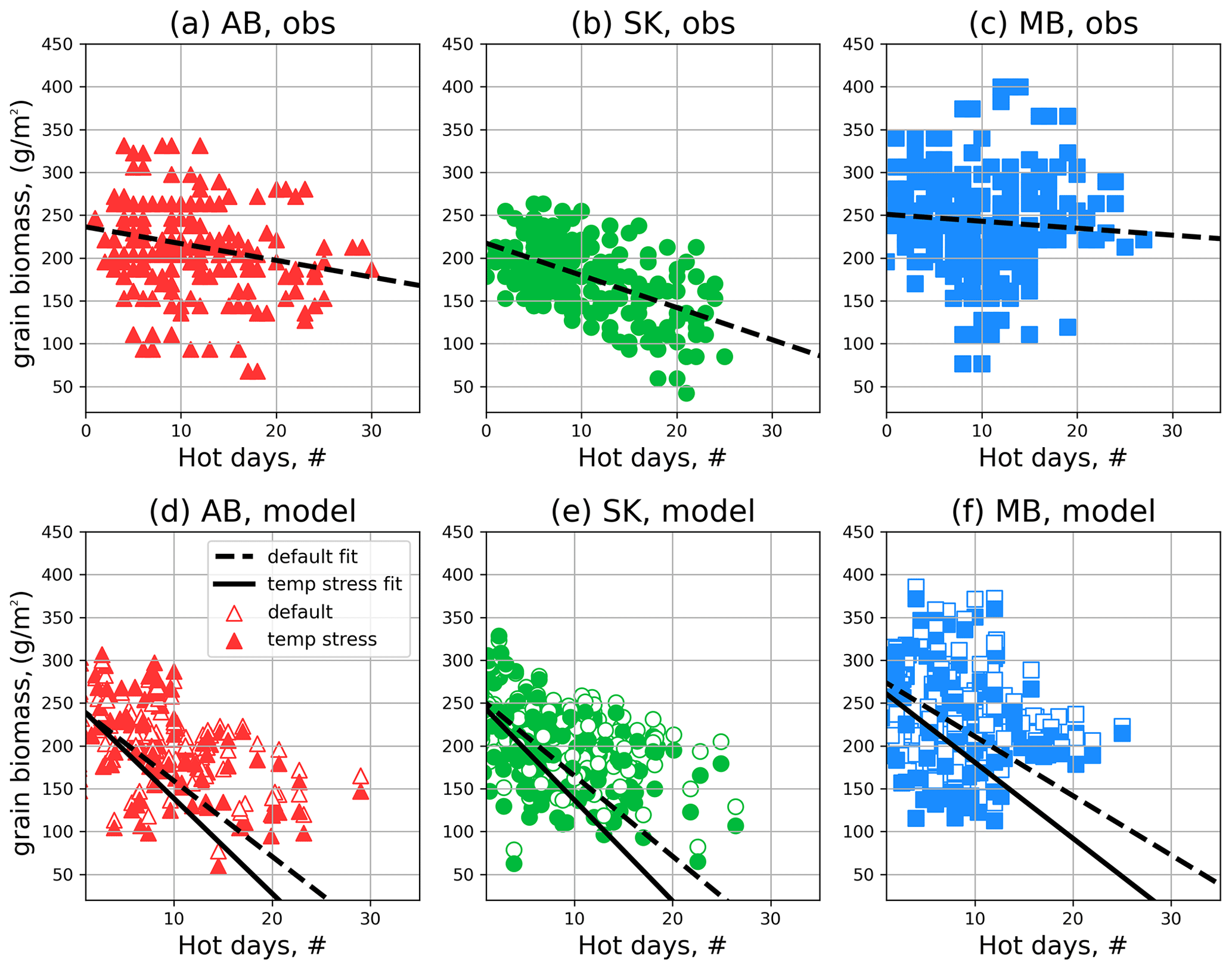
Figure 9Scatter plot of NHD (x axis) vs. yield (y axis) at three Canadian Provinces, from Statistics Canada (a–c) and model results (d–f).
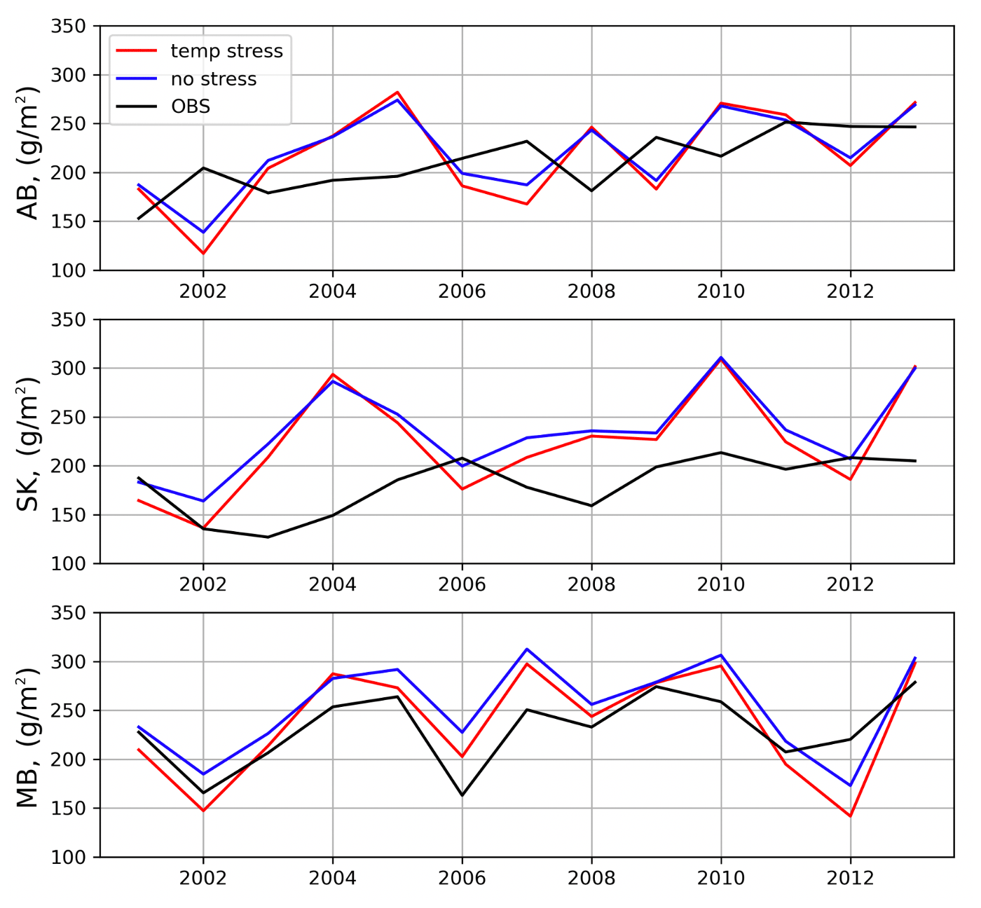
From 2001 to 2013, an increasing trend of yield is apparent in each province, from both census data and model simulations (Fig. 10). In addition, strong interannual variability exists in these trends, and the model's performance varies in each province. For MB, the model produces the best results in terms of trend and interannual variability. The temperature stress simulation further produces stressed yield results corresponding to heatwave events in 2002 and 2006, which largely agrees with the observations. As for 2012, both the default simulation and the temperature stress simulation underestimate the crop yields, which suggests there might be other factors missing in the simulation.
However, as for SK and AB, to capture the interannual variability is challenging, especially in AB, where the model shows a high yield peak while the census data show a lower value. A possible speculation for this discrepancy would be that there are larger extents of irrigated croplands in AB than in other provinces and thus have less water limitation in those warmer years. Presumably, these irrigated high yields could bias the observed Statistics Canada yield, i.e., yield not connected to environmental conditions that the model is limited to. This suggests that although the model presents reasonable estimates of mean yield results, it is very difficult to capture interannual variability, due to the weather variations within each growing season. Applying irrigation in Noah-MP crop could potentially improve the crop yield simulated in AB, yet we currently lack the spatial distribution and irrigation amount data. These data are essential to improve our understanding of crop yield responses to heat and water stress and the model performance to reasonably capture such responses.
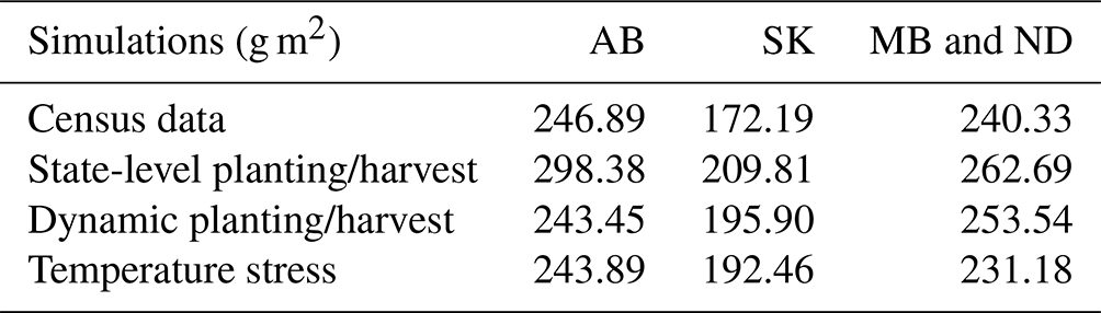
The statistics of yield from the census data and various simulations are presented in Table 2. As compared to the census data, the province/state-level simulation shows the highest yield among all simulations due to unadjusted growing season length and higher optimal temperature. The dynamic planting/harvest substantially restricts the yield in the northern part of the domain, as the province/state-level planting/harvest fails to represent the growing season dynamics in this region. Finally, the temperature stress function cuts about 10 % of the yield in Manitoba and North Dakota, while it has little effect in AB, where temperature stress is not as strong as other provinces.
Table 2Summary of the yield for different simulations over three regions. ND represents North Dakota.
4.1 Discrepancies in using MODIS to evaluate growing season phenology
The MODIS 8 d LAI product provides the first remote sensing comparison for regional-scale modeled LAI for spring wheat in the Northern Great Plains. However, large uncertainties remain over its inadequacy in detecting different crop species and spatial resolution in representing the heterogeneity at field scales. For example, there are three major crop types in Saskatchewan: cereals (mainly wheat and some barley), pulses (chickpea, lentils), and canola. However, with crop rotation between these types at scales within the MODIS LAI product, we cannot differentiate the LAI for specific crop types. For example, with a point-to-pixel comparison of the LAI time series from the Kenaston site with the MODIS LAI, higher values are shown from MODIS data, which could be related to canola in surrounding fields.
On the other hand, the original annual crop inventory data from AAFC and CropScape (at 30 m) only represents the temporal frequency of these crops – however, it is often used as spatial fraction. It may be the case that for some places wheat may be frequently planted but not at significant extent compared to other crops types in the region. For the US portion, corn and soybeans are also popularly planted in the Red River valley between Minnesota and North Dakota.
Due to the reasons above, previous regional crop model simulations reliant on large-scale LAI remote sensing products in North America have challenges in modeling crop-specific phenology and LAI dynamics. Thus, one should consider products like the MODIS LAI valuable to assess the qualitative evolution of LAI in growing seasons, while quantitative comparisons should be treated with caution and with an expectation of bias that relates to the relative extent of the crop type of interest in the local crop rotation.
4.2 Uncertainty in planting and harvest date
This study attempts to adopt the dynamic planting/harvest date as a more advanced approach to the province/state-level date. Yet there are much more complex dimensions involved in practice in reality. An aspect not captured by temperature/GDD thresholding is that there are differences in day length (and therefore incident shortwave radiation that drives photosynthesis/photoperiods) across this range in latitude that do moderate some of the GDD differences. Some crop models have already considered characterizing the day length (Setiyono et al., 2007) and can become common practice in an also integrated ESM crop model approach.
In the Canadian Prairies, the major restriction for planting and harvest is temperature, usually planting from late April to early May after sufficient time since snowfall and melting while harvesting from late August to early September to avoid the first frost in fall.
Agronomic and logistical considerations determine the actual planting and harvesting dates to accommodate reality and non-optimal conditions. In cool/wet springs planting operations will be delayed until fields are dry enough to allow machine access, and seed placement will be shallow to take advantage of near-surface soil moisture and facilitate faster emergence. In contrast, in warm–dry conditions, planting will occur earlier with deeper seed placement to increase germination potential and to limit the period of soil evaporation losses and maximize crop water use efficiency. Harvest operations can also be disconnected from physiological maturity as storage implications of grain moisture are critical to avoid post-harvest losses. Except for early frost events, prior to maturity, quality losses after senescence are limited and so timing of harvest operations is determined by the interactions between grain moisture and precipitation and humidity conditions. Then comes a critical question: given that farmers keep planting/harvest in a quite stable time period while the year-to-year weather is fluctuating, should these in-depth wisdoms be incorporated into the modeling process or not? This question is still remains uncertain and unanswered in current stage of crop model research.
4.3 Temperature stress function
In current crop models, heat stress impacts on crop growth and final yield in two ways: (1) the temperature stress function is applied in the photosynthesis–stomata subroutine, with high temperature regulating/limiting the plant physiological function; (2) heat accumulation, calculated as GDD, is utilized to advance into various growing stages, defined by GDD thresholds. Higher temperatures accelerate heat accumulation and result in shorter phenological developments, which ultimately lead to lower crop yield. Multiple studies have been dedicated to address the first way – heat stress impacts on crop photosynthesis behaviors (Bernacchi et al., 2013; Siebert et al., 2014; Levis, 2014). Siebert et al. (2014) claimed there is a substantial difference between applying air temperature and canopy temperature in crop model studies during heatwaves – the latter can be 7 ∘C warmer than the former, depending on soil moisture. This highlights one of the advantages of integrated ESM- or LSM-based crop models, such as the Noah-MP crop model, for using canopy temperature, calculated from energy balance, rather than air temperature for photosynthesis process.
Moreover, high-temperature stress has co-occurred along with water stress – rising temperature increases evaporation demand, depleting soil moisture with dry conditions – and leads to a compound heat–water stress (Lesk et al., 2022). As a result, previous large-scale statistical studies (Lobell et al., 2011b) have revealed crop yield decline corresponding to temperature warmer than 30 ∘C, which is 5–10 ∘C lower than plant-scale studies (Prasad et al., 2011). In our study, the new temperature stress function adopted from Wang et al. (2017) has shown a lower temperature for optimal photosynthesis compared to the function developed from Collatz et al. (1991) from lab measurements (35 ∘C). Judging from the simulated results, the new temperature stress function has better performance and less overestimation. To obtain a comprehensive understanding of temperature stress on crop yield, we still call for potential applications of ESM-based crop models in the future, as temperature and moisture processes are better integrated within model structures.
For the second way, there have been debates on the use of fixed GDD thresholds for regulating growing stages, especially between crop model developers and genotype seed breeders. For example, crop modelers tend to use the GDD-based thresholds to constrain and regulate crop growing seasons while these thresholds are artificial and empirical (based on the site where the model is developed and is subject to parameter calibration). Recent advances through seed breeding and genetically modified organisms (GMOs) have provided new crop genotypes every 2–3 years, which has been a fundamental reason for a continuous increasing trend in crop yield in the last half century – for example, the International Maize and Wheat Improvement Center (CIMMYT) has recently made efforts to breed early-maturing and heat-tolerant wheat varieties, aiming to adapt wheat lines from South Asia to the conditions in Mexico (Mondal et al., 2016).
This brings in a paradoxical situation that crop modelers, agroclimatic scientists, agronomists, and farmers are relying on statics empirical GDD thresholds to estimate crop growth when these thresholds are in fact dynamic. So is there any value in using static GDD thresholds of current crops to predict future crop yield under climate change when forthcoming advances in genotypes will almost surely break through such thresholds?
There is no simple yes or no answer to the question above. Nonetheless, such questions manifest themselves through the progress of model parameterization. Most crop modeling schemes that are capable of coupling crop–climate interactions such as Noah-MP still require GDD-based approaches to characterize crop growth. Higher-order representations that consider gene effects on phenology directly exist, but their complexity makes simulating the entire genetic controls on specific traits impossible (Wang et al., 2019). In this context, it is critical to understand the GDD threshold approach limitations and consider approaches to capture the evolving GDD threshold dynamics.
Spring wheat production in the Canadian Prairies and US Northern Great Plains is a significant source of wheat for domestic food supply and international exports. This study establishes an example for the development of a new crop species within the Noah-MP crop model framework and its application in large regional simulations. The study further investigates the crop model responses to heat stress within a 13-year study period. We found the following.
-
The point-scale spring crop model successfully captures spring wheat LAI dynamics for 3 site years in Kenaston, SK, Canada, compared with default monthly climatology LAI. The simulated higher LAI results in more efficient water movement from the soil to the atmosphere, mediated by plants' stomata. Therefore, this single-point model demonstrates the ability to quantify the vertical continuum of the complex energy–water–carbon exchange within the atmosphere–crop–soil system.
-
To propagate the point-scale crop model to the regional scale, dynamic planting/harvest triggers are applied to better depict the heterogenous farming practices than a province/state-level map used in a previous study. This approach not only improves the growing season LAI, as evaluated by MODIS 8 d LAI time slices, but also the final yield, compared to agricultural census data. It is also shown that the modeled yield is closely related to the duration of crops' grain-filling stage, highlighting the importance of reasonably capturing the spring wheat phenology. It is noted that the improved results obtained in this study through dynamic planting/harvest are for the spring wheat planted in the Northern Great Plains and Canadian Prairies. As a general approach to capture the spatiotemporal heterogeneity for the planting dynamics, future studies are encouraged to a larger region or global crop model applications.
-
An updated temperature response function is implemented within the photosynthesis–stomata process in the crop model to better represent the optimal temperature range for wheat growing conditions. This simulation shows reduced final yield by about 10 % in southern states in the US and Manitoba in Canada, while it does not have a significant effect in Alberta. The interannual variability of crop yields is well captured for Manitoba, especially for the yield damages due to heatwaves in the recent decade.
Finally, the model results are discussed in various aspects, including limitations in uncertain planting/harvest dates and the heat stress function, as well as potential future development. The model's capability to reasonably simulate interannual variability and the large spatial distribution of growing season LAI and final yields was demonstrated.
This work has great implications for developing the methods to address how crop production will be affected by future climate change, warmer temperatures, and uncertain precipitation patterns, which are critical to future research be the next step in our research.
Table A1Spring wheat parameters in the Noah-MP crop model in this study.
The Noah-MP model is driven by the National Center for Atmospheric Research (NCAR) high-resolution land data assimilation system (Chen et al., 2007) and can be downloaded from https://github.com/CharlesZheZhang/hrldas/tree/wheat (last access: December 2022) (access https://doi.org/10.5281/zenodo.7556048, Cenlin_He et al., 2023a). The Noah-MP LSM can be accessed from https://github.com/CharlesZheZhang/noahmp/tree/wheat (last access: December 2022) with the release of the code (v4.4 with spring wheat dynamics with DOI https://doi.org/10.5281/zenodo.7556046, Cenlin_He et al., 2023b).
The modeling results and analysis data used in this study are uploaded to and can be accessed through the Zenodo repository: https://doi.org/10.5281/zenodo.7023831 (Zhang, 2022).
The regional-scale crop planting area data are available from the USDA NASS website (https://nassgeodata.gmu.edu/CropScape/, Han et al., 2012). The county-level crop yield data are available from the USDA NASS website (https://quickstats.nass.usda.gov/ (U.S. NASS, 2022).
The census agricultural region data can be downloaded from the Statistics Canada website (https://doi.org/10.25318/3210000201-eng, Statistics Canada, 2022).
The 13-year forcing data for regional simulations are from the CONUS WRF simulation and can be accessed at https://rda.ucar.edu/datasets/ds612.0 (last access: December 2022) (https://doi.org/10.5065/D6V40SXP, Rasmussen and Liu, 2017).
The supplement related to this article is available online at: https://doi.org/10.5194/gmd-16-3809-2023-supplement.
ZZ, YL, and FC conceptualized the study and ZZ performed the simulations. ZZ and FC designed the methodology, developed the model code, and updated the model parameters. PH and WH provided the observational data resources for model validation. ZZ prepared the original draft of the manuscript with reviewing and editing from all co-authors. YL and FC provided valuable advice and supervision throughout the whole process.
The contact author has declared that none of the authors has any competing interests.
Any
opinions, findings, conclusions or recommendations expressed in this
publication are those of the authors and do not necessarily reflect the
views of the National Science Foundation.
Publisher's note: Copernicus Publications remains neutral with regard to jurisdictional claims in published maps and institutional affiliations.
Zhe Zhang, Yanping Li, Phillip Harder, Warren Helgason, James Famiglietti, and Zhenua Li acknowledge the support of the Global Institute for Water Security and the Global Water Futures program by the Canada First Research Excellence Fund. Fei Chen, Prasanth Valayamkunnath, and Cenlin He acknowledge the support of the National Center for Atmospheric Research, Water System Program, USDA NIFA grant 2015-67003-23460, NSF INFEWS grant 1739705, and NOAA OAR grant NA18OAR4590381. NCAR is sponsored by the National Science Foundation.
This research has been supported by the Global Institute for Water Security, University of Saskatchewan (Agricultural Water Futures grant); the Global Water Futures (Agricultural Water Futures grant); the National Institute of Food and Agriculture (grant no. 2015-67003-23460); the National Science Foundation (grant no. 1739705); and the National Oceanic and Atmospheric Administration (grant no. NA18OAR4590381).
This paper was edited by Sam Rabin and reviewed by Jyoti Singh and one anonymous referee.
Agyeman, R. Y. K., Huo, F., Li, Z., and Li, Y.: Modelled changes in selected agroclimatic indices over the croplands of western Canada under the RCP8.5 scenario, Q. J. Roy. Meteor. Soc., 147, 4454–4467, https://doi.org/10.1002/qj.4188, 2021.
Annual Crop Inventory: Agriculture and Agri-Food Canada, https://www.agr.gc.ca/atlas/apps/metrics/index-en.html?appid=aci-iac; last access: October 2022.
Bernacchi, C. J., Bagley, J. E., Serbin, S. P., Ruiz-Vera, U. M., Rosenthal, D. M., and Vanloocke, A.: Modelling C3 photosynthesis from the chloroplast to the ecosystem, Plant. Cell Environ., 36, 1641–1657, https://doi.org/10.1111/pce.12118, 2013.
Carew, R., Meng, T., Florkowski, W. J., Smith, R., and Blair, D.: Climate change impacts on hard red spring wheat yield and production risk: evidence from Manitoba, Canada, Can. J. Plant Sci., 98, 782–795, https://doi.org/10.1139/cjps-2017-0135, 2017.
Cenlin_He, Barlage, M., xutr-bnu, Zhang, Z., Mocko, D., and Chen, F.: CharlesZheZhang/hrldas: HRLDAS driver for NoahMP LSM v4.4 with spring wheat (v4.4), Zenodo [code], https://doi.org/10.5281/zenodo.7556048, 2023a.
Cenlin_He, Barlage, M., Valayamkunnath, P., Gill, D., Mocko, D., and Chen, F.: CharlesZheZhang/noahmp: NoahMP LSM v4.4 with spring wheat (v4.4), Zenodo [code], https://doi.org/10.5281/zenodo.7556046, 2023b.
Chen, F., Manning, K. W., Lemone, M. A., Trier, S. B., Alfieri, J. G., Roberts, R., Tewari, M., Niyogi, D., Horst, T. W., Oncley, S. P., Basara, J. B., and Blanken, P. D.: Description and evaluation of the characteristics of the NCAR high-resolution land data assimilation system, J. Appl. Meteorol. Clim., 46, 694–713, https://doi.org/10.1175/JAM2463.1, 2007.
Collatz, G. J., Ball, J. T., Grivet, C., and Berry, J. A.: Physiological and environmental regulation of stomatal conductance, photosynthesis and transpiration: a model that includes a laminar boundary layer, Agr. Forest Meteorol., 54, 107–136, https://doi.org/10.1016/0168-1923(91)90002-8, 1991.
CropScape, USDA NASS and GMU: https://nassgeodata.gmu.edu/CropScape/, last access: October 2022.
De Wit, A. and Boogaard, H.: A gentle introduction to WOFOST, in: Wageningen Environmental Research, November, https://www.wur.nl/en/research-results/research-institutes/environmental-research/facilities-tools/software-models-and-databases/wofost/documentation-wofost.htm (last access: October 2022), 2021.
ERS USDA wheat: https://www.ers.usda.gov/topics/crops/wheat/wheat-sector-at-a-glance/, last access: October 2022.
Han, W., Yang, Z., Di, L., and Mueller, R.: CropScape: A Web service based application for exploring and disseminating US conterminous geospatial cropland data products for decision support, Comput. Electron. Agr., 84, 111–123, https://doi.org/10.1016/j.compag.2012.03.005, 2012.
Harley, P. C. and Tenhunen, J. D.: Modeling the Photosynthetic Response of C3 Leaves to Environmental Factors, in Modeling Crop Photosynthesis – from Biochemistry to Canopy, 17–39, https://doi.org/10.2135/cssaspecpub19.c2, 1991.
Iizumi, T., Kim, W., and Nishimori, M.: Modeling the Global Sowing and Harvesting Windows of Major Crops Around the Year 2000, J. Adv. Model. Earth Sy., 11, 99–112, 2018.
IPCC: Climate change 2014: synthesis report Contribution of Working Groups I, II and III to the Fifth Assessment Report of the Intergovernmental Panel on Climate Change, edited by: Pachauri, R. K. and Meyer, L. A., Geneva, IPCC, 151 pp., 2014.
Jägermeyr, J., Müller, C., Ruane, A. C., Elliott, J., Balkovic, J., Castillo, O., Faye, B., Foster, I., Folberth, C., Franke, J. A., Fuchs, K., Guarin, J. R., Heinke, J., Hoogenboom, G., Iizumi, T., Jain, A. K., Kelly, D., Khabarov, N., Lange, S., Lin, T.-S., Liu, W., Mialyk, O., Minoli, S., Moyer, E. J., Okada, M., Phillips, M., Porter, C., Rabin, S. S., Scheer, C., Schneider, J. M., Schyns, J. F., Skalsky, R., Smerald, A., Stella, T., Stephens, H., Webber, H., Zabel, F., and Rosenzweig, C.: Climate impacts on global agriculture emerge earlier in new generation of climate and crop models, Nat. Food, 2, 873–885, https://doi.org/10.1038/s43016-021-00400-y, 2021.
Lesk, C., Anderson, W., Rigden, A., Coast, O., Jägermeyr, J., McDermid, S., Davis, K. F. and Konar, M.: Compound heat and moisture extreme impacts on global crop yields under climate change, Nat. Rev. Earth Environ., 3, 872–889, https://doi.org/10.1038/s43017-022-00368-8, 2022.
Levis, S.: Crop heat stress in the context of Earth System modeling, Environ. Res. Lett., 9, 061002, https://doi.org/10.1088/1748-9326/9/6/061002, 2014.
Li, Y., Li, Z., Zhang, Z., Chen, L., Kurkute, S., Scaff, L., and Pan, X.: High-resolution regional climate modeling and projection over western Canada using a weather research forecasting model with a pseudo-global warming approach, Hydrol. Earth Syst. Sci., 23, 4635–4659, https://doi.org/10.5194/hess-23-4635-2019, 2019.
Liu, C., Ikeda, K., Rasmussen, R., Barlage, M., Newman, A. J., Prein, A. F., Chen, F., Chen, L., Clark, M., Dai, A., Dudhia, J., Eidhammer, T., Gochis, D., Gutmann, E., Kurkute, S., Li, Y., Thompson, G., and Yates, D.: Continental-scale convection-permitting modeling of the current and future climate of North America, Clim. Dynam., 49, 71–95, https://doi.org/10.1007/s00382-016-3327-9, 2017.
Liu, X., Chen, F., Barlage, M., Zhou, G., and Niyogi, D.: Noah-MP-Crop: Introducing dynamic crop growth in the Noah-MP land surface model, J. Geophys. Res.-Atmos., 121, 13953–13972, https://doi.org/10.1002/2016JD025597, 2016.
Lobell, D. B., Schlenker, W., and Costa-Roberts, J.: Climate Trends and Global Crop Production Since 1980, Science, 80, 616–620, https://doi.org/10.1126/science.1204531, 2011a.
Lobell, D. B., Bänziger, M., Magorokosho, C., and Vivek, B.: Nonlinear heat effects on African maize as evidenced by historical yield trials, Nat. Clim. Change, 1, 42–45, https://doi.org/10.1038/nclimate1043, 2011b.
McDermid, S. S., Mearns, L. O., and Ruane, A. C.: Representing agriculture in Earth System Models: Approaches and priorities for development, J. Adv. Model. Earth Sy., 9, 2230–2265, https://doi.org/10.1002/2016MS000749, 2017.
Mondal, S., Singh, R. P., Mason, E. R., Huerta-Espino, J., Autrique, E., and Joshi, A. K.: Grain yield, adaptation and progress in breeding for early-maturing and heat-tolerant wheat lines in South Asia, F. Crop. Res., 192, 78–85, https://doi.org/10.1016/j.fcr.2016.04.017, 2016.
Myneni, R., Knyazikhin, Y., and Park, T.: MOD15A2H MODIS/Terra Leaf Area Index/FPAR 8-Day L4 Global 500m SIN Grid V006, NASA EOSDIS Land Processes DAAC [data set], https://doi.org/10.5067/MODIS/MOD15A2H.006, 2015.
Niu, G.-Y., Yang, Z.-L., Mitchell, K. E., Chen, F., Ek, M. B., Barlage, M., Kumar, A., Manning, K., Niyogi, D., Rosero, E., Tewari, M., and Xia, Y.: The community Noah land surface model with multiparameterization options (Noah-MP): 1. Model description and evaluation with local-scale measurements, J. Geophys. Res., 116, D12109, https://doi.org/10.1029/2010JD015139, 2011.
Perkins, S. E. and Alexander, L. V.: On the measurement of heat waves, J. Climate, 26, 4500–4517, https://doi.org/10.1175/JCLI-D-12-00383.1, 2013.
Prasad, P. V. V., Pisipati, S. R., Momčilović, I., and Ristic, Z.: Independent and Combined Effects of High Temperature and Drought Stress During Grain Filling on Plant Yield and Chloroplast EF-Tu Expression in Spring Wheat, J. Agron. Crop Sci., 197, 430–441, https://doi.org/10.1111/j.1439-037X.2011.00477.x, 2011.
Prein, A. F., Rasmussen, R. M., Ikeda, K., Liu, C., Clark, M. P., and Holland, G. J.: The future intensification of hourly precipitation extremes, Nat. Clim. Change, 7, 48–52, https://doi.org/10.1038/nclimate3168, 2016.
Qian, B., De Jong, R., Warren, R., Chipanshi, A., and Hill, H.: Statistical spring wheat yield forecasting for the Canadian prairie provinces, Agr. Forest Meteorol., 149, 1022–1031, https://doi.org/10.1016/j.agrformet.2008.12.006, 2009.
Qian, B., Zhang, X., Smith, W., Grant, B., Jing, Q., Cannon, A. J., Neilsen, D., McConkey, B., Li, G., Bonsal, B., Wan, H., Xue, L. and Zhao, J.: Climate change impacts on Canadian yields of spring wheat, canola and maize for global warming levels of 1.5 ∘C, 2.0 ∘C, 2.5 ∘C and 3.0 ∘C, Environ. Res. Lett., 14, 074005, https://doi.org/10.1088/1748-9326/ab17fb, 2019.
Rasmussen, R. and Liu, C.: High Resolution WRF Simulations of the Current and Future Climate of North America, Research Data Archive at the National Center for Atmospheric Research, Computational and Information Systems Laboratory [data set], https://doi.org/10.5065/D6V40SXP, 2017.
Rosenzweig, C., Jones, J. W., Hatfield, J. L., Ruane, A. C., Boote, K. J., Thorburn, P., Antle, J. M., Nelson, G. C., Porter, C., Janssen, S., Asseng, S., Basso, B., Ewert, F., Wallach, D., Baigorria, G., and Winter, J. M.: The Agricultural Model Intercomparison and Improvement Project (AgMIP): Protocols and pilot studies, Agr. Forest Meteorol., 170, 166–182, https://doi.org/10.1016/j.agrformet.2012.09.011, 2013.
Sacks, W. J., Deryng, D., Foley, J. A., and Ramankutty, N.: Crop planting dates: an analysis of global patterns, Global Ecol. Biogeogr., 19, 607–620, https://doi.org/10.1111/j.1466-8238.2010.00551.x, 2010.
Saiyed, I. M., Bullock, P. R., Sapirstein, H. D., Finlay, G. J., and Jarvis, C. K.: Thermal time models for estimating wheat phenological development and weather-based relationships to wheat quality, Can. J. Plant Sci., 89, 429–439, https://doi.org/10.4141/CJPS07114, 2009.
Semenov, M. A. and Shewry, P. R.: Modelling predicts that heat stress, not drought, will increase vulnerability of wheat in Europe, Sci. Rep., 1, 66, https://doi.org/10.1038/srep00066, 2011.
Setiyono, T. D., Weiss, A., Specht, J., Bastidas, A. M., Cassman, K. G., and Dobermann, A.: Understanding and modeling the effect of temperature and daylength on soybean phenology under high-yield conditions, F. Crop. Res., 100, 257–271, https://doi.org/10.1016/j.fcr.2006.07.011, 2007.
Siebert, S., Ewert, F., Eyshi Rezaei, E., Kage, H., and Graß, R.: Impact of heat stress on crop yield – On the importance of considering canopy temperature, Environ. Res. Lett., 9, 044012, https://doi.org/10.1088/1748-9326/9/4/044012, 2014.
Skamarock, W., Klemp, J., Dudhia, J., Gill, D., Barker, M., Duda, M., Huang, X.-Y., Wang, W., and Powers, J.: A Description of the Advanced Research WRF Version 3, (No. NCAR/TN-475+STR), University Corporation for Atmospheric Research, https://doi.org/10.5065/D68S4MVH, 2008.
Statistics Canada: Table 32-10-0002-01 Estimated areas, yield and production of principal field crops by Small Area Data Regions, in metric and imperial units, https://doi.org/10.25318/3210000201-eng, web archive: https://www150.statcan.gc.ca/t1/tbl1/en/tv.action?pid=3210000201, last access: October 2022.
United States U.S. National Agricultural Statistics Service NASS (US NASS): Web archive, https://quickstats.nass.usda.gov/, last access: October 2022.
USDA NASS: Economics, Statistics and Market Information System, Usual Planting and Harvesting Dates for US Field Crops, https://usda.library.cornell.edu/concern/publications/vm40xr56k (last access: October 2022), 2010.
Wang, E., Martre, P., Zhao, Z., Ewert, F., Maiorano, A., Rötter, R. P., Kimball, B. A., Ottman, M. J., Wall, G. W., White, J. W., Reynolds, M. P., Alderman, P. D., Aggarwal, P. K., Anothai, J., Basso, B., Biernath, C., Cammarano, D., Challinor, A. J., De Sanctis, G., Doltra, J., Fereres, E., Garcia-Vila, M., Gayler, S., Hoogenboom, G., Hunt, L. A., Izaurralde, R. C., Jabloun, M., Jones, C. D., Kersebaum, K. C., Koehler, A. K., Liu, L., Müller, C., Naresh Kumar, S., Nendel, C., O'Leary, G., Olesen, J. E., Palosuo, T., Priesack, E., Eyshi Rezaei, E., Ripoche, D., Ruane, A. C., Semenov, M. A., Shcherbak, I., Stöckle, C., Stratonovitch, P., Streck, T., Supit, I., Tao, F., Thorburn, P., Waha, K., Wallach, D., Wang, Z., Wolf, J., Zhu, Y., and Asseng, S.: The uncertainty of crop yield projections is reduced by improved temperature response functions, Nat. Plants, 3, 17102, https://doi.org/10.1038/nplants.2017.102, 2017.
Wang, E., Brown, H. E., Rebetzke, G. J., Zhao, Z., Zheng, B., and Chapman, S. C.: Improving process-based crop models to better capture genotype × environment × management interactions, J. Exp. Bot., 70, 2389–2401, https://doi.org/10.1093/jxb/erz092, 2019.
Wutzler, T., Lucas-Moffat, A., Migliavacca, M., Knauer, J., Sickel, K., Šigut, L., Menzer, O., and Reichstein, M.: Basic and extensible post-processing of eddy covariance flux data with REddyProc, Biogeosciences, 15, 5015–5030, https://doi.org/10.5194/bg-15-5015-2018, 2018.
Xu, X., Chen, F., Barlage, M., Gochis, D., Miao, S., and Shen, S.: Lessons Learned From Modeling Irrigation From Field to Regional Scales, J. Adv. Model. Earth Sy., 11, 2428–2448, https://doi.org/10.1029/2018MS001595, 2019.
Yang, Z. L., Niu, G. Y., Mitchell, K. E., Chen, F., Ek, M. B., Barlage, M., Longuevergne, L., Manning, K., Niyogi, D., Tewari, M., and Xia, Y.: The community Noah land surface model with multiparameterization options (Noah-MP): 2. Evaluation over global river basins, J. Geophys. Res.-Atmos., 116, 1–16, https://doi.org/10.1029/2010JD015140, 2011.
Zhang, X., Alexander, L., Hegerl, G. C., Jones, P., Tank, A. K., Peterson, T. C., Trewin, B., and Zwiers, F. W.: Indices for monitoring changes in extremes based on daily temperature and precipitation data, WIREs Clim. Chang., 2, 851–870, https://doi.org/10.1002/wcc.147, 2011.
Zhang, Z.: Noah-MP data for modeling Canadian spring wheat study, Zenodo [data set], https://doi.org/10.5281/zenodo.7023831, 2022.
Zhang, Z., Li, Y., Chen, F., Barlage, M., and Li, Z.: Evaluation of convection-permitting WRF CONUS simulation on the relationship between soil moisture and heatwaves, Clim. Dynam., 55, 235–252, https://doi.org/10.1007/s00382-018-4508-5, 2018.
Zhang, Z., Li, Y., Barlage, M., Chen, F., Miguez-Macho, G., Ireson, A., and Li, Z.: Modeling groundwater responses to climate change in the Prairie Pothole Region, Hydrol. Earth Syst. Sci., 24, 655–672, https://doi.org/10.5194/hess-24-655-2020, 2020a.
Zhang, Z., Barlage, M., Chen, F., Li, Y., Helgason, W., Xu, X., Liu, X., and Li, Z.: Joint Modeling of Crop and Irrigation in the central United States Using the Noah-MP Land Surface Model, J. Adv. Model. Earth Sy., 12, 7, https://doi.org/10.1029/2020MS002159, 2020b.